high performance dummy fill insertion with coupling and ... · layer overlay, density variation,...

0278-0070 (c) 2016 IEEE. Personal use is permitted, but republication/redistribution requires IEEE permission. See http://www.ieee.org/publications_standards/publications/rights/index.html for more information.

This article has been accepted for publication in a future issue of this journal, but has not been fully edited. Content may change prior to final publication. Citation information: DOI 10.1109/TCAD.2016.2638452, IEEETransactions on Computer-Aided Design of Integrated Circuits and Systems

1

High Performance Dummy Fill Insertion withCoupling and Uniformity Constraints

Yibo Lin, Bei Yu Member, IEEE, and David Z. Pan Fellow, IEEE

Abstract—In deep-submicron VLSI manufacturing, dummyfills are widely applied to reduce topographic variations andimprove layout pattern uniformity. However, the introductionof dummy fills may impact the wire electrical properties, suchas coupling capacitance. Traditional tile-based method for fillinsertion usually results in very large number of fills, whichincreases the cost of layout storage. In advanced technologynodes, solving the tile-based dummy fill design is more andmore expensive. In this paper, we propose a high performancedummy fill insertion framework, where the coupling capacitanceissues and density variations are considered simultaneously. Wealso propose approaches to further consider density gradientminimization. The experimental results for ICCAD 2014 contestbenchmarks demonstrate the effectiveness of our methods.

I. INTRODUCTIONS

IN current VLSI manufacturing process, chemical mechan-ical polishing (CMP) is a planarizing technique widely

used to satisfy the planarity requirements. Both mechanicaland chemical methods are adopted in the CMP process. Inspite of its popularity, the CMP-induced design challenge isits dependence on the features of device and interconnect indeep-submicron technology [1]. The quality of CMP patternsis highly-related to the uniformity of density distribution, anda predictable layout is desired for good CMP performance.To achieve uniform density distribution in a layout, dummyfills are inserted to increase the density of sparse regions.Even though there are specific design rules to restrict the sideeffects from the addition of dummy fills, it is still not enoughto resolve all the problems in density variation or couplingcapacitance. Hence powerful CAD tools for multi-objectivefill insertion are still in great demand.

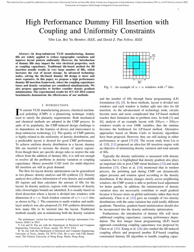
The flow for layout density optimization can be generalizedas two phases: density analysis and fill synthesis [2]. Densityanalysis first collects information of wire density and availablefill regions and then calculates the amount of fills for thelayout. In density analysis, regions with violations of densityrules (lower/upper bound) are identified. It is usually based onfixed dissection where a layout is divided into windows withdimension of w×w. Each window consists of w/r×w/r tilesas shown in Fig. 1. The extension to multi-window and multi-layer analysis was also proposed [3]. Fill synthesis determineshow many fills to be inserted into the layout. Traditionalmethods usually aim at minimizing both the density variation

The preliminary version has been presented at Design Automation Con-ference (DAC) in 2015.

Y. Lin and D. Pan are with the Department of Electrical and ComputerEngineering, University of Texas, Austin, TX 78731 USA.

B. Yu was with the Department of Electrical and Computer Engineering,University of Texas, Austin, TX 78731 USA. He is now with CSE Depart-ment, The Chinese University of Hong Kong, Shatin, Hong Kong.

w

wr

Fig. 1: An example of w × w windows with r2 tiles.

and the number of fills through linear programming (LP)formulation [4], [5]. In these methods, layout is divided intowindows and each window is further split into tiles for fillinsertion. As the advancement of technology node, circuitsbecome more and more complicated that LP-based methodreaches their limitation due to problem sizes. In both [1] and[6], analysis of an example layout with 200µm × 200µmwindows results in over 160K variables, thus the runtimebecomes the bottleneck for LP-based method. Alternativeapproaches based on Monte Carlo or heuristic algorithmshave been proposed. However, they are still lacking in eitherperformance or speed [7]–[9]. The recent study from Liu etal. [10], [11] proposed an ultra-fast fill insertion engine withan objective of minimizing density variation and total amountof fills.

Typically the density uniformity is measured with densityvariation, but it is highlighted that density gradient also playsan important role in post-CMP metal thickness [12] and maskdistortion [13]. Chen et al. [14] mentioned that in modernprocess, the polishing pad during CMP can dynamicallyadjust pressure and rotation speed according to the densitydistribution. If the density changes slowly across neighboringwindows, the CMP system is able to perform local adjustmentfor better quality. In addition, the minimization of densityvariation does not necessarily contribute to small gradientbecause it focuses more on global uniformity rather than localuniformity. Chen et al. [12] gave an example of two densitydistributions with the same variation but yield totally differentgradients. Therefore, gradient based minimization should alsobe incorporated into the density uniformity optimization.

Furthermore, the introduction of dummy fills will incuradditional coupling capacitance, causing performance degra-dation. The first integer linear programming (ILP) basedapproach considering coupling capacitance was proposed byChen et al. [15]. Xiang et al. [16] also studied the fill-inducedcoupling effects and proposed another ILP-based couplingconstrained dummy fill algorithm to handle coupling capac-



itance. Their methods efficiently analyze density distributionand conduct fill optimization based on slots.

Besides runtime, another problem for traditional tile-basedapproaches lies in the requirement of large amount of fills forgood uniformity, resulting in the difficulty for layout storage.Although current layout file standard like GDSII and OASIScan achieve good reduction in data volume, the problem isnot solved due to the increasing complexity of circuits. Inaddition, large file size often leads to usability limitation andalso increases data transfer time [17]. Ellis et al. [18] andChen et el. [19] made early trials for data compression inGDSII and OASIS for tile based fills. They try to utilize thosearray tokens in the file formats to describe those regular fillmatrices so that the data is compressed with a hierarchicalstructure, such as AREF in GDSII. This approach is suitableto tile based fills because those tiles are regularly aligned. Butin our problem, as fills are described as arbitrary rectangles,which is not regular, it is difficult to wrap them in hierarchy.

To motivate the development of more effective dummy fillalgorithms, ICCAD 2014 held a dummy fill contest [17] andreleased a suite of industrial benchmarks. Many conventionalissues and emerging concerns were holistically modeled withlayer overlay, density variation, line hotspots, outlier hotspotsand file size. A dummy fill optimizer with comprehensiveoptimization is desired. The definitions of these conceptswill be discussed in detail in the next section (Section II).Besides metrics based on density variation from ICCAD 2014contest, the density gradient should also be considered forthe reason of better CMP quality and mask distortion asmentioned above. This is a brand new challenge for multi-objective optimization that includes density, coupling, and filesize for arbitrary rectangular shapes of fills.

In this paper, we develop a high-performance frameworkfor dummy fill insertion. Our main contributions can besummarized as follows.

1) The dummy fill insertion is based on geometric prop-erties instead of tiles. Target density planning is doneat window level and then candidate fills are generatedunder the guidance of target density.

2) The proposed algorithm optimizes for multiple ob-jectives including density variation, density gradient,overlay and so on.

3) We propose an ILP formulation and then its dual min-cost flow formulation to optimize overlay and layoutdensity efficiently.

4) Experimental results show that our algorithms outper-form the top teams by over 10% on ICCAD 2014 DFMcontest benchmarks [17].

The rest part of this paper is organized as follows: Section IIshows the definitions of related concepts and problem for-mulation. Section III explains the optimization algorithms indetail. Section IV presents the experimental results in differentscores. In the end, we conclude our work in Section V.

II. PRELIMINARIES

A. Overlay Between LayersThe spatial overlaps between neighboring layers will lead

to coupling capacitance, which is not desired in the layout de-

Layer 1Layer 2Layer 3

(a)

N Columns

MR

ows

(b)

Fig. 2: Example of (a) overlay between layers (b) squarewindows for density analysis.

sign. Dummy fills are actually metal tiles, and their interactionwith other signal wires will inevitably introduce additionalcapacitance, resulting in performance degradation. Therefore,it is necessary to avoid coupling capacitance during dummyfill insertion. In this work (as in ICCAD 2014 contest),coupling capacitance is evaluated with the amounts of overlayarea between fills and their neighboring layers (includingsignal wires and fills) [20], [21]. As shown in Fig. 2(a), theenclosure regions of orange lines are counted to overlay area.

B. Layout Density

The performance of CMP is highly related to the layoutdensity of a given window, and uniform density distributioncontributes to high CMP quality [6]. In other words, densityvariation along windows is very critical, and is also thepurpose of introducing dummy fills.

The distribution of window densities in this work is eval-uated with three scores: variation, line hotspots, and outlierhotspots [20], [21]. The whole layout is divided into N ×Msquare windows as shown in Fig. 2(b). Variation is standarddeviation of window layout densities, represented with σ. Itaims at capturing the uniformity at layout level. Line hotspotsare summation of column-based variation. For a layout shownin Fig. 2(b), we compute line hotspots as follows,

lh =N∑i=1

M∑j=1

|d(i, j)−∑Mj=1 d(i, j)

M|, (1)

where d(i, j) stands for the layout density at window (i, j).This score is used to verify variations along each column.Outlier hotspots are summation of outlier deviations. Thisscore is designed to evaluate the deviation of window densitiesoutside 3σ range,

oh =N∑i=1

M∑j=1

max(0, |d(i, j)− d| − 3σ), (2)

where d denotes the average density over the layout, and σindicates the variation.

All the 3 scores above evaluate different perspectives of thedensity distribution, and all are used in ICCAD 2014 contest.Variation may only provide a general view to the density map,while line hotspots and outlier hotspots collect more concreteinformation about it.

Besides the metrics on density variations, the uniformityshould also include density gradient whose importance has



been addressed in previous work [12], [13]. We define thedensity gradient g(i, j) for a window (i, j) as follows,

g(i, j) = max(|d(i, j)− d(i+ 1, j)|, |d(i, j)− d(i− 1, j)|,|d(i, j)− d(i, j + 1)|, |d(i, j)− d(i, j − 1)|), (3a)

avg. grad. =N∑i=1

M∑j=1

g(i, j), (3b)

max. grad. = max g(i, j), ∀i ∈ [1, N ], j ∈ [1,M ]. (3c)

It describes the maximum density gap between current win-dow and its four neighboring windows. The density gradientmetric for the whole layout is measured by average densitygradient in Eqn. (3b) and max density gradient in Eqn. (3c)across all the windows.

C. Problem Formulation

The addition of dummy fills needs a comprehensive viewof the layout. That means both performance degradation andCMP quality should be taken into consideration. Hence, in thiswork, the optimization will focus on a combined objective oflayout overlay and density uniformity.

In ICCAD 2014 contest, all the metrics on layout overlayand density uniformity are normalized to scores. But densitygradient is not included in the metrics. Therefore, we willshow the values of density gradient separately without nor-malization.

Given an input layout with initial fill regions and wiredensities across each window, we insert dummy fills tomaximize the following score and minimize density gradient,

score = αovsov + ασsσ + αlhslh + αohsoh + αfssfs, (4)

where sov = fov(∑l∈L ov(l)) denotes total overlay score

for all layers in set L; sσ = fσ(∑l∈L σ(l)) stands for total

variation score for all layers; slh = flh(∑l∈L lh(l)) means

total line hotspot score for all layers; soh = foh(∑l∈L σ(l) ·∑

l∈L oh(l)) represents total outlier score for all layers;sfs = ffs(fs) is file size score. Function f shows how thescore is calculated with its corresponding variables and it canbe generalized to

f(x) = max (0, 1− x

β), (5)

where αov , ασ , αlh, αoh, αfs and β are benchmark-relatedparameters in the contest, which are defined in Table II ofSection IV.

We can see that overlay, variation, line hotspots and outlierhotspots in each layer are added up for scores. File size scoresfs is introduced to reduce the difficulty for layout storage. InICCAD 2014 contest, GDSII format is used as a standard I/Oformat. As mentioned above, the metric of density gradientdoes not apply to the normalizing function in Eqn. (5).

III. DUMMY FILL INSERTION ALGORITHMS

The flow of our algorithm is summarized in Fig. 3. Afterreading the input fill regions, we need to perform polygondecomposition and assign fill regions to each window. Afterthe available fill regions for each window are calculated, the

Initial Fill Regions Density Planning

Candidate Fill Generation

Output Fills

Density Planning

Dummy Fill Insertion

Fig. 3: Our dummy fill insertion flow.

TABLE I: Notations used in Fill Insertion Problem

sm, wm, am DRC rule for min. spacing, width and areaaw Window areadg Density gap (normalized to area)dt(l) Target density on layer ldt(i, j) Target density for window (i, j)

ov Overlaywi, hi width and height of a candidate fillL Set of layersF (l) Set of fills on layer lO(l) Set of fill overlays between layer l and l + 1

P (l) Set of fill pairs with spacing rule violationse(i, j) Euclidean distance between fills i and j, ∀(i, j) ∈ P (l)

xli, xhi left and right bound of fill i

yli, yhi lower and upper bound of fill i

density distribution is ready for density planning and targetdensities can be obtained. Then we generate candidate fillsaccording to density demands and overlay cost. After this,another round of density planning is performed due to theinconsistency between candidate fills and initial plans. In theend, dummy fills are inserted with proper sizes to improveoverlay and density variations. Table I gives the definitions ofsymbols used in the following explanation.

A. Polygon Decomposition

It is very important to decompose input rectilinear polygonsinto rectangles, because rectangles are usually easier to pro-cess and final fills should also be rectangles. The quality offinal fills is also related to the performance of polygon decom-position. Our polygon decomposition algorithm is extendedfrom the efficient polygon-to-rectangle conversion algorithmfrom [22]. The procedure can also be explained as a scanningline move from bottom to top and cut rectangles one-by-one.It is different from the edge-based decomposition in [10] sincewe do not need to differentiate the corners for duplicatedpoints. We extend the algorithm with one horizontal scanningline and another vertical scanning line. During each cut, twocandidate rectangles will be generated from the scanning lineswhere the better rectangle is chosen. There are various criteriain choosing the rectangles, such as area and aspect ratio.We find that a suitable criterion is essential to work togetherwith candidate fill generation in Section III-D for fewer fills.Intuitively larger and fewer rectangles in general lead to better



performance in terms of file size. It is also observed that fewerrectangles in this step do not always contribute to fewer fillsdue to density requirement. More details will be discussedempirically in Section IV-B.

B. Target Density Planning

Due to the complexity of objective function and largeamounts of windows in a layout, direct optimization overthe locations and sizes of dummy fills across all windows isvery expensive and thus time consuming. Density planningis rather important, since it can serve as a guidance forcandidate fill region generation (Section III-D) and final fillinsertion (Section III-E) in each window. Good density planis also capable of reducing the problem size, and eventuallycontributes to the reduction of run-time.

With the information of feasible fill regions, it is possible tocalculate the density bound of each window. The lower boundfor the window density is the wire density in that window,while its upper bound is usually related to the area of its fillregions.

During this step, we do not consider overlay penalty, sothe goal of density planning is to maximize the density score,the summation of variation score, the line hotspot score andthe outlier hotspot score. It is a function of the density ofeach window in each layer. Actually this objective considersmultiple windows in multiple layers. To simplify the analysis,we assume that in all the following notations, the informationof layers is implicitly included. For each window, its densityd(i, j) is bounded by existing wire density and available fillregions. Let the lower and upper bound of d(i, j) be l(i, j)and u(i, j) respectively.

Definition 1 (Target Layout Density). A density value for onelayer represented by dt. Its relation with d(i, j) can be shownas follows,

d(i, j) =

l(i, j), if dt < l(i, j),u(i, j), if dt > u(i, j),dt, other.

(6)

The density planning problem is now transformed to findthe best dt for maximum density score. To find the best dt,we can analyze the following two cases.

Case I: If the ranges of d(i, j) for all windows are largeenough, we can get a trivial solution that is optimal by setting

dt = max (l(k, n)),∀k ∈ 1, 2, ..., N, n ∈ 1, 2, ...,M. (7)

It means that the target density dt is equal to the largest wiredensity throughout the layout. In this way, an ideal uniformdistribution is achieved since densities in all windows are thesame.

Case II: Not all windows are able to get to target layoutdensity. For example, the largest wire density may be 0.9,while a window can only achieve a density as high as 0.7.This kind of situation will occur when ∃(i, j) satisfies

u(i, j) < max (l(k, n)), (8)

Then the target density for window (i, j) can only be set tou(i, j) instead of max(l(k, n)). In this case, we simply search

all combinations of target layout densities for all layers withsmall steps and then choose the best one. The search rangefor dt can be limited to values between max(l(k, n)) andmin(u(k, n)). The run-time for this step is still very fast dueto the simplicity of each calculation and limited number oflayers.

C. Density Gradient Adjusting

The target density planning approach in Section III-B aimsat maximizing total density score, but it does not take densitygradient into consideration. In order to keep the planneddensity score and meanwhile optimize density gradient, wechoose to locally adjust gradient for each layer without largeperturbation to the existing results. The problem is formulatedinto a quadratic program as follows,

min∑

1≤i≤N,1≤j≤M

dg(i, j) · dg(i, j) + ε∑

1≤i≤N,1≤j≤M

g(i, j) · g(i, j),

(9a)s.t. dg(i, j) = d(i, j)− dt, (9b)

g(i, j) ≥ d(i, j)− d(i± 1, j), (9c)g(i, j) ≥ d(i± 1, j)− d(i, j), (9d)g(i, j) ≥ d(i, j)− d(i, j ± 1), (9e)g(i, j) ≥ d(i, j ± 1)− d(i, j), (9f)l(i, j) ≤ d(i, j) ≤ u(i, j). (9g)

The objective consists of two parts. The first summationcomputes the quadratic density gap between current windowdensity and target layout density. The second summationcomputes the quadratic gradient for all the windows. Wewant to minimize total density gradient and the amounts ofdeviation from target layout density. Coefficient ε is used tobalance the priority between two parts, and it is set to 10 inthe experiment. The density gap for each window is calculatedin Constraint (9b) where dt denotes the target layout densityobtained from Section III-B. Constraints (9c) to (9f) computethe gradient defined in Eqn. (3a). Since the density gradientfor a window is defined as the maximum density gap betweenthe window and its four neighbors, it introduces four sets ofconstraints for each window. At the same time, it is necessaryto enumerate all the combinations of a−b and b−a to mimicthe absolute operation |a− b| in the density gap computation.So each set contains two constraints. The constraints fromConstraints (9c) to (9f) represent the eight constraints for eachwindow.

Problem (9) is a mathematical program with a quadraticobjective function subject to linear equality and inequalityconstraints; in other words, it is a quadratic program. If werewrite the objective as a general expression, 1

2dTΦd, we

can see that the Hessian matrix Φ is positive semidefinite,which means the quadratic program (9) is a convex quadraticprogramming problem. It can be solved in polynomial time byinterior point method and the constraints can be integrated intothe objective by barrier functions. By solving the quadraticprogram (9), we can obtain locally adjusted density distri-bution with trade-offs between density gradient and density



1

23Layer 1Layer 2

Layer 1 FillLayer 2 Fill

(a) (b)

Fig. 4: Case I Zero Overlay: Example of (a) Fill Regionsin Neighboring Layers in a Window (b) Fill Solution withoutOverlay.

1

2Layer 1Layer 2


3

(a) (b)

Fig. 5: Case II Non-zero Overlay: Example of (a) Fill Regionsin Neighboring Layers in a Window (b) Fill Solution withOverlay.

scores. The solution of d(i, j) for each window will be usedas the target density for each window (i, j).

D. Candidate Fill Region Generation

In this section, we generate candidate fills in each windowunder the guidance of target density and at the same timeminimize overlay. After this step, with all the candidate fills,the density in a window will be no less than its target density.So the output of this step is an upper bound of fills whichneeds further optimization in the next section to reduce densityvariation. For convenience, we only use 2 layers to explainour strategies.

To optimize overlay area, it is necessary to consider fillregions in multiple layers simultaneously. The problem canbe analyzed from two cases.

Case I Zero Overlay: Fig. 4(a) shows one case of fillregions for 2 neighboring layers. We can divide these fillregions into 3 parts, marked as 1, 2 and 3 in the figure. InRegion 1, there is only one empty space in Layer 1 and thesame space in Layer 2 should contain signal wires. If dummyfills are inserted to Layer 1 in this region, it is likely to haveoverlay with wires in Layer 2, since in this region there is wiredistribution with a certain density. In Region 2, the conditionis similar to Region 1 and Layer 1 contains signal wires, whileit is empty in Layer 2. In Region 3, spaces in both layers arefree of signal wires. There is no need to consider overlay withsignal wires any more in this region. But we should be awareof overlay between fills in different layers. If we only insertfills to Region 3, it is possible to achieve zero overlay, asshown in Fig. 4(b).

Case II Non-zero Overlay: Fig. 5(a) shows that Region 3may be too small to meet the density requirements. In thiscase, if we still limit fills inside Region 3, there will beinevitable deterioration in density variation. So the extensionof fills to Region 1 and 2 becomes a necessity and small fill-to-fill overlay is also allowed for better density distribution.

We evaluate the quality of a candidate fill using a scoreconsidering its overlay with fills in lower and upper layersand its area, shown as Eqn. (10),

q = −fill overlayfill area

+ γ · fill area

window area, (10)

where γ is a parameter, and we set it to 1 in the experiment.Fills with high quality scores have priority in candidate fillselection.

Algorithm 1 Candidate Fill Region Generation

Require: Feasible fill regions of all layers in a window.Ensure: Generate candidate fills with small overlay under

density constraints.1: Assume layer numbers in layer set L are 1, 2, . . . , N;2: Define fr(l) as the fill region in Layer l;3: Define dt(l) as the target density in Layer l;4: Define dw(l) as the wire density in Layer l;5: Define dg(l) as the density gap in Layer l;6: Define d(l) as the layout density of Layer l;7: Define aw as the area of the window;8: Define λ as a parameter, λ ≥ 1;9: for l = odd number of layers in L do

10: frs = intersect(fr(l), fr(l + 1));11: dg(l) = dt(l)− dw(l);12: dg(l + 1) = dt(l + 1)− dw(l + 1);13: if area(frs) ≥ (dg(l) + dg(l + 1)) · aw then14: Assign fills to Layer l until d(l) ≥ λ · dt(l);15: else16: Sort fills in fr(l) by area;17: Assign fills to Layer l until d(l) ≥ λ · dt(l);18: end if19: end for20: for l = even number of layers in L do21: dg(l) = dt(l)− dw(l);22: Sort fills in fr(l) by quality score q;23: Assign fills to Layer l until d(l) ≥ λ · dt(l);24: end for

Since the number of layers is usually larger than 2, theactual implementation combines the previous ideas, which issummarized in Alg. 1. It is impossible to calculate the overlaybetween fills before any fill is inserted to the lower/upperlayer, so we determine candidate fills in odd layers first asa reference for even layers. Function intersect returns theshared fill region between fr(l) and fr(l + 1). If the sharedfill region fails to meet the density requirements in layer land layer l + 1, fill qualities are simply evaluated with thesize of the fill. After the generation of candidate fills in oddlayers, we select fills in even layers according to their qualityscore q with Eqn. (10). λ is a parameter to control how manyfills to generate for each layer. It is no less than 1 becausethe amount of fills should be large enough to achieve targetdensity.

Although Alg. 1 considers both density benefit and overlaycost, it cannot handle some special cases, shown as Fig. 6(a).Sometimes there are very few choices for candidate fills in awindow and all the rectangular regions have large overlay with



Window


(a) (b)

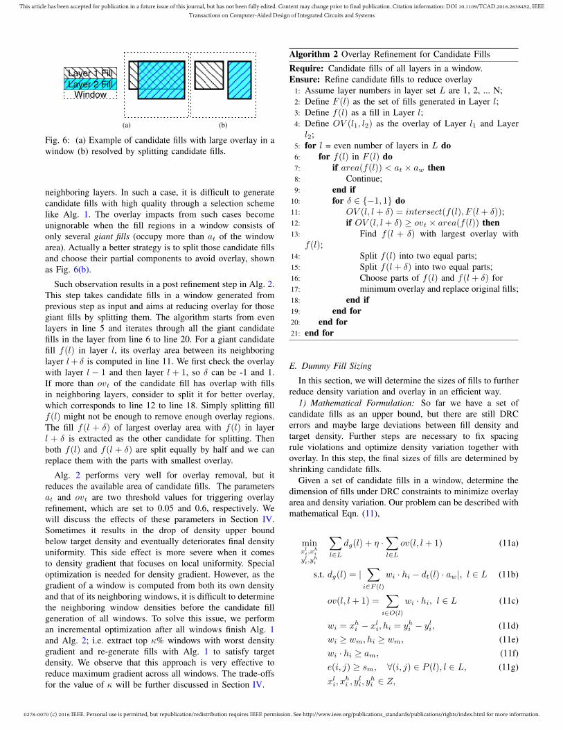
Fig. 6: (a) Example of candidate fills with large overlay in awindow (b) resolved by splitting candidate fills.

neighboring layers. In such a case, it is difficult to generatecandidate fills with high quality through a selection schemelike Alg. 1. The overlay impacts from such cases becomeunignorable when the fill regions in a window consists ofonly several giant fills (occupy more than at of the windowarea). Actually a better strategy is to split those candidate fillsand choose their partial components to avoid overlay, shownas Fig. 6(b).

Such observation results in a post refinement step in Alg. 2.This step takes candidate fills in a window generated fromprevious step as input and aims at reducing overlay for thosegiant fills by splitting them. The algorithm starts from evenlayers in line 5 and iterates through all the giant candidatefills in the layer from line 6 to line 20. For a giant candidatefill f(l) in layer l, its overlay area between its neighboringlayer l+ δ is computed in line 11. We first check the overlaywith layer l − 1 and then layer l + 1, so δ can be -1 and 1.If more than ovt of the candidate fill has overlap with fillsin neighboring layers, consider to split it for better overlay,which corresponds to line 12 to line 18. Simply splitting fillf(l) might not be enough to remove enough overlay regions.The fill f(l + δ) of largest overlay area with f(l) in layerl + δ is extracted as the other candidate for splitting. Thenboth f(l) and f(l + δ) are split equally by half and we canreplace them with the parts with smallest overlay.

Alg. 2 performs very well for overlay removal, but itreduces the available area of candidate fills. The parametersat and ovt are two threshold values for triggering overlayrefinement, which are set to 0.05 and 0.6, respectively. Wewill discuss the effects of these parameters in Section IV.Sometimes it results in the drop of density upper boundbelow target density and eventually deteriorates final densityuniformity. This side effect is more severe when it comesto density gradient that focuses on local uniformity. Specialoptimization is needed for density gradient. However, as thegradient of a window is computed from both its own densityand that of its neighboring windows, it is difficult to determinethe neighboring window densities before the candidate fillgeneration of all windows. To solve this issue, we performan incremental optimization after all windows finish Alg. 1and Alg. 2; i.e. extract top κ% windows with worst densitygradient and re-generate fills with Alg. 1 to satisfy targetdensity. We observe that this approach is very effective toreduce maximum gradient across all windows. The trade-offsfor the value of κ will be further discussed in Section IV.

Algorithm 2 Overlay Refinement for Candidate Fills

Require: Candidate fills of all layers in a window.Ensure: Refine candidate fills to reduce overlay

1: Assume layer numbers in layer set L are 1, 2, ... N;2: Define F (l) as the set of fills generated in Layer l;3: Define f(l) as a fill in Layer l;4: Define OV (l1, l2) as the overlay of Layer l1 and Layerl2;

5: for l = even number of layers in L do6: for f(l) in F (l) do7: if area(f(l)) < at × aw then8: Continue;9: end if

10: for δ ∈ {−1, 1} do11: OV (l, l + δ) = intersect(f(l), F (l + δ));12: if OV (l, l + δ) ≥ ovt × area(f(l)) then13: Find f(l + δ) with largest overlay with

f(l);14: Split f(l) into two equal parts;15: Split f(l + δ) into two equal parts;16: Choose parts of f(l) and f(l + δ) for17: minimum overlay and replace original fills;18: end if19: end for20: end for21: end for

E. Dummy Fill Sizing

In this section, we will determine the sizes of fills to furtherreduce density variation and overlay in an efficient way.

1) Mathematical Formulation: So far we have a set ofcandidate fills as an upper bound, but there are still DRCerrors and maybe large deviations between fill density andtarget density. Further steps are necessary to fix spacingrule violations and optimize density variation together withoverlay. In this step, the final sizes of fills are determined byshrinking candidate fills.

Given a set of candidate fills in a window, determine thedimension of fills under DRC constraints to minimize overlayarea and density variation. Our problem can be described withmathematical Eqn. (11),

minxli,x

hi

yli,yhi

∑l∈L

dg(l) + η ·∑l∈L

ov(l, l + 1) (11a)

s.t. dg(l) = |∑i∈F (l)

wi · hi − dt(l) · aw|, l ∈ L (11b)

ov(l, l + 1) =∑i∈O(l)

wi · hi, l ∈ L (11c)

wi = xhi − xli, hi = yhi − yli, (11d)wi ≥ wm, hi ≥ wm, (11e)wi · hi ≥ am, (11f)e(i, j) ≥ sm, ∀(i, j) ∈ P (l), l ∈ L, (11g)

xli, xhi , y

li, y

hi ∈ Z,



where η is a weight for overlay cost, which is 1 in theexperiment. The objective tries to minimize a combinationof density gap and weighted overlay. In Constraint (11b),density gap dg is defined as the difference between the area offills and the target fill area (derived from target fill density).Constraint (11c) defines the overlay area ov. Constraints (11e)to (11g) state required DRC rules, such as minimum width,minimum area and minimum spacing. e(i, j) is the Euclideandistance between fills i and j. Eqn. (11) defines a non-convexproblem, so it is very expensive to solve it.

2) Problem Relaxation: Previous formulation containsmultiplication operations between variables in two directions,which results in non-convex features. We can alternativelyfix one direction when optimizing the other one, and thenthe problem is relaxed to a linear program. Without lossof generality, we set vertical direction fixed and all thevariables related to that direction become constants. ThenConstraint (11b) and (11c) can be relaxed to

dg(l) = |∑i∈F (l)

wi · hi0 − dt(l) · aw|, l ∈ L, (12)

ov(l, l + 1) =∑i∈O(l)

wi · hi0, l ∈ L, (13)

where hi0 is the initial height of candidate fills from Sec-tion III-D.

Constraints (11e) to (11f) can be merged into one equation,

wi ≥ max(wm,amhi0

). (14)

Constraint (11g) will only exist for pairs of fills that are veryclose to each other. For these fill pairs, following constraintwill force fills to keep enough space in horizontal direction,

eh(i, j) ≥ sm. (15)

With Eqns. (12), (13), (14) and (15), a relaxed problemsolvable with ILP is formed for horizontal direction as fol-lows,

min∑l∈L

dg(l) + η ×∑l∈L

ov(l, l + 1), (16a)

s.t. dg(l) = |∑i∈F (l)

wi × hi0 − dt(l) · aw|, l ∈ L, (16b)

ov(l, l + 1) =∑i∈O(l)

wi × hi0, l ∈ L, (16c)

xhi − xli ≥ max(wm,amhi0

), ∀i ∈ F (l), l ∈ L, (16d)

e(i, j) ≥ sm, ∀(i, j) ∈ P (l), l ∈ L, (16e)

lli ≤ xli ≤ uli, lhi ≤ xhi ≤ uhi , (16f)

xli, xhi ∈ Z,

where dg(l) denotes the density gap in layer l between currentfill area and target fill area as defined in Table I; ov(l, l + 1)denotes the ovelay area between layer l and l + 1; e(i, j)denotes the Euclidean distance between fills i and j thatresult in spacing rule violations. We alternatively optimize theproblem in horizontal and vertical directions. In other words,ILP will be run iteratively. During each iteration, variables

are bounded to a certain range to ensure performance, i.e.lli ≤ xli ≤ uli and lhi ≤ xhi ≤ uhi . These ranges need to beupdated according to the results of each iteration.

3) Dual Min-Cost Flow Formulation: The relaxed problemin previous section may still suffer from high run-time penaltywhen the problem size is large, as ILP problem is generallyNP-hard to solve. Here we show that the formulation is ableto achieve further speedup with dual min-cost flow.

Eqn. (12) contains an absolute operation which ensures thefill density will converge to target density. Since in this stage,fills can only shrink in each iteration. It is possible to relax theproblem by removing the absolute operation. We are alwaysable to calculate the upper bound of fill area by taking thecurrent sizes of fills. If the upper bound is smaller than dt(l) ·aw, then |∑i∈F (l) wi · hi0−dt(l) ·aw| is equivalent to dt(l) ·aw−

∑i∈F (l) wi · hi0. On the other hand, if current fill density

is larger than target density, we can still remove it by reducingthe shrinking steps for fills in each iteration. It should benoted that after current iteration fill density drops below targetdensity, we will switch to the first case and hence the filldensity cannot keep getting away from target density.

Then the relaxed problem in Section III-E2 can be writtenin a generalized manner without any absolute operation,

minxi

N∑i=1

cixi (17a)

s.t. xi − xj ≥ bij , (i, j) ∈ E, (17b)li ≤ xi ≤ ui, i = 1, 2, ..., N, (17c)xi ∈ Z.

Eqn. (17) is a linear program with only differential con-straints and bounded variables, which can be transformed toa dual min-cost flow problem [23]. Min-cost flow problem isa relative mature field with very fast algorithms. Thus it isoften adopted in the physical design flow [24]–[26].

Our problem can be transformed to the following typicaldual min-cost flow format,

minyi

N∑i=0

c′iyi, (18a)

s.t. yi − yj ≥ b′ij , (i, j) ∈ E′, (18b)

yi ∈ Z,

where

xi = yi − y0, i = 1, 2, . . . , N, (19a)

c′i =

{ci, i = 1, 2, . . . , N,

−∑Ni=1 ci, i = 0,

(19b)

b′ij =

bij , (i, j) ∈ E,li, i = 1, 2, . . . , N, j = 0,−ui, i = 0, j = 1, 2, . . . , N.

(19c)

Lemma 1. Eqn. (17) and Eqn. (18) are equivalent.

The proof is omitted here for brevity. The key idea is tointroduce a new variable y0 to convert lower and upper boundconstraints to differential constraints, which is a commontechnique in convex optimization [27].



The corresponding min-cost flow problem can be writtenas follows.

min∑

(i,j)∈E′

−b′ijfij , (20a)

s.t.∑

(j,i)∈E′

fji −∑

(i,k)∈E′

fik = −c′i, i = 0, . . . , N, (20b)

fij ≥ 0, (i, j) ∈ E′. (20c)

So far the dual min-cost flow problem can be mapped to agraph with N + 1 nodes. The supply of node i is c′i and foreach (i, j) pair in E′, an edge starting from node i to node jwith a cost of −b′ij is inserted to the graph. The edge capacityis set to infinity. Final solution of y can be obtained from thepotential of each node and x can be derived from Eqn. (19a).

IV. EXPERIMENTAL RESULTS

Our algorithms were implemented in C++ and tested onan 8-Core 3.40 GHz Linux server with 32 GB RAM. Theresults of ICCAD 2014 contest top three teams are tested ona 2.6 GHz machine with 64 GB RAM. Related results andexecutables are released at link (http://www.cerc.utexas.edu/utda/download/DFI/index.html). LEMON [28] is used as themin-cost flow solver. GUROBI [29] is used as the quadraticprogramming solver. Our solutions have been verified by thecontest organizer [17]. Statistics about benchmarks are listedin Table II. The total amount of input polygons for fill inser-tion is shown as “#P”. The total number of layers is shownas “#L”. It also contains coefficients to calculate followingscores. Since all the metrics are represented in scores, we add“*” to differentiate them from their original values. Overlay∗

denotes the overlay score stated in Section II; Variation∗

represents variation score; Line∗ is the score for line hotspots;Outlier∗ is the score for outlier hotspots; Size∗ is the scorefor the volume of solution GDSII files, which is the standardinput and output format in the contest; Run-time∗ standsfor run-time score; Memory∗ denotes memory score and itmeasures the peak memory usage during the execution. Allthe scores above are calculated with Eqn. (5). According toICCAD 2014 contest [17], Score is the weighted summationof all the scores above. Quality is similar to testcase scorebut excludes run-time score and memory score. It measuresthe quality of solutions. α and β respect to the coefficientsin Eqn. (4) and (5). Run-time score and memory score arealso calculated with Eqn. (5). The fills inserted must liein specific regions given inputs and subject to DRC rules,i.e. minimum metal width and space of 32nm and minimummetal area of 4800nm2. The window size for fill insertionis set to 20x20µm2 according to the contest. All the scoresare obtained from the contest organizer [17] except run-timeand peak memory usage which are measured in the server. Toevaluate the effectiveness of our algorithm, we compare ourresults with top three teams in the contest. In the result tables,our dummy fill insertion algorithm for variation minimizationis shown as “DFI”. Our algorithm with gradient minimizationis shown as “G-DFI”.

Table III lists the evaluation results for our algorithm andtop three teams from the ICCAD 2014 contest. It is shown

that our fill insertion engine produces both the highest qualityscores and overall scores for all the testcases. On average, thequality score of DFI is 13% better and the overall score isabout 10% higher than the top team in the contest. G-DFIfurther improves the quality and efficiency of DFI such thateventually it outperforms the top team by 22% in quality scoreand 24.6% in overall score.

According to score calculation, density related scores (vari-ation, line hotspots and outlier hotspots) take 45%, and over-lay score takes 20%. From Table III we can see that our overalldensity scores are among the highest. e.g. for benchmarkm we get the best density scores, though the overlay scoreis a little bit lower than top three teams. We ascribe it tothe comprehensive density analysis and simultaneous controlover density and overlay during fill insertion. Our densityplanning directly works on the density score metrics includingvariation, line hotspots and outlier hotspots, for optimizingany of metrics individually may not result in a good overallscore. Furthermore, we consider overlay in both candidatefill generation and dummy fill sizing under the guidance ofdensity planning. So the overlay can be reduced withoutdegrading the density scores too much. We can also seethat our size score is high, which means the number of fillsinserted is much smaller than others. Although the contest1st team gets even higher size score, their solutions sufferfrom larger density variation. When the size of layout fileincreases, it takes longer time for reading and writing. Insummary, the results demonstrate that our algorithms producemore balanced solutions which can handle overlay and densityrequirements simultaneously.

We further compare our gradient aware algorithm G-DFIwith DFI together with average and maximum density gradi-ent metrics, shown as Table IV. Grad. Avg/Max is computedthrough the summation of average and maximum gradientvalues across all layers. Since the official evaluation scriptdoes not contain gradient metrics and it is not released either,we try our best to estimate our results as close as possible tothe official values. Comparing the scores in Table III withthat in Table IV and Table V for G-DFI, all the densityrelated metrics are very close. The slight difference comesfrom different starting coordinates of windows which aredetermined by the leftmost lowest shape in the official script.The leftmost lowest shape can be either a dummy fill or aninitial routing segment. As the initial routing is not accessible,we use (0, 0) as the leftmost lowest coordinates as the startingcoordinates of windows. The overlay includes fill-to-fill andfill-to-routing overlaps in the official script. Again, we are notable to access initial routing and what we have is the densitydistribution of routing layers in each window. So we assume auniform distribution of routing segments in each window foroverlay calculation. While it is true that our evaluation scriptproduces different result from the official one, the fidelity andtrends are maintained. So the comparison is fair according tothe same baseline and script.

In Table IV, we can see the maximum gradient of G-DFI is 59.6% better than DFI and the average gradient alsohas 53.6% improvement. The local adjustment for gradientminimization in Section III-C helps to reduce both average

http://www.cerc.utexas.edu/utda/download/DFI/index.html

http://www.cerc.utexas.edu/utda/download/DFI/index.html



TABLE II: ICCAD 2014 Benchmark Statistics

Design #P #L File size Overlay∗ Variation∗ Line∗ Outlier∗ Size∗ Run-time∗ Memory∗

α β α β α β α β α β α β α βs 382K 3 48M 0.2 79154 0.2 0.077 0.2 11.758 0.15 0.014 0.05 32 0.15 60 0.05 1024b 8.1M 3 1.1G 0.2 6111303 0.2 0.517 0.2 3578 0.15 22.801 0.05 2048 0.15 600 0.05 32768m 31.8M 3 2.2G 0.2 10276835 0.2 0.53 0.2 6052 0.15 27.56 0.05 1536 0.15 1200 0.05 32768

TABLE III: Experimental Results on ICCAD 2014 Benchmark for DFI

Design Team Overlay∗ Variation∗ Line∗ Outlier∗ Size∗ Run-time∗ Memory∗ Quality Score

s

1st 0.743 0.636 0.733 1.000 0.976 0.877 0.885 0.621 0.7972nd 0.743 0.909 0.967 0.975 0.103 0.846 0.831 0.675 0.8443rd 0.613 0.985 0.990 1.000 0.158 0.842 0.429 0.676 0.823DFI 0.723 0.948 0.979 0.994 0.887 0.872 0.818 0.724 0.895

G-DFI 0.719 0.977 0.989 1.000 0.938 0.969 0.931 0.734 0.926

b

1st 0.748 0.368 0.364 0.871 0.924 0.515 0.891 0.473 0.5942nd 0.841 0.381 0.534 0.000 0.053 0.513 0.828 0.354 0.4723rd 0.576 0.485 0.601 0.000 0.568 0.554 0.339 0.361 0.461DFI 0.685 0.499 0.470 0.953 0.765 0.351 0.852 0.512 0.607

G-DFI 0.521 0.675 0.670 0.998 0.837 0.886 0.949 0.564 0.745

m

1st 0.598 0.462 0.486 0.204 0.941 0.556 0.845 0.387 0.5132nd 0.668 0.460 0.618 0.000 0.000 0.780 0.761 0.349 0.5043rd 0.510 0.509 0.689 0.000 0.807 0.748 0.772 0.382 0.533DFI 0.493 0.643 0.766 0.088 0.905 0.750 0.786 0.439 0.591

G-DFI 0.425 0.607 0.593 0.967 0.896 0.932 0.917 0.515 0.701

TABLE IV: Comparison of gradient between DFI and G-DFI

Team Grad. Avg/Max

s DFI 0.004/0.023G-DFI 0.001/0.006

b DFI 0.212/1.127G-DFI 0.096/0.539

m DFI 0.141/1.395G-DFI 0.097/0.658

TABLE V: Comparison between G-DFI and [11]

Team Variation∗ Line∗ Outlier∗ Size∗ Quality

s [11] 1.000 1.000 1.000 0.952 0.776G-DFI 0.977 0.987 1.000 0.938 0.768

b [11] 0.528 0.701 0.000 0.778 0.426G-DFI 0.675 0.670 0.998 0.837 0.547

m [11] 0.876 0.939 0.838 0.385 0.548G-DFI 0.607 0.593 0.967 0.896 0.554

and maximum gradients, while the density scores are main-tained. Actually even the density scores turn out to be slightlybetter, we ascribe the reason to the incremental optimizationprocess after Alg. 2 which contributes to the removal of largeoutliers. But this process also results in more overlay becausecandidate fills with large overlay are allowed in those criticalwindows for better gradient. This explains the drop of overlayscore. Eventually the testcase quality scores are improved by8.2%. We also reduce runtime and memory usage by replacingsmart pointers with primitive pointers so that faster access ispossible. The new runtime values for benchmark s, b, and mare 1.8, 68.1, and 81.4 seconds including file IO, respectively.The peak memory usage values are 70.7, 1662.1, and 2732.7

MB, respectively. According to the results in Table III, theabsolute overlay areas for the three benchmarks in G-DFI are0.022, 2.9 and 5.9 mm2, respectively.

For the comparison with [11] in Table V, we can see thatG-DFI outperforms in quality scores about 6.8%. Our qualityscores on benchmark b and m are much better than theirs,while the scores on benchmark s are very close. In benchmarkb and m, our outlier scores are much higher than theirs.We ascribe the improvement to the incremental optimizationmentioned at the end of Section III-D that often helps removeoutliers by regenerating candidate fills for windows with poorgradients.

A. Runtime and Memory Scalability of Algorithm

We also study the scalability of our algorithm in runtimeand memory, as shown in Fig. 7. We create large benchmarksby duplicating benchmark b from 1x to 16x, so the file size ofthe input benchmarks grows from 1.1GB to 17GB. It can beseen that both runtime and memory increase linearly with thesizes of input benchmarks. In the 1x benchmark, the runtimeis less than 100 seconds and peak memory is around 1.7GB,while in the 16x benchmark, the runtime is less than 1100seconds and peak memory is around 25GB. For benchmarkb, the runtime distribution of each step is as follows: polygondecomposition takes around 16% of runtime, two rounds ofdensity planning take 37% of runtime, and dummy fill sizingtakes 34% of runtime.

B. Criteria for Polygon Decomposition

As mentioned in Section III-A, various heuristics canbe applied to polygon decomposition to facilitate candidate



1 3 5 7 9 11 13 15 170

100200300400500600700800900

1,0001,100

Scaling factor of benchmark b

Seco

nds

1 3 5 7 9 11 13 15 170

5

10

15

20

25

30

GB

RuntimeMemory

Fig. 7: Experiment on runtime and memory scalability byscaling benchmark b from 1x to 16x.

fill generation. Since we have both horizontal and verticalscanning lines, the following five criteria are compared.

1) H: always choose the rectangle cut by the horizontalscanning lines.

2) V: always choose the rectangle cut by the verticalscanning lines.

3) LA: always choose the rectangle with larger area duringeach cut.

4) SA: always choose the rectangle with smaller areaduring each cut.

5) AR: always choose the rectangle with an aspect ratiocloser to one during each cut.

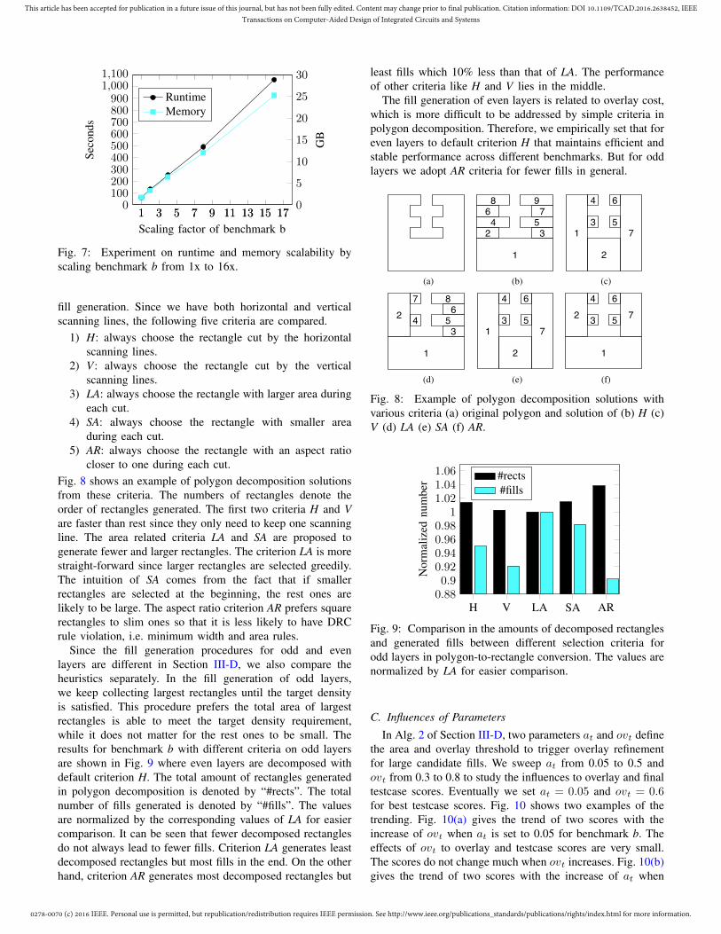
Fig. 8 shows an example of polygon decomposition solutionsfrom these criteria. The numbers of rectangles denote theorder of rectangles generated. The first two criteria H and Vare faster than rest since they only need to keep one scanningline. The area related criteria LA and SA are proposed togenerate fewer and larger rectangles. The criterion LA is morestraight-forward since larger rectangles are selected greedily.The intuition of SA comes from the fact that if smallerrectangles are selected at the beginning, the rest ones arelikely to be large. The aspect ratio criterion AR prefers squarerectangles to slim ones so that it is less likely to have DRCrule violation, i.e. minimum width and area rules.

Since the fill generation procedures for odd and evenlayers are different in Section III-D, we also compare theheuristics separately. In the fill generation of odd layers,we keep collecting largest rectangles until the target densityis satisfied. This procedure prefers the total area of largestrectangles is able to meet the target density requirement,while it does not matter for the rest ones to be small. Theresults for benchmark b with different criteria on odd layersare shown in Fig. 9 where even layers are decomposed withdefault criterion H. The total amount of rectangles generatedin polygon decomposition is denoted by “#rects”. The totalnumber of fills generated is denoted by “#fills”. The valuesare normalized by the corresponding values of LA for easiercomparison. It can be seen that fewer decomposed rectanglesdo not always lead to fewer fills. Criterion LA generates leastdecomposed rectangles but most fills in the end. On the otherhand, criterion AR generates most decomposed rectangles but

least fills which 10% less than that of LA. The performanceof other criteria like H and V lies in the middle.

The fill generation of even layers is related to overlay cost,which is more difficult to be addressed by simple criteria inpolygon decomposition. Therefore, we empirically set that foreven layers to default criterion H that maintains efficient andstable performance across different benchmarks. But for oddlayers we adopt AR criteria for fewer fills in general.

(a)

8642

1

9753

(b)

1 7

2

4

3

6

5

(c)

1

2

7

4

8653

(d)

1 7

2

4

3

6

5

(e)

1

2 7

4

3

6

5

(f)

Fig. 8: Example of polygon decomposition solutions withvarious criteria (a) original polygon and solution of (b) H (c)V (d) LA (e) SA (f) AR.

H V LA SA AR0.880.9

0.920.940.960.98

11.021.041.06

Nor

mal

ized

num

ber #rects

#fills

Fig. 9: Comparison in the amounts of decomposed rectanglesand generated fills between different selection criteria forodd layers in polygon-to-rectangle conversion. The values arenormalized by LA for easier comparison.

C. Influences of Parameters

In Alg. 2 of Section III-D, two parameters at and ovt definethe area and overlay threshold to trigger overlay refinementfor large candidate fills. We sweep at from 0.05 to 0.5 andovt from 0.3 to 0.8 to study the influences to overlay and finaltestcase scores. Eventually we set at = 0.05 and ovt = 0.6for best testcase scores. Fig. 10 shows two examples of thetrending. Fig. 10(a) gives the trend of two scores with theincrease of ovt when at is set to 0.05 for benchmark b. Theeffects of ovt to overlay and testcase scores are very small.The scores do not change much when ovt increases. Fig. 10(b)gives the trend of two scores with the increase of at when



ovt is set to 0.6 for benchmark b. The parameter at has moreimpacts on the overlay score, as it drops with the increaseof at. But the testcase score drops much slower than overlayscore, because performing overlay refinement to more fills ingeneral worsen density scores, such as variation.

As mentioned in Section III-C, the percentage κ in theincremental optimization for candidate fill re-generation isvery critical to both density gradient and variations. Althoughlarger κ contributes to smaller gradient and better densitydistribution, it inevitably leads to more overlays and runtime.Fig. 11 plots the trending of total maximum gradient, totaldensity score and testcase quality score with the growth of κfor benchmark s, b and m. We can see that with the increaseof κ from 2 to 10, total maximum gradient drops quickly andthen saturates afterwards for benchmark b and m. The totaldensity score and overlay score grow in an opposite directionin general from 2 to 20. To trade-off gradient, density andoverlay scores, we use κ = 10 in our implementation.

0.3 0.4 0.5 0.6 0.7 0.80.420.440.460.480.5

0.520.540.56

ovt when at = 0.05

overlay scoretestcase score

(a)

0.1 0.2 0.3 0.4 0.50.420.440.460.480.5

0.520.540.56

at when ovt = 0.6

overlay scoretestcase score

(b)

Fig. 10: Trends of overlay and testcase scores with at andovt. (a) Sweep ovt when at = 0.05. (b) Sweep at whenovt = 0.6.

V. CONCLUSION

This work proposes a new methodology for the holisticfill optimization problem in which file size is included tothe objective along with other cost functions. Experimentalresults show the effectiveness of our algorithms in optimizingmultiple objectives including overlay, density variation, den-sity gradient and file size. In the future work, we will tryto consider exact locations of signal nets to reduce couplingcapacitances rather than only metal density of signal nets fromthe benchmarks. Future work would also include evaluation

0 2 4 6 8 10 12 14 16 18 200.4

0.5

0.6

0.7

0.8

0.9

1

κ

Scor

e

0 2 4 6 8 10 12 14 16 18 200.001

0.003

0.005

0.007

0.009

Gra

dien

t

overlay score total density scoretestcase score total max gradient

(a)

0 2 4 6 8 10 12 14 16 18 200.35

0.4

0.45

0.5

0.55

0.6

0.65

κ

Scor

e

0 2 4 6 8 10 12 14 16 18 200.500

0.550

0.600

0.650

0.700

0.750

Gra

dien

t

(b)

0 2 4 6 8 10 12 14 16 18 200.35

0.4

0.45

0.5

0.55

0.6

0.65

κ

Scor

e

0 2 4 6 8 10 12 14 16 18 200.500

0.550

0.600

0.650

0.700

0.750

Gra

dien

t

(c)

Fig. 11: Trade-offs of percentage κ between gradient, densityand overlays for benchmark (a) s (b) b and (c) m.

on lithography related impacts and methodologies consideringlithograph-friendliness during dummy fill insertion.

ACKNOWLEDGMENT

Thanks to Dr. Rasit Topaloglu for the evaluation of exper-imental results and helpful comments.

APPENDIX

AN EXAMPLE OF DUAL MIN-COST FLOW IN SEC-TION III-E3



Fig. 12(a) gives an example of two candidate fills whereA is in layer 1 and B is in layer 2. Assume in an iterationthe relaxed ILP formulation for horizontal direction can bewritten as follows,

min (x2 − x1) · 8 + (x4 − x3) · 10 + (x2 − x3) · 2, (21a)s.t. x2 − x1 ≥ 8, (21b)

x4 − x3 ≥ 8, (21c)x2 − x3 ≥ 0, (21d)0 ≤ x1 ≤ 4, 6 ≤ x2 ≤ 10,

4 ≤ x3 ≤ 8, 14 ≤ x4 ≤ 18. (21e)

The objective Eqn. (21a) consists of two terms for densityvariations and one term for overlay. Eqn. (21b) to Eqn. (21c)honor DRC rules such as minimum width rules. Eqn. (21d)makes sure the overlay computation in the objective is correct.It is also assumed that initially total area of fills is larger thantarget density, so the absolute operations in the objective canbe removed with tighter bound constraints to each variable.

We can construct the dual min-cost flow graph as Fig. 12(b).Variables x1, x2, x3, x4 correspond to nodes 1, 2, 3, 4,respectively. Each node is labeled with node supply whichcomes from coefficient in the objective Eqn. (21a). For eachdifferential constraint xi−xj ≥ bij , an edge from node i to jis inserted with cost of −bij . For each lower bound constraintxi ≥ li, an edge from node i to t is inserted with cost of −li.For each upper bound constraint xi ≤ ui, an edge from nodes to i is inserted with cost of ui. The capacity for all edges isinfinite. Node s and t corresponds to additional variable y0 forbound constraints added by Eqn. (18). They are regarded asvirtually connected by an undirected edge with zero cost andinfinite capacity. Fig. 12(c) shows the solution graph in whichedges are marked with flow values and nodes are marked withnode potentials. The final solution for xi is the differencebetween the potential of node i and node s/t. So eventuallyx1 = 0, x2 = 8, x3 = 8, x4 = 16.

REFERENCES

[1] A. B. Kahng and K. Samadi, “CMP fill synthesis: A survey of recentstudies,” IEEE Transactions on Computer-Aided Design of IntegratedCircuits and Systems (TCAD), vol. 27, no. 1, pp. 3–19, 2008.

[2] C. Feng, H. Zhou, C. Yan, J. Tao, and X. Zeng, “Efficient approximationalgorithms for chemical mechanical polishing dummy fill,” IEEE Trans-actions on Computer-Aided Design of Integrated Circuits and Systems(TCAD), vol. 30, no. 3, pp. 402–415, 2011.

[3] A. B. Kahng, G. Robins, A. Singh, and A. Zelikovsky, “New multileveland hierarchical algorithms for layout density control,” in IEEE/ACMAsia and South Pacific Design Automation Conference (ASPDAC),1999, pp. 221–224.

[4] ——, “Filling algorithms and analyses for layout density control,” IEEETransactions on Computer-Aided Design of Integrated Circuits andSystems (TCAD), vol. 18, no. 4, pp. 445–462, 1999.

[5] R. Tian, M. D. F. Wong, and R. Boone, “Model-based dummy featureplacement for oxide chemical-mechanical polishing manufacturability,”IEEE Transactions on Computer-Aided Design of Integrated Circuitsand Systems (TCAD), vol. 20, no. 7, pp. 902–910, 2001.

[6] C. Feng, H. Zhou, C. Yan, J. Tao, and X. Zeng, “Provably goodand practically efficient algorithms for CMP,” in ACM/IEEE DesignAutomation Conference (DAC), 2009, pp. 539–544.

[7] Y. Chen, A. B. Kahng, G. Robins, and A. Zelikovsky, “Monte-Carloalgorithms for layout density control,” in IEEE/ACM Asia and SouthPacific Design Automation Conference (ASPDAC), 2000, pp. 523–528.

[8] ——, “Practical iterated fill synthesis for CMP uniformity,” inACM/IEEE Design Automation Conference (DAC), 2000, pp. 671–674.

A

B

x1x1 x2x2 x3x3 x4x4

10

82

(a)

1

2

3

4

ss tt �8,1�8,1 �8,1�8,1 0,10,1

�4,1�4,1

�14,1�14,1

0,10,1

�6,1�6,1

4,14,1

8,18,1

10,110,1

18,118,1

-8 -12

10 10

0,10,1

(b)

-16

-8

-8

0

-16 -168 2 10

0

0

0

0

0

0

0

0

(c)

Fig. 12: (a) Example of fill shrinking problem (b) dual min-cost flow graph (c) corresponding solution graph: edges aremarked with flow values and nodes are marked with potentialvalues.

[9] X. Wang, C. C. Chiang, J. Kawa, and Q. Su, “A min-variance iterativemethod for fast smart dummy feature density assignment in chemical-mechanical polishing,” in IEEE International Symposium on QualityElectronic Design (ISQED), 2005, pp. 258–263.

[10] C. Liu, P. Tu, P. Wu, H. Tang, Y. Jiang, J. Kuang, and E. F. Y. Young,“An effective chemical mechanical polishing filling approach,” in IEEEAnnual Symposium on VLSI (ISVLSI), 2015, pp. 44–49.

[11] C. Liu, P. Tu, P. Wu, H. Tang, Y. Jiang, J. Kuang, and E. F. Young, “Aneffective chemical mechanical polishing fill insertion approach,” ACMTransactions on Design Automation of Electronic Systems (TODAES),vol. 21, no. 3, p. 54, 2016.

[12] H.-Y. Chen, S.-J. Chou, and Y.-W. Chang, “Density gradient minimiza-tion with coupling-constrained dummy fill for CMP control,” in ACMInternational Symposium on Physical Design (ISPD), 2010, pp. 105–111.

[13] P. Wu, H. Zhou, C. Yan, J. Tao, and X. Zeng, “An efficient method forgradient-aware dummy fill synthesis,” Integration, the VLSI Journal,vol. 46, no. 3, pp. 301–309, 2013.

[14] Y. Chen, A. B. Kahng, G. Robins, and A. Zelikovsky, “Closingthe smoothness and uniformity gap in area fill synthesis,” in ACMInternational Symposium on Physical Design (ISPD), 2002, pp. 137–142.

[15] Y. Chen, P. Gupta, and A. B. Kahng, “Performance-impact limited areafill synthesis,” in ACM/IEEE Design Automation Conference (DAC),2003, pp. 22–27.

[16] H. Xiang, L. Deng, R. Puri, K.-Y. Chao, and M. D. F. Wong, “Fastdummy-fill density analysis with coupling constraints,” IEEE Transac-tions on Computer-Aided Design of Integrated Circuits and Systems(TCAD), vol. 27, no. 4, pp. 633–642, 2008.



[17] R. O. Topaloglu, “ICCAD-2014 CAD contest in design for manufac-turability flow for advanced semiconductor nodes and benchmark suite,”in IEEE/ACM International Conference on Computer-Aided Design(ICCAD), 2014, pp. 367–368.

[18] R. B. Ellis, A. B. Kahng, and Y. Zheng, “Compression algorithms fordummy-fill VLSI layout data,” in Proceedings of SPIE, vol. 5042, 2003,pp. 233–245.

[19] Y. Chen, P. Gupta, and A. B. Kahng, “Performance-impact limited-areafill synthesis,” in Proceedings of SPIE, vol. 5042, 2003, pp. 75–86.

[20] R. O. Topaloglu, “Energy-minimization model for fill synthesis,” inIEEE International Symposium on Quality Electronic Design (ISQED),2007, pp. 444–451.

[21] A. B. Kahng and R. O. Topaloglu, “A DOE set for normalization-based extraction of fill impact on capacitances,” in IEEE InternationalSymposium on Quality Electronic Design (ISQED), 2007, pp. 467–474.

[22] K. D. Gourley and D. M. Green, “Polygon-to-rectangle conversionalgorithm,” IEEE Computer Graphics and Applications, vol. 3, no. 1,pp. 31–32, 1983.

[23] R. K. Ahuja, T. L. Magnanti, and J. B. Orlin, Network Flows: Theory,Algorithms, and Applications. Prentice Hall/Pearson, 2005.

[24] J. Vygen, “Algorithms for detailed placement of standard cells,”in IEEE/ACM Proceedings Design, Automation and Test in Eurpoe(DATE), 1998, pp. 321–324.

[25] X. Tang, R. Tian, and M. D. F. Wong, “Optimal redistribution of whitespace for wire length minimization,” in IEEE/ACM Asia and SouthPacific Design Automation Conference (ASPDAC), 2005, pp. 412–417.

[26] S. Ghiasi, E. Bozorgzadeh, P.-K. Huang, R. Jafari, and M. Sarrafzadeh,“A unified theory of timing budget management,” IEEE Transactionson Computer-Aided Design of Integrated Circuits and Systems (TCAD),vol. 25, no. 11, pp. 2364–2375, 2006.

[27] S. Boyd and L. Vandenberghe, Convex Optimization. Cambridgeuniversity press, 2004.

[28] “LEMON,” http://lemon.cs.elte.hu/trac/lemon.[29] Gurobi Optimization Inc., “Gurobi optimizer reference manual,” http:

//www.gurobi.com, 2014.

Yibo Lin received the B.S. degree in microelectron-ics from Shanghai Jiaotong University, Shanghai,China, in 2013. He is currently pursuing the Ph.D.degree in the Department of Electrical and Com-puter Engineering, University of Texas at Austin.His research interests include physical design anddesign for manufacturability.

He has received Best Paper Awards at SPIEAdvanced Lithography Conference 2016.

Bei Yu (S’11–M’14) received his Ph.D. degreefrom the Department of Electrical and ComputerEngineering, University of Texas at Austin in 2014.He is currently an Assistant Professor in the Depart-ment of Computer Science and Engineering, TheChinese University of Hong Kong. He has servedin the editorial boards of Integration, the VLSIJournal and IET Cyber-Physical Systems: Theory& Applications.

He has received three Best Paper Awards at SPIEAdvanced Lithography Conference 2016, Interna-

tional Conference on Computer Aided Design (ICCAD) 2013, and Asia andSouth Pacific Design Automation Conference (ASPDAC) 2012, three otherBest Paper Award Nominations at Design Automation Conference (DAC)2014, ASPDAC 2013, ICCAD 2011, and three ICCAD contest awards in2015, 2013 and 2012.

David Z. Pan (S’97–M’00–SM’06-F’14) receivedhis B.S. degree from Peking University, and hisM.S. and Ph.D. degrees from University of Cali-fornia, Los Angeles (UCLA). From 2000 to 2003,he was a Research Staff Member with IBM T.J. Watson Research Center. He is currently theEngineering Foundation Endowed Professor at theDepartment of Electrical and Computer Engineer-ing, The University of Texas at Austin. He haspublished over 200 papers in refereed journals andconferences, and is the holder of 8 U.S. patents. His

research interests include cross-layer nanometer IC design for manufactura-bility/reliability, new frontiers of physical design, and CAD for emergingtechnologies such as 3D-IC, bio, and nanophotonics.

He has served as a Senior Associate Editor for ACM Transactions onDesign Automation of Electronic Systems (TODAES), an Associate Editorfor IEEE Transactions on Computer Aided Design of Integrated Circuitsand Systems (TCAD), IEEE Transactions on Very Large Scale IntegrationSystems (TVLSI), IEEE Transactions on Circuits and Systems PART I(TCAS-I), IEEE Transactions on Circuits and Systems PART II (TCAS-II),Science China Information Sciences (SCIS), Journal of Computer Science andTechnology (JCST), etc. He has served as Program/General Chair of ISPD,TPC Subcommittee Chair for DAC, ICCAD, ASPDAC, ISLPED, ICCD,Tutorial Chair for DAC 2014, Workshop Chair for ICCAD 2015, amongothers.

He has received a number of awards, including the SRC 2013 TechnicalExcellence Award, DAC Top 10 Author in Fifth Decade, DAC Prolific AuthorAward, ASPDAC Frequently Cited Author Award, 11 Best Paper Awardsand several international CAD contest awards, Communications of the ACMResearch Highlights (2014), ACM/SIGDA Outstanding New Faculty Award(2005), NSF CAREER Award (2007), SRC Inventor Recognition Award threetimes, IBM Faculty Award four times, UCLA Engineering DistinguishedYoung Alumnus Award (2009), and UT Austin RAISE Faculty ExcellenceAward (2014).

http://lemon.cs.elte.hu/trac/lemon

http://www.gurobi.com

http://www.gurobi.com

high performance dummy fill insertion with coupling and ... · layer overlay, density variation,...

Documents