high performance flat plate solar thermal collector evaluation · c. study design and objectives...
TRANSCRIPT

Prepared for the General Services Administration By the National Renewable Energy Laboratory
APRIL 2016
High Performance Flat Plate Solar Thermal Collector Evaluation
CALEB ROCKENBAUGH (NREL)
JESSE DEAN (NREL)
DAVID LOVULLO (NREL)
LARS LISELL (NREL)
GREG BARKER (MEP)
ED HANCKOCK (MEP)
PAUL NORTON (MEP)

The Green Proving Ground program leverages GSA’s real estate portfolio to evaluate innovative sustainable building technologies and practices. Findings are used to support the development of GSA performance specifications and inform decision-making within GSA, other federal agencies, and the real estate industry. The program aims to drive innovation in environmental performance in federal buildings and help lead market transformation through deployment of new technologies.
HIGH PE RFORMANCE FLAT PLATE SOLAR THE RMAL COLLE CTOR E VALUATION 1
Disclaimer This document was prepared as an account of work sponsored by the United States Government. While this document is believed to contain correct information, neither the United States Government nor any agency thereof, nor the National Renewable Energy Laboratory, nor any of their employees, makes any warranty, express or implied, or assumes any legal responsibility for the accuracy, completeness, or usefulness of any information, apparatus, product, or process disclosed, or represents that its use would not infringe privately owned rights. Reference herein to any specific commercial product, process, or service by its trade name, trademark, manufacturer, or otherwise, does not constitute or imply its endorsement, recommendation, or favoring by the United States Government or any agency thereof, or the National Renewable Energy Laboratory. The views and opinions of authors expressed herein do not necessarily state or reflect those of the United States Government or any agency thereof or the National Renewable Energy Laboratory.
The work described in this report was funded by the U.S. General Services Administration [and the Federal Energy Management Program of the U.S. Department of Energy] under Interagency Agreement Number (IAG) 14-1947.
Acknowledgements United States General Services Administration (GSA) Green Proving Ground: Kevin Powell, Mike Lowell, Michael Hobson
Major General Emmett J. Bean Center: Alan Miller, Ryan J. Raschke
GSA Regional Headquarters Building Auburn, WA: Marty Novini
TIGI: Zvika Kiler, Ori Spigelman, Doron Yassur
National Renewable Energy Laboratory: Andy Walker, Alicen Kandt, Dylan Cutler
For more information contact:
Kevin Powell Program Manager, GSA Green Proving Ground Office of the Commissioner, Public Buildings Service U.S. General Services Administration 50 United Nations Plaza San Francisco, CA 94102 Email: [email protected]

HIGH PE RFORMANCE FLAT PLATE SOLAR THE RMAL COLLE CTOR E VALUATION 2
List of Acronyms BAS building automation system Btu British thermal unit DHW domestic hot water EIA Energy Information Administration EISA Energy Independence and Security Act of 2007 GSA General Services Administration HSTC Honeycomb Solar Thermal Collector NREL National Renewable Energy Laboratory O&M operations and maintenance OPD overheat protection device PV solar photovoltaic SHW solar thermal water SPF Solartechnik Prufung Forschung SRCC U.S. Solar Rating and Certification Corporation TI transparent insulation
HIGH PE RFORMANCE FLAT PLATE SOLAR THE RMAL COLLE CTOR E VALUATION 3
Table of Contents I. EXECUTIVE SUMMARY 5
A. Background................................................................................................................................ 5
B. Overview of the Technology ..................................................................................................... 5
C. STUDY DESIGN AND OBJECTIVES............................................................................................... 5
D. Project Results/Findings ............................................................................................................ 6
E. Deployment Recommendations.............................................................................................. 10
II. INTRODUCTION 12
A. Problem Statement ................................................................................................................. 12
B. Opportunity ............................................................................................................................. 12
C. Technology Description ........................................................................................................... 13
III. METHODOLOGY 17
A. Technical Objectives ................................................................................................................ 17
B. Criteria for Site selection ......................................................................................................... 19
IV. MEASUREMENT & VERIFICATION EVALUATION PLAN 20
A. Facility Description .................................................................................................................. 20
B. Technology Deployment ......................................................................................................... 21
C. Measurement and Verification ............................................................................................... 24
AUBURN SITE ................................................................................................................................. 27
V. RESULTS 30
VI. SUMMARY FINDINGS AND CONCLUSIONS 59
A. Overall Technology Assessment at Demonstration Facility .................................................... 59
B. Best Practice ............................................................................................................................ 60
C. Recommendations for Installation, Commissioning, Training, and Change Management ..... 61
VII. APPENDICES 63
Appendix A – Parameters Used in Simulations .............................................................................. 63
Appendix B – Delivered Energy Cost vs. Collector Area, HSTC ...................................................... 67
Appendix C – Delivered Energy Cost vs. Collector Area, Typical Flat-Plate Collector .................... 68
Appendix D – Delivered Energy Cost vs. Area/Load Ratio, HSTC ................................................... 69
Appendix E – Delivered Energy Cost vs. Area/Load Rati, Typical Flat-Plate Collector .................. 70
Appendix F – Delivered Energy Cost vs. Solar Fraction, HSTC ....................................................... 71

HIGH PE RFORMANCE FLAT PLATE SOLAR THE RMAL COLLE CTOR E VALUATION 4
Appendix G – Delivered Energy Cost vs. Solar Fraction, Typical Flat-Plate Collector .................... 72
Appendix H – Comparisons of Delivered Energy Costs, HSTC vs. Standard Flat-Plate .................. 73
Appendix I – Nomenclature ........................................................................................................... 75
Appendix J – Glossary .................................................................................................................... 77
Appendix K – References ............................................................................................................... 78
HIGH PE RFORMANCE FLAT PLATE SOLAR THE RMAL COLLE CTOR E VALUATION 5
I. Executive Summary
A. Background Solar thermal water heating or solar hot water (SHW) has a long history of use throughout the world, but has had varying penetration in the U.S. market due to a combination of relatively high system cost and low cost of fuels being offset. Solar energy technologies offer a number of strategic benefits to the United States as sunlight is a free resource; once solar technologies are installed, they have very low operating costs and require minimal non-solar inputs. According to the Energy Information Administration (EIA), domestic hot water (DHW) accounted for 6.7% of commercial building energy use, and solar energy supplied approximately 2% of the 6.7% (0.05 Quads/year) in 2010 [1]. EIA also estimated that 3% of commercial buildings have solar thermal systems; for those facilities, approximately one third of the DHW load is supplied by the on-site solar thermal system.
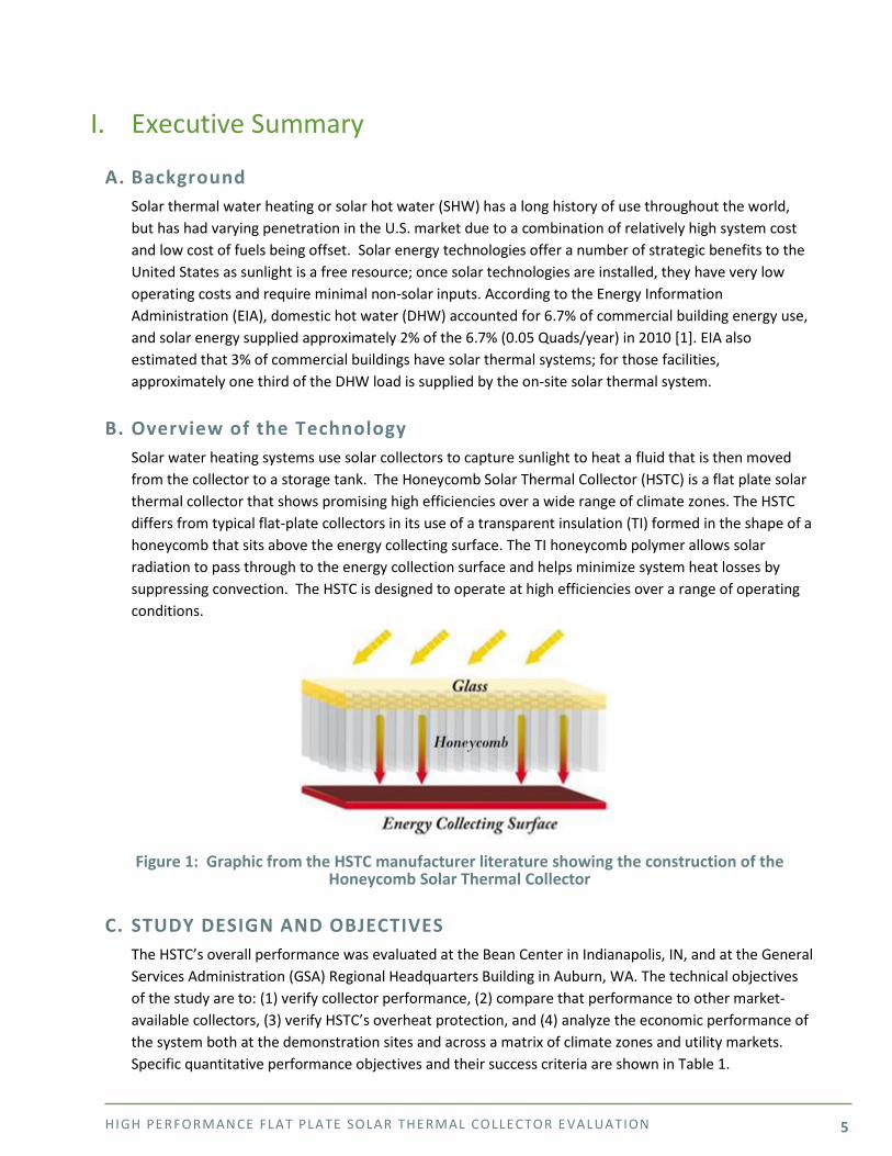
B. Overview of the Technology Solar water heating systems use solar collectors to capture sunlight to heat a fluid that is then moved from the collector to a storage tank. The Honeycomb Solar Thermal Collector (HSTC) is a flat plate solar thermal collector that shows promising high efficiencies over a wide range of climate zones. The HSTC differs from typical flat-plate collectors in its use of a transparent insulation (TI) formed in the shape of a honeycomb that sits above the energy collecting surface. The TI honeycomb polymer allows solar radiation to pass through to the energy collection surface and helps minimize system heat losses by suppressing convection. The HSTC is designed to operate at high efficiencies over a range of operating conditions.
Figure 1: Graphic from the HSTC manufacturer literature showing the construction of the
Honeycomb Solar Thermal Collector
C. STUDY DESIGN AND OBJECTIVES The HSTC’s overall performance was evaluated at the Bean Center in Indianapolis, IN, and at the General Services Administration (GSA) Regional Headquarters Building in Auburn, WA. The technical objectives of the study are to: (1) verify collector performance, (2) compare that performance to other market-available collectors, (3) verify HSTC’s overheat protection, and (4) analyze the economic performance of the system both at the demonstration sites and across a matrix of climate zones and utility markets. Specific quantitative performance objectives and their success criteria are shown in Table 1.
HIGH PE RFORMANCE FLAT PLATE SOLAR THE RMAL COLLE CTOR E VALUATION 6
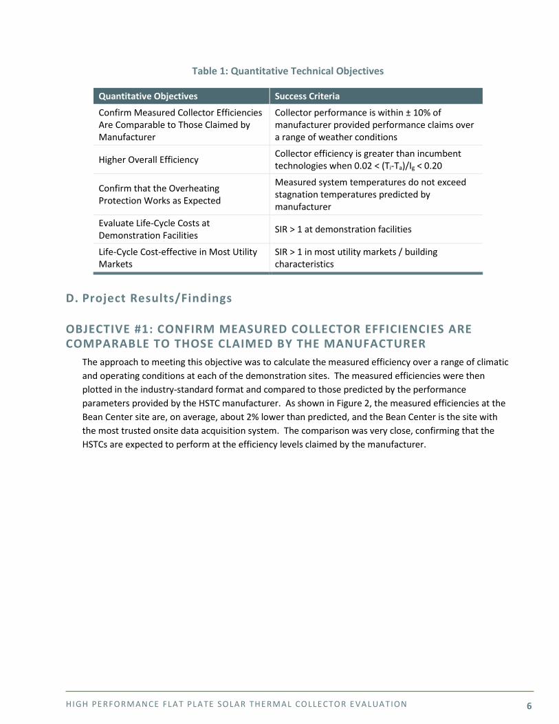
Table 1: Quantitative Technical Objectives
Quantitative Objectives Success Criteria
Confirm Measured Collector Efficiencies Are Comparable to Those Claimed by Manufacturer
Collector performance is within ± 10% of manufacturer provided performance claims over a range of weather conditions
Higher Overall Efficiency Collector efficiency is greater than incumbent technologies when 0.02 < (Ti-Ta)/Ig < 0.20
Confirm that the Overheating Protection Works as Expected
Measured system temperatures do not exceed stagnation temperatures predicted by manufacturer
Evaluate Life-Cycle Costs at Demonstration Facilities SIR > 1 at demonstration facilities
Life-Cycle Cost-effective in Most Utility Markets
SIR > 1 in most utility markets / building characteristics
D. Project Results/Findings
OBJECTIVE #1: CONFIRM MEASURED COLLECTOR EFFICIENCIES ARE COMPARABLE TO THOSE CLAIMED BY THE MANUFACTURER
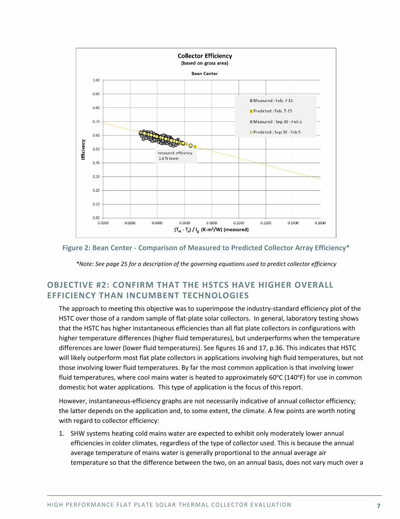
The approach to meeting this objective was to calculate the measured efficiency over a range of climatic and operating conditions at each of the demonstration sites. The measured efficiencies were then plotted in the industry-standard format and compared to those predicted by the performance parameters provided by the HSTC manufacturer. As shown in Figure 2, the measured efficiencies at the Bean Center site are, on average, about 2% lower than predicted, and the Bean Center is the site with the most trusted onsite data acquisition system. The comparison was very close, confirming that the HSTCs are expected to perform at the efficiency levels claimed by the manufacturer.
HIGH PE RFORMANCE FLAT PLATE SOLAR THE RMAL COLLE CTOR E VALUATION 7
Figure 2: Bean Center - Comparison of Measured to Predicted Collector Array Efficiency*
*Note: See page 25 for a description of the governing equations used to predict collector efficiency
OBJECTIVE #2: CONFIRM THAT THE HSTCS HAVE HIGHER OVERALL EFFICIENCY THAN INCUMBENT TECHNOLOGIES
The approach to meeting this objective was to superimpose the industry-standard efficiency plot of the HSTC over those of a random sample of flat-plate solar collectors. In general, laboratory testing shows that the HSTC has higher instantaneous efficiencies than all flat plate collectors in configurations with higher temperature differences (higher fluid temperatures), but underperforms when the temperature differences are lower (lower fluid temperatures). See figures 16 and 17, p.36. This indicates that HSTC will likely outperform most flat plate collectors in applications involving high fluid temperatures, but not those involving lower fluid temperatures. By far the most common application is that involving lower fluid temperatures, where cool mains water is heated to approximately 60oC (140oF) for use in common domestic hot water applications. This type of application is the focus of this report.
However, instantaneous-efficiency graphs are not necessarily indicative of annual collector efficiency; the latter depends on the application and, to some extent, the climate. A few points are worth noting with regard to collector efficiency:
1. SHW systems heating cold mains water are expected to exhibit only moderately lower annual efficiencies in colder climates, regardless of the type of collector used. This is because the annual average temperature of mains water is generally proportional to the annual average air temperature so that the difference between the two, on an annual basis, does not vary much over a
HIGH PE RFORMANCE FLAT PLATE SOLAR THE RMAL COLLE CTOR E VALUATION 8
wide range of climates. The temperature difference is what most strongly influences the efficiency. This has been demonstrated by Christensen and Barker [10].
2. Collector efficiency is not the only metric involved when considering whether a system is cost-effective because a less-efficient collector may cost less, offsetting the loss in energy savings.
3. Collectors such as the HSTC, which exhibit higher efficiencies when the difference between inlet fluid temperature and ambient temperature is high will likely out-perform more conventional collector technologies in applications that run hotter fluid through the collectors. An example of this type of application is one in which the collector array is fed by a hot hydronic loop in a building. In this case the fluid entering the collector is usually close to the hot water set point of 60oC at all times, whereas in the type of application that was simulated for this study the inlet fluid temperature is on average much lower than the set point.
4. Many evacuated-tube collectors appear to have much lower efficiencies than flat-plate collectors because the tubes have space between them, which makes the efficiency based on gross area appear low, but are not indicative of overall system performance.
OBJECTIVE #3: CONFIRM THAT THE OVERHEATING PROTECTION OF HSTC WORKS AS EXPECTED
The approach to meeting this objective was to measure the stagnation temperature of the collectors installed at the Bean Center under full sun. The overheating protection device worked as predicted by the HSTC manufacturer, with a maximum stagnation temperature of 152oC (306oF).
Stagnation is controlled in typical flat-plate collector systems by the appropriate pressurization of the working fluid; a fluid at higher pressure has a higher resulting boiling temperature. Due to the low thermal losses of the HSTC, an overheat protection device is necessary, as excessive pressures may be required to ensure the system does not stagnate.
There has been growing evidence that, even for less-efficient collectors, propylene glycol can be damaged if raised to stagnation temperatures for extended periods of time. The HSTC manufacturer’s approach makes sure that the fluid never reaches these damaging temperatures, which may decrease the maintenance costs of the system over its lifetime, as addressed below.
OBJECTIVE #4: LIFE-CYCLE COST-EFFECTIVE AT DEMONSTRATION FACILITIES
Using an hourly simulation tool and the measured hot water load profile, it was demonstrated that neither of the systems being monitored are expected to be life-cycle cost-effective. The installed costs at each site were much higher than average, leading to a very high life-cycle cost. The hourly simulation tool TRNSYS [2] was utilized to estimate performance for a full 12-month period, covering gaps in data collection. Sensitivities were run on installed system cost to evaluate whether typical installed costs would result in life-cycle cost-effective installations. The lower capital costs still did not result in a system that was cost-competitive in light of the low utility rates at the sites.
HIGH PE RFORMANCE FLAT PLATE SOLAR THE RMAL COLLE CTOR E VALUATION 9
OBJECTIVE #5: COMPARE LIFE-CYCLE COST-EFFECTIVENESS OF HSTC TO STANDARD FLAT PLATE OVER A RANGE OF CLIMATES
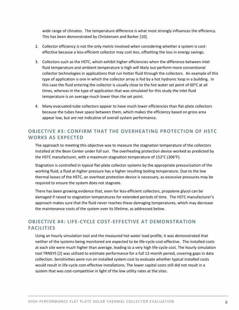
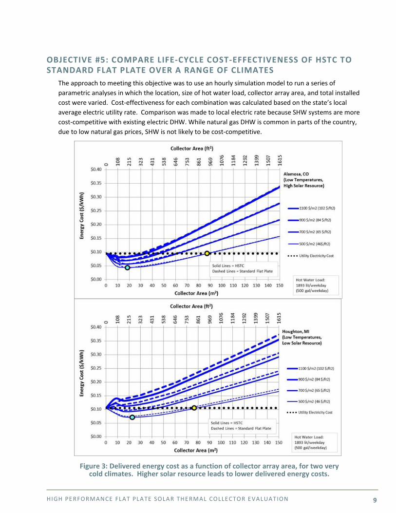
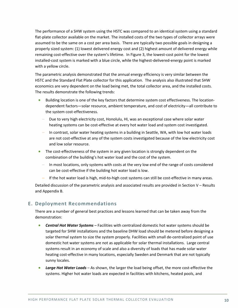
The approach to meeting this objective was to use an hourly simulation model to run a series of parametric analyses in which the location, size of hot water load, collector array area, and total installed cost were varied. Cost-effectiveness for each combination was calculated based on the state’s local average electric utility rate. Comparison was made to local electric rate because SHW systems are more cost-competitive with existing electric DHW. While natural gas DHW is common in parts of the country, due to low natural gas prices, SHW is not likely to be cost-competitive.
Figure 3: Delivered energy cost as a function of collector array area, for two very cold climates. Higher solar resource leads to lower delivered energy costs.
HIGH PE RFORMANCE FLAT PLATE SOLAR THE RMAL COLLE CTOR E VALUATION 10
The performance of a SHW system using the HSTC was compared to an identical system using a standard flat-plate collector available on the market. The installed costs of the two types of collector arrays were assumed to be the same on a cost per area basis. There are typically two possible goals in designing a properly sized system: (1) lowest delivered energy cost and (2) highest amount of delivered energy while remaining cost-effective over the system’s lifetime. In Figure 3, the lowest-cost point for the lowest installed-cost system is marked with a blue circle, while the highest-delivered-energy point is marked with a yellow circle.
The parametric analysis demonstrated that the annual energy efficiency is very similar between the HSTC and the Standard Flat Plate collector for this application. The analysis also illustrated that SHW economics are very dependent on the load being met, the total collector area, and the installed costs. The results demonstrate the following trends:
• Building location is one of the key factors that determine system cost effectiveness. The location-dependent factors—solar resource, ambient temperature, and cost of electricity—all contribute to the system cost-effectiveness.
− Due to very high electricity cost, Honolulu, HI, was an exceptional case where solar water heating systems can be cost-effective at every hot water load and system cost investigated.
− In contrast, solar water heating systems in a building in Seattle, WA, with low hot water loads are not cost-effective at any of the system costs investigated because of the low electricity cost and low solar resource.
• The cost-effectiveness of the system in any given location is strongly dependent on the combination of the building’s hot water load and the cost of the system.
− In most locations, only systems with costs at the very low end of the range of costs considered can be cost-effective if the building hot water load is low.
− If the hot water load is high, mid-to-high cost systems can still be cost-effective in many areas.
Detailed discussion of the parametric analysis and associated results are provided in Section V – Results and Appendix B.
E. Deployment Recommendations There are a number of general best practices and lessons learned that can be taken away from the demonstration:
• Central Hot Water Systems – Facilities with centralized domestic hot water systems should be targeted for SHW installations and the baseline DHW load should be metered before designing a solar thermal system to size the system properly. Facilities with small de-centralized point of use domestic hot water systems are not as applicable for solar thermal installations. Large central systems result in an economy of scale and also a diversity of loads that has made solar water heating cost-effective in many locations, especially Sweden and Denmark that are not typically sunny locales.
• Large Hot Water Loads – As shown, the larger the load being offset, the more cost-effective the systems. Higher hot water loads are expected in facilities with kitchens, heated pools, and
HIGH PE RFORMANCE FLAT PLATE SOLAR THE RMAL COLLE CTOR E VALUATION 11
showers. GSA facilities with these larger loads should be targeted. It is important that water loads are consistent throughout the week and throughout the year.
• High Energy Costs – The natural gas industry has experienced significant cost reductions over the last few years. The economics of the solar thermal system is sensitive to fuel source costs; the unit cost of energy from electricity is many times higher than natural gas in certain locations. Locations with electric resistance domestic hot water heaters and high electric rates should be targeted. Solar water heating also competes with the high costs of propane and fuel oil.
• Use Accurate System Design Tools to Calculate Life-Cycle Costs and Optimize Cost Effectiveness – An approach to determining the correct system design to meet a particular cost-effectiveness objective has been demonstrated in this report. It is recommended that this approach be followed when evaluating whether or not to install an SHW system at a particular facility. A detailed sub-hourly simulation program should be used and the system should be modeled accurately with SRCC-rated solar thermal panel performance data. This will aid in the correct sizing of the system and enable a more accurate economic analysis.
• Collector Efficiency – The demonstration showed that HSTCs are some of the most efficient collectors on the market for higher-fluid-temperature applications such as industrial process heat, space heating, and hot water hydronic loop re-heating, but show only moderate performance improvement, for some climates, for standard domestic hot water applications where ground-temperature water is heated to a setpoint. However, collector efficiency is only one part of a large number of factors that influence the overall life-cycle cost of the SHW system. In some instances, a less-efficient but less-expensive collector may be preferable. When the cost effectiveness of the SHW system is the ultimate metric upon which decisions are to be made, the choice of which collector to use should be based on the procedure outlined in this report, which takes into account the performance and costs of all parts of the SHW system.
• Trained System Installers – It is important that the designers and installers of a solar hot water system have sufficient training and experience with solar hot water systems. Although in principle the components of a SHW system are similar to other common plumbing components, there are several unique features of SHW systems with which experienced plumbers may not be familiar, such as calculating the required pressure of collector fluid to avoid boiling under stagnation conditions.
• Life-Cycle Costs – The cost-effectiveness of the system in any given location is strongly dependent on the combination of the building’s hot water load and the installed cost of the system.
− In most locations, only systems with costs at the very low end of the range can be cost-effective if the building hot water load is low.
− If the hot water load is high, mid-to-high cost systems can still be cost-effective in many areas, depending on the cost of providing electricity.
• Consider efficiency first – The existing DHW equipment should be analyzed prior to the installation of a SHW system. All applicable water conservation and energy efficiency opportunities should be implemented before sizing a solar thermal system.
HIGH PE RFORMANCE FLAT PLATE SOLAR THE RMAL COLLE CTOR E VALUATION 12
II. Introduction
A. Problem Statement Solar energy technologies offer a number of strategic benefits to the United States as sunlight is a free resource; once solar technologies are installed, they have very low operating costs and require minimal non-solar inputs. This provides increased resilience with respect to conventional fuel supply disruptions and price volatility. In addition, growing the domestic solar energy industry could establish the U.S. as a global leader in solar technology innovation and support a growing number of solar-related jobs.
According to the EIA, DHW accounted for 6.7% of commercial building energy use, and solar energy supplied approximately 2% of the 6.7% (0.05 Quads/year) in 20101. EIA also estimated that 3% of commercial buildings have solar thermal systems; for those facilities, approximately one third of the DHW load is supplied by the on-site solar thermal system. Opportunities to optimize energy efficiency and implement renewable energy technologies for this end use can have a significant impact on reducing the energy use across the GSA portfolio.
Solar thermal water heating or SHW has a long history of use throughout the world, but has had varying penetration in the U.S. market due to a combination of relatively high system cost and low cost of fuels being offset. Various configurations of SHW systems provide the benefit of utilizing solar energy to heat water by circulating a fluid—either water directly or a glycol mixture in conjunction with a heat exchanger—through an absorber that transfers the heat for use in the facility.
One of the primary factors impacting the thermal performance of SHW collectors is the rate of heat loss. Minimizing the heat loss from SHW collectors increases their overall efficiency. By reducing collector heat loss, more of the incident solar energy can be collected and utilized to offset conventional energy use in a facility.
The HSTC is a technology that has been developed to provide greater efficiencies by reducing these losses and incorporating overheat protection which minimizes the stagnation temperature of the fluid in the collector.
B. Opportunity U.S. General Services Administration is responsible for over 354 million ft2 of federally owned and leased space in more than 9,600 buildings [1]. A large percentage of those facilities are candidates for rooftop solar installations.
Targeting energy consumption in federal buildings, the Energy Independence and Security Act of 2007 (EISA) requires new federal buildings and major renovations to meet 30% of their hot water demand with solar energy, provided it is cost-effective over the life of the system.
Currently, DHW systems are primarily served by electric and natural gas heating systems, with natural gas making the largest contribution. Facilities that currently use electric hot water heating are more
1 EIA Solar Thermal Collector Manufacturing Activities 2009, available at: http://www.energybc.ca/cache/solarthermal/www.eia.gov/renewable/annual/solar_thermal/solar.html
HIGH PE RFORMANCE FLAT PLATE SOLAR THE RMAL COLLE CTOR E VALUATION 13
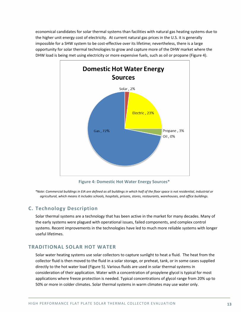
economical candidates for solar thermal systems than facilities with natural gas heating systems due to the higher unit energy cost of electricity. At current natural gas prices in the U.S. it is generally impossible for a SHW system to be cost-effective over its lifetime; nevertheless, there is a large opportunity for solar thermal technologies to grow and capture more of the DHW market where the DHW load is being met using electricity or more expensive fuels, such as oil or propane (Figure 4).
Figure 4: Domestic Hot Water Energy Sources*
*Note: Commercial buildings in EIA are defined as all buildings in which half of the floor space is not residential, industrial or agricultural, which means it includes schools, hospitals, prisons, stores, restaurants, warehouses, and office buildings.
C. Technology Description Solar thermal systems are a technology that has been active in the market for many decades. Many of the early systems were plagued with operational issues, failed components, and complex control systems. Recent improvements in the technologies have led to much more reliable systems with longer useful lifetimes.
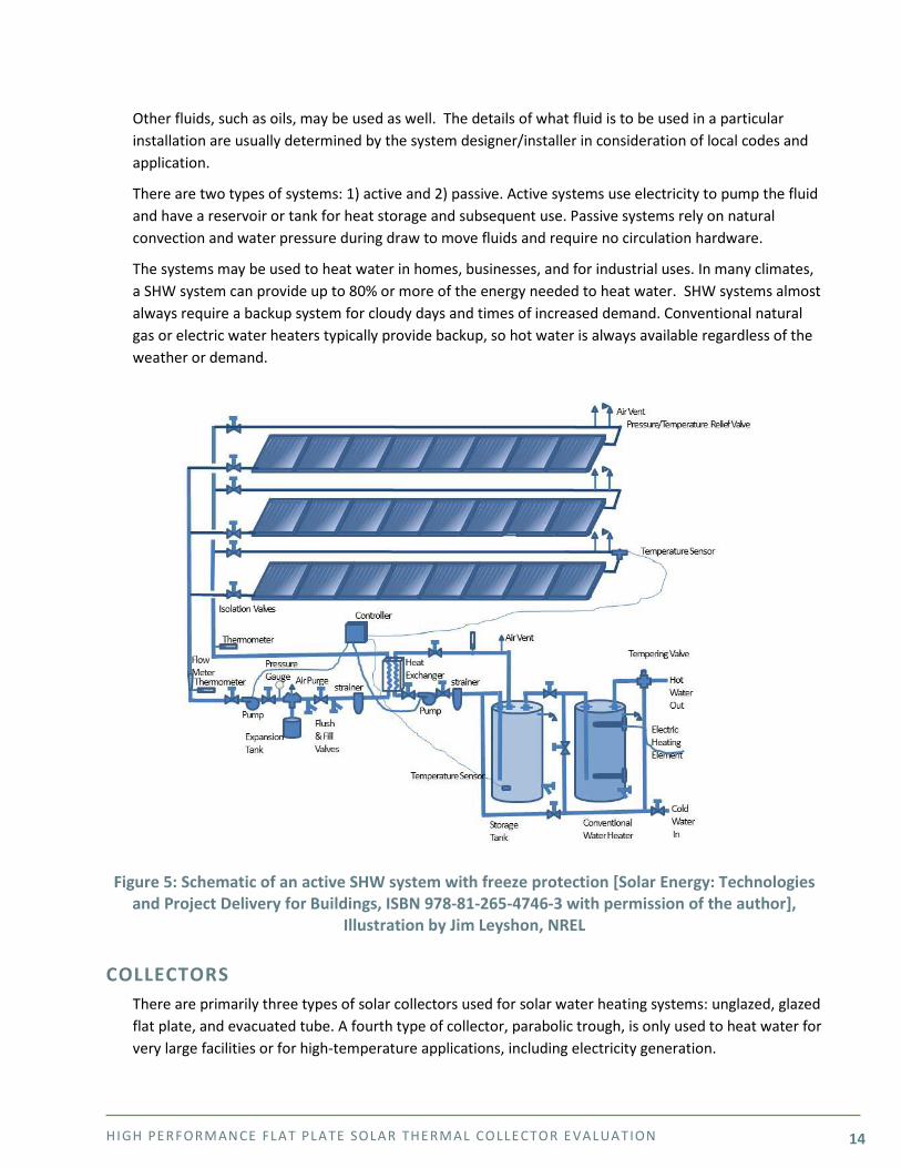
TRADITIONAL SOLAR HOT WATER Solar water heating systems use solar collectors to capture sunlight to heat a fluid. The heat from the collector fluid is then moved to the fluid in a solar storage, or preheat, tank, or in some cases supplied directly to the hot water load (Figure 5). Various fluids are used in solar thermal systems in consideration of their application. Water with a concentration of propylene glycol is typical for most applications where freeze protection is needed. Typical concentrations of glycol range from 20% up to 50% or more in colder climates. Solar thermal systems in warm climates may use water only.
HIGH PE RFORMANCE FLAT PLATE SOLAR THE RMAL COLLE CTOR E VALUATION 14
Other fluids, such as oils, may be used as well. The details of what fluid is to be used in a particular installation are usually determined by the system designer/installer in consideration of local codes and application.
There are two types of systems: 1) active and 2) passive. Active systems use electricity to pump the fluid and have a reservoir or tank for heat storage and subsequent use. Passive systems rely on natural convection and water pressure during draw to move fluids and require no circulation hardware.
The systems may be used to heat water in homes, businesses, and for industrial uses. In many climates, a SHW system can provide up to 80% or more of the energy needed to heat water. SHW systems almost always require a backup system for cloudy days and times of increased demand. Conventional natural gas or electric water heaters typically provide backup, so hot water is always available regardless of the weather or demand.
Figure 5: Schematic of an active SHW system with freeze protection [Solar Energy: Technologies and Project Delivery for Buildings, ISBN 978-81-265-4746-3 with permission of the author],
Illustration by Jim Leyshon, NREL
COLLECTORS There are primarily three types of solar collectors used for solar water heating systems: unglazed, glazed flat plate, and evacuated tube. A fourth type of collector, parabolic trough, is only used to heat water for very large facilities or for high-temperature applications, including electricity generation.
HIGH PE RFORMANCE FLAT PLATE SOLAR THE RMAL COLLE CTOR E VALUATION 15
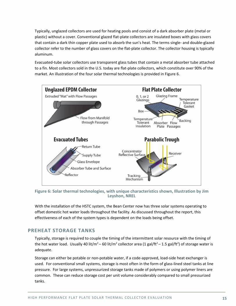
Typically, unglazed collectors are used for heating pools and consist of a dark absorber plate (metal or plastic) without a cover. Conventional glazed flat-plate collectors are insulated boxes with glass covers that contain a dark thin copper plate used to absorb the sun’s heat. The terms single- and double-glazed collector refer to the number of glass covers on the flat-plate collector. The collector housing is typically aluminum.
Evacuated-tube solar collectors use transparent glass tubes that contain a metal absorber tube attached to a fin. Most collectors sold in the U.S. today are flat-plate collectors, which constitute over 90% of the market. An illustration of the four solar thermal technologies is provided in Figure 6.
Figure 6: Solar thermal technologies, with unique characteristics shown, Illustration by Jim
Leyshon, NREL
With the installation of the HSTC system, the Bean Center now has three solar systems operating to offset domestic hot water loads throughout the facility. As discussed throughout the report, this effectiveness of each of the system types is dependent on the loads being offset.
PREHEAT STORAGE TANKS Typically, storage is required to couple the timing of the intermittent solar resource with the timing of the hot water load. Usually 40 lit/m2 – 60 lit/m2 collector area (1 gal/ft2 – 1.5 gal/ft2) of storage water is adequate.
Storage can either be potable or non-potable water, if a code-approved, load-side heat exchanger is used. For conventional small systems, storage is most often in the form of glass-lined steel tanks at line pressure. For large systems, unpressurized storage tanks made of polymers or using polymer liners are common. These can reduce storage cost per unit volume considerably compared to small pressurized tanks.
HIGH PE RFORMANCE FLAT PLATE SOLAR THE RMAL COLLE CTOR E VALUATION 16
AUXILIARY TANKS Auxiliary tanks are conventional domestic water heaters served by electricity or natural gas and provide the required energy to meet the domestic water heading requirements not offset by the solar thermal system.
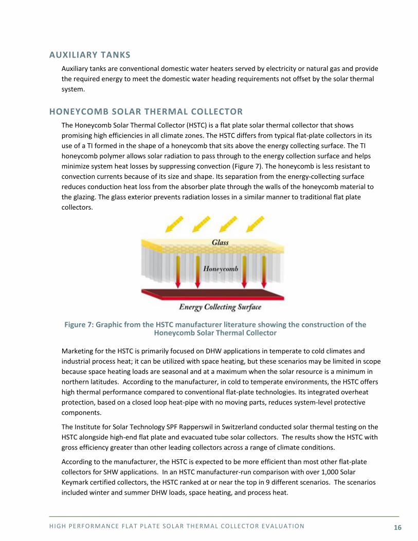
HONEYCOMB SOLAR THERMAL COLLECTOR The Honeycomb Solar Thermal Collector (HSTC) is a flat plate solar thermal collector that shows promising high efficiencies in all climate zones. The HSTC differs from typical flat-plate collectors in its use of a TI formed in the shape of a honeycomb that sits above the energy collecting surface. The TI honeycomb polymer allows solar radiation to pass through to the energy collection surface and helps minimize system heat losses by suppressing convection (Figure 7). The honeycomb is less resistant to convection currents because of its size and shape. Its separation from the energy-collecting surface reduces conduction heat loss from the absorber plate through the walls of the honeycomb material to the glazing. The glass exterior prevents radiation losses in a similar manner to traditional flat plate collectors.
Figure 7: Graphic from the HSTC manufacturer literature showing the construction of the
Honeycomb Solar Thermal Collector
Marketing for the HSTC is primarily focused on DHW applications in temperate to cold climates and industrial process heat; it can be utilized with space heating, but these scenarios may be limited in scope because space heating loads are seasonal and at a maximum when the solar resource is a minimum in northern latitudes. According to the manufacturer, in cold to temperate environments, the HSTC offers high thermal performance compared to conventional flat-plate technologies. Its integrated overheat protection, based on a closed loop heat-pipe with no moving parts, reduces system-level protective components.
The Institute for Solar Technology SPF Rapperswil in Switzerland conducted solar thermal testing on the HSTC alongside high-end flat plate and evacuated tube solar collectors. The results show the HSTC with gross efficiency greater than other leading collectors across a range of climate conditions.
According to the manufacturer, the HSTC is expected to be more efficient than most other flat-plate collectors for SHW applications. In an HSTC manufacturer-run comparison with over 1,000 Solar Keymark certified collectors, the HSTC ranked at or near the top in 9 different scenarios. The scenarios included winter and summer DHW loads, space heating, and process heat.
HIGH PE RFORMANCE FLAT PLATE SOLAR THE RMAL COLLE CTOR E VALUATION 17
The analysis looked specifically at the area-weighted (kW/m2) output of the solar collectors. It is important to note, however, that comparing the energy output on the basis of gross area is potentially misleading because the important figure of merit for a SHW system is delivered energy cost. A system using less thermally efficient collectors may have a lower installed cost, which offsets the lower amount of energy being collected.
In October 2012, the HSTC collector earned the Solar Keymark European certification Q4-12. This quality assurance designation with the European Committee for Standardization guarantees the quality of solar thermal products in the European Union (EU). The Solar Keymark certification is the primary certification authority for solar thermal products in the EU. The HSTC qualifies for EU government subsidies, which help to reduce costs in the EU.
III. Methodology
A. Technical Objectives The HSTC’s overall performance was evaluated at the Major General Emmett J. Bean Center (hereinafter, Bean Center) in Indianapolis, IN, and at the GSA Regional Headquarters Building (hereinafter, Auburn Site) in Auburn, WA. The first technical objective focuses on ensuring the collector performance is within ±10% of the manufacturer-provided performance curve. The second objective focuses on analyzing the collector’s overall efficiency relative to incumbent technologies. The third objective focuses on confirming that the HSTC’s overheat protection device (OPD) operates as expected. The remaining objectives analyze the Life-Cycle costs of the product versus incumbent technologies, and the return on investment at the demonstration facilities. Specific quantitative performance objectives are outlined in Table 2.
HIGH PE RFORMANCE FLAT PLATE SOLAR THE RMAL COLLE CTOR E VALUATION 18
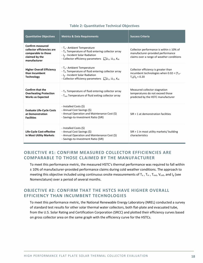
Table 2: Quantitative Technical Objectives
Quantitative Objectives Metrics & Data Requirements Success Criteria
Confirm measured collector efficiencies are comparable to those claimed by the manufacturer
- Ta - Ambient Temperature - Tin Temperature of fluid entering collector array - Ig - Incident Solar Radiation - Collector efficiency parameters 0, UL1, UL2, KIA
Collector performance is within ± 10% of manufacturer-provided performance claims over a range of weather conditions
Higher Overall Efficiency than Incumbent Technology
- Ta - Ambient Temperature - Tin Temperature of fluid entering collector array - Ig - Incident Solar Radiation - Collector efficiency parameters 0, UL1, UL2, KIA
Collector efficiency is greater than incumbent technologies when 0.02 < (Tm-Ta)/Ig < 0.20
Confirm that the Overheating Protection Works as Expected
- Tin Temperature of fluid entering collector array - Tout Temperature of fluid exiting collector array
Measured collector stagnation temperatures do not exceed those predicted by the HSTC manufacturer
Evaluate Life-Cycle Costs at Demonstration Facilities
- Installed Costs ($) - Annual Cost Savings ($) - Annual Operation and Maintenance Cost ($) - Savings-to-Investment Ratio (SIR)
SIR > 1 at demonstration facilities
Life-Cycle Cost-effective in Most Utility Markets
- Installed Costs ($) - Annual Cost Savings ($) - Annual Operation and Maintenance Cost ($) - Savings-to-Investment Ratio (SIR)
SIR > 1 in most utility markets/ building characteristics
OBJECTIVE #1: CONFIRM MEASURED COLLECTOR EFFICIENCIES ARE COMPARABLE TO THOSE CLAIMED BY THE MANUFACTURER
To meet this performance metric, the measured HSTC’s thermal performance was required to fall within ± 10% of manufacturer-provided performance claims during cold weather conditions. The approach to meeting this objective included using continuous onsite measurements of Ta , Tin , Tout, Vcoll, and Ig (see Nomenclature) over a period of several months.
OBJECTIVE #2: CONFIRM THAT THE HSTCS HAVE HIGHER OVERALL EFFICIENCY THAN INCUMBENT TECHNOLOGIES
To meet this performance metric, the National Renewable Energy Laboratory (NREL) conducted a survey of standard test results for other solar thermal water collectors, both flat-plate and evacuated tube, from the U.S. Solar Rating and Certification Corporation (SRCC) and plotted their efficiency curves based on gross collector area on the same graph with the efficiency curve for the HSTCs.

HIGH PE RFORMANCE FLAT PLATE SOLAR THE RMAL COLLE CTOR E VALUATION 19
OBJECTIVE #3: CONFIRM THAT THE OVERHEATING PROTECTION OF THE HSTC WORKS AS EXPECTED
At the Bean Center, where the most trusted data acquisition system is installed, O&M personnel shut off the solar fluid pump and let the collector array stagnate during several clear days. NREL compared the measured fluid temperature at the outlet of the array to the temperature limit predicted by the HSTC manufacturer. If the measured temperatures did not exceed the predicted temperatures by more than 5oC and no apparent damage was caused to the collectors, the objective of confirming overheating protection is working would be confirmed.
OBJECTIVE #4: LIFE-CYCLE COST-EFFECTIVE AT DEMONSTRATION FACILITIES
Annual energy savings and life-cycle costs were analyzed at each facility based on measured data from the each site.
OBJECTIVE #5: COMPARE LIFE-CYCLE COST-EFFECTIVENESS OF HSTC TO STANDARD FLAT PLATE OVER A RANGE OF CLIMATES
Annual energy savings were predicted using TRNSYS [2], a sub-hourly simulation tool. NREL ran a series of simulations with a range of loads, geographic locations, and installed costs to provide an assessment of how HSTC systems compare in overall lifetime cost to systems employing standard flat-plate collectors.
B. Criteria for Site selection The specific site selection criteria that were created to ensure an effective evaluation of the HSTCs are outlined below.
FAVORABLE CLIMATIC CONDITIONS Two demonstration sites were selected and hosted by GSA: the (Bean Center) in Indianapolis, Indiana, GSA Region 5 and the GSA Regional Headquarters Building in Auburn, Washington, GSA Region 10. These locations were selected based on their local climatic conditions, which are characterized by diffuse light conditions in the winter and colder seasons, variable summer solar resource, and cold winters. These climatic conditions provided a means for testing the technology claims of high operating efficiencies in cold climates.
FULLY OPERATIONAL BASELINE AND SUFFICIENT DOMESTIC HOT WATER LOAD
The baseline water heating system was specified to be fully functioning and operating in the same manner as the water heating system being evaluated after the installation of the solar thermal collector system.
HIGH PE RFORMANCE FLAT PLATE SOLAR THE RMAL COLLE CTOR E VALUATION 20
Each site is primarily of office space type occupancy. While the Auburn site initially had a significant DHW load due to an operational cafeteria, the cafeteria load was removed when the cafeteria was closed.
STABLE CONDITIONS FOR MEASUREMENT The site conditions were specified to be the same for both the baseline and the post-installation testing. Changes in occupants, building operation, or potential site conditions could affect the results and may make comparative measurements difficult.
AVAILABLE ROOF AREA AND SOLAR ACCESS Each site had sufficient roof area available with the Bean Center already hosting numerous solar energy technologies, including multiple solar photovoltaic (PV) technologies, along with traditional flat plate and evacuated tube solar thermal technologies. The Auburn facility has no other renewable energy systems installed at the site.
IV. Measurement & Verification Evaluation Plan
A. Facility Description The HSTC’s overall performance was evaluated at the Bean Center in Indianapolis, IN, and at the GSA Regional Headquarters Building in GSA facility in Auburn, WA. Building information and water heating system descriptions for each site are provided in Table 3.
Table 3: Building Information and Water Heating System Descriptions
Building Location Building Area (GSF)
Primary Water Heating System End-use
GSA Regional HQ Auburn, WA 105,771 Electric (originally natural gas) DHW
Bean Center Indianapolis Indianapolis, IN 1,600,000 Electric DHW
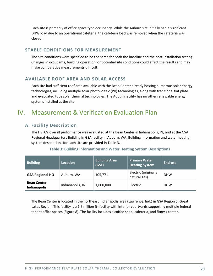
The Bean Center is located in the northeast Indianapolis area (Lawrence, Ind.) in GSA Region 5, Great Lakes Region. This facility is a 1.6 million ft2 facility with interior courtyards supporting multiple federal tenant office spaces (Figure 8). The facility includes a coffee shop, cafeteria, and fitness center.
HIGH PE RFORMANCE FLAT PLATE SOLAR THE RMAL COLLE CTOR E VALUATION 21
Figure 8: Bean Center Site
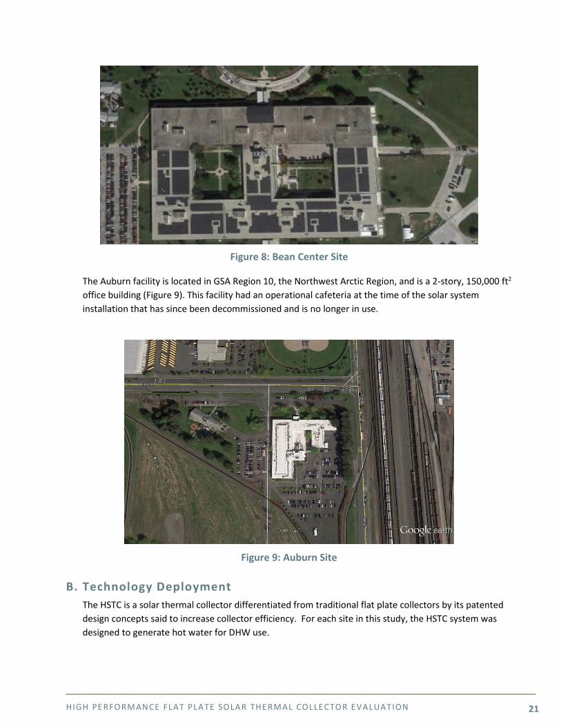
The Auburn facility is located in GSA Region 10, the Northwest Arctic Region, and is a 2-story, 150,000 ft2 office building (Figure 9). This facility had an operational cafeteria at the time of the solar system installation that has since been decommissioned and is no longer in use.
Figure 9: Auburn Site
B. Technology Deployment The HSTC is a solar thermal collector differentiated from traditional flat plate collectors by its patented design concepts said to increase collector efficiency. For each site in this study, the HSTC system was designed to generate hot water for DHW use.

HIGH PE RFORMANCE FLAT PLATE SOLAR THE RMAL COLLE CTOR E VALUATION 22
BEAN CENTER The main components of the solar hot water heating system at the Bean Center (Figure 12) are:
• Closed-Loop System – The system is designed as a standard closed loop system, where a pump circulates a water/propylene glycol mixture through the collectors and an external heat exchanger.
• HSTCs – A total of eight HSTC modules were installed at the Bean Center, with two sets of four modules plumbed in series. Each set of four modules are plumbed in parallel.
• Preheat Tank – There are a total of three preheat tanks that store heated water from the solar thermal collectors and preheat the domestic hot water before it is supplied to the auxiliary tanks. As shown in Figure 13, the preheat tanks are heated solely by the collector array.
• Auxiliary Tank – The Bean Center DHW system uses a standard 454-liter (120-gallon) storage type electric water heater that serves the southeast portion of the facility. Pre-heated water from the preheat tanks is fed to the auxiliary tank where it is heated to the hot water delivery setpoint, if necessary, and supplied to the facility. While the Bean Center does have a functional cafeteria, the load being served by the eight-panel HSTC system consists primarily of lavatory end uses in the restrooms.
• External Heat Exchanger – An external heat exchanger transfers heat from the solar collectors to the pre-heat tanks.
• Solar Pump Station – Circulation pumps circulate water through the solar thermal loop and the external heat exchanger. A separate set of pumps circulate fluid from the pre-heat tanks to external heat exchangers.
• Solar Controller –Under normal operations at the Bean Center, the circulating pumps serving the solar collectors and the solar storage tanks are started when the collector temperature exceeds the solar tank storage by 20°F and stopped when the collector temperature is less than 5°F higher than the solar storage tank lower temperature.
• Installed Costs – The installed system cost of the eight-panel system at the Bean Center is $64,670.
A photo of the eight-panel HSTC installation at the Bean center is provided in Figure 10.

HIGH PE RFORMANCE FLAT PLATE SOLAR THE RMAL COLLE CTOR E VALUATION 23
Figure 10: Bean Center HSTC Installation. Photo credit Caleb Rockenbaugh, NREL.
AUBURN SITE The main components of the combined DHW and solar thermal system at the Auburn site (Figure 13) are:
• Recirculation Loop System –Rather than preheating the cold mains water when it enters the facility, this system reheats DHW in a recirculation loop. In this case, the temperature of the water entering the solar storage tank is much warmer than the mains water. Heating water that is returning in a recirculation loop would not be practical with most flat-plate collectors since their efficiency would be low at the loop’s elevated temperatures. This is potentially a good application for the HSTCs because they perform well at higher temperatures.
• HSTCs – A total of four HSTC modules were installed at the Auburn site. The system was plumbed with all panels running in parallel.
• Solar Storage Tank – There is one storage tank with an internal heat exchanger that reheats DHW returning from the circulation loop before it is reintroduced to the loop.
• Solar Pump Station – Pump circulates aqueous propylene glycol solution through the solar thermal loop and the solar storage tank.
• Solar Controller –Under normal operations at the Auburn site, the circulating pumps serving the solar collectors are started when the collector temperature exceeds the solar tank storage by 20°F and stopped when the collector temperature is less than 5°F higher than the solar storage tank’s lower temperature.
• Installed Costs – The installed system cost of the four-panel system at the Auburn site is $81,950.
A photo of the four HSTCs installed at the Auburn site is provided in Figure 11.

HIGH PE RFORMANCE FLAT PLATE SOLAR THE RMAL COLLE CTOR E VALUATION 24
Figure 11: Auburn HSTC System Installation. Photo credit Caleb Rockenbaugh, NREL.
C. Measurement and Verification In this study, the purpose of the field measurements was to verify the performance of the HSTCs in comparison to the HSTC manufacturer’s claimed values. The balance of the system—pumps, pipes, storage tanks—is standard equipment used in any SHW system and their performance is not in question.
At both sites, measurements were made using a Campbell Scientific CR1000 data logger. Measurements were sampled at a frequency of 1 second and averaged over data storage intervals of 1, 15, and 60 minutes.
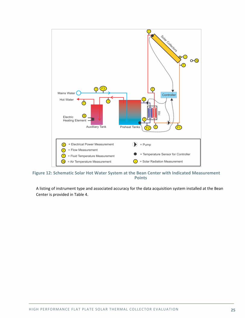
BEAN CENTER A schematic of the SHW system currently installed at the Bean Center, with measurement points indicated, is provided in Figure 6. All fluid temperatures were measured using type T thermocouples immersed in the fluid. A pyranometer (solar radiation sensor) was mounted in the plane of the collector array. Outdoor air temperature was measured in a passive radiation shield.
HIGH PE RFORMANCE FLAT PLATE SOLAR THE RMAL COLLE CTOR E VALUATION 25
Figure 12: Schematic Solar Hot Water System at the Bean Center with Indicated Measurement
Points
A listing of instrument type and associated accuracy for the data acquisition system installed at the Bean Center is provided in Table 4.
HIGH PE RFORMANCE FLAT PLATE SOLAR THE RMAL COLLE CTOR E VALUATION 26
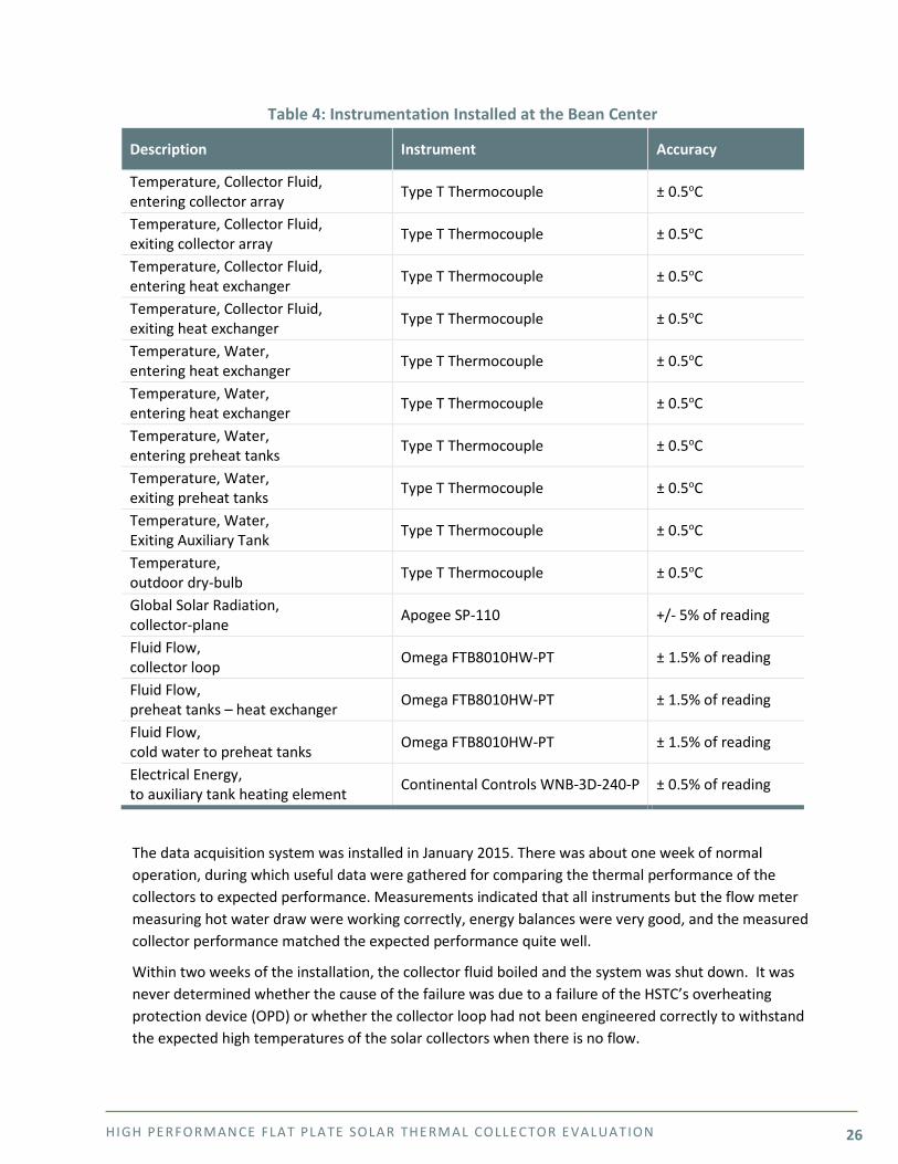
Table 4: Instrumentation Installed at the Bean Center
Description Instrument Accuracy
Temperature, Collector Fluid, entering collector array Type T Thermocouple ± 0.5oC
Temperature, Collector Fluid, exiting collector array Type T Thermocouple ± 0.5oC
Temperature, Collector Fluid, entering heat exchanger Type T Thermocouple ± 0.5oC
Temperature, Collector Fluid, exiting heat exchanger Type T Thermocouple ± 0.5oC
Temperature, Water, entering heat exchanger Type T Thermocouple ± 0.5oC
Temperature, Water, entering heat exchanger Type T Thermocouple ± 0.5oC
Temperature, Water, entering preheat tanks Type T Thermocouple ± 0.5oC
Temperature, Water, exiting preheat tanks Type T Thermocouple ± 0.5oC
Temperature, Water, Exiting Auxiliary Tank Type T Thermocouple ± 0.5oC
Temperature, outdoor dry-bulb Type T Thermocouple ± 0.5oC
Global Solar Radiation, collector-plane Apogee SP-110 +/- 5% of reading
Fluid Flow, collector loop Omega FTB8010HW-PT ± 1.5% of reading
Fluid Flow, preheat tanks – heat exchanger Omega FTB8010HW-PT ± 1.5% of reading
Fluid Flow, cold water to preheat tanks Omega FTB8010HW-PT ± 1.5% of reading
Electrical Energy, to auxiliary tank heating element Continental Controls WNB-3D-240-P ± 0.5% of reading
The data acquisition system was installed in January 2015. There was about one week of normal operation, during which useful data were gathered for comparing the thermal performance of the collectors to expected performance. Measurements indicated that all instruments but the flow meter measuring hot water draw were working correctly, energy balances were very good, and the measured collector performance matched the expected performance quite well.
Within two weeks of the installation, the collector fluid boiled and the system was shut down. It was never determined whether the cause of the failure was due to a failure of the HSTC’s overheating protection device (OPD) or whether the collector loop had not been engineered correctly to withstand the expected high temperatures of the solar collectors when there is no flow.
HIGH PE RFORMANCE FLAT PLATE SOLAR THE RMAL COLLE CTOR E VALUATION 27
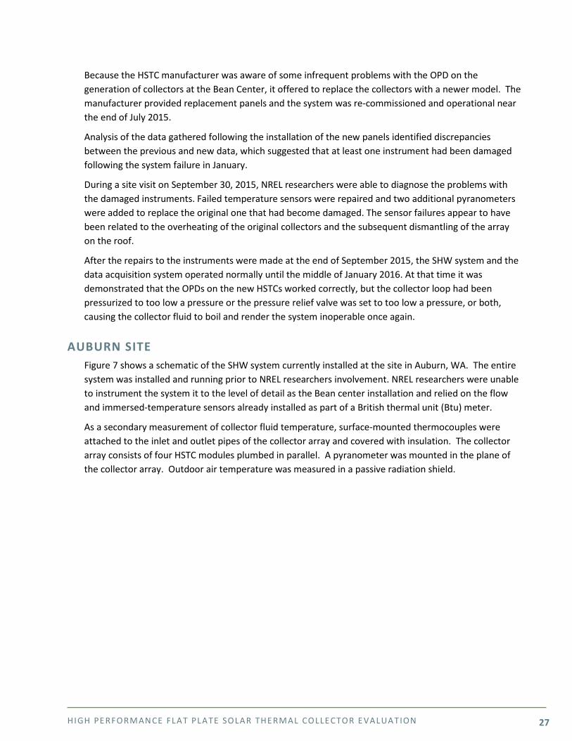
Because the HSTC manufacturer was aware of some infrequent problems with the OPD on the generation of collectors at the Bean Center, it offered to replace the collectors with a newer model. The manufacturer provided replacement panels and the system was re-commissioned and operational near the end of July 2015.
Analysis of the data gathered following the installation of the new panels identified discrepancies between the previous and new data, which suggested that at least one instrument had been damaged following the system failure in January.
During a site visit on September 30, 2015, NREL researchers were able to diagnose the problems with the damaged instruments. Failed temperature sensors were repaired and two additional pyranometers were added to replace the original one that had become damaged. The sensor failures appear to have been related to the overheating of the original collectors and the subsequent dismantling of the array on the roof.
After the repairs to the instruments were made at the end of September 2015, the SHW system and the data acquisition system operated normally until the middle of January 2016. At that time it was demonstrated that the OPDs on the new HSTCs worked correctly, but the collector loop had been pressurized to too low a pressure or the pressure relief valve was set to too low a pressure, or both, causing the collector fluid to boil and render the system inoperable once again.
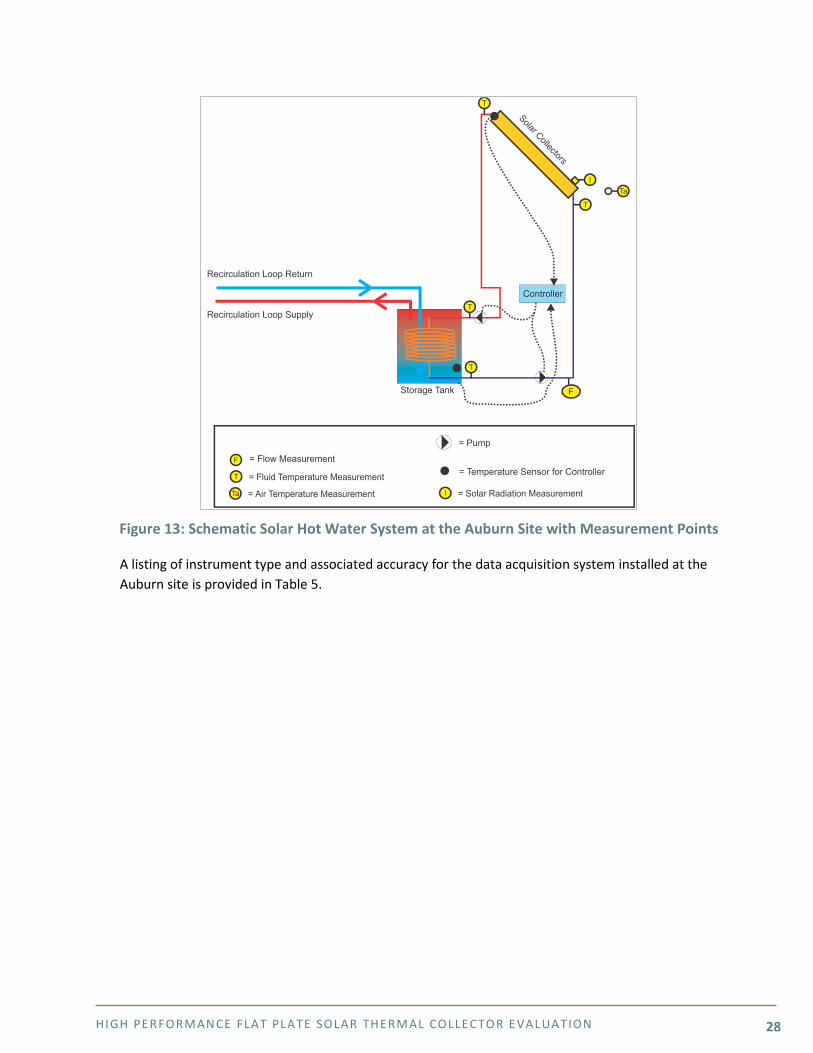
AUBURN SITE Figure 7 shows a schematic of the SHW system currently installed at the site in Auburn, WA. The entire system was installed and running prior to NREL researchers involvement. NREL researchers were unable to instrument the system it to the level of detail as the Bean center installation and relied on the flow and immersed-temperature sensors already installed as part of a British thermal unit (Btu) meter.
As a secondary measurement of collector fluid temperature, surface-mounted thermocouples were attached to the inlet and outlet pipes of the collector array and covered with insulation. The collector array consists of four HSTC modules plumbed in parallel. A pyranometer was mounted in the plane of the collector array. Outdoor air temperature was measured in a passive radiation shield.
HIGH PE RFORMANCE FLAT PLATE SOLAR THE RMAL COLLE CTOR E VALUATION 28
Figure 13: Schematic Solar Hot Water System at the Auburn Site with Measurement Points
A listing of instrument type and associated accuracy for the data acquisition system installed at the Auburn site is provided in Table 5.
HIGH PE RFORMANCE FLAT PLATE SOLAR THE RMAL COLLE CTOR E VALUATION 29
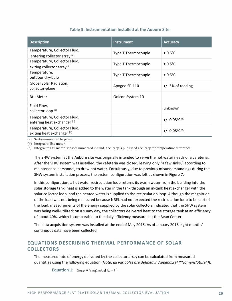
Table 5: Instrumentation Installed at the Auburn Site
Description Instrument Accuracy
Temperature, Collector Fluid, entering collector array (a)
Type T Thermocouple ± 0.5oC
Temperature, Collector Fluid, exiting collector array (a)
Type T Thermocouple ± 0.5oC
Temperature, outdoor dry-bulb Type T Thermocouple ± 0.5oC
Global Solar Radiation, collector-plane Apogee SP-110 +/- 5% of reading
Btu Meter Onicon System 10
Fluid Flow, collector loop (b) unknown
Temperature, Collector Fluid, entering heat exchanger (b) +/- 0.08oC (c)
Temperature, Collector Fluid, exiting heat exchanger (b) +/- 0.08oC (c)
(a) Surface-mounted to pipes (b) Integral to Btu meter (c) Integral to Btu meter, sensors immersed in fluid. Accuracy is published accuracy for temperature difference
The SHW system at the Auburn site was originally intended to serve the hot water needs of a cafeteria. After the SHW system was installed, the cafeteria was closed, leaving only “a few sinks,” according to maintenance personnel, to draw hot water. Fortuitously, due to previous misunderstandings during the SHW system installation process, the system configuration was left as shown in Figure 7.
In this configuration, a hot water recirculation loop returns its warm water from the building into the solar storage tank, heat is added to the water in the tank through an in-tank heat exchanger with the solar collector loop, and the heated water is supplied to the recirculation loop. Although the magnitude of the load was not being measured because NREL had not expected the recirculation loop to be part of the load, measurements of the energy supplied by the solar collectors indicated that the SHW system was being well-utilized; on a sunny day, the collectors delivered heat to the storage tank at an efficiency of about 40%, which is comparable to the daily efficiency measured at the Bean Center.
The data acquisition system was installed at the end of May 2015. As of January 2016 eight months’ continuous data have been collected.
EQUATIONS DESCRIBING THERMAL PERFORMANCE OF SOLAR COLLECTORS
The measured rate of energy delivered by the collector array can be calculated from measured quantities using the following equation (Note: all variables are defined in Appendix H (“Nomenclature”)):
Equation 1: qcoll,m = VcollρcollCp(To – Ti)
HIGH PE RFORMANCE FLAT PLATE SOLAR THE RMAL COLLE CTOR E VALUATION 30
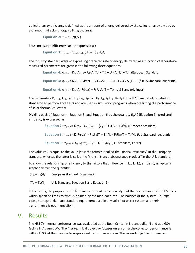
Collector array efficiency is defined as the amount of energy delivered by the collector array divided by the amount of solar energy striking the array:
Equation 2: η = qcoll/(IgAc)
Thus, measured efficiency can be expressed as:
Equation 3: ηmeas = VcollρcollCp(To – Ti) / (IgAc)
The industry-standard ways of expressing predicted rate of energy delivered as a function of laboratory-measured parameters are given in the following three equations:
Equation 4: qcoll,p = KiaIgAcη0 – UL1Ac(Tm – Ta) – UL2 Ac(Tm – Ta)2 (European Standard)
Equation 5: qcoll,p = KiaIgAc FR(τα) – FR UL1Ac(Ti – Ta) – FR UL2 Ac(Ti – Ta)2 (U.S Standard, quadratic)
Equation 6: qcoll,p = KiaIgAc FR(τα) – FR ULAc(Ti – Ta) (U.S Standard, linear)
The parameters Kia, η0, UL1, and UL2 (Kia, FR(τα), FR UL1, FR UL2, FR UL in the U.S.) are calculated during standardized performance tests and are used in simulation programs when predicting the performance of solar thermal collectors.
Dividing each of Equation 4, Equation 5, and Equation 6 by the quantity (IgAc) (Equation 2), predicted efficiency is expressed as:
Equation 7: ηpred = Kiaη0 – UL1(Tm – Ta)/Ig – UL2(Tm – Ta)2/Ig (European Standard)
Equation 8: ηpred = KiaFR(τα) – FRUL1(Ti – Ta)/Ig – FRUL2(Ti – Ta)2/Ig (U.S Standard, quadratic)
Equation 9: ηpred = KiaFR(τα) – FRUL(Ti – Ta)/Ig (U.S Standard, linear)
The value (η0) is equal to the value (τα); the former is called the “optical efficiency” in the European standard, whereas the latter is called the “transmittance-absorptance product” in the U.S. standard.
To show the relationship of efficiency to the factors that influence it (Tm, Ta, Ig), efficiency is typically graphed versus the quantity:
(Tm – Ta)/Ig (European Standard, Equation 7)
(Tin – Ta)/Ig (U.S. Standard, Equation 8 and Equation 9)
In this study, the purpose of the field measurements was to verify that the performance of the HSTCs is within specified limits to what is claimed by the manufacturer. The balance of the system—pumps, pipes, storage tanks—are standard equipment used in any solar hot water system and their performance is not in question.
V. Results The HSTC’s thermal performance was evaluated at the Bean Center in Indianapolis, IN and at a GSA facility in Auburn, WA. The first technical objective focuses on ensuring the collector performance is within ±10% of the manufacturer-provided performance curve. The second objective focuses on
HIGH PE RFORMANCE FLAT PLATE SOLAR THE RMAL COLLE CTOR E VALUATION 31
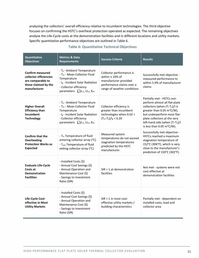
analyzing the collectors’ overall efficiency relative to incumbent technologies. The third objective focuses on confirming the HSTC’s overheat protection operated as expected. The remaining objectives analyze the Life-Cycle costs at the demonstration facilities and in different locations and utility markets. Specific quantitative performance objectives are outlined in Table 6.
Table 6: Quantitative Technical Objectives
Quantitative Objectives
Metrics & Data Requirements Success Criteria Results
Confirm measured collector efficiencies are comparable to those claimed by the manufacturer
- Ta - Ambient Temperature - Tm - Mean Collector Fluid Temperature - Ig - Incident Solar Radiation - Collector efficiency parameters 0, UL1, UL2, KIA
Collector performance is within ± 10% of manufacturer provided performance claims over a range of weather conditions
Successfully met objective - measured performance to within 5.9% of manufacturer claims
Higher Overall Efficiency than Incumbent Technology
- Ta - Ambient Temperature - Tm - Mean Collector Fluid Temperature - Ig - Incident Solar Radiation - Collector efficiency parameters 0, UL1, UL2, KIA
Collector efficiency is greater than incumbent technologies when 0.02 < (Tm-Ta)/Ig < 0.20
Partially met - HSTCs out-perform almost all flat-plate collectors (when (Ti-Ta)/I is greater than 0.05 m2C/W), but underperform most flat-plate collectors at the very left-hand side (when (Ti-Ta)/I is less than 0.05 m2C/W).
Confirm that the Overheating Protection Works as Expected
- Tin Temperature of fluid entering collector array (oC) - Tout Temperature of fluid exiting collector array (oC)
Measured system temperatures do not exceed stagnation temperatures predicted by the HSTC manufacturer.
Successfully met objective - HSTCs reached a maximum stagnation temperature of 152oC (306oF), which is very close to the manufacturer’s prediction of 150oC (302oF).
Evaluate Life-Cycle Costs at Demonstration Facilities
- Installed Costs ($) - Annual Cost Savings ($) - Annual Operation and Maintenance Cost ($) - Savings to Investment Ratio (SIR)
SIR > 1 at demonstration facilities
Not met - systems were not cost-effective at demonstration facilities
Life-Cycle Cost-effective in Most Utility Markets
- Installed Costs ($) - Annual Cost Savings ($) - Annual Operation and Maintenance Cost ($) - Savings to Investment Ratio (SIR)
SIR > 1 in most cost-effective utility markets / building characteristics
Partially met - dependent on installed costs, load and collector area
HIGH PE RFORMANCE FLAT PLATE SOLAR THE RMAL COLLE CTOR E VALUATION 32
OBJECTIVE #1: CONFIRM MEASURED COLLECTOR EFFICIENCIES ARE COMPARABLE TO THOSE CLAIMED BY THE MANUFACTURER
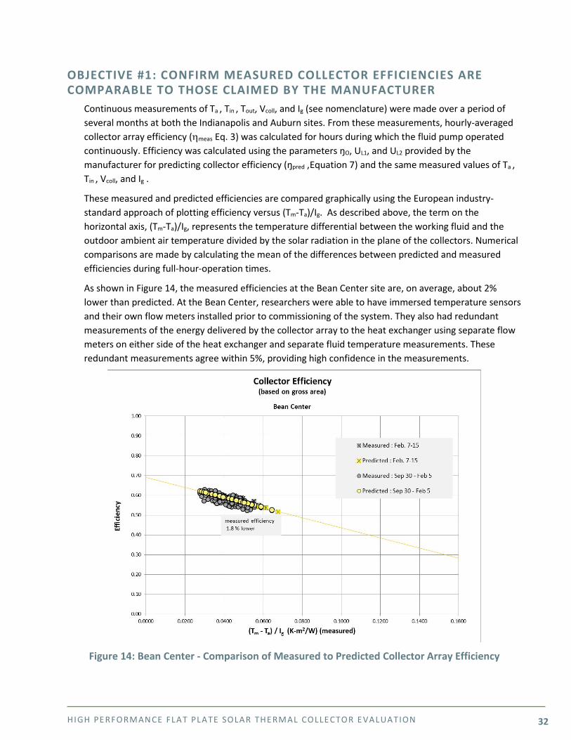
Continuous measurements of Ta , Tin , Tout, Vcoll, and Ig (see nomenclature) were made over a period of several months at both the Indianapolis and Auburn sites. From these measurements, hourly-averaged collector array efficiency (ηmeas Eq. 3) was calculated for hours during which the fluid pump operated continuously. Efficiency was calculated using the parameters ŋO, UL1, and UL2 provided by the manufacturer for predicting collector efficiency (ŋpred ,Equation 7) and the same measured values of Ta , Tin , Vcoll, and Ig .
These measured and predicted efficiencies are compared graphically using the European industry-standard approach of plotting efficiency versus (Tm-Ta)/Ig. As described above, the term on the horizontal axis, (Tm-Ta)/Ig, represents the temperature differential between the working fluid and the outdoor ambient air temperature divided by the solar radiation in the plane of the collectors. Numerical comparisons are made by calculating the mean of the differences between predicted and measured efficiencies during full-hour-operation times.
As shown in Figure 14, the measured efficiencies at the Bean Center site are, on average, about 2% lower than predicted. At the Bean Center, researchers were able to have immersed temperature sensors and their own flow meters installed prior to commissioning of the system. They also had redundant measurements of the energy delivered by the collector array to the heat exchanger using separate flow meters on either side of the heat exchanger and separate fluid temperature measurements. These redundant measurements agree within 5%, providing high confidence in the measurements.
Figure 14: Bean Center - Comparison of Measured to Predicted Collector Array Efficiency
HIGH PE RFORMANCE FLAT PLATE SOLAR THE RMAL COLLE CTOR E VALUATION 33
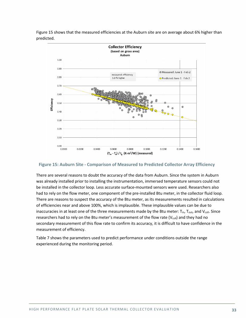
Figure 15 shows that the measured efficiencies at the Auburn site are on average about 6% higher than predicted.
Figure 15: Auburn Site - Comparison of Measured to Predicted Collector Array Efficiency
There are several reasons to doubt the accuracy of the data from Auburn. Since the system in Auburn was already installed prior to installing the instrumentation, immersed temperature sensors could not be installed in the collector loop. Less accurate surface-mounted sensors were used. Researchers also had to rely on the flow meter, one component of the pre-installed Btu meter, in the collector fluid loop. There are reasons to suspect the accuracy of the Btu meter, as its measurements resulted in calculations of efficiencies near and above 100%, which is implausible. These implausible values can be due to inaccuracies in at least one of the three measurements made by the Btu meter: Tin, Tout, and Vcoll. Since researchers had to rely on the Btu meter’s measurement of the flow rate (Vcoll) and they had no secondary measurement of this flow rate to confirm its accuracy, it is difficult to have confidence in the measurement of efficiency.
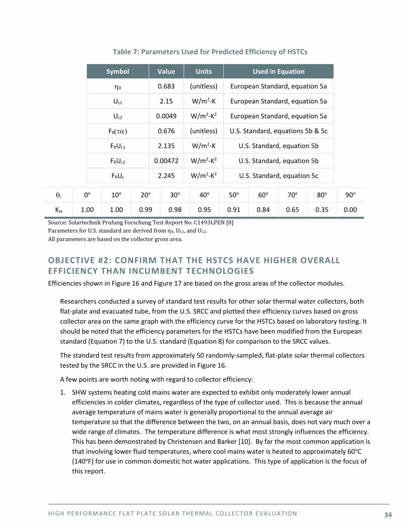
Table 7 shows the parameters used to predict performance under conditions outside the range experienced during the monitoring period.
HIGH PE RFORMANCE FLAT PLATE SOLAR THE RMAL COLLE CTOR E VALUATION 34
Table 7: Parameters Used for Predicted Efficiency of HSTCs
Symbol Value Units Used in Equation
η0 0.683 (unitless) European Standard, equation 5a
UL1 2.15 W/m2-K European Standard, equation 5a
UL2 0.0049 W/m2-K2 European Standard, equation 5a
FR(τα) 0.676 (unitless) U.S. Standard, equations 5b & 5c
FRUL1 2.135 W/m2-K U.S. Standard, equation 5b
FRUL2 0.00472 W/m2-K2 U.S. Standard, equation 5b
FRUL 2.245 W/m2-K2 U.S. Standard, equation 5c
θi 0o 10o 20o 30o 40o 50o 60o 70o 80o 90o
Kia 1.00 1.00 0.99 0.98 0.95 0.91 0.84 0.65 0.35 0.00
Source: Solartechnik Prufung Forschung Test Report No. C1493LPEN [8] Parameters for U.S. standard are derived from η0, UL1, and UL2. All parameters are based on the collector gross area.
OBJECTIVE #2: CONFIRM THAT THE HSTCS HAVE HIGHER OVERALL EFFICIENCY THAN INCUMBENT TECHNOLOGIES Efficiencies shown in Figure 16 and Figure 17 are based on the gross areas of the collector modules.
Researchers conducted a survey of standard test results for other solar thermal water collectors, both flat-plate and evacuated tube, from the U.S. SRCC and plotted their efficiency curves based on gross collector area on the same graph with the efficiency curve for the HSTCs based on laboratory testing. It should be noted that the efficiency parameters for the HSTCs have been modified from the European standard (Equation 7) to the U.S. standard (Equation 8) for comparison to the SRCC values.
The standard test results from approximately 50 randomly-sampled, flat-plate solar thermal collectors tested by the SRCC in the U.S. are provided in Figure 16.
A few points are worth noting with regard to collector efficiency:
1. SHW systems heating cold mains water are expected to exhibit only moderately lower annual efficiencies in colder climates, regardless of the type of collector used. This is because the annual average temperature of mains water is generally proportional to the annual average air temperature so that the difference between the two, on an annual basis, does not vary much over a wide range of climates. The temperature difference is what most strongly influences the efficiency. This has been demonstrated by Christensen and Barker [10]. By far the most common application is that involving lower fluid temperatures, where cool mains water is heated to approximately 60oC (140oF) for use in common domestic hot water applications. This type of application is the focus of this report.

HIGH PE RFORMANCE FLAT PLATE SOLAR THE RMAL COLLE CTOR E VALUATION 35
2. Collectors such as the HSTC, which exhibit higher efficiencies when the difference between inlet fluid temperature and ambient temperature is high, will likely out-perform more conventional collector technologies in applications that run hotter fluid through the collectors. An example of this type of application is one in which the collector array is fed by a hot hydronic loop in a building. In this case the fluid entering the collector is usually close to the hot water set point of 60oC at all times, whereas in the type of application that was simulated for this study the inlet fluid temperature is on average much lower than the set point.
3. For evacuated tube collectors the ratio of gross area to absorber area can vary widely depending on how far apart each tube is from the next. Large spacing results in a large gross area, which results in a low efficiency based on gross area. Many evacuated-tube collectors appear to have much lower efficiencies than flat-plate collectors because the tubes have large spaces between them, which makes the efficiency based on gross area appear low, but is not indicative of overall system performance.
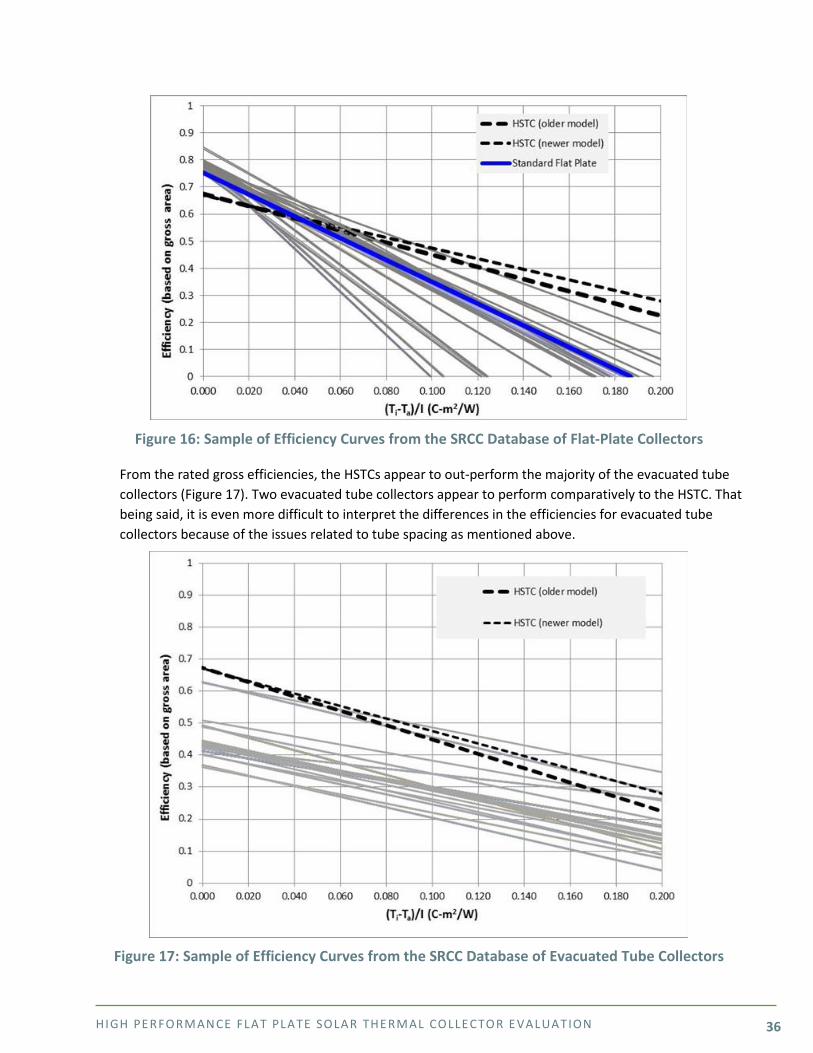
HSTCs out-perform all flat-plate collectors at the right-hand side of Figure 16 (when (Ti-Ta)/I is greater than 0.05), but underperform most flat-plate collectors at the very left-hand side (when (Ti-Ta)/I is less than 0.05). Thus, the HSTC outperforms all flat plate collectors in configurations with higher temperature differences (higher fluid inlet temperatures), but underperforms when the temperature differences are lower (lower fluid inlet temperatures). Note that only one collector in the SRCC database is comparable in performance at higher fluid inlet temperatures to the HSTC; all of the other collectors show potentially lower performance at higher fluid inlet temperatures than the HSTC. Also note that the HSTC manufacturer has developed an improved model (noted as “newer model”) since the analysis of this report was completed, and the improved model promises even higher efficiencies for high fluid temperatures.
Simply comparing efficiency curves, as in Figures 16 and 17, can be deceiving. Exactly where on the graph a collector runs on average is a function of many factors related to the system design. While the temperature differences (Ti-Ta) noted above provide an indication of performance, the life-cycle cost of the entire system, which encompasses the effects of collector efficiency, climate, other system components, energy costs, and installed costs, needs to be considered.
HIGH PE RFORMANCE FLAT PLATE SOLAR THE RMAL COLLE CTOR E VALUATION 36
Figure 16: Sample of Efficiency Curves from the SRCC Database of Flat-Plate Collectors
From the rated gross efficiencies, the HSTCs appear to out-perform the majority of the evacuated tube collectors (Figure 17). Two evacuated tube collectors appear to perform comparatively to the HSTC. That being said, it is even more difficult to interpret the differences in the efficiencies for evacuated tube collectors because of the issues related to tube spacing as mentioned above.
Figure 17: Sample of Efficiency Curves from the SRCC Database of Evacuated Tube Collectors
HIGH PE RFORMANCE FLAT PLATE SOLAR THE RMAL COLLE CTOR E VALUATION 37
OBJECTIVE #3: CONFIRM THAT THE OVER-HEATING PROTECTION OF THE HSTCS WORKS AS EXPECTED
The HSTCs employ a heat pipe as an OPD to prevent the collectors from reaching extremely high temperatures, which can happen if there is no flow through the collectors during a clear day. High collector temperatures are not generally a risk to the collectors themselves, but can result in the breakdown of the collector fluid and other components of the collector loop, such as pumps and seals.
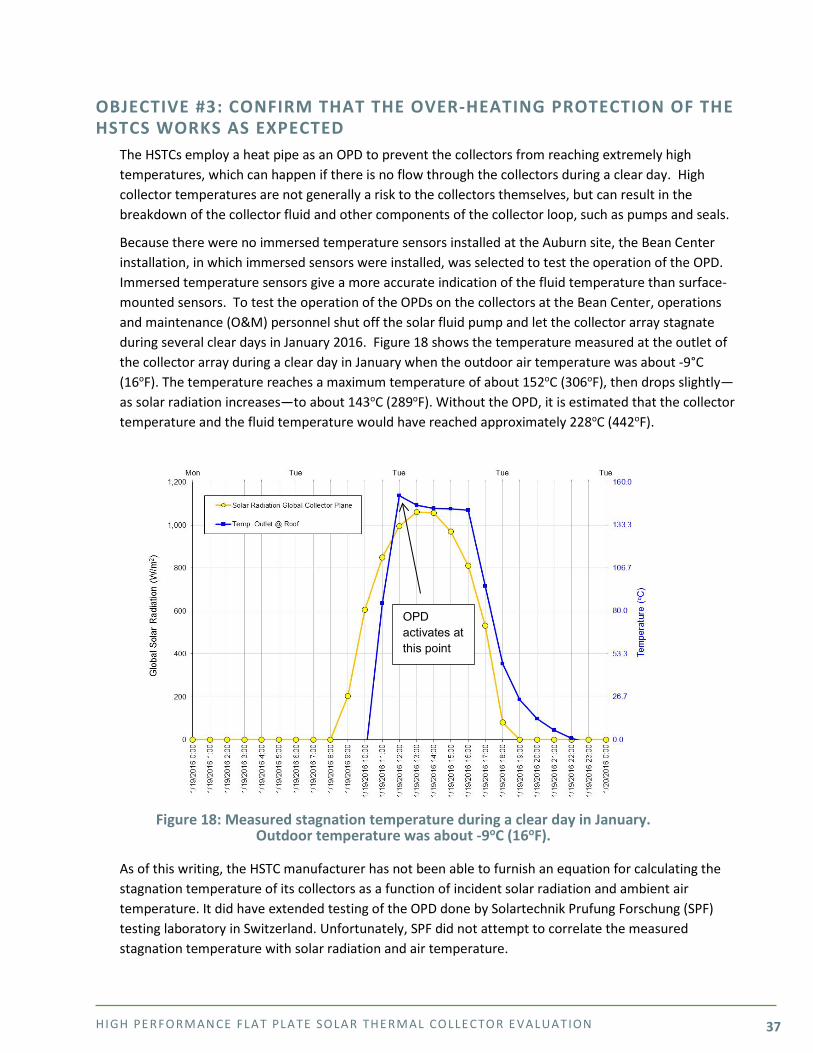
Because there were no immersed temperature sensors installed at the Auburn site, the Bean Center installation, in which immersed sensors were installed, was selected to test the operation of the OPD. Immersed temperature sensors give a more accurate indication of the fluid temperature than surface-mounted sensors. To test the operation of the OPDs on the collectors at the Bean Center, operations and maintenance (O&M) personnel shut off the solar fluid pump and let the collector array stagnate during several clear days in January 2016. Figure 18 shows the temperature measured at the outlet of the collector array during a clear day in January when the outdoor air temperature was about -9°C (16oF). The temperature reaches a maximum temperature of about 152oC (306oF), then drops slightly—as solar radiation increases—to about 143oC (289oF). Without the OPD, it is estimated that the collector temperature and the fluid temperature would have reached approximately 228oC (442oF).
As of this writing, the HSTC manufacturer has not been able to furnish an equation for calculating the stagnation temperature of its collectors as a function of incident solar radiation and ambient air temperature. It did have extended testing of the OPD done by Solartechnik Prufung Forschung (SPF) testing laboratory in Switzerland. Unfortunately, SPF did not attempt to correlate the measured stagnation temperature with solar radiation and air temperature.
OPD activates at this point
Figure 18: Measured stagnation temperature during a clear day in January. Outdoor temperature was about -9oC (16oF).
HIGH PE RFORMANCE FLAT PLATE SOLAR THE RMAL COLLE CTOR E VALUATION 38
SPF did predict a stagnation temperature of 150oC (302oF) with incident solar radiation of 1000 W/m2 and ambient temperature of 0oC (32oF). The stagnation temperature may be a bit higher under higher air temperature conditions. The HSTC manufacturer has assured NREL researchers that the stagnation temperature is not expected to be much higher than 150oC (302oF), under any normal atmospheric conditions. NREL expects to continue monitoring the stagnation temperature at the Bean Center installation through the early part of summer 2016 to confirm this.
The importance of knowing the expected maximum stagnation temperature was illustrated during the experiment at the Bean Center. When the collector temperature rose to 150oC (302oF) the over-pressure safety valve opened and released fluid from the collector loop. This should not happen if the system has been designed correctly.
To design the system correctly, the system designer needs to know the maximum temperature of the collector fluid. Once known, the designer can calculate the pressure to which the collector loop must be pressurized to prevent the fluid from boiling. It is likely that the designers of the system at the Bean Center were unaware of the possible stagnation temperature and filled the loop to too low a pressure or installed a pressure relief device with too low a pressure rating, or both.
OBJECTIVE #4: LIFE-CYCLE COST-EFFECTIVE AT DEMONSTRATION FACILITIES
BEAN CENTER ENERGY SAVINGS AND ECONOMICS Because of the operational problems encountered at the Bean Center within two weeks of the installation of the data acquisition system, reliable data were not collected until the end of September 2015. To predict the annual energy savings from the Bean Center solar hot water system, a TRNSYS simulation model was created. With this design, the water from the storage tanks is heated by circulating a fluid through the solar collectors. This pre-heated water is used as the inlet water to the auxiliary tank. The specifications from the Bean Center solar thermal system were entered directly into the TRNSYS model.
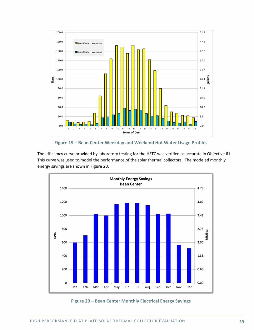
Weekday and weekend hot water draw profiles were created from measurements from the onsite building automation system (BAS). The average weekday and weekend draw profiles are shown in Figure 19.
HIGH PE RFORMANCE FLAT PLATE SOLAR THE RMAL COLLE CTOR E VALUATION 39
Figure 19 – Bean Center Weekday and Weekend Hot Water Usage Profiles
The efficiency curve provided by laboratory testing for the HSTC was verified as accurate in Objective #1. This curve was used to model the performance of the solar thermal collectors. The modeled monthly energy savings are shown in Figure 20.
Figure 20 – Bean Center Monthly Electrical Energy Savings
HIGH PE RFORMANCE FLAT PLATE SOLAR THE RMAL COLLE CTOR E VALUATION 40
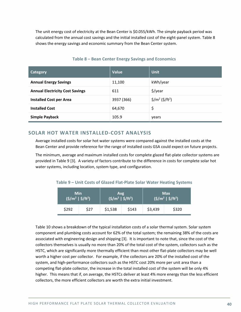
The unit energy cost of electricity at the Bean Center is $0.055/kWh. The simple payback period was calculated from the annual cost savings and the initial installed cost of the eight-panel system. Table 8 shows the energy savings and economic summary from the Bean Center system.
Table 8 – Bean Center Energy Savings and Economics
Category Value Unit
Annual Energy Savings 11,100 kWh/year
Annual Electricity Cost Savings 611 $/year
Installed Cost per Area 3937 (366) $/m2 ($/ft2)
Installed Cost 64,670 $
Simple Payback 105.9 years
SOLAR HOT WATER INSTALLED-COST ANALYSIS Average installed costs for solar hot water systems were compared against the installed costs at the Bean Center and provide reference for the range of installed costs GSA could expect on future projects.
The minimum, average and maximum installed costs for complete glazed flat-plate collector systems are provided in Table 9 [3]. A variety of factors contribute to the difference in costs for complete solar hot water systems, including location, system type, and configuration.
Table 9 – Unit Costs of Glazed Flat-Plate Solar Water Heating Systems
Min ($/m2 | $/ft2)
Avg ($/m2 | $/ft2)
Max ($/m2 | $/ft2)
$292 $27 $1,538 $143 $3,439 $320
Table 10 shows a breakdown of the typical installation costs of a solar thermal system. Solar system component and plumbing costs account for 62% of the total system; the remaining 38% of the costs are associated with engineering design and shipping [3]. It is important to note that, since the cost of the collectors themselves is usually no more than 20% of the total cost of the system, collectors such as the HSTC, which are significantly more thermally efficient than most other flat-plate collectors may be well worth a higher cost per collector. For example, if the collectors are 20% of the installed cost of the system, and high-performance collectors such as the HSTC cost 20% more per unit area than a competing flat-plate collector, the increase in the total installed cost of the system will be only 4% higher. This means that if, on average, the HSTCs deliver at least 4% more energy than the less efficient collectors, the more efficient collectors are worth the extra initial investment.
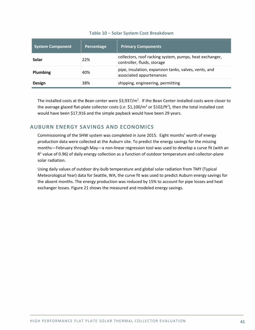
HIGH PE RFORMANCE FLAT PLATE SOLAR THE RMAL COLLE CTOR E VALUATION 41
Table 10 – Solar System Cost Breakdown
System Component Percentage Primary Components
Solar 22% collectors, roof racking system, pumps, heat exchanger, controller, fluids, storage
Plumbing 40% pipe, insulation, expansion tanks, valves, vents, and associated appurtenances
Design 38% shipping, engineering, permitting
The installed costs at the Bean center were $3,937/m2. If the Bean Center installed costs were closer to the average glazed flat-plate collector costs (i.e. $1,100/m2 or $102/ft2), then the total installed cost would have been $17,916 and the simple payback would have been 29 years.
AUBURN ENERGY SAVINGS AND ECONOMICS Commissioning of the SHW system was completed in June 2015. Eight months’ worth of energy production data were collected at the Auburn site. To predict the energy savings for the missing months—February through May—a non-linear regression tool was used to develop a curve fit (with an R2 value of 0.96) of daily energy collection as a function of outdoor temperature and collector-plane solar radiation.
Using daily values of outdoor dry-bulb temperature and global solar radiation from TMY (Typical Meteorological Year) data for Seattle, WA, the curve fit was used to predict Auburn energy savings for the absent months. The energy production was reduced by 15% to account for pipe losses and heat exchanger losses. Figure 21 shows the measured and modeled energy savings.
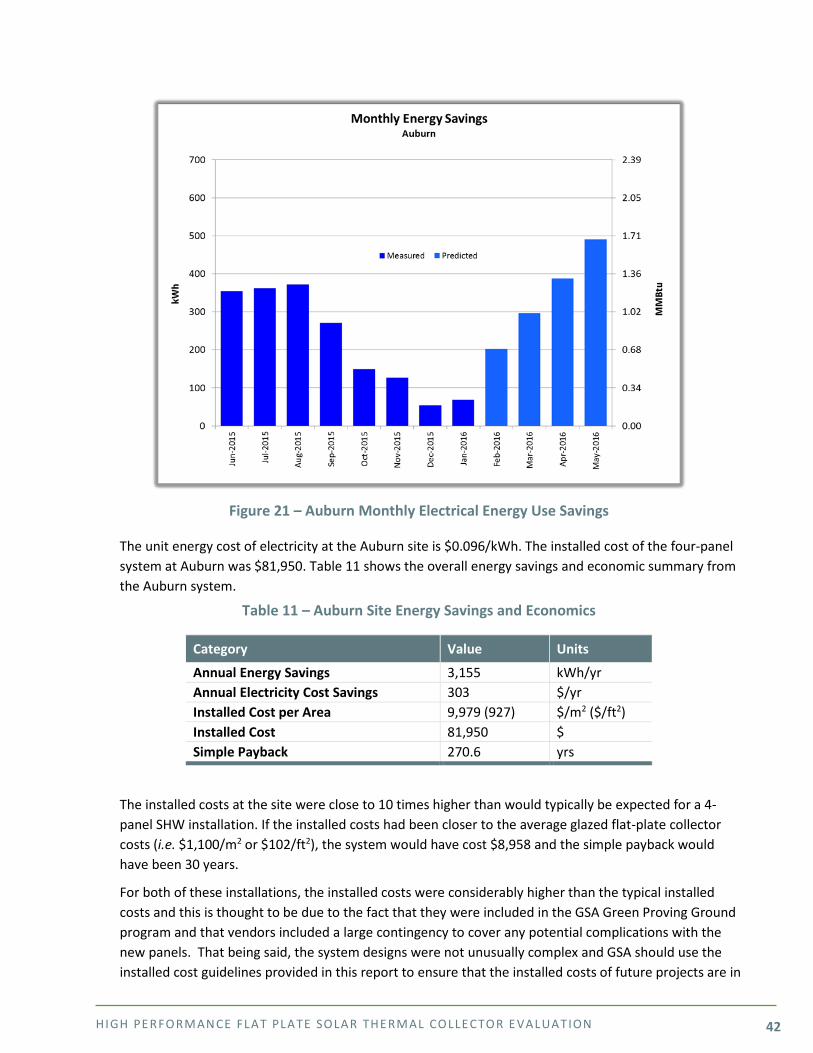
HIGH PE RFORMANCE FLAT PLATE SOLAR THE RMAL COLLE CTOR E VALUATION 42
Figure 21 – Auburn Monthly Electrical Energy Use Savings
The unit energy cost of electricity at the Auburn site is $0.096/kWh. The installed cost of the four-panel system at Auburn was $81,950. Table 11 shows the overall energy savings and economic summary from the Auburn system.
Table 11 – Auburn Site Energy Savings and Economics
Category Value Units
Annual Energy Savings 3,155 kWh/yr Annual Electricity Cost Savings 303 $/yr Installed Cost per Area 9,979 (927) $/m2 ($/ft2) Installed Cost 81,950 $ Simple Payback 270.6 yrs
The installed costs at the site were close to 10 times higher than would typically be expected for a 4-panel SHW installation. If the installed costs had been closer to the average glazed flat-plate collector costs (i.e. $1,100/m2 or $102/ft2), the system would have cost $8,958 and the simple payback would have been 30 years.
For both of these installations, the installed costs were considerably higher than the typical installed costs and this is thought to be due to the fact that they were included in the GSA Green Proving Ground program and that vendors included a large contingency to cover any potential complications with the new panels. That being said, the system designs were not unusually complex and GSA should use the installed cost guidelines provided in this report to ensure that the installed costs of future projects are in
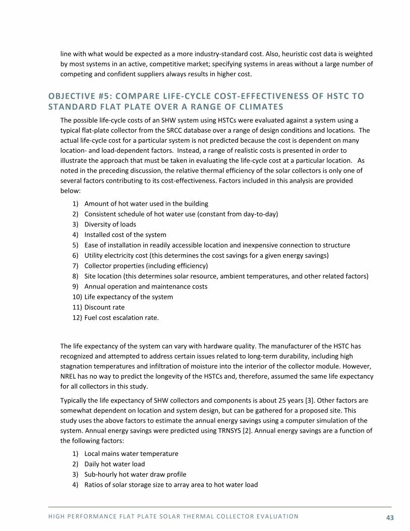
HIGH PE RFORMANCE FLAT PLATE SOLAR THE RMAL COLLE CTOR E VALUATION 43
line with what would be expected as a more industry-standard cost. Also, heuristic cost data is weighted by most systems in an active, competitive market; specifying systems in areas without a large number of competing and confident suppliers always results in higher cost.
OBJECTIVE #5: COMPARE LIFE-CYCLE COST-EFFECTIVENESS OF HSTC TO STANDARD FLAT PLATE OVER A RANGE OF CLIMATES
The possible life-cycle costs of an SHW system using HSTCs were evaluated against a system using a typical flat-plate collector from the SRCC database over a range of design conditions and locations. The actual life-cycle cost for a particular system is not predicted because the cost is dependent on many location- and load-dependent factors. Instead, a range of realistic costs is presented in order to illustrate the approach that must be taken in evaluating the life-cycle cost at a particular location. As noted in the preceding discussion, the relative thermal efficiency of the solar collectors is only one of several factors contributing to its cost-effectiveness. Factors included in this analysis are provided below:
1) Amount of hot water used in the building 2) Consistent schedule of hot water use (constant from day-to-day) 3) Diversity of loads 4) Installed cost of the system 5) Ease of installation in readily accessible location and inexpensive connection to structure 6) Utility electricity cost (this determines the cost savings for a given energy savings) 7) Collector properties (including efficiency) 8) Site location (this determines solar resource, ambient temperatures, and other related factors) 9) Annual operation and maintenance costs 10) Life expectancy of the system 11) Discount rate 12) Fuel cost escalation rate.
The life expectancy of the system can vary with hardware quality. The manufacturer of the HSTC has recognized and attempted to address certain issues related to long-term durability, including high stagnation temperatures and infiltration of moisture into the interior of the collector module. However, NREL has no way to predict the longevity of the HSTCs and, therefore, assumed the same life expectancy for all collectors in this study.
Typically the life expectancy of SHW collectors and components is about 25 years [3]. Other factors are somewhat dependent on location and system design, but can be gathered for a proposed site. This study uses the above factors to estimate the annual energy savings using a computer simulation of the system. Annual energy savings were predicted using TRNSYS [2]. Annual energy savings are a function of the following factors:
1) Local mains water temperature 2) Daily hot water load 3) Sub-hourly hot water draw profile 4) Ratios of solar storage size to array area to hot water load
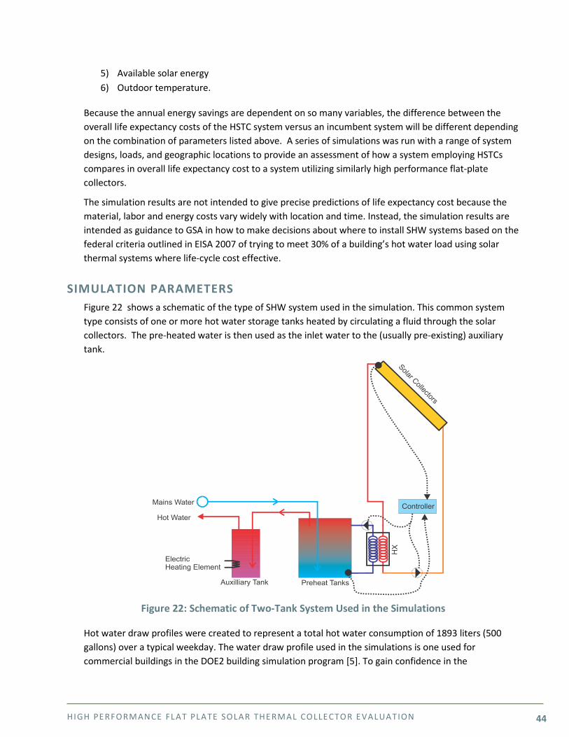
HIGH PE RFORMANCE FLAT PLATE SOLAR THE RMAL COLLE CTOR E VALUATION 44
5) Available solar energy 6) Outdoor temperature.
Because the annual energy savings are dependent on so many variables, the difference between the overall life expectancy costs of the HSTC system versus an incumbent system will be different depending on the combination of parameters listed above. A series of simulations was run with a range of system designs, loads, and geographic locations to provide an assessment of how a system employing HSTCs compares in overall life expectancy cost to a system utilizing similarly high performance flat-plate collectors.
The simulation results are not intended to give precise predictions of life expectancy cost because the material, labor and energy costs vary widely with location and time. Instead, the simulation results are intended as guidance to GSA in how to make decisions about where to install SHW systems based on the federal criteria outlined in EISA 2007 of trying to meet 30% of a building’s hot water load using solar thermal systems where life-cycle cost effective.
SIMULATION PARAMETERS Figure 22 shows a schematic of the type of SHW system used in the simulation. This common system type consists of one or more hot water storage tanks heated by circulating a fluid through the solar collectors. The pre-heated water is then used as the inlet water to the (usually pre-existing) auxiliary tank.
Figure 22: Schematic of Two-Tank System Used in the Simulations
Hot water draw profiles were created to represent a total hot water consumption of 1893 liters (500 gallons) over a typical weekday. The water draw profile used in the simulations is one used for commercial buildings in the DOE2 building simulation program [5]. To gain confidence in the
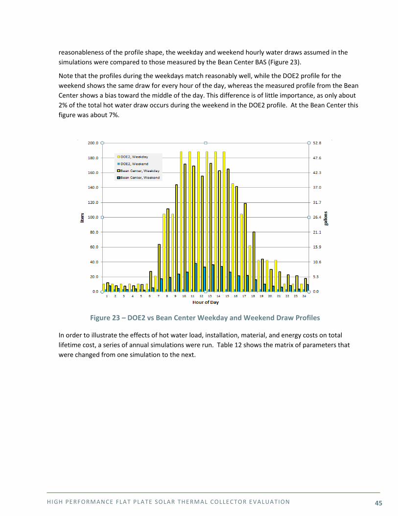
HIGH PE RFORMANCE FLAT PLATE SOLAR THE RMAL COLLE CTOR E VALUATION 45
reasonableness of the profile shape, the weekday and weekend hourly water draws assumed in the simulations were compared to those measured by the Bean Center BAS (Figure 23).
Note that the profiles during the weekdays match reasonably well, while the DOE2 profile for the weekend shows the same draw for every hour of the day, whereas the measured profile from the Bean Center shows a bias toward the middle of the day. This difference is of little importance, as only about 2% of the total hot water draw occurs during the weekend in the DOE2 profile. At the Bean Center this figure was about 7%.
Figure 23 – DOE2 vs Bean Center Weekday and Weekend Draw Profiles
In order to illustrate the effects of hot water load, installation, material, and energy costs on total lifetime cost, a series of annual simulations were run. Table 12 shows the matrix of parameters that were changed from one simulation to the next.
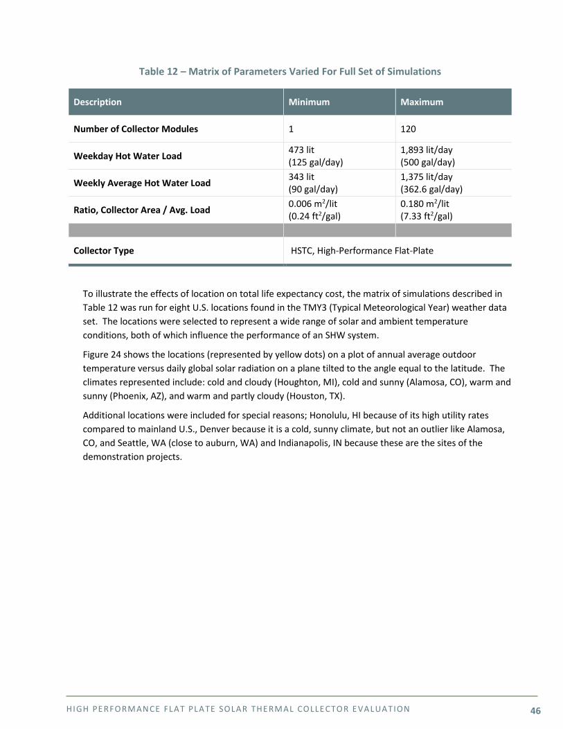
HIGH PE RFORMANCE FLAT PLATE SOLAR THE RMAL COLLE CTOR E VALUATION 46
Table 12 – Matrix of Parameters Varied For Full Set of Simulations
Description Minimum Maximum
Number of Collector Modules 1 120
Weekday Hot Water Load 473 lit (125 gal/day)
1,893 lit/day (500 gal/day)
Weekly Average Hot Water Load 343 lit (90 gal/day)
1,375 lit/day (362.6 gal/day)
Ratio, Collector Area / Avg. Load 0.006 m2/lit (0.24 ft2/gal)
0.180 m2/lit (7.33 ft2/gal)
Collector Type HSTC, High-Performance Flat-Plate
To illustrate the effects of location on total life expectancy cost, the matrix of simulations described in Table 12 was run for eight U.S. locations found in the TMY3 (Typical Meteorological Year) weather data set. The locations were selected to represent a wide range of solar and ambient temperature conditions, both of which influence the performance of an SHW system.
Figure 24 shows the locations (represented by yellow dots) on a plot of annual average outdoor temperature versus daily global solar radiation on a plane tilted to the angle equal to the latitude. The climates represented include: cold and cloudy (Houghton, MI), cold and sunny (Alamosa, CO), warm and sunny (Phoenix, AZ), and warm and partly cloudy (Houston, TX).
Additional locations were included for special reasons; Honolulu, HI because of its high utility rates compared to mainland U.S., Denver because it is a cold, sunny climate, but not an outlier like Alamosa, CO, and Seattle, WA (close to auburn, WA) and Indianapolis, IN because these are the sites of the demonstration projects.
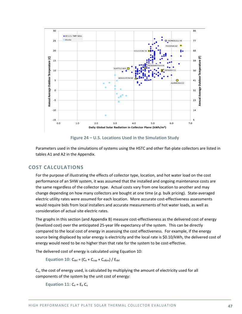
HIGH PE RFORMANCE FLAT PLATE SOLAR THE RMAL COLLE CTOR E VALUATION 47
Figure 24 – U.S. Locations Used in the Simulation Study
Parameters used in the simulations of systems using the HSTC and other flat-plate collectors are listed in tables A1 and A2 in the Appendix.
COST CALCULATIONS For the purpose of illustrating the effects of collector type, location, and hot water load on the cost performance of an SHW system, it was assumed that the installed and ongoing maintenance costs are the same regardless of the collector type. Actual costs vary from one location to another and may change depending on how many collectors are bought at one time (e.g. bulk pricing). State-averaged electric utility rates were assumed for each location. More accurate cost-effectiveness assessments would require bids from local installers and accurate measurements of hot water loads, as well as consideration of actual site electric rates.
The graphs in this section (and Appendix B) measure cost-effectiveness as the delivered cost of energy (levelized cost) over the anticipated 25-year life expectancy of the system. This can be directly compared to the local cost of energy in assessing the cost effectiveness. For example, if the energy source being displaced by solar energy is electricity and the local rate is $0.10/kWh, the delivered cost of energy would need to be no higher than that rate for the system to be cost-effective.
The delivered cost of energy is calculated using Equation 10:
Equation 10: Cdel = (Ce + Ccap + Co&m) / Edel
Ce, the cost of energy used, is calculated by multiplying the amount of electricity used for all components of the system by the unit cost of energy:
Equation 11: Ce = Ee Cu
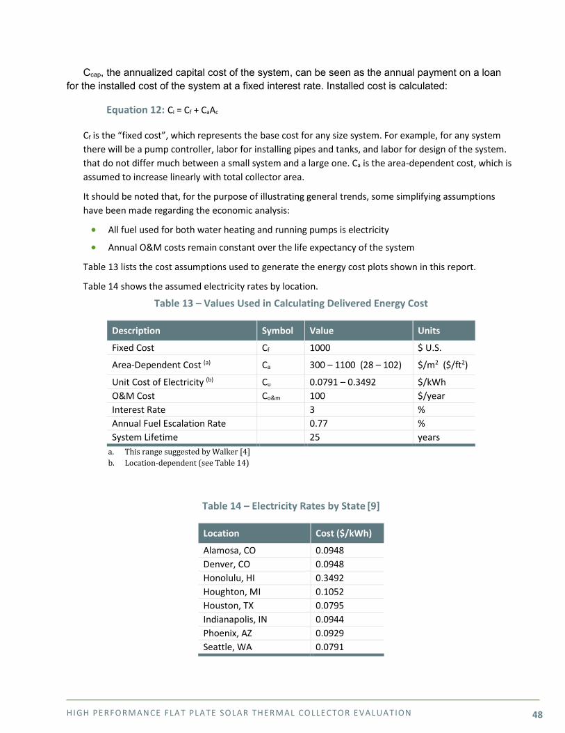
HIGH PE RFORMANCE FLAT PLATE SOLAR THE RMAL COLLE CTOR E VALUATION 48
Ccap, the annualized capital cost of the system, can be seen as the annual payment on a loan for the installed cost of the system at a fixed interest rate. Installed cost is calculated:
Equation 12: Ci = Cf + CaAc
Cf is the “fixed cost”, which represents the base cost for any size system. For example, for any system there will be a pump controller, labor for installing pipes and tanks, and labor for design of the system. that do not differ much between a small system and a large one. Ca is the area-dependent cost, which is assumed to increase linearly with total collector area.
It should be noted that, for the purpose of illustrating general trends, some simplifying assumptions have been made regarding the economic analysis:
• All fuel used for both water heating and running pumps is electricity
• Annual O&M costs remain constant over the life expectancy of the system
Table 13 lists the cost assumptions used to generate the energy cost plots shown in this report.
Table 14 shows the assumed electricity rates by location.
Table 13 – Values Used in Calculating Delivered Energy Cost
Description Symbol Value Units
Fixed Cost Cf 1000 $ U.S.
Area-Dependent Cost (a) Ca 300 – 1100 (28 – 102) $/m2 ($/ft2)
Unit Cost of Electricity (b) Cu 0.0791 – 0.3492 $/kWh O&M Cost Co&m 100 $/year Interest Rate 3 % Annual Fuel Escalation Rate 0.77 % System Lifetime 25 years
a. This range suggested by Walker [4] b. Location-dependent (see Table 14)
Table 14 – Electricity Rates by State [9]
Location Cost ($/kWh)
Alamosa, CO 0.0948 Denver, CO 0.0948 Honolulu, HI 0.3492 Houghton, MI 0.1052 Houston, TX 0.0795 Indianapolis, IN 0.0944 Phoenix, AZ 0.0929 Seattle, WA 0.0791
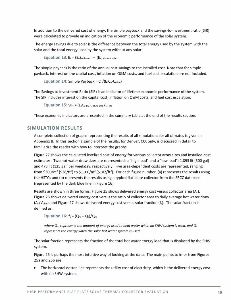
HIGH PE RFORMANCE FLAT PLATE SOLAR THE RMAL COLLE CTOR E VALUATION 49
In addition to the delivered cost of energy, the simple payback and the savings-to-investment ratio (SIR) were calculated to provide an indication of the economic performance of the solar system.
The energy savings due to solar is the difference between the total energy used by the system with the solar and the total energy used by the system without any solar:
Equation 13: Es = (Ee)with solar – (Ee)without solar
The simple payback is the ratio of the annual cost savings to the installed cost. Note that for simple payback, interest on the capital cost, inflation on O&M costs, and fuel cost escalation are not included.
Equation 14: Simple Payback = Ci /(EsCu-Co&m)
The Savings to Investment Ratio (SIR) is an indicator of lifetime economic performance of the system. The SIR includes interest on the capital cost, inflation on O&M costs, and fuel cost escalation:
Equation 15: SIR = (EsCu-life-Co&m-life) /Ci-life
These economic indicators are presented in the summary table at the end of the results section.
SIMULATION RESULTS A complete collection of graphs representing the results of all simulations for all climates is given in Appendix B. In this section a sample of the results, for Denver, CO, only, is discussed in detail to familiarize the reader with how to interpret the graphs.
Figure 27 shows the calculated levelized cost of energy for various collector array sizes and installed-cost estimates. Two hot water draw sizes are represented: a “high load” and a “low load”: 1,893 lit (500 gal) and 473 lit (125 gal) per weekday, respectively. Five area-dependent costs are represented, ranging from $300/m2 ($28/ft2) to $1100/m2 ($102/ft2). For each figure number, (a) represents the results using the HSTCs and (b) represents the results using a typical flat-plate collector from the SRCC database (represented by the dark blue line in Figure 16).
Results are shown in three forms: Figure 25 shows delivered energy cost versus collector area (Ac), Figure 26 shows delivered energy cost versus the ratio of collector area to daily average hot water draw (Ac/Vdhw), and Figure 27 shows delivered energy cost versus solar fraction (fs). The solar fraction is defined as:
Equation 16: fs = (Qns – Qs)/Qns
where Qns represents the amount of energy used to heat water when no SHW system is used, and Qs represents the energy when the solar hot water system is used.
The solar fraction represents the fraction of the total hot water energy load that is displaced by the SHW system.
Figure 25 is perhaps the most intuitive way of looking at the data. The main points to infer from Figures 25a and 25b are:
• The horizontal dotted line represents the utility cost of electricity, which is the delivered energy cost with no SHW system.
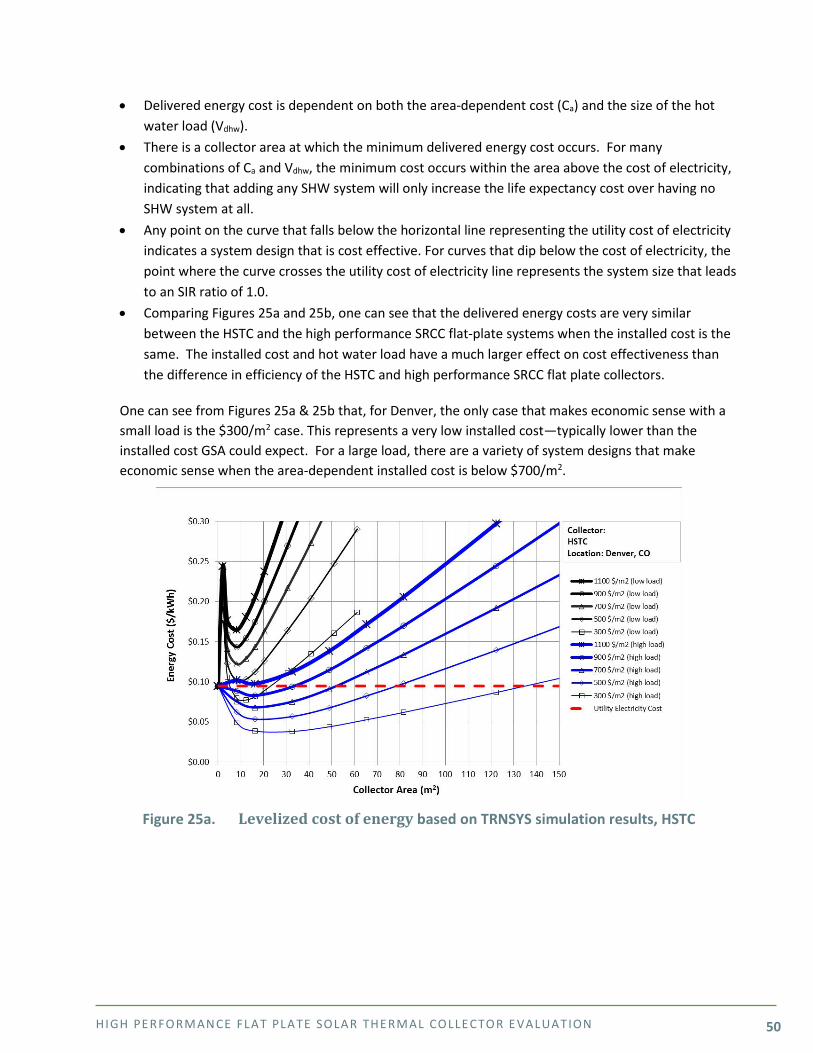
HIGH PE RFORMANCE FLAT PLATE SOLAR THE RMAL COLLE CTOR E VALUATION 50
• Delivered energy cost is dependent on both the area-dependent cost (Ca) and the size of the hot water load (Vdhw).
• There is a collector area at which the minimum delivered energy cost occurs. For many combinations of Ca and Vdhw, the minimum cost occurs within the area above the cost of electricity, indicating that adding any SHW system will only increase the life expectancy cost over having no SHW system at all.
• Any point on the curve that falls below the horizontal line representing the utility cost of electricity indicates a system design that is cost effective. For curves that dip below the cost of electricity, the point where the curve crosses the utility cost of electricity line represents the system size that leads to an SIR ratio of 1.0.
• Comparing Figures 25a and 25b, one can see that the delivered energy costs are very similar between the HSTC and the high performance SRCC flat-plate systems when the installed cost is the same. The installed cost and hot water load have a much larger effect on cost effectiveness than the difference in efficiency of the HSTC and high performance SRCC flat plate collectors.
One can see from Figures 25a & 25b that, for Denver, the only case that makes economic sense with a small load is the $300/m2 case. This represents a very low installed cost—typically lower than the installed cost GSA could expect. For a large load, there are a variety of system designs that make economic sense when the area-dependent installed cost is below $700/m2.
Figure 25a. Levelized cost of energy based on TRNSYS simulation results, HSTC
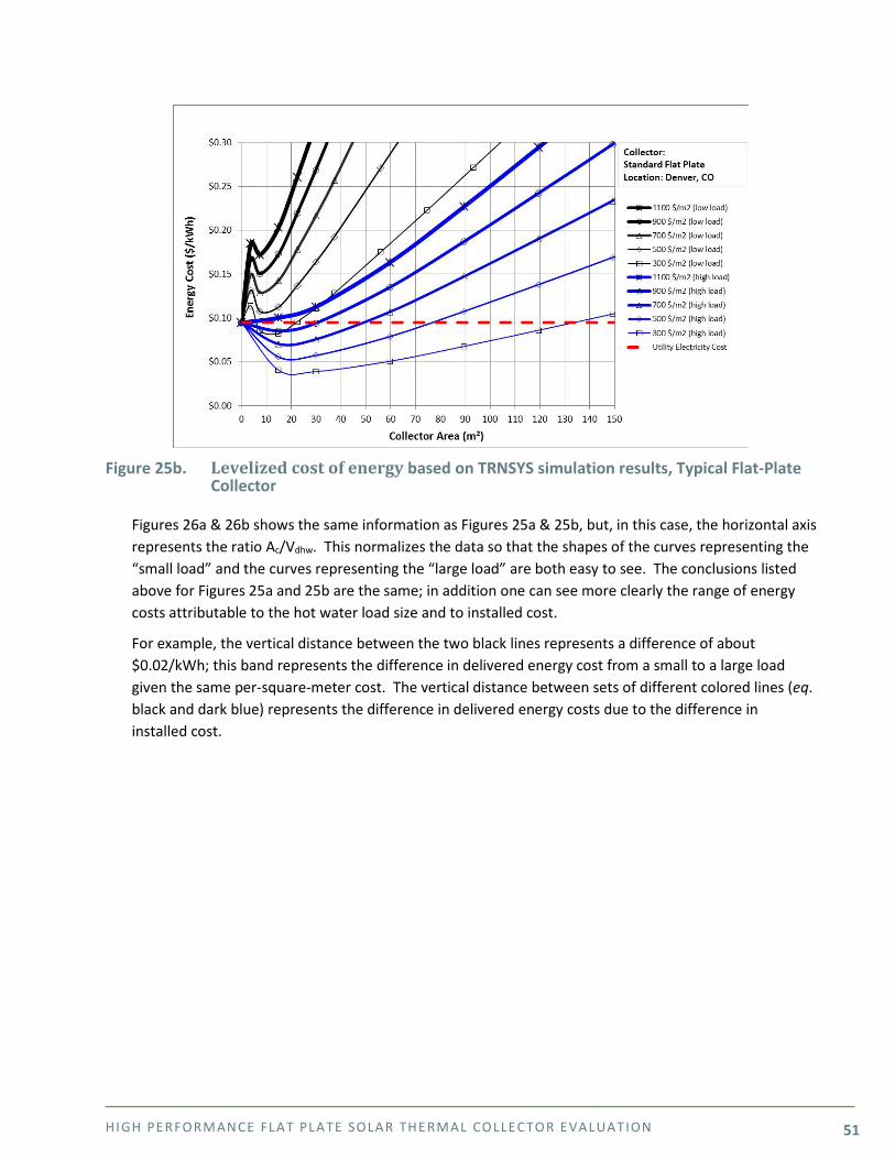
HIGH PE RFORMANCE FLAT PLATE SOLAR THE RMAL COLLE CTOR E VALUATION 51
Figure 25b. Levelized cost of energy based on TRNSYS simulation results, Typical Flat-Plate
Collector
Figures 26a & 26b shows the same information as Figures 25a & 25b, but, in this case, the horizontal axis represents the ratio Ac/Vdhw. This normalizes the data so that the shapes of the curves representing the “small load” and the curves representing the “large load” are both easy to see. The conclusions listed above for Figures 25a and 25b are the same; in addition one can see more clearly the range of energy costs attributable to the hot water load size and to installed cost.
For example, the vertical distance between the two black lines represents a difference of about $0.02/kWh; this band represents the difference in delivered energy cost from a small to a large load given the same per-square-meter cost. The vertical distance between sets of different colored lines (eq. black and dark blue) represents the difference in delivered energy costs due to the difference in installed cost.
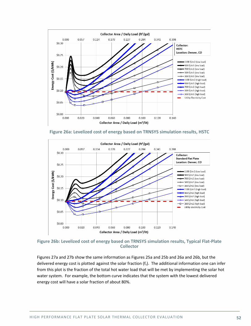
HIGH PE RFORMANCE FLAT PLATE SOLAR THE RMAL COLLE CTOR E VALUATION 52
Figure 26a: Levelized cost of energy based on TRNSYS simulation results, HSTC
Figure 26b: Levelized cost of energy based on TRNSYS simulation results, Typical Flat-Plate
Collector
Figures 27a and 27b show the same information as Figures 25a and 25b and 26a and 26b, but the delivered energy cost is plotted against the solar fraction (fs). The additional information one can infer from this plot is the fraction of the total hot water load that will be met by implementing the solar hot water system. For example, the bottom curve indicates that the system with the lowest delivered energy cost will have a solar fraction of about 80%.
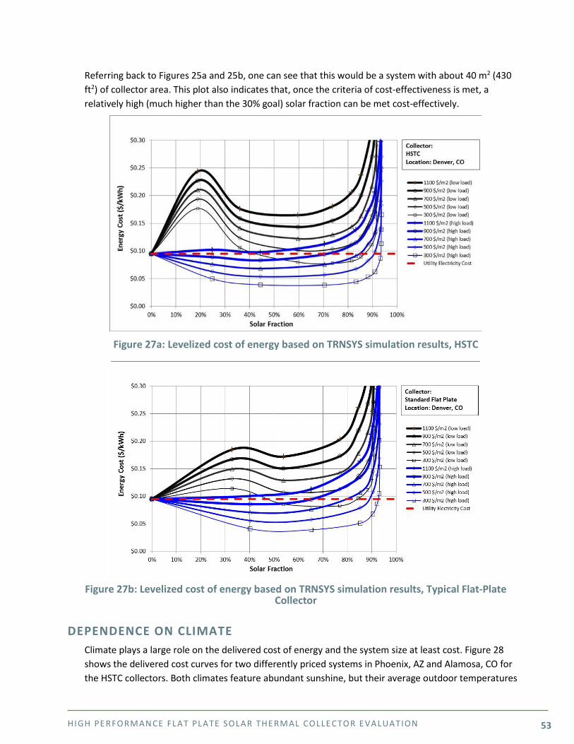
HIGH PE RFORMANCE FLAT PLATE SOLAR THE RMAL COLLE CTOR E VALUATION 53
Referring back to Figures 25a and 25b, one can see that this would be a system with about 40 m2 (430 ft2) of collector area. This plot also indicates that, once the criteria of cost-effectiveness is met, a relatively high (much higher than the 30% goal) solar fraction can be met cost-effectively.
Figure 27a: Levelized cost of energy based on TRNSYS simulation results, HSTC
Figure 27b: Levelized cost of energy based on TRNSYS simulation results, Typical Flat-Plate
Collector
DEPENDENCE ON CLIMATE Climate plays a large role on the delivered cost of energy and the system size at least cost. Figure 28 shows the delivered cost curves for two differently priced systems in Phoenix, AZ and Alamosa, CO for the HSTC collectors. Both climates feature abundant sunshine, but their average outdoor temperatures
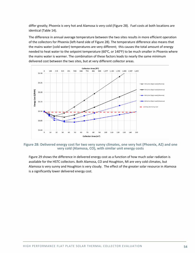
HIGH PE RFORMANCE FLAT PLATE SOLAR THE RMAL COLLE CTOR E VALUATION 54
differ greatly; Phoenix is very hot and Alamosa is very cold (Figure 28). Fuel costs at both locations are identical (Table 14).
The difference in annual average temperature between the two sites results in more efficient operation of the collectors for Phoenix (left-hand side of Figure 28). The temperature difference also means that the mains water (cold water) temperatures are very different; this causes the total amount of energy needed to heat water to the setpoint temperature (60oC, or 140oF) to be much smaller in Phoenix where the mains water is warmer. The combination of these factors leads to nearly the same minimum delivered cost between the two sites, but at very different collector areas.
Figure 28: Delivered energy cost for two very sunny climates, one very hot (Phoenix, AZ) and one
very cold (Alamosa, CO), with similar unit energy costs
Figure 29 shows the difference in delivered energy cost as a function of how much solar radiation is available for the HSTC collectors. Both Alamosa, CO and Houghton, MI are very cold climates, but Alamosa is very sunny and Houghton is very cloudy. The effect of the greater solar resource in Alamosa is a significantly lower delivered energy cost.
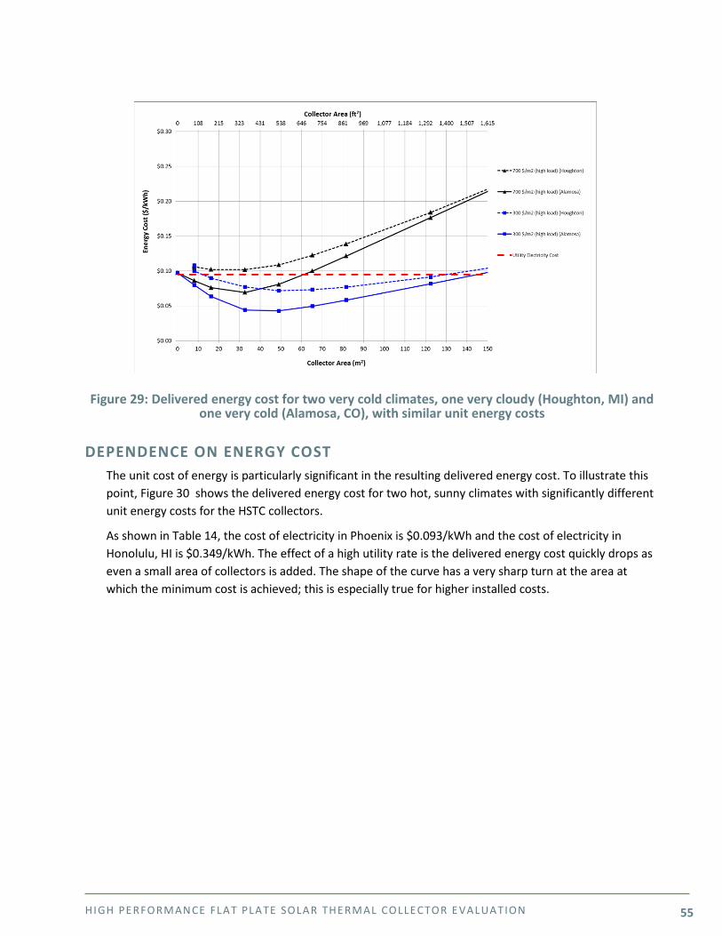
HIGH PE RFORMANCE FLAT PLATE SOLAR THE RMAL COLLE CTOR E VALUATION 55
Figure 29: Delivered energy cost for two very cold climates, one very cloudy (Houghton, MI) and
one very cold (Alamosa, CO), with similar unit energy costs
DEPENDENCE ON ENERGY COST The unit cost of energy is particularly significant in the resulting delivered energy cost. To illustrate this point, Figure 30 shows the delivered energy cost for two hot, sunny climates with significantly different unit energy costs for the HSTC collectors.
As shown in Table 14, the cost of electricity in Phoenix is $0.093/kWh and the cost of electricity in Honolulu, HI is $0.349/kWh. The effect of a high utility rate is the delivered energy cost quickly drops as even a small area of collectors is added. The shape of the curve has a very sharp turn at the area at which the minimum cost is achieved; this is especially true for higher installed costs.
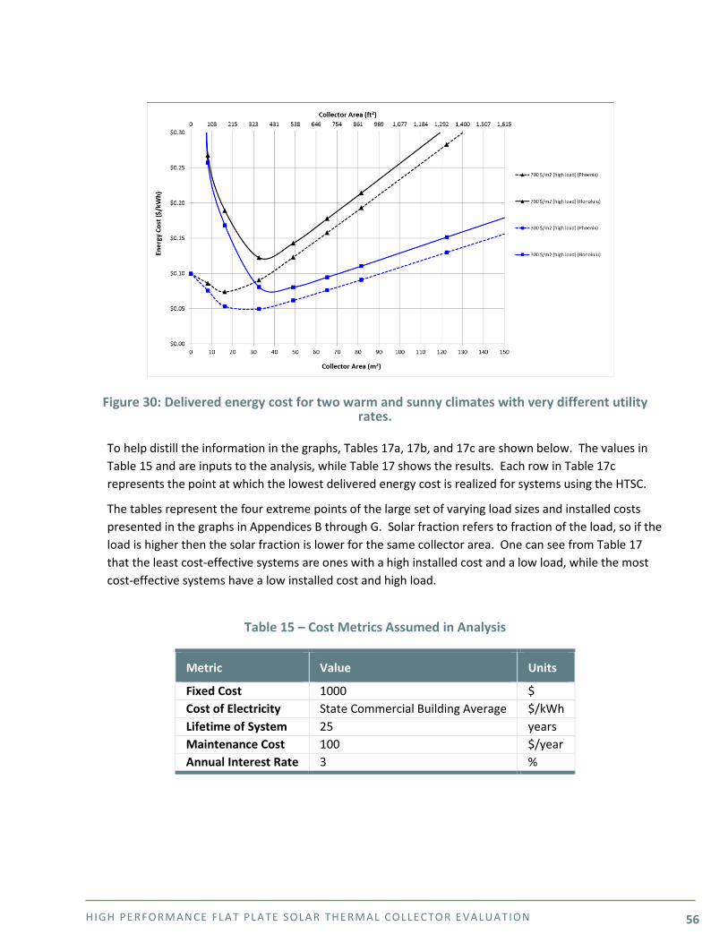
HIGH PE RFORMANCE FLAT PLATE SOLAR THE RMAL COLLE CTOR E VALUATION 56
Figure 30: Delivered energy cost for two warm and sunny climates with very different utility
rates.
To help distill the information in the graphs, Tables 17a, 17b, and 17c are shown below. The values in Table 15 and are inputs to the analysis, while Table 17 shows the results. Each row in Table 17c represents the point at which the lowest delivered energy cost is realized for systems using the HTSC.
The tables represent the four extreme points of the large set of varying load sizes and installed costs presented in the graphs in Appendices B through G. Solar fraction refers to fraction of the load, so if the load is higher then the solar fraction is lower for the same collector area. One can see from Table 17 that the least cost-effective systems are ones with a high installed cost and a low load, while the most cost-effective systems have a low installed cost and high load.
Table 15 – Cost Metrics Assumed in Analysis
Metric Value Units
Fixed Cost 1000 $ Cost of Electricity State Commercial Building Average $/kWh Lifetime of System 25 years Maintenance Cost 100 $/year Annual Interest Rate 3 %
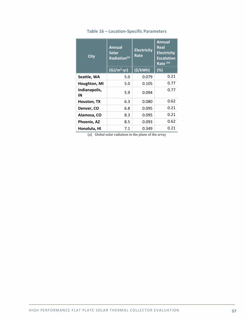
HIGH PE RFORMANCE FLAT PLATE SOLAR THE RMAL COLLE CTOR E VALUATION 57
Table 16 – Location-Specific Parameters
City
Annual Solar Radiation(a)
Electricity Rate
Annual Real Electricity Escalation Rate (iv)
(GJ/m2-yr) ($/kWh) (%) Seattle, WA 5.0 0.079 0.21
Houghton, MI 5.0 0.105 0.77 Indianapolis, IN 5.9 0.094 0.77
Houston, TX 6.3 0.080 0.62
Denver, CO 6.8 0.095 0.21
Alamosa, CO 8.3 0.095 0.21
Phoenix, AZ 8.5 0.093 0.62
Honolulu, HI 7.1 0.349 0.21 (a) Global solar radiation in the plane of the array
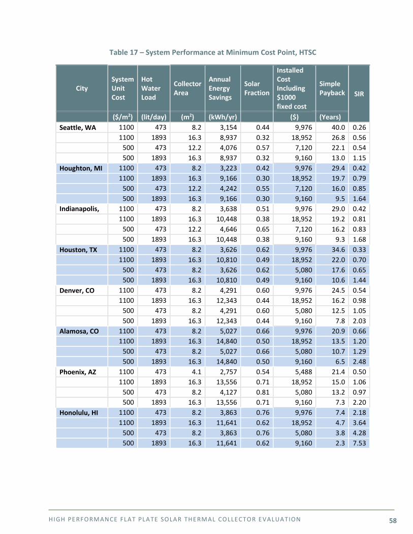
HIGH PE RFORMANCE FLAT PLATE SOLAR THE RMAL COLLE CTOR E VALUATION 58
Table 17 – System Performance at Minimum Cost Point, HTSC
City System Unit Cost
Hot Water Load
Collector Area
Annual Energy Savings
Solar Fraction
Installed Cost Including $1000 fixed cost
Simple Payback SIR
($/m2) (lit/day) (m2) (kWh/yr) ($) (Years) Seattle, WA 1100 473 8.2 3,154 0.44 9,976 40.0 0.26 1100 1893 16.3 8,937 0.32 18,952 26.8 0.56 500 473 12.2 4,076 0.57 7,120 22.1 0.54 500 1893 16.3 8,937 0.32 9,160 13.0 1.15 Houghton, MI 1100 473 8.2 3,223 0.42 9,976 29.4 0.42 1100 1893 16.3 9,166 0.30 18,952 19.7 0.79 500 473 12.2 4,242 0.55 7,120 16.0 0.85 500 1893 16.3 9,166 0.30 9,160 9.5 1.64 Indianapolis,
1100 473 8.2 3,638 0.51 9,976 29.0 0.42
1100 1893 16.3 10,448 0.38 18,952 19.2 0.81 500 473 12.2 4,646 0.65 7,120 16.2 0.83 500 1893 16.3 10,448 0.38 9,160 9.3 1.68 Houston, TX 1100 473 8.2 3,626 0.62 9,976 34.6 0.33 1100 1893 16.3 10,810 0.49 18,952 22.0 0.70 500 473 8.2 3,626 0.62 5,080 17.6 0.65 500 1893 16.3 10,810 0.49 9,160 10.6 1.44 Denver, CO 1100 473 8.2 4,291 0.60 9,976 24.5 0.54 1100 1893 16.3 12,343 0.44 18,952 16.2 0.98 500 473 8.2 4,291 0.60 5,080 12.5 1.05 500 1893 16.3 12,343 0.44 9,160 7.8 2.03 Alamosa, CO 1100 473 8.2 5,027 0.66 9,976 20.9 0.66 1100 1893 16.3 14,840 0.50 18,952 13.5 1.20 500 473 8.2 5,027 0.66 5,080 10.7 1.29 500 1893 16.3 14,840 0.50 9,160 6.5 2.48 Phoenix, AZ 1100 473 4.1 2,757 0.54 5,488 21.4 0.50 1100 1893 16.3 13,556 0.71 18,952 15.0 1.06 500 473 8.2 4,127 0.81 5,080 13.2 0.97 500 1893 16.3 13,556 0.71 9,160 7.3 2.20 Honolulu, HI 1100 473 8.2 3,863 0.76 9,976 7.4 2.18 1100 1893 16.3 11,641 0.62 18,952 4.7 3.64 500 473 8.2 3,863 0.76 5,080 3.8 4.28 500 1893 16.3 11,641 0.62 9,160 2.3 7.53
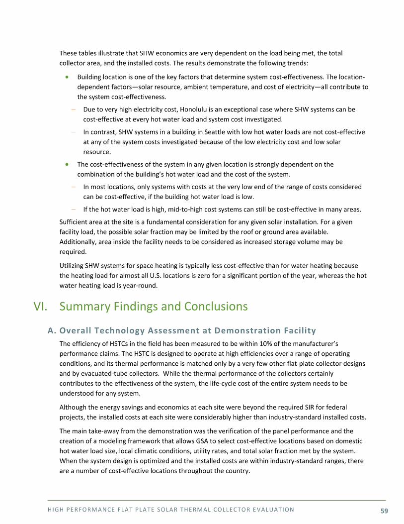
HIGH PE RFORMANCE FLAT PLATE SOLAR THE RMAL COLLE CTOR E VALUATION 59
These tables illustrate that SHW economics are very dependent on the load being met, the total collector area, and the installed costs. The results demonstrate the following trends:
• Building location is one of the key factors that determine system cost-effectiveness. The location-dependent factors—solar resource, ambient temperature, and cost of electricity—all contribute to the system cost-effectiveness.
− Due to very high electricity cost, Honolulu is an exceptional case where SHW systems can be cost-effective at every hot water load and system cost investigated.
− In contrast, SHW systems in a building in Seattle with low hot water loads are not cost-effective at any of the system costs investigated because of the low electricity cost and low solar resource.
• The cost-effectiveness of the system in any given location is strongly dependent on the combination of the building’s hot water load and the cost of the system.
− In most locations, only systems with costs at the very low end of the range of costs considered can be cost-effective, if the building hot water load is low.
− If the hot water load is high, mid-to-high cost systems can still be cost-effective in many areas.
Sufficient area at the site is a fundamental consideration for any given solar installation. For a given facility load, the possible solar fraction may be limited by the roof or ground area available. Additionally, area inside the facility needs to be considered as increased storage volume may be required.
Utilizing SHW systems for space heating is typically less cost-effective than for water heating because the heating load for almost all U.S. locations is zero for a significant portion of the year, whereas the hot water heating load is year-round.
VI. Summary Findings and Conclusions
A. Overall Technology Assessment at Demonstration Facility The efficiency of HSTCs in the field has been measured to be within 10% of the manufacturer’s performance claims. The HSTC is designed to operate at high efficiencies over a range of operating conditions, and its thermal performance is matched only by a very few other flat-plate collector designs and by evacuated-tube collectors. While the thermal performance of the collectors certainly contributes to the effectiveness of the system, the life-cycle cost of the entire system needs to be understood for any system.
Although the energy savings and economics at each site were beyond the required SIR for federal projects, the installed costs at each site were considerably higher than industry-standard installed costs.
The main take-away from the demonstration was the verification of the panel performance and the creation of a modeling framework that allows GSA to select cost-effective locations based on domestic hot water load size, local climatic conditions, utility rates, and total solar fraction met by the system. When the system design is optimized and the installed costs are within industry-standard ranges, there are a number of cost-effective locations throughout the country.
HIGH PE RFORMANCE FLAT PLATE SOLAR THE RMAL COLLE CTOR E VALUATION 60
B. Best Practice There are a number of general best practice areas and lessons learned that can be taken away from the demonstration:
• Roof Availability – Facilities with roofs that won’t need to be replaced for 20 to 25 years and with sufficient availability to accommodate an SHW system should be targeted. Ease of structural attachment without expensive members to carry loads to structure.
• Implement Efficiency First – The existing DHW equipment should be analyzed prior to the installation of an SHW system. All applicable water conservation and energy efficiency opportunities should be implemented before sizing a solar thermal system.
• Central Hot Water Systems – Facilities with centralized DHW systems should be targeted for SHW installations due to economy of scale and diversity of loads, and the baseline DHW load should be metered before designing a solar thermal system to size the system properly. Facilities with small decentralized point of use DHW systems are not appropriate for solar thermal installations.
• Large, Consistent Hot Water Loads – As shown, the larger the load being offset, the more cost-effective the system. Although specific requirements cannot be provided, a system with a 1,893 liter (500 gallon) per weekday load showed considerably better economics than a system with a 473 liter (125 gallon) per weekday load. The size of the building does not necessarily translate to hot water load. In large buildings, such as the Bean Center, there are many hot water loads (e.g. cafeteria and bathrooms) served by many separate systems. A building manager will have an idea about what hot water loads are being served by which systems in the building. Higher hot water loads are expected in facilities with kitchens, heated pools, and shower facilities. GSA facilities with these larger loads should be targeted.
• High Energy Costs – The natural gas industry has experienced significant cost reductions over the last few years. The economics of the solar thermal system is sensitive to fuel source costs; the unit cost of electricity ($/kWh) is seven times higher than natural gas in certain locations. Locations with electric resistance domestic hot water heaters and high electric rates should be targeted.
• Use Accurate System Design Tools to Calculate Life-Cycle Costs and Optimize Cost Effectiveness– An approach to determining the correct system design to meet a particular cost-effectiveness objective has been demonstrated in this report. It is suggested that this approach be followed when evaluating whether or not to install a SHW system at a particular facility. A detailed sub-hourly simulation program should be used and the system should be modeled accurately with SRCC-rated solar thermal panel performance data. This will aid in determining the correct sizing of the system and enable a more accurate economic analysis.
• Collector Efficiency – The demonstration showed that HSTCs are some of the most efficient collectors on the market for higher-fluid-temperature applications such as industrial process heat, space heating, and hot water hydronic loop re-heating, but show only moderate performance improvement, for some climates, for standard domestic hot water applications where ground-temperature water is heated to a setpoint. However, collector efficiency is only one part of a large number of factors that influence the overall life-cycle cost of the SHW system. In some instances a less-efficient but less-expensive collector may be the more wise choice. When the cost-effectiveness of the SHW system is the ultimate metric upon which decisions are to be made,
HIGH PE RFORMANCE FLAT PLATE SOLAR THE RMAL COLLE CTOR E VALUATION 61
the choice of what collector to use should be based on the procedure outlined in this report, which takes into account the performance and costs of all parts of the SHW system.
• Trained System Installers – It is important that the designers and installers of a solar hot water system have sufficient training and experience with solar hot water systems. Although in principle the components of a SHW system are similar to other common plumbing components, there are several unique features of SHW systems with which experienced plumbers may not be familiar, such as calculating the required pressure of collector fluid to avoid boiling under stagnation conditions.
• Life-Cycle Costs – The cost-effectiveness of the system in any given location is strongly dependent on the combination of the building’s hot water load and the installed cost of the system.
− In most locations, only systems with costs at the very low end of the range of costs considered can be cost-effective if the building hot water load is low.
− If the hot water load is high, mid-to-high cost systems can still be cost-effective in many areas.
Barriers and Enablers to Adoption Implementing this and other renewable energy technologies is a requirement of Executive Order 13693, section 532 of EISA, that which 30% SHW on all new buildings and major renovations, and GSA standards, where cost-effective. As discussed, the cost-effectiveness of this product and all SHW technologies is dependent on a number of variables, including cost of conventional energy and total installed costs. Understanding the facility load and sizing the system appropriately based on the solar energy resource at the site location are fundamental to successful project planning.
The three primary barriers to market adoption within the GSA building stock consist of: (1) the installed cost of the SHW system, (2) the unit cost of displaced conventional energy, and (3) the magnitude and consistency of the DHW load. Facilities with electric resistance back-up heating systems should be targeted for future installations. As of the time of this analysis, because of the relative energy costs, SHW systems served by natural gas are likely to be less cost-effective without incentives to offset these costs. When planning projects, current and expected future energy costs should be considered.
It is important to note that, since the cost of the collectors themselves is usually no more than 20% of the total cost of the system, collectors such as the HSTCs, which are significantly more thermally efficient than most other flat-plate collectors, may be well worth a higher cost per collector. For example, if the collectors are 20% of the installed cost of the system, and high-performance collectors such as the TIGI HC1 cost 20% more per unit area than a competing flat-plate collector, the increase in the total installed cost of the system will be only 4% higher. This means that if, on average, the HSTCs deliver at least 4% more energy than the less efficient collectors, the more efficient collectors are worth the extra initial investment.
C. Recommendations for Installation, Commissioning, Training, and Change Management In general, installation and maintenance of a solar water heating system are similar to those for any other plumbing installation. One unique feature of solar water heating systems is that, under normal

HIGH PE RFORMANCE FLAT PLATE SOLAR THE RMAL COLLE CTOR E VALUATION 62
operation, the collectors can be illuminated under full-sun conditions with no fluid flowing through the collectors. This is known as a “stagnation condition.”
A typical plumber may not be aware of how high the stagnation temperature can be—often on the order of 200oC (400oF). It is essential for the designer to know what the maximum expected temperature is under stagnation conditions to avoid boiling of the collector fluid. Boiling is generally avoided by pressurizing the collector fluid to the point at which the boiling temperature is greater than the maximum stagnation temperature.
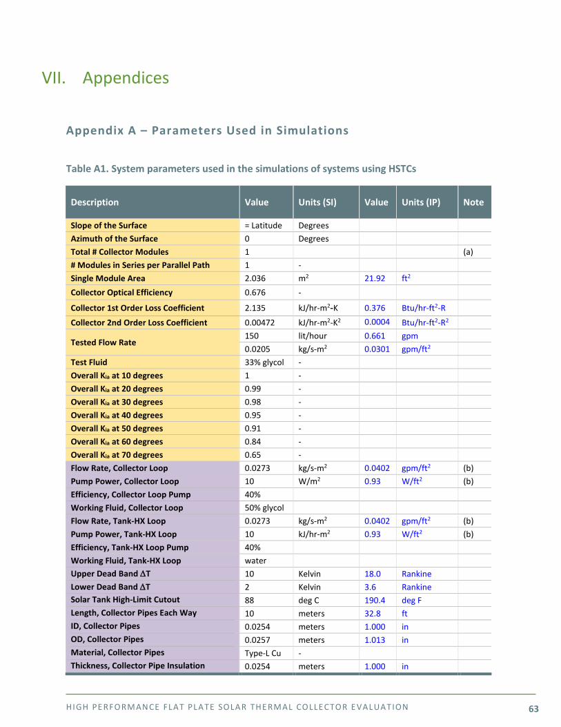
HIGH PE RFORMANCE FLAT PLATE SOLAR THE RMAL COLLE CTOR E VALUATION 63
VII. Appendices
Appendix A – Parameters Used in Simulations
Table A1. System parameters used in the simulations of systems using HSTCs
Description Value Units (SI) Value Units (IP) Note
Slope of the Surface = Latitude Degrees Azimuth of the Surface 0 Degrees Total # Collector Modules 1 (a) # Modules in Series per Parallel Path 1 - Single Module Area 2.036 m2 21.92 ft2 Collector Optical Efficiency 0.676 -
Collector 1st Order Loss Coefficient 2.135 kJ/hr-m2-K 0.376 Btu/hr-ft2-R
Collector 2nd Order Loss Coefficient 0.00472 kJ/hr-m2-K2 0.0004
Btu/hr-ft2-R2
Tested Flow Rate 150 lit/hour 0.661 gpm 0.0205 kg/s-m2 0.0301 gpm/ft2
Test Fluid 33% glycol - Overall Kia at 10 degrees 1 - Overall Kia at 20 degrees 0.99 - Overall Kia at 30 degrees 0.98 - Overall Kia at 40 degrees 0.95 - Overall Kia at 50 degrees 0.91 - Overall Kia at 60 degrees 0.84 - Overall Kia at 70 degrees 0.65 - Flow Rate, Collector Loop 0.0273 kg/s-m2 0.0402 gpm/ft2 (b) Pump Power, Collector Loop 10 W/m2 0.93 W/ft2 (b) Efficiency, Collector Loop Pump 40% Working Fluid, Collector Loop 50% glycol Flow Rate, Tank-HX Loop 0.0273 kg/s-m2 0.0402 gpm/ft2 (b) Pump Power, Tank-HX Loop 10 kJ/hr-m2 0.93 W/ft2 (b) Efficiency, Tank-HX Loop Pump 40% Working Fluid, Tank-HX Loop water Upper Dead Band ∆T 10 Kelvin 18.0 Rankine Lower Dead Band ∆T 2 Kelvin 3.6 Rankine Solar Tank High-Limit Cutout 88 deg C 190.4 deg F Length, Collector Pipes Each Way 10 meters 32.8 ft ID, Collector Pipes 0.0254 meters 1.000 in OD, Collector Pipes 0.0257 meters 1.013 in Material, Collector Pipes Type-L Cu - Thickness, Collector Pipe Insulation 0.0254 meters 1.000 in

HIGH PE RFORMANCE FLAT PLATE SOLAR THE RMAL COLLE CTOR E VALUATION 64
Description Value Units (SI) Value Units (IP) Note
Material, Collector Pipe Insulation Armaflex - Volume, Solar Storage Tank 61 lit/m2 1.50 gal/ft2 (b) Height, Solar Storage Tank 2 meters 6.6 ft Heat Loss Coeff., Solar Storage Tank 2.04 kJ/hr-m2-K 0.360 Btu/hr-ft2-R Heat exchanger effectiveness 70% - Length, Tank-HX Pipes Each Way 10 meters 32.8 ft ID, Tank-HX Pipes 0.0254 meters 1.000 in OD, Tank-HX Pipes 0.0257 meters 1.013 in Material, Tank-HX Pipes Type-L Cu - Thickness, Tank-HX Pipe Insulation 0.0254 meters 1.000 in Material, Tank-HX Pipe Insulation Armaflex - Daily Weekday Load 1892.5 Liters 500.0 gallons (a) Daily Weekend Load 72.4 Liters 19.1 gallons (a) Average Daily Load 1372.5 Liters 362.6 gallons (a) Volume, Auxiliary Tank 1.372 m3 362.6 gallons (c) Height, Auxiliary Tank 2.0 meters 6.6 ft Heat Loss Coefficient, Auxiliary Tank 2.04 kJ/hr-m2-K 0.360 Btu/hr-ft2-R Setpoint for Auxiliary Heat 60.0 deg C 140.0 deg F Deadband for Auxiliary Heat 2.5 deg C 36.5 deg F Capacity of Auxiliary Heat 100 kW Thermal Efficiency of Auxiliary Heater 100% - Desired Delivery Temperature 60.0 deg C 140.0 deg F
Notes: a. Varied over a range from one simulation to the next b. Denominator is total collector area c. Equal to average daily hot water draw
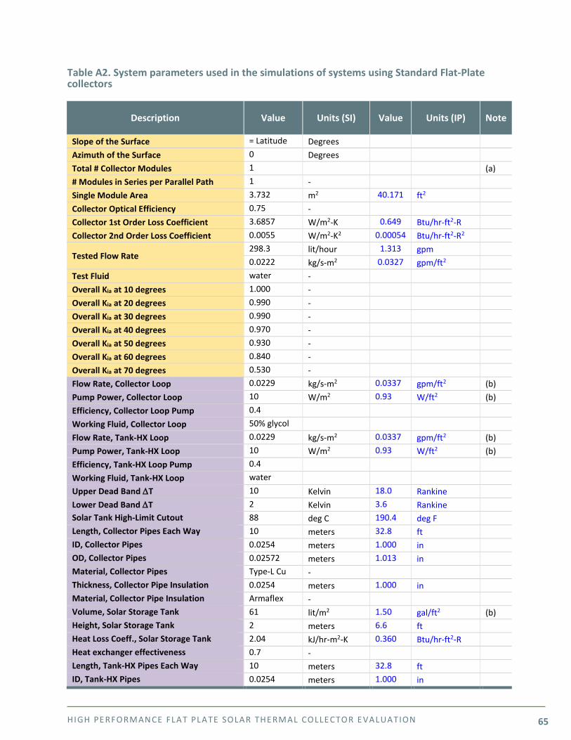
HIGH PE RFORMANCE FLAT PLATE SOLAR THE RMAL COLLE CTOR E VALUATION 65
Table A2. System parameters used in the simulations of systems using Standard Flat-Plate collectors
Description Value Units (SI) Value Units (IP) Note
Slope of the Surface = Latitude Degrees Azimuth of the Surface 0 Degrees Total # Collector Modules 1 (a) # Modules in Series per Parallel Path 1 - Single Module Area 3.732 m2 40.171 ft2 Collector Optical Efficiency 0.75 - Collector 1st Order Loss Coefficient 3.6857 W/m2-K 0.649 Btu/hr-ft2-R Collector 2nd Order Loss Coefficient 0.0055 W/m2-K2 0.00054 Btu/hr-ft2-R2
Tested Flow Rate 298.3 lit/hour 1.313 gpm 0.0222 kg/s-m2 0.0327 gpm/ft2
Test Fluid water - Overall Kia at 10 degrees 1.000 - Overall Kia at 20 degrees 0.990 - Overall Kia at 30 degrees 0.990 - Overall Kia at 40 degrees 0.970 - Overall Kia at 50 degrees 0.930 - Overall Kia at 60 degrees 0.840 - Overall Kia at 70 degrees 0.530 - Flow Rate, Collector Loop 0.0229 kg/s-m2 0.0337 gpm/ft2 (b) Pump Power, Collector Loop 10 W/m2 0.93 W/ft2 (b) Efficiency, Collector Loop Pump 0.4 Working Fluid, Collector Loop 50% glycol Flow Rate, Tank-HX Loop 0.0229 kg/s-m2 0.0337 gpm/ft2 (b) Pump Power, Tank-HX Loop 10 W/m2 0.93 W/ft2 (b) Efficiency, Tank-HX Loop Pump 0.4 Working Fluid, Tank-HX Loop water Upper Dead Band ∆T 10 Kelvin 18.0 Rankine Lower Dead Band ∆T 2 Kelvin 3.6 Rankine Solar Tank High-Limit Cutout 88 deg C 190.4 deg F Length, Collector Pipes Each Way 10 meters 32.8 ft ID, Collector Pipes 0.0254 meters 1.000 in OD, Collector Pipes 0.02572 meters 1.013 in Material, Collector Pipes Type-L Cu - Thickness, Collector Pipe Insulation 0.0254 meters 1.000 in Material, Collector Pipe Insulation Armaflex - Volume, Solar Storage Tank 61 lit/m2 1.50 gal/ft2 (b) Height, Solar Storage Tank 2 meters 6.6 ft Heat Loss Coeff., Solar Storage Tank 2.04 kJ/hr-m2-K 0.360 Btu/hr-ft2-R Heat exchanger effectiveness 0.7 - Length, Tank-HX Pipes Each Way 10 meters 32.8 ft ID, Tank-HX Pipes 0.0254 meters 1.000 in
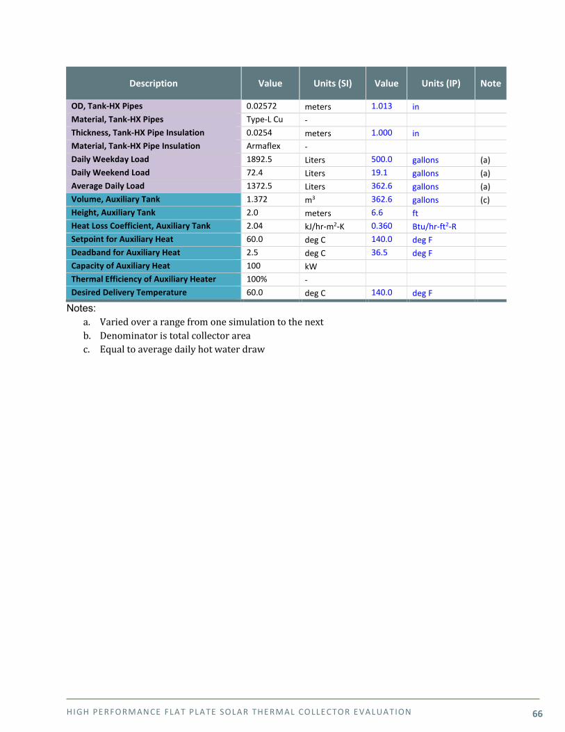
HIGH PE RFORMANCE FLAT PLATE SOLAR THE RMAL COLLE CTOR E VALUATION 66
Description Value Units (SI) Value Units (IP) Note
OD, Tank-HX Pipes 0.02572 meters 1.013 in Material, Tank-HX Pipes Type-L Cu - Thickness, Tank-HX Pipe Insulation 0.0254 meters 1.000 in Material, Tank-HX Pipe Insulation Armaflex - Daily Weekday Load 1892.5 Liters 500.0 gallons (a) Daily Weekend Load 72.4 Liters 19.1 gallons (a) Average Daily Load 1372.5 Liters 362.6 gallons (a) Volume, Auxiliary Tank 1.372 m3 362.6 gallons (c) Height, Auxiliary Tank 2.0 meters 6.6 ft Heat Loss Coefficient, Auxiliary Tank 2.04 kJ/hr-m2-K 0.360 Btu/hr-ft2-R Setpoint for Auxiliary Heat 60.0 deg C 140.0 deg F Deadband for Auxiliary Heat 2.5 deg C 36.5 deg F Capacity of Auxiliary Heat 100 kW Thermal Efficiency of Auxiliary Heater 100% - Desired Delivery Temperature 60.0 deg C 140.0 deg F
Notes: a. Varied over a range from one simulation to the next b. Denominator is total collector area c. Equal to average daily hot water draw
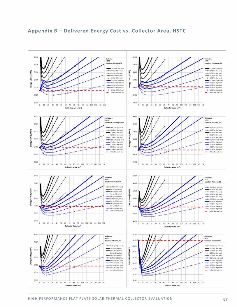
HIGH PE RFORMANCE FLAT PLATE SOLAR THE RMAL COLLE CTOR E VALUATION 67
Appendix B – Delivered Energy Cost vs. Collector Area, HSTC
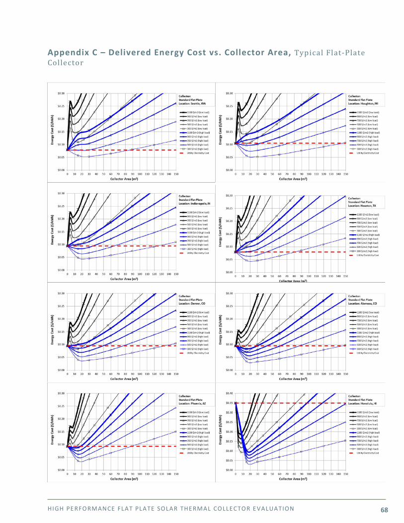
HIGH PE RFORMANCE FLAT PLATE SOLAR THE RMAL COLLE CTOR E VALUATION 68
Appendix C – Delivered Energy Cost vs. Collector Area, Typical Flat-Plate Collector
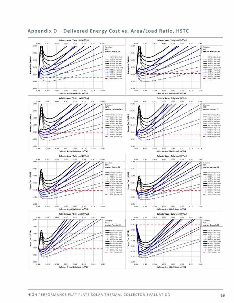
HIGH PE RFORMANCE FLAT PLATE SOLAR THE RMAL COLLE CTOR E VALUATION 69
Appendix D – Delivered Energy Cost vs. Area/Load Ratio, HSTC
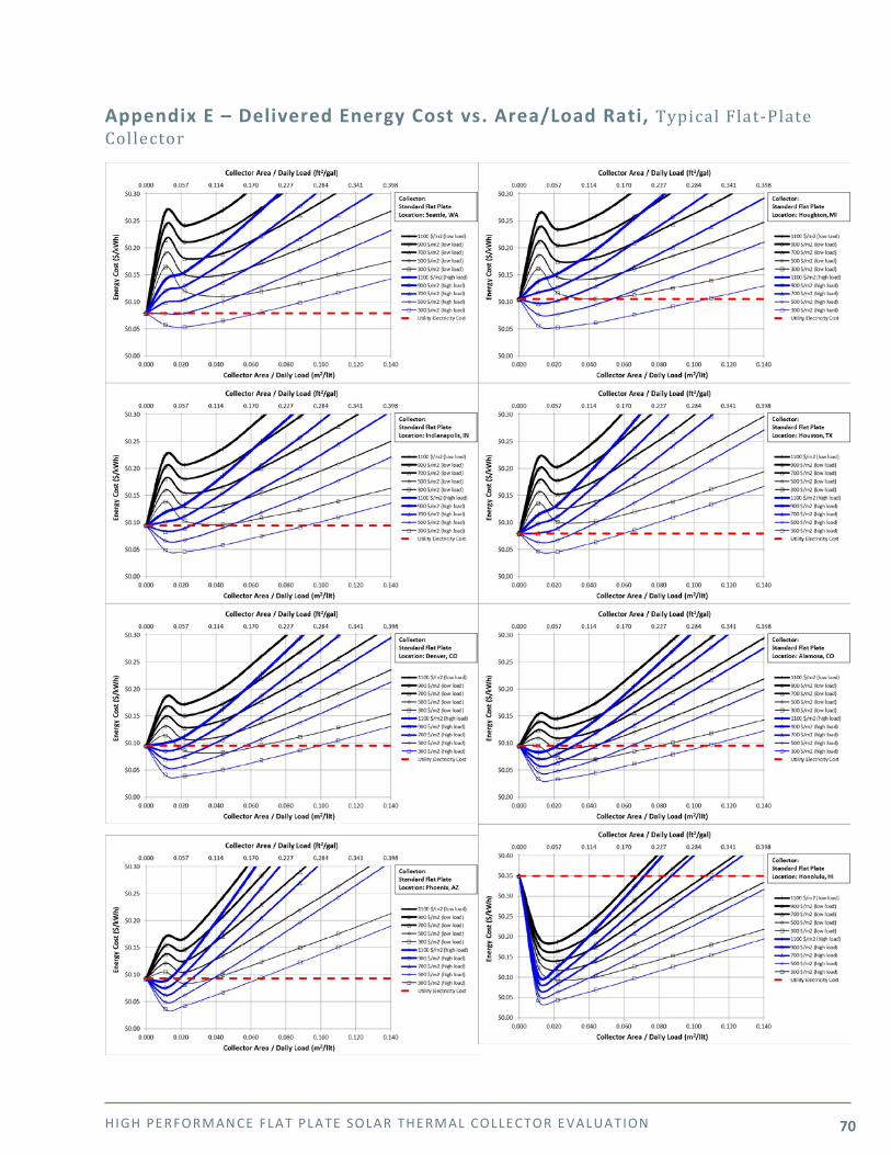
HIGH PE RFORMANCE FLAT PLATE SOLAR THE RMAL COLLE CTOR E VALUATION 70
Appendix E – Delivered Energy Cost vs. Area/Load Rati, Typical Flat-Plate Collector
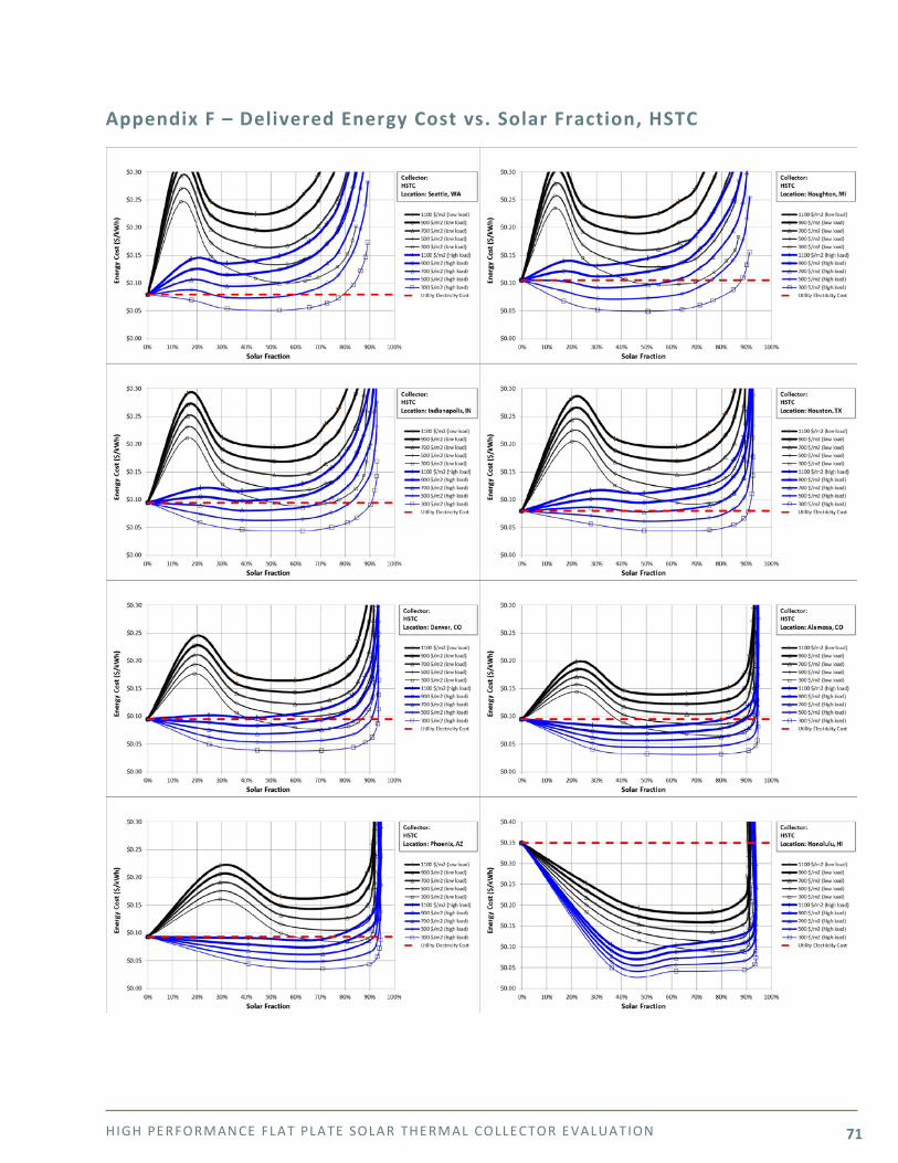
HIGH PE RFORMANCE FLAT PLATE SOLAR THE RMAL COLLE CTOR E VALUATION 71
Appendix F – Delivered Energy Cost vs. Solar Fraction, HSTC
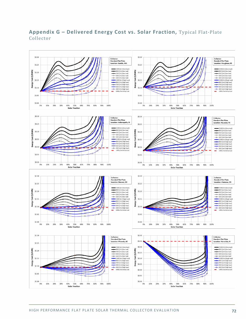
HIGH PE RFORMANCE FLAT PLATE SOLAR THE RMAL COLLE CTOR E VALUATION 72
Appendix G – Delivered Energy Cost vs. Solar Fraction, Typical Flat-Plate Collector

HIGH PE RFORMANCE FLAT PLATE SOLAR THE RMAL COLLE CTOR E VALUATION 73
Appendix H – Comparisons of Delivered Energy Costs, HSTC vs. Standard Flat-Plate Notes:
• For the purpose of comparing performance, installed costs for HSTC and Standard Flat Plate systems are assumed to be equal on a per-collector-area basis
• Application is heating of mains temperature water to 60oC (140oF) • Performance is nearly independent of climate temperature • There are typically two possible goals in designing a properly-sized system: (1) lowest delivered
energy cost (blue circle) and (2) highest amount of delivered energy while remaining cost-effective over the system’s lifetime (yellow circle).
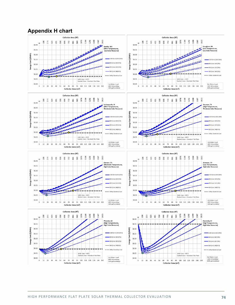
HIGH PE RFORMANCE FLAT PLATE SOLAR THE RMAL COLLE CTOR E VALUATION 74
Appendix H chart
HIGH PE RFORMANCE FLAT PLATE SOLAR THE RMAL COLLE CTOR E VALUATION 75
Appendix I – Nomenclature
Ac Total aperture area of the collector array (m2)
Ca Area-dependent cost of SHW system ($/m2)
Ccap Annualized capital cost of the system ($/year)
Cdel Cost of delivered energy over the life expectancy of the system ($/kWh)
Ce Annualized cost of electrical energy ($/year)
Cf Fixed cost of SHW system ($)
Ci Total installed cost of SHW system ($)
Ci-life Annual payment on a loan for installed cost of SHW system ($)
Co&m Annual operation and maintenance cost ($/year)
Co&m-life Average annual O&M cost over life expectancy of the system, including inflation ($/year)
Cp Specific heat of collector fluid (J/kg-K)
Cu Unit cost of electrical energy ($/kWh)
Cu-life Average unit cost of energy over the life expectancy of the system, including fuel cost escalation ($/kWh)
Edel Total energy added to water (kWh/year)
Ee Total electrical energy used by system (kWh/year)
Es Total energy saved by the solar system (kWh/yr)
FR Correction factor to allow prediction of performance using Ti (unit less)
fs Solar fraction
Ig Global solar radiation in the plane of the collector array (W/m2)
Kia Incidence angle modifier, Kia = 1.0 at normal incidence (unit less)
mcoll Mass flow rate of collector fluid (kg/sec)
qcoll Total rate of energy delivery by the collector array (W)
qcoll,m Total rate of energy delivery by the collector array, measured (W)
Qns Total energy used to heat hot water, no SHW system (kWh/year)
HIGH PE RFORMANCE FLAT PLATE SOLAR THE RMAL COLLE CTOR E VALUATION 76
qpred Total rate of energy delivery by the collector array, predicted (W)
Qns Total energy used to heat hot water, with SHW system (kWh/year)
Ta Ambient air temperature near collector array (oC)
Ti Temperature of fluid entering collector array (oC)
To Temperature of fluid exiting collector array (oC)
Tm Mean temperature of collector fluid, calculated as (Ti + To)/2 (oC)
UL1 First-order heat loss coefficient (W/m2-K)
UL2 Second-order heat loss coefficient (W/m2-K2)
Vcoll Volume flow rate of collector fluid (lit/sec)
Vdhw Average daily volume of hot water drawn through system (lit)
η Efficiency (unitless)
ηmeas Efficiency (measured)
ηpred Efficiency (predicted)
ηο Optical efficiency (unitless)
ρcoll Density of collector fluid (kg/lit)
θi Beam incidence angle
(τα) Transmittance-absorptance product, equal to ηο
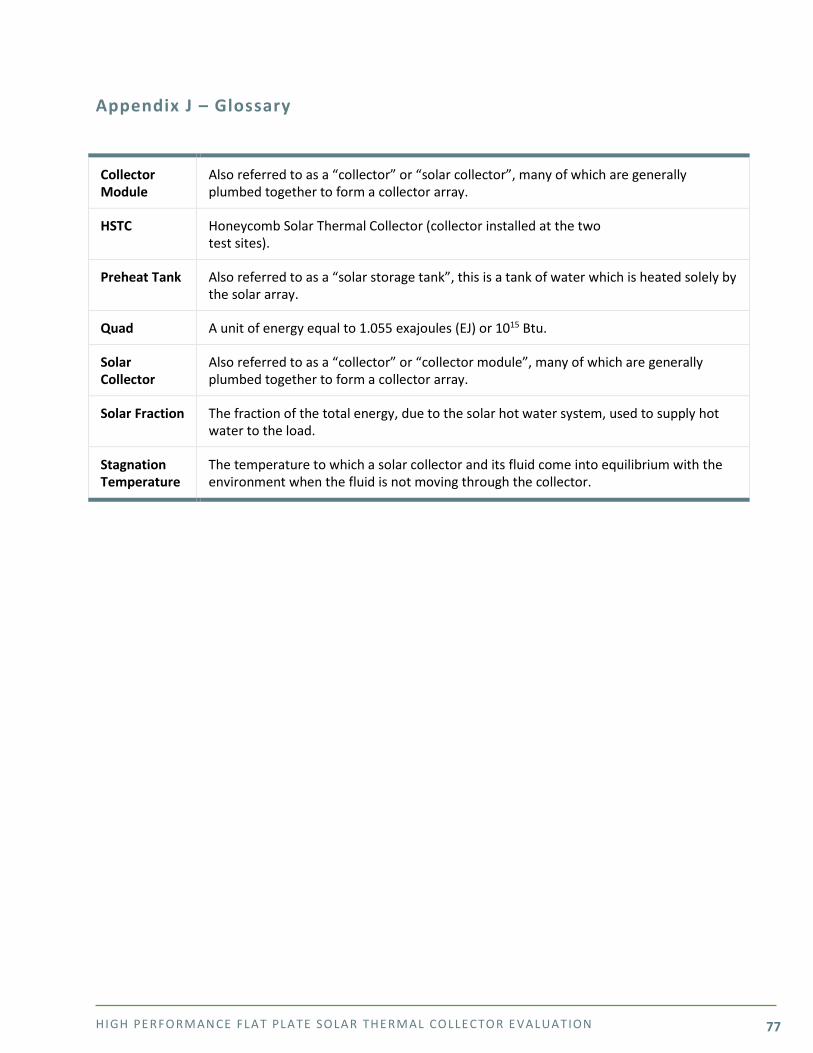
HIGH PE RFORMANCE FLAT PLATE SOLAR THE RMAL COLLE CTOR E VALUATION 77
Appendix J – Glossary
Collector Module
Also referred to as a “collector” or “solar collector”, many of which are generally plumbed together to form a collector array.
HSTC Honeycomb Solar Thermal Collector (collector installed at the two test sites).
Preheat Tank Also referred to as a “solar storage tank”, this is a tank of water which is heated solely by the solar array.
Quad A unit of energy equal to 1.055 exajoules (EJ) or 1015 Btu.
Solar Collector
Also referred to as a “collector” or “collector module”, many of which are generally plumbed together to form a collector array.
Solar Fraction The fraction of the total energy, due to the solar hot water system, used to supply hot water to the load.
Stagnation Temperature
The temperature to which a solar collector and its fluid come into equilibrium with the environment when the fluid is not moving through the collector.
HIGH PE RFORMANCE FLAT PLATE SOLAR THE RMAL COLLE CTOR E VALUATION 78
Appendix K – References
[1] EIA Solar Thermal Collector Manufacturing Activities 2009, available at: http://www.energybc.ca/cache/solarthermal/www.eia.gov/renewable/annual/solar_thermal/solar.html
[2[ Klein, Beckman, et al., TRNSYS – A Transient System Simulation Program, Solar Energy Laboratory,
University of Wisconsin, Madison, WI, http://sel.me.wisc.edu/trnsys/. [3] Walker, Andy, Solar Energy – Technologies and Project Delivery for Buildings, John Wiley & Sons, 2013,
http://www.wiley.com/WileyCDA/WileyTitle/productCd-1118139240.html. [4] Walker, Andy, “Solar Water Heating,” 7th Annual North American Passive House Conference, Sept. 27-30,
2012, Denver, CO, http://www.nrel.gov/docs/fy13osti/56706.pdf.
[5] Department of Energy, Office of Energy Efficiency and Renewable Energy, ENERGY ESCALATION RATE CALCULATOR, http://energy.gov/eere/femp/energy-escalation-rate-calculator-download.
[6] Solartechnik Prufung Forschung, “Report on Accelerated OPD Test TIGI Collector Grand Summary”, Nov.
16, 2014. [7] Frank, Mauthner, Fischer, “Overheating Prevention and Stagnation Handling in Solar Process Heat
Applications,” IEA SHC Task 49, Solar Process Heat for Production and Advanced Applications, Technical Report A.1.2, January 15, 2015.
[8] Solartechnik Prufung Forschung, “Test Report No. C1493LPEN,” October 16, 2012. [9] Source for average electricity rates by state: http://energy-models.com/tools/average-electric-and-gas-
cost-state. [10] Christensen, C. and Barker, G., “Annual System Efficiencies for Solar Water Heating”, Proceedings of the
1998 American Solar Energy Society Conference, 14-17 June 1998, Albuquerque, New Mexico, pp. 291-296.