high power loss reduction in enugu … · n39,500.00 per year after amortizing the ... figure 2.8...
TRANSCRIPT

1
HIGH POWER LOSS REDUCTION IN ENUGU ELECTRICAL DISTRIBUTION SYSTEMS USING HEURISTIC TECHNIQUE FOR CAPACITOR PLACEMENT.
A PROJECT SUBMITTED TO THE DEPARTMENT OF ELECTRICAL ENGINEERING IN PARTIAL FULFILMENT
OF THE REQUIREMENT FOR THE AWARD OF MASTER OF
ENGINEERING (M.ENG) DEGREE.
BY
UZODIFE NICHODEMUS ANAYO PG/M. ENG/03/34636
SUPERVISOR: VEN. ENGR. PROF. T.C. MADUEME
UNIVERSITY OF NIGERIA NSUKKA
MAY 2009.

2
APPROVAL PAGE
HIGH POWER LOSS REDUCTION IN ENUGU
ELECTRICAL DISTRIBUTION SYSTEMS USING HEURISTIC TECHNIQUE FOR CAPACITOR PLACEMENT.
PROJECT WORK PRESENTED IN FULFILLMENT OF THE REQUIREMENTS FOR THE AWARD OF MASTER OF ENGINEERING DEGREE (M.ENG) IN ELECTRICAL
ENGINEERING
BY
MR. UZODIFE NICHODEMUS ANAYO PG/M. ENG/03/34636
DEPARTMENT OF ELECTRICAL ENGINEERING UNIVERSITY OF NIGERIA NSUKKA
AUTHOR ___________________________ UZODIFE NICHODEMUS ANAYO
SUPERVISOR ___________________________ ENGR. PROF. T.C. MADUEME
HEAD OF DEPARTMENT ___________________________
ENGR. DR. L.U. ANIH EXTERNAL EXAMINER ___________________________
ENGR. PROF. J.C. EKEH

3
DECLARATION
I declare that the work is original and has not been submitted
elsewhere for the purpose for the award of Degree to the best of my
knowledge.
_________________________________
UZODIFE NICHODEMUS ANAYO
AUTHOR

4
CERTIFICATION
UZODIFE NICHODEMUS ANAYO, a postgraduate student in the
Department of Electrical Engineering, with Registration Number
PG/M.ENG/03/34636 has satisfactorily completed the requirements for
the course and research work for the Degree of Master of Engineering
(M. Eng.) in the Department of Electrical Engineering, University of
Nigeria Nsukka.
The work embodied in the dissertation is original and has not been
submitted in part or full for any other diploma or degree of this university
or other institution to the best of our knowledge.
___________________________ ________________________
Ven. Engr. Prof. T.C. Madueme Engr. Dr. L.U. Anih
Supervisor Head of Department

5
DEDICATION
This project is dedicated to:
My father, Chiekpote Uzodife, for a lifetime of love and support,
which, while not always spoken was always understood and
remembered.
Jesus, your love for life is an inspirations. You will be always close
to my heart.

6
ACKNOWLEDGEMENT
In the first place, I would love to show my gratitude towards God
the father and the giver of life.
Sincerely, I acknowledge and thank Ven. Engr, Prof. T.C. Madueme
my lecturer and my supervisor in master’s degree programme for his
immense contributions.
My thanks and acknowledgement go to Engr. Prof. M.U Agu, Dr.
L.U. Anih, Prof. O.I Okoro, Dr. E.S Obe, Engr. B.O Anyaka and other
lecturers and staff of Electrical Department, University of Nigeria,
Nsukka (UNN).
My thanks and acknowledgement is also extended to the staff of PHCN
(Transmission and Distribution) sectors for their contribution to the
success of my project. People like. Engr. Akamunonu (C.E.O), Engr
Albert .U. Esenabhalu, Engr. CY. Umeigbo, Engr. Aniagu, Engr. E.I.
Anene, Engr. Bakari and other PHCN staff cannot be forgotten for their
contributions towards the success of the work.

7
ABSTRACT
This project involves research on loss reduction in a distribution
system. The Enugu distribution system is the case study. The type of
losses, the causes of losses and methods of loss reduction in distribution
system were presented. A method based on a heuristic technique for
reactive loss reduction in distribution system is chosen for this work
because it provides realistic sizes and locations for shunt capacitors on
primary feeder at a low computational burden. The Gauss-siedel method
was used for load analysis while simulation work was done using
MATLAB software. The variation of the load during the year is
considered. The capital and installation cost of the capacitors are also
taken into account. The economical power factor is also determined so
as to achieve maximum savings. This method is applied to a 34 bus,
11KV, 6MVA distribution system with original power factor of 0.85. The
results from the analysis show that the losses are reduced from 59.2692
to 49.4KW using capacitor maximum rating of 1200 (750+450) KVAR at
an optimum power factor of 0.96. This translates to a saving of
N39,500.00 per year after amortizing the capital and installation costs of
applying the compensating capacitors.

8
TABLE OF CONTENT
Cover Page i
Approval Page ii
Declaration iii
Certification iv
Dedication v
Acknowledgment vi
Abstract vii
Table of Contents viii
List of Symbols and Abbreviations xi
List of Figures xiii
List of Tables xv CHAPTER ONE: INTRODUCTION
1.1 Background of the Study 1
1.2 Motivation and Significance of the study 3
1.3 Aim and Objectives 4
1.4 Methodology 4
1.4.1 Sources of Data. 5
1.4.2 Techniques to be employed. 5
1.4.3 Instrument to be employed. 5
1.4.4 Tools to be employed. 6
1.5 Project Organization. 6
CHAPTER TWO: ELECTRICAL DISTRIBUTION LOSSES AND APPLICATION OF
CAPACITORS:
2.1 Sources of Losses in Electrical Distribution Systems 7
2.1.1 Losses in Distribution Lines 7
2.1.2 Losses in Distribution Transformer 9

9
2.1.3 Type of Losses in Distribution Systems 11
2.2 Causes of Technical Losses in Distribution Systems 11
2.3 Causes of Losses in Distribution Feeders 13
2.4 Methods of Loss Reduction in Distribution Systems 15
2.5 Application of Power Capacitors to Electrical Distribution Systems 21
2.6 Effect of Series and Shunt Capacitors in Electrical Distribution
Systems 22
2.7 Power Factor Corrections 24
2.7.1 Capacitive Power Factor Corrections 27
2.7.2 Theoretical Method of Capacitive Power Factor Corrections 28
2.7.2.1 Permanently 28
2.7.2.2 Controlled 31
2.7.2.3 At The Motors 31
2.7.3 Methods of Identifying Power Factors in Distribution Systems 32
2.7.4 Convenient Calculation Methods for Capacitive Power Factor
(PF) Improvement 34
2.7.5 Compensation Theory for Capacitive Power Factor Correction 37
2.7.6 Power Loss Reduction Using Capacitor 47
2.7.7 Consideration of Harmonics when Applying Capacitors 48
2.7.8 Cardinal Rules for Application of Capacitor Banks in Distribution Systems 51
2.8 Active Power Factor Correction 52
2.8.1 Boost Circuit Parameter Optimization 55
2.8.2 Value of the Input Capacitor C1 55
2.8.3 Current Ripple in the Boost Inductor 55
2.8.4 Principles of Operation of Active Power Factor Correction
Technique for Three-Phase Diode Rectifiers 57
2.9 Properties of Capacitive and Active Power Factor Correction 61
2.10 Comparison of Capacitive and Active Power Factor Corrections 62

10
CHAPTER THREE LOAD FLOW ANALYSIS AND SYSTEM MODELLING
3.1 System modeling 64
3.2 Load flows 64
3.3 Node equations 66
3.4 Load variation with time 77
3.5 Derivation of power loss reduction equations 78
3.5.1 I2R Loss Reduction Due to Capacitor 80
3.6 Derivation of economical power factor 82
CHAPTER FOUR: APPLICATION OF THE PROPOSED METHOD 4.1 Load Flow Results 91
4.2 Results Analysis 96
CHAPTER FIVE: CONCLUSION AND RECOMMENDATIONS 5.0 Conclusion 108
5.1 Recommendations 108
References 111
Appendix I 115
Appendix II 118

11
LIST OF SYMBOLS AND ABBREVIATIONS ABBREVIATIONS
KVA - Kilovaltamperes
KV - Kilovolt
Pf - Power Factor
Ci - Cost per kilvar of capacitor bank
Si - Cost per kilovolt amperes of system equipment
V - Percentage voltage rise of the joint of capacitor installation
Kv - System line to line voltage without capacitor in service
Kvar - Kilovolt ampere reactive.
KL - Inductive reactance of the system at the point of the
capacitor installation, in ohms.
KW - Kilowatts
P.H.C.N - Power Holding Company of Nigeria
VAr(C) - Capacitor Reactive Power
AC - Alternating Current
S - Apparent power
Q - Reactive Power
P - True Power
X - Reactance
Xc - Capacitive Reactance
C - Capacitance of Capacitor
h - Resonant frequency
SMPS - Switch mode power supply
APFC - Active power factor correction
Yio and Yjo - Reactive Shunts respectively
GSLF - Gauss-siedel Load flow
Y-bus - Admittance bus

12
Ic - Capacitor Current
PL - Amount of power lost
I - Current
R - Resistance
S - Real and reactive power load level
V - Voltage Line
- Resistivity
L - Length of line
A - Cross sectional area
GRA - Government Reserved Area
SYMBOLS
- Capacitor
- Inductor
- Transformer
- Contactor switch
- Motor
- Motor
- Resistor
- Capacitor
M

13
LIST OF FIGURES
Figure 2.1 - Lagging Power Factor 26
Figure 2.2 - Leading Power Factor 26
Figure 2.3 - (a) and (b) Parallel (shunt) connection
capacitors in Luminaire 29
Figure 2.4 - Series Connection of capacitors in Luminaire 30
Figure 2.5 - Standard power factor Correction 31
Figure 2.6 - Capacitors connected to 3 Phase Motor 32
Figure 2.7 - Power Triangle 33
Figure 2.8 - Right-triangle relationship calculation in a.c. circuit 34 Figure 2.9 - Power Factor Correction (a – e) 37
Figure 2.10 - Capacitive Power Loss Reduction 47
Figure 2.11 - Addition to Harmonic Filters 50
Figure 2.12 - Basic Topology of a Boost PFC 54
Figure 2.13 - Basic Active Power Factor Correction Circuit 56
Figure 2.14 - (a) Proposed three-phase ac to dc converter (b) Single-phase equivalent circuit of (a) 58
Figure 2.15 - Simulated waveforms. (a) Three-phase voltages (b) Boost switch bQ gating signals.
(c) Rectifier input current iaI 59
Figure 3.1 - Simple electric circuit 66
Figure 3.2 - equivalent for line charging 68
Figure 3.3 - On line diagram of 4 bus distribution system 69
Figure 3.4 - Nominal - circuit 73
Figure 3.5 - Fig. 3.5 Effect of capacitor in parallel with an
inductive load:
(a) an inductive load,
(b) adding a capacitor 80
14
Figure 3.6 - Power triangle for Economical power factor
and net savings 82
Figure 4.1 - One – Line Diagram of 34 Bus Thinker’s Corner
Distribution System with Laternal Branches 88
Figure 4.2 - Graph of Power Loss and Loss Reduction
Versus Size of Capacitor Bank on Node 26 only 100
Figure 4.3 - Graph of Power Loss and Loss Reduction
Versus size of Capacitor Banks on Node 11 only 101
Figure 4.4 - Graph of Power Loss & Loss Reduction Versus
Total Size of Capacitor Banks on Nodes 26 and 11 102
Figure 4.5 - Graph of Savings per annum Versus Total
Size of Capacitor Banks on Nodes 26 only 103
Figure 4.6 - Graph of Savings per annum Versus Total
Size of Capacitor Banks on Nodes 11 only 104
Figure 4.5 - Graph of Savings per annum Versus Total
Size of Capacitor Banks on Nodes 26 and 11 105

15
LIST OF TABLES
Table 2.1 - Rated reactive power of the compensator
Required for full compensation per unit
rated apparent power of the load and power
unit real power of the load for various power
factors by which the losses are increased. 41
Table 3.1 - Classification of Load Flow Buses 66
Table 3.2 - y-bus 72
Table 4.1 - Thinker’s Corner 11kv Feeder line distribution
system data 89
Table 4.1.1 - Bus Data 89
Table 4.1.2 - Line Data 90
Table 4.1.3 - Voltages and Currents in the Distribution System 91
Table 4.1.4 - Calculated power losses in the system due to
active and reactive component of current
before compensation 92
Table 4.1.5 - Power losses due to reactive component of load
current before compensation (pf.= 0.85) 93
Table 4.1.6 - Power Losses and Loss Reduction due to
Addition of Capacitor Banks on Nodes 26, 11,
and the overall Power Losses and loss
reduction due to capacitor banks on
nodes 26 and 11 combined 94
Table 4.1.7 - Power Factor and Savings due to the addition of
capacitor banks on nodes 26, 11 and nodes
26 and 11 combined 95
16
CHAPTER ONE
INTRODUCTION
1.1 BACKGROUND OF STUDY
Electrical distribution systems include the distribution of electrical
energy for light and power from the point of generation to the point of
utilization [1].
Distribution of energy is accomplished in this project by the use of a.c
system. Distribution system consists of two parts: the primary distribution
which extends either from the generating station or substatio00n to
distribution transformers, and the secondary distribution, which extends
from the distribution transformers to the point of utilization. An electrical
distribution system can normally be of overhead or underground
construction. The overhead construction is generally used in Enugu
because it offers the following advantages.
I It is less expensive
II It is easier to identify and repair fault
Overhead distribution system is accomplished by means of two
types of conductors: the bare conductors and insulated conductors. The
bare conductors are those used for long distribution lines while the
insulated conductors are those used for short distribution lines. The
insulated conductors are also called service cables. They are used
between poles and houses so as to prevent electric shock incase the
conductor gets in contact with any of the metals in the building.
Enugu Electrical system receives its energy from Onitsha at
330kV. The 330kV is stepped down to 132kV in Onitsha and transmitted
from Onitsha to New-Haven transmission station. At New-Haven
transmission station the 132kV was stepped down to 33kV and
transmitted to the following injection substations in Enugu: Kingsway,
Independent Layout, Thinkers Corner, 9th Mile, Ituku Ozara and Emene

17
Industrial Layout. At the injection substations, the 33kV is further
stepped down to 11kV and distributed to various areas in Enugu. In this
project, the loss reduction in 11kV Thinkers Corner distribution line will
be considered [1].
The power network, which generally concerns the common man, is
the distribution network of 11kV lines or feeders downstream of the 33kV
substation. Each 11kV feeder which emanates from the 33kV substation
branches further into several subsidiary 11kV feeders to carry power
close to the load points (localities, industrial areas, villages, etc.). At
these load points, a transformer further reduces the voltage from 11kV to
415V to provide the last-kilometer connection through 415V feeders
(also called as Low Tension (LT) feeders) to individual customers in
Enugu, either at 240V (as single-phase supply) or at 415V (as three-
phase supply). The span lengths mainly used for electricity projects
nationwide are 45/50 meters for Township Distribution Network (TDN)
and between 65 and 90 meters for inter-township connection (ITC) lines.
In Enugu State, the average span length for both 11kV and 415V
distribution lines is 50 meters between two poles.
After electric power is generated, it is sent through the
transmission lines to the many distribution circuits that the utility
operates. The purpose of the distribution system is to take that power
from the transmission system and deliver it to the consumers to serve
their needs. However, a significant portion of the power that a utility
generates is lost in the distribution process. These losses occur in
numerous small components in the distribution system, such as
transformers and distribution lines. Due to the lower power level of these
components, the losses inherent in each component are lower than
those in comparable components of the transmission system. While
each of these components may have relatively small losses, the large

18
number of components involved makes it important to examine the
losses in the distribution system [2].
There are two major sources of losses in power distribution
systems. These are the transformers and distribution lines. Additionally,
there are two types of losses that occur in these two components. These
losses are often referred to as core losses and copper, or I2R, losses. In
the case of transformers, the core losses account for the majority of
losses at low power levels. As load increases, the copper losses become
more significant, until they are approximately equal to the core losses at
peak load [2].
The economic implications of these losses are far reaching. In
addition to the excess fuel cost needed to cover the energy, added
generating capacity may be needed. Also, the power lost in the
distribution system must still be transmitted through the transmission
system which further adds to the loss in that system. It is very important
for electric power suppliers to consider these losses and reduce them
wherever practical.
1.2 MOTIVATION AND SIGNIFICANCE OF THE STUDY
Initially, as power factor falls below unity the current in the system
increases with the following effects:
(i) Because of the increased currents, the I2R power loss
increases in cables and windlings leading to overheating and
consequent reduction in equipment life.
(ii) Cost incurred by power company increases.
(iii) Efficiency as a whole suffers because more of the input is
absorbed in meeting losses.
Since distribution losses cost the utilities a very big amount
of profit, reduce life of equipment, attempts to reduce electricity
cost, together with improving the efficiency of distribution systems,

19
have led us to deal with the problem of power loss minimization.
The system is considered as efficient when the loss level is low.
The significance of the expected outcome of the study include the
following:
(i) It ensures that the rated voltage is applied to motors, lamps,
etc, to obtain optimum performance.
(ii) It decreased loses in circuits and cables
(iii) It ensures maximum power output of transformers is utilized
and not used in making-up losses.
(iv) It enables existing transformers to carry additional load
without overheating or the necessity of capital cost of new
transformers.
(v) It achieves the financial benefits which will result from lower
maximum demand charges.
1.3 AIM AND OBJECTIVES
The major aim or purpose of the research effort is to reduce
power losses in the 11Kv distribution system, achieve efficiency
and financial benefits which will result from lower maximum
demand charges by the electricity supply company.
The objectives of the research project are:
(i) To find the power losses in the distribution system and
(ii) To find means to reduce the losses and reduce them.
Once the objectives are properly carried out the aims will be
achieved.
1.4 METHODOLOGY
Since the project topic embraces determination of High Power
Loss Reduction in distribution lines, effort will be made to explain how
materials were obtained for this research project.

20
The research design object being descriptive and explorative will involve
theoretical and mathematical model analysis.
The methodology or systems of actualizing the project are as follows:
1.4.1 SOURCES OF DATA:
Sources of data for this research work under review are based
on visits made to Power Holding Company of Nigeria (PHCN) to find
how losses occur, how to reduce it and how to assess the most
economical method of loss reduction computation.
Data collection was obtained at PHCN Distribution Zonal Head
Quarters Okpara Avenue, New Haven Transmission station and
Thinker’s Corner injection substation Enugu.
1.4.2 Techniques to be employed to achieve the objectives are as
follows:
(i) Derivation of power loss reduction equations
(ii) Derivation of economic power factor. Economic power factor
is the power factor at which the savings is maximum.
(iii) Heuristic technique for capacitor placement. This is the
method of allocating capacitors at the sensitive nodes.
Sensitive node is the node that has the largest power loss
due to reactive component of load current.
(iv) Load flow technique in MATLAB should be employed as the
software for the study.
1.4.3 The instruments employed in the study are as follows: Ammeter,
Voltmeter, Wattmeter, Clip on Ammeter, Digital multimeter and
Power factor meter.
More specifically, capacitor banks are required at
locations where field measurements indicate a low voltage or

21
low power factor problem. This information can be obtained
as follows:
(a) By making voltage measurements during full-load (Peak-
load) and light-load (off peak-load) conditions at various
points on the distribution feeder; and
(b) By making kilowatt and kilovoltampere measurements on the
distribution feeder at minimum and maximum daily loads and
during a typical 24 hour period.
Once these measurements have been obtained, equation 2.41 can
be used to determine voltage rise and kilovar parameters. The capacitor
banks may be connected grounded star (wye), ungrounded star (wye),
or delta.
1.4.4 The tools employed in the study are, set of spanners, set of
screwdrivers and pliers. 1.5 PROJECT ORGANIZATIONS
Chapter one states the objective and serves as introduction to this
project.
Chapter two presents the theory necessary to understand and
meet the objective. It presents the reactive power control problems.
Chapter three, presents the system model and problem
formulation adopted in this project and describes the solution
methodology in detail.
Chapter four, presents the application of the solution methodology.
It also discusses the results obtained when this methodology was
applied to a test distribution system.
Finally, chapter five, provides conclusion and recommendations for
future work.

22
CHAPTER TWO ELECTRICAL DISTRIBUTION LOSSES AND APPLICATION OF CAPACITORS
Electrical distribution losses are the losses due to copper and
cores in distribution systems.
2.1 SOURCES OF LOSSES IN ELECTRICAL DISTRIBUTION SYSTEMS
There are two major sources of losses in electrical distribution
systems. These are the transformers and distribution lines.
2.1.1 LOSSES IN DISTRIBUTION LINES
One of the major sources of losses in the distribution system is the
power lines which connect the substation to the loads. Virtually all real
power that is lost in the distribution system is due to copper losses.
Since these losses are a function of the square of the current flow
through the line, it should be obvious that the losses in distribution lines
are larger at high power levels than they are at lower levels.
Since power loss in the distribution lines can be considered to be
entirely due to copper losses, it can be calculated using Equation 2.1.
PL = I2R 2.1
From this, it is apparent that anything, that changes either current
(I) or line resistance (R) will affect the amount of power lost (PL) in the
line.
The primary determining factor for the magnitude of line current is
the amount of real and reactive power loading at the end of the line. As
the power that is transmitted along the line increases, the current flow in
the line becomes larger. Another factor which affects the level of current
flow is the operating voltage of the line. For a given real and reactive
power load level, S, a high voltage line will have a lower current than a
low voltage line. This can be seen from Equation 2.2

23
S-VI 2.2
Therefore, for a given power level, the higher voltage (V) line will
have lower copper losses.
Another factor which can result line losses is unbalanced loading.
If one of the phases is loaded more heavily than the others, the loss will
be larger than it would have been in the balanced load case. This is due
to the squaring of the current in Equation 2.1
While the current level has the biggest effect on line loss, the
resistance of the line cannot be neglected. The line resistance depends
on many factors, including the length of the line, the effective cross-
sectional area, and the resistivity of the metal of which the line is made.
The resistance is inversely proportional to the cross-sectional area and
directly proportional to both the length and resistivity. This is shown in
Equation 2.3 below, where R is the resistance, is the resistivity, L is
the length of the line, and A is the effective cross-sectional area.
ALR 2.3
Therefore, a long line will have a higher resistance and larger
losses than a short line with the same current flow. Similarly, a large
conductor size results in a smaller resistance and lower losses than a
small conductor.
The resistivity is determined by the material of which the line is
constructed and the temperature of the material. A better conducting
material will result in lower resistivity and lower losses. The resistivity of
the metal in the line will be affected by the temperature. As the
temperature of the metal increases, the line resistance will also increase,
causing higher copper losses in the distribution line. The resistivity of
copper and aluminium can be calculated from Equation 2.4

24
o
o
TTTT
1
221 2.4
The letter rho, , is the resistivity at a specific temperature. It is
equal to 81083.2 ohm meters for aluminium and 81077.1 ohm meters
for copper at a temperature of 20oC. T0 is a reference temperature and is
equal to 228oC for aluminium and 241oC for copper. 1 and 2 are the
resistivities at temperature T1 and T2 respectively [3].
2.1.2 LOSSES IN DISTRIBUTION TRANSFORMERS
While losses in distribution lines are virtually all due to copper
losses, transformer losses occur due to both copper and core losses.
The core losses are made up of eddy current and hysteresis losses. The
copper losses in transformers are essentially the same as those in the
power distribution lines.
The copper losses in a transformer are smaller in magnitude than
the core losses. These losses occur in the form of heat produced by the
current, both primary and secondary, through the windings of the
transformer. Like the copper loss in the distribution line, it is calculated
using the I2R relationship of Equation 2.1. Any factor which affects either
current or winding resistance will also affect the amount of copper loss in
the transformer.
An increase in loading, either real or reactive, will result in an
increase in current flow and a correspondingly greater amount of loss in
the transformer. Additionally, an unbalanced system load will increase
transformer loss due to the squared current relationship. The winding
resistance also has an affect on the amount of copper loss and is mainly
determined by the total length of the wire used, as well as the size of the
wire. Temperature of the winding will affect the resistivity of the wire,
25
therefore affecting the overall resistance and the copper loss. Since all
but the smallest distribution transformers have some type of cooling
system, such as immersion in oil, the temperature effect on losses is
usually minimal.
The core loss in a transformer is usually larger in magnitude than
the copper loss. It is made up of eddy current losses, which are due to
magnetically induced currents in the core, and hysteresis losses, which
occur because of the less than perfect permeability of the core material.
These losses are relatively constant for an energized transformer and
can be considered to be independent of the transformer load.
Transformer core losses have been modeled in various ways, usually as
a resistance in parallel with the transformer’s magnetizing reactance [3]
[4] [5].
Since the core loss is relatively independent of loading, the most
important factor when considering core loss is the manufacture of the
core. The physical construction of the core has serious consequences
on the amount of core loss occurring in the transformer. For instance,
eddy currents are greatly reduced by using laminated pieces to construct
the core. These thin sheets are oriented along the path of travel of the
magnetic flux and restrict the amount of reduced currents that occur. [4]
The hysteresis loss occurs in the transformer core due to the
energy required to provide the magnetic filed in the core as the direction
of magnetic flux alternates with the alternating current wave form. This
energy is transformed into heat. Hysteresis loss can be reduced by the
use of higher quality materials in the core which have better magnetic
permeability [6] [7].
A final aspect of the distribution system that increases losses in
the transformers is the presence of harmonics in the system. The
harmonic currents only cause a small increase in copper losses

26
throughout the system. However, the high frequently harmonic voltages
can cause large core losses in the transformer. Frequently, utilities are
forced to use an oversized transformer to compensate when a large
harmonic presence is indicated. The increased skin effect of larger
conductors combined with the high frequency harmonics can result in
even greater losses [8].
2.1.3 TYPES OF LOSSES IN DISTRIBUTION SYSTEMS
The types of losses in distribution system are commercial and
technical losses.
Commercial losses are losses due to non-issuance of bills, due to
non-reading of meters, use of inappropriate billing methods, losses that
could result from the use of load limiters and power theft.
Technical losses are the power losses as a result of resistance to
current flow in the conductors. It is compounded if the distribution system
equipment is overloaded beyond their design limits.
Between the two types of losses above, the one under
consideration in this project is the technical loss because it is the major
loss in distribution systems.
2.2 CAUSES OF TECHNICAL LOSSES IN DISTRIBUTION
SYSTEMS.
Technical losses in Enugu distribution systems are due to
overloaded transformers, undersized conductors, low system voltages
and system power factor.
Overloaded Transformers: This is due to increased copper losses due to
higher rated demand of energy imposed on transformers. The
transformers therefore supply loads over and above their ratings [9].

27
Undersized Conductors: As a result of unregulated residential
development, residential and commercial loads generally have grown
rapidly in several areas. The result is that in some areas, consumers
now use undersized conductors resulting in overheating and consequent
high energy losses.
In order to contain the increased load and in the absence of the
standard higher rated cartridge fuses, strands of copper wires have been
adopted as fuse links. The fuse links and terminals have also been
subjected to the same overheating. The overheating of fuse terminal on
distribution poles has resulted in some of poles being burnt. This
phenomenon is equally affecting distribution feeder pillars and
underground cable terminations.
Low System Voltages: Voltages in Enugu electrical distribution systems
are low due to general system overloading. This is partly due to the
inability to meet the demand of enough electric power supply to the
consumers especially at peak load periods (from 7.30 am to 10.30 pm)
when all the commercials, industrials, and few residentials are supposed
to be at work with the aid of electricity. The overall effect of these low
voltages is increased losses. Mathematically, low voltage can lead to
power losses as follows:
Power factor is given by:
KVAKWCOS and 22 KWKVAR
COSKWKVA 2.5
In case of single phase supply, 1000
LL IVKVA or L
L VKVAI 1000
2.6
In case of 3-phase supply, 10003 LLIVKVA or
LL V
KVAI3
1000 2.7

28
From the above expressions:
(i) KVA is inversely proportional to power factor and directly
proportional to true power.
Therefore: from equation 2.5, it is observed that the higher the
Kilovolt Amperes (KVA), the higher the true power (KW) and the
lower the power factor which attracts higher losses in the
system.
(ii) In both single and three phase supplies, line current (IL) is
directly proportioned to KVA and inversely proportional to line
voltage (VL). Therefore, from equations 2.6 and 2.7, it is
observed that the higher the line current, the higher the KVA,
the lower the line voltage and the higher the losses along the
lines. Note: Rating of transformers is directly proportional to
current and Power losses is directly proportional to current
squared.
Poor System Power Factor: The lower the power factor of a distribution
system, the higher the losses. In a system with large current and
lagging power factor, there are losses due to flow of reactive current
from inductive loads like transformers, AC induction motors, fluorescent
lamps with chokes (ballasts) etc.
The reactive power required by these loads increases the amount
of apparent power in the distribution system and this increase in reactive
power and apparent power results in a lower power factor thereby
causing power loss in the distribution system.
2.3 CAUSES OF LOSSES IN DISTRIBUTION FEEDERS
In distribution feeders, losses occur because of the following
reasons, [10]:
i Line losses on phase conductors.

29
ii Line losses on ground wires and ground.
iii Transformers core and leakage losses.
iv Excess losses due to lack of coordination of var elements.
v Excess losses due to load characteristics.
vi Excess losses due to load imbalance on the phases.
Line losses on phase conductors: This is 12R loss due to resistance to
current flow along the phase conductors.
Line losses on ground wires and ground: This is the 12R loss due to
resistance to current flow between the earth wire, and the buried earth
electrode. This loss occurs especially when there is earth leakage in the
system. As a result, heat is generated within the area in which the earth
electrode is buried thereby causing losses.
Transformers core and leakage losses: These losses are due to Eddy
currents and Hysteresis. Eddy currents are alternating currents which
are induced into the metal core of the transformer by the alternating field
in the core. This loss is minimized by using laminations. Hysteresis
losses are due to the energy used in the core during the changing cycle
of magnetism. This loss is minimized by using a core in which the
residual magnetism is small (example Silicon steel).
Excess loss due to load characteristics: If the load power factor is low or
lagging there will be losses due to flow of reactive component of the
current.
Excess loss due to lack of coordination of var elements: This loss is due
to lack of capacitance in the system. If the capacitor size is not of
optimum size, there can be losses due to over compensation / under
compensation. It requires power factor improvement using capacitors.
Excess loss due to load imbalance on the phases: Load imbalance on
phases simply means that some phases are overloaded while some are
under loaded. Therefore overloading a particular phase cause excess

30
power loss in the system. It is necessary to balance the load among the
phases.
2.4 METHODS OF LOSS REDUCTION IN DISTRIBUTION
SYSTEMS.
Since distribution losses cost the utilities a sizeable amount of
profit, it is necessary to examine the various methods of reducing theses
losses. While many ways of lowering losses can be used on existing
systems, other methods are easiest to use during the initial design and
installation of a new distribution system.
During the initial design and installation of a new distribution system. The
following methods are used for lowering distribution system losses.
(i) To carefully select the location of the substation so as to minimize
the needed length of distribution lines.
(ii) To use as high voltages as is practicable for the lines to limit the
current in the lines and transformer windings [2] [7] [8].
(iii) To use higher resistivity of materials (Example copper should be
used on lines where losses are abnormally high).
(iv) To use shunt capacitor banks. Perhaps the most common method
of reducing system losses is the use of shunt capacitor banks.
Capacitors are used to compensate for reactive loads in order to
provide a highly resistive total load and a near unity power factor.
Hence there is less current flow in the line and lower losses. The
capacitors are strategically placed to provide the best voltage
support and current reduction.
(v) By reducing the amount of harmonics present in the system. This
can be accomplished by placing filters at each load that produces
major non sinusoidal signals. However, these filters cost money

31
and have inherent losses due to the imperfect nature of the
components which limit the loss reduction that is achieved.
(vii) By ensuring that the load is well balanced on all three phases. This
will keep the copper losses in the lines and transformers to a
minimum.
(viii) Demand side management (DSM): With (DSM), a utility reduces
the system loading especially at peak load periods, by turning off
certain loads or providing incentives for efficiency. Overall load is
reduced by encouraging improved efficiency by consumers with
such things as rebates for high efficiency motors, refrigerators, and
lighting. Peak load can be reduced by direct load control of such
items as air conditioners, hot water heaters and some other
industrial loads.
(ix) By installing high efficiency transformers during initial construction
of distribution systems. High efficiency transformers uses new core
types. One example of a more efficient core is one that uses
amorphous metal. Amorphous metal is formed by rapidly cooling
liquid metal.
On existing distribution system under consideration, the
three basic ways to reduce the system losses are:
i. To improve the physical plant (that is replacing small
conductors with large ones or equipment changes for voltage
upgrading).
ii. Change the way the system supplies the load (that is
reconfiguring the switches).
iii. Alter the load itself to reduce the compounding effects of the
12R losses on the delivery system components (by installing or
placing capacitors on the system) [11] [15] .

32
The method chosen among the three methods is the third
approach and it is accomplished by using Heuristic technique for
capacitor placement. Heuristic technique for capacitor placement is the
method of placing capacitors on the distribution lines for reactive power
loss reduction. This is achieved by placing the capacitors on sensitive
nodes of the distribution lines. The sensitive nodes are the nodes that
have the largest power losses due to reactive component of load
currents. According to this method, the largest loss section of the
primary feeder is determined and then the node with the highest impact
on the losses in that section is detected and compensated.
The purpose of installing capacitors at the sensitive nodes is to
achieve a large overall loss reduction in the system combined with
optimal savings. This is based on the idea that the number of sensitive
nodes is relatively small compared to the total number of nodes in the
system.
The sensitive nodes are prime locations of fixed and switched
capacitors banks, so that the circuit can be switched in or out either
automatically or manually as the load changes. The sensitive nodes are
selected based on the losses caused in the system by the reactive
components of the load (bus) currents. The capital cost of the capacitors
is also considered and the optimal number of capacitor banks at the
specific location is determined in order to attain the highest naira
savings. Also the variations of the load during the day are taken into
consideration for the purpose of achieving a higher reduction of the
overall losses during the year.
The shortcoming of the method is that the execution of the method
requires a large number of power flow runs.
In this paper a heuristic method is presented in which only a
number of critical nodes, named sensitive nodes, are selected for

33
installing capacitors in order to achieve a large overall loss reduction in
the system combined with optimum savings.
The method of obtaining the optimal capacitor locations and sizes
is outlined as follows:
Step 1: The peak power losses caused by the reactive load currents
that flow through the feeder are computed by applying
equation on APPENDIX II ‘M’ to every node of the
distribution network. The node whose reactive load current
has the largest impact on the loss in the system is then
selected for compensation and is called a sensitive node.
Step 2: The optimal size of the compensating capacitor to be placed
at the sensitive nodes has to be determined by computing
the power losses that result from various sizes of capacitor
placed at the sensitive nodes until an optimum value of
capacitor that gives the least power losses is achieved as
shown in table 4.1.6
Heuristic method is employed in this work because it offers
the following advantages:
i. It provides realistic sizes and locations for shunt capacitors on the
primary feeder at a relatively low computational burden.
ii. It is very effective.
iii. It gives considerable savings both in power and naira savings
when the cost of capacitors and their installations are taken into
account.
iv. It results in the identification of a smaller number of load nodes
where capacitors are needed to be placed.
v. It is much faster in terms of computational time.
The method has been developed under the following assumptions.

34
i. Capacitor banks are optimally located for a certain load level,
and the locations are assumed to be permanent, since it is not
practical to move around capacitor banks on feeders [13].
ii. Loads are assumed to be uniformly concentrated along the
nodes on the feeders and the size of capacitor banks at each
location are variable.
iii. Only losses due to reactive current components are considered.
Shunt capacitors are installed at appropriate locations in large
distribution systems to reduce power and energy losses and to improve
voltage profile along the feeder. Several method of loss reduction in
distribution systems through allocation of shunt capacitors have been
developed over the past years. Most of the early works in this area were
developed by the following researchers.
Chang [14] developed a mathematical analysis of shunt capacitor
application for loss reduction in distribution feeder. Generalized
equations for calculating loss reduction and voltage control in a feeder
with representative loads are desired and the conditions for optimum
loss reduction are considered.
Grainger and Lee [15] developed generalized procedure of
optimizing the net savings associated with reduction of power and
energy losses through shunt capacitor placement on primary distribution
feeders. These procedures are applied to realistic problems to facilitate
their immediate use by the electric utility distribution system designer.
Grainger and Lee [16] developed new generalized procedures for
optimizing the net monetary savings associated with the reduction of
power and energy loss through placement of fixed and switched shunt
capacitors on primary distribution feeders.
Salama and Chikhani [17] developed a simplified network
approach to the VAR control problem for radial distribution systems. In
35
this paper, shunt capacitors are installed at appropriate locations in large
distribution system to reduce power losses and improve distribution
system voltage profile. The proper selection of capacitors sizes and
locations can increase the benefits from the use of the shunt capacitors.
Many optimization methods are used to find the optimum locations and
sizes of these capacitors in order to maximize the net savings due to the
use of shunt capacitors.
Kalyuzhny A., Levitin G., Elmakis D., and Ben-Ham H. [18] present
a system approach to shunt capacitor placement on distribution systems
under capacitor switching constraints. The optimum capacitor allocation
solution is found for the system feeders fed through their transformer.
The main benefits due to capacitor installation, such as system capacity
release and reduction of overall powers and energy losses are
considered. The capacitor allocation constraints due to capacitor
switching transients are taken into account.
Fawzi Tharwat, H., El-Sobki, Salah, M. and Abdel-Halim,
Mohamed, A. [19] present a technique which deals with the application
of permanent shunt capacitors to primary distribution feeders. Two
distinct optimization techniques have been developed for selection of
capacitor size and location depending on the location of the additional
loads than can be served with the capacitors present. The objective cost
function minimized includes revenue due to energy loss reduction in the
feeder and release KVA at the substation. The minimization is subject to
voltage drop constraints. These techniques have been applied to a
typical rural distribution zone in Egypt and results are briefly
summarized. The advantage anticipated include boasting the load level
of feeder so that additional loads can be carried by the feeder for the
same maximum voltage drop releasing a certain KVA at the substation

36
which can be used to feed additional loads along other feeders and
reducing power and energy losses in the feeder.
Abdel-Salam, Chi/Chani and Hackam [20] present a new
technique for reducing the energy losses arising from the flow of reactive
power in a distribution system by placing compensating capacitors at a
few specific locations in the network termed “Sensitive modes” to
achieve a maximum annual dollar savings. A cost study is performed
taking into consideration the load variations during the year and the
costs of capital and installation of the compensating capacitors. The
compensating capacitors are placed at the optimal locations with
appropriate VAR ratings to achieve maximum benefits and minimum
losses. Salama et al [21] [22] developed a method for the control of
reactive power in distribution systems with an end load for fixed load and
varying load conditions giving generalized equations for calculating the
peak power and energy loss reductions and the optimum locations and
ratings of the capacitors.
2.5 APPLICATION OF POWER CAPACITORS TO ELECTRICAL
DISTRIBUTION SYSTEMS:
When two conductors are separated by an insulator a capacitor is
formed. The insulator is sometimes called dielectric material. Therefore
the purpose of a capacitor is to store electrical energy by the
electrostatic stress in the dielectric material.
At a casual look a capacitor seems to be a very simple and
unsophisticated apparatus. It has no moving parts but instead functions
by electric stress. In reality, however, a power capacitor is a highly
technical and complex device in that very thin dielectric material; high
electric stresses and highly sophisticated processing techniques are
37
involved. The two types of power capacitor connections are series and
shunt connections [23] [24] .
2.6 EFFECT OF SERIES AND SHUNT CAPACITORS IN
ELECTRICAL DISTRIBUTION SYSTEMS:
The fundamental function of capacitors whether they are series or
shunt installed as a single unit or as a bank is to regulate the voltages
and reactive power flows at the point where they are installed. The
shunt capacitor does this by changing the power factor at the load.
Whereas the series capacitor does it by directly offsetting the inductive
reactance of the circuit to which it is applied.
Series capacitors (ie capacitors connected in series with lines) are
special type of apparatus with limited range of application in electrical
distribution power services because of the following features:
i. Its kilovar rating is too low to improve the power factor
significantly.
ii. It vibrates excessively
iii. It produces large current pulsation
iv. It provides Ferro resonance in transformers. Therefore, in
general, utilities are reluctant to install series capacitors.
As a result of the above effects, shunt capacitors were employed in this
project.
Shunt capacitors, ie capacitors connected in parallel with lines are used
extensively in distribution systems. Shunt capacitors supply the type of
reactive power or current to counteract the out of phase component of
current required by an inductive load.
Having a bad power factor means that the distribution system is
drawing more current than what is required to accomplish the real work
and that the load losses of the distribution system are greater. “Power

38
factor” is an electrical term used to rate the degree of the
synchronization of power supply current with the power supply voltage. It
is the cosine of the phase angle between the fundamental of the voltage
and current waveforms.
The power factors in industrial plant power distribution systems are
usually lagging due to inductive nature of induction motors, transformers,
lighting cables induction heating furnaces etc. In the case of lightings, all
discharge Lamps, such as Fluorescent Lamps, High Pressure Mercury
Vapour Lamps, Sodium Lamps, Metal Halide Lamps, etc., require
ballasts (chokes) or transformers for their operation. These devices are
inductive in nature. When a Discharge Lamp is switched on, it draws
Apparent Power from the mains. This Apparent Power (VA) has two
components; one is the Active Power (W) actually being consumed by
the lamp for illuminating it, and the other is the Reactive Power (VAr)
feeding the electromagnetic circuit of the control gear.
Power factor is the ratio of Active Power (W) to the Apparent Power (VA)
(Figure 2.1).
Power factor = or VAW
2 .8
The most important disadvantage of operating a load at a lagging
(low) power factor are:
i. Larger cables, switchgear and transformers may be necessary
both within an installation, and in the supply mains feeding it.
ii. Low power factor working causes operating difficulties on high
voltage distribution lines.
iii. Because of the effects of items (i) and (ii), electricity companies
usually penalize the consumer whose load is at a poor power
factor by charging more for the electrical energy used.
Active Power Apparent Power

39
iv. Higher current gives rise to higher copper losses in cables and
transformers.
v. Higher currents gives larger voltage drop in cables, and change
in load gives a larger change in voltage drop if the power factor
is low. This is called poor voltage regulation.
vi. It increases the cost incurred by the power company because
more current must be transmitted than is actually used to
perform useful work. This increased cost is passed on to the
industrial customers by means of power factor adjustments to
the rate schedule.
vii. It reduces the load handling capability of the industrial plants
electrical distribution system which means that the industrial
power user must spend more on distribution lines and
transformers to get a given amount of useful power through his
plant. This results that power factor correction is applied in this
project to correct these effects using shunt capacitors. 2.7 POWER FACTOR CORRECTIONS.
Power factor correction is the practice of generating reactive power
where it is consumed, rather than supplying it from a remote power
station. It is also the practice of raising power factor of an inductive
circuit by inserting capacitance. The result of this is that the apparent
power is supplied to the load from the supply system and hence, the
total current supplied to the load is reduced.
This reduction in current corresponds to a reduction in the 12R
losses in the distribution lines and hence, to an overall improvement in
the efficiency of the distribution system [25].

40
In addition to improving the efficiency, the reduction of distribution
losses frees up system capacity, which may permit capital expenditure
for system upgrading.
In general, the onus for power factor correction is on the consumer
or end-user. Typical, residential or commercial loads do not require
much reactive power, and hence, these types of loads generally do not
require a power factor correction. Industrial loads, however, typically
consume a considerable amount of inductive reactive power, and hence,
they often require power factor correction. Furthermore, supply tariffs for
industrial customers almost always penalizes low power factor loads. In
Enugu for example, power factor less than 0.9 incur a penalty. The
penalty of low power factor is measured through supply tariffs or electric
bills being supplied to industrial customers by using watt hour meter,
energy meter or prepaid meter.
In Enugu for example, industrial customers to electricity supply
company operating at low power factor may be penalized by increasing
the amount of electric bills rated for them by the electricity supply
company (Power Holding Company of Nigeria PHCN). The effect of
penalizing the industrial customers is to make them improve their power
factor, reduce the power losses and reduce the large amount of electric
bills being given to them.
As mentioned above, the inductive components, such as
ballasts, draw Reactive Power (VAr) from the mains. It lags behind the
Active Power (W) by 90o (Figure 2.1). A capacitor, if connected across
the mains, will also draw Reactive Power (VAr(c)), but it leads the Active
Power (W) by 90o. The direction of the capacitive Reactive Power
(VAr(c)) is opposite to the direction of the inductive Reactive Power (VAr)
(Figure 2.2)
41
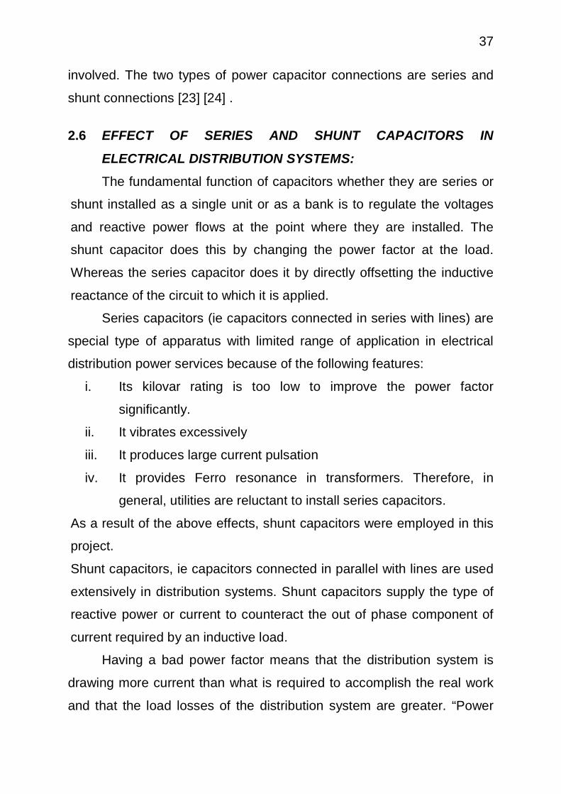
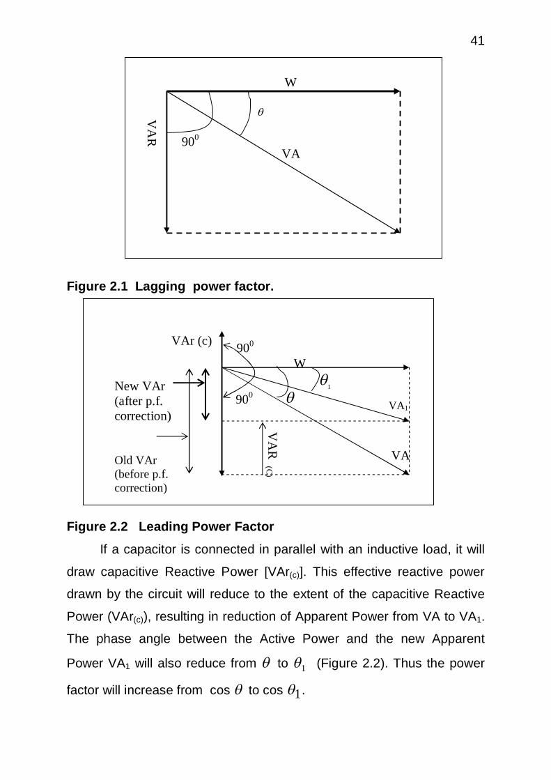
Figure 2.1 Lagging power factor.
Figure 2.2 Leading Power Factor
If a capacitor is connected in parallel with an inductive load, it will
draw capacitive Reactive Power [VAr(c)]. This effective reactive power
drawn by the circuit will reduce to the extent of the capacitive Reactive
Power (VAr(c)), resulting in reduction of Apparent Power from VA to VA1.
The phase angle between the Active Power and the new Apparent
Power VA1 will also reduce from to 1 (Figure 2.2). Thus the power
factor will increase from cos to cos 1 .
900
W
VA
VA
R
W
VA
R (C)
900 1
VA1
VA
900 VAr (c)
New VAr (after p.f. correction) Old VAr (before p.f. correction)

42
New p.f. = cos 1 = 1VA
W 2.9
By selecting a capacitor of an appropriate value, the power factor can be
corrected close to unity. In practice, the power factor is improved to fall
between 0.85 and 0.98
However there are two types of power factor correction, the
capacitive power factor correction and the active power factor correction.
2.7.1 CAPACITIVE POWER FACTOR CORRECTIONS
The capacitive power factor is corrected by addition of capacitors
to the distribution network in order to provide reactive compensation and
bring the power factor to an acceptable level. The capacitors are acting
as a storage device of reactive power which reduces the inductive
reactive power that the utility has to provide to the distribution network
and in turn improves the power factor of the system.
Electrical loads consuming alternating current power consume
both real power, which does useful work, and reactive power, which
dissipates no energy in the load and which returns to the source on each
alternating current cycle. The vector sum of real and reactive power is
the apparent power.
The ratio of real power to apparent power is the power factor, a
number between 0 and 1 inclusive. The presence of reactive power
causes the real power to be less than the apparent power, and so the
electric load has a power factor of less than unity [26].
The reactive power increases the current flowing between the
power source and the load, which increase the power losses through
distribution lines.
Power factor correction brings the power factor of an alternating
current (AC) power circuit closer to unity by supplying reactive power

43
opposite sign, adding capacitors or inductors which act to cancel the
inductive or capacitive effects of the load, respectively. For example, the
inductive effect of motor loads may be offset by locally connected
capacitors. Sometimes, when the power factor is leading due to
capacitive loading, inductors (also known as reactors in this context) are
used to correct the power factor. In the electricity industry, inductors are
said to consume reactive power and capacitors are said to supply it,
even though the reactive power is actually just moving back and forth
between each alternating current (AC) cycle.
2.7.2 THEORETICAL METHOD OF CAPACITIVE POWER FACTOR
CORRECTIONS:
As mentioned above, capacitive power factor is corrected by
addition of capacitor to the distribution network. The addition of
capacitors to the distribution network is the ideal way to provide reactive
compensation and bring the power factor to an acceptable level.
Capacitors can be added to the distribution network in the following
ways:
2.7.2.1 PERMANENTLY:
(i) Capacitors are connected directly to the lines and are in circuit all
the time.
Advantages: Minimum cost and easy installation
Disadvantages: Possibility of overcompensation is seen as a load
when all other loads are disconnected.
(ii). Parallel (shunt) Connection of Capacitors in Luminaires
Figure 2.3 is the most popular method of connection. The
capacitor is connected in parallel to the luminaires as shown in figures
2.3(a) and (b). The voltage rating of the capacitor is usually the same as
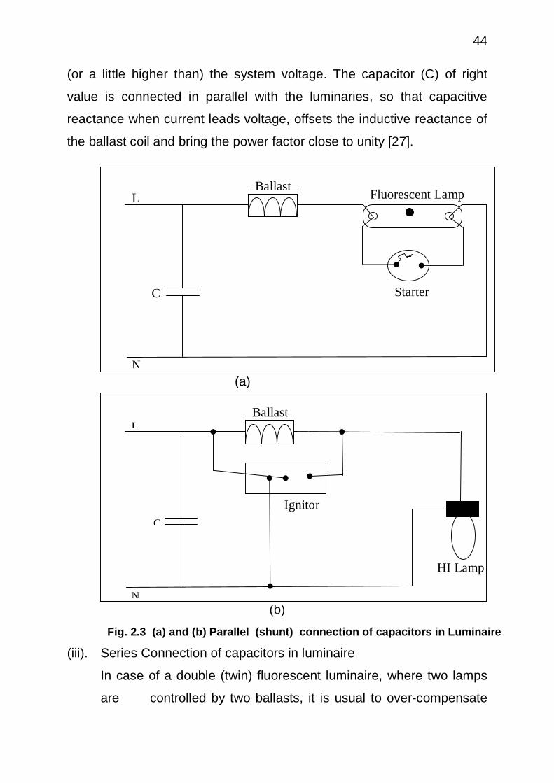
44
(or a little higher than) the system voltage. The capacitor (C) of right
value is connected in parallel with the luminaries, so that capacitive
reactance when current leads voltage, offsets the inductive reactance of
the ballast coil and bring the power factor close to unity [27].
(a)
(b)
(iii). Series Connection of capacitors in luminaire
In case of a double (twin) fluorescent luminaire, where two lamps
are controlled by two ballasts, it is usual to over-compensate
Ballast
N
L
C Ignitor
HI Lamp
Ballast
Starter
Fluorescent Lamp
N
L
C
Fig. 2.3 (a) and (b) Parallel (shunt) connection of capacitors in Luminaire

45
one ballast by connecting a capacitor in series with it, and to leave
the other ballast uncompensated. The leading power factor on the
first ballast, in conjunction with the lagging power factor of the
second ballast, brings the total power factor to near unity. The
scheme is shown in figure 2.4. The voltage rating of series
connected capacitors is much higher than the supply voltage and
must be correctly selected.
Figure 2.4 Series connection of capacitors in luminaries
Ballast
Starter
Fluorescent Lamp L
C
Ballast
Starter
Fluorescent Lamp
N
46
2.7.2.2 CONTROLLED:
Capacitors are switched on and off by contactors that are controlled by a
power factor regulator. (See figure 2.5)
Advantages: Accurate correction of power factor and easy installation.
Disadvantages: Requires more room.
Figure 2.5 Standard power factor Correction 2.7.2.3 AT THE MOTORS: [28] [29]
Capacitors are installed at the motors and connected either at the motor
leads or between the contactor and overload relay. (See figure 2.6)
Advantages: Maximum reduction of system losses.
Disadvantages: Economically not viable unless the motor load is mostly
constituted of large motors.
PFC Controller
Capacitor
Contactor
Motors
M M M

47
Figure 2.6 Capacitors connected to 3 phase motor.
2.7.3 METHODS OF IDENTIFYING POWER FACTORS IN DISTRIBUTION SYSTEMS:
Power factors in distribution systems are identified by applying
measurements on the system parameters. The preferred measurements
are kilowatts, kilovars and volts, from these the Kva and power factor
can be calculated. Voltage readings are especially desirable if automatic
capacitor control with a voltage – responsive master element is
contemplated. The types of meters and instruments available for power
factor are: Hook-on type ammeter, watt meter, voltmeter, varmeter and
power factor meter. The power factor can be obtained using the
following processes:
(i) Power factor meter can be used to measure the power factor in
a distribution system directly as a number between 0 and 1.
(ii) An oscilloscope can be used to compare the voltage and
current waveforms. By measuring the phase shift in degrees
between the current and voltage waveforms, the power factor
can be determined by taking the cosine of the phase shift.
(iii) The apparent power can be figured by taking a volt meter
reading in volts and multiply by an ammeter reading in
amperes. The wattmeter can be used to measure the true
Red Phase
Yellow Phase
Blue Phase
Induction motor

48
power. The power factor can therefore be determined by
dividing the true power (P) by the apparent power (S).
Power factor = SP 2.10
Using this value for power factor, a power triangle is drawn, and
from that determine the reactive power of the load (See figure 2.7
below).
Figure 2.7 Power triangle
To determine the unknown (reactive power) triangle quantity, we use the
Pythagorean theorem, given the length of the hypotenuse (Apparent
power) and the length of the adjacent side (true power).
Reactive power = 22 powerTruepowerApparent 2.11
If this load is an electric motor or most any other industrial alternating
current (AC) load, it will have a lagging (inductive) power factor, which
means that we will have to correct for it with a capacitor of appropriate
size, wired in parallel. If the amount of reactive power (Kvar) is known,
we can calculate the size of capacitor needed to counteract its effects
using the formula.
Reactive power (Q) ???
True power (P)
Apparent power (S)

49
Since this capacitor will be directly in parallel with the source (of
known voltage), we will use the power formula which starts from voltage
(E) and reactance (X) [28] [29].
Reactive power XEQ
2
Solving for capacitance of the capacitor ffx
C 21
2.15
2.7.4 CONVENIENT CALCULATION METHODS FOR CAPACITIVE
POWER- FACTOR (PF) IMPROVEMENT.
The two methods of improving power factor are by use of shunt
capacitors or synchronous motors. In this project shunt capacitors are
applied. The shunt capacitors are simply a capacitive reactance in shunt
or in parallel with the load or system and is fundamentally for power
factor improvement. The benefit of improved voltage level, released
system capacity, reduced system losses, and the reduction in power
bills, all stem from the improvement in power factor.
Power factor improvement is obtained by right- triangle
relationship.
Fig 2.8 Right-triangle relationship calculation in a.c. circuit.
fcXcceacCapacitive
QEX
XforSolving
21tanRe
2
2.12
2.13
2.14
P(KW)
S(KVA) Q(KVAR)

50
From the right-triangle relationship several simple and useful
mathematical expressions may be written:
cos = KVAKWPF 2.16
tanKW
KVAR 2.17
sin KVA
KVAR 2.18
Because the kilowatt component usually remains constant (the KVA and
KVAR components changes with power factor).
Therefore, equation 2.17 involving the kilowatt component is the most
convenient to use. This expression may be rewritten as:
KVAR = KW. tan 1 2.19
For example, assume that it is necessary to determine the capacitor
rating to improve the load power factor, we apply the following
equations:
KVAR at original PF = KW. tan 1 2.20
KVAR at improved pf = KW. tan 2 2.21
The angle is the phase angle between the voltage and current
waveforms. The reactive power is defined by
22 PSQ 2.22
Where S is the apparent power and P is the true power.
A capacitor of QKvar will compensate for the inductive Kvar and produce
Cos =1

51
It is not common practice to produce Cos =1 with capacitors because
this may result in overcompensation due to load changes and the
response time of the controller. Generally, public utilities specify a value
(Cos 2) to which the existing power factor (Cos 1) should be corrected.
The compensator ratings and various improved power factor values
could be determined as follows.
Q = P * (tan 1 -tan 2) [Var] 2.23
2
11
2
12
21
21
CorrectionFactor Power or factor power Improved
tantan
tantan
tantan
tantan*
CospfcPQ
pQ
PQ
pQ
Capacitors are used for Power Factor Correction because they offer the
following advantages.
(1) They have low temperature rise and negligible losses.
(2) They occupy little floor space
(3) They do not need special foundation [23], [33].
2.25
2.27
2.26
2.24
2.28

52
2.7.5 COMPENSATION THEORY FOR CAPACITIVE POWER
FACTOR CORRECTION.
(c)
Figure 2.9 Power Factor Correction (a – e)
(a) uncompensated system
(b) corresponding phasor
(c) power diagram
(d) compensated system
(e) corresponding phasor diagram [25], [30]
Consider the single phase system shown in fig 2.9. (a) Having a
load of admittance YL = GL+jBL which is supplied from a voltage V.
When V is taken to be reference phasor, the resulting load current,
IL= VYL = V (GL + jBL) = VGL + jVBL = IR + jIx 2.29
Hence, it is apparent that the load current consists of a real component,
IR, which is in phase with V, and a reactive component, Ix, which is in
PL
QL SL
øL
YL = GL + jBL Load
IL
Is V
(a)
V
IL IX
IC
IR = IL1 = Is
Compensator Yc = jBc
Load
Ic
I1L
V
(d)
IL
YL = GL + jBL
Supply System IS
v IR
IL = Is Ix (b)
øL
Ix1 = Ix + Ic = 0
(e)

53
phase quadrature with V. The phasor diagram for an inductive load,
which is the most common case, is given in Fig 2.9. (b). In this case, the
reactive current, Ix , is negative and load current, IL, is said to be
lagging the voltage, V. The angle between the voltage and the load
current is L .
For the system shown in figure 2.9 (a), the apparent power, SL, supplied
to the load is given.
SL = 1LVI = V2GL – JV2BL = PL + QL 2.30
Hence, it is clear that the apparent power has a real component,
PL and a reactive component, QL. The real power, or active power as it is
sometimes referred to, is the power which is capable of being converted
into useful forms of energy such as heat, light and mechanical work.
The relationship between the real, reactive and apparent powers is
shown in figure 2.9 (c). By convention, BL is negative and QL is negative
for inductive loads.
For the system shown in figure 2.9 (a), the current, IS, supplied by
the power system is equal to the current consumed by the load ie IS = IL.
Furthermore, from figure 2.9 (b), it is clear that the current supplied by
the power system is larger than that which is necessary to supply only
the real power required by the load by the factor. lLR
L
Cos1
11
2.31
In addition, from figure 2.9 (c) the ratio of the active power to the
apparent power is given by:
Cos L = L
L
SP
2.32

54
Hence, the quantity, Cos L , is commonly referred to as the power
factor, as it represents the fraction of the apparent power which can be
converted into useful forms of energy.
As a result of the reactive power required by the load being
supplied from the supply bus, the joule losses in the distribution cables
are increased from that when only the real power required by the load is
supplied from the supply bus by the factor LCos 2
1 . Consequently, it is
desirable to keep the power factor near to unity. For poor power factor
loads, Cos L < 0.95, compensation is generally employed in order to
improve the power factor. Compensation for this purpose is known as
power factor correction. Power factor correction is performed by locally
generating the reactive power required by the load, instead of supplying
it through the distribution lines from the power system. In this way, the
losses are reduced, and the entire distribution system operates more
efficiently.
The method of power factor correction just outlined may be
accomplished by connecting a compensator having a purely reactive
admittance, Yc = -jBL, in parallel with the load, as shown figure 2.9(d).
As a result of this compensation, the current supplied by the power
system becomes:
2.33
Where Ic is the current drawn by the compensator and 1,LI is the
total current drawn by the load compensator combination. In addition,
the apparent power Ss supplied by the power system is
2.34
RLLLLLLS IVGjBVjBGVIcIII 1
LLLLLILS PGVjBVjBGVVVIS 2

55
From equation 2.33 it is apparent that the supply current of the
compensated system is now in phase with V, and has the lowest
possible magnitude which is capable of completely supplying only the
active power requirement of the load. The phasor diagram for the
compensated system is given in figure 2.9 (e).
For total compensation it is clear from figure 2.9 (c) that the
reactive power rating of the compensator is related to the rated power of
the load by
LLL PQ tan 2.35
LL
L PQ tan 2.36
and to be rated apparent power by
LLL COSSQ 21 2.37
LL
L COSSQ 21 2.38
LL
L SinSQ 2.39
Where Q is the reactive power, P is the real power, S is the apparent
power.
The compensator rating per unit apparent power and per unit real power
for complete compensation for various power factors are shown in
table 2.1.

56
Table 2.1 Rated reactive power of the compensator required for full
compensation per unit rated apparent power of the load and per unit real
power of the load for various power factors and the corresponding factor
by which the losses are increased.
Power
factor Angle L
L
L
SQ
L
L
PQ
LCOS 2
1
1.0 0 0 0 1.00
0.95 18.19 0.312 0.329 1.11
0.90 25.84 0.436 0.484 1.23
0.85 31.79 0.527 0.620 1.38
0.80 36.87 0.600 0.750 1.56
0.75 41.41 0.661 0.882 1.78
0.70 45.57 0.714 1.020 2.04
0.65 49.46 0.760 1.169 2.37
0.60 53.13 0.800 1.333 2.78
Source: Reference [25]
It is also possible to partially compensate the load. The degree of
composition which is required for a particular system depends on an
economic trade-off between the capital cost of the compensator, which is
proportional to its rating, and the cost of the power and energy losses
over a period of time associated with the supplying the reactive power
required by the load through the distribution system.
Consider for example, an uncompensated load having a power
factor of 0.90, from table 2.1 it is clear that in order to completely correct
the power factor of this load a compensator with a rating of 0.436 per
unit apparent power is required, while to correct the power factor to be
no worse than 0.95 would only require a compensator with a rating of

57
0.312 per unit apparent power, this would translate into considerable
saving in the cost of the compensator employed.
Real distribution system, however, may contain hundreds of buses. In
this case, compensation at one bus will effect the level of compensation
required at another bus. In addition, in order for a compensation scheme
to be practical it must be economical. Hence, not every bus will require
compensation. As a consequence, it is necessary to first determine
which buses require compensation and which buses do not. This step is
known as placement problem.
The placement problem involves planning and consists of
determining optical location, size and number of compensators that are
required for a distribution system, taking into account the cost of the
compensators, the savings from energy and power loss reduction. The
placement problem is a means of improving the performance of the
distribution system and can be performed off-line.
The capacitor sub-problems mentioned above were solved in this
project as follows:
i. Heuristic method is used to solve capacitor location sub-problem.
ii. The size subproblem of capacitors in kilovars is determine by
calculating the rate of return and actual naira savings for various
final power factor values.
iii. Number of capacitors required in the system have no specific
formular, rather it could be found using the iterative process of
finding the savings.
The installation of shunt power capacitors can reduce current flow
through the system from the point of the capacitor installation back to the
generation.
58
Since power losses are directly proportional to the square of the
current, a reduction of current flow results in a much greater reduction of
power losses. Capacitors are often installed as close to the load as
possible for this reason.
The quality of service of a power system depends on the correct
voltage level being consistently available to the customer. In order to
ensure this, reactive power compensation is often needed on the
distribution system.
Compensation may be performed for various reasons and by
various methods. Compensation is performed for the following
reasons [30]:
i. It increases system capacity.
ii. It improves voltage profile.
iii. It reduces billing charges.
iv. It reduces system power losses.
Increased System Capacity: Increased system capacity is often the
most important benefit justifying the addition of shunt power capacitors
on a distribution system. This is particularly significant when loads
supplied by the system are increased rapidly. When capacitors are in
operation in a distribution system, they deliver kilovars, furnishing
magnetizing current for transformers, therefore reducing the current from
the power supply. Less current means less kilovaltampere (KVA) or load
on transformers and main branch, feeder circuits. For a given power, the
higher the power factor, the lesser must be the size of the transformer to
distribute the power and the lesser must be the cross-sectional area of
the conductor to distribute it.
This means that capacitors can be used to reduce overloading of
existing facilities or if the equipment is not overloaded, capacitors can
permit additional load to be added.

59
Therefore, the addition of shunt power capacitors reduces the
kilovoltampere loading on the system, thereby releasing capacity that
can then be used to supply future load increase. The optimum
economical power factor for a system, with regard to released capacity
only, can be estimated by use of the following formula:
2
1
i
i
SCPf 2.40
Where:
Ci is the cost per kilovar of capacitor bank
Si is the cost per kilovoltamperes of system equipment.
Pf is the optimum power factor.
The formula compares the cost of capacitor banks to the cost of
transformers as alternative means of providing increased system
capacity.
Improved System Voltage Profile: Applying capacitors to a system will
result in a voltage rise in the system from the point of installation back to
the generation. In a system with lagging power factor, this occurs
because capacitors may reduce the amount of reactive current being
carried in the system, therefore, reducing the amount of resistive and
reactive voltage drop in the system. There are a number of formulae that
can be used to estimate the voltage rise that capacitors will produce. A
commonly used one is as follows:
210
varKV
XKV L 2.41
Where:
V is the percent voltage rise at the point of the capacitor installation.
KV is the system line to line voltage without capacitor in service [30]
varK is the three phase kilovar rating of the capacitor bank.

60
LK is the inductive reactance of the system at the point of the capacitor
installation, in ohms. Capacitor banks are typically installed at
distribution buses and directly on customer delivery buses to provide
voltage support to smaller areas and to individual customers. Capacitor
banks installed on distribution lines support voltage along the entire
length of line.
Reduced Billing charges: A number of utilities use some form of
kilovaltampere billing for their large customers (e.g; utilities and large
industrial customers). Since the application of shunt power capacitors
can result in a reduced kilovaltampere loading, this can result in reduced
billing charges.
The kilovaltampere billing charge may be calculated in many ways,
including the following:
(i) A charge per kilowatt demand multiplied by a factor that increases
with decreasing power factor.
(ii) A fixed charge per peak kilovaltampere
Reduced System Power Losses: On some distribution systems, a
significant reduction in losses may be achieved by the installation of
shunt power capacitors. The installation of shunt power capacitors can
reduce current flow through the system from the point of the capacitor
installation back to the generation. Since power loses are directly
proportional to the square of the current, a reduction of current flow
results in a much greater reduction of power losses. Capacitors are often
installed as close to the load as possible for this reason. Reactive power
compensation can be achieved by connecting capacitors permanently to
the lines [30].
The addition of shunt power capacitors reduced kilovar current.
When the kilovar current in a circuit is reduced, the total current is
reduced, if the kilowatt current does not change as is usually the case;

61
the power factor will improve as kilovar current is reduced. It is a well
known fact that shunt power capacitors are the most economical source
to meet the reactive power requirements of inductive load and
distribution lines operating at a lagging power factor. When reactive
power is provided only by power plants, such system components (ie
generators, transformers, distribution lines etc) has to be increased in
size accordingly. Capacitors can mitigate these conditions by decreasing
the reactive power demand back to the generators. Line currents are
reduced from capacitor locations back to generation equipment. As a
result, losses and loadings are reduced in distribution lines.
Reactive Power compensation or power factor correction is performed
by the following methods:
(i) Individual Power Factor Correction:
To individually correct the power factor of a multiple load, a
suitably sized capacitor is connected to each element of the total
load.
(ii) Group Power Factor Correction
Group power factor correction is achieved by connecting one
capacitor to a number of different loads usually sharing the same
duty cycle.
A shared duty cycle prevents the use of too much capacitance and
avoids over correction of the power factor.
(iii) Centralized Automatic Power Factor Correction:
This involves the connection of number of capacitors, usually to
the supply distribution point. The capacitors are controlled by a
microprocessor based relay which monitors the reactive power
demand on the supply. The relay connects and/or disconnects the
capacitors to automatically compensate for the reactive power on
the system.

62
Choosing the most appropriate type and level of compensation
necessarily is important, as overcompensation can be as harmful to the
system as under compensation. Once the appropriate type of
compensation has been determined, a method of controlling the
compensators under the varying load conditions of the system must be
formulated.
2.7.6 POWER LOSS REDUCTION USING CAPACITOR
Electrical distribution power losses can be reduced using
capacitors as shown in figure 2.10.
Without capacitor installed (i.e, the off state or when the switch, S,
is open), the current flowing in the line, Ia, is equal to the current flowing
in the load, Iload. Also, depending on the power factor, the current Ia is
composed of real and imaginary part, Iax + jIay. However, what
contributes in the real power losses is the magnitude of the current, that
is, power loss in the line is equal to the resistance of the line multiplied
by the square of the magnitude of the current. [31].
But, with capacitor installed (ie the On-state or when the switch, S,
is closed), the capacitor supplies reactive power (Kvar). This amount of
Kvar injects current that is, ideally, purely imaginary, thus reducing the
Figure 2.10 Capacitive Power Loss Reduction
Ia
(Ic)
(S)
I load
(R) (L)
(C)
2 1 Resistor Inductor
Switch
Capacitor
Capacitor Current

63
amount of imaginary component of the power that flow in the line. This
reduction of imaginary component of current that flow in the line also:
i. reduces the magnitude of current that flows,
ii. reduces the amount of voltage drop
iii. reduces the phase angle difference between the voltage and the
current, thereby improving the power factor, and most importantly,
iv. reduces the 12R power losses in the distribution line.
Capacitor placement in a distribution system can reduce power
losses in electrical distribution feeder. In addition to loss reduction, there
are also other benefits like, increase in receiving of voltage profile,
increase of equipment capacity, etc. However, if the placement of
capacitors is not optimized, it can cause either,
1. minimal loss reduction or
2. incure additional loss due to KVAR overcompensation.
2.7.7 CONSIDERATION OF HARMONICS WHEN APPLYING
CAPACITORS.
The level of harmonic voltage and current on distribution systems
are becoming a serious problem. Some of the problems caused by
harmonics are: capacitor bank failure from dielectric breakdown or
reactive power overload, over voltages and excess currents on the
system from resonance to harmonic voltages or currents on the network,
dielectric instability of insulated cables resulting from harmonic
overvoltages on the system etc. These effects depend on the harmonics
source (e.g network nonlinearities from loads such as rectifiers,
inverters, welders, arc furnace, voltage controllers, frequency converter
etc. The presence of harmonics causes the distortion of the voltage or
current waves. [32]

64
The impact of harmonics on distribution transformers are
numerous. For example, voltage harmonics result in increased iron
losses, current harmonics result in increased copper losses and stray
flux losses. The losses may in turn cause the distribution transformer to
be overheated and cause more power losses.
Therefore, system harmonics should be considered when applying
power factor correction capacitors. Although capacitors do not generate
harmonics, under certain conditions they can amplify existing harmonics.
Harmonics are generated when non-linear loads are applied to power
systems. These non-linear loads include: adjustable speed drives,
programmable controllers, induction furnaces, computers, and
uninterruptible power supplies. Capacitors can be used successfully with
non-linear loads when harmonic resonant conditions are avoided.
To minimize the occurrence of harmonic resonance, the resonant
harmonic of the system including the capacitor should be estimated. The
resonant frequency can be calculated by:
KVARKVAsch
Where: h = calculated system harmonic
KVAsc = short circuit power of the system
KVAR = rating of the capacitor. Harmonic values of 5,7,11, and 13
should be avoided as they correspond to the characteristic harmonics of
non-linear loads. The harmonic value of 3 should also be avoided as it
coincides with harmonics produced during transformer energization
and/or operation of the transformer above rated voltage. Once identified,
the resonant harmonics can be avoided in several ways.
i. Change the applied KVAR to avoid unwanted harmonics.
Although this is the least way to avoid resonant harmonics, it is not
always successful because typically some portion of the applied
2.42

65
KVAR is switched on and off as load conditions require. The
calculation of system harmonics should be repeated for each level
of compensation. Adjusting the size of the capacitor(s) may be
necessary to avoid the harmonic values.
ii. Add harmonic filters.
In order to filter harmonics at a specific site, tuned harmonic filters
can be applied. A capacitor is connected in series with an inductor
such that the resonant frequency of the filter equals the harmonic
to be eliminated. Turned filters should never be applied without a
detailed analysis of the system. The currents expected to flow in
the filter are difficult to predict and are complex function for the
system characteristics.
Figure 2.11 Addition to Harmonic Filters
iii. Add Blocking Inductors
Inductors added to the line feeding the capacitor can be sized to
block higher than 4th harmonic currents. This method protects the
capacitor from the harmonics but does not eliminate the harmonics
from the system. A system study is required to determine correct
ratings for the capacitor and inductors.
Power Factor Correction Capacitor
Tuned Filter
Harmonic Generator

66
2.7.8 CARDINAL RULES FOR APPLICATION OF CAPACITOR
BANKS IN A DISTRIBUTION SYSTEMS:
a. The cumulative data gathered for the whole utility industry indicate
that approximately 60 percent of the capacitors is applied to the
feeders, 30 percent to the substation buses and the remaining 10
percent to the transmission system.
b. There is only one location for each size of capacitor bank that will
produce maximum loss reduction.
c. Whenever possible, capacitors should be located at or near the
load on systems in order to obtain minimum cost and maximum
benefits. Maximum benefits are obtained when they are located at
the load.
d. Capacitors are also installed or located at the sensitive nodes
especially when the system is having concentrated load.
Concentrated load means that the load is centered at the node. In
this project the capacitors are installed at the sensitive nodes
because the distribution system is a concentrated load system.
e. It is usual to have the capacitors in several banks so that individual
banks can be switch in or out of circuit either automatically or
manually as the factory load changes. [33]
f. The best way to determine the capacitor kilovars to use is to
calculate the rate of return and actual naira savings for various
final power factor values.
g. In actual practice, it is generally not necessary or economical to
improve the power factor to 100 percent, capacitors are used to
supply part of the load kilovar requirements and the supply system
provides the remainder.
h. All capacitor banks should be equipped with a means to
disconnect them from the electric system.

67
Reasons for the application of shunt capacitor units in the distribution
system are because, it:
(i) Provides low temperature rise and negligible losses.
(ii) Occupy little floor space.
(iii) Needs no special foundation.
(iv) Increases voltage level at the load.
(v) Improves voltage regulation if the capacitor units are properly
switched
(vi) Reduces I2R power loss in the system because of reduction in
current.
(vii) Reduces I2X kVAR loss in the system because of reduction in
current.
(viii) Increases power factor of the distribution systems.
(ix) Releases the distribution systems capacity for additional load
growth.
2.8 ACTIVE POWER FACTOR CORRECTION.
An active power factor correction (Active PFC) is a power
electronic system that controls the amount of power drawn by load in
order to obtain a power factor close as possible to unity. In most
applications, the active power corrector controls the input current of the
load so that the current waveform is proportional to the main voltage
wave form [34].
One type of active power factor correctors is the boost converter:
Active power factor corrections can be single-staged or multi-stage.
In the case of a switched-mode power supply (SMPS), a boost converter
is inserted between the bridge rectifier and the main input capacitors.
The boost converter attempts to maintain a constant DC bus voltage on
its output while drawing a current that is always in phase with and at the

68
same frequency, as the line voltage. Another switchmode converter
inside the power supply produces the desired output voltage from the
DC bus. This approach requires additional semiconductor switches and
control electronics but permit cheaper and smaller passive components.
It is frequently used in practice. Switched-mode power supply with active
power factor correction can achieve power factor of about 0.99.
The boost converter operating in a continuous current mode (ie the value
of the inductor at the input is calculated such that it conducts
continuously throughout the switching cycle) applies the smallest amount
of high frequency current to the input capacitor Ci (see figure 2.12). It is
the only topology which allows the noise across the input capacitor to be
reduced, which is the major factor defining the size and cost of the filter.
Additionally, the boost inductor stores only a part of the transferred
energy (because the mains still supplies energy during the inductor
demagnetization) and so the inductor required is smaller in comparison
with the other topologies. The boost topology therefore leads to the
cheapest power factor corrector solution but does not provide either in
rush current or short circuit protection. The basic topology of a boost
power factor corrector is as shown in figure 2.12 [35].

69
Figure 2.12: Basic topology of a Boost PFC
Source: Reference [35]
NTC
Cs
FUSE
LS
Ci
Lb
Cd TURBOSWITCH
Cout
RS
CONTROL IC
T
D

70 2.8.1 BOOST CIRCUIT PARAMETER OPTIMIZATION
Figure 2.12 shows the general topology of a Boost Power Factor
Correction (BPFC)
Its optimization requires careful adjustment of the following parameters:-
(a) The value of the input capacitor C1.
(b) The current ripple in boost inductor Lb
(c) The parastic capacitances of the boost inductor and the power
semiconductors, including those associated with the heat sink.
(d) The operating frequency and frequency modulation techniques.
2.8.2 VALUE OF THE INPUT CAPACITOR C1.
The noise across the input capacitor is proportional to the current
ripple and inversely proportional to the capacitor value.
2.8.3 CURRENT RIPPLE IN THE BOOST INDUCTOR.
The input ripple ( i is a function of the input voltage (Vi), output
voltage (Vout), inductor value (Lb) and switching frequency (FS), and can
be expressed as
VoutLF
ViViVoutibs ..
. 2.43
Assuming the typical values Vi = 300V, Vout = 400V
FS = 70KHz and Lb = 1mH
If the system is operating in continuous mode, a typical value of i may be 1A.
If the system operates in discontinuous mode with Lb = H150 , i
might be 7A. Using a continuous mode requires an inductance value
about ten times that need when operating in discontinuous mode,
however, the low value of current ripple means that a cheaper and
efficient iron powder core can be used.

71 When operating with ripple current larger than around 1A, the
larger dtdi leads to the occurrence of skin effects and large eddy
currents in an iron powder core, meaning that operation in discontinuous
mode requires a more expensive ferrite core.
So, a cheaper system is achieved controlling a small current ripple
by operating in continuous mode, despite the large inductor value.
For any design over 100W, the preferable type of Power Factor
Correction is Active Power Factor Correction (Active PFC) since it
provides a lighter and more efficient power factor control. Active PFC is
comprised of a switching regulator operating at a high switching
frequency, being able to generate a theoretical power factor of over
95%. Active Power Factor Correction automatically corrects for AC input
voltage, and is capable of a wide range of input voltage. One
disadvantage of Active PFC is the extra cost resulting from the additional
complexity required in its implementation [36].
Figure 2.13: Basic Active Power Factor Correction Circuit
Figure 2.13 above depicts the basic elements of an active power
factor correction circuit. The control circuit measures both the input
voltage (pin 2 on the controller) as well as the current (RS, pin 3 and 11
on the controller) and adjust the switching time and duty cycle to present
an in phase voltage and current load to the input. The Power Factor
INPUT
BRIDGE RI LOAD
LI DI
CONTROL CIRCUIT
2 19
11 3
15 Q1
C1
RS

72 Correction (PFC) works by inducing a current in the inductor (L1) and
causing the current to track the input voltage. The control circuit senses
both the input voltage and the current flowing through the circuit. By
controlling the on time in the switch (Q1) that places L1 across the output
of the rectifier, the current in the coil increases as the input voltage
increases. The switch is turned off periodically and the voltage at the
drain end rises until the current in the inductor voltage achieves the
charge level. Usually, this level is set to several volts higher than the
bridge rectifier peak output voltage.
The active PFC shown above is in the form of a boost regulator
and as a result the voltage appearing across the load (R1) must be
greater than the highest value of the peak voltage appearing at the input.
Using an active PFC circuit, any input voltage ranging from 87 to
266V (RMS) can be accommodated and power factors 98.0 can be
achieved with relative ease. Example of active P.F.C is the Active Power Factor Correction
Technique for Three-Phase Diode Rectifiers shown in figure 2.14.
2.8.4 PRINCIPLES OF OPERATION OF ACTIVE POWER FACTOR
CORRECTION TECHNIQUE FOR THREE-PHASE DIODE RECTIFIERS
The proposed three phase ac to dc converter (fig. 2.14) consists of
two main power conversion stages. The first stage is a three phase ac to
dc rectifier consisting of an input filter, a boost inductor, a three phase
diode rectifier, an active power factor correction stage, and a dc link filter
capacitor. The second stage can be modeled as any type of load
requiring a regulated or unregulated dc bus such as general purpose
single phase or three phase inverters or dc to dc converters with high
frequency isolation. The active waveshaping of the input current

73 waveform is obtained through the use of the three boost chopper
components Lia, Qb and Db, as shown in fig. 2.15 [37]
RC
SOURCE
INPUT
FILTER
BOOST
INDUCTOR
RECTIFIER ACTIVE P.F.
CORRECTION
DC
FILTER
CAPACITOR
LOAD
(a)
AC
SOURCE
AND
INPUT
FILTER
BOOST
INDUCTOR
RECTIFIER ACTIVE P.F.
CORRECTION
DC FILTER
CAPACITOR
LOAD
(b) Fig. 2.14 (a) Proposed three-phase ac to dc converter. (b) Single-phase equivalent circuit of (a)
v d
Van
Vbn
Vcn
Ii3 Li3
Ii2 Li2
Ii1
Li1 Lia Iia
3CiC
3Cia
Lib Iib
3Cib
Lic
Iic
n
Idc Db Db Ii
Ib2
Cd
QI g
f e
Van Vda Qb Cd
Db Iba Ida Iia
34V
Vda
Li1 Lia
Iia
Cia
Ii1
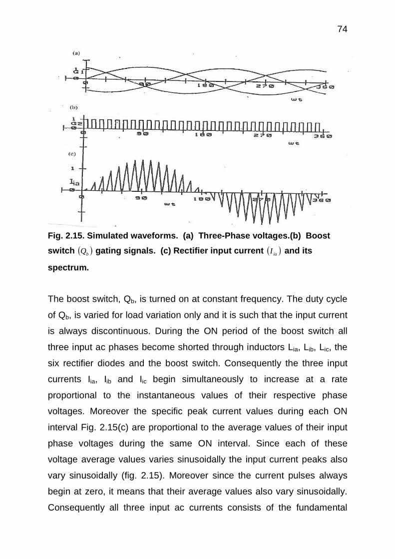
74
Fig. 2.15. Simulated waveforms. (a) Three-Phase voltages.(b) Boost
switch bQ gating signals. (c) Rectifier input current iaI and its
spectrum.
The boost switch, Qb, is turned on at constant frequency. The duty cycle
of Qb, is varied for load variation only and it is such that the input current
is always discontinuous. During the ON period of the boost switch all
three input ac phases become shorted through inductors Lia, Lib, Lic, the
six rectifier diodes and the boost switch. Consequently the three input
currents Iia, Iib and Iic begin simultaneously to increase at a rate
proportional to the instantaneous values of their respective phase
voltages. Moreover the specific peak current values during each ON
interval Fig. 2.15(c) are proportional to the average values of their input
phase voltages during the same ON interval. Since each of these
voltage average values varies sinusoidally the input current peaks also
vary sinusoidally (fig. 2.15). Moreover since the current pulses always
begin at zero, it means that their average values also vary sinusoidally.
Consequently all three input ac currents consists of the fundamental

75 (60Hz) component and a band of high frequency unwanted components
centered around the switching frequency (fb) of the boost switch. Since
this frequency (fb) can be in the order of several tens of KHZ, filtering out
of the unwanted input current harmonics becomes a relatively easy task.
From fig. 2.15 it is also seen that input power control (or output voltage
regulation) can be achieved through pulse with modulation of the boost
switch ON interval at constant frequency (fb).
Incidently fb can be easily locked to the main 60Hz frequency to
avoid beat frequency effects in the input currents.
Finally, under the operating conditions described here the
displacement input power factor (cos 1 ) before filtering is unity.
Consequently, the overall input power factor (before filtering) becomes
equal to the harmonic input power factor and it is given by:
Power factor =
1
2.
.
2
2
n
nia
Iia
L
L 2.44
Where
Lia.n is the fourier component of the nth harmonic component of
current Iia.
cos 1 is the displacement factor .
It is noted that the current harmonics associated with this power factor
can be suppressed by a relatively small input capacitor (Cia) and inductor
(Li1) because of their high frequencies.
Therefore the overall input power factor after filtering (ie…at the ac
source) is very close to unity.

76 2.9 PROPERTIES OF CAPACITIVE AND ACTIVE POWER FACTOR
CORRECTIONS
Capacitive power factor correction Active power factor correction
Features Inductors, capacitors and
resistors
Complete solutions including all components for PFC-BOOST topology such as Boost converter, Bridge rectifier etc. Output voltage is greater than Input voltage (Vo > Vi), Efficiency 95%, Power factor 99%.
Advantages It improves power factor over
98%.
It releases system capacity. It reduces system power losses. It reduces billing charges. It improves voltage profile. It has no current or voltage surge. It has no inrush current, therefore transformers are not subjected to short circuit currents and hence the life of the transformer increases. Compensation at extremely low voltage is possible. As there is no moving part involved, maintenance cost is negligible. It is not complex and bulky. It occupies little floor space It is more practicality
It is less expensive and easy to
install
It provides a steady power system frequency. It generates power factor over 99%. It reduces total harmonics. It automatically correct for alternating current (AC) input voltage and it is capable of a full range of input voltage.
Disadvantages Switching the capacitors into or out of the circuit causes harmonics. It may be affected when environmental vibration occurs. It requires that AC input voltage be set normally.
Possibility of overcompensation, is seen as a load when all other loads are disconnected.
It is more complex method of power factor correction. It is more expensive to produce an active power factor correction power supply. It does not provide either in rush current or short circuit protection. Therefore, high inrush current increases the possibility of capacitor, exploding and catching fire, because there is excessive pressure generated inside the capacitor unit, so life of capacitor progressively deteriorates. Compensation at low voltage is not possible, resulting in wear and tear of mechanical parts. It has large switching surges even as high as 200 times of rated capacitor current.

77
Capacitive power factor correction Active power factor correction
Repeated and momentary short circuit due to capacitor switching will have an impact on the life of the transformers. The contactor chatter at low voltages resulting in very high inrush current.
Limitations It is limited to 180o out of phase. The allowable overload limits of capacitors based on IEEE std 18-2002 are as follows: (i) 110% of rated rms voltage (ii) 120% of rated peak voltage,
including harmonics (iii) 135% of rated kvar
It is limited to 180o in phase. According to regulatory requirement, the maximum amplitude of line frequency harmonic is limited to 39th harmonic. For equipment like personal computers, televisions and monitors, the harmonic amplitudes are proportional to the input power of the device.
Applications It is applicable in high voltage distribution and transmission systems. It is used for AC supplies only.
It is welcome to supply power for personal computers, telecommunications battery powered systems, it is used for supply of dc powers.
Formular for
power factor.
Power factor =
22 KVARKW
KW
Power factor = 2
100%1
1
THD
Source: Reference [26], [38]
2.10 COMPARISON OF CAPACITIVE AND ACTIVE POWER FACTOR
CORRECTIONS
CAPACITIVE POWER FACTOR CORRECTION
ACTIVE POWER FACTOR CORRECTIONS
* It improves power factor aver 98% * It improves power factor aver 99% * It reduces resonant harmonics * It reduces total harmonics * The is no current or voltage surge * Large switching surges even as high as 200
times of a rated capacitor current * There is no inrush current, transformers are never subjected to short circuit currents and hence the life of the transformers increases
* Repeated and momentary short circuit due to capacitor switching will have an impact on the life of the transformers.
* Compensation at extremely low voltage is possible
* Compensation at low voltage is not possible, resulting in wear and tear of mechanical parts.
* The point of capacitor switching is controlled and increases the life of the capacitor and switching unit.
* High inrush current increases the possibility of capacitors exploding and catching fire because there is excessive pressure generated inside the capacitor unit, so life of capacitor progressively deteriorates.

78
CAPACITIVE POWER FACTOR CORRECTION
ACTIVE POWER FACTOR CORRECTIONS
* It is not complex and bulky. * It is a complex and bulky circuit. * It occupies very little space and has low weight, so that it can be mounted on distribution lines without pulling the poles.
* It occupies a very large space and it has high weight such that it cannot be mounted on distribution lines to avoid distortion of cables and poles
* It is not expensive to produce capacitive (reactive) power factor correction.
* It is very expensive to produce active power factor correction power supply.
* It is limited to 180o out of phase of voltage and current waveforms.
* It is limited to 180o in phase of voltage and current waveforms.
* It is more practicability * It is less practicality.
Active power factor produces power factor correction, close to
unity as well as capacitive power factor correction but capacitive power
factor correction was chosen because it is less expensive, not complex,
very easy to implement, lower weight and occupies very little space than
active power factor correction component. [26], [38].

79
CHAPTER THREE
LOAD FLOW ANALYSIS AND SYSTEM MODELLING
3.1 SYSTEM MODELING
In this project, the distribution system is assumed to be a balanced
three phase system, and hence a single phase representation can be
used. The control devices consists of shunt capacitors which are
assumed to be already placed optimally on the system. The distribution
system is modeled using a equivalent representation.
Shunt capacitors are frequently used on distribution system for power
factor correction and voltage support. For purpose of modeling,
capacitors are treated as constant shunt admittance element on a per-
phase basis.
In this chapter the mathematical analysis were carried as follows:
(i) Load flows
(ii) Load variation with time
(iii) Derivation of power loss reduction formulae or equations
(iv) Derivation of economical power factor
3.2 LOAD FLOWS.
The load flow is a computer algorithm that displays the kilowatt
(KW) and Kilovolt-ampere reactive (Kvar) loading of distribution lines and
transformers after an iterative process of solving for node voltages. It is
like using an ammeter and voltmeter to determine the junction voltages
and current on the resistors of figure 3.1. But instead of amperes, line
flows are in KW and Kvar. Instead of V = 126 volts from dry cells, the
source feeding the circuit is in KW and Kvar. All other units are in per
unit. Most chosen base MVA is 100.
Load flow analysis is used to determine the apparent power and
voltages at each bus in the distribution system under steady state
conditions. While there are several methods for performing load flow

80 analysis the Gauss-Seidel technique and the Newton-Raphson
techniques are perhaps the most common. Both methods can be carried
out very quickly using modern computers, however, the Gauss-Seidel
method is preferred for distribution systems as the low X/R ratios typical
of distribution systems often leads to ill-conditioned Jacobian matrices
which can cause the Newton –Raphson method to fail to converge. As
well, the Gauss- Seidel technique has the following advantages [25],
[39].
(i) It is relatively insensitive to the initial voltage estimates,
(ii) It has reasonably small memory requirements, and
(iii) It is simple to implement in a computer program.
Every possible solution in the control problem requires a load flow
to be performed so that its merits can be assessed. As a result, for a
large distribution system, even with the use of a fast computer, the time
required to complete a load flow to evaluate every solution would be
prohibitive. This is the main reason for not performing an exhaustive
search.
While the use of an optimization technique such as genetic
algorithm does reduce the number of times that the load flow analysis
must be performed, the load flow still consume most of the processing
time required by the optimization technique. It is important therefore to
examine the issue using the equivalent representation as shown in
figure 3.3.
Types of variable used:
(i) Uncontrollable or disturbance variable P,Q (load) are beyond
control since they are dictated by the customer.
(ii) State or dependent variable, voltage (V) magnitude and angle
(theta) are computed based on the other two variables.

81 Table 3.1 Classification Of Load Flow Busses
Type Known variables Unknown variables
(i) Sl, Swing or Slack or
Reference bus
V, theta P,Q Losses
(ii) P Q, load bus P, Q V, theta
Where:
V = voltage magnitude
Theta = voltage angle
P, Q = KW, KVAR load.
3.3 NODE EQUATIONS
Let us derive the nodal equation using a simple electrical circuit
shown in figure 3.1.
Figure 3.1 simple electric circuit
The junctions formed when two or more elements (R, L, C, etc) are
connected are called nodes. One of them is designated as reference. By
applying kirchoff’s current law, we can derive the nodal equations. The
sum of the current entering the node equals the sum of the currents
leaving the node. When making the current equation for node i, we
assume node i to be of a higher potential than node j. In node 1 for
node node Node
1
+ 1
VO1 126 volts
2
Node 4
2 1 O
72 volts
V02
2 2
5
3

82 example, the left side is the current source and the right side is [V (1) – V
(2)] r (1, 2). [39]
Here node 1 is of a higher potential than node 2, we do this to all nodes
except the reference. If there is no current source, put zero on the left
side, as in node 3. Therefore:
3,1
31
2,1
21
,
,
rVV
rVV
rV
IO
IO
node 1
2,1
12
3,2
32
2,0
2,
rVV
rVV
rVO
node 2
3,2
23
3,1
13
3,0
3
3,0
3,
rVV
rVV
rV
rVO
node 3
Equation 3.1 can be written as:
33,1
22,1
13,12,1
11111 V
rV
rV
rrI
33,2
22,13,2
12,1
21111 V
rV
rrV
rI
3.2
33,23,13,0
23,23,1
311111 V
rrrV
rV
rI I
Rearranging equation (3.2) in matrix form we get:
3
2
1
3,23,13,03,23,1
3,22,13,22,1
3,12,13,12,1
3
2
1
11111
1111
1111
V
V
V
rrrrr
rrrr
rrrr
I
I
I
3.3
3.1

83 In equation 3.3, current sources is replaced by I. This is so because in
power system analysis, current source is no longer a “cell” or a battery
symbol with an “r” in series with that cell. Current source is a KW and
KVAR distribution and resistance in ohms as load is replaced by KW and
KVAR load. Connection between transmission and loads are distribution
lines and transformers. These are impedance in complex numbers with
line charging in KVAR which are represented by equivalent.
The square matrix when replaced with line/transformer impedances
becomes the bus admittance matrix or Y bus as shown below.
Fig. 3.2 equivalent for line charging.
Distribution line charging is
Yio = Yjo = KVAR 3.4 2 x mva base
KVAR = total line charging mva BASE = 100 mva base. The 2 in the
denominator of equation 3.4 simply means that the Kvar charging is
equally divided as in model. When Kvar is divided by Base, it results
to per unit (pu) admittance.
Reactive shunt is
Yio = KVAR 3.5 Kva Base
Yj
o Yi
o
O O
i j Line impedance

84 (-) for reactor, (+) for capacitor, there is no division by 2 here. The
positive and zero sequence Y bus matrix has elements called diagonal Y
(i,i) and off diagonal Y(i,j). For uncoupled zero sequence and positive
sequence,
ijZ
jiY 1, 3.6
ion
j ijY
ZiiY
1
1, 3.7
The second part of equation 3.7 is due to load or line charging. It is also
a summation if there are more of them. Equation 3.7 constitute to what is
referred to as nodal admittance matrix. Assuming a 4 bus distribution
system as shown in figure 3.3.
Figure 3.3 On line diagram of 4 bus distribution system.
1
4 3
2
O

85 The impedance matrix is,
Z bus = 3.8
The admittance matrix is,
Y bus = 3.9
The diagonal elements are:
4,12,10,1
1,1111
ZZZY 3.10
1,20,2
2,211
ZZY 3.11
4,30,3
3,311
ZZY 3.12
Bus no. 1 2 3 4
1 Z1,1 Z1,2 Z1,3 Z1,4
2. Z2,1 Z2,2 Z2,3 Z2,4
3. Z3,1 Z3,2 Z3,3 Z3,4
4. Z4,1 Z4,2 Z4,3 Z4,4
Bus
no.
1 2 3 4
1
1,1
1Z
2,1
1Z
3,1
1Z
4,1
1Z
2.
1,2
1Z
2,2
1Z
3,2
1Z
4,2
1Z
3.
1,3
1Z
2,3
1Z
3,3
1Z
4,3
1Z
4.
1,4
1Z
2,4
1Z
3,4
1Z
4,4
1Z

86
3,44,1
4,411
ZZY 3.13
The off diagonal elements are:
2,1
2,11
ZY
3.14
3,1
3,11
ZY 3.15
4,1
4,11
ZY
3.16
1,2
1,21
ZY
3.17
3,2
3,21
ZY
3.18
4,2
4,21
ZY 3.19
1,3
1,31
ZY 3.20
2,3
2,31
ZY
3.21
4,3
4,31
ZY
3.22
1,4
1,41
ZY
3.23
2,4
2,41
ZY 3.24
3,4
3,41
ZY
3.25
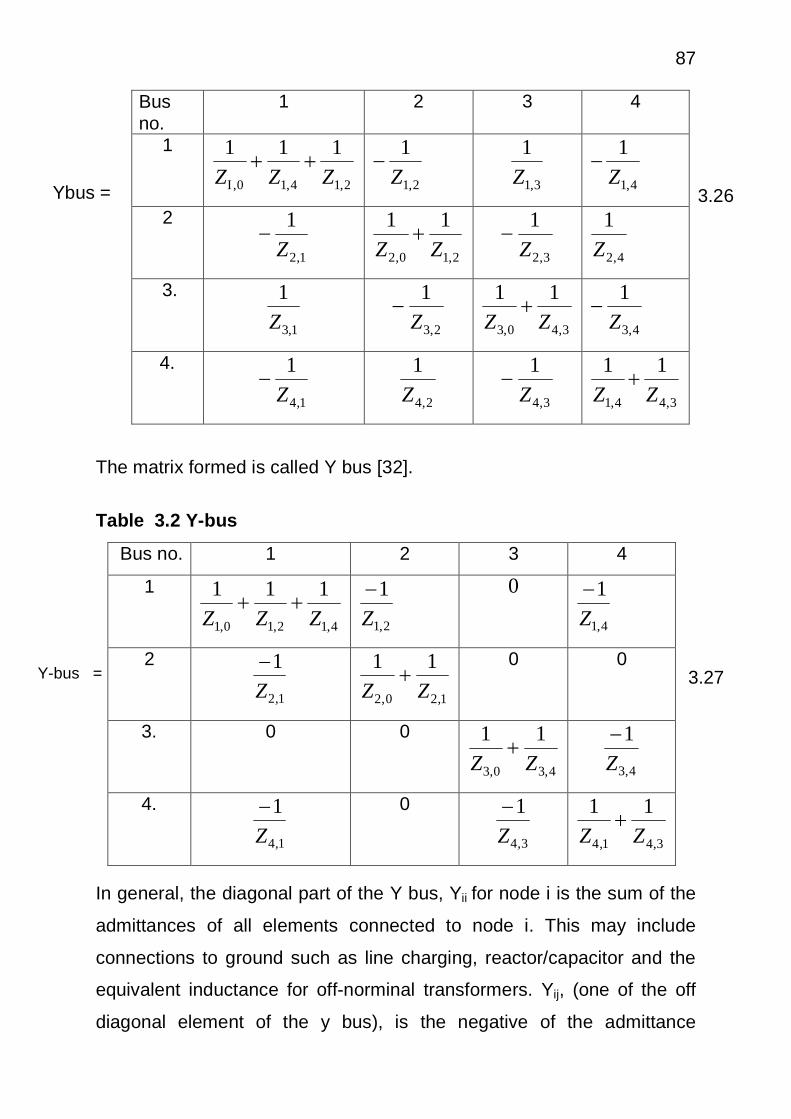
87
Bus no.
1 2 3 4
1
2,14,10,
111ZZZ
2,1
1Z
3,1
1Z
4,1
1Z
2
1,2
1Z
2,10,2
11ZZ
3,2
1Z
4,2
1Z
3.
1,3
1Z
2,3
1Z
3,40,3
11ZZ
4,3
1Z
4.
1,4
1Z
2,4
1Z
3,4
1Z
3,44,1
11ZZ
The matrix formed is called Y bus [32].
Table 3.2 Y-bus
Bus no. 1 2 3 4
1
4,12,10,1
111ZZZ
2,1
1Z
0
4,1
1Z
2
1,2
1Z
1,20,2
11ZZ
0 0
3. 0 0
4,30,3
11ZZ
4,3
1Z
4.
1,4
1Z
0
3,4
1Z
3,41,4
11ZZ
In general, the diagonal part of the Y bus, Yii for node i is the sum of the
admittances of all elements connected to node i. This may include
connections to ground such as line charging, reactor/capacitor and the
equivalent inductance for off-norminal transformers. Yij, (one of the off
diagonal element of the y bus), is the negative of the admittance
Y-bus =
Ybus = 3.26
3.27

88 between node i and node j. The zeros in figure 3.27 shows that there is
no link between the buses.
Gauss-Siedel load flow (GSLF)
The equations can be visualized using a sample of 4-bus distribution
system.
In a distribution system the total shunt admittance of the line is
divided into two equal parts placed at the sending and receiving ends of
the line. It is important therefore to examine the issue using the
equivalent representation shown in figure 3.4 [40].
Fig. 3.4 Nominal - circuit.
To obtain an expression for sending voltage, we note that the current in
the capacitance at the receiving end is 2YVR and the current in the series
arm is. 2YVI R
R Thus:
RRR
S VZIYVV
2 3.28
RRR VZIYZV
2
3.29
RRR ZIVYZV
2
3.30
RR ZIVIZY
2 3.31
VS
IS
2Y 2
Y VR
IR Z
-
+

89
RRS
S IYVYVI 22
3.32
Substituting equation 3.31 into equation 3.32 we get:
RR
RRS IYVYZIVIZYI
222 3.33
RRRRR IYVZYIYVYZYV
2224
3.34
RRRR IZYIYVVZY
222
4
2
3.35
IZYIIZYYV RR 24
3.36
Where: IS is sending current to the bus
Vs is sending voltage to the bus
VR is receiving voltage to the bus
IR is receiving current to the bus
The admittance to the bus S
S
VIY 3.37
The distribution system is characterized by a system of n nonlinear
equations of the form in equation 3.37. Therefore equation 3.37 can be
written as
[Ibus] = [Ybus] [Vbus] 3.38
Where: n is the number of buses in the system.
Ibus is the bus current vector
Vbus is the bus voltage vector
Ybus is the bus admittance

90 Y bus for power system is in complex number.
jxrjxr
jxrjxrYij
*11 3.39
Where r is the real part and x is the imaginary part.
From Equation 3.38 it is clear that the current at the ith bus is given by
jijn
jj
n
ji VYYiiViYijVjI
111
3.40
thus jij
n
jj
i VYIViYii
11
3.41
Solving for Vi gives: )(1
11
jijn
jj
iii
i VYIY
V
3.42
and recalling Equation 2.30 where, Ii = i
ii
VjQP
3.43
Substituting equation 3.43 into equation 3.42 we get
)(1
11
jijn
jji
ii
iii VY
VjQP
YV
3.44
On substituting equation 3.43 into equation 3.40 and i=1
4143132121111
*1 VYVYVYVYV
jQP
3.45
Solving for V1 gives
)]([1414313212*
1
11
111 VYVYVY
VjQP
YV
3.46
Also 424323222121*2
22 VYVYVYVYV
jQP
3.47

91 Solving for V2 gives.
)]([1424323121
2*
22
222 VYVYVY
VjQP
YV
3.48
Also 434333232131*3
33 VYVYVYVYV
jQP
3.49
Solving for V3 gives,
)]([1424222121*
3
33
333 VYVYVY
VjQP
YV
3.50
Equation 3.44 involves only the bus voltages and apparent powers as
variables, and can be solved iteratively using the most recent estimates
of the bus voltage until the change in bus voltage is smaller than some
specified tolerance, ε. The iterative process employed to solve this
system of equations is known as Gauss – Seidel method, and forms the
basis of the load flow analysis used in this project. It should be pointed
out that the equation 3.44 in only used for load buses (buses where the
real and reactive power are specified). However, since distribution
systems rarely contain generators this is sufficient. In order to reduce the
computing time, several calculations can be performed before iterative
produce is initiated. These calculations only involve the constant
quantities of the admittance matrix values and bus loads, and are given
as follows ii
ijI
ii
iii Y
YB
YjQPA
,)(
3.51
Substitution of these equations in to equation 3.44 gives.
)(11
jijn
ji
ii
iji VY
VjQP
YV
jijn
jjji
ii VB
VAV
1
3.52

92 A load flow algorithm based on equation 3.51 and 3.52 and having a
convergence tolerance, ε = 10-6 shall be implemented using MATLAB.
It should be remembered that the Gauss-Seidel method is an iterative
technique, and may require a large number of iterations to converge (or
may even fail to converge) on a solution.
In this project, the load flow with the aid of MATLAB is used to
determine the voltage at each bus, current at each bus, I2R loss and I2X
(Reactive) power loss at each bus in Kilowatts.
3.4 LOAD VARIATION WITH TIME
It is well known that the loads on a power system are dynamic, that
is, they vary over time. These variations may occur quite rapidly (during
switching on or off parts of the power system), or may take place more
gradually, as in the case of daily load variations. It is these gradual
changes due to load variations that are of interest in this project. System
loads may be broadly grouped into three load categories: residential,
commercial and industrial. As well, the total load at a particular point in
the distribution system may be some combination of these load types. It
has been suggested [11] that the year can be divided into 12 periods to
accommodate the load variations due to the seasons (Raining and Dry
seasons), the week (weekday and weekend), and the daily load level
(peak load period, and off peak-load period).
Loads tend to follow the same patterns for each of these three
season periods. Daily load profiles within each season will differ
according to whether it is a weekday or a weekend /holiday. Daily load
profiles will also vary depending on the type of the load: Residential,
commercial or industrial. Daily load also will differ according to time of
the day, peak period (07:31am to 10:30pm) and off-peak period
(10:31pm to 07:30am the next day). The system loads are considered to
be constant during each time interval [25], [41].

93 Daily load profiles during each season can be further divided into four
periods: weekday peak period, weekday off-peak period, weekend peak
period, and weekend off- peak period. Hence, the annual load variation
of each of the three load type can be divided into twelve periods, and the
load variation of the total load can be determined by the weighted sum of
the three load types during each period, where the weights are
determined from the proportion of each load type at the load point.
In this project, the twelve period model was recommended. Using
the load conversion factors presented by Abdel [20], the load profile for
each of the twelve periods was obtained. For the system studied in this
project, the load at each bus was assumed to consist of 15% industrial,
25% commercial load, and 60% residential load. To more realistically
model the unpredictability of the loads, the load at each bus can be
multiplied by a uniformly distributed random number between 0.85 and
1.15. This technique also eliminates reliance on the unrealistic
approximations used by many researchers that:
(i) The loads at every bus vary in the same proportion and
(ii) The reactive power consumed by the load is a fixed fraction of
the real power consumed by the load.
3.5 DERIVATION OF POWER LOSS REDUCTION EQUATIONS
Consider the supply to the inductive load of Figure 3.5 below. The
phasor diagram (a) Shows the current 11 lagging by an angle ø1. The
active and reactive components are 11 Cos θ1 and 11 sin θ1 respectively.
The addition of the capacitor (Diagram (b)) causes an additional current
IC to be drawn from the supply, but as the current is almost entirely
reactive and leading the voltage by 90o it will reduced the reactive
component 11sinθ1 of the load to a smaller value 12sinθ2. This means
that the current 12 taken from the supply has also been reduced and the
new phase angle is ø2, which gives an improved power factor, Cos θ2.

94 It will be seen that the true power taken from the supply has not altered
and 11 Cos θ1 = 12 Cos θ2. Also, 12 is the resultant of the phasor sum of
11 and 1c.
It can be seen also that the current 12 flows from X to Y, that is, to
the point at which the capacitor is connected, but beyond the capacitor,
from Y to Z, the current and power factor are still the original values of 11
and Cos θ1. Thus, the power factor is improved only on the supply side
of the capacitor [14], [42].
From figure 3.5
(b) it is seen that:
11
111 cos1
1tan Sin
3.53
11111 tancos1sin1 3.54
11
222 cos1
sin1tan also 3.55
I2sin 2 = (I1cos1)tan 2 3.56
also I2cos2 = (I1cos1) (in-phase component of voltage 3.57
Capacitor current Ic = I1sin1 – I2sin2 3.58
Since addition of capacitor causes additional current 1c to be draw
from the supply, Reactive Kilovolt amperes (KVAR) = V1c Sin θ
When the current leads the voltage by 900 ie θ = 90o, then
Kvar = V1c 3.59
VKVarIc 3.60

95 Where V is the line voltage.
For a 3 – phase work, Ic = V
k3
var 3.61
Fig. 3.5 Effect of capacitor in parallel with an inductive load: (a) an inductive load, (b) adding a capacitor 3.5.1 I2R LOSS REDUCTION DUE TO CAPACITOR
The active power loss due to a current I1 flowing through a circuit with
resistance R is I12R, and the energy loss during the time t is 112Rt.
Assuming a power factor cos , the 12R loss may be divided into two
components:
(i) 112R loss due to active component of current
(ii) 112R loss due to reactive component of current.
Thus power loss before addition of capacitor is
62.3sin1cos11 211
211
21 RRR
V fHZ
Inductive Load. V
fHZ
Inductive Load. Capacitor
Ic
X I2 Y I1 Z
I1
V
I1 sin 1 (a)
11cos 1
I1
V
I2 sin 2 (b)
1
11cos 1 =12cos 2
I2
I1 sin 1
Ic 2
I1
1 Ic

96 When a capacitor with current IC is applied, resulting in a new line
current 12, then power loss after addition of capacitor is
c
RRR1sin1sin13.44,equation from
.sin1cos11
1122
222
222
22
RRR 2211
222
22 1sin1cos11 3.65
RRRR Cc2
112
112
22 11sin12sin1cos1 3.66
But 2211 cos1cos1
Power loss reduction RRL 22
21 11
RRRR 211
222
211
211 sin1cos1sin1cos1
RR CC2
11 11sin12 3.67
RRL CC2
11 11sin12 3.68
RCC2
11 11sin21 3.69
RCC 11sin21 11 3.70
Considering the loss reduction based on the combination of active
and reactive components of current, the total power loss PL in the
distribution system is given by:
riIriIIP riaiM
iiri
M
iL
22
1
2
1
3.71
where M is the total number of the system section, Ii is the current
flowing in the ith section having active and reactive components of Iai
and Iri respectively and ri is the ith section resistance.
As the losses due to the active component of the flowing current
cannot be affected by the compensating capacitors (Zero power factor
element), the only term that is of interest are the losses due to the
reactive component of the system current, iri r2 [20]
3.63
3.64

97
The losses due to the reactive currents PrL can be written as;
m
irL riIriP
1
2 3.72
3.6 DERIVATION OF ECONOMICAL POWER FACTOR.
Economical power factor is the power factor at which the gain or
savings obtained from installing capacitor banks for power loss reduction
in a distribution system is equal to or greater than the cost of the
capacitor banks and their cost of installation in the system [1]. It is also
the power factor at which the net savings is maximum.
Fig 3.6 Power triangle for Economical power factor and net savings
Suppose a consumer is charged at NA per KVA maximum
demand plus a flat rate per KWh. Further suppose he is taking power of
P, kw at a power factor of cos .
1 2
Power in kw (P)
KVA2
KVA1
1
E
KVAR2
F
C
KVAR1
o

98 As shown in figure 3.6 his
KVA1=
1COSP
3.73
KVAR1= Ptan 1 3.74
Suppose by installing capacitors he improves his power factor to cos 2
(his power consumption P remaining the same). In that case his
KVA2 =2COS
P 3.75
KVAR2 =P tan 2 3.76
R education in his KVA maximum demand is
= (KVA1 –KVA2) 3.78
=
21 COSP
COSP 3.79
Since charge is NA per KVA maximum demand, his annual saving on his
account is = A
21 COSP
COSP 3.80
His KVAR is reduced from KVAR1 to KVAR2, the difference KVAR1-
KVAR2= P tan 1 -P tan 2 being neutralized by the leading KVAR
supplied by the capacitors. Leading KVAR supplied by the static
capacitors
= P tan 1 -P tan 2 3.81
The cost of power factor improvement equipment is taken into
account by way of interest on capital required to install it plus
depreciation and maintenance expenses. Thus, the greater the KVAR
reduction, the more costly the P.F improvement capacitor and hence
greater the charge on interest on capital outlay and depreciation. A point
is reached in practice when any further improvement in power factor,
cost more than saving in the bill. Hence it is necessary for the consumer

99 to find out the value of power factor at which his net savings will be
maximum. The value can be found if:
(i) Annual charge per KVA maximum demand and
(ii) The cost per KVAR rating of capacitor are known.
If the cost per KVAR of capacitor is NB and the rate of interest and
depreciation is U percent per year, then its cost per annum is
21 tantan100
PPUB
3.82
Assuming CUB
100
3.83
Cost per annum = C 21 tantan PP 3.84
Where B * U is cost per KVAR multiplied by depreciation factor of U%
Net annual saving S is
S= A
21 COSP
COSP -C(Ptan 21 tan P ) 3.85
This net savings is maximum when 2d
ds = 0 3.86
Therefore 22 d
ddds
[A
21 COSP
COSP
-C(P tan 1-P tan 2)] 3.87
=2d
d [AP(Sec 1-Sec 2)-CP(tan 21 tan ]=0 3.88
= -AP(Sec 22
22 tan Seccp = 0 3.89
- AP Sec 0tan 22
22 CPSec 3.90
AP Sec 22
22 tan CPSec 3.91
A Sec 22
22 tan CSec 3.92
= 22tan CSecA 3.93
=AC
2
2
sectan
3.94
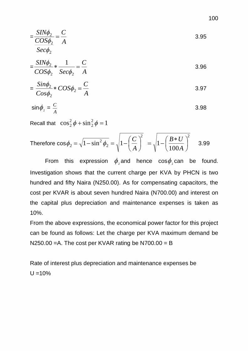
100
=AC
SecCOSSIN
2
2
2
3.95
=AC
SecCOSSIN
22
2 1
3.96
= ACCOS
CosSin
22
2
3.97
sin 2 = AC 3.98
Recall that 1sincos 22
22
Therefore cos22
22
2 10011sin1
AUB
AC 3.99
From this expression 2 and hence cos 2 can be found.
Investigation shows that the current charge per KVA by PHCN is two
hundred and fifty Naira (N250.00). As for compensating capacitors, the
cost per KVAR is about seven hundred Naira (N700.00) and interest on
the capital plus depreciation and maintenance expenses is taken as
10%.
From the above expressions, the economical power factor for this project
can be found as follows: Let the charge per KVA maximum demand be
N250.00 =A. The cost per KVAR rating be N700.00 = B
Rate of interest plus depreciation and maintenance expenses be
U =10%
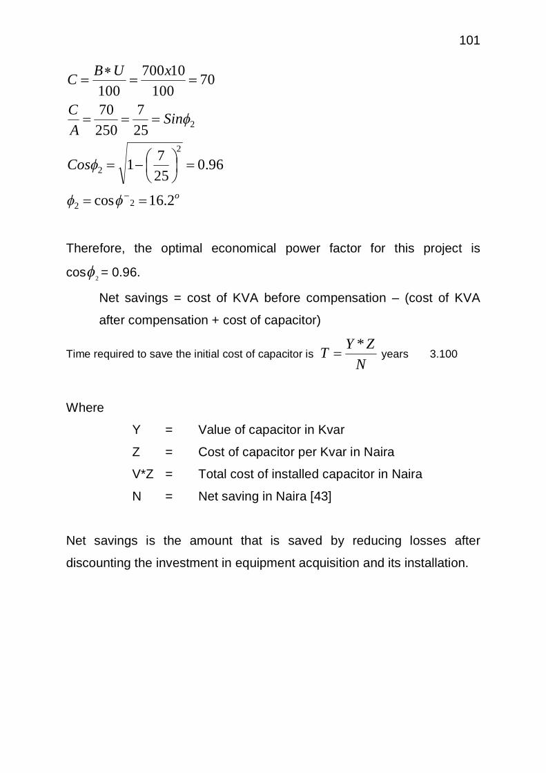
101
o
Cos
SinAC
xUBC
2.16cos
96.02571
257
25070
70100
10700100
22
2
2
2
Therefore, the optimal economical power factor for this project is
cos 2 = 0.96.
Net savings = cost of KVA before compensation – (cost of KVA
after compensation + cost of capacitor)
Time required to save the initial cost of capacitor is N
ZYT * years 3.100
Where
Y = Value of capacitor in Kvar
Z = Cost of capacitor per Kvar in Naira
V*Z = Total cost of installed capacitor in Naira
N = Net saving in Naira [43]
Net savings is the amount that is saved by reducing losses after
discounting the investment in equipment acquisition and its installation.

102
CHAPTER FOUR
4.0 APPLICATION OF THE PROPOSED METHOD
The described method is applied to a 34 bus three phase radial
feeder with lateral branches shown in fig. 4.1. The feeder considered in
the distribution system is the 11KV feeder in the Thinker’s Corner
injection substation which caries an average load of 4636.5kw and
2873.5kvar distributed over 34 main load points along the distribution
feeder line: 60% residential, 25% commercial and 15% industrial loads.
The main feeder is connected to many sub-feeders which in turn carry
radial loads.
Figure 4.1 shows the one-line diagram of 11KV Thinker’s Corner
injection substation distribution feeder under study with its lateral
branches.
The substation line voltage is 11KV. The node numbers and the
appropriate active and reactive power loads are given in Table 4.1
(Distribution data)
The software implementation procedure has been done using
MATLAB environment for the ease of operating with complex numbers;
the load flow results from our software are shown in tabular form in the
subsequent pages 91 to 108.
All the calculations have been carried out in per unit system with
the three phase base SB = 100MVA, VB = 11KV.
The total installed power is 6.0MVA with an average power factor of
0.85.

103
Fig 4.1 One – Line Diagram of 34 Bus Thinkers’ Corner Distribution System with Lateral Branches.
Orthopoedics
Hospital and Ecumenical
Schools.
1
27 26 25 24 23 22 34
33
32
31
30
29
2813
14
15
16
2120
19
1817
2 3 4 5 6 7 8 9 10 11 12
6.0MVA, 33/11(KV)
750Kvar capacitor
GRA
Abakpa
450Kvar Capacitor
Army B
arrac
ks
Nike

104 Table 4.1 Thinker’s Corner 11kV Feeder Distribution System Data
Table 4.1.1 Bus Data Bus No Load
P Kw Q(Kvar) 1 0 0 2 230 142.5 3. 0 0 4 230 142.5 5 230 142.5 6 0 0 7 0 0 8 230 1425 9 230 142.5 10 0 0 11 230 142.5 12 137 84 13 72 45 14 72 45 15 72 45 16 13.5 7.5 17 230 142.5 18 230 142.5 19 230 142.5 20. 230 142.5 21 230 142.5 22 230 142.5 23 230 142.5 24 230 142.5 25 230 142.5 26 230 142.5 27 137 85 28 75 48 29. 75 48 30 75 48 31 57 34.5 32 57 34.5 33 57 34.5 34 57 34.5
Source: Thinker’s Corner Injection Substation of PHCN Enugu.

105 Table 4.1.2 Line Data
Line Impedance
Length
(Km)
Impedance
Line No Kmr
KmX
r +jX
1-2 0.195 0.080 0.60 0.117 + j0.048 2-3 0.195 0.080 0.55 0.10725 + j0.044 3-4 0.299 0.083 0.55 0.16445+ j0.04565 4-5 0.299 0.083 0.50 0.1495 + j0.0415 5-6 0.299 0.083 0.50 0.1495 + j0.0415 6-7 0.524 0.090 0.60 0.3144+j0.054 7-8 0.524 0.090 0.40 0.2096+j0.036 8-9 0.524 0.090 0.60 0.3144+j0.054 9-10 0.524 0.090 0.40 0.2096+j0.036 10-11 0.524 0.090 0.25 0.131+ j0.0225 11-12 0.524 0.090 0.20 0.1048 + j0.018 3-13 0.524 0.090 0.30 0.1572+j0.027 13-14 0.524 0.090 0.40 0.2096 + j0.036 14-15 0.524 0.090 0.20 0.1048 + j0.018 15-16 0.524 0.090 0.10 0.0524 + j0.009 6-17 0.299 0.083 0.60 0.1794 + j0.0498 17-18 0.299 0.083 0.55 0.16445 + j0.04565 18-19 0.378 0.086 0.55 0.2079 + j0.0473 19-20 0.378 0.086 0.50 0.189 + j0.043 20-21 0.378 0.086 0.50 0.189+j0.043 21-22 0.524 0.090 0.50 0.262 + j0.045 22-23 0.524 0.090 0.50 0.262 + j0.045 23-24 0.524 0.090 0.60 0.3144 + j0.054 24-25 0.524 0.090 0.40 0.2096+ j0.036 25-26 0.524 0.090 0.25 0.131+j0.0225 26-27 0.524 0.090 0.20 0.1048 + j0.018 27-28 0.524 0.090 0.30 0.1572 + j0.027 28-29 0.524 0.090 0.30 0.1572 + j0.027 29-30 0.524 0.090 0.30 0.1572 + j0.027 10-31 0.524 0.090 0.30 0.1572 + j0.027 31-32 0.524 0.090 0.40 0.2096 + j0.036 32-33 0.524 0.090 0.30 0.1572 + j0.027 33-34 0.524 0.090 0.20 0.1048 + j0.018
Source: Thinker’s Corner Injection Substation of PHCN Enugu.

106 4.1 LOAD FLOW RESULTS Table 4.1.3 Voltages and Currents in the Distribution System Bus Voltages (per Unit) Line Currents (Per Unit) Line Currents (A) Load Currents (Per Unit) Load Currents (A) V1 = 1.00 V2 = 0.9941 + 0.0009i V3 = 0.9890 + 0.0017i V4 = 0.9820 + 0.0037i V5 = 0.9761 + 0.0053i V6 = 0.9704 + 0.0069i V7 = 0.9666 + 0.0084i V8 = 0.9644 + 0.0092i V9 = 0.9620 + 0.0102i V10 = 0.9608 + 0.0107i V11 = 0.9603 + 0.0108i V12 = 0.9602 + 0.0109i V13 = 0.9887 + 0.0018i V14 = 0.9884 + 0.0020i V15 = 0.9883 + 0.0020i V16 = 0.9883 + 0.0020i V17 = 0.9659 + 0.0081i V18 = 0.9622 + 0.0092i V19 = 0.9581 + 0.0105i V20 = 0.9548 + 0.0116i V21 = 0.9519 + 0.0125i V22 = 0.9486 + 0.0138i V23 = 0.9459 + 0.0148i V24 = 0.9434 + 0.0158i V25 = 0.9422 + 0.0163i V26 = 0.9417 + 0.0165i V27 = 0.9416 + 0.0165i V28 = 0.9664 + 0.0085i V29 = 0.9662 + 0.0085i V30 = 0.9661 + 0.0086i V31 = 0.9604 + 0.0108i V32 = 0.9601 + 0.01090i V33 = 0.9599 + 0.0110i V34 = 0.9599 + 0.0110i
i2 = 0.0486 – 0.0294i i3 = 0.0463 – 0.0280i i4 = 0.0439 – 0.0265i i5 = 0.0416 – 0.0251i i6 = 0.0392 – 0.02361i i7 = 0.0134 – 0.0081i i8 = 0.0110 – 0.0066i i9 = 0.0086 – 0.0052i i10 = 0.0062 – 0.0037i i11 = 0.0038 – 0.0023i i12 = 0.0014 – 0.0009i i13 = 0.0023 – 0.0014i i14 = 0.0016 – 0.0010i i15 = 8.6615e-004-5.2947e-004i i16 = 1.3704e-004 -7.5561e-005i i17 = 0.0258 – 0.0155i i18 = 0.0234 – 0.0141i i19 = 0.0210 – 0.0126i i20 = 0.0186 – 0.0111i i21 = 0.0162 – 0.0097i i22 = 0.0138 – 0.0082i i23 = 0.0113 – 0.0068i i24 = 0.0089 – 0.0053i i25 = 0.0064 – 0.0038i i26 = 0.0040 – 0.0023i i27 = 0.0014 – 0.0009i i28 = 0.0023 – 0.0015i i29 = 0.0016 – 0.0010i i30 = 7.8099e-004 – 4.8990e-004i i31 = 0.0024 -0.0014i i32 = 0.0018 – 0.0011i i33 = 0.0012 – 0.0007i i34 = -5.9844e-004 – 3.5254e-004i
Ib = 5248.6 I2 = 2.5498e+002 - 1.5424e+002i I3 = 2.4283e+002 - 1.4673e+-002i i4 = 2.3063e+002 – 1.3918e+002i i5 = 2.1831e+002 – 1.2402e+002i i6 = 2.0590e+002 – 1.2402e+002i i7 = 70.2534 – 42.5449i i8 = 57.9617 – 34.8303i i9 = 45.3718 – 27.1957i i10 = 32.7424 – 19.5543i i11 = 20.1972 – 12.1519i i12 = 7.5412 – 4.5060i i13 = 12.2007 – 7.5430i i14 = 8.3741 – 5.1612i i15 = 4.5463 – 2.7790i i16 = 0.7184 – 0.3966i i17 = 1.3565e+002-8.1474e+001i i18 = 1.2308e+002 – 7.3836e+001i i19 = 1.1046e+002 – 6.6183e+001i i20 = 97.7813 – 58.5160i i21 = 85.0451 – 50.8370i i22 = 72.2624 – 43.1480i i23 = 59.4251 – 35.4503i i24 = 46.5425 – 27.7454i i25 = 33.6175 – 20.0337i i26 = 20.6723 – 12.3188i i27 = 7.7190 – 4.6026i i28 = 12.2934 – 7.7141i i29 = 8.1970 – 5.1428i i30 = 4.0993 – 2.5713i i31 = 12.5477 – 7.4019i i32 = 9.4122 – 5.5516i i33 = 6.2759 – 3.7011i i34 = 3.1393 – 1.8502i
il2 = - 0.0023 + 0.0014i il3 = - 0.0000 + 0.0000i il4 = - 0.0023 + 0.0014i il5 = - 0.0024 + 0.0014i il6 = - 0.0000 + 0.0000i il7 = - 0.0000 + 0.0000i il8 = - 0.0024 + 0.0014i il9 = - 0.0024 + 0.0014i il10 = - 0.0000 + 0.0000i il11 = - 0.0024 + 0.0014i il12 = - 0.0014 - 0.0009i il13 = - 7.2909e - 004 +4.5379e-004i i114 = - 7.2909e - 004 + 4.5379e-004i il15 = - 7.2909e-004+4.5379e-004i il16 = - 1.3675e-004+7.56lle-005i il17 = - 0.0024 + 0.0014i il18 = - 0.0024 + 0.0014i il19 = - 0.0024 + 0.0014i il20 = - 0.0024 + 0.0014i il21 = - 0.0024 + 0.0014i il22 = - 0.0024 + 0.0014i il23 = - 0.0024 + 0.0014i il24 = - 0.0024 + 0.0014i il25 = - 0.0024 + 0.0014i il26 = - .00024 + 0.0014i il27 = - 0.0014 – 0.0009i il28 = - 7.8056e – 004 + 4.8988e-004i il29 = - 7.8056e – 004 + 4.8988e-004i il30 = - 7.8056e – 004 + 4.8988e-004i il31 = - 5.9744e-004 + 3.5251e-004i il32 = - 5.9744e-004 + 3.5251e-004i il33 = - 5.9744e-004 + 3.5251e-004i il34 = - 5.9744e-004 + 3.5251e-004i
il2 = - 12.1500 + 7.5122i il3 = - 0.0000 + 0.0000i il4 = - 12.3207 + 7.5702i il5 = - 12.4096 + 7.5951i il6 = - 0.0000 + 0.0000i il7 = - 0.0000 + 0.0000i il8 = - 12.4096. + 7.5951i il9 = - 12.4096 + 7.5122i il10 = - 0.0000 + 0.0000i il11 = - 12.4096 + 7.5122i il12 = - 7.5400 – 4.5063i il13 = - 3.8267 + 2.3818i il14 = - 3.8267 + 2.3818i il15 = - 3.8267 + 2.3818i il16 = - 0.7178 + 0.3969i il17 = - 12.4096 + 7.5951i il18 = - 12.4096 + 7.5951i il19 = - 12.4096 + 7.5951i il20 = - 12.4096 + 7.5951i i121 = - 12.4096 + 7.5951i i122 = - 12.4096 + 7.5951i i123 = - 12.4096 + 7.5951i i124 = - 12.4096 + 7.5951i i125 = - 12.4096 + 7.5951i i126 = - 12.4096 + 7.5951i i127 = - 7.5400 – 4.5063i i128 = - 4.0969 + 2.5712i i129 = - 4.0969 + 2.5712i i130 = - 4.0969 + 2.5712i i131 = - 3.1358 + 1.8502i i132 = - 3.1358 + 1.8502i i133 = - 3.1358 + 1.8502i i134 = - 3.1358 + 1.8502i
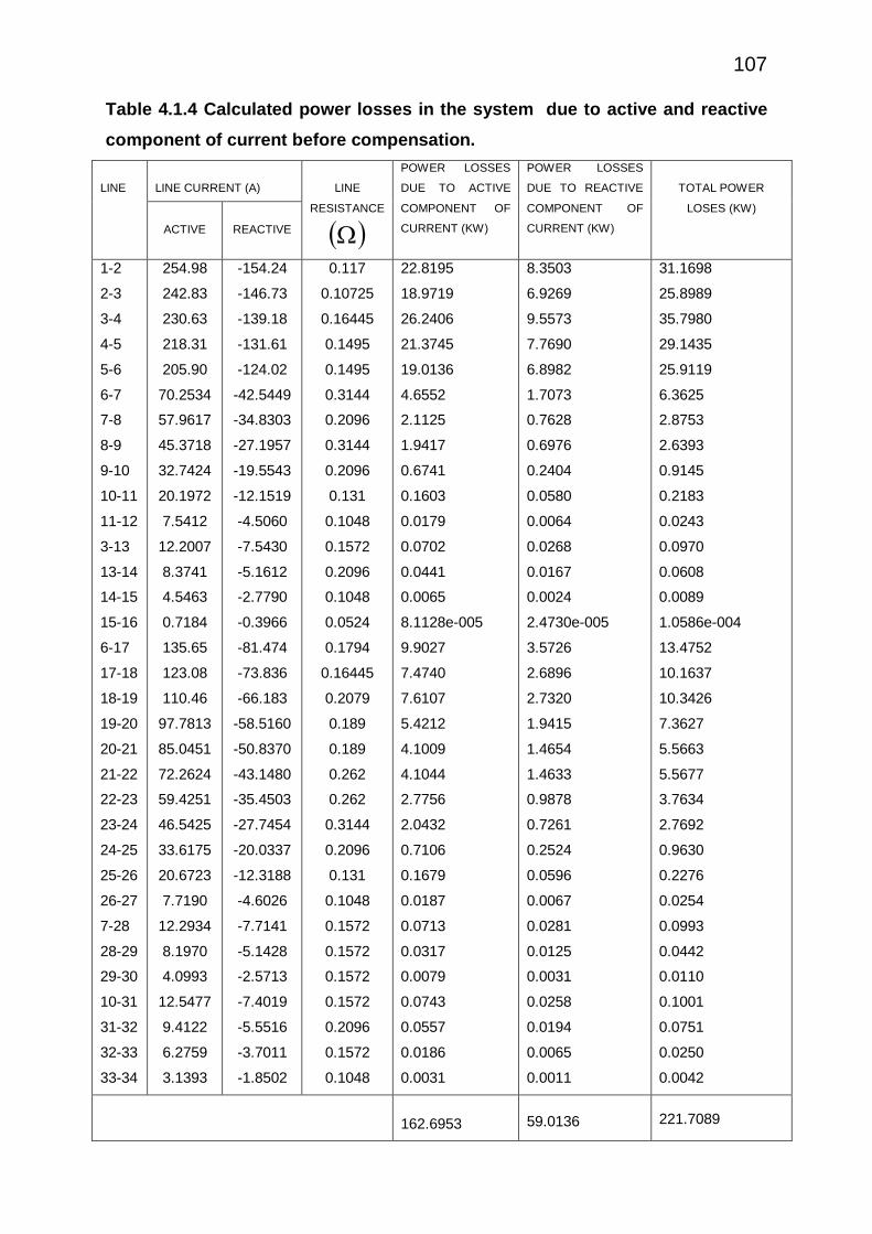
107 Table 4.1.4 Calculated power losses in the system due to active and reactive
component of current before compensation.
LINE
LINE CURRENT (A)
LINE
RESISTANCE
POWER LOSSES
DUE TO ACTIVE
COMPONENT OF
CURRENT (KW)
POWER LOSSES
DUE TO REACTIVE
COMPONENT OF
CURRENT (KW)
TOTAL POWER
LOSES (KW)
ACTIVE
REACTIVE
1-2
2-3
3-4
4-5
5-6
6-7
7-8
8-9
9-10
10-11
11-12
3-13
13-14
14-15
15-16
6-17
17-18
18-19
19-20
20-21
21-22
22-23
23-24
24-25
25-26
26-27
7-28
28-29
29-30
10-31
31-32
32-33
33-34
254.98
242.83
230.63
218.31
205.90
70.2534
57.9617
45.3718
32.7424
20.1972
7.5412
12.2007
8.3741
4.5463
0.7184
135.65
123.08
110.46
97.7813
85.0451
72.2624
59.4251
46.5425
33.6175
20.6723
7.7190
12.2934
8.1970
4.0993
12.5477
9.4122
6.2759
3.1393
-154.24
-146.73
-139.18
-131.61
-124.02
-42.5449
-34.8303
-27.1957
-19.5543
-12.1519
-4.5060
-7.5430
-5.1612
-2.7790
-0.3966
-81.474
-73.836
-66.183
-58.5160
-50.8370
-43.1480
-35.4503
-27.7454
-20.0337
-12.3188
-4.6026
-7.7141
-5.1428
-2.5713
-7.4019
-5.5516
-3.7011
-1.8502
0.117
0.10725
0.16445
0.1495
0.1495
0.3144
0.2096
0.3144
0.2096
0.131
0.1048
0.1572
0.2096
0.1048
0.0524
0.1794
0.16445
0.2079
0.189
0.189
0.262
0.262
0.3144
0.2096
0.131
0.1048
0.1572
0.1572
0.1572
0.1572
0.2096
0.1572
0.1048
22.8195
18.9719
26.2406
21.3745
19.0136
4.6552
2.1125
1.9417
0.6741
0.1603
0.0179
0.0702
0.0441
0.0065
8.1128e-005
9.9027
7.4740
7.6107
5.4212
4.1009
4.1044
2.7756
2.0432
0.7106
0.1679
0.0187
0.0713
0.0317
0.0079
0.0743
0.0557
0.0186
0.0031
8.3503
6.9269
9.5573
7.7690
6.8982
1.7073
0.7628
0.6976
0.2404
0.0580
0.0064
0.0268
0.0167
0.0024
2.4730e-005
3.5726
2.6896
2.7320
1.9415
1.4654
1.4633
0.9878
0.7261
0.2524
0.0596
0.0067
0.0281
0.0125
0.0031
0.0258
0.0194
0.0065
0.0011
31.1698
25.8989
35.7980
29.1435
25.9119
6.3625
2.8753
2.6393
0.9145
0.2183
0.0243
0.0970
0.0608
0.0089
1.0586e-004
13.4752
10.1637
10.3426
7.3627
5.5663
5.5677
3.7634
2.7692
0.9630
0.2276
0.0254
0.0993
0.0442
0.0110
0.1001
0.0751
0.0250
0.0042
162.6953
59.0136
221.7089

108 Table 4.1.5 Power losses due to reactive component of load
current before compensation (pf.= 0.85).
LINE
LOAD CURRENT (A) RESISTANCE
( )
POWER LOSSES DUE TO
REACTIVE COMPONENT OF
LOAD CURRENTS (KW) (Ir2LR) Active Reactive 1-2
2-3
3-4
4-5
5-6
6-7
7-8
8-9
9-10
10-11
11-12
12-13
13-14
14-15
15-16
16-17
17-18
18-19
19-20
20-21
21-22
22-23
23-24
24-25
25-26
26-27
27-28
28-29
29-30
30-31
31-23
32-33
33-34
il2 = - 12.1500
il3 = 0
il4 = - 12.3207
il5 = - 12.4096
il6 = 0
il7 = 0
il8 = - 12.4096
il9 = - 12.4096
il10 = 0
il11 = - 12.4096
il12 = - 7.5400
il13 = - 3.8267
il14 = - 3.8267
il15 = - 3.8267
il16 = - 0.7178
il17 = - 12.4096
il18 = - 12.4096
il19 = - 12.4096
il20 = - 12.4096
i121 = - 12.4096
i122 = - 12.4096
i123 = - 12.4096
i124 = - 12.4096
i125 = - 12.4096
i126 = - 12.4096
i127 = - 7.5400
i128 = - 4.0969
i129 = - 4.0969
i130 = - 4.0969
i131 = - 3.1358
i132 = - 3.1358
i133 = - 3.1358
i134 = - 3.1358
7.5122i
0
7.5702i
7.5951i
0
0
7.5951i
7.5122i
0
7.5122i
4.5063i
2.3818i
2.3818i
2.3818i
0.3969i
7.5951i
7.5951i
7.5951i
7.5951i
7.5951i
7.5951i
7.5951i
7.5951i
7.5951i
7.5951i
4.5063i
2.5712i
2.5712i
2.5712i
1.8502i
1.8502i
1.8502i
1.8502i
0.117
0.22425
0.3887
0.5382
0.6877
1.0021
1.2117
1.5261
1.7357
1.8667
1.9715
0.38145
0.59105
0.69585
0.74825
0.8671
1.03155
1.23945
1.42845
1.61745
1.87945
2.14145
2.45585
2.66545
2.79645
2.90125
1.1593
1.3165
1.4737
1.8929
2.1025
2.2597
2.3645
6.6028
0
22.2754
31.0464
0
0
69.8978
88.0341
0
107.6819
40.0339
2.1639
3.3529
3.9475
0.1178
50.0193
59.5057
71.4985
82.4011
93.3037
108.4174
123.5310
141.6674
153.7583
161.3152
58.9137
7.6642
8.7034
9.7427
6.4797
7.1972
7.7354
8.0941

109
Table 4.1.6 Power Losses and Loss Reduction due to Addition of Capacitor Banks on Nodes 26, 11, and the overall Power Losses and loss reduction due to capacitor banks on nodes 26 and 11 combined.
Power Losses and Loss reduction due to capacitor banks on node 26 only
Power Losses and Loss Reduction due to Capacitor Banks on node II only
Overall Power losses, and loss reduction due to capacitor banks at node 26 and 11 combined.
Capacitor
Bank on Node
26 (Kvar)
Power
factor
Power
Loss
(KW)
Power Loss
Reduction
(KW)
Capacitor Bank
on Node 11
(Kvar)
Power
Factor
Power
Loss (KW)
Power Loss
reduction
(KW)
Capacitor
Bank (Kvar)
on Nodes
26 & 11
Power
Factor
Power Loss
(KW)
Power Loss
Reduction (KW)
0
150
300
450
600
750
900
1050
1200
1350
1500
0.85
0.87
0.88
0.90
0.91
0.92
0.94
0.95
0.96
0.97
0.98
221.7
206.9
195.5
187.7
183.4
182.6
185.5
191.6
201.4
214.7
231.5
0
14.9
26.2
34
38.3
39.1
36.4
30.1
20.4
7
-9.8
0
150
300
450
600
750
900
1050
1200
1350
1500
0.85
0.89
0.93
0.96
0.98
1.0
1.0
0.99
0.97
0.94
0.91
221.71
211.78
204.11
198.69
195.54
194.64
196.0
199.62
205.50
213.63
224.03
0.0011
9.93
17.60
23.02
26.17
27.07
25.71
22.09
16.21
8.08
2.32
750 + 0
750 + 150
750 + 300
750 + 450
750 + 600
750 + 750
750 + 900
750 + 1050
750 + 1200
750 + 1350
750 + 1500
0.92
0.94
0.95
0.96
0.97
0.98
0.98
0.99
0.99
1.0
1.0
182.6
176.9
173.5
172.3
173.4
176.8
182.4
190.2
200.3
212.7
227.4
39.1
44.8
48.2
49.4
48.3
44.9
39.3
31.5
21.4
9
-5.7

110 Table 4.1.7 Power Factor and Savings due to the addition of capacitor banks on nodes 26, 11 and nodes 26 and 11 combined
Power Factor & Savings calculations for Capacitor banks on node 26 only
Power Factor & Savings calculations for Capacitor banks on node 11 only
Savings due to capacitor banks at nodes 26 & 11 Combined
Net Savings
(N) x 103 Capacitor
banks on
node 26
Power
Factor
Power
Loss Power
loss
reduction
Savings
(N)
Capacitor
banks on
node 11
Power
factor Power
loss Power
Loss
reduction
Savings
(N)
Capacitor
banks on
nodes 26 & 11
Power
factor
Power
Loss
Power Loss
reduction
0
150
300
450
600
750
900
1050
1200
1350
1500
0.85
0.87
0.88
0.90
0.91
0.92
0.94
0.95
0.96
0.97
0.98
221.7
206.9
195.5
187.7
183.4
182.6
185.5
191.6
201.4
214.7
231.5
0
14.9
26.2
34
38.3
39.1
36.4
30.1
20.4
7
-9.8
0.00
8776.400
16,562.00
23,304.00
28,949.00
33,443.00
36,735.00
38,772.00
39,505.00
38,889.00
36,880.00
0
150
300
450
600
750
900
1050
1200
1350
1500
0.85
0.89
0.93
0.96
0.98
1.0
1.0
0.99
0.97
0.94
0.91
221.71
211.78
204.11
198.69
195.54
194.64
196.0
199.62
205.50
213.63
224.03
0.0011
9.93
17.60
23.02
26.17
27.07
25.71
22.09
16.21
8.08
2.32
0
7940.9
13004
14814
13031
7380.5
-2299.0
-16036
-33721
-55120
-79915
750 + 0
750 + 150
750 + 300
750 + 450
750 + 600
750 + 750
750 + 900
750 + 1050
750 + 1200
750 + 1350
750 + 1500
0.92
0.94
0.95
0.96
0.97
0.98
0.98
0.99
0.99
1.0
1.0
182.6
176.9
173.5
172.3
173.4
176.8
182.4
190.2
200.3
212.7
227.4
39.1
44.8
48.2
49.4
48.3
44.9
39.3
31.5
21.4
9
-5.7
33.4
36.7
38.8
39.5
38.9
36.9
33.4
28.5
22.1
14.2
4.8

111 4.2 RESULTS ANALYSIS. Table 4.1 Shows the Thinker’s Corner 11kv Feeder Distribution System data
Table 4.1.1 Shows the Bus Data
Table 4.1.2 Shows the Line Data
Table 4.1.3 Shows the Voltages and Currents in the Distribution System
Table 4.1.4 Shows the losses due to active and reactive components of
current and both of them yielded a total initial peak power losses of
221.7089kw (162.6953 + 59.0136)kw.
Table 4.1.5 Shows Losses due to reactive components of load current
before compensation. In this table 4.1.5, the sensitive nodes were
identified. The sensitive nodes that have the largest loss due to reactive
component of load current among the five sections of the system are
node 26 and 11 respectively. These are the nodes that capacitors are to
be placed (installed). Since capacitors operate only in reactance, the
loss (59.0136)kw due to reactive component of current in table 4.1.4 is
the loss to be reduced by allocating or placing sizeable capacitors on
nodes 26 and 11.
Table 4.1.6 Shows power losses and loss Reduction due to addition of
capacitor Banks on Nodes 26, 11 and the overall power Losses and
Loss reduction due to capacitor banks on nodes 26 and 11combined.
From the table 4.1.6, the available standard capacitor bank sizes are
(150, 250, 300, 400,450,500, 600,750) Kvar etc.
If we have compensating capacitor size of 750Kvar placed on node 26
only, the optimum power factor of 0.92 is obtained and the minimum
power loss is (182.6kw) with maximum power loss reduction of (39.1kw).
With capacitor size of 750Kvar placed on node 11 only, the optimum
power factor of 1.0 is obtained and the minimum power loss is 194.64kw.
Also the loss reduction is maximum at 27.07kw but with capacitor sizes
of 750Kvar and 450Kvar placed on both nodes 26 and 11respectively

112 and combined, the optimum power factor of 0.96 is attained, the power
loss drops to a maximum of 172.3kw and we also have the maximum
power loss reduction as 49.4kw.
Finally, table 4.1.7 shows the power factor and savings due to the
addition of capacitor banks on nodes 26, 11 and nodes 26 and 11
combined.
When capacitor size of 750Kvar is placed on node 26 only, it attracts
power factor of 0.92, power loss of 182.6kw, power loss reduction of
39.1kw and a savings of thirty three thousand, four hundred and forty
three Naira (N33,443.00) only. When capacitor size of 750Kvar is placed
on node 11 only, it attracts a power factor of 1.0, power loss 194.64kw,
power loss reduction of 27.07Kw and a savings of Seven thousand three
hundred and eighty Naira, five Kobo (N7,380.5) only. The combined
effects of 750Kvar capacitor bank placed at node 26 and 450Kvar
capacitor bank placed at node 11 with regard to net savings in naira (N)
per annum, attracts an optimum power factor of 0.96, power loss of
172.3kw, power loss reduction of 49.4kw and a net savings of thirty nine
thousand five hundred naira (N39,500.00) only per annum.
Considering the loss reduction based on the combination of
active and reactive components of current, the power loss becomes.
kw
rrrIaii
rIIL
p iiii
M
ii
m
Li
6.221
1 222
= the initial peek power loss in the system.

113
Where: M, is the total number of the system sections Ii is the current
flowing in the ith section having active and reactive components of Iai
and Iri respectively and ri is the ith section resistance.
M
iii rIa
1
2 is the loss due to active component of current.
M
iii rIr
1
2 is the loss due to reactive component of current.
It has been shown that node 26 has the highest reactive load
current and then the highest effect on the system losses. Hence it is
called a sensitive node. Now a compensating capacitor C of current Ic is
connected at node 26.
To determine the optimum compensation at node 26, varying size
of capacitor banks are connected and the annual net saving, peak power
loss and peak power loss reduction in the system are calculated. Since
the capacitor size Qc in kvar is known, the power factor is computed
from the expression.
Qc = P(tan 21 tan
yLetx
XP
QP
Qc
C
2
12
12
costan
tantan
2tantan
Where: Qc = Power of capacitor in kvar
P = Active power of the load in kw. For node 26, P= 10 X 230 =
2300kw. For node 11, P= 6 x 230 = 1380kw
TanØ1 = 0.6198,Q1 = 31.79o
TanØ2 = 0.2917, Ø = 16.26o
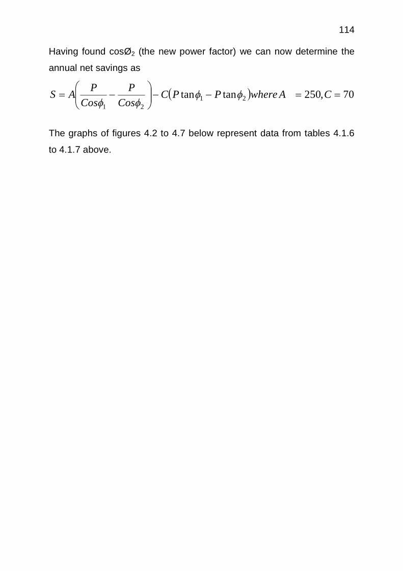
114 Having found cosØ2 (the new power factor) we can now determine the
annual net savings as
70,250tantan 2121
CAwherePPC
CosP
CosPAS
The graphs of figures 4.2 to 4.7 below represent data from tables 4.1.6
to 4.1.7 above.

115
0 500 1000 1500-50
0
50
100
150
200
250
Size of capacitor bank [KVar]
Pow
er L
oss
& L
oss
redu
ctio
n [K
w]
Power LossLoss reduction
Figure 4.2 Power loss & loss reduction versus size of capacitor bank on node 26 only
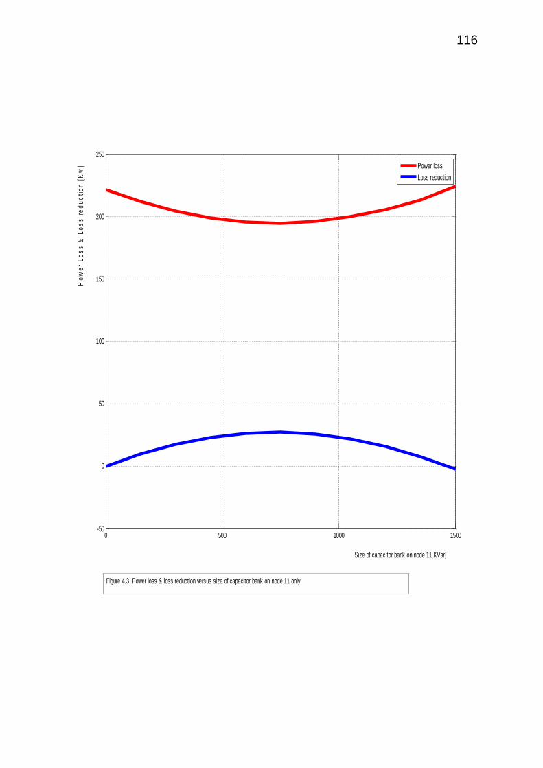
116
0 500 1000 1500-50
0
50
100
150
200
250
Size of capacitor bank on node 11[KVar]
Pow
er L
oss
& L
oss
redu
ctio
n [K
w]
Power lossLoss reduction
Figure 4.3 Power loss & loss reduction versus size of capacitor bank on node 11 only

117
600 800 1000 1200 1400 1600 1800 2000 2200 2400-50
0
50
100
150
200
250
Size of capacitor bank [KVar]
Pow
er L
oss
& L
oss
redu
ctio
n [K
w]
Power LossLoss reduction
Figure 4.4 Power loss & loss reduction versus total size of capacitor banks on nodes 26 &11

118
0 500 1000 15000
0.5
1
1.5
2
2.5
3
3.5
4x 10⁴
Size of capacitor bank on node 26[KVar]
Sav
ings
[N]
Figure 4.5 Savings per annum versus size of capacitor bank on node 26 only

119
0 500 1000 1500-8
-7
-6
-5
-4
-3
-2
-1
0
1
2x 10⁴
Size of capacitor bank on node 11[KVar]
Sav
ings
[N]
Figure 4.6 Savings per annum versus size of capacitor bank on node 11 only
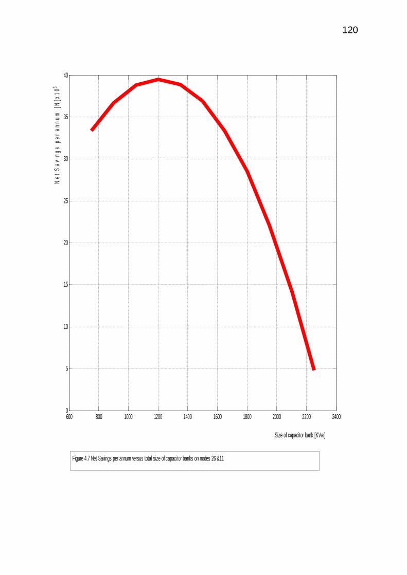
120
600 800 1000 1200 1400 1600 1800 2000 2200 24000
5
10
15
20
25
30
35
40
Size of capacitor bank [KVar]
Net
Sav
ings
per
ann
um [N
]x10
3
Figure 4.7 Net Savings per annum versus total size of capacitor banks on nodes 26 &11
121 Figure 4.1 Shows 34 Bus 11kV distribution feeder line with lateral
branches.
Plot of figure 4.2 shows the power loss and loss reduction versus size of
capacitor bank placed on node 26 only.
Plot of figure 4.3 shows the power loss and loss reduction due to
capacitor bank placed on node 11 only.
Plot of figure 4.4 shows overall power loss and loss reduction due to
capacitor banks placed on both node 26 and node 11combined.
The data of figures 4.2, 4.3 and 4.4 are shown in table 4.1.6.
Plot of figure 4.5 shows the savings per annum due to capacitor bank
placed on node 26 only.
Plot of figure 4.6 shows the saving per annum due to capacitor bank
placed on node 11 only.
Plot of figure 4.7 shows the overall net savings due capacitor banks
placed on both node 26 and node 11combined.
The data for figures 4.5, 4.6, and 4.7 are shown in table 4.1.7.
We have also plotted the net savings against capacitor sizes on nodes
26 and 11 as shown in figure 4.7.From the graph of figure 4.2, it is
obvious that the optimum size capacitor bank required at node 26 is 750
Kvar. This is the capacitor bank size that produces minimum power loss
and maximum power loss reduction.
The steps we have taken for node 26 are repeated for node 11
which is the next most sensitive node. It is the most sensitive node on
the main feeder. In addition to the 750kvar capacitor bank on node 26,
varying sizes of capacitor bank is connected to node 11.
Finally, it can be deduced from the tables and graphs that the
optimum capacitor bank size to be allocated to node 26 and node 11 are
750kvar and 450kvar respectively. With this, maximum net savings of
N39,500 (Thirty Nine thousand five hundred Naira only) per annum is
obtained. Also, a peak power loss reduction of 49.4kw is attained as in

122 table 4.9 If loss reduction higher than this is sought after, the net saving
will decrease because the cost of compensating capacitors will exceed
the benefits gained from reducing the power losses.
The time taken to save the initial cost of the capacitor is
T = N
ZY *
= 12000 x 700
39,500
= 21.266yrs
Where
Y = Value of capacitor in Kvar
Z = Cost of capacitor per Kvar in Naira
V*Z = Total cost of installed capacitor in Naira
N = Net saving in Naira

123
CHAPTER FIVE
CONCLUSIONS AND RECOMMENDATIONS
5.0 CONCLUSIONS
The ability of utility (eg distribution system) to reduce technical
losses in its operation will provide enough revenue for future expansion,
upgrades and modernization. This will improve on reliability and security
of supply. Many utilities are faced with the crippling effect of power
losses (Technical) and are putting in place various measures to reduce
these losses.
This project therefore presents a technique for reducing the power
losses arising from the flow of reactive power in a distribution system by
placing compensating capacitors at a few specific locations in the
network termed “sensitive nodes” to achieve a maximum loss reduction
and maximum annual naira savings. This method is applied to a 3-
phase, 11kv, 50HZ distribution network in Enugu.
Heuristic techniques are applied in this project to determine the
optimal capacitor placement and ratings for the distribution system.
This is achieved by examining the solution at a set of critical nodes
termed sensitive nodes. The sensitive nodes are selected based on the
losses caused in the system by the reactive components of the load
current. It is at these sensitive nodes that sizeable capacitor banks were
installed to achieve the desired high loss reduction in Enugu distribution
system.
5.1 RECOMMENDATIONS.
(i) Power Holding Company of Nigeria (PHCN) should take a
critical look at transformer loadings. Chiefs and political leaders
should be involved so that swapping of transformers could be
employed to limit overloading of transformers. Transformer
loading data from PHCN show that some transformers are

124
overloaded while others are far under utilized. Swapping of
transformers can be very involving but loadings of some
transformers are too high that they are threatened with eminent
destruction.
(ii) Attempts should be made at balancing the various phases of
loads since some imbalance has been observed on some
transformers.
(iii) A reappraisal should be done on the suitability of LV cables/
conductors and the needed upgrades carried out where
necessary. At some areas, the conductor sags are very severe
as a result of conductor heating and in order to prevent phase
conductors from clashing, they are held apart by spacers.
(iv) The low voltages as stated earlier are due to the system wide
low voltages. The prudent use tap changers or booster
transformers on bulk supply and distribution transformer should
be explored. It will be necessary that PHCN should conduct a
study on the use of compensating capacitors within the power
holding areas.
(v) Loss reduction units should step up their activities at the various
areas and check losses within their areas. It is recommended
that units could be rotated from time to time to stem the cases
of acquaintances with the customers.
(vi) Right technical decisions should be taken in sizing transformers
and cables in order to reduce technical losses. This should start
from planning phase and should be based on sound data to
accommodate future population increase and movement.
(vii) Finally, since power factor less than 0.9 in-cure a penalty, it is
therefore usually in the best financial interest of the industrial
customers of PHCN in Enugu to perform power factor correction
using shunt capacitors.
125
(viii) The capacitors retain electrical charge, even when the power is
switched off. It may be dangerous to touch the terminals of the
capacitors, unless the capacitors are fully discharged. For
safety requirements, all AMBER lighting capacitors are supplied
with internal discharge resistors, so that the capacitor voltage
drops to below 50 V within 1 minute of switch off. Even then,
care should be exercised in handling the lighting fixtures.
(ix) As ballasts generate heat, capacitors with thermoplastic cases
should be placed as much away from the ballasts as possible.
Care should be taken that the capacitor case temperature does
not exceed the rated temperature printed on the capacitor. If the
heat dissipation within the luminaire is not proper, capacitors
with aluminium case should be used.
(x) High efficiency transformers should be installed during the initial
installation of distribution system.

126
REFERENCES.
[1] Theraja, B.L., and Theraja, A.K. "A text book of electrical
technology twenty-second edition 1997 Ramngar, New Delhi"
[2] Sun, D.I.H., Abe S; Shoults R.R., Chen M.S., Eichenberger, P.,
Farris D. “Calculation of Energy Losses in a Distribution System,
“IEEE Transactions on Power Apparatus and Systems, V. 6,
PA5-99, No. 4, Jul. 1980.
[3] Gross, C.A., Power System Analysis, 2nd ed., 1986
[4] Nasar, S.A., Electric Energy Conservation and Transmission,
1986
[5] Chen, T.H., Chen, M.S., Inoue, T., Kotas P., Chebli, E.A., “Three
Phase Cogenerator and Transformer Models for Distribution
System Analysis,” IEEE Transactions on Power Delivery, V. 6, No.
4, Oct. 1991.
[6] Makino, A., Suzuki, K., Inoue, A., Masumoto, T., “Low Core Loss
of a bcc Fe86Zr7B6CUI Alloy with Nanoscale Grain Size, “Materials
Transactions, JIM (Japan Institute of Metals), V. 32, No. 6, Jun.
1991.
[7] Ng, H.W., Hasegawa, R., Lee, A.C.., Lowdermilk, L.A.,
“Amorphous Alloy Core Distribution Transformers,” IEEE
Proceedings, V. 79, No. 11, Nov. 1991
[8] Kerszenbauru, I; Mazur, A. Mistry, M., Frank J; “Specifying Dry-
Type Distribution Transformers for Solid-State Applications, “IEEE
Transactions on Industry Application, V. 27, No. 1, Jan. 1991.
[9] Abotsi, F., Bayor, R.K. and Amuna, W. "Loss reduction
strategies for Volta river authority (VRA)-Northern Electricity
Department (NED). 6Th International conference on power systems
operation and planning. Conference proceedings, may 22nd -26th,
2005, Universide Jean Piaget, Praia, Cape Verde.

127 [10] Sun. D.I.H, Abe. S.A. Shouts. R.R, M.S. Chen. Berger Eichea P.
and Farris. D. Calculation of energy losses in distribution systems.
IEEE Transaction on power apparatus and systems Vol. PAS-99,
NO4, JULY/.AUG. 1980. pp 1347-1356
[11] Lee R. E. and Brook C.L. "A method and its application to
evaluate automated distribution control. IEEE Transaction on
power delivery Vol. 3 No 3, July 1988. pp 1232-1240
[12] Chis, M., Salama, M.M.A. and Ayaram, S.J. “Capacitor
placement in distribution system using heuristic search strategies”,
IEE Proc. Transm. Distribution. Vol. 144, No. 3, May 1997.
pp 225-230
[13] Bae, Y.G. “Analytical Method of capacitor allocation on
distribution primary feeders”, IEEE Transaction on Power
Apparatus and System. Vol. PAS-97, No. 4 July/Aug. 1978.
1232 - 1238
[14] Change , N.E. “Generalized equation on loss reduction with
shunt capacitors” IEEE Trans, PAS-91, SEPT./OCT. 1992
pp. 2189-2195
[15] Grainger, J.J. and LEE, S.H. “Optimum size and location of shunt
capacitors for reduction of losses on distribution system”, IEEE
Transaction PAS-100, 1981. pp 1105-1118
[16] Lee, S.H. and Grainger, J.J. “Optimum placement of fixed and
switched capacitors on primary distribution feeders” IEEE Trans.
PAS-100, 1981. pp 345-352
[17] Salama, M.M.A. and Chikhani, A.Y., “A simplified network
approach to VArs control problem for radial distribution system,
IEEE. Trans. Power Delivery, 1993, 8, (3), pp. 1529-1535.
[18] Kalyuzhny, A; Levitin, G. Elmakis, D. and Ben-Halm, H. “System
approach to shunt capacitor allocation in radial distribution systems”

128
Electric Power System Research, Volume 56, Issue 1, 5 October 2000,
pp. 51-60.
[19] Fariz Tharwat, H., El-Sobki Salah, M. and Abdel-Halim Mohamed .A.
“New approach for the application of shunt capacitors to the
primary distribution feeders. IEEE Transactions on Power
apparatus and systems, Vol. PAS-102, No. 1, January 1983
pp. 10-13
[20] Abdel-Salam, T.S., Chikhani, A.Y., and Hackam, R. “A new
techniques for loss reduction using compensating capacitors
applied to distribution systems with varying load condition,” IEEE
Trans. Power Delivery, 1994, Vol. 9 No. (2) pp 819-827
[21] Salama, M.M.A., Chikhani, A.Y. and Hackam, R. “Control of
Reactive Power in Distribution System with an End load and Fixed
Load Condition”, IEEE Trans. Vol. PAS-104, 1985. pp 2779-2788
[22] Salama, M.M.A, Mansour, E.A.A., Chikhani, A.Y. and Hackam, R. “Control of Reactive Power in Distribution Systems with an End
Load and Varying Load Conditions”, IEEE Trans, Vol. Pas-104,
1985. pp 941-947
[23] Gonen, T. “Electric Power Distribution System Engineering”
McGraw-Hill, 1986.
[24] Donald Bee Man “Industrial Power System Handbook” First
Edition, 1955. McGraw-Hill Book Company Inc. New York, Toronto
London
[25] Moreli, Jordan. E. “Distribution Loss Reduction: A Genetic
Algorithm Approach”. A thesis for the degree of master of Applied
Science at the University of Windsor, Windsor, Ontario,
Canada, 1998.
[26] htt://en.wikipedia.org/wiki/Active-power-factor-correction
[27] http://ambercaps .com/lighting/powerfactor-correction-concepts.htm
[28] http://openbookproject.net/electricCircuits/AC/AC-//.html

129 [29] Htt://www.siemens.de/pr/inf/20/55/dooooooo.htm
[30] IEEE Guide For Application Of Shunt Capacitors IEEE std. 1036-1992
[31] www.jcmiras.net/jcm/item/77
[32] file://c//my%20Documents/electrical/power%20factor%20
correction.htm. (12 of 14)
[33] Francis, T.G. “Electrical Installation Work” Fifth Metric Low Priced
Edition, 1971
[34] http://www.wapedia.mobi/en/power-factor “then click: wapedia-
wiki:power factor”
[35] http://www.st.com/stonline/products/literatuyre/an/3727.htm, “then
click format 404kb”
[36] http://www.novation.com/Active power factor/techniques and solutions, part 3.
[37] Prasad, A.R.; Ziogas, P.D. and Manias, S. “An Active Power
Factor Correction Technique for Three-Phase Diode Rectifiers” IEE
Transaction on Power Electronics. Vol. 6., No. 1 January 1991. [38] www.tinitron.com
[39] http://www.geocities.com/solicomValley/Lab/4223/Pflow/bch01.htm.
[40] Stevenson, W.A. JR. “Elements of Power System analysis Fourth
Edition, 1982, McGraw-Hill Series in Electrical Engineering,
Singapore, Sydney, Tokyo, Toronto.
[41] Wagner, T.P., Chikhani, A.Y. and Hackam, R. “Feeder
Reconfiguration for Loss reduction: An application of distribution
Automation”, IEEE Transaction on Power Delivery Vol. 6, No. 4,
October, 1991, PP. 1922-1933, PP. 1922-1933.
[42] Symonds, A. “Electrical Power Equipment and Measurements:
with heavy current electrical applications” Second Edition, 1980.
McGraw-Hill Book Company (UK) Limited London, New York,
Singapore, Tokyo, Toronto.
[43] Ewesor, P.O. “Practical Electrical System Installation Work and
Practice” First Edition 2003.

130
APPENDIX I
SUMMARY OF RELEVANT FORMULAE
The distribution system under consideration is a concentrated
load.
1. Losses before addition of capacitor (table 4.1.5) is obtained from:
62.32
112
1112 equationRSinIRCosIRI
2. Losses after addition of capacitor (table 4.1.6) is obtained from:
63.3
211
2222
2 equationRIcSinIRCosIRI
3. Power loss reduction
68.3sin2 211 EquationfromobtainedisRIRIIL Cc
where I = current flowing through the circuit
R = Resistance
VQc
VK
equationSinISinIIc
var
58.32211
4. Capacitor size ratings are obtained from
02
01
21
26.16,79.31
81.23tantanvar
where
equationPK c
5. Optimal Economical power factor 0.96 2Cos is obtained from:
99.3......1100
11 22
22
2 equationSinA
BpACCos
6. Net Annual savings:
85.3...tantan 2121
equationfromobtainedisPPCCos
PCos
PAS

131
7. Considering the loss reduction based on the combination of active
and reactive components of current, the power loss becomes.
kw
rilririlaiii
riliIL
P
Mm
Li
6.221
222
= the initial peak power loss in the system.
(8) Formular for bus current is
jjjjj YVVI 11
Where j = 2, 3, 4…..
(9) Formular for power loses before addition of capacitor is
PLi = ii RI 23
Where i = 2, 3, 4…..
(10) Formular for power loses due to reactive component of current is
iri RILi 23Pr
Where I = 1,2,3…
(11) Formular for admittance of the sections are:
For self admittance: j
ij ZY 1
Where i = 1,2,..
J = 2,3…
For mutual admittance; Yii = Yi1 + Yi2 + Yi3
(12) Formular for load currents is
Ii = YjiVi - YijVj
Where I = 1,2,3
j = 2,3,4

132 (13) Formular for total power loss after compensation is
PL2 = (I2 + IC11 + IC26)2R2
PL 3 = (I3 + IC11 + IC26)2R3
PL 4 = (I4 + IC11 + IC26)2R4
PL 5 = (I5 + IC11 + IC26)2R5
PL 6 = (I6 + IC11 + IC26)2R6
PL 7 = (I7 + IC11)2R7
PL 8 = (I8 + IC11)2R8
PL 9 = (I9 + IC11)2R9
PL 10 = (I10 + IC11)2R10
PL 11 = (I11 + IC11)2R11
PL 17 = (I17 + IC26)2R17
PL 18 = (I18 + IC26)2R18
PL 19 = (I19 + IC26)2R19
PL 20 = (I20 + IC26)2R20
PL 21 = (I21 + IC26)2R21
PL 22 = (I22 + IC26)2R22
PL 23 = (I23 + IC26)2R23
PL 24 = (I24 + IC26)2R24
PL 25 = (I25 + IC26) 2R25
PL 26 = (I26 + IC26) 2R26
APPENDIX II

133
LOAD FLOW PROGRAMME IN MATLAB
A. % Base values
vb=11;
sb=100;
zb=vb^2/sb;
B. % BUS DATA
C. % Load per unit
s1=0;
s2=(-230-142.5i)/100000;
s3=0;
s4=s2;
s5=s4;
s6=0;
s7=0;
s8=s5;
s9=s8;
s10=0;
s11=s9;
s12=(-137-84i)/100000;
s13=(-72-45i)/100000;
s14=s13;
s15=s14;
s16=(-13.5-7.5i)/100000;
s17=s11;
s18=s17;
s19=s18;
s20=s19;

134
s21=s20;
s22=s21;
s23=s22;
s24=s23;
s25=s24;
s26=s25;
s27=(-137-85i)/100000;
s28=(-75-48i)/100000;
s29=s28;
s30=s29;
s31=(-57-34.5i)/100000;
s32=s31;
s33=s32;
s34=s33;
D. % Voltage
v1=1.00;
v2=1.00;
v3=1.00;
v4=1.00;
v5=1.00;
v6=1.00;
v7=1.00;
v8=1.00;
v9=1.00;
v10=1.00;
v11=1.00;
v12=1.00;
v13=1.00;
v14=1.00;

135
v15=1.00;
v16=1.00;
v17=1.00;
v18=1.00;
v19=1.00;
v20=1.00;
v21=1.00;
v22=1.00;
v23=1.00;
v24=1.00;
v25=1.00;
v26=1.00;
v27=1.00;
v28=1.00;
v29=1.00;
v30=1.00;
v31=1.00;
v32=1.00;
v33=1.00;
v34=1.00;
LINE DATA
E. % Line Impedance per unit
z2=0.6*(0.195+0.080i)/zb;
z3=0.55*(0.195+0.080i)/zb;
z4=0.55*(0.299+0.083i)/zb;
z5=0.50*(0.299+0.083i)/zb;
z6=z5;
z7=0.60*(0.524+0.090i)/zb;
z8=0.40*(0.524+0.090i)/zb;

136
z9=z7;
z10=z8;
z11=0.25*(0.524+0.090i)/zb;
z12=0.20*(0.524+0.090i)/zb;
z13=0.30*(0.524+0.090i)/zb;
z14=z10;
z15=z12;
z16=0.10*(0.524+0.090i)/zb;
z17=0.60*(0.299+0.083i)/zb;
z18=z4;
z19=0.55*(0.378+0.086i)/zb;
z20=0.50*(0.378+0.086i)/zb;
z21=z20;
z22=0.50*(0.524+0.090i)/zb;
z23=z22;
z24=z9;
z25=z14;
z26=z11;
z27=z15;
z28=z13;
z29=z28;
z30=z29;
z31=z30;
z32=z25;
z33=z31;
z34=z27;
F. % Line admittances

137
y12=1/z2;
y21=y12;
y23=1/z3;
y32=y23;
y34=1/z4;
y43=y34;
y45=1/z5;
y54=y45;
y56=1/z6;
y65=y56;
y67=1/z7;
y76=y67;
y78=1/z8;
y87=y78;
y89=1/z9;
y98=y89;
y910=1/z10;
y109=y910;
y1011=1/z11;
y1110=y1011;
y1112=1/z12;
y1211=y1112;
y313=1/z13;
y133=y313;
y1314=1/z14;
y1413=y1314;
y1415=1/z15;
y1514=y1415;
y1516=1/z16;
y1615=y1516;
138
y617=1/z17;
y176=y617;
y1718=1/z18;
y1817=y1718;
y1819=1/z19;
y1918=y1819;
y1920=1/z20;
y2019=y1920;
y2021=1/z21;
y2120=y2021;
y2122=1/z22;
y2221=y2122;
y2223=1/z23;
y2322=y2223;
y2324=1/z24;
y2423=y2324;
y2425=1/z25;
y2524=y2425;
y2526=1/z26;
y2625=y2526;
y2627=1/z27;
y2726=y2627;
y728=1/z28;
y287=y728;
y2829=1/z29;
y2928=y2829;
y2930=1/z30;
y3029=y2930;
y1031=1/z31;
y3110=y1031;

139
y3132=1/z32;
y3231=y3132;
y3233=1/z33;
y3332=y3233;
y3334=1/z34;
y3433=y3334;
y22=y21+y23;
y33=y32+y34+y313;
y44=y43+y45;
y55=y54+y56;
y66=y65+y67+y617;
y77=y76+y78+y728;
y88=y87+y89;
y99=y98+y910;
y1010=y109+y1011+y1031;
y1111=y1110+y1112;
y1212=y1211;
y1313=y133+y1314;
y1414=y1413+y1415;
y1515=y1514+y1516;
y1616=y1615;
y1717=y176+y1718;
y1818=y1817+y1819;
y1919=y1918+y1920;
y2020=y2019+y2021;
y2121=y2120+y2122;
y2222=y2221+y2223;
y2323=y2322+y2324;
y2424=y2423+y2425;
y2525=y2524+y2526;

140
y2626=y2625+y2627;
y2727=y2726;
y2828=y287+y2829;
y2929=y2928+y2930;
y3030=y3029;
y3131=y3110+y3132;
y3232=y3231+y3233;
y3333=y3332+y3334;
y3434=y3433;
G. % Computation of bus voltages
k=1;
v22(k)=1/y22*(conj(s2/v2)+y21*v1+y23*v3);
v2(k)=v2+1.6*(v22(k)-v2);
v33(k)=1/y33*(conj(s3/v3)+y32*v2(k)+y313*v13+y34*v4);
v3(k)=v3+1.6*(v33(k)-v3);
v44(k)=1/y44*(conj(s4/v4)+y43*v3(k)+y45*v5);
v4(k)=v4+1.6*(v44(k)-v4);
v55(k)=1/y55*(conj(s5/v5)+y54*v4(k)+y56*v6);
v5(k)=v5+1.6*(v55(k)-v5);
v66(k)=1/y66*(conj(s6/v6)+y65*v5(k)+y67*v7+y617*v17);
v6(k)=v6+1.6*(v66(k)-v6);
v77(k)=1/y77*(conj(s7/v7)+y76*v6(k)+y78*v8+y728*v28);
v7(k)=v7+1.6*(v77(k)-v7);
v88(k)=1/y88*(conj(s8/v8)+y87*v7(k)+y89*v9);
v8(k)=v8+1.6*(v88(k)-v8);
v99(k)=1/y99*(conj(s9/v9)+y98*v8(k)+y910*v10);
v9(k)=v9+1.6*(v99(k)-v9);
v1010=1/y1010*(conj(s10/v10)+y109*v9(k)+y1011*v11+y1031*v31);
v10(k)=v10+1.6*(v1010(k)-v10);
v1111(k)=1/y1111*(conj(s11/v11)+y1110*v10(k)+y1112*v12);

141
v11(k)=v11+1.6*(v1111(k)-v11);
v1212(k)=1/y1212*(conj(s12/v12)+y1211*v11(k));
v12(k)=v12+1.6*(v1212(k)-v12);
v1313(k)=1/y1313*(conj(s13/v13)+y133*v3(k)+y1314*v14);
v13(k)=v13+1.6*(v1313(k)-v13);
v1414(k)=1/y1414*(conj(s14/v14)+y1413*v13(k)+y1415*v15);
v14(k)=v14+1.6*(v1414(k)-v14);
v1515(k)=1/y1515*(conj(s15/v15)+y1514*v14(k)+y1516*v16);
v15(k)=v15+1.6*(v1515(k)-v15);
v1616(k)=1/y1616*(conj(s16/v16)+y1615*v15(k));
v16(k)=v16+1.6*(v1616(k)-v16);
v1717(k)=1/y1717*(conj(s17/v17)+y176*v6(k)+y1718*v18);
v17(k)=v17+1.6*(v1717(k)-v17);
v1818(k)=1/y1818*(conj(s18/v18)+y1817*v17(k)+y1819*v19);
v18(k)=v18+1.6*(v1818(k)-v18);
v1919(k)=1/y1919*(conj(s19/v19)+y1918*v18(k)+y1920*v20);
v19(k)=v19+1.6*(v1919(k)-v19);
v2020=1/y2020*(conj(s20/v20)+y2019*v19(k)+y2021*v21);
v20(k)=v20+1.6*(v2020(k)-v20);
v2121(k)=1/y2121*(conj(s21/v21)+y2120*v20(k)+y2122*v22);
v21(k)=v21+1.6*(v2121(k)-v21);
v2222(k)=1/y2222*(conj(s22/v22)+y2221*v21(k)+y2223*v23);
v22(k)=v22+1.6*(v2222(k)-v22);
v2323(k)=1/y2323*(conj(s23/v23)+y2322*v22(k)+y2324*v24);
v23(k)=v23+1.6*(v2323(k)-v23);
v2424(k)=1/y2424*(conj(s24/v24)+y2423*v23(k)+y2425*v25);
v24(k)=v24+1.6*(v2424(k)-v24);
v2525(k)=1/y2525*(conj(s25/v25)+y2524*v24(k)+y2526*v26);
v25(k)=v25+1.6*(v2525(k)-v25);
v2626(k)=1/y2626*(conj(s26/v26)+y2625*v25(k)+y2627*v27);
v26(k)=v26+1.6*(v2626(k)-v26);
v2727(k)=1/y2727*(conj(s27/v27)+y2726*v26(k));

142
v27(k)=v27+1.6*(v2727(k)-v27);
v2828(k)=1/y2828*(conj(s28/v28)+y287*v7(k)+y2829*v29);
v28(k)=v28+1.6*(v2828(k)-v28);
v2929(k)=1/y2929*(conj(s29/v29)+y2928*v28(k)+y2930*v30);
v29(k)=v29+1.6*(v2929(k)-v29);
v3030=1/y3030*(conj(s30/v30)+y3029*v29(k));
v30(k)=v30+1.6*(v3030(k)-v30);
v3131(k)=1/y3131*(conj(s31/v31)+y3110*v10(k)+y3132*v32);
v31(k)=v31+1.6*(v3131(k)-v31);
v3232(k)=1/y3232*(conj(s32/v32)+y3231*v31(k)+y3233*v33);
v32(k)=v32+1.6*(v3232(k)-v32);
v3333(k)=1/y3333*(conj(s33/v33)+y3332*v32(k)+y3334*v34);
v33(k)=v33+1.6*(v3333(k)-v33);
v3434(k)=1/y3434*(conj(s34/v34)+y3433*v33(k));
v34(k)=v34+1.6*(v3434(k)-v34);
for k=2:1:400;
v22(k)=1/y22*(conj(s2/v2(k-1))+y21*v1+y23*v3(k-1));
v2(k)=v2(k-1)+1.6*(v22(k)-v2(k-1));
v33(k)=1/y33*(conj(s3/v3(k-1))+y32*v2(k)+y313*v13(k-1)+y34*v4(k-1));
v3(k)=v3(k-1)+1.6*(v33(k)-v3(k-1));
v44(k)=1/y44*(conj(s4/v4(k-1))+y43*v3(k)+y45*v5(k-1));
v4(k)=v4(k-1)+1.6*(v44(k)-v4(k-1));
v55(k)=1/y55*(conj(s5/v5(k-1))+y54*v4(k)+y56*v6(k-1));
v5(k)=v5(k-1)+1.6*(v55(k)-v5(k-1));
v66(k)=1/y66*(conj(s6/v6(k-1))+y65*v5(k)+y67*v7(k-1)+y617*v17(k-1));
v6(k)=v6(k-1)+1.6*(v66(k)-v6(k-1));
v77(k)=1/y77*(conj(s7/v7(k-1))+y76*v6(k)+y78*v8(k-1)+y728*v28(k-1));
v7(k)=v7(k-1)+1.6*(v77(k)-v7(k-1));
v88(k)=1/y88*(conj(s8/v8(k-1))+y87*v7(k)+y89*v9(k-1));
v8(k)=v8(k-1)+1.6*(v88(k)-v8(k-1));
v99(k)=1/y99*(conj(s9/v9(k-1))+y98*v8(k)+y910*v10(k-1));
143
v9(k)=v9(k-1)+1.6*(v99(k)-v9(k-1));
v1010(k)=1/y1010*(conj(s10/v10(k-1))+y109*v9(k)+y1011*v11(k-
1)+y1031*v31(k-1));
v10(k)=v10(k-1)+1.6*(v1010(k)-v10(k-1));
v1111(k)=1/y1111*(conj(s11/v11(k-1))+y1110*v10(k)+y1112*v12(k-1));
v11(k)=v11(k-1)+1.6*(v1111(k)-v11(k-1));
v1212(k)=1/y1212*(conj(s12/v12(k-1))+y1211*v11(k));
v12(k)=v12(k-1)+1.6*(v1212(k)-v12(k-1));
v1313(k)=1/y1313*(conj(s13/v13(k-1))+y133*v3(k)+y1314*v14(k-1));
v13(k)=v13(k-1)+1.6*(v1313(k)-v13(k-1));
v1414(k)=1/y1414*(conj(s14/v14(k-1))+y1413*v13(k)+y1415*v15(k-1));
v14(k)=v14(k-1)+1.6*(v1414(k)-v14(k-1));
v1515(k)=1/y1515*(conj(s15/v15(k-1))+y1514*v14(k)+y1516*v16(k-1));
v15(k)=v15(k-1)+1.6*(v1515(k)-v15(k-1));
v1616(k)=1/y1616*(conj(s16/v16(k-1))+y1615*v15(k));
v16(k)=v16(k-1)+1.6*(v1616(k)-v16(k-1));
v1717(k)=1/y1717*(conj(s17/v17(k-1))+y176*v6(k)+y1718*v18(k-1));
v17(k)=v17(k-1)+1.6*(v1717(k)-v17(k-1));
v1818(k)=1/y1818*(conj(s18/v18(k-1))+y1817*v17(k)+y1819*v19(k-1));
v18(k)=v18(k-1)+1.6*(v1818(k)-v18(k-1));
v1919(k)=1/y1919*(conj(s19/v19(k-1))+y1918*v18(k)+y1920*v20(k-1));
v19(k)=v19(k-1)+1.6*(v1919(k)-v19(k-1));
v2020(k)=1/y2020*(conj(s20/v20(k-1))+y2019*v19(k)+y2021*v21(k-1));
v20(k)=v20(k-1)+1.6*(v2020(k)-v20(k-1));
v2121(k)=1/y2121*(conj(s21/v21(k-1))+y2120*v20(k)+y2122*v22(k-1));
v21(k)=v21(k-1)+1.6*(v2121(k)-v21(k-1));
v2222(k)=1/y2222*(conj(s22/v22(k-1))+y2221*v21(k)+y2223*v23(k-1));
v22(k)=v22(k-1)+1.6*(v2222(k)-v22(k-1));
v2323(k)=1/y2323*(conj(s23/v23(k-1))+y2322*v22(k)+y2324*v24(k-1));
v23(k)=v23(k-1)+1.6*(v2323(k)-v23(k-1));
v2424(k)=1/y2424*(conj(s24/v24(k-1))+y2423*v23(k)+y2425*v25(k-1));
v24(k)=v24(k-1)+1.6*(v2424(k)-v24(k-1));

144
v2525(k)=1/y2525*(conj(s25/v25(k-1))+y2524*v24(k)+y2526*v26(k-1));
v25(k)=v25(k-1)+1.6*(v2525(k)-v25(k-1));
v2626(k)=1/y2626*(conj(s26/v26(k-1))+y2625*v25(k)+y2627*v27(k-1));
v26(k)=v26(k-1)+1.6*(v2626(k)-v26(k-1));
v2727(k)=1/y2727*(conj(s27/v27(k-1))+y2726*v26(k));
v27(k)=v27(k-1)+1.6*(v2727(k)-v27(k-1));
v2828(k)=1/y2828*(conj(s28/v28(k-1))+y287*v7(k)+y2829*v29(k-1));
v28(k)=v28(k-1)+1.6*(v2828(k)-v28(k-1));
v2929(k)=1/y2929*(conj(s29/v29(k-1))+y2928*v28(k)+y2930*v30(k-1));
v29(k)=v29(k-1)+1.6*(v2929(k)-v29(k-1));
v3030(k)=1/y3030*(conj(s30/v30(k-1))+y3029*v29(k));
v30(k)=v30(k-1)+1.6*(v3030(k)-v30(k-1));
v3131(k)=1/y3131*(conj(s31/v31(k-1))+y3110*v10(k)+y3132*v32(k-1));
v31(k)=v31(k-1)+1.6*(v3131(k)-v31(k-1));
v3232(k)=1/y3232*(conj(s32/v32(k-1))+y3231*v31(k)+y3233*v33(k-1));
v32(k)=v32(k-1)+1.6*(v3232(k)-v32(k-1));
v3333(k)=1/y3333*(conj(s33/v33(k-1))+y3332*v32(k)+y3334*v34(k-1));
v33(k)=v33(k-1)+1.6*(v3333(k)-v33(k-1));
v3434(k)=1/y3434*(conj(s34/v34(k-1))+y3433*v33(k));
v34(k)=v34(k-1)+1.6*(v3434(k)-v34(k-1));
end
v1=1.00;
v2=v2(400);
V2=abs(v2)*11000;
v3=v3(400);
V3=abs(v3)*11000;
v4=v4(400);
V4=abs(v4)*11000;
v5=v5(400);
V5=abs(v5)*11000;
v6=v6(400);

145
V6=abs(v6)*11000;
v7=v7(400);
V7=abs(v7)*11000;
v8=v8(400);
V8=abs(v8)*11000;
v9=v9(400);
V9=abs(v9)*11000;
v10=v10(400);
V10=abs(v10)*11000;
v11=v11(400);
V11=abs(v11)*11000;
v12=v12(400);
V12=abs(v12)*11000;
v13=v13(400);
V13=abs(v13)*11000;
v14=v14(400);
V14=abs(v14)*11000;
v15=v15(400);
V15=abs(v15)*11000;
v16=v16(400);
V16=abs(v16)*11000;
v17=v17(400);
V17=abs(v17)*11000;
v18=v18(400);
V18=abs(v18)*11000;
v19=v19(400);
V19=abs(v19)*11000;
v20=v20(400);
V20=abs(v20)*11000;
v21=v21(400);
V21=abs(v21)*11000;
v22=v22(400);

146
V22=abs(v22)*11000;
v23=v23(400);
V23=abs(v23)*11000;
v24=v24(400);
V24=abs(v24)*11000;
v25=v25(400);
V25=abs(v25)*11000;
v26=v26(400);
V26=abs(v26)*11000;
v27=v27(400);
V27=abs(v27)*11000;
v28=v28(400);
V28=abs(v28)*11000;
v29=v29(400);
V29=abs(v29)*11000;
v30=v30(400);
V30=abs(v30)*11000;
v31=v31(400);
V31=abs(v31)*11000;
v32=v32(400);
V32=abs(v32)*11000;
v33=v33(400);
V33=abs(v33)*11000;
v34=v34(400);
V34=abs(v34)*11000;
H. % Line Currents
ib=100000/((sqrt(3)*11));
i2=(v1-v2)*y12*ib;
i3=(v2-v3)*y23*ib;
i4=(v3-v4)*y34*ib;
147
i5=(v4-v5)*y45*ib;
i6=(v5-v6)*y56*ib;
i7=(v6-v7)*y67*ib;
i8=(v7-v8)*y78*ib;
i9=(v8-v9)*y89*ib;
i10=(v9-v10)*y910*ib;
i11=(v10-v11)*y1011*ib;
i12=(v11-v12)*y1112*ib;
i13=(v3-v13)*y313*ib;
i14=(v13-v14)*y1314*ib;
i15=(v14-v15)*y1415*ib;
i16=(v15-v16)*y1516*ib;
i17=(v6-v17)*y617*ib;
i18=(v17-v18)*y1718*ib;
i19=(v18-v19)*y1819*ib;
i20=(v19-v20)*y1920*ib;
i21=(v20-v21)*y2021*ib;
i22=(v21-v22)*y2122*ib;
i23=(v22-v23)*y2223*ib;
i24=(v23-v24)*y2324*ib;
i25=(v24-v25)*y2425*ib;
i26=(v25-v26)*y2526*ib;
i27=(v26-v27)*y2627*ib;
i28=(v7-v28)*y728*ib;
i29=(v28-v29)*y2829*ib;
i30=(v29-v30)*y2930*ib;
i31=(v10-v31)*y1031*ib;
i32=(v31-v32)*y3132*ib;
i33=(v32-v33)*y3233*ib;
i34=(v33-v34)*y3334*ib;

148 I. % Calculation of Losses
pl2=3*(i2)^2*real(z2)*zb;
pl3=3*(i3)^2*real(z3)*zb;
pl4=3*(i4)^2*real(z4)*zb;
prl=3*(i5)^2*real(z5)*zb;
pl6=3*(i6)^2*real(z6)*zb;
pl7=3*(i7)^2*real(z7)*zb;
pl8=3*(i8)^2*real(z8)*zb;
pl9=3*(i9)^2*real(z9)*zb;
pl10=3*(i10)^2*real(z10)*zb;
pl11=3*(i11)^2*real(z11)*zb;
pl12=3*(i12)^2*real(z12)*zb;
pl13=3*(i13)^2*real(z13)*zb;
pl14=3*(i14)^2*real(z14)*zb;
pl15=3*(i15)^2*real(z15)*zb;
pl16=3*(i16)^2*real(z16)*zb;
pl17=3*(i17)^2*real(z17)*zb;
pl18=3*(i18)^2*real(z18)*zb;
pl19=3*(i19)^2*real(z19)*zb;
pl20=3*(i20)^2*real(z20)*zb;
pl21=3*(i21)^2*real(z21)*zb;
pl22=3*(i22)^2*real(z22)*zb;
pl23=3*(i23)^2*real(z23)*zb;
pl24=3*(i24)^2*real(z24)*zb;
pl25=3*(i25)^2*real(z25)*zb;
pl26=3*(i26)^2*real(z26)*zb;
pl27=3*(i27)^2*real(z27)*zb;
pl28=3*(i28)^2*real(z28)*zb;
pl29=3*(i29)^2*real(z29)*zb;
pl30=3*(i30)^2*real(z30)*zb;
149
pl31=3*(i31)^2*real(z31)*zb;
pl32=3*(i32)^2*real(z32)*zb;
pl33=3*(i33)^2*real(z33)*zb;
pl34=3*(i34)^2*real(z34)*zb;
plt=pl2+pl3+pl4+pl5+pl6+pl7+pl8+pl9+pl10+pl11+pl12+pl13+pl14+
pl15+pl16+pl17+pl18+pl19+pl20+pl21+pl22+pl23+pl24+pl25+pl26
+pl27+pl28+pl29+pl30+pl31+pl32+pl33+pl34;
plt=221.71
J. % Losses due to active components of current
pa2=3*(real(i2))^2*real(z2)*zb/1000
pa3=3*(real(i3))^2*real(z3)*zb/1000
pa4=3*(real(i4))^2*real(z4)*zb/1000
pa5=3*(real(i5))^2*real(z5)*zb/1000
pa6=3*(real(i6))^2*real(z6)*zb/1000
pa7=3*(real(i7))^2*real(z7)*zb/1000
pa8=3*(real(i8))^2*real(z8)*zb/1000
pa9=3*(real(i9))^2*real(z9)*zb/1000
pa10=3*(real(i10))^2*real(z10)*zb/1000
pa11=3*(real(i11))^2*real(z11)*zb/1000
pa12=3*(real(i12))^2*real(z12)*zb/1000
pa13=3*(real(i13))^2*real(z13)*zb/1000
pa14=3*(real(i14))^2*real(z14)*zb/1000
pa15=3*(real(i15))^2*real(z15)*zb/1000
pa16=3*(real(i16))^2*real(z16)*zb/1000
pa17=3*(real(i17))^2*real(z17)*zb/1000
pa18=3*(real(i18))^2*real(z18)*zb/1000
pa19=3*(real(i19))^2*real(z19)*zb/1000
pa20=3*(real(i20))^2*real(z20)*zb/1000

150
pa21=3*(real(i21))^2*real(z21)*zb/1000
pa22=3*(real(i22))^2*real(z22)*zb/1000
pa23=3*(real(i23))^2*real(z23)*zb/1000
pa24=3*(real(i24))^2*real(z24)*zb/1000
pa25=3*(real(i25))^2*real(z25)*zb/1000
pa26=3*(real(i26))^2*real(z26)*zb/1000
pa27=3*(real(i27))^2*real(z27)*zb/1000
pa28=3*(real(i28))^2*real(z28)*zb/1000
pa29=3*(real(i29))^2*real(z29)*zb/1000
pa30=3*(real(i30))^2*real(z30)*zb/1000
pa31=3*(real(i31))^2*real(z31)*zb/1000
pa32=3*(real(i32))^2*real(z32)*zb/1000
pa33=3*(real(i33))^2*real(z33)*zb/1000
pa34=3*(real(i34))^2*real(z34)*zb/1000
K. % Losses due to reactive components of current
pr2=3*(imag(i2))^2*real(z2)*zb/1000
pr3=3*(imag(i3))^2*real(z3)*zb/1000
pr4=3*(imag(i4))^2*real(z4)*zb/1000
pr5=3*(imag(i5))^2*real(z5)*zb/1000
pr6=3*(imag(i6))^2*real(z6)*zb/1000
pr7=3*(imag(i7))^2*real(z7)*zb/1000
pr8=3*(imag(i8))^2*real(z8)*zb/1000
pr9=3*(imag(i9))^2*real(z9)*zb/1000
pr10=3*(imag(i10))^2*real(z10)*zb/1000
pr11=3*(imag(i11))^2*real(z11)*zb/1000
pr12=3*(imag(i12))^2*real(z12)*zb/1000
pr13=3*(imag(i13))^2*real(z13)*zb/1000
pr14=3*(imag(i14))^2*real(z14)*zb/1000
pr15=3*(imag(i15))^2*real(z15)*zb/1000

151
pr16=3*(imag(i16))^2*real(z16)*zb/1000
pr17=3*(imag(i17))^2*real(z17)*zb/1000
pr18=3*(imag(i18))^2*real(z18)*zb/1000
pr19=3*(imag(i19))^2*real(z19)*zb/1000
pr20=3*(imag(i20))^2*real(z20)*zb/1000
pr21=3*(imag(i21))^2*real(z21)*zb/1000
pr22=3*(imag(i22))^2*real(z22)*zb/1000
pr23=3*(imag(i23))^2*real(z23)*zb/1000
pr24=3*(imag(i24))^2*real(z24)*zb/1000
pr25=3*(imag(i25))^2*real(z25)*zb/1000
pr26=3*(imag(i26))^2*real(z26)*zb/1000
pr27=3*(imag(i27))^2*real(z27)*zb/1000
pr28=3*(imag(i28))^2*real(z28)*zb/1000
pr29=3*(imag(i29))^2*real(z29)*zb/1000
pr30=3*(imag(i30))^2*real(z30)*zb/1000
pr31=3*(imag(i31))^2*real(z31)*zb/1000
pr32=3*(imag(i32))^2*real(z32)*zb/1000
pr33=3*(imag(i33))^2*real(z33)*zb/1000
pr34=3*(imag(i34))^2*real(z34)*zb/1000
prt=pr2+pr3+pr4+pr5+pr6+pr7+pr8+pr9+pr10+pr11+pr12+pr13+pr
14+pr15+pr16+pr17+pr18+pr19+pr20+pr21+pr22+pr23+pr24+pr25
+pr26+pr27+pr28+pr29+pr30+pr31+pr32+pr33+pr34;
L. % Load Currents
il2 = conj
2
2
VS
il4 = conj
4
4
VS

152
il5 = conj
5
5
VS
il8 = conj
8
8
VS
il9=il8;
il11=il9;
il12 = conj
12
12
VS
il13 = conj
13
13
VS
il14=il13;
il15=il14;
il16 = conj
16
16
VS
il17=il11;
il18=il17;
il19=il18;
il20=il19;
il21=il20;
il22=il21;
il23=il22;
il24=il23;
il25=il24;
il26=il25;
il27=il12;
il28 = conj
28
28
VS
il29=il28;
il30=il29;

153
il31 = conj
31
31
VS
il32=il31;
il33=il32;
il34=il33;
M. % Losses due to reactive component of load currents
l2=(imag(il2))^2*0.117;
l4=(imag(il4))^2*0.3887;
l5=(imag(il5))^2*0.5382;
l8=(imag(il8))^2*1.2117;
l9=(imag(il9))^2*1.5261;
l11=(imag(il11))^2*1.8667;
l12=(imag(il12))^2*1.9715;
l13=(imag(il13))^2*0.38145;
l14=(imag(il14))^2*0.59105;
l15=(imag(il15))^2*0.69585;
l16=(imag(il16))^2*0.74825;
l17=(imag(il17))^2*0.8671;
l18=(imag(il18))^2*1.03155;
l19=(imag(il19))^2*1.23945;
l20=(imag(il20))^2*1.42845;
l21=(imag(il21))^2*1.61745;
l22=(imag(il22))^2*1.87945;
l23=(imag(il23))^2*2.14145;
l24=(imag(il24))^2*2.45585;
l25=(imag(il25))^2*2.66545;
l26=(imag(il26))^2*2.79645;
l27=(imag(il27))^2*2.90125;
l28=(imag(il28))^2*1.1593;

154
l29=(imag(il29))^2*1.3165;
l30=(imag(il30))^2*1.4737;
l31=(imag(il31))^2*1.8929;
l32=(imag(il32))^2*2.1025;
l33=(imag(il33))^2*2.2597;
l34=(imag(il34))^2*2.3645;
N. % Losses and Loss reduction after placement of capacitor on node 26
for Qc26=0:150*1000:1500*1000;
ic26=(Qc26/V26)*i;
pl2=3*(abs(i2+ic26))^2*real(z2)*zb;
pl3=3*(abs(i3+ic26))^2*real(z3)*zb;
pl4=3*(abs(i4+ic26))^2*real(z4)*zb;
pl5=3*(abs(i5+ic26))^2*real(z5)*zb;
pl6=3*(abs(i6+ic26))^2*real(z6)*zb;
pl7=3*(abs(i7))^2*real(z7)*zb;
pl8=3*(abs(i8))^2*real(z8)*zb;
pl9=3*(abs(i9))^2*real(z9)*zb;
pl10=3*(abs(i10))^2*real(z10)*zb;
pl11=3*(abs(i11))^2*real(z11)*zb;
pl12=3*(abs(i12))^2*real(z12)*zb;
pl13=3*(abs(i13))^2*real(z13)*zb;
pl14=3*(abs(i14))^2*real(z14)*zb;
pl15=3*(abs(i15))^2*real(z15)*zb;
pl16=3*(abs(i16))^2*real(z16)*zb;
pl17=3*(abs(i17+ic26))^2*real(z17)*zb;
pl18=3*(abs(i18+ic26))^2*real(z18)*zb;
pl19=3*(abs(i19+ic26))^2*real(z19)*zb;
pl20=3*(abs(i20+ic26))^2*real(z20)*zb;
pl21=3*(abs(i21+ic26))^2*real(z21)*zb;
pl22=3*(abs(i22+ic26))^2*real(z22)*zb;
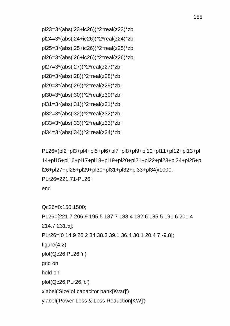
155
pl23=3*(abs(i23+ic26))^2*real(z23)*zb;
pl24=3*(abs(i24+ic26))^2*real(z24)*zb;
pl25=3*(abs(i25+ic26))^2*real(z25)*zb;
pl26=3*(abs(i26+ic26))^2*real(z26)*zb;
pl27=3*(abs(i27))^2*real(z27)*zb;
pl28=3*(abs(i28))^2*real(z28)*zb;
pl29=3*(abs(i29))^2*real(z29)*zb;
pl30=3*(abs(i30))^2*real(z30)*zb;
pl31=3*(abs(i31))^2*real(z31)*zb;
pl32=3*(abs(i32))^2*real(z32)*zb;
pl33=3*(abs(i33))^2*real(z33)*zb;
pl34=3*(abs(i34))^2*real(z34)*zb;
PL26=(pl2+pl3+pl4+pl5+pl6+pl7+pl8+pl9+pl10+pl11+pl12+pl13+pl
14+pl15+pl16+pl17+pl18+pl19+pl20+pl21+pl22+pl23+pl24+pl25+p
l26+pl27+pl28+pl29+pl30+pl31+pl32+pl33+pl34)/1000;
PLr26=221.71-PL26;
end
Qc26=0:150:1500;
PL26=[221.7 206.9 195.5 187.7 183.4 182.6 185.5 191.6 201.4
214.7 231.5];
PLr26=[0 14.9 26.2 34 38.3 39.1 36.4 30.1 20.4 7 -9.8];
figure(4.2)
plot(Qc26,PL26,'r')
grid on
hold on
plot(Qc26,PLr26,'b')
xlabel('Size of capacitor bank[Kvar]')
ylabel('Power Loss & Loss Reduction[KW]')

156
O. % Power factor & savings calculations for Capacitor on node 26
al = acos (0.85);
P = 3680;
A = 250;
C = 70;
Qc26 = 0:150:1500;
x = tan (al) – (Qc26/P);
a2 = atan (x);
y = cos (a2);
S26 = A.*((P./(cos(al))) – (P./(cos(a2))))-C.*(P.*tan(al)-P.*tan(al)-
P.*tan(a2))
Figure (1)
plot (Qc26, S26, ‘b’)
grid on
xlabel (‘Size of capacitor bank on node 26 [Kvar]‘)
ylabel (‘Savings [N]’)
P. % Power Factor & Savings Calculations for Capacitor on node 11
a1=acos(0.85);
P=1380;
A=250;
C=70;
for Qc=0:150:1500;
x=tan(a1)-(Qc/P);
a2=atan(x);
y=cos(a2);
S=A*((P/(cos(a1)))-(P/cos(a2))))-C*(P*tan(a1)-P*tan(a2));
end
Q. % Losses and Loss Reduction after addition of capacitor on node 11

157
for Qc11-0:150*1000:1500*1000;
ic26=(Qc26/V26)*i;
ic11=(Qc11/V11)*i;
p12=3*(abs(i2+ic11))^2*real(z2)*zb;
p13=3*(abs(i3+ic11))^2*real(z3)*zb;
p14=3*(abs(i4+ic11))^2*real(z4)*zb;
p15=3*(abs(i5+ic11))^2*real(z5)*zb;
p16=3*(abs(i6+ic11))^2*real(z6)*zb;
p17=3*(abs(i7+ic11))^2*real(z7)*zb;
p18=3*(abs(i8+ic11))^2*real(z8)*zb;
p19=3*(abs(i9+ic11))^2*real(z9)*zb;
p10=3*(abs(i10+ic11))^2*real(z10)*zb;
p111=3*(abs(i11+ic11))^2*real(z11)*zb;
p112=3*(abs(i12))^2*real(z12)*zb;
p113=3*(abs(i13))^2*real(z13)*zb;
p114=3*(abs(i14))^2*real(z14)*zb;
p115=3*(abs(i15))^2*real(z15)*zb;
p116=3*(abs(i16))^2*real(z16)*zb;
p117=3*(abs(i17))^2*real(z17)*zb;
p118=3*(abs(i18))^2*real(z18)*zb;
p119=3*(abs(i19))^2*real(z19)*zb;
p120=3*(abs(i20))^2*real(z20)*zb;
p121=3*(abs(i21))^2*real(z21)*zb;
p122=3*(abs(i22))^2*real(z22)*zb;
p123=3*(abs(i23))^2*real(z23)*zb;
p124=3*(abs(i24))^2*real(z24)*zb;
p125=3*(abs(i25))^2*real(z25)*zb;
p126=3*(abs(i26))^2*real(z26)*zb;
p127=3*(abs(i27))^2*real(z27)*zb;
p128=3*(abs(i28))^2*real(z28)*zb;

158
p129=3*(abs(i29))^2*real(z29)*zb;
p130=3*(abs(i30))^2*real(z30)*zb;
p131=3*(abs(i31))^2*real(z31)*zb;
p132=3*(abs(i32))^2*real(z32)*zb;
p133=3*(abs(i33))^2*real(z33)*zb;
p134=3*(abs(i34))^2*real(z34)*zb;
p=(p12+p13+p14+p15+p16+p17+p18+p19+p110+p111+p112+p11
3+p114+p114+p115
+p116+p117+p118+p119+p120+p121+p122+p123+p124+p125+p
126+p127+p128+p129
+p130+p131+p132+p133+p134)/1000
dI=221.71-p
end
R. % Power Factor and Savings calculations for Capacitor on node 11
al = acos (0.85);
P = 1380;
A = 250;
C = 70;
Qcll = 0:150:1500;
x = tan (al) – (Qc11/P);
a2 = atan (x);
y = cos (a2);
S11=(A.*((P./(cos(al)))- (P./(cos(a2))))-C.*(P.*tan(al) – P.*tan(a2)))
Figure (1)
plot (Qc11, S11, ‘b’)
grid on
xlabel (‘Size of capacitor bank on node 11 [Kvar]’)

159
ylabel (‘Savings [N]’)
S. % Power loss and loss reduction after placement of capacitor on
node 11(capacitors on nodes 26 & 11)
for Qc11=750*1000:150*1000:2250*1000;
ic11=(Qc11/V11)*ib;
pl2=3*(abs(i2+ic26+ic11))^2*real(z2)*zb;
pl3=3*(abs(i3+ic26+ic11))^2*real(z3)*zb;
pl4=3*(abs(i4+ic26+ic11))^2*real(z4)*zb;
pl5=3*(abs(i5+ic26+ic11))^2*real(z5)*zb;
pl6=3*(abs(i6+ic26+ic11))^2*real(z6)*zb;
pl7=3*(abs(i7+ic11))^2*real(z7)*zb;
pl8=3*(abs(i8+ic11))^2*real(z8)*zb;
pl9=3*(abs(i9+ic11))^2*real(z9)*zb;
pl10=3*(abs(i10+ic11))^2*real(z10)*zb;
pl11=3*(abs(i11+ic11))^2*real(z11)*zb;
pl12=3*(abs(i12))^2*real(z12)*zb;
pl13=3*(abs(i13))^2*real(z13)*zb;
pl14=3*(abs(i14))^2*real(z14)*zb;
pl15=3*(abs(i15))^2*real(z15)*zb;
pl16=3*(abs(i16))^2*real(z16)*zb;
pl17=3*(abs(i17+ic26))^2*real(z17)*zb;
pl18=3*(abs(i18+ic26))^2*real(z18)*zb;
pl19=3*(abs(i19+ic26))^2*real(z19)*zb;
pl20=3*(abs(i20+ic26))^2*real(z20)*zb;
pl21=3*(abs(i21+ic26))^2*real(z21)*zb;
pl22=3*(abs(i22+ic26))^2*real(z22)*zb;
pl23=3*(abs(i23+ic26))^2*real(z23)*zb;
pl24=3*(abs(i24+ic26))^2*real(z24)*zb;
pl25=3*(abs(i25+ic26))^2*real(z25)*zb;

160
pl26=3*(abs(i26+ic26))^2*real(z26)*zb;
pl27=3*(abs(i27))^2*real(z27)*zb;
pl28=3*(abs(i28))^2*real(z28)*zb;
pl29=3*(abs(i29))^2*real(z29)*zb;
pl30=3*(abs(i30))^2*real(z30)*zb;
pl31=3*(abs(i31))^2*real(z31)*zb;
pl32=3*(abs(i32))^2*real(z32)*zb;
pl33=3*(abs(i33))^2*real(z33)*zb;
pl34=3*(abs(i34))^2*real(z34)*zb;
PL2611=(pl2+pl3+pl4+pl5+pl6+pl7+pl8+pl9+pl10+pl11+pl12+pl13+
pl14+pl15+pl16+pl17+pl18+pl19+pl20+pl21+pl22+pl23+pl24+pl25
+pl26+pl27+pl28+pl29+pl30+pl31+pl32+pl33+pl34)/1000;
PLr2611=221.71-PL2611;
end
Qc2611=750:150:2250;
PL2611=[182.6 176.9 173.5 172.3 173.4 176.8 182.4 190.2 200.3 212.7
227.4];
PLr2611=[39.1 44.8 48.2 49.4 48.3 44.9 39.3 31.5 21.4 9 -5.7];
figure(4.3)
plot(Qc2611,PL2611,'r')
grid on
hold on
plot(Qc2611,PLr2611,'b')
xlabel('Size of capacitor bank[Kvar]')
ylabel('Power Loss & Loss Reduction[KW]')

161 T. % Power factor & Net Savings after Compensation
a1=acos(0.85);
P=3680;
A=250;
C=70;
for Qc2611=750:150:2250;
x=tan(a1)-(Qc/P);
a2=atan(x);
y=cos(a2);
S2611=A*((P/(cos(a1)))-(P/(cos(a2))))-C*(P*tan(a1)-P*tan(a2));
end
Qc2611=750:150:2250;
S2611=[33.4 36.7 38.8 39.5 38.9 36.9 33.4 28.5 22.1 14.2 4.8];
figure(4.4)
plot(Qc2611,S2611,'r')
grid on
xlabel('Size of capacitor bank[Kvar]')
ylabel('Net savings per annum[N]x10^3')
End