high precision refractive index measurement techniques
TRANSCRIPT

University of New MexicoUNM Digital Repository
Nuclear Engineering ETDs Engineering ETDs
Summer 7-1-2017
High Precision Refractive Index MeasurementTechniques Applied to the Analysis of NeutronDamage and Effects in CaF2 CrystalsJoseph P. Morris Ph.D.University of New Mexico
Follow this and additional works at: https://digitalrepository.unm.edu/ne_etds
Part of the Nuclear Engineering Commons, and the Optics Commons
This Dissertation is brought to you for free and open access by the Engineering ETDs at UNM Digital Repository. It has been accepted for inclusion inNuclear Engineering ETDs by an authorized administrator of UNM Digital Repository. For more information, please contact [email protected].
Recommended CitationMorris, Joseph P. Ph.D.. "High Precision Refractive Index Measurement Techniques Applied to the Analysis of Neutron Damage andEffects in CaF2 Crystals." (2017). https://digitalrepository.unm.edu/ne_etds/63

i
Joseph Paul Morris Candidate
Nuclear Engineering
Department
This dissertation is approved, and it is acceptable in quality and form for publication:
Approved by the Dissertation Committee:
Adam Hecht, Ph.D., Chairperson
Gary Cooper, Ph.D.
Cassiano de Oliveira, Ph.D.
Jean-Claude Diels, Ph.D.
ii
HIGH PRECISION REFRACTIVE INDEX MEASUREMENT
TECHNIQUES APPLIED TO THE ANALYSIS OF
NEUTRON DAMAGE AND EFFECTS IN CAF2 CRYSTALS
by
JOSEPH PAUL MORRIS
B.S. Electrical Engineering, Ohio University, 2010
M.S. Optoelectronic Engineering, Ohio University, 2012
DISSERTATION
Submitted in Partial Fulfillment of the
Requirements for the Degree of
Doctor of Philosophy
Engineering
The University of New Mexico
Albuquerque, New Mexico
July, 2017

iii
DEDICATION
To the Lord over all the Earth, and Savior of Mankind, Christ Jesus
“And whatsoever ye do, do it heartily, as to the Lord, and not unto men; Knowing that of
the Lord ye shall receive the reward of the inheritance: for ye serve the Lord Christ.”
Colossians 3:23-24
“Jesus saith unto him, I am the way, the truth and the
life: no man cometh unto the Father, but by me.”
John 14:6
“That if thou shalt confess with thy mouth the Lord Jesus, and shalt believe in
thine heart that God hath raised him from the dead, thou shalt be saved.”
Romans 10:9

iv
ACKNOWLEDGEMENTS
Above all I am most grateful to the Lord and Savior of the world Christ Jesus for
the sacrifice He made to give all life purpose and meaning. Without that sacrifice all the
work I have completed here would be a vain attempt on my part to give myself meaning
and purpose. He has blessed my family beyond measure during my time at the University
of New Mexico. He has taught me, most importantly, to emulate and display the love and
passion He has for all the people on Earth. I will continue to move forward offering my
work and all that I am as a living sacrifice to Him, for He is worthy of all that I can give.
I bestow thanks upon Dr. Adam Hecht, who has served as my graduate advisor. He
has provided valuable direction and resources necessary to completing this work. He has
also provided many challenges along the way that I am grateful for. Additionally, I would
like to thank the other members of my dissertation committee, Dr. Gary Cooper, Dr.
Cassiano de Oliveira, and Dr. Jean-Claude Diels. Their technical knowledge and expertise
has aided me in many ways during the pursuit of my doctorate degree.
I acknowledge the support of the Department of Energy, Nuclear Universities
Consortium, and the INL-LDRD, Award Number: 0145662 Release No. 007.
Additionally, I am grateful to the Department of Defense SMART scholarship program for
educational funding and the Air Force Nuclear Weapons Center for supporting this pursuit.
I would also like to acknowledge collaborative support of Maria Okuniewski, Sebastien
Teysseyre of Idaho National Laboratory, and the Center for Advance Computing Research
at the University of New Mexico.

v
I grant special recognition to James Hendrie. James was the cornerstone of the laser
physics aspect of this work and is deserving of great thanks. Additionally, Sara Pelka was
a crucial member of the research team and her assistance was greatly valued. I also bestow
thanks upon Major Jon Rowland, a true friend, who provided encouragement, expertise,
and prayer on my behalf.
I am deeply grateful for mother, Katherine Morris, late father, Dennis Morris. I am
thankful to my sisters, brothers-in-law, and sister-in-law, Jeff and Bethany Buckner, Randy
and April Massie, Michael and Linda Lacey, and Jessica Heim, as well as my father and
mother-in-law, Walter and Beverly Heim. I am also grateful to my friends Tucker and
Brittnee Barlow, grandparents-in-law Tom and Jeannie Heim, and many other family and
friends for their continued support and prayer.
I would especially like to thank my beautiful wife and wonderful children, Rachel
Morris, James, Isaiah, and John, for their continual love, support, and inspiration
throughout all the areas of my life. Rachel was beyond gracious and self-sacrificing in my
pursuit of this degree. She was extremely helpful in diagnosing some inconsistencies and
difficulties in my work while inspiring me to emulate Christ more and more.

vi
HIGH PRECISION REFRACTIVE INDEX MEASUREMENT
TECHNIQUES APPLIED TO THE ANALYSIS OF
NEUTRON DAMAGE IN CAF2 CRYSTALS
by
Joseph Paul Morris
B.S. Electrical Engineering, Ohio University, 2010
M.S. Optoelectronic Engineering, Ohio University, 2012
Ph.D. Engineering, University of New Mexico, 2017
ABSTRACT
Neutron irradiation damages material by atomic displacements. The majority of
these damage regions are microscopic and difficult to study, though they can cause a
change in density and thus a change in refractive index in transparent materials. This work
utilized CaF2 crystals to track refractive index change based on neutron radiation dose.
High precision refractive index measurements were performed utilizing a nested-cavity
mode-locked laser where the CaF2 crystal acted as a Fabry-Pérot Etalon (FPE). By
comparing the repetition rate of the cavity and the repetition rate of the FPE, refractive
index change was determined. Following several irradiation experiments, the change in
refractive index was measured to examine correlation between dose and the change in
refractive index.
An examination of the causal effects behind refractive index change was also
performed by molecular dynamics simulations, leading to a statistical determination of the
threshold displacement energy (TDE) in a CaF2 crystal lattice. Additionally, damage
cascade analysis suggests that the number of atomic displacements and vacancies caused
by neutron irradiation increases linearly as a function of incident neutron energy.

vii
Simulations were performed for a Primary Knock-on Atom (PKA) energy range of 100 eV
to 5 keV, which was the upper limit of the computing constraints for this work. This
finding is in line with the irradiation induced refractive index change theory for crystalline
solids.
Light irradiation of crystalline solids was performed demonstrating noticeable trends
in the change of refractive index when correlated to absorbed dose. Unfortunately, due to
uncertainties in the data caused by several unknown factors, higher dose irradiations must
be performed to confirm the trend. This type of experimental measurement of microscopic
damage in the bulk of the material through the refractive index will supports several
potential applications. This technique may be adopted and modified for dosimetry
applications as well as being utilized as a nondestructive method for understanding
microscopic neutron damage in bulk materials.

viii
Table of Contents
ABSTRACT ..................................................................................................................... VI
TABLE OF CONTENTS ............................................................................................ VIII
LIST OF FIGURES ......................................................................................................... X
LIST OF TABLES ..................................................................................................... XVII
CHAPTER 1: INTRODUCTION .................................................................................... 1
1.1 MOTIVATION .................................................................................................................................. 1 1.2 OVERVIEW ...................................................................................................................................... 1 1.3 PROBLEM DESCRIPTION .................................................................................................................. 5 1.4 SCOPE OF THIS DISSERTATION ........................................................................................................ 6
CHAPTER 2: NEUTRON RADIATION DAMAGE MODELING AND
SIMULATION .................................................................................................................. 8
2.1 OVERVIEW ...................................................................................................................................... 8 2.2 RADIATION DAMAGE & RECOVERY BACKGROUND ........................................................................ 9
2.2.1 Radiation Damage vs. Radiation Effects ................................................................................... 9 2.2.2 Types of Scattering and the PKA ............................................................................................. 11 2.2.3 Molecular Dynamics Models for Radiation Damage Analysis ................................................ 13 2.2.4 The Threshold Displacement Energy (TDE) ........................................................................... 16 2.2.5 The Damage Cascade .............................................................................................................. 17
2.3 LAMMPS MODELING SET UP ...................................................................................................... 22 2.3.1 Atomic Potential File Exploration ........................................................................................... 22 2.3.2 LAMMPS input file setup ......................................................................................................... 28 2.3.3 LAMMPS equilibration verification ........................................................................................ 30
2.4 LAMMPS DETERMINATION OF TDE ........................................................................................... 30 2.4.1 Methodology for Determining TDE ......................................................................................... 30 2.4.2 Calcium and Fluorine TDE Results ......................................................................................... 31 2.4.3 TDE Conclusions ..................................................................................................................... 33
2.5 LAMMPS DAMAGE CASCADE ..................................................................................................... 33 2.5.1 LAMMPS Damage Cascade Methodology .............................................................................. 33 2.5.2 PKA Energy Calculation ......................................................................................................... 34 2.5.3 Calcium PKA Cascade Results ................................................................................................ 35 2.5.4 Fluorine PKA Cascade Results ............................................................................................... 37 2.5.5 LAMMPS Cascade Modeling Conclusions .............................................................................. 39
2.6 MODELING AND SIMULATION CONCLUSIONS ............................................................................... 40
CHAPTER 3: MEASURING REFRACTIVE INDEX CHANGE OPTICALLY .... 42
3.1 OVERVIEW .................................................................................................................................... 42 3.2 OPTICAL METHODS FOR MEASURING RADIATION EFFECTS .......................................................... 42
3.2.1 Refractive Index Overview ....................................................................................................... 44 3.2.2 Mode-locked laser cavity ......................................................................................................... 47 3.2.3 The Fabry-Pérot Etalon........................................................................................................... 50 3.2.4 Generation of High Frequency Pulse Trains ........................................................................... 51
3.3 MEASURING THE CHANGE OF REFRACTIVE INDEX OPTICALLY .................................................... 57 3.3.1 Coupling Resonance Conditions of an FPE in a nested-cavity ............................................... 57 3.3.2 Mode-Locked Laser Cavity Pulse Width ................................................................................. 59 3.3.3 Nested-Cavity Pulse Bunches and Frequency Combs ............................................................. 62 3.3.4 Quantifying the Change in Refractive Index ............................................................................ 64 3.3.5 Angular and Cavity Length Dependence ................................................................................. 65 3.3.6 Finding the FPE Zero Angle ................................................................................................... 67

ix
3.3.7 Reproducing Cavity Length Range .......................................................................................... 69 3.4 EXPERIMENTAL SETUP ................................................................................................................. 70 3.5 LASER CAVITY CALIBRATION AND REPEATABILITY MEASUREMENTS ......................................... 71
3.5.1 Cavity Length Scans vs. Angle Scans ...................................................................................... 71 3.5.2 Finding the Zero Angle ............................................................................................................ 81 3.5.3 Crystal Rotation Experiment ................................................................................................... 83
3.6 CONTROL SAMPLES AND DAILY VARIATION ................................................................................ 90 3.7 CALIBRATION AND REPEATABILITY CONCLUSIONS ...................................................................... 92
CHAPTER 4: IRRADIATION METHODOLOGY .................................................... 93
4.1 CRYSTAL IRRADIATION METHODOLOGY ...................................................................................... 93 4.1.1 NH-3 Neutron Howitzer Irradiation ........................................................................................ 94 4.1.2 Sandia National Labs Irradiation ............................................................................................ 96 4.1.3 Oregon State University Irradiation ........................................................................................ 97
4.2 ESTIMATING RADIATION FLUENCE, ENERGY FLUENCE, AND DOSE WITH MCNP ......................... 97 4.2.1 NH-3 Neutron Howitzer MCNP Modeling .............................................................................. 98 4.2.2 Sandia National Labs Irradiation Dose Estimation .............................................................. 107 4.2.3 Oregon State University Irradiation Dose Estimation .......................................................... 108
CHAPTER 5: CAF2 IRRADIATION RESULTS AND ANALYSIS ....................... 110
5.1 OVERVIEW .................................................................................................................................. 110 5.2 OBTAINING RESULTS .................................................................................................................. 111 5.3 CORRECTING FOR DAILY VARIATION IN FREQUENCY RATIOS .................................................... 112 5.4 NH-3 NEUTRON HOWITZER IRRADIATION EXPERIMENTS ........................................................... 118 5.5 SANDIA NATIONAL LABORATORIES D-D AND D-T IRRADIATION EXPERIMENT ......................... 120 5.6 OSU TRIGA IRRADIATION EXPERIMENT ................................................................................... 125 5.7 COMBINING EXPERIMENT RESULTS ............................................................................................ 133 5.8 DATA TRENDS ............................................................................................................................ 134
CHAPTER 6: CONCLUSIONS .................................................................................. 140
6.1 NEUTRON DAMAGE AND EFFECTS MODELING ............................................................................ 140 6.2 CRYSTAL IRRADIATION AND REFRACTIVE INDEX TRACKING ..................................................... 141
CHAPTER 7: FUTURE WORK ................................................................................. 142
7.1 MESO-SCALE MODELING AND REFRACTIVE INDEX CHANGE PREDICTION ................................. 142 7.2 IRRADIATION EXPERIMENTATION ............................................................................................... 142 7.3 FIBER ANALYSIS ......................................................................................................................... 143 7.4 UNCERTAINTY AND ERROR ANALYSIS ....................................................................................... 143 7.5 ADDITIONAL IRRADIATION AND CRYSTAL VARIETY .................................................................. 144
REFERENCES .............................................................................................................. 145
APPENDIX A ................................................................................................................ 151
A.1 LAMMPS TDE EQUILIBRATION INPUT FILE .............................................................................. 151 A.2 LAMMPS TDE INPUT FILE (EXAMPLE) ..................................................................................... 154 A.3 LAMMPS CASCADE EQUILIBRATION INPUT FILE ...................................................................... 157 A.4 LAMMPS CASCADE 1000 KEV PKA INPUT FILE (EXAMPLE) .................................................... 161
APPENDIX B ................................................................................................................ 164
B.1 OVERVIEW .................................................................................................................................. 164 B.2 REPETITION RATE CHANGE WITH LABORATORY ENVIRONMENT CHANGES ............................... 164 B.3 FPE REPETITION RATE WITH LABORATORY ENVIRONMENT CHANGES ...................................... 167 B.4 FREQUENCY RATIO DELTA WITH LABORATORY ENVIRONMENT CHANGES ................................ 168 B.5 FREQUENCY RATIO WITH AIR DENSITY AND REFRACTIVE INDEX OF AIR ................................... 170
x
List of Figures
Figure 1.2.1: Results of Sand et al. [3] work showing that the vast majority of defects in a
material are too small to see visually. ................................................................................. 2
Figure 1.2.2: As higher energy particles enter a material they will naturally produce not
just a single PKA, but rather will generate many PKAs that will in turn interact with other
atoms within the lattice while the neutrons interact by collision with the nucleus ............. 3
Figure 2.2.1: Depiction of a classical elastic collision between two particles of different
mass................................................................................................................................... 12
Figure 2.2.2: Early theory depiction or radiation induced PKA displacement cascade [33].
........................................................................................................................................... 18
Figure 2.2.3: Later quantitative version of radiation induced PKA displacement spike
presented by Seeger [34]. .................................................................................................. 19
Figure 2.2.4: Radiation induced displacement cascade as simulated by Orlander displaying
the PKA path, secondary knock-on path, and higher order knock-ons [13]. .................... 20
Figure 2.2.5: Depiction of a sample damage cascade caused by a 10 keV gold (Au) atom
within a gold Face-Centered Cubic (FCC) lattice, similar to CaF2 [35]. .......................... 21
Figure 2.3.1: Plot of the fluorine-fluorine interaction potentials demonstrating the error in
the BMH potential for small atomic separations (the exponentially attractive force in the
negative direction), the error in the ZBL potential at large atomic separations (the excess
repulsive force), and the spline potential generated by atsim.potentials to create a more
correct overall potential. ................................................................................................... 26
Figure 2.3.2: Plot of the calcium-fluorine interaction potentials demonstrating the error in
the BMH potential for small atomic separations (not as repulsive as it should be at smaller
separations), the error in the ZBL potential at large atomic separations (not as attractive as
it should be at larger separations), and the spline potential generated by atsim.potentials to
create a more correct overall potential. ............................................................................. 27
Figure 2.4.1: Statistical determination of probability of displacement for a Ca atom within
a CaF2 crystal lattice. ........................................................................................................ 32
Figure 2.4.2: Statistical determination of probability of displacement for a Ca atom within
a CaF2 crystal lattice. ........................................................................................................ 32
Figure 2.5.1: Plot of lattice vacancies by Ca PKA with varying energies from 0 to 11
picoseconds. ...................................................................................................................... 36

xi
Figure 2.5.2: Plot and trendline for persistent damage at 11 picoseconds after initial self-
annealing events. Equation and R2 value define the trendline. ........................................ 37
Figure 2.5.3: Plot of lattice vacancies by F PKA with varying energies from 0 to 11
picoseconds. ...................................................................................................................... 38
Figure 2.5.4: Plot and trendline for persistent damage from F PKA at 11 ps after initial self-
annealing events. Equation and R2 value define the trendline. ........................................ 39
Figure 3.2.1: As higher energy particles enter a material they will naturally produce not
just a single PKA, but rather will generate many PKAs that will in turn interact with other
atoms within the lattice while the neutrons interact by collision with the nucleus ........... 43
Figure 3.2.2: f0 in this figure is the frequency domain representation of the round trip phase
slippage, Δφ. The mode spacing is representative of the cavity repetition rate, frep [8]. . 49
Figure 3.2.3: Demonstration of general function of a mode-locked laser cavity generating
singular pulses in the time domain at a rate determined by the cavity length. The pumping
laser enters from the left [8]. ............................................................................................. 51
Figure 3.2.4: Depiction of general function of a nested cavity mode-locked laser cavity
generating pulse bunches in the time domain at a rate determined by the cavity length. The
separation of the peaks within the bunch corresponds to the effective length of the FPE [8].
........................................................................................................................................... 52
Figure 3.2.5: Pulse Propagation in an FPE assuming pulse duration is much shorter than
the round trip time of the FPE [8]. .................................................................................... 53
Figure 3.2.6: The output of a nested-cavity mode-locked laser (bottom) as it is compared
to that of an identical cavity not containing an FPE (top) [8]. .......................................... 55
Figure 3.2.7: The RF spectrum of a single mode-locked laser (Top) containing no FPE.
The RF spectrum of a nested-cavity mode-locked laser (Bottom) with 15 mm fused silica
FPE. The repetition rate of both lasers were set to the same value. The inset plot (Middle)
demonstrates train shift resulting from the formation of pulse bunches [8]. .................... 56
Figure 3.2.8: Picture of a CaF2 FPE utilized in this research. This FPE is the 20.3 mm
diameter sample. ............................................................................................................... 57
Figure 3.3.1: Plot of an Interferometric Autocorrelation of the linear laser cavity without
an FPE operating at 7.01W and 790nm. ........................................................................... 60
Figure 3.3.2: Autocorrelation plot showing the multiple pulse train caused by the insertion
of the CaF2 FPE insterted at an internal angle of 8 mrad into a linear laser cavity operating
at 7.01W and 790nm. ........................................................................................................ 61
xii
Figure 3.3.3: Enhanced plot central pulse of an Interferometric Autocorrelation of the linear
laser cavity operating at 7.01W, 790nm, with a CaF2 FPE inserted at an internal angle of 8
mrad. ................................................................................................................................. 62
Figure 3.3.4: Time domain representation of two pulse bunches within the laser cavity
setup. The inset plot shows a close up of the first pulse bunch. ...................................... 63
Figure 3.3.5: Frequency domain representation of the pulse bunches within the laser cavity,
featuring well defined frequency combs whose central peaks correspond directly to the
repetition rate of the FPE. ................................................................................................. 63
Figure 3.3.6: A simplified depiction of a laser cavity emphasizing the constant cavity length
requirement for an angle scan to determine the refractive index change of an FPE. ....... 66
Figure 3.3.7: A simplified depiction of a laser cavity emphasizing the constant FPE angle
requirement for a cavity length scan to determine the refractive index change of an FPE.
........................................................................................................................................... 67
Figure 3.3.8: Demonstration of the position of the Photodetector (Det1) with respect to the
standard laser cavity comprised of two focusing mirrors (M1) and a Fabry-Pérot Etalon
(FP). .................................................................................................................................. 68
Figure 3.3.9: Generalized ideal depiction of the photodetector data as the internal angle of
the FPE is adjusted from a high positive internal angle to a high negative internal angle.
........................................................................................................................................... 69
Figure 3.4.1: A detailed rendering of the laser cavity setup for measuring refractive index
change in a material, where M1 is the focusing mirror, P1 and P2 are prisms, MQW is the
Multiple Quantum Well, F1 is the Focussing Lense, Det1 and Det2 are the Low Frequency
and High Frequency detectors, and FP is the Fabry-Pérot Etalon. ................................... 70
Figure 3.5.1: Frequency ratio data for each of four separate angle scan trial on March 8,
2016, each represented by a different color and associated dotted line representing the
standard deviations of each point in the trial. ................................................................... 73
Figure 3.5.2: Overall average frequency ratio data with overall standard deviation from
angle scans on March 8, 2016. .......................................................................................... 73
Figure 3.5.3: Close up of Figure 3.5.2 region of interest with statistical analysis boasting
standard deviation of 3.869x10⁻⁴....................................................................................... 74
Figure 3.5.4: Frequency ratio data for each of four separate angle scan trial on March 9,
2016 each represented by a different color and associated dotted line representing the
standard deviations of each point in the trial. ................................................................... 75

xiii
Figure 3.5.5: Overall average frequency ratio data with overall standard deviation from
angle scans on March 9, 2016. .......................................................................................... 75
Figure 3.5.6: Close up of Figure 3.5.5 region of interest with statistical analysis boasting a
standard deviation of 2.781x10⁻⁴....................................................................................... 76
Figure 3.5.7: Frequency ratio data from four separate trials on March 9, 2016 with an
overall cavity length change of 1 mm. .............................................................................. 78
Figure 3.5.8: Overall average frequency ratio data (all four trials) with overall standard
deviation from cavity length scans on March 9, 2016. Statistical analysis shows a standard
deviation of 3.066x10⁻⁵ ..................................................................................................... 78
Figure 3.5.9: Frequency ratio data from four separate trials on March 10, 2016 with an
overall cavity length change of 1 mm. .............................................................................. 79
Figure 3.5.10: Overall average frequency ratio data (all four trials) with overall standard
deviation from cavity length scans on March 10, 2016. Statistical analysis shows a standard
deviation of 6.443x10⁻⁶ ..................................................................................................... 79
Figure 3.5.11: Frequency ratio data from four separate trials on March 11, 2016 with an
overall cavity length change of 1 mm. .............................................................................. 80
Figure 3.5.12: Overall average frequency ratio data (all four trials) with overall standard
deviation from cavity length scans on March 11, 2016. Statistical analysis shows a standard
deviation of 2.397x10⁻⁶ ..................................................................................................... 80
Figure 3.5.13: Demonstration of the determination of the zero angle as measured for sample
A15-1. The local minimum in the center reveals the zero angle. The minimum point in
theory is the exact zero angle. ........................................................................................... 82
Figure 3.5.14: Plot depicting the LF/HF frequency ratio as a function of rotational angle
when rotated with a 2 RPM motor. ................................................................................... 84
Figure 3.5.15: Depiction of the rotational mount with descriptions of the pitch, yaw, and
roll directions used for these experiments. ....................................................................... 85
Figure 3.5.16: Plot demonstrating LF, HF, ratio, and zero angle data for the rotational
experiment with CaF2. ...................................................................................................... 86
Figure 3.5.17: Plot demonstrating LF, HF, ratio, and zero angle data for the rotational
experiment with SiO2. ....................................................................................................... 87
Figure 3.5.18: Simple depiction of the FPE mount, (a) demonstrates the perfect placement
of an FPE, (b) demonstrates the potential effect of tightening the set screw that can change
the zero angle. The crystal is oriented in this figure so the laser path is left and right. ... 88

xiv
Figure 3.5.19: Plot depicting the tilt setting to find the zero angle as a function of rotation
for a sample placed normally and the same sample placed intentionally at a dramatic tilt.
........................................................................................................................................... 89
Figure 3.6.1: Demonstration of the change in the frequency ratio for sample A15-1 over a
period of two weeks. The standard deviaiton of the entire population was 1.37x10⁻⁶ .... 90
Figure 3.6.2: Demonstration of the change in the frequency ratio for sample A15-2 over a
period of two weeks. The standard deviaiton of the entire population was 1.536x10⁻⁶ .. 91
Figure 4.1.1: Photo of the NH-3 Neutron Howitzer by Nuclear Chicago ........................ 95
Figure 4.1.2: Example schematic of experimental setup for generating D-T neutrons at
Sandia National Laboratory .............................................................................................. 97
Figure 4.2.1: Source Spectrum for in a PuBe source with varying Pu content [59]. ........ 99
Figure 4.2.2: XY-plane view of the MCNP geometries for the NH-3 Neutron Howizer with
15 mm CaF2 sample inserted (as region 9). .................................................................... 100
Figure 4.2.3: XZ-plane view of the MCNP geometries for the NH-3 Neutron Howizer with
15 mm CaF2 sample inserted (as region 9). .................................................................... 101
Figure 4.2.4: MCNP calculated flux distribution in CaF2 samples. ................................ 102
Figure 4.2.5: Estimated dose rate in CaF2 samples based on the number of days in the NH-
3....................................................................................................................................... 107
Figure 4.2.6: Plot of the MCNP and STAY’SL flux profile in the GRICIT-C region of the
OSU TRIGA reactor. All doses in this work were calculated using the MCNP flux values.
......................................................................................................................................... 109
Figure 5.3.1: Variation in frequency ratio of unirradiated control samples A15-1 and A15-
2, as well as the later included control samples B15-1 and B15-2. The total time period of
measurements occurred between June 29, 2016 and May 5, 2017. ................................ 113
Figure 5.3.2: Secondary daily variation experiment with much better laboratory
environment stability. ..................................................................................................... 114
Figure 5.3.3: Confidence error in measurement correction by measurement day to be
applied to the refractive index change calculated in the irradiated sample. ................... 117
Figure 5.4.1: Demonstration of the Change in Refractive Index in CaF2 sample A15-4
which was exposed to PuBe Source Neutron Irradiation in the NH-3 Neutron Howitzer for
221 days. ......................................................................................................................... 119

xv
Figure 5.4.2: Final Neutron Howitzer irradiation with sample A15-6 irradiated from 0 to 7
days. ................................................................................................................................ 120
Figure 5.5.1: Demonstration of the full data set for the Sandia irradiated sample (A15-5)
measured on eight separate occasions post irradiation and three separate pre-irradiation
measurements. ................................................................................................................. 121
Figure 5.5.2: Mean values for the baseline and irradiated measurents for the Initial Sandia
irraidated sample having recieved 3.15 Gy in absorbed dose. ........................................ 122
Figure 5.5.3: Initial Sandia irradiation results including overall uncertainty. ................ 124
Figure 5.5.4: Refractive index change results for Sandia irradiations of sample A15-5. 125
Figure 5.6.1: Side-by-side comparison of the OSU irradiated sample B15-5 and the non-
irradiated control sample B15-1. This photograph demonstrates a darkening in the crystal
due to the harsh environment of the OSU TRIGA reactor. ............................................ 126
Figure 5.6.2: Demonstration of the "bleaching" effect that occurred after attemping to
mode-lock the cavity with this FPE inserted. ................................................................. 127
Figure 5.6.3: Sample B15-5 after approximately 2 hours exposure to high intensity green
light effectively "bleaching" out color center in the CaF2 sample. ................................. 128
Figure 5.6.4: Sample B15-5 after 36 hours exposure to high intensity UV light, resulting in
a transmission value at 792 nm of 84.72%. .................................................................... 129
Figure 5.6.5: Sample B15-5 after a total of 96 hours of exposure to high intensity UV light,
resulting, in an transmission value at 792 nm of 89.33%. .............................................. 130
Figure 5.6.6: Image of unirradiated and irradiated CaF2 crystals. Unirradiated on left and
irradiated organized from left to right with least to most irradiation. ............................. 131
Figure 5.6.7: Refractive index change measurement results from OSU irradiated samples.
B15-4 was irradiated to 1.99x10⁴ Gy. B15-5 was irradiated to 1.99x10⁵ Gy. B15-3 was
irradiated to 1.99x10⁶ Gy. ............................................................................................... 132
Figure 5.7.1: Refractive index change measured in all irradiated CaF2 samples as a function
of absorbed dose. ............................................................................................................ 134
Figure 5.8.1: Recreation of Primak [5] refractive index measurement data. .................. 135
Figure 5.8.2: Plot of irradiation data on a linear scale demonstrating a decreasing trend in
refractive index on average. The dotted line represents a linear curve fit of the data. .. 137
Figure 5.8.3: Plot of all irradiation data on a semi-log scale. ......................................... 137

xvi
Figure B.1: Cavity repetition rate and relative humidity as measured on days the NH-3
Howitzer sample (A15-4) was measured for refractive index change. ........................... 165
Figure B.2: Cavity repetition rate and relative humidity as measured on days the NH-3
Howitzer sample (A15-4) was measured for refractive index change ............................ 166
Figure B.3: FPE repetition rate and relative humidity as measured on days the NH-3
Howitzer sample (A15-4) was measured for refractive index change. ........................... 167
Figure B.4: FPE repetition rate and pressure as measured on days the NH-3 Howitzer
sample (A15-4) was measured for refractive index change. ........................................... 168
Figure B.5: Frequency ratio and relative humidity as measured on days the NH-3 Howitzer
sample (A15-4) was measured for refractive index change. ........................................... 169
Figure B.6: Frequency ratio and pressure as measured on days the NH-3 Howitzer sample
(A15-4) was measured for refractive index change. ....................................................... 169
Figure B.7: Frequency ratio and air density as measured on days the NH-3 Howitzer sample
(A15-4) was measured for refractive index change. ....................................................... 171
Figure B.8: Frequency ratio and refractive index of air as measured on days the NH-3
Howitzer sample (A15-4) was measured for refractive index change. ........................... 171

xvii
List of Tables
Table 2.3.1: Published pair wise potential style parameters for BMH, Buckingham, and
Modified Buckingham styles for interactions within CaF2............................................... 24
Table 2.5.1: A table showing the velocity of a PKA in Angstroms/Picosecond based on the
desired PKA energy. ......................................................................................................... 35
Table 4.1.1: Table showing the physical measurements of the first set of CaF2 samples. 94
Table 4.1.2: Table showing the physical measurements of the second set of CaF2 samples.
........................................................................................................................................... 94
Table 4.2.1: Values of Dose Factor and Quality Factor for converting flux-to-dose per
NCRP-38 and ANSI/ANS-6.1.1-1977. ........................................................................... 104
Table 4.2.2: Comparison of Dose values calculated by kerma factor and by dose factor
using a discretized sampling of the flux spectrum as generated by the MCNP code. .... 105
Table 4.2.3: Kerma Factors for CaF2 as quoted from Caswell [62]. .............................. 106
Table 5.1.1: Master table showing the neutron fluence, energy fluence and absorbed dose
values associated with each irradiated CaF2 sample. Doses were calculated using MCNP
and provided fluence values for energies above 2 keV. Per Chapter 2, 2 keV is close to the
required neutron energy to create a PKA that will cause a damage cascade. ................. 110

1
Chapter 1: Introduction
1.1 Motivation
Neutron irradiation can cause atomic displacements (damage) in a material, which in
turn, can cause swelling or compaction. This effect does not occur for gamma irradiation
at typical reactor energies. This swelling or compaction causes a change in density, which
manifests itself in transparent materials as a change in refractive index and can be
measured. The great majority of the damage from neutron irradiation occurs in
microscopic displacements, and these displacements account for the majority of the large-
scale radiation effects. These displacements are difficult to measure through traditional
methods [1], and are especially difficult to measure nondestructively in the bulk of the
material. The primary goal of this work is to apply techniques for very high precision
refractive index measurements to crystals that have been irradiated, towards using this
technique as a mode of understanding radiation damage and dose through the material.
This allows for a nondestructive assessment of radiation effects in a material that may be
used to improve damage models. This may also open the door for a family of new materials
for radiation detection, measurement, and dosimetry. Ultimately the hope of this effort is
to demonstrate a novel technology that will enable high precision dosimetry in real time
harsh radiation environments.
1.2 Overview
The work described in this dissertation is focused on material damage, effects, and
refractive index change due to neutron irradiation of Calcium Fluoride, CaF2. This work
was completed utilizing modeling, simulation, and experimental analysis. The focus of the

2
modeling and simulation aspects is the cultivation of an understanding of damage
propagation within CaF2. By extracting the Threshold Displacement Energy (TDE) of Ca
and F atoms and modeling the damage cascades this work will inform future analysis
linking large-scale property changes such as refractive index and density to these small-
scale damage cascades. This is extremely important as most radiation induced effects of
material properties are caused by microscopic defects [1], and defects below 5 nm are
responsible for most the changes in material properties [2]. This is further exhibited by
Sand et al. where it is shown that the frequency of defects generated per ion follows a
power law in which the vast majority of defects impacting the material are microscopic
and too small to detect visually [3] [4], as shown in Figure 1.2.1.
Figure 1.2.1: Results of Sand et al. [3] work showing that the vast majority
of defects in a material are too small to see visually.
3
The vast majority of defect populations under irradiation are very small and cannot
be detected visually. This is precisely where the methods presented in this work are useful.
This optical technique can examine the sum result of these microscopic effects in the
material, which enhances the potential applications of this technique.
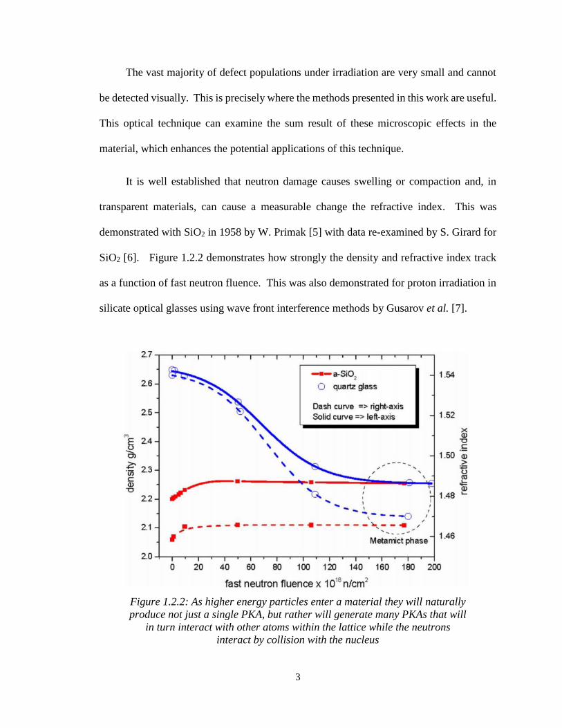
It is well established that neutron damage causes swelling or compaction and, in
transparent materials, can cause a measurable change the refractive index. This was
demonstrated with SiO2 in 1958 by W. Primak [5] with data re-examined by S. Girard for
SiO2 [6]. Figure 1.2.2 demonstrates how strongly the density and refractive index track
as a function of fast neutron fluence. This was also demonstrated for proton irradiation in
silicate optical glasses using wave front interference methods by Gusarov et al. [7].
Figure 1.2.2: As higher energy particles enter a material they will naturally
produce not just a single PKA, but rather will generate many PKAs that will
in turn interact with other atoms within the lattice while the neutrons
interact by collision with the nucleus

4
The purpose of the current research is to demonstrate that that the change of
refractive index can be tracked in a crystal with the high precision technique developed by
J.-C. Diels at the University of New Mexico [8]. A brief proof of concept for CaF2 showed
that this technique provides very high precision measurements of the change of refractive
index [9]. The utilization of this optical technique is of paramount importance to this work
and is described in detail in Chapter 3.
The work in this dissertation has been successful in measuring refractive index
change following neutron irradiation. To set the stage for future applications, this could
serve for active reading of crystals undergoing neutron damage by optically coupling the
crystals to the optical analysis setup to be described, such as with optical fiber. In fact,
Cheymol et al., 2008, studied the effect of high level gamma and neutron irradiation on
silica optical fibers [10]. Through the utilization of the CEA OSIRIS Nuclear Reactor they
attained a fast neutron fluence of 1.3x10²⁰ n/cm2 with a dose of 16 GGy. While that work
did not address refractive index, they examined the effects of radiation on transmission
spectra in fibers, which is the difficulty with using optical fibers in radiation environments.
They showed absorption minima in the near infrared (IR) and the IR region utilizing
particularly high purity silica and hollow core photonic bandgap fibers. This is the
wavelength range in which the optical technique demonstrated here operates, opening the
future possibility of using it with fiber optics in a high radiation environment.
It should be noted that there are three primary types of instruments used to measure
radiation fields: detectors, which give an active response; monitors, which often produce a
vague response such as crossing a threshold; and dosimeters, which are usually integrating
in nature and are used for a later read out. This research focuses on utilizing CaF2 as an

5
integrating dosimeter. By coupling the readout to the crystal while it is in the radiation
field, such as with fiber optics, it will be possible for the crystal then to be used as a detector
with a live-time readout.
1.3 Problem Description
Neutron irradiation damages materials by producing lattice dislocations, which
create voids and in general causes swelling in a material, decreasing the material density.
In some materials, there may be compaction and thus an increase of density. In either case
the analysis contained herein would still apply. Swelling is correlated with a decrease in
the index of refraction, which can be measured with high precision. In June 2015, our group
measured the frequency ratio (described in more detail in Chapter 3), used in our technique
to extract the refractive index, with a standard deviation of the mean of 3x10⁻⁸ [9]. With a
goal as hopeful as enabling high precision neutron dosimetry, and moving towards high-
precision real-time neutron dosimetry there are many challenges along the way. Here they
will be presented beginning with radiation damage and concluding with crystal based
dosimetry. Challenges that have been encountered, or are expected to be encountered,
follow.
Modeling, simulation, and experiments were performed to understand radiation
damage in CaF2. For simulations, there is a significant lack of radiation damage molecular
dynamics (MD) research on CaF2. This requires a combination of potential energy files to
analyze collisions at small atomic separations. Moving from the MD atomic lattice scale
to the meso-scale also presented challenges as many of the meso-scale models do not take
into account crystal structure and there is expected to be some error in the modeling.

6
The measurement of the dose in the crystals by subsequently measuring the refractive
index utilizing a nested Fabry-Pérot Etalon (FPE) in linear laser cavity was the most
challenging aspect to this research as inevitably, high precision results depend very heavily
on high precision instruments and are thus very sensitive to uncertainties. These are
detailed later in this work. The characterization and repeatability analysis of this method
is essential for moving forward. The estimation of received dose in the crystal samples
also presented a challenge. Although with the aid of MCNP, published neutron kerma
factors, and accurate modeling of the radiation field, the estimation of dose is at the very
least, consistent throughout the research.
The final challenge in the current work was irradiating CaF2 samples neutrons and
observing refractive index changes. This has been done over a range of neutron energy
fluences and doses to examine trends in the refractive index.
1.4 Scope of this Dissertation
There were several primary goals of this research, in both calculation and
experimentation. The first was to understand the collision physics within crystalline
materials on the atomic scale. This was accomplished by determining the Threshold
Displacement Energy (TDE) of both calcium (Ca) and fluorine (F) atoms in a CaF2, face
centered cubic (FCC) crystal structure and performing small-scale damage cascade
analysis. This utilized LAMMPS Molecular Dynamics (MD) code and is discussed in
thorough detail in Chapter 2. The second goal, which is the major goal of this work, was
measuring the refractive index change from neutron irradiation of a sample. Doing this
required a thorough characterization of the nested-cavity method of determining refractive
7
index change. This is discussed in Chapter 3. Next, the design of the experimental
irradiation method and dose calculation standard is presented in Chapter 4. The resulting
effects of the neutron irradiation are discussed in Chapter 5 along with the correlation of
the crystal damage, dose, and refractive index change. This is followed by the overall
conclusions in Chapter 6. A brief discussion of the future steps to expand this research is
contained in Chapter 7.

8
Chapter 2: Neutron Radiation Damage Modeling and Simulation
2.1 Overview
Understanding the propagation of radiation damage in a material is paramount to
predicting the material damage effects. It has been assumed that the Displacements per
Atom (DPA) value is the most accurate way to determine what will happen to a material
in the large scale when considering a small-scale calculation. However, it has been shown
more recently that the correlation between DPA and material effects is in many cases
secondary or coincidental [1]. In fact, the expectation and demonstration from Dethloff
[1] is that small defects, in a region of 5 nm or less, are responsible for the majority of the
changes in material properties. Given this fact, it was necessary at the beginning of this
work to study the propagation of damage and small scale defects in CaF2. This can be
approached with molecular dynamic (MD) simulations.
The modeling and simulation in this work is comprised of two primary components,
both of which are detailed in this chapter. First, the method for determining the baseline
properties of damage, namely, the TDE of Calcium and Fluorine atoms in CaF2 is
discussed. Second, the method for utilizing LAMMPS (Large-scale Atomic/Molecular
Massively Parallel Simulator) [11] for basic damage cascade simulations, atom recoil
energies up to 5 keV, and the extrapolation of that data to higher energies, is presented.
All simulations were performed utilizing the Center for Advanced Research Computing
(CARC) at the University of New in Albuquerque, NM. A major consideration of the
damage cascade analysis is the expectation of what is termed self-annealing. This is a well-
understood property of a crystalline material that allows for re-crystallization after a
9
damage cascade occurs [12], and is examined in the short time scales of the MD
simulations. Crystalline materials have been shown to hold up to the intense environments
of radiation fields better that most materials specifically because of this self-annealing
effect.
2.2 Radiation Damage & Recovery Background
2.2.1 Radiation Damage vs. Radiation Effects
The specific terminology used in describing irradiated materials is important to
define. "Radiation damage" generally refers to atomic displacement, or the microscopic
events that produce the appearance of large-scale changes in a solid [13]. In other words,
damage occurs when there are individual interactions inside a material. For incident
neutrons, this is primarily through nuclear scattering collisions. This may cause atomic
displacements producing lattice vacancies and, where the displaced atom stops,
interstitials. The field of radiation damage has benefited greatly from high power computer
processing as much of this field relies on computer simulation of lattices to understand the
damage cascades that take place on an atomic level when an incident particle collides and
directly knocks an atom out of its lattice position. This displaced atom that recoils directly
from the incident particle is referred to as a Primary Knock-on Atom (PKA), and there can
be many PKAs from a single incident particle, but this distinguishes them from the cascade
that often follows. There are several robust programs today that can be used to build lattice
structures and simulate damage cascades. The primary program utilized in this research is
called LAMMPS and was developed by Sandia National Laboratories.

10
"Radiation effects" on the other hand generally refers to the “macroscopic,
observable, and often technologically crucial results of exposure of solids to energetic
particles” [13]. Unlike radiation damage, radiation effects can be studied without the aid
of computer simulations, though experimental research in this area is typically supported
and substantiated by meso-scale simulations. These meso-scale simulations are beyond
the scope of the current, primarily experimental, work.
The ultimate goal of each is to predict the large-scale effects of radiation on a material
and specifically determine how its intrinsic properties will be changed as a result of
irradiation. In many cases these models are aided by prior molecular dynamics simulation
to determine baseline radiation damage properties of the material such as, in particular, the
Threshold Displacement Energy of each of the types of atoms in the material.
The primary concern exploring radiation damage is in predicting the configuration
and total number of vacancies and interstitial sites within a material based on the
characteristics of the material and the bombarding particles. The field of radiation effects
is primarily concerned with the bulk effects of radiation damage on large scale material
properties, the macroscopic or large scale results of radiation exposure.
As mentioned, the terms "radiation damage" and "radiation effects" are frequently
interchanged as if they mean the same thing but it is important in this research to distinguish
between them early on. One key distinguishing factor between the two is time scale.
Radiation damage takes place within 10s of picoseconds of a particle collision. The
subsequent radiation effect processes that change material properties take much longer.
That timing ranges widely and can be milliseconds for some diffusion processes, while in
metals some processes take months to form noticeable effects [13]. This is important for

11
the consideration of the long-term recovery of a material, which is one of the things that is
explored in this research. The bulk of the modeling and simulation of this research is
concerned with radiation damage and ultimately how damage propagates in single PKA
systems. By focusing on this aspect several key factors can be extracted that can then
inform the amount and type of defects that may form in a larger scale irradiation.
2.2.2 Types of Scattering and the PKA
In radiation damage the incident particle collides with an atomic nucleus in a lattice
structure, the PKA. The energy transferred to the PKA varies greatly depending on the
energy of the incident particle and the angle of the collision.
There are three primary types of neutron interactions: capture, elastic scatter, and
inelastic scatter. In capture, when a neutron collides with a nucleus it can be absorbed into
the nucleus. Elastic scatter is a dominant neutron interaction for <1 MeV neutrons,
especially in low-Z materials [14]. In an elastic collision, all kinetic energy is conserved.
A depiction of a classical elastic collision is given in Figure 2.2.1. Finally, at energies
above the excitation energy of the target nucleus, usually on the order of 1 MeV for light
nuclei, it can scatter inelastically [15].

12
Figure 2.2.1: Depiction of a classical elastic
collision between two particles of different mass.
The classical elastic collision is defined in which there is no loss of kinetic energy.
As depicted in Figure 2.2.1 the neutron (or other particle) with mass, m, collides with an
atom with mass, M, and they scatter in separate directions but the resulting velocities can
be determined using equation 1, derived using conservation of kinetic energy [13],
1
2𝑚1𝑣1
2 =1
2𝑚1𝑣1
′2 +1
2𝑚2𝑣2
′2 (Eq. 1)
with a maximum energy transfer of ΔE = 4mM/(m+M) and an average ΔE of half of that
for neutrons. This will play into the kinematic equations used later and in simulations.
With small lattice potential energies holding the atoms in place compared with the kinetic
energies, the majority of the interactions used here can be approximated as elastic. For the
duration of this work, lattice potential energies are commonly referred to as simply, lattice
potentials or potentials. Using the law of conservation of momentum, the angles can be
determined using Equations 2 and 3.

13
𝑚1𝑣1 = 𝑚1𝑣1′ 𝑐𝑜𝑠 𝜃1 + 𝑚2𝑣2
′ 𝑐𝑜𝑠 𝜃2 (Eq. 2)
0 = 𝑚1𝑣1′ 𝑠𝑖𝑛 𝜃1 − 𝑚2𝑣2
′ 𝑠𝑖𝑛 𝜃2 (Eq. 3)
In an inelastic collision, kinetic energy is not conserved and therefore Equation 1 no
longer applies however conservation of momentum is still in effect. An inelastic collision
occurs when, upon scattering of the neutron, some kinetic energy is lost from the system
such as when leaving the nucleus in an excited state which later decays [15].
In capture, the neutron is absorbed in the target nucleus, which may de-excite through
subsequent particle or photon emission. In the case of radiative capture, the neutron is
absorbed into the nucleus of the target atom and deexcites by emitting a photon. Other
capture reactions may result in emitting an electron, gamma ray, alpha particle, etc. For
example, within CaF2, when non-radioactive fluorine (19F) absorbs a neutron it becomes
20F which is unstable, having a half-life of only 11.16 seconds. It decays by ejecting a beta
particle causing it to turn into 20Ne which is stable and will not decay further. While capture
does in fact happen in the CaF2 crystals, and inelastic scatter occurs more readily at higher
energies, elastic scatter is much more dominant at the neutron energies used and is the only
interaction examined in the simulations.
2.2.3 Molecular Dynamics Models for Radiation Damage Analysis
In scattering events, as higher energy neutrons enter a material they will produce not
just a single PKA, but rather will generate many knock-on atoms, referred to as, secondary
knock-ons, that will in turn interact with other atoms within the lattice. While the neutrons
interact by collision with the nucleus of the PKA, the recoiling atom is a charged particle
and may interact through the Coulomb interaction, causing both atom recoils and

14
ionization. Spaces left where atoms used to be in their lattice positions are called
dislocations, and atoms that are then not between lattice locations are called interstitials.
This multiple atom dislocation event is generally referred to as a damage cascade. The
ability to understand how a damage cascade forms, propagates, and persists in a material
is of paramount importance in understanding what the effect will be on the material.
Radiation damage calculations are usually performed using modeling software that
simulates a given materials structure and tracks a PKA, its collisions, and the subsequent
lattice collisions produced by the numerous displaced atoms, which will collide with many
other atoms. This type of simulation assumes elastic collisions with the nuclei, a
reasonable approximation at these energies. It also takes into account the other potential
forces acting upon an atom in the lattice and thermal vibrations, which, in turn, allows for
simulation of a crystalline material’s ability to self-anneal. Self-annealing is a crystals
ability to return to its original lattice structure after it has been deformed. This is of course
not a complete return, especially in the case of radiation damage, which will cause atoms
to be displaced significantly in a lattice; even to a point where returning to their original
lattice site requires more energy than remaining where they are. In this way, semi-
permanent defects are created.
Atomic scale modeling of this structure and simulation of this type of damage, can
be performed by a wide range of software. The general categorical name for these types
of simulations is Molecular Dynamics (MD). The key to successful MD is accurately being
able to state the potential energy and forces acting upon each atom in a given structure.
Thus, MD generally deals with small spatial and time scale simulations due to the
computational overhead. Considering the energies required for damage cascades to form,

15
large simulations are required, and thus large computing resources are also required. For
example, in a calcium fluoride (CaF2) crystal lattice, one must define the potential and
force acting between each atom pair based on distance. Thus, one must define Ca-Ca
interactions, Ca-F interactions, and F-F interactions for a range of separation distances, and
must model a series of these lattice locations which, expanded in three dimensions, requires
extensive computation.
Defining proper lattice potential energies is not simple. While potential energy files
and potential energy coefficients for MD are abundant [16] there are several things in this
research that make the overall selection process more difficult. Due to the potential being
a key component of any MD simulation, the process used to determine which potentials to
use and how to use them is critical [17]. This work focuses on crystal structures in general,
and specifically on CaF2. While CaF2 is a common compound, and thus many of its
characteristics and properties have been studied thoroughly [18] [19], literature does not
show that it has been looked at extensively for high energy radiation damage simulations.
There are a large variety of pair-wise potential energy equations meant to define the
potential energy between two atoms in lattice. Each of these styles of expressing potential
energy are intended for different types of MD simulation. The most relevant potential
energy styles for this research were the Buckingham, Born-Mayer-Huggins (BMH),
Coulombic, and Ziegler-Biersack-Littmark (ZBL) potential. These potential energies and
others are outlined well considering the radiation damage simulation requirements by B.
Cohen in “On force fields for molecular dynamics simulations of crystalline silica” in 2015
[20]. The generation of the potential energies for this research are discussed in greater
detail in Section 2.3.1.

16
2.2.4 The Threshold Displacement Energy (TDE)
The threshold displacement energy, TDE, is the energy, typically measured in eV,
that must be transferred to an atom in order to displace it from its lattice site. In crystals, a
different TDE exists for each crystallographic direction. The displacement threshold has
been defined for a variety of materials, particularly metals and some semiconductors. For
most materials, the TDE is stated to be between 10-50 eV [21]. The vast majority of
research in this area has been accomplished utilizing either classical [22] [23] [24] or
quantum mechanical [25] [26] molecular dynamics computer simulations. These
simulations give very good approximations of TDE, especially in the case of covalent
materials and low refractive index crystals [25]. In general the TDE can be used to estimate
higher-energy damage production such as estimating the total number of defects produced.
This can be done using the Kinchin-Pease or NRT equations [27] [28]. Another way to
utilize this value is for input into computer codes like SRIM to estimate overall damage.
However, extreme caution must be used when dealing with nuclear energy depositing more
that 2Ed,ave/0.8 at which point there will be error due to thermally activated recombination
and other recombination effects [21].
The TDE of a material can be determined through simulation. There are two ways
of accomplishing this task in LAMMPS. LAMMPS (Large-scale Atomic/Molecular
Massively Parallel Simulator), a code developed by Sandia National Laboratories, is the
primary code utilized in this research. For the first, a periodic increase of PKA energy is
performed and at each energy a large number of random three dimensional angles are
selected one at a time in order to statistically determine the probability that displacement
will occur at that energy. This method will produce the average TDE given a large variety
17
of incident angles. This method is exhibited well by B. Cowen [29] for SiO2. Another way
of obtaining this value when the incident angle is of interest is performing a large number
of simulations for each energy at a number of specified angles. The former is the method
utilized in this research and the average TDE is determined using the data produced.
2.2.5 The Damage Cascade
Beyond TDE, Monte Carlo codes can be used to simulate radiation damage cascades
[30] [31]. There are a variety of codes available though some are specifically tailored to
simulate damage cascades. Though LAMMPS is not specifically designed to be used for
radiation damage it is a long-standing well-developed and flexible tool that can be used for
damage cascade research. Before diving into the simulations, however, it is important to
understand the basics of the theory behind displacements cascades brought on PKAs. The
most simple theoretical basis for damage cascades is attributed to Kinchin and Pease [32].
There are six primary assumptions in their model:
1. The cascade is defined as a sequence of collisions based on two-body elastic
theory.
2. The spread displacement probability is ignored, so if the Energy > TDE then
the displacement probability is set to 1.
3. The TDE is neglected in calculating kinetic energy transferred to target atom.
4. PKAs with energy greater than a cutoff energy are ignored until their energy
is decreased to less than the cutoff by electronic stopping forces.
5. Energy transfer cross-sections are derived through the “hard sphere” model
6. Crystal structure is ignored, so there is no opportunity for self-annealing and
no difference in behavior due to direction of travel.

18
Making these assumptions allows for basic calculation of displacement cascades.
Naturally in progressing through cascade theory some of these assumptions must be
reconsidered to increase accuracy in calculations. In some cases, the assumptions must be
relaxed and in some cases they are ignored altogether, such as in the calculation of a
displacement spike [13]. Calculations of basic energy transfer can be completed using
Equations 1 – 3 while adhering to these assumptions. Early theory of cascade development
follows these equations, assuming a very dense region of interactions, and is represented
visually following a PKA in Figure 2.2.2.
Figure 2.2.2: Early theory depiction or radiation
induced PKA displacement cascade [33].
Applying these events to crystalline structures becomes much more complicated,
as atoms may not dislocate neighboring atoms with as high a probability as thought, and
as crystalline structures have very strong directionally dependent bonds that tend to exhibit
the process of self-annealing as discussed earlier. Thus, it was discovered that this early

19
understanding of radiation induced PKA displacement cascades was incomplete. Atoms,
including the PKA, may travel some distance before displacing another atom. This is due
to the low probability of an atom striking, or transferring enough energy to displace that
other atom. The more probable paths of a PKA and secondary atoms is described well by
Seeger [34] and later by Olander [13] who also performed computer simulation of
displacement spikes showing the very randomized path PKAs and secondary knock-ons
take in a crystalline structure. Seeger’s updated theory on PKA caused displacement is
shown in Figure 2.2.3, while Olander’s simulation is shown in Figure 2.2.4.
Figure 2.2.3: Later quantitative version of radiation induced PKA displacement
spike presented by Seeger [34].

20
Figure 2.2.4: Radiation induced displacement cascade as simulated
by Orlander displaying the PKA path, secondary knock-on path, and
higher order knock-ons [13].
Figure 2.2.3 and Figure 2.2.4 suggest the vast complexity of tracking damage
cascades in a material due to the fact that a PKA may travel a large distance before
displacing another atom, several PKAs may be produced at different locations from the
incident neutron, and secondary atoms may also displace yet further atoms. Although, the
work here is at lower energies, the fact that Coulomb effects are negligible for charged
particles traveling at high energies (in fact, displacement efficiency is higher for lower
energies) compounds the complexity. This is where MD codes, like LAMMPS, provide
great help in analyzing these problems. When specified properly the potential files used to
simulate the crystal structure with LAMMPS grant a view of the damage as it occurs

21
showing what is likely to be taking place on the atomic scale. MD codes typically operate
on very short time scales, allowing for analysis of the short-term effects of damage
cascades. However, due to this time scale, MD codes are not ideal for analyzing long term
effects of damage cascades. Provided the simulation size is large enough to contain the
entire cascade, which is a function of the PKA energy, the effects on the crystal structure
can be analyzed closely. Figure 2.2.5 demonstrates these phenomena well.
Figure 2.2.5: Depiction of a sample damage cascade caused by a 10 keV gold (Au)
atom within a gold Face-Centered Cubic (FCC) lattice, similar to CaF2 [35].
Figure 2.2.5 demonstrates the effect of a PKA within a lattice at various time periods
after the PKA begins its cascade. At 0.0001 ps it shows only one displacement which is
the PKA. However, by 0.1 ps through a number of collisions the energy brought in by the
PKA begins to affect the local structure of the material. This effect is intensified and
maximized at 0.801 ps before beginning the initial stages of self-annealing. At 3.1 ps self-
annealing is beginning to become evident and continues through the 10 ps image. What is

22
seen at 50 ps is the semi-permanent damage within the crystal after the self-annealing
process is completed. This is the point at which the material will remain unless a specific
amount of energy is applied giving the displaced atoms enough energy to return to their
original lattice sites. One way that this could be accomplished is through thermal
annealing, by placing the sample in a furnace and heating it to a specific temperature for a
period of time. This, however, is not part of this current research but is certainly of interest
if the CaF2 samples used are required to be reused after irradiation.
2.3 LAMMPS Modeling Set Up
2.3.1 Atomic Potential File Exploration
The first and most important step in developing a model in LAMMPS is the
exploration and definition of a potential energy, simply called potential here following the
standard in manuals. The potential in a LAMMPS simulation defines the potential energy
between pairs of atoms in a structure, in this case a CaF2 crystal lattice. The most important
aspect in utilizing the LAMMPS package is the determination of which potential files to
use. The potential files define the interactions between all atoms in the material. These
potentials, when combined with Coulombic interactions built into LAMMPS, define and
keep the crystal structure that is built at the onset. When defined well, after equilibration
the atomic lattice constant and the density of the material will mirror the physically tested
properties. In this research one complication is due to the use of a compound, specifically
that of CaF2, therefore three categories of potentials must be defined. These three
categories are the interactions of the calcium with calcium (Ca-Ca interactions), calcium
with fluorine (Ca-F interactions), and fluorine with fluorine (F-F interactions). Each of

23
these categories has a potential defined for a specific set of atomic separations (the distance
between the two atoms). There are a large variety of ways in which to define a potential.
For this work, several potentials were considered. It is clear, after searching through
literature, that CaF2 is a well explored material. There are several good representations of
CaF2 material potentials each of which were explored as a possible adaptation for this
research. These potentials have been defined and used to simulate various activities within
CaF2 and those works provide a good baseline for analysis of the potentials in this effort.
These previously defined potentials considered for this work were (1) Born-Mayer-Huggins
(BMH) [36] [37], (2) Buckingham [38], and (3) a modified Buckingham [39], referred to as
different “styles” of potential.
A BMH potential style defines the potential energy between atoms with Equation 4.
𝐸 = 𝐴𝑒𝑥𝑝 (𝜎−𝑟
𝜌) −
𝐶
𝑟6 +𝐷
𝑟8 (Eq. 4)
A Buckingham potential style defines the potential energy between atoms with
Equation 5.
𝐸 = 𝐴𝑒−𝑟 𝜌⁄ −𝐶
𝑟6 (Eq. 5)
A Modified Buckingham potential style defines the potential energy between atoms
in a similar way as the Buckingham but adds an additional term shown with Equation 6
𝐸 = 𝐴𝑒−𝑟 𝜌⁄ −𝐶
𝑟6 +𝐷
𝑟12 (Eq. 6)
In these equations r is the variable that defines the distance in Angstroms (Å)
between two atoms while, 𝜌, A, C, and D, are coefficient parameters defined specifically
for each potential style. Lastly, in equation 4, σ is the diameter (the value of r, at which
E=0). These coefficients were taken from previous works and are outlined in Table 2.3.1.

24
Table 2.3.1: Published pair wise potential style parameters for BMH,
Buckingham, and Modified Buckingham styles for interactions within CaF2.
When considering small atomic separations of atoms there are errors associated with
the BMH and the Buckingham potential styles. The modified Buckingham takes these
errors into account but is not defined within the LAMMPS code as a valid potential style
and therefore to use it the LAMMPS code would require extensive editing. Thus, the initial
experiment was looking at the equilibration of the BMH potential compared to the
Buckingham. Both performed well for equilibration but the Buckingham provided a
density value closer to the published data for CaF2. The next aspect to consider was the
error in both the BMH and the Buckingham when considering the small atomic separations.
Unfortunately, because of this error, one potential style is not able to define the entire
region necessary for this work. The approach that was necessary due to the unique
requirements of high energy particles (which in terms of molecular dynamics is as low as
1 keV) is, a combination of multiple potential styles. Without this combination, some
interactions incorrectly plummet to extremely large attractive potentials at small atomic
separations. If not corrected for this will cause the simulation to fault when atoms become
Ion Pair ρ(Å) A (eV) C (eV) D (eV)
Ca2+
- Ca2+ 1 0 0 0
Ca2+
- F- 0.3360 674.3 0 0
F- - F
- 0.2930 1808 109.100 0
Ca2+
- Ca2+ 1 0 0 0
Ca2+
- F- 0.2997 1272.8 0 0
F- - F
- 0.1201 9.97x10⁻⁷ 17.024 0
Ca2+
- Ca2+ 0.1690 44898.1 0 0
Ca2+
- F- 0.2997 1273.8 0 0
F- - F
- 0.2753 1127.7 15.830 15.830
Modified Buckingham
Buckingham
Born-Mayer-Huggins

25
close enough to each other because, instead of being repulsed by one another, they will be
attracted. Furthermore, in the simulation, as the attraction increases and they get closer to
one another they may fuse together, which is clearly not physical. What most of these
potentials do not take into account is the extremely repulsive Coulomb force nuclei have
at very small atomic separations. This behavior, ultimately, is not difficult to correct for.
The solution is utilizing different potential styles at different distances [29]. One style is
used to define the potentials at small separations and one to define the potential at larger
separations. A subsequent spline of the potentials is necessary to define the final potential.
In literature the Lennard-Jones standard utilizes a ZBL potential for small atomic
separations [30]. However, due to the restrictions of this work however a different option
had to be considered.
Therefore, both the BMH and Buckingham potentials were splined together with a
standard ZBL potential for small atomic separations using a python code called
“atsim.potentials” created by M.J.D. Rushton [40]. Contrary to the previous comparison
between the BMH and Buckingham, the BMH when splined with the ZBL was a near
perfect match resulting in a density within 1% of the scientifically reported standard for
CaF2. The Buckingham/ZBL spline however did not combine well and caused a decrease
in stability of the simulation cell. Given this fact and the long-term stability of the
BMH/ZBL spline, the BMH/ZBL potential was used in conjunction with LAMMPS
injected Coulombic interactions for all of the LAMMPS work done in this research.
The BMH and ZBL potentials are shown with the spline created between them in
Figure 2.3.1, thus enabling radiation damage simulations at small atomic separations.
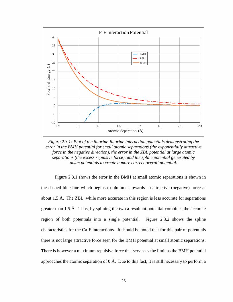
26
Figure 2.3.1: Plot of the fluorine-fluorine interaction potentials demonstrating the
error in the BMH potential for small atomic separations (the exponentially attractive
force in the negative direction), the error in the ZBL potential at large atomic
separations (the excess repulsive force), and the spline potential generated by
atsim.potentials to create a more correct overall potential.
Figure 2.3.1 shows the error in the BMH at small atomic separations is shown in
the dashed blue line which begins to plummet towards an attractive (negative) force at
about 1.5 Å. The ZBL, while more accurate in this region is less accurate for separations
greater than 1.5 Å. Thus, by splining the two a resultant potential combines the accurate
region of both potentials into a single potential. Figure 2.3.2 shows the spline
characteristics for the Ca-F interactions. It should be noted that for this pair of potentials
there is not large attractive force seen for the BMH potential at small atomic separations.
There is however a maximum repulsive force that serves as the limit as the BMH potential
approaches the atomic separation of 0 Å. Due to this fact, it is still necessary to perform a
-10
-5
0
5
10
15
20
25
30
35
40
0.9 1.1 1.3 1.5 1.7 1.9 2.1 2.3
Po
tenti
al E
ner
gy
(J)
Atomic Seperation (Å)
F-F Interaction Potential
BMH
ZBL
Spline

27
spline between the ZBL potential for small atomic separations and the BMH at larger
separations.
Figure 2.3.2: Plot of the calcium-fluorine interaction potentials demonstrating the error
in the BMH potential for small atomic separations (not as repulsive as it should be at
smaller separations), the error in the ZBL potential at large atomic separations (not as
attractive as it should be at larger separations), and the spline potential generated by
atsim.potentials to create a more correct overall potential.
The Ca-Ca interactions were a bit different. The BMH potential (as shown in Table
2.3.1) assumes there is no interaction between Ca atoms [36] due to the relatively large
atomic separations of the Ca atoms with other Ca atoms in the lattice. But this doesn’t
mean there is no interaction at all. In fact, there is still a potential that dominates at small
atomic separations that can be modeled by the ZBL potential, and a Coulombic potential
that dominates at larger separations. Because of this fact the initial input potential was
5
10
15
20
25
30
35
40
45
50
55
0.8 1 1.2 1.4 1.6
Po
tenti
al E
ner
gy
(J)
Atomic Seperation (Å)
Ca-F Interaction Potential
BMH
ZBL
Spline

28
simply the ZBL potential style and the simulation added in the Coulombic interactions as
part of the larger simulation.
2.3.2 LAMMPS input file setup
To move forward, several aspects of the simulation must be defined. These aspects
of the code are broken into sections, the initialization, atom definition, force field
definition, grouping, initialization, and equilibration. Within the initialization section of
the code the units, dimension, boundaries and atom style of the simulation are defined. For
this research the set of units used are called “metal” in LAMMPS. The units that are used
when setting the simulation units to “metal” are as follows:
Mass = grams/mole
Distance = angstroms (Å)
Time = picoseconds
Energy = eV
Velocity = angstroms/picosecond
Force = eV/Angstrom
Torque = eV
Temperature = kelvin (K)
Pressure = bars
Charge = multiple of electron charge (1.0 is a proton)
Electric Field = volts/angstrom

29
Density = gram/cc (simulation dimension)
Three dimensions are used with periodic boundaries in each dimension and the
“atom style” selected in LAMMPS was “charge”, denoting that the atom charges will need
to be considered through Coulombic interactions. The atom definition follows with the
specification of the lattice constant (5.444 Å for CaF2) and the placing of one lattice cell of
atoms which is then replicated, with each cell containing 8 full F atoms, 4, ½’s of Ca, and
8, ¼’s of Ca. For the damage cascade simulation, each unit cell is replicated 60 times in
each dimension, resulting in a 60x60x60 lattice simulation. The TDE simulation does not
require as many atoms and therefore was kept to 6 unit cell replications in each dimension.
Given that there are twelve atoms per lattice cell in CaF2 thus the damage cascade
simulation contained 2,592,000 atoms while the TDE simulation contained 2,592 atoms.
The LAMMPS atom definition section also contains the definition of mass and charge of
each atom type. The force field section is next where the potential files are specified.
Additionally, a hybrid potential file was created using the Coulombic interactions along
with the spline that was created earlier. This accounts not only for atomic interactions but
also charged interactions between each atom type. The next LAMMPS section follows
with the definition of regions and groups. The definition of regions and groups allows for
greater tailoring in tracking displacements. By defining a group of atoms one can extract
the collision information for only that group and thus save significant amounts of hard
drive space, because each time a dump is created information for nearly 2.6 million atoms
is recorded. In the initialization section, all compute commands are defined. These
commands define to computational aspects to be run during the simulation. Additionally,
the initial crystal velocity, time step, and output styles are set. The equilibration phase is

30
completed using NPT fix command in LAMMPS to set the appropriate temperature and
pressure in the simulation cell, and then the simulation is run for a defined number of time
steps. Example input files for both the TDE and damage cascade simulations are included
in Appendix A.
2.3.3 LAMMPS equilibration verification
As a general check for how the simulation is behaving after the equilibration is
completed, it is crucial to compare the density of the material and lattice constant with the
defined experimental values. The standard values for CaF2 are 3.18 g/cc for density, and
5.444 Å for the lattice constant. The equilibrated result from the cascade simulation
described here resulted in a density of 3.056 g/cc and Lattice Constant of 5.535 Å. These
values are within 10% of the standard values which is in general acceptable. However,
these parameters were further refined for the Threshold Displacement Energy (TDE)
calculations given that the simulation size could be much smaller for that purpose than for
a cascade simulation where some characteristics had to be relaxed for the simulation to be
completed in a reasonable amount of time. For the TDE simulations the density and lattice
constant were brought within 1% of the standard values resulting in a density simulated at
3.163 g/cc and a lattice constant of 5.473 Å.
2.4 LAMMPS Determination of TDE
2.4.1 Methodology for Determining TDE
The determination of the probabilistic TDE closely followed the theory, and used a
similar method, laid out by B. Cohen [29]. The determination of TDE involved a periodic
increasing of energy of a PKA for both Ca and F PKAs. At each PKA energy the

31
simulation ran for 5 picoseconds passed within the simulation, utilizing a NPT fix with a
randomized seed allowing the lattice to relax between each simulation and to ensure
randomized atomic interactions. Similar to the work completed by B. Cohen [29], this
simulation was designed to follow the Monte Carlo method in which the direction of the
PKA was randomized for a series of PKA energy values to obtain the results. Each
simulation was repeated a minimum of 1000 times in order to obtain a statistical value for
the probability of displacement for a particular PKA energy within the CaF2 lattice.
2.4.2 Calcium and Fluorine TDE Results
The results generated were compiled using Matlab within which an atom was
considered displaced if its total displacement was greater than 0.8 Å. From there a simple
determination of probability of displacement is generated and plotted. The data for the
displacement of a Ca atom in CaF2 is demonstrated in Figure 2.4.1. Similarly, the
probability of displacement was determined for F atoms in CaF2. The results of these
simulations are demonstrated in Figure 2.4.2.
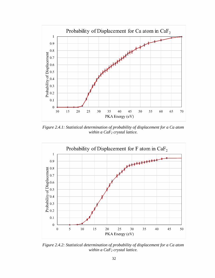
32
Figure 2.4.1: Statistical determination of probability of displacement for a Ca atom
within a CaF2 crystal lattice.
Figure 2.4.2: Statistical determination of probability of displacement for a Ca atom
within a CaF2 crystal lattice.

33
2.4.3 TDE Conclusions
To date, no current literature had shown the TDE of Ca and F atoms in CaF2 through
molecular dynamics and simulated statistical analysis. As such, the determination of these
values is a critical and key accomplishment of this work. Defining the TDE value as the
energy at which 50% of the atoms are displaced, as can be seen in Figures 2.4.2 and 2.4.3,
the statistical determination for the TDE of Ca, in a CaF2 lattice, yields a result of 32 eV.
Examining F in a CaF2 lattice yields a TDE of 20 eV. The result of this effort will
ultimately aid in further meso-scale simulation of radiation effects and will also serve to
set up a follow-on research study into a more detailed and complicated way of approaching
the meso-scale damage effects.
2.5 LAMMPS Damage Cascade
2.5.1 LAMMPS Damage Cascade Methodology
After the successful equilibration of the 60x60x60 simulation cell, the damage
simulation was set up. To do this the system is changed from NPT (constant Number of
particles, Pressure, and Temperature) to NVE (constant Number of particles, Volume, and
Energy, thus creating a system consistent with the microcanonical ensemble), but only for
the core of the overall lattice, with an exterior “buffer” layer retaining the NPT.
Throughout these simulations the damage cascade was watched by tracking the number of
vacancies and interstitial sites in the lattice over a period of time (generally about 20
picoseconds). Cascades were produced for a variety of PKA energies for both Ca and F
PKAs. To provide the most accurate results, a timestep function was inserted to analyze
the velocity of atoms in the material and the timestep was adjusted to ensure atoms were

34
not moving too fast. By doing this the integrity of the potential file is ensured. While the
original intention was to do this for a variety of angular momenta this was simply not
feasible given simulation times.
2.5.2 PKA Energy Calculation
The first step in modeling radiation damage using LAMMPS was to determine the
energy transferred to a PKA from a colliding neutron. Because of the nature of these
collisions, relativistic effects do not have to be considered but rather classical mechanics
can be utilized to calculate the velocity of a PKA atom. As previously discussed, many of
the collisions at these energies are inelastic, meaning that some kinetic energy is lost.
However, following the assumptions laid out in Section 2.2.5, a conservative
approximation can be made using classical mechanics assuming an elastic collision. This
assumption will of course mean that the kinetic energy calculated is likely slightly larger
than what will be experienced in nature, but this will provide a good estimate for the energy
transferred. Equation 7 shows the calculation of kinetic energy from the mass and velocity
of a particle,
𝐾𝐸 =1
2𝑚𝑣2 (Eq. 7)
where KE is the kinetic energy, 𝑚 is the particle mass, and 𝑣 is the velocity of said particle.
Rearranging the equation allows for calculation of velocity based on a given energy, shown
in Equation 8.
𝑣 = √2𝐾𝐸
𝑚 (Eq. 8)

35
In the case of a high energy (multiple MeV range) neutron it is likely kinetic that the energy
transferred to a PKA will be much greater than LAMMPS is able to simulate in this work
due to restrictions on simulation size. The PKAs and subsequent recoils may leave the
region contained in the calculation. Given this fact, the work presented here focuses on a
variety of PKA energies up to the maximum LAMMPS can handle with the current
simulation size, which are about 5000 eV for both Ca and F PKAs. For this setup, the PKA
velocity is converted to angstroms/picosecond. A table of PKA energies used for the
LAMMPS damage simulation are provided in Table 2.5.1.
Table 2.5.1: A table showing the velocity of a PKA in
Angstroms/Picosecond based on the desired PKA energy.
Desired E
(eV) Desired E (J)
Ca PKA
Velocity
(A/ps)
F PKA
Velocity
(A/ps)
5000 8.01x10⁻¹⁶ 1551.59 2253.60
2500 4.01x10⁻¹⁶ 1097.14 1593.54
1000 1.60x10⁻¹⁶ 693.89 1007.84
750 1.20x10⁻¹⁶ 600.93 872.82
250 4.01x10⁻¹⁷ 346.95 503.92
100 1.60x10⁻¹⁷ 219.43 318.71
75 1.20x10⁻¹⁷ 190.03 276.01
50 8.00x10⁻¹⁸ 155.16 225.36
40 6.41x10⁻¹⁸ 138.78 201.57
2.5.3 Calcium PKA Cascade Results
The energies in Table 2.5.1 were applied to Ca PKAs in a 2.5 million atom
simulation to generate radiation damage statistics. One primary statistic tracked over time
was the total number of lattice vacancies/interstitial sites in the simulation cell over a period
11 ps. In the time of the simulation, and consistent with radiation damage timeframes [41]

36
[42] [43] [44] [45], collisions due to high energy radiation have a very fast self-annealing
time, typically on the order of a few picoseconds. This is shown in Figure 2.5.1 where the
total lattice vacancies are plotted over time in picoseconds. It is seen here that the initial
self-annealing for these energies occurs very quickly and stabilizes into semi-permanent
damage after about 3-5 picoseconds depending on the PKA energy. It is a natural
assumption based on this plot that the initial self-annealing timeframe would increase at
higher energies. It is worth noting, as well, that the initial self-annealing for all simulations
was a nearly 90% recovery of the total initial number of vacancies.
Figure 2.5.1: Plot of lattice vacancies by Ca PKA with varying energies from 0 to 11
picoseconds.
In order to make this information more useful, a plot of persistent or semi-
permanent damage was created utilizing the number of vacancies that persisted in the
material 11 ps after the initial collision. Figure 2.5.2 demonstrates this subset of data. It

37
is clear, at least for the energies in this range of simulation, that the number of vacancies
produced by a single PKA at a specific energy increases linearly with the energy transferred
to the PKA. Naturally, there would be a limit to this, however that limit is not present in
this data set. Using this data an extrapolation can be made for higher energies based on the
equation given in Figure 2.5.2. This equation was determined through a curve fit of the
data.
Figure 2.5.2: Plot and trendline for persistent damage at 11 picoseconds after initial
self-annealing events. Equation and R2 value define the trendline.
2.5.4 Fluorine PKA Cascade Results
Similar to the Ca PKA simulation, the listed energies in Table 2.5.1 for F were
applied to F PKAs in a 2.5 million atom simulation to generate radiation damage statistics.
Again, the total number of lattice vacancies/interstitial sites in the simulation cell over a
period 11 ps. The results of this simulation are depicted in Figure 2.5.3.

38
Figure 2.5.3: Plot of lattice vacancies by F PKA with varying energies from 0 to 11
picoseconds.
Figure 2.5.3 shows similar behavior to the vacancies plotted for a Ca PKA. There
is an initial spike of damage that is not quite as dramatic as the spike produced by the Ca
PKA, which is expected given the smaller mass of the F PKA in comparison to the Ca
PKA. What was unexpected however was that the persistent damage due to PKAs of
different type but the same energy was very similar despite the initial damage spike from
the Ca PKA being about 28% greater. The F cascade had a recovery rate average of 85%
compared to the 90% recovery rate from the Ca cascade. It is worth noting that the damage
and recovery of the F PKA was much more erratic than that of the Ca PKA as is also clear
from the plots. Figure 2.5.4 takes the persistent damage at 11 ps and applies a trendline to
the data for an extrapolation of damage at higher energies. Similarly, an extrapolation was
made for higher energies based on the equation given in Figure 2.5.4. This equation was
determined through a curve fit of the data.

39
Figure 2.5.4: Plot and trendline for persistent damage from F PKA at 11 ps after
initial self-annealing events. Equation and R2 value define the trendline.
2.5.5 LAMMPS Cascade Modeling Conclusions
This simple analysis of a damage cascade within CaF2 due to both Ca and F PKAs
has produced some noteworthy results. It has been shown, for the PKA energy range
between 100 eV and 10 keV, that the persistent damage existing after the self-annealing of
the crystal structure is a linear function of the energy of the PKA. This suggests that when
entering the MeV range, as would be the result of PuBe source neutrons and fusion neutrons
seen later, that the higher the energy the more recognizable the damage should be. It
should be noted again that extrapolating to high energies is likely to produce error as it is
expected that, although the data suggests a linear relationship at very high PKA energies,
there is likely a limit to the amount of damage that can be incurred due to the physical
structure of the material.
In the experimental portion of this research the neutron energies that will be used are
within the average energy of 3-5 MeV for the NH-3 Neutron Howitzer, reactor energies of
a few MeV, and 2.5 MeV and 14.1 MeV for the Sandia Laboratory irradiations. It was
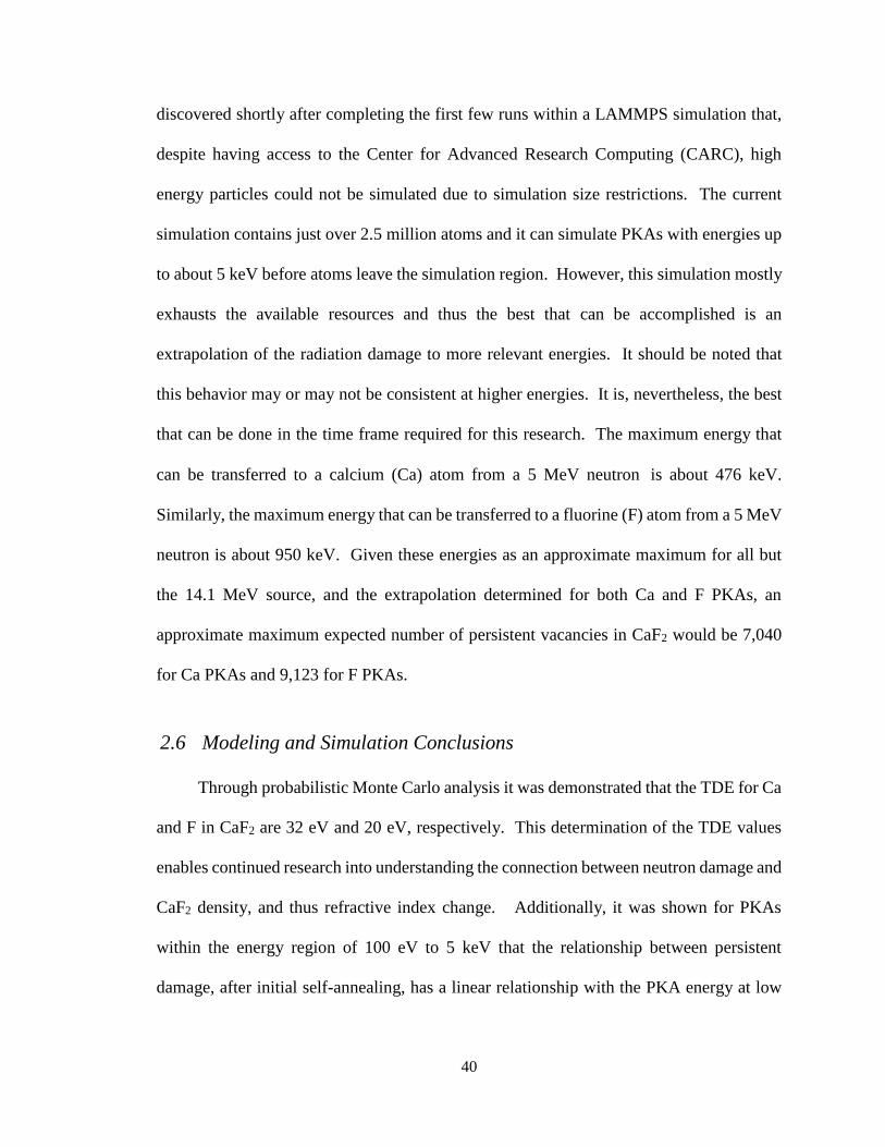
40
discovered shortly after completing the first few runs within a LAMMPS simulation that,
despite having access to the Center for Advanced Research Computing (CARC), high
energy particles could not be simulated due to simulation size restrictions. The current
simulation contains just over 2.5 million atoms and it can simulate PKAs with energies up
to about 5 keV before atoms leave the simulation region. However, this simulation mostly
exhausts the available resources and thus the best that can be accomplished is an
extrapolation of the radiation damage to more relevant energies. It should be noted that
this behavior may or may not be consistent at higher energies. It is, nevertheless, the best
that can be done in the time frame required for this research. The maximum energy that
can be transferred to a calcium (Ca) atom from a 5 MeV neutron is about 476 keV.
Similarly, the maximum energy that can be transferred to a fluorine (F) atom from a 5 MeV
neutron is about 950 keV. Given these energies as an approximate maximum for all but
the 14.1 MeV source, and the extrapolation determined for both Ca and F PKAs, an
approximate maximum expected number of persistent vacancies in CaF2 would be 7,040
for Ca PKAs and 9,123 for F PKAs.
2.6 Modeling and Simulation Conclusions
Through probabilistic Monte Carlo analysis it was demonstrated that the TDE for Ca
and F in CaF2 are 32 eV and 20 eV, respectively. This determination of the TDE values
enables continued research into understanding the connection between neutron damage and
CaF2 density, and thus refractive index change. Additionally, it was shown for PKAs
within the energy region of 100 eV to 5 keV that the relationship between persistent
damage, after initial self-annealing, has a linear relationship with the PKA energy at low

41
energies. This may be nonlinear at higher energies, but is beyond the scope of the current
simulation work.
42
Chapter 3: Measuring Refractive Index Change Optically
3.1 Overview
The basis of the research on relating refractive index change to neutron irradiations
is a technique for high precision index of refraction measurements invented by Professor
Jean-Claude Diels, who is leading the optics portion of this research. Through the
utilization of a nested-cavity mode locked laser, the change of refractive index in a material
can be measured with remarkable precision. Due to the nature of radiation damage caused
by neutrons, this technique is ideal for tracking changes due to neutron irradiation. Because
of the incident particle energy and momentum required to displace atoms in a lattice
leading to the change of refractive index, this technique ignores the effects of gamma
radiation; thus, this is a technique for gamma blind neutron characterization. This
technique is ideal for scenarios where other detectors/dosimeters are blinded by the number
of gamma rays in a system making it difficult to measure neutrons. This chapter will focus
on the theory, setup, and calibration of nested-cavity mode-locked laser designed
specifically for the purpose of measuring the change of refractive index in a material due
to neutron irradiation.
3.2 Optical Methods for Measuring Radiation Effects
A primary portion of this research includes making a measurement of the changes in
a crystal structure due to exposure to neutron radiation. The purpose of this research is to
demonstrate that this can be done by tracking the change in the refractive index of a crystal.
The general principle being that as radiation is absorbed in the crystal the density is
changed and thus the refractive index changes. This generalization is well established and
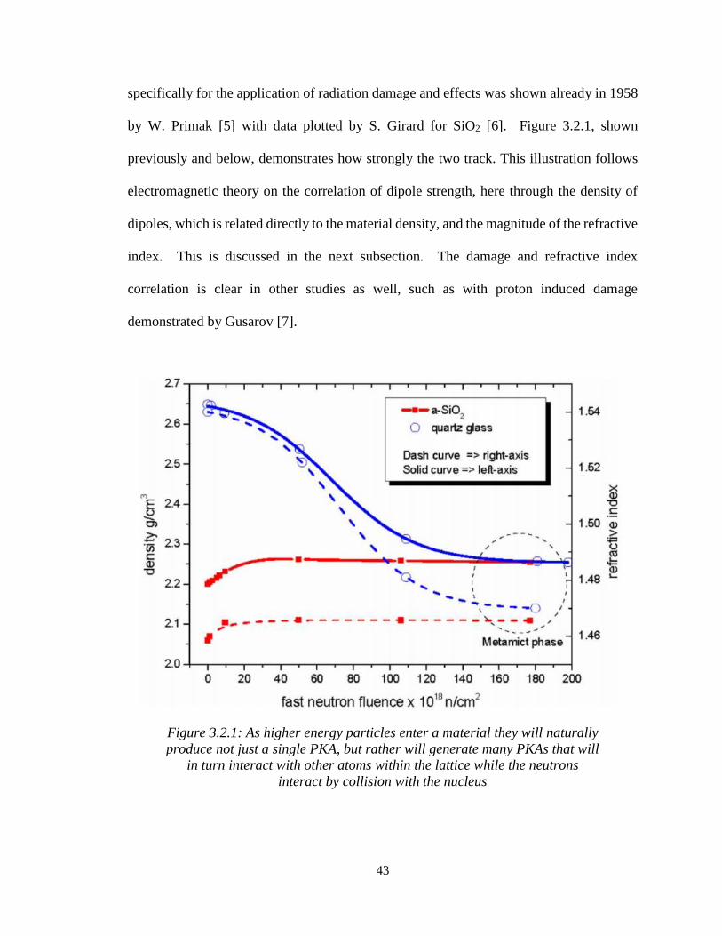
43
specifically for the application of radiation damage and effects was shown already in 1958
by W. Primak [5] with data plotted by S. Girard for SiO2 [6]. Figure 3.2.1, shown
previously and below, demonstrates how strongly the two track. This illustration follows
electromagnetic theory on the correlation of dipole strength, here through the density of
dipoles, which is related directly to the material density, and the magnitude of the refractive
index. This is discussed in the next subsection. The damage and refractive index
correlation is clear in other studies as well, such as with proton induced damage
demonstrated by Gusarov [7].
Figure 3.2.1: As higher energy particles enter a material they will naturally
produce not just a single PKA, but rather will generate many PKAs that will
in turn interact with other atoms within the lattice while the neutrons
interact by collision with the nucleus

44
Utilizing a nested mode-locked laser cavity it is possible to measure the change in
refractive index in a transparent material to a very precise degree. A brief proof of concept
for CaF2 was demonstrated to show that this technique provides very high precision
measurements of the change of refractive index [9]. The utilization of this optical
technique is of paramount importance to this work.
3.2.1 Refractive Index Overview
A critical piece of this research is the measurement of the change in refractive
index. To better understand this concept this section will outline a couple basic optical
science quantities of interest. It has been well established that when an electro-magnetic
(EM) wave passes through a material the molecules within the medium are polarized by
the oscillating electric field at the frequency of the propagating wave. The overall effect
of this is that the EM wave is slowed down in comparison to its free propagation in a
vacuum [46]. Each nonmagnetic dielectric medium has its own relative permittivity, 𝜀r
with respect to the permittivity of a vacuum, 𝜀o. When defined with the absolute
permeability, µo, the phase velocity of an EM wave can be defined by Equation 9.
𝑉𝑝 = 1
√𝜀µ (Eq. 9) [47]
Where 𝜀 = 𝜀𝑟𝜀𝑜 and µ = µ𝑟µ𝑜. Furthermore, the term phase refractive index is simply
the ratio of the speed of light in free space and a waves velocity inside a medium or as the
square root of the relative permittivity as shown in Equation 10.
𝑛𝑝 = 𝑐
𝑉≈ √𝜀𝑟 (Eq. 10) [46] [47]

45
The difficulty and the reason for the approximation in equation 10 is the fact that
the 𝑛 and 𝜀 are dependent upon frequency on the microscopic level. The fact that 𝑛 is
dependent on the wavelength of the EM wave is an effect termed dispersion. The index of
refraction 𝑛 is typically used to relate to the velocity of the oscillating wave, the phase,
𝑛𝑝 = 𝑣𝑝/𝑐 which should be specified as n phase, or 𝑛𝑝. Likewise, the velocity of the group
of waves, the wave bunch, may be related via 𝑛𝑔 = 𝑣𝑔/𝑐.
Since perfect monochromatic waves exist only in theory, one must consider the
velocity and index of a group of waves and how the dynamics change these quantities.
Thus, the wave packet (containing an oscillating field) travels at a velocity defined as the
group velocity shown in Equation 11,
𝑣𝑔 = 𝑑𝜔
𝑑𝑘 (Eq. 11)
where ω is the mean frequency of the oscillating field whose amplitude is modulated by
the varying field of frequency 𝑑𝜔 and 𝑑𝑘 is the wavevector within which the maximum
amplitude moves [46]. ω is defined as
𝜔 = 𝑉𝑘 = [𝑐
𝑛(𝜆)] [
2𝜋
𝜆] (Eq. 12) [46]
where n(λ) is written to explicitly show the dependence of the refractive index on the
wavelength of light passing through it. After solving for 𝑣 and differentiating to get 𝑣𝑔,
Equation 13 is obtained,
𝑉𝑔 =𝑐
𝑛−𝜆𝑑𝑛
𝑑𝜆
(Eq. 13) [46]

46
where
𝑛𝑔 = 𝑛 − 𝜆𝑑𝑛
𝑑𝜆 (Eq. 14) [46]
These four quantities will be the building blocks in comparing the repetition rate of the
FPE and the repetition rate of the laser cavity to determine the change in refractive index
of a crystal sample due to irradiation damage. Phase velocity relates with the movement
of the waves and the phase index of refraction, which is what is generally thought of when
discussing the index of refraction. The group velocity is more clear in a classical dynamics
sense when discussing movement of wave packets or bunches.
It has been shown already that refractive index and density are strongly correlated.
This effect is actually secondary, as the primary reason for the correlation is the fact that
density increases overall dipole density, or polarization density. This is a quantity of
classical electromagnetism defined as the vector field in a dielectric material that expresses
the density of induced electric dipole moments, where a dipole moment is the measure of
the separation of the negative and positive charges in a system. Generally, as the density
of a material increases or decreases (as is the case with neutron irradiation) the separation
of the charges changes in a direct correlation with the density. In the case of decreasing
density, the dipole moments become further apart (albeit on an extremely small scale but
still significant). The increased spacing of the dipole moments decreases the capacitance
and the polarization density which ultimately affect the permittivity of a medium. As stated
previously in Equation 10 the refractive index of a material is approximately equivalent to
the relative permittivity, 𝜀𝑟, of a material. The permittivity of a material is determined
using Equation 15,

47
𝜀𝑟 = 𝜀0 ∗ (1 + 𝜒) (Eq. 15)
where, 𝜀0, is the constant permittivity of free space and 𝜒 is the susceptibility, the macro-
scale quantity of polarizability. Thus, in summary the reason changes in refractive index
decreases with neutron irradiation is because neutron irradiation causes the atoms in a
structure to become more spread out that they normally are. As such, the dipole moments
are further separated causing a decrease in polarization density which in turn decreases the
relative permittivity of a material, which is the essential building block of the refractive
index.
3.2.2 Mode-locked laser cavity
The standard laser cavity is made up, minimally, of an optical resonator with two
end mirrors and a laser gain medium. There are typically many modes contained within
the optical resonator and the total output of the laser varies based on time, frequencies,
amplitudes and relative phases of the oscillating modes [48]. For waves within a cavity of
length L the allowed wavelengths, or frequencies, must satisfy the resonance condition of
the cavity in order to achieve mode-locking, which, in the frequency domain, creates a
frequency comb resembling a picket fence. The resolution of the resonance condition of
the cavity along with that of the inserted FPE are detailed in Section 3.3.1.
A laser is said to be mode-locked when “the oscillating modes are forced to
maintain equal frequency spacing with a fixed phase relationship to each other” with the
output over time varying in a well-defined manner [48]. A mode-locked laser is made to
produce extremely short pulse trains typically on the order of picoseconds with some in the
range of single digit femtoseconds [49].
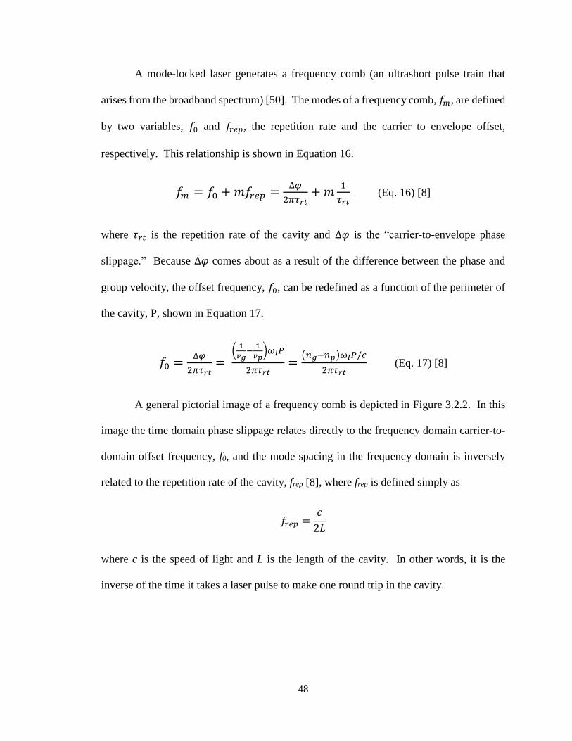
48
A mode-locked laser generates a frequency comb (an ultrashort pulse train that
arises from the broadband spectrum) [50]. The modes of a frequency comb, 𝑓𝑚, are defined
by two variables, 𝑓0 and 𝑓𝑟𝑒𝑝, the repetition rate and the carrier to envelope offset,
respectively. This relationship is shown in Equation 16.
𝑓𝑚 = 𝑓0 + 𝑚𝑓𝑟𝑒𝑝 =∆𝜑
2𝜋𝜏𝑟𝑡+ 𝑚
1
𝜏𝑟𝑡 (Eq. 16) [8]
where 𝜏𝑟𝑡 is the repetition rate of the cavity and ∆𝜑 is the “carrier-to-envelope phase
slippage.” Because ∆𝜑 comes about as a result of the difference between the phase and
group velocity, the offset frequency, 𝑓0, can be redefined as a function of the perimeter of
the cavity, P, shown in Equation 17.
𝑓0 =∆𝜑
2𝜋𝜏𝑟𝑡=
(1
𝑣𝑔−
1
𝑣𝑝)𝜔𝑙𝑃
2𝜋𝜏𝑟𝑡=
(𝑛𝑔−𝑛𝑝)𝜔𝑙𝑃/𝑐
2𝜋𝜏𝑟𝑡 (Eq. 17) [8]
A general pictorial image of a frequency comb is depicted in Figure 3.2.2. In this
image the time domain phase slippage relates directly to the frequency domain carrier-to-
domain offset frequency, f0, and the mode spacing in the frequency domain is inversely
related to the repetition rate of the cavity, frep [8], where frep is defined simply as
𝑓𝑟𝑒𝑝 =𝑐
2𝐿
where c is the speed of light and L is the length of the cavity. In other words, it is the
inverse of the time it takes a laser pulse to make one round trip in the cavity.

49
Figure 3.2.2: f0 in this figure is the frequency domain representation of the round
trip phase slippage, Δφ. The mode spacing is representative of the cavity repetition
rate, frep [8].
A remarkable and key feature of the frequency comb generated in a mode-locked
laser is that all present modes are evenly spaced according to the repetition rate (frep) of the
cavity. They are also shifted by the carrier envelope offset f0. Due to the fact that these
quantities completely characterize the frequency comb they can be manipulated in such a
way as to make “an ultra-sensitive measurement of a differential intracavity pulse shift”
[8]. Another fact that is crucial to this research is the ability to lock the group index of
refraction of the cavity, ng, utilizing the counter propagating pulses generated by the mutual
saturation of the pulse envelopes. Keeping ng constant or at least consistent throughout
experimentation allows for the isolation of np, the phase index of refraction. This
ultimately allows for the determination of the change in the phase index of a Fabry-Pérot
Etalon inserted into the cavity, which, for this work is a CaF2 sample.
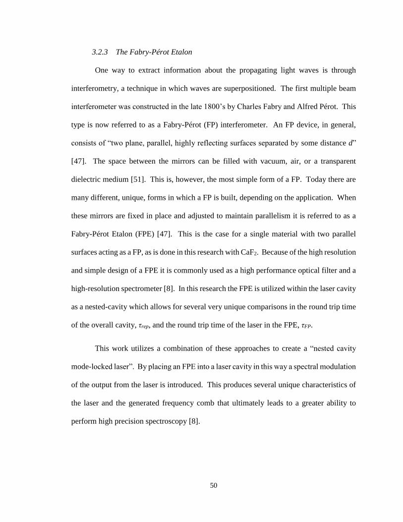
50
3.2.3 The Fabry-Pérot Etalon
One way to extract information about the propagating light waves is through
interferometry, a technique in which waves are superpositioned. The first multiple beam
interferometer was constructed in the late 1800’s by Charles Fabry and Alfred Pérot. This
type is now referred to as a Fabry-Pérot (FP) interferometer. An FP device, in general,
consists of “two plane, parallel, highly reflecting surfaces separated by some distance d”
[47]. The space between the mirrors can be filled with vacuum, air, or a transparent
dielectric medium [51]. This is, however, the most simple form of a FP. Today there are
many different, unique, forms in which a FP is built, depending on the application. When
these mirrors are fixed in place and adjusted to maintain parallelism it is referred to as a
Fabry-Pérot Etalon (FPE) [47]. This is the case for a single material with two parallel
surfaces acting as a FP, as is done in this research with CaF2. Because of the high resolution
and simple design of a FPE it is commonly used as a high performance optical filter and a
high-resolution spectrometer [8]. In this research the FPE is utilized within the laser cavity
as a nested-cavity which allows for several very unique comparisons in the round trip time
of the overall cavity, τrep, and the round trip time of the laser in the FPE, τFP.
This work utilizes a combination of these approaches to create a “nested cavity
mode-locked laser”. By placing an FPE into a laser cavity in this way a spectral modulation
of the output from the laser is introduced. This produces several unique characteristics of
the laser and the generated frequency comb that ultimately leads to a greater ability to
perform high precision spectroscopy [8].

51
3.2.4 Generation of High Frequency Pulse Trains
As previously mentioned, a basic mode-locked laser cavity generates singular pulses
in the time domain, separated in time by a factor determined by the length of the cavity. A
general representation of the basic time domain output of a simple mode-locked laser cavity
is depicted in Figure 3.2.3 where FM, depicts the focusing mirrors.
Figure 3.2.3: Demonstration of general function of a mode-locked laser cavity
generating singular pulses in the time domain at a rate determined by the cavity length.
The pumping laser enters from the left [8].
This pulse generation changes dramatically when inserting an FPE into the cavity.
By inserting an FPE at an angle into the basic cavity above, a pulse bunch is created similar
to the depiction in Figure 3.2.4.

52
Figure 3.2.4: Depiction of general function of a nested cavity mode-locked laser cavity
generating pulse bunches in the time domain at a rate determined by the cavity length.
The separation of the peaks within the bunch corresponds to the effective length of the
FPE [8].
The pulse bunch is due to the original cavity pulse from Figure 3.2.3 passing through
the FPE. Through a series of internal reflections many pulse peaks leave the FPE in
sequence; the intensity of the leading peak in the bunch is pushed back further in the bunch.
The expected pulse shape is a sawtooth pattern, as shown in Figure 3.2.4, but after several
passes with the intensity of each of the peaks diminished, a Gaussian shaped pulse bunch
is created, as in Figure 3.2.4. The Gaussian shape was determined to be correct by Koji
[52]. The generation and characterization of a high frequency pulse bunch within a nested-
cavity mode-locked laser are performed in great detail by K. Masuda in his dissertation
Intracavity coherent interaction of mode-locked pulse train with resonant medium [8]. This
work will be briefly reviewed here for the purpose of understanding its impact on precisely
measuring the change of refractive index. Short pulses passing through a FPE, with pulse
widths smaller than the round trip reflection time within the FPE, are transformed into
pulse trains by this internal reflection, as in Figure 3.2.5.
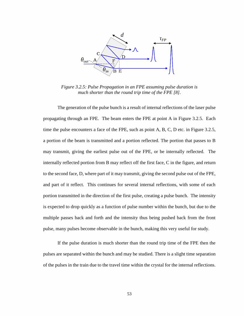
53
Figure 3.2.5: Pulse Propagation in an FPE assuming pulse duration is
much shorter than the round trip time of the FPE [8].
The generation of the pulse bunch is a result of internal reflections of the laser pulse
propagating through an FPE. The beam enters the FPE at point A in Figure 3.2.5. Each
time the pulse encounters a face of the FPE, such as point A, B, C, D etc. in Figure 3.2.5,
a portion of the beam is transmitted and a portion reflected. The portion that passes to B
may transmit, giving the earliest pulse out of the FPE, or be internally reflected. The
internally reflected portion from B may reflect off the first face, C in the figure, and return
to the second face, D, where part of it may transmit, giving the second pulse out of the FPE,
and part of it reflect. This continues for several internal reflections, with some of each
portion transmitted in the direction of the first pulse, creating a pulse bunch. The intensity
is expected to drop quickly as a function of pulse number within the bunch, but due to the
multiple passes back and forth and the intensity thus being pushed back from the front
pulse, many pulses become observable in the bunch, making this very useful for study.
If the pulse duration is much shorter than the round trip time of the FPE then the
pulses are separated within the bunch and may be studied. There is a slight time separation
of the pulses in the train due to the travel time within the crystal for the internal reflections.

54
When the pulses are sufficiently short, no interference occurs between pulses and the delay
between pulses can be written as:
𝜏𝑓𝑝 =2𝑛𝑝𝑑 cos 𝜃𝑖𝑛
𝑐 (Eq. 18) [8]
where 𝜏𝑓𝑝is the round trip time of the FPE. Each subsequent reflection is displaced slightly
from the optical axis; the displacement is a function of FPE angle. The repetition rate of
the overall cavity will change with angle as well. Moreover, at a certain angle, depending
on the type and thickness of the FPE used the nested-cavity mode-locked laser will
transition to single-pulse mode-locking due to the fact that at this point the cavity loss of
the multiply reflected pulses exceeds the gain.
Utilizing a fused-silica FPE, Masuda demonstrated that a standard nested-cavity
mode-locked laser generates a somewhat Gaussian shaped pulse bunch [8]. A simulation
of this is demonstrated by J. Hendrie who has shown that, due to the internal reflections in
an FPE, along with the gains and losses of the cavity a Gaussian pulse bunch is generated.
Due to reflection losses, this simulation for fused silica demonstrated an attenuation by a
factor of (0.04)2 [52] for each successive pulse reflection passing through the FPE.
With regard to the round-trip time of the cavity, this pulse bunch travels in a similar
fashion to the pulse in a standard mode-locked laser. This behavior is shown in Figure
3.2.6 where a partially resolved intensity profile of individual pulses is demonstrated [8].
In this example, the cavity repetition time of 6.4 ns corresponds with a repetition rate of
156 MHz and the FPE repetition time of 148 ps corresponds with a repetition rate of 6.76
GHz.

55
Figure 3.2.6: The output of a nested-cavity mode-locked
laser (bottom) as it is compared to that of an identical
cavity not containing an FPE (top) [8].
The frequency space representation of the simple mode locked laser pulsing without
the FPE is a frequency comb, as in the top of Figure 3.2.7. When measuring the frequency
space representation with the FPE, with pulse bunches, the frequency comb has an
envelope, as seen in the bottom of Figure 3.2.7.

56
Figure 3.2.7: The RF spectrum of a single mode-locked laser
(Top) containing no FPE. The RF spectrum of a nested-cavity
mode-locked laser (Bottom) with 15 mm fused silica FPE.
The repetition rate of both lasers were set to the same value.
The inset plot (Middle) demonstrates train shift resulting from
the formation of pulse bunches [8].
The width of the envelope pictured in the bottom of Figure 3.2.7 is determined by
the time domain extension of the pulse bunch. The frequency offset shown in the inset
figure in Figure 3.2.7 is a consequence of the differences in velocity of the pulse bunch
envelope and the individual pulses. For this example, from our research group's work in
[44], the center of the envelope is at 6.76 GHz, following the FPE behavior, and the spacing
between teeth of the comb is 0.156 GHz, following the cavity behavior.
In the current work the FPE utilized is CaF2, with a thickness of 15 mm and a
diameter of 25.4 mm and 20.3 mm depending on the experiment. The thickness is the only
parameter of great importance here as that determines where in the frequency space the
representation of the pulse bunches will appear. The more thin an FPE is the shorter the

57
FPE repetition rate and the higher the frequency will be. With frequency considerations
and the 27 GHz spectrum analyzer we were able to acquire for this research, a 15 mm
thickness was deemed appropriate. A picture of the standard FPE utilized in this work is
shown in Figure 3.2.8.
Figure 3.2.8: Picture of a CaF2 FPE utilized in this
research. This FPE is the 20.3 mm diameter sample.
3.3 Measuring the Change of Refractive Index Optically
3.3.1 Coupling Resonance Conditions of an FPE in a nested-cavity
As discussed earlier the resonance condition is an equation that must be satisfied in
order to achieve mode-locking in any laser cavity. However, in a nested cavity such as the
one discussed in this work, to achieve mode-locking the resonance condition of the FPE
and the laser cavity must be satisfied at the same time. These two resonance conditions
are [52]:

58
2𝜔0𝐿𝑛𝑝−𝑙
𝑐= 2𝜋𝑁𝑙 (Eq. 19)
2𝜔0𝑑𝑛𝑝−𝑓𝑝 cos 𝜃
𝑐= 2𝜋𝑁𝑓𝑝 (Eq. 20)
where 𝜔0 is the mode frequency, L and d are the lengths of the laser cavity and the
thickness of the FPE, respectively, 𝑛𝑝−𝑙 and 𝑛𝑝−𝑓𝑝 are the phase refractive indices of the
cavity and the FPE, respectively, and 𝑁𝑙 and 𝑁𝑓𝑝 are integer values, the mode numbers for
the resonance of the cavity and FPE, respectively. Each of these is a function of the
conditions of the system, the laser cavity length, and the PFE thickness and angle. When
the ratio of the two conditions is compared, it leads to the resonance condition of the
combined FPE-laser cavity system [52]:
𝐿
𝑑 cos 𝜃=
𝑛𝑝−𝑓𝑝𝑁𝑙
𝑛𝑝−𝑙𝑁𝑓𝑝 (Eq. 21)
Remarkably, this condition is satisfied passively in a free-space configuration described in
[52]. The round trip travel time for the FPE (𝜏𝑓𝑝) and the cavity (𝜏𝑙) are given by
𝜏𝑓𝑝 =2𝑑𝑛𝑔−𝑓𝑝 cos 𝜃
𝑐 (Eq. 22)
𝜏𝑙 =2𝐿𝑛𝑔−𝑙
𝑐 (Eq. 23)
where 𝑛𝑝−𝑓𝑝 is the phase index of refraction of the FPE. Also, 𝑛𝑔−𝑐 and 𝑛𝑔−𝑓𝑝 are the
group indices of refraction of the laser cavity and the FPE, respectively. The inverse of
these round trip times are the low (𝜈𝑙) and high (𝜈𝑓𝑝) frequency components, respectively,

59
described above. Taking the ratio of the frequencies and substituting L from equation 21
gives:
ℛ =𝜈𝑙
𝜈𝑓𝑝=
𝑐𝑛𝑝−𝑙𝑁𝑓𝑝
2𝑑 cos 𝜃𝑛𝑝−𝑓𝑝𝑁𝑙𝑛𝑔−𝑙 2𝑑𝑛𝑔−𝑓𝑝 cos 𝜃
𝑐=
𝑛𝑝−𝑙𝑛𝑔−𝑓𝑝
𝑛𝑔−𝑙𝑛𝑝−𝑓𝑝
𝑁𝑓𝑝
𝑁𝑐 (Eq. 24)
Equation 24 is also referred to the LF/HF ratio. Unlike the previous equations, the
ratio is not explicitly dependent on the FPE thickness or angle or the cavity length, though
those play into the particular resonance condition integers, but on the various refractive
indices and resonance modes. While the modes, 𝑁𝑓𝑝 and 𝑁𝑐, are integers, the ratio 𝑁𝑓𝑝 /
𝑁𝑐 is a constant but not necessarily an integer [52]. Additionally, 𝑛𝑔−𝑓𝑝, 𝑛𝑔−𝑙, 𝑛𝑝−𝑙, the
group index of the FPE, the group index of the laser cavity, and the phase index of the laser
cavity, respectively, do not vary significantly compared to the expected change in 𝑛𝑝−𝑓𝑝
due to irradiation. This allows for the isolation of 𝑛𝑝−𝑓𝑝 and ultimately a determination of
the change of the phase index of refraction in the FPE.
3.3.2 Mode-Locked Laser Cavity Pulse Width
A mode-locked laser cavity depends on a number of cavity characteristics, s
discussed in the theory Section 3.2.2. One such characteristic needed to ensure optimal
operation with a Fabry-Pérot Etalon inserted into the cavity is the laser pulse width in time.
Minimizing the laser cavity pulse width has been a subject of experimentation for several
decades resulting in some astonishing feats [49]. To date there have been publications of
pulses smaller than 1 femtosecond [53]. For this work, however, single picosecond range
pulses will suffice. A one picosecond pulse corresponds to a length of approximately 0.3
mm in a vacuum. The thickness of the CaF2 FPE samples in this research is 15 mm. In
order to produce stable frequency combs, the single length of a pulse must be able to be
60
contained within the FPE, leading to a more relaxed pulse length requirement. Laser beam
pulse widths can be measured precisely utilizing technique developed by J.C. Diels referred
to as an interferometric autocorrelation [54] [55]. Figure 3.3.1 demonstrates the results of
this type of autocorrelation with the figure scaled to clearly depict the pulse width of the
linear laser cavity used in this research before the insertion of the FPE.
Figure 3.3.1: Plot of an Interferometric Autocorrelation of the linear
laser cavity without an FPE operating at 7.01W and 790nm.
Figure 3.3.1 demonstrates a pulse width of less than 2 picoseconds prior to FPE
insertion. This measurement meets the requirements for this research and provides a
stepping point for FPE insertion and a repeat of the pulse width measurement with the FPE
inserted. Figure 3.3.2 demonstrates the results of the autocorrelation with multiple pulses.

61
Figure 3.3.2: Autocorrelation plot showing the multiple pulse train caused by the
insertion of the CaF2 FPE insterted at an internal angle of 8 mrad into a linear
laser cavity operating at 7.01W and 790nm.
Notice in Figure 3.3.2 that the separation in picoseconds corresponds to the
repetition rate of the FPE, which is approximately 145.75 ps, corresponding to a frequency
of 6.861 GHz. This is mirrored in the frequency comb separation when viewing the
frequency space representation of the pulse train. The addition of the FPE to the cavity
necessarily changes some of the cavity characteristics and it was appropriate to run another
autocorrelation after FPE insertion to ensure that the pulse width is still within a
manageable range. A close-up view of the autocorrelation conducted after the FPE was
added into the laser cavity is shown in Figure 3.3.3.

62
Figure 3.3.3: Enhanced plot central pulse of an Interferometric
Autocorrelation of the linear laser cavity operating at 7.01W, 790nm,
with a CaF2 FPE inserted at an internal angle of 8 mrad.
Figure 3.3.3 shows that with the insertion of the FPE the pulse width has decreased
slightly and is approximately around 1 to 1.5 picoseconds. This is still well within the
necessary range and thus the next aspect of the research commenced with the examination
of the pulse bunches in the time domain and frequency space.
3.3.3 Nested-Cavity Pulse Bunches and Frequency Combs
The time domain output of this setup is represented well in Figure 3.3.4 showing
two laser pulses within the cavity occurring about 8.5 ns apart corresponding to a frequency
value for the repetition rate of the laser cavity of approximately 117.582 MHz. Another
point worth noting in this image is the separation between each peak corresponds to the
repetition rate within the Fabry-Pérot which directly depends on the refractive index.

63
Tracking the change in both quantities is what allows for the high precision measurements
of change in refractive index to be accomplished.
Figure 3.3.4: Time domain representation of two pulse bunches within the laser
cavity setup. The inset plot shows a close up of the first pulse bunch.
Figure 3.3.5: Frequency domain representation of the pulse bunches within the
laser cavity, featuring well defined frequency combs whose central peaks
correspond directly to the repetition rate of the FPE.

64
The frequency domain output of this setup is represented in Figure 3.3.5 which now
shows the frequency combs characteristic of a mode locked laser with the envelopes caused
by the addition of the FPE. The separation of the center peak of each envelope is equal to
the repetition rate (referenced in Section 3.3.1 as 6.861 GHz) of the pulse from the FPE in
frequency space. When the either the angle or length of the laser cavity is changed while
keeping everything else constant the location of the observed peaks to the right and left of
the center peak in the bunch move further away from the central peak at increasing rates
depending how far the observed peak is away from the central peak. This also changes
with a swelling of the crystal and thus a change in phase refractive index. This allows for
comparison of a pre- and post-irradiated sample. As a result, when comparing the pre- and
post-irradiated sample as the FPE angle or cavity length are changed the ratio of the
frequency ratios will correspond directly to the change in refractive index.
3.3.4 Quantifying the Change in Refractive Index
The next vital step to this research is the ability to utilize the low-frequency to high-
frequency ratio in Equation 24 to extract the change in the refractive index of a material
after a sample is irradiated. This can be accomplished only when keeping all parameters
(primarily the cavity gain and losses) in the cavity constant except for 𝑛𝑝,𝑓𝑝, the phase
refractive index of the FPE. In order to extract this quantity a comparison of the pre-
irradiated sample and the post irradiated sample must be performed. The frequency ratio
can then be compared before and after crystal damage occurs to measure the change of
refractive index in the FPE. This comparison, shown below in Equation 25 in a ratio of
the LF/HF ratios from Equation 24, is to be called a super ratio for this work. This is a
function only of the phase index of refraction of the FPE - the crystal sample - if all other

65
values can be kept constant. The super ratio for crystal 0 and 1 (for example representing
pre- and post-irradiation ratios) then is expressed as
ℝ =ℛ0
ℛ1=
𝑛𝑝,𝑓𝑝,1
𝑛𝑝,𝑓𝑝,0=
𝑛𝑝,𝑓𝑝,0+Δ𝑛𝑝,𝑓𝑝
𝑛𝑝,𝑓𝑝,0= 1 +
Δ𝑛𝑝,𝑓𝑝
𝑛𝑝,𝑓𝑝,0 (Eq. 25)
This super ratio can also be utilized to correct for long term shifts such as thermal
effects on cavity length and assess the error in such a correction as it is applied to the super-
ratio of the pre- and post-irradiated sample.
The desired quantity to be extracted is Δ𝑛𝑝,𝑓𝑝, the change in the refractive index of
a material. The change in refractive index can then be extracted by adjusting Equation 25
to give:
Δ𝑛𝑝,𝑓𝑝 = (ℝ − 1) 𝑛𝑝,𝑓𝑝,0 (Eq. 26)
3.3.5 Angular and Cavity Length Dependence
The super-ratio can be taken in a point by point comparison of ratios between two
samples. There are two primary ways to keep all parameters (except 𝑛𝑝,𝑓𝑝,1) unchanged
while taking several measurements. This can be accomplished with an angle scan, depicted
in Figure 3.3.6, in which the overall length of the laser cavity is kept constant while the
internal angle of the FPE is gradually changed from a relatively high angle (about 20 mrad
for CaF2) to the zero angle of the FPE at which point mode-locking in the laser cavity does
not exist. The scan can be taken from some high angle, through zero, which is extremely

66
clear in the laser behavior, all the way to the same relative point on the other side of the
zero angle, but this is not necessary to make the comparison required by this research.
Figure 3.3.6: A simplified depiction of a laser cavity emphasizing the
constant cavity length requirement for an angle scan to determine the
refractive index change of an FPE.
In a similar fashion, the other method of obtaining the necessary parameter
consistency while taking several different data points, is varying the length of the laser
cavity while keeping the FPE angle constant. A difficulty in this measurement is ensuring
that the angle of the scan is always the same between trials. When removing the sample
from the laser cavity for irradiation it is difficult and improbable that when a sample is
placed back in the cavity it will be at the identical location and angle as it was previously.
In order to ensure repeatability to an acceptable degree of error an angle scan must first be
completed in order to determine the zero angle of the FPE. Upon completion of this step
the required angle position can be calculated. At this point the angle is only subject to the
error of the motor driving the micrometer screw that sets the angle of the FPE, which has
a quoted bi-directional repeatability of < ±1.5 µm, corresponding, in this experimental
setup to a tilt angle of ±0.275 mrad [56]. A simplified depiction of a cavity length scan is
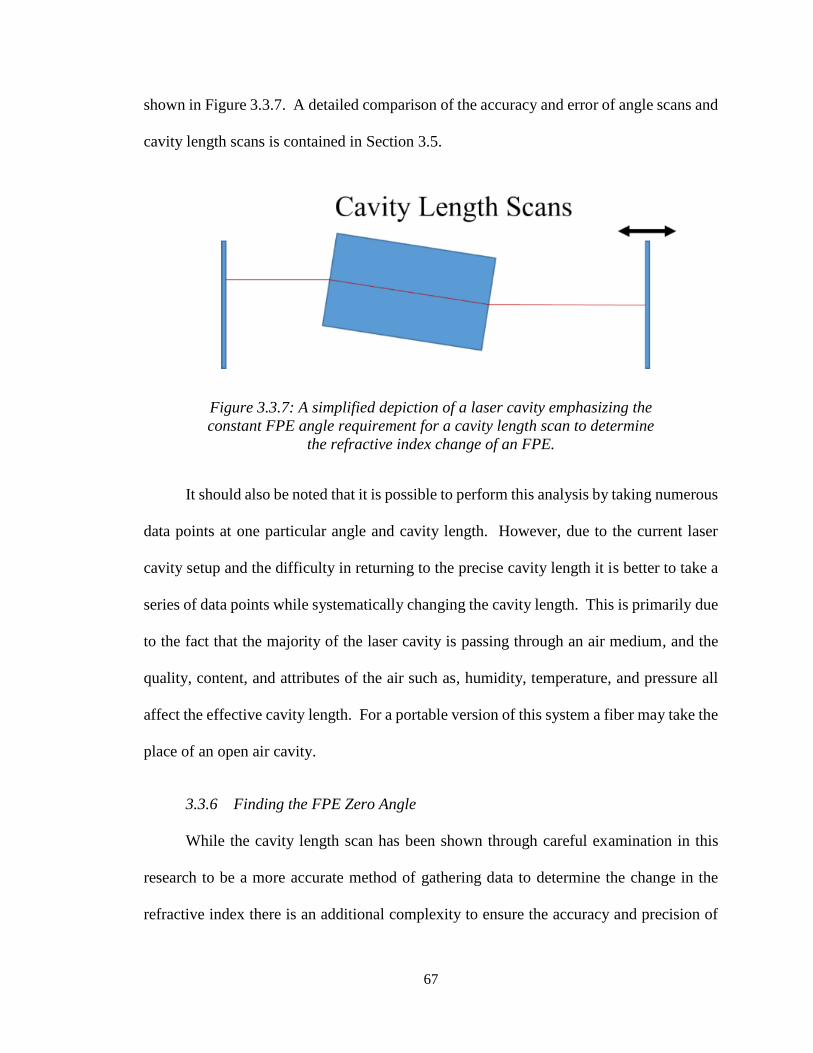
67
shown in Figure 3.3.7. A detailed comparison of the accuracy and error of angle scans and
cavity length scans is contained in Section 3.5.
Figure 3.3.7: A simplified depiction of a laser cavity emphasizing the
constant FPE angle requirement for a cavity length scan to determine
the refractive index change of an FPE.
It should also be noted that it is possible to perform this analysis by taking numerous
data points at one particular angle and cavity length. However, due to the current laser
cavity setup and the difficulty in returning to the precise cavity length it is better to take a
series of data points while systematically changing the cavity length. This is primarily due
to the fact that the majority of the laser cavity is passing through an air medium, and the
quality, content, and attributes of the air such as, humidity, temperature, and pressure all
affect the effective cavity length. For a portable version of this system a fiber may take the
place of an open air cavity.
3.3.6 Finding the FPE Zero Angle
While the cavity length scan has been shown through careful examination in this
research to be a more accurate method of gathering data to determine the change in the
refractive index there is an additional complexity to ensure the accuracy and precision of

68
the measurement. This complexity is the determination of the Zero Angle. The Zero Angle
of the FPE is the point at which the laser will stop mode-locking in a cavity due to the beam
interference caused by the extremely small internal angle of the FPE. While in a typical
laser cavity mode-locking will actually stop at a series of internal angles surrounding the
zero angle it is the actual zero angle that must be determined accurately in order to
determine the actual position of the zero angle. Fortunately, there are several ways to
accomplish this. The method settled on for this research utilizes a photodetector to
determine the strength of the laser beam. Figure 3.3.8 demonstrates the placement of the
photodetector outside of the cavity.
Figure 3.3.8: Demonstration of the position of the Photodetector
(Det1) with respect to the standard laser cavity comprised of two
focusing mirrors (M1) and a Fabry-Pérot Etalon (FP).
In order to increase accuracy of zero angle determination a photodetector is placed
at a position as far from the cavity as possible to allow for greater precision measuring the
reflections from the FPE as they begin to overlap at small internal angles. When
approaching zero angle the response the photodetector will continue to get stronger until
the internal reflections of the FPE begin to interact. Due to their interaction, the intensity
of the light will diminish locally creating a valley in the detected voltage. Zero Angle is

69
determined to be at the local minimum of the detected voltage from the photodetector.
Figure 3.3.9 provides a generalized representation of this data.
Figure 3.3.9: Generalized ideal depiction of the photodetector data as
the internal angle of the FPE is adjusted from a high positive internal
angle to a high negative internal angle.
It is only after performing a long scan through FPE internal angles that the zero
angle can be determined. After the zero angle in determined, then a cavity length scan can
be performed by utilizing the zero angle to determine the position of the internal angle of
interest and setting the FPE to the desired angle.
3.3.7 Reproducing Cavity Length Range
Although it is not quite as crucial it is certainly important to ensure that the cavity
length remains similar between all experimental results. The necessity of this is diminished
by performing cavity length scans instead of performing scans at only one specific cavity
length. At the start of each cavity length scan the repetition rate of the cavity is compared
to that of a previous scan. This ensures that the cavity length is similar between all
measurements.

70
3.4 Experimental Setup
As discussed in the theory Section 3.2, the setup for measuring refractive index
change in a material consists of a laser cavity containing two parallel end mirrors, a gain
medium, and a FPE. A more detailed rendering with the additional components included
in this setup is shown in Figure 3.4.1.
Figure 3.4.1: A detailed rendering of the laser cavity setup for measuring
refractive index change in a material, where M1 is the focusing mirror, P1 and
P2 are prisms, MQW is the Multiple Quantum Well, F1 is the Focussing Lense,
Det1 and Det2 are the Low Frequency and High Frequency detectors, and FP is
the Fabry-Pérot Etalon.
Figure 3.4.1 shows more components than discussed previously in the theory
sections. This includes the presence of a multiple quantum well (MQW), an end mirror,
two prisms, two focusing mirrors, and two detectors. The MQW acts as one of the two end
mirrors and due to the associated energy band gaps of the material acts to stabilize the laser

71
beam within the cavity. The prisms act to decrease the dispersion of the light within the
cavity, allowing only a narrow wavelength band along the correct path, also aiding in
stability the laser beam as well as the frequency combs in frequency space. The focusing
mirrors focus the beam into the gain medium. Lastly, one detector is used to measure the
repetition rate of the cavity and one is utilized to measure the repetition rate of the FPE.
3.5 Laser Cavity Calibration and Repeatability Measurements
3.5.1 Cavity Length Scans vs. Angle Scans
In order to be able to quantitatively state that the refractive index has changed, both
stability and noise must be assessed. A set of experiments were completed to measure the
repeatability of the data taken using unirradiated crystals in preparation for the irradiated
sample measurements. The experiments consisted of both cavity length scans and FPE
angle scans. Four trials consisting of four scans each were completed. In between each
trial the CaF2 FPE was removed from its holder in the laser cavity and placed back in a few
moments later to test placement repeatability and associated changes in the data. For true
irradiation measurements, the samples will need to be removed in order to be taken to be
irradiated and thus this measurement is a critical one in demonstrating repeatability. In
addition, this set of experiments was completed over a period of 2-3 different days to track
the noise due to environmental changes from day to day.
The angle scans were completed varying the internal angle of the FPE from about
+8 mrad to -4 mrad, where the zero angle, previously discussed, is defined as 0 mrad. The
following figures demonstrate a function of the frequency ratios, where the repetition rate
of the FPE in Hz is divided by the repetition rate of the laser cavity in Hz (recall Equation

72
24). In order to assess the stability more clearly for this particular experiment the LF/HF
frequency ratio was inverted to HF/LF. (This is the only experiment which required the
inversion of the frequency ratio and as such when the frequency ratio is quoted in the
remainder of this work it generally refers to the repetition rate of the cavity divided by the
repetition rate of the FPE). The ratio was then multiplied by the ratio of the number of
modes in the FPE to the number of modes in the cavity and is subtracted by one in order to
more clearly address the stability of the data. By multiplying out the ratio of modes the
only values remaining are the ratio of the phase and group indices for the cavity and the
FPE. Because the ratio of the indices will be a value minimally greater than one by
subtracting one the assessment of stability is much more clear. The equation is presented
below:
1
ℛ
𝑁𝑓𝑝
𝑁𝑐− 1 =
𝑛𝑔,𝑐𝑛𝑝,𝑓𝑝
𝑛𝑝,𝑐𝑛𝑔,𝑓𝑝
𝑁𝑐
𝑁𝑓𝑝
𝑁𝑓𝑝
𝑁𝑐− 1 =
𝑛𝑔,𝑐𝑛𝑝,𝑓𝑝
𝑛𝑝,𝑐𝑛𝑔,𝑓𝑝− 1 (Eq. 27)
The figures in this section have the y axis label “Inverted Frequency Ratio – 1” in
reference to Equation 24. This step would not be done in the case of Equation 25 because
the order is intrinsically divided out of the equation when taking the super-ratio. Figure
3.5.1 shows the average ratio of each trial point by point, plus and minus the standard
deviation of each respective trial from March 8, 2016. The four separate colors represent
the average of each of the four separate trials demonstrating the variation in each of the
trials, after which the sample was removed and placed back into the cavity to test placement
stability. Figure 3.5.2 shows the overall average ratio for the four trials of four angle scans
each on March 8, 2016, presented point by point in blue plus and minus the overall standard
deviation with boundaries in red.

73
Figure 3.5.1: Frequency ratio data for each of four separate angle scan trial
on March 8, 2016, each represented by a different color and associated dotted
line representing the standard deviations of each point in the trial.
Figure 3.5.2: Overall average frequency ratio data with overall standard
deviation from angle scans on March 8, 2016.

74
Due to the instability of the detection of the repetition rate around the zero angle
statistical analysis for the angle scans had to be completed in the region from about 2 mrad
to 8 mrad to accurately portray the statistical data. Figure 3.5.3 shows a close up of these
angles from Figure 3.5.2.
Figure 3.5.3: Close up of Figure 3.5.2 region of interest with statistical analysis
boasting standard deviation of 3.869x10⁻⁴.
Figure 3.5.4 shows the average ratio of each trial point by point, plus and minus the
standard deviation of each respective trial from March 9, 2016. The four separate colors
represent the average of each of the four separate trials demonstrating the variation in each
of the trials, after which the sample was removed and placed back into the cavity to test
placement stability. Figure 3.5.5 shows the overall average ratio for the four trials of four
angle scans each on March 9, 2016, presented point by point in blue plus and minus the
overall standard deviation with boundaries in red.

75
Figure 3.5.4: Frequency ratio data for each of four separate angle scan trial
on March 9, 2016 each represented by a different color and associated dotted
line representing the standard deviations of each point in the trial.
Figure 3.5.5: Overall average frequency ratio data with overall standard
deviation from angle scans on March 9, 2016.

76
Figure 3.5.6: Close up of Figure 3.5.5 region of interest with statistical analysis
boasting a standard deviation of 2.781x10⁻⁴.
Again, because of the instability of the detection of the repetition rate around the
zero angle statistical analysis for the angle scans had to be completed in the region from
about 2 mrad to 8 mrad to accurately portray the statistical data. Figure 3.5.6 shows a close
up of these angles from Figure 3.5.5. The experiment from March 8 produced data with a
3.869x10⁻⁴ standard deviation while the experiment from March 9 gave a 2.781x10⁻⁴
standard deviation.
On March 9, 10, and 11, 2016, cavity length scans were performed for a similar
statistical analysis while keeping the FPE internal angle constant at 4 mrad. The results of
this experiment are shown in Figure 3.5.7 to Figure 3.5.12. The overall cavity length was
changed from +0.5 mm longer to -0.5 mm shorter than the cavity length at which the angle
scans were performed. Figure 3.5.7 shows the results for 16 data runs averaged into 4
separate trials for data taken on March 9. Figure 3.5.8 shows the overall average and

77
standard deviation of the data from the 4 trials shown in Figure 3.5.7. Figure 3.5.9 shows
the results for 16 data runs averaged into 4 separate trials for data taken on March 10.
Figure 3.5.10 shows the overall average and standard deviation of the data from the 4 trials
shown in Figure 3.5.9. Figure 3.5.11 shows the results for 16 data runs averaged into 4
separate trials for data taken on March 11. Figure 3.5.12 shows the overall average and
standard deviation of the data from the 4 trials shown in Figure 3.5.11.
Notably, in Figure 3.5.7 there was considerable instability in the measurements
when the cavity length was changed in the positive direction above zero. The spikes in all
of these plots represent a data dropout point in which either the frequency peaks
representing the repetition frequency of the cavity or the repetition frequency of the FPE
went to zero because of the signal drop out. Thus, the program selected the highest peak
in the region leading to the instability. This instability can be corrected and was in the case
of the measurements completed on March 10 and March 11, demonstrated by the
significant lack of data variation. All of these plots for cavity length scans were plotted in
the same axis range as the angle scans for comparison.

78
Figure 3.5.7: Frequency ratio data from four separate trials on March 9,
2016 with an overall cavity length change of 1 mm.
Figure 3.5.8: Overall average frequency ratio data (all four trials) with
overall standard deviation from cavity length scans on March 9, 2016.
Statistical analysis shows a standard deviation of 3.066x10⁻⁵

79
Figure 3.5.9: Frequency ratio data from four separate trials on March 10,
2016 with an overall cavity length change of 1 mm.
Figure 3.5.10: Overall average frequency ratio data (all four trials) with
overall standard deviation from cavity length scans on March 10, 2016.
Statistical analysis shows a standard deviation of 6.443x10⁻⁶

80
Figure 3.5.11: Frequency ratio data from four separate trials on March 11,
2016 with an overall cavity length change of 1 mm.
Figure 3.5.12: Overall average frequency ratio data (all four trials) with
overall standard deviation from cavity length scans on March 11, 2016.
Statistical analysis shows a standard deviation of 2.397x10⁻⁶

81
The overall standard deviations for March 9, 10, and 11, 2016, were 3.066x10⁻⁵,
6.443x10⁻⁶, and 2.397x10⁻⁶, respectively. It is evident that the standard deviations are
lower for length scans than for angle scans. The cavity length scans produce a more
accurate result nearly two orders of magnitude better than the angle scan. Therefore, the
cavity length scan is the primary method used to determine the change in refractive index.
Figure 3.5.7, Figure 3.5.8, Figure 3.5.9, and Figure 3.5.10 demonstrate the instability
mentioned earlier corresponding to data drop outs primarily due to a difficulty in tracking
the high frequency signal, also known as, the repetition rate of the FPE. This is a
phenomenon that was corrected by adjusting the focusing mirrors in the cavity in order to
shorten the pulses, thus enhancing the ability to mode-lock effectively. Overall, as a result,
this phenomenon has been minimized and the frequency combs appear to be much more
stable.
The primary take away from these experiments is that of the vast superiority of
performing a cavity length scan instead of an angle scan. The stability in the measurements
corresponding directly to the stability of the inverted frequency ratio and the original
frequency ratio leads to a standard deviation in the results nearly 100 times smaller in the
cavity length scans than for the angle scans.
3.5.2 Finding the Zero Angle
As mentioned in Section 3.3.6 being able to locate the zero angle of the FPE is
essential to repeatability in any refractive index change experiment. By utilizing the
method described in Section 3.3.6 it is possible to pinpoint with high accuracy the zero
angle. This is completed by performing an angle scan from a large positive internal angle

82
to a large negative internal angle, where the local minimum when plotting the intensity of
the beam indicates the zero angle. This voltage minimum occurs because of deconstructive
wave interference as the laser beam interacts with the FPE with normal angle reflections.
This scan result is shown for control sample A15-1 in Figure 3.5.13.
Figure 3.5.13: Demonstration of the determination of the zero angle as measured for
sample A15-1. The local minimum in the center reveals the zero angle. The
minimum point in theory is the exact zero angle.
After determining the zero angle a simple calculation is performed to find the
micrometer position that corresponds to the desired FPE internal angle. In the case of
refractive index change portion of this research the desired angle is 8 mrad while
performing cavity length scans.

83
3.5.3 Crystal Rotation Experiment
During the initial rounds of this research it became apparent that there were some
irregularities in the measurement of the repetition rate of the cavity, the repetition rate of
the FPE, and their ratio. It seemed initially that the rotation of the sample within the mount
may have a large effect on measurements. First, it seemed that the rotation affected greatly
whether the envelopes of frequencies as seen in the frequency space representation of the
system with the FPE (Figure 3.3.5) would appear at all. Second, the stability of laser mode
locking was changed significantly as the sample was rotated within the mount. Lastly, the
signal for each measurement was either stronger or weaker depending on the sample
rotation. Given the incredible necessity for this laser cavity to be stable and repeatable
within this research it was crucial to perform a short study to examine the full effects of
the sample rotation upon the quantities in question.
The rotation was examined first by applying a motor to the rotational mount
allowing for a consistent rotation of two rotations per minute (RPM) which corresponded
to approximately three rotational degrees per second, requiring about 2 minutes to complete
one full rotation. The resulting data was plotted and examined in Figure 3.5.14.

84
Figure 3.5.14: Plot depicting the LF/HF frequency ratio as a
function of rotational angle when rotated with a 2 RPM motor.
This figure demonstrates the observed change in frequency ratio as the crystal
sample was rotated. There is a strong periodic behavior overlaid with jagged noise. The
non-uniformity of the data was due primarily to the coil connecting the motor to the rotation
mount coupling in vibrations. The crystal structure and thus refractive index differences
at different rotations - birefringence - were considered. Both amorphous SiO2 and
crystalline CaF2 showed the same periodic behavior, so birefringence is not the explanation
for the rotational periodicity. The next prevailing thought was that this was measuring the
slight difference in thickness of the samples as a function of position, though the crystals
were made with very parallel faces. In order to determine this, measurements had to be
taken at a variety of rotational angles ensuring that the angles in every dimension (pitch,
yaw, and roll) were the same between measurements (something that couldn’t be

85
accomplished utilizing the motor from the previous test). A representation of the mount
utilized along with the assignment of the pitch, yaw, and roll directions is shown in Figure
3.5.15. The roll angle is also referred to as the rotation angle, and pitch angle as tilt angle.
Figure 3.5.15: Depiction of the rotational
mount with descriptions of the pitch, yaw, and
roll directions used for these experiments.
Data was recorded every 20 degrees of rotation, ensuring that both the yaw and
pitch of the sample remained constant. At each point all dimensions were corrected for
each measurement to ensure the identical FPE angle was used. This data was generated and
plotted to show the change in LF, HF, LF/HF ratio, and zero angle as a function of
rotational degree. This data is shown in Figure 3.5.16 and Figure 3.5.17. The change in tilt
to find the zero angle was also plotted for each rotational angle. The term delta utilized in
Figure 3.5.16 and Figure 3.5.17 refers to this change in the tilt angle dialed in on the
micrometer required to find the intensity dip of the zero angle.

86
Figure 3.5.16: Plot demonstrating LF, HF, ratio, and zero angle data for the rotational
experiment with CaF2.
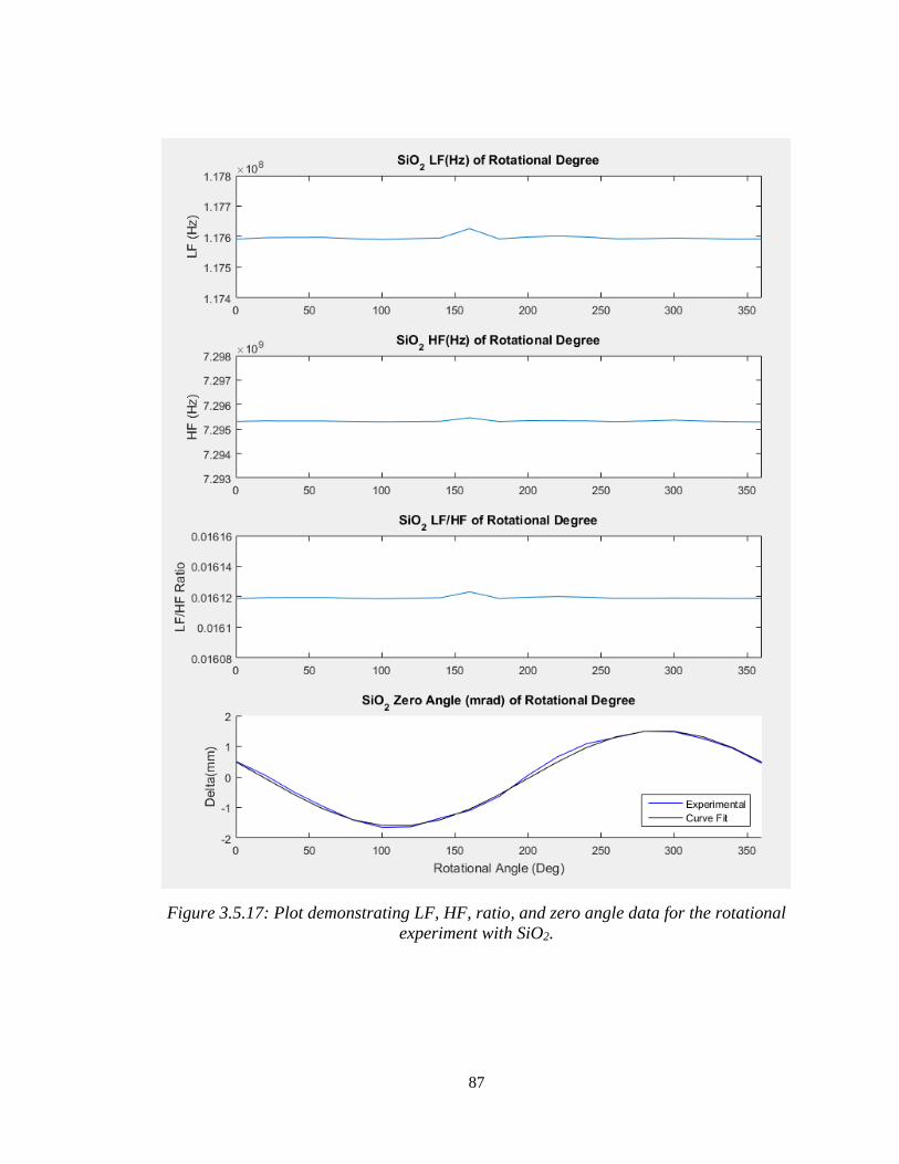
87
Figure 3.5.17: Plot demonstrating LF, HF, ratio, and zero angle data for the rotational
experiment with SiO2.

88
What was evident in this data was that while rotation greatly affected the position
of the zero angle, after correcting for the delta when setting the sample to the desired angle
(4 mrad pitch), there was a remarkable stability despite the rotation of the sample.
Additionally, when inserting the sample purposefully incorrect, the change in zero angle
witnessed was much more dramatic. In summary, it appears the observed effects did not
have to do with the parallel faces of the sample or the crystalline structure.
One final experiment was planned to monitor the zero angle change due to rotation,
however, this time the placement of the sample in the mount would be intentionally altered.
The thought at this point was that what was being seen was in fact due to the extreme
unlikelihood of placing the sample perfectly into the mount. The set screw that holds the
sample in place does not press down on the center of the cylindrical sample and thus,
depending on tightness, would cause some initial change in set position which would most
likely cause the sinusoidal change in zero angle being witnessed. The Figure 3.5.18 below
illustrates the set screw issue as described with an exaggerated tilt (pitch) angle.
Figure 3.5.18: Simple depiction of the FPE mount, (a) demonstrates the perfect
placement of an FPE, (b) demonstrates the potential effect of tightening the set
screw that can change the zero angle. The crystal is oriented in this figure so the
laser path is left and right.
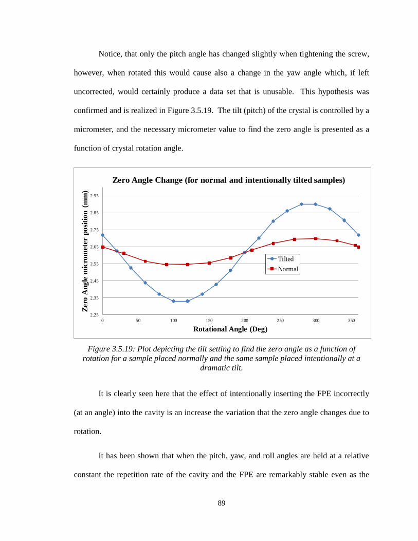
89
Notice, that only the pitch angle has changed slightly when tightening the screw,
however, when rotated this would cause also a change in the yaw angle which, if left
uncorrected, would certainly produce a data set that is unusable. This hypothesis was
confirmed and is realized in Figure 3.5.19. The tilt (pitch) of the crystal is controlled by a
micrometer, and the necessary micrometer value to find the zero angle is presented as a
function of crystal rotation angle.
Figure 3.5.19: Plot depicting the tilt setting to find the zero angle as a function of
rotation for a sample placed normally and the same sample placed intentionally at a
dramatic tilt.
It is clearly seen here that the effect of intentionally inserting the FPE incorrectly
(at an angle) into the cavity is an increase the variation that the zero angle changes due to
rotation.
It has been shown that when the pitch, yaw, and roll angles are held at a relative
constant the repetition rate of the cavity and the FPE are remarkably stable even as the
2.25
2.35
2.45
2.55
2.65
2.75
2.85
2.95
0 50 100 150 200 250 300 350
Zero
An
gle
mic
rom
ete
r p
osi
tio
n (
mm
)
Rotational Angle (Deg)
Zero Angle Change (for normal and intentionally tilted samples)
Tilted
Normal

90
rotation is changed. This relaxes the requirement of always placing the sample at the same
rotational angle for each scan while ensuring that the data produced will be usable and
reliable. Additionally, this effect can be used in future research to determine how well an
FPE has been placed into a cavity, a method that could be useful in many laser physics
applications.
3.6 Control Samples and Daily Variation
While, the data from these repeatability and characterization experiments suggests
very stable and precise data, it became apparent that over a period of weeks there seemed
to be some drift back and forth in the data. Specifically, the frequency ratio would fluctuate
to a greater degree than observed in the repeatability analysis. This is shown for the two
control samples, A15-1 and A15-2, over a period of measurements spanning two weeks.
Figure 3.6.1: Demonstration of the change in the frequency ratio for sample A15-1 over
a period of two weeks. The standard deviaiton of the entire population was 1.37x10⁻⁶

91
Figure 3.6.2: Demonstration of the change in the frequency ratio for sample A15-2 over
a period of two weeks. The standard deviaiton of the entire population was 1.536x10⁻⁶
This data demonstrates the daily variation as measured in the two control samples
and contrary to the stability in the single day repeatability experiments it seems that over a
longer period of time the data drifts back and forth. After close examination, it was
determined when considering the laboratory environment that one of the factors in this
change is a correlation between the frequency ratio and the humidity and pressure within
the lab. A closer examination of this is provided in Section 5.2 and an analysis of the data
trends with the laboratory environment is provided in Appendix B. A correction was
generated utilizing control samples and this was done for all the data produced in the latter
portion of this work. The measured LF/HF ratio of a test sample can be compared with the
LF/HF ratio of control samples to correct for environmental changes. By tracking the daily
change in the control samples a simple arithmetic correction is applied to the irradiated
sample data to extract the measured refractive index change. This correction was
completed by measuring the control samples and the irradiated samples on the same day

92
with similar laboratory environments. By doing this both before and after a sample was
irradiated, the baseline measured for the irradiated sample could be adjusted based on the
daily variation in the control samples in order to update the irradiated baseline to a value
that is representative of what it would have been, had it been measured on the same day
with the same laboratory environment as the post-irradiation measurement.
3.7 Calibration and Repeatability Conclusions
There were several things to take away from these repeatability analysis experiments.
The first is the vast superiority of performing a cavity length scan instead of an angle scan.
The measurement stability of the cavity length scan leads to a standard deviation nearly
100 times better than that of the angle scans. These values also take into account the
repeatability of placement since between each trial the sample was removed and placed
back into the mount by hand. In addition, the ability to largely ignore crystal rotation when
removing and inserting the FPE into the cavity, provided that the other angles remain
consistent, is very useful. The only repeatability issue that remains is that over a period of
days the frequency ratio as measured tends to drift, even with no intentional system
changes. This can be due to any number of factors in the laser cavity including the
laboratory environment and the functioning of the laser itself. One of the largest battles to
be fought daily is dust. Dust accumulating on the mirrors, lenses, and prisms in the cavity
has a dramatic effect on not only the data stability but also the overall ability to mode-lock
the laser. However, as mentioned, this daily variation is corrected for by measuring control
samples along with the irradiated sample in order to adjust the baseline measurement for
their radiated sample enabling the necessary comparison for refractive index change.

93
Chapter 4: Irradiation Methodology
4.1 Crystal Irradiation Methodology
The next stage of this research included the irradiation of physical CaF2 crystal
samples. This was accomplished utilizing three experimental apparatuses. The first
utilized a Nuclear Chicago (NH-3) Neutron Howitzer containing a 6 Curie (Ci) PuBe
neutron source. The second used the 350-keV Cockroft-Walton accelerator at Sandia
National Laboratory’s Ion Beam facility, which was calibrated to produce a D-D
(Deuterium-Deuterium) and D-T (Deuterium-Tritium) fusion neutron yield. The third and
final set of experiments was performed using the Oregon State University TRIGA reactor.
The primary purpose of these irradiation experiments was intended to demonstrate
measurements of neutron induced refractive index change and a beginning calibration to
allow for assessment of unknown neutron fields in the future using these refractive index
measurement techniques. This will ultimately allow for the ground work in applying this
work towards its goal of high precision dosimetry. Each sample’s thickness and diameter
was measured mechanically with a micrometer having the accuracy of 1/10 of 1/1000 of
an inch. The latter translates to an accuracy of about 2.54 microns. This allowed for a
moderate check of the length change and thus the density change of the material being
irradiated. Table 4.1.1 shows the original measurement results for samples numbering
A15-1 to A15-10. However, only samples A15-3 through A15-6 were irradiated.

94
Table 4.1.1: Table showing the physical measurements
of the first set of CaF2 samples.
CaF2 Pre-Irradiation (03/28/2016)
d (mm) t (mm) volume (cc)
A15-1 25.273 15.189 7.620
A15-2 25.298 15.187 7.634
A15-3 25.306 15.189 7.640
A15-4 25.273 15.187 7.619
A15-5 25.284 15.187 7.625
A15-6 25.273 15.184 7.617
A15-7 25.281 15.184 7.622
Table 4.1.2 shows the dimensions of samples B15-1 through B15-5 as measured on
January 24, 2017. Samples B15-1 and B15-2 were used as controls for the OSU irradiation
experiment while B15-3 through B15-5 were irradiated by OSU.
Table 4.1.2: Table showing the physical measurements
of the second set of CaF2 samples.
CaF2 Pre-Irradiation (01/24/2017)
d (mm) t (mm) volume (cc)
B15-1 19.981 14.975 4.696
B15-2 19.975 14.970 4.691
B15-3 19.975 14.970 4.691
B15-4 19.972 14.972 4.690
B15-5 19.980 14.971 4.694
4.1.1 NH-3 Neutron Howitzer Irradiation
The first irradiation apparatus was the NH-3 neutron howitzer. Within this apparatus
three experiments were completed with the intention to serve as a basic proof-of-principle
in an extremely low neutron flux environment that was easily accessible at UNM. These
three experiments included a 24 hour one time irradiation, a sequential irradiation from

95
zero to 221 days, and one final sequential irradiation from zero to 6.5 days. Several factors
that must be kept in mind during this research is not only the cumulative radiation absorbed
in a sample but also the average energy of the neutrons interacting with the material and
the flux of the neutrons (i.e., what is the rate at which neutrons are interacting with the
material). The average energy of the neutrons generated from the PuBe source in the
howitzer is about 5 MeV but they have a broad spectrum. An evaluation of the possible
neutron spectrum from the PuBe source is presented in Section 4.2.1. A representative
image of a commercial NH-3 Neutron Howitzer is included as Figure 4.1.1. The sample
to be irradiated is placed inside one of the two ports depicted half way down the
circumference of the cylindrical housing.
Figure 4.1.1: Photo of the NH-3 Neutron Howitzer by Nuclear Chicago

96
4.1.2 Sandia National Labs Irradiation
The second irradiation apparatus utilized a facility at Sandia National Laboratory to
generate to yield Deuterium-Deuterium (DD) and Deuterium-Tritium (DT) fusion
neutrons. The experiment was completed in two stages. The first was a campaign of
irradiations that yielded in an absorbed dose of 3.15 Gy after which refractive index
measurements were performed. The second stage was an additional irradiation of the same
CaF2 sample adding an absorbed dose of 1.56 Gy which brought the total absorbed dose in
the sample to 4.71 Gy. This experiment was intended to provide another proof-of-principle
test to determine the long-term damage of the CaF2 sample exposed to a higher neutron
flux environment at two different neutron energies. The neutrons generated in this
irradiation experiment were generated with the 350-keV Crockroft-Walton accelerator at
Sandia National Laboratory’s Ion Beam facility by accelerating deuterium ions into either
an ErD2 or ErT2 targets to yield D-D and D-T fusion neutrons, respectively [57]. For this
work, the sample was located at 0 degrees relative to the beam which yielded mono-
energetic neutrons having energies of 2.91 MeV and 14.79 MeV for the D-D and D-T
reactions, respectively. The fluence for the CaF2 sample was determined by Sandia
National Laboratory utilizing the Associated Particle Method [58]. The sample
experimental schematic of the setup utilized to generate D-T neutrons is shown in Figure
4.1.2.

97
Figure 4.1.2: Example schematic of experimental setup for
generating D-T neutrons at Sandia National Laboratory
4.1.3 Oregon State University Irradiation
The third irradiation apparatus utilized the outer ring of OSU’s TRIGA reactor. It
was primarily intended to produce an much greater fluence of incident neutrons on the
CaF2 samples than was able to be performed by the NH-3 Howitzer or the Sandia apparatus.
These three samples were subjected to a fast and near-fast neutron (100 keV – 10 MeV)
flux of 2.51x10¹³±4.75x10¹² n/cm2s, sufficient to cause numerous, high energy PKAs in
CaF2. Three samples were irradiated at varied lengths of time in order to achieve a neutron
fluence of 1.70x10¹⁶, 1.70x10¹⁷, and 1.70x10¹⁸ neutrons/cm2 for samples B15-4, B15-5,
and B15-3, respectively.
4.2 Estimating Radiation Fluence, Energy Fluence, and Dose with MCNP
In order for accurate data tracking and ultimately correlation with refractive index
change an accurate estimation of fluence, energy fluence and absorbed dose must be
determined. For the first irradiation experiment, using the NH-3 neutron Howitzer, the
fluence, energy fluence, and dose was calculated using an MCNP code designed to model

98
the neutron Howitzer. Utilizing an f4 tally the flux in the sample will be calculated and
using an f6 tally the rate of energy deposited in the sample the dose rate can be estimated.
This option in MCNP generates a value of rate of energy deposited with the units of
𝑀𝑒𝑉/(𝑔 ∗ 𝑠). This leaves only a simple conversion to get the value into a desirable form.
Due to the complications of modeling the Sandia National Labs irradiation setup the
fluence was determined by staff performing the experiments. However, given the fairly
monoenergetic nature of the D-D and D-T neutrons delivered, the calculation of energy
fluence and dose is a simple conversion using MCNP output. Similarly, energy fluence and
dose data for the OSU irradiation experiments was obtained in the same fashion using
MCNP as a guide.
4.2.1 NH-3 Neutron Howitzer MCNP Modeling
The first step is to estimate the dose received in the irradiated CaF2 in the NH-3. A
full model of the NH3 Neutron Howitzer, developed by Steve Su, was modified to
incorporate a CaF2 and the neutron flux profile and dose rate profile were determined using
an F6 tally in MCNP. A crucial piece of this puzzle is the definition of the source spectrum.
The source in the NH-3 Neutron Howizer is a Plutonium-Beryllium (PuBe) source, with
neutrons from the Be(a,n) reaction and directly from Pu fission. Source spectra has been
derived for various PuBe sources with varying Pu content [59]. For this research the Pu
content in the PuBe source was assumed to be 83%. It is worth noting that the difference
in the source spectrum for 77%, 83% and 95% are minimal as shown in Figure 4.2.1. The

99
average neutron energy from the 83% Pu content PuBe source was calculated to be
approximately 5.09 MeV.
Figure 4.2.1: Source Spectrum for in a PuBe source with varying Pu content [59].
The MCNP code was modified to use the spectrum shown in Figure 4.2.1 to
represent the NH-3 system, to more accurately estimate the flux and the dose in a CaF2
sample. The geometry of the NH-3 Neutron Howitzer built within MCNP is shown in
Figure 4.2.2 observing the XY plane and in Figure 4.2.3 observing the XZ plan. The
number designations in the figures correspond to layers as follows:
1. Paraffin
2. Aluminium
3. Air
4. PuBe source

100
5. Aluminum
6. Air
7. Aluminum
8. Lucite
9. Calcium Fluoride (CaF2)
10. Air
Figure 4.2.2: XY-plane view of the MCNP geometries for the NH-3
Neutron Howizer with 15 mm CaF2 sample inserted (as region 9).

101
Figure 4.2.3: XZ-plane view of the MCNP geometries for the NH-3
Neutron Howizer with 15 mm CaF2 sample inserted (as region 9).
Using an F4 and F6 tally the average neutron flux and energy deposition can be
calculated inside a specified region. Setting that region to surface 9 as shown in Figure
4.2.2 and Figure 4.2.3 allows for the calculation inside the CaF2 sample. MCNP uses
energy bins to calculate flux and energy distribution. The flux per energy bin for the 6.5
mm and 15 mm thick CaF2 samples is shown in Figure 4.2.4. Both thicknesses were
considered for measurements, though only 15 mm samples were eventually used. This
figure shows the distribution by energy of the flux in the CaF2. By adding the energy bins
together one can get a value for the total flux. Because MCNP normalizes the flux and
energy distribution to a single neutron. In order to get the actual flux, the output from
MCNP must be multiplied by the source strength. The source strength due to lack of
documentation on the utilized source was determined by published data for PuBe sources

102
and is given to be approximately 1.2x10⁷ n/s [60]. This gives the results for flux in the
CaF2, presented per energy bin in Figure 4.2.4.
Figure 4.2.4: MCNP calculated flux distribution in CaF2 samples.
From these flux quantities, the energy flux can be calculated using Equation 28.
𝜓 = 𝜑𝐸𝑏𝑖𝑛 (Eq. 28)
where 𝜓 is the energy flux and φ is the neutron flux. Using an F4 and F6 tally the average
neutron flux and energy deposition can be calculated inside a sample further leading to the
dose estimation. Figure 4.3.6 shows the energy flux as a function of Energy. Again,
creating a sum of all of the energy bins will give a value for total Energy Flux.
0.00E+00
1.00E+03
2.00E+03
3.00E+03
4.00E+03
5.00E+03
6.00E+03
Neu
tro
n F
lux (
n/c
m2*s)
Energy Bin (MeV)
Flux per Energy Bin (from MCNP calculation)
15mm CaF2 Sample
6.5mm CaF2 Sample
Total Flux (15mm):6.55E4 n/cm2*s
Total Flux (6.5mm):7.29E4 n/cm2*s

103
From this quantity, a simple calculation of dose can be obtained using the neutron
kerma factor and making the assumption that the chamber is in charged particle equilibrium
[61]. Due to the largely homogenous interaction of the neutrons within the crystal and the
minimal range of the PKAs (i.e., charged particles) this approximation is acceptable. The
only place this would not be a solid approximation is at the surface of the crystal were some
atoms are not moving or may leave the crystal if they are struck by highly energetic
neutron. The dose, D, can be determined from the kerma factor, K, which is
𝐷 = 𝐾 = 𝛷𝐹𝑛 (Eq. 29)
for a monoenergetic neutron fluence with the neutron kerma factor, 𝐹𝑛, for that energy.
The kerma depends on the energy transferred to charged particles, and dose depends on
energy absorbed, but these are close and the two quantities are treated as such. The neutron
kerma factor 𝐹𝑛 can be obtained from literature for a variety of materials and neutron
energies [62]. For the 15 mm thick CaF2 crystal sample, assuming an average neutron
energy of 5 MeV and using the previously determined flux spectrum in Figure 4.2.4, the
total energy flux is 1.88 x10⁵ MeV·n/cm2·s. The neutron kerma factor for 5 MeV neutrons
is 6.62x10⁻¹⁰ rad·cm2 [62]. Using this value and the energy flux, a dose rate of 3.86x10⁻⁵
rad/s or 3.86x10⁻⁷ Gy/s. Thus, the total dose over a 24 hr period would be 0.0159 Gy for
the 15 mm thick sample. Due the slightly higher flux in the 6.5 mm sample the estimated
dose rate is also slightly higher and comes out to 0.0208 Gy. These accuracy of these
calculations is increased by discretizing the flux into bins that fit a defined kerma factor.
At this point, these calculations can be compared side by side with discretized
calculations of dose utilizing the flux-to-dose conversion factors, which is a commonly

104
utilized way of estimating dose, quoted by NCRP-38 and ANSI/ANS-6.1.1-1977. These
flux-to-dose conversion factors and associated Q-values are shown in Table 4.2.1.
Table 4.2.1: Values of Dose Factor and
Quality Factor for converting flux-to-dose
per NCRP-38 and ANSI/ANS-6.1.1-1977.
Energy
(MeV)
Dose Factor
(rem/hr)/(n/cm2·s)
Quality
Factor
0.001 3.76 x10⁻⁶ 2.0
0.01 3.56 x10⁻⁶ 2.5
0.1 2.17 x10⁻⁵ 7.5
0.5 9.26 x10⁻⁵ 11.0
1.0 1.32 x10⁻⁴ 11.0
2.0 1.25 x10⁻⁴ 9.0
2.5 1.25 x10⁻⁴ 9
5.0 1.56 x10⁻⁴ 8.0
7.0 1.47 x10⁻⁴ 7.0
10.0 1.47 x10⁻⁴ 6.5
14.0 2.08 x10⁻⁴ 7.5
Using these values and the flux bins from Figure 4.2.4 an estimation of dose can be
created tracking the dose based on the number of days the sample remains in the NH-3
neutron howitzer. This is done through fitting the discretized energy bins into a dose factor
bin. Due to the nature of the typical application (biological dose equivalent) of this table
the values are quoted in rem/hr. However, because this work is only concerned with
absorbed dose a simple conversion utilizing the Q-factor is performed. The Q-, or Quality
Factor, is a conversion factor between absorbed dose and equivalent dose. Since, absorbed
dose is the standard quantity for this work the Q factor was divided out to obtain the final
absorbed dose estimation. From this point the flux is multiplied by the dose factor giving
a dose rate in rad/hr. This can further be adjusted to units of Gy/hr simply by dividing by

105
100 since 1 Gy = 100 rad. A comparison of calculated absorbed dose in a 15 mm thick
cylindrical sample of CaF2 is demonstrated in Table 4.2.2. The comparison is between
dose as calculated using neutron kerma factors and dose calculated using flux-to-dose
conversion factors from NCRP-38 and ANSI/ANS-6.1.1-1977.
Table 4.2.2: Comparison of Dose values calculated by kerma
factor and by dose factor using a discretized sampling of the
flux spectrum as generated by the MCNP code.
Days in NH-3
Howitzer
Dose (Gy) from
Kerma Factor
Dose (Gy) from
Dose Factor
0 0.00 0.00
7 0.111 1.38
22 0.350 4.35
41 0.653 8.10
56 0.891 11.07
85 1.353 16.80
98 1.559 19.37
144 2.292 28.46
221 3.517 43.67
It was clear at this point that there was something amiss in the comparison of these
calculations. Upon further examination, it was discovered that the flux-to-dose conversion
factors in the MCNP manual are based on the kerma factors for human tissue as their
primary application is for biological equivalent dose. Because, this work is focused on
CaF2, and the kerma factors for CaF2 are quite different than that of human tissue, kerma
factors were used to obtain dose values for this work. Please note that the utilization of
kerma factors to estimate dose is accurate for charged particle equilibrium (CPE)
environments which is a reasonable assumption for our samples. CPE for the recoil atoms
is established very close to the crystal face so, except for a thin region near the crystal

106
faces, CPE is a reasonable estimation. A full list of these kerma factors is included in Table
4.2.3.
Table 4.2.3: Kerma Factors for CaF2 as quoted from Caswell [62].
Energy
(MeV)
Kerma
Factor
(rad∙cm2)
Energy
(MeV)
Kerma
Factor
(rad∙cm2)
Energy
(MeV)
Kerma
Factor
(rad∙cm2)
0.002 7.36x10⁻¹³ 1.25 1.08x10⁻¹⁰ 6.00 8.45x10⁻¹⁰
0.004 8.91x10⁻¹³ 1.50 1.06x10⁻¹⁰ 6.20 8.54x10⁻¹⁰
0.006 1.15x10⁻¹² 1.75 1.23x10⁻¹⁰ 6.60 8.83x10⁻¹⁰
0.011 1.60x10⁻¹² 1.95 1.44x10⁻¹⁰ 7.00 9.53x10⁻¹⁰
0.020 2.49x10⁻¹² 2.30 1.66x10⁻¹⁰ 7.40 9.95x10⁻¹⁰
0.036 6.07x10⁻¹² 2.50 2.15x10⁻¹⁰ 7.80 1.02x10⁻⁹
0.063 1.06x10⁻¹¹ 2.70 2.39x10⁻¹⁰ 8.00 1.05x10⁻⁹
0.082 1.03x10⁻¹¹ 3.10 2.99x10⁻¹⁰ 8.20 1.07x10⁻⁹
0.086 1.49x10⁻¹¹ 3.30 3.29x10⁻¹⁰ 8.60 1.13x10⁻⁹
0.090 2.25x10⁻¹¹ 3.50 3.75x10⁻¹⁰ 9.00 1.16x10⁻⁹
0.094 3.67x10⁻¹¹ 3.70 4.14x10⁻¹⁰ 9.40 1.21x10⁻⁹
0.098 5.34x10⁻¹¹ 3.90 4.54x10⁻¹⁰ 9.80 1.27x10⁻⁹
0.105 3.85x10⁻¹¹ 4.20 5.35x10⁻¹⁰ 10.50 1.38x10⁻⁹
0.250 4.19x10⁻¹¹ 4.60 6.21x10⁻¹⁰ 11.50 1.56x10⁻⁹
0.500 5.71x10⁻¹¹ 5.00 6.62x10⁻¹⁰ 12.50 1.72x10⁻⁹
0.740 5.97x10⁻¹¹ 5.40 7.46x10⁻¹⁰ 14.50 1.88x10⁻⁹
1.05 7.69x10⁻¹¹ 5.80 8.35x10⁻¹⁰ 15.5 1.96x10⁻⁹
From these kerma factors a dose chart can be developed to show the accumulated
dose in a sample placed in the NH-3 Howitzer over time. This dose chart is shown in
Figure 4.2.5 as the secondary axis while the primary axis shows the total neutron fluence
associated with a particular dose.
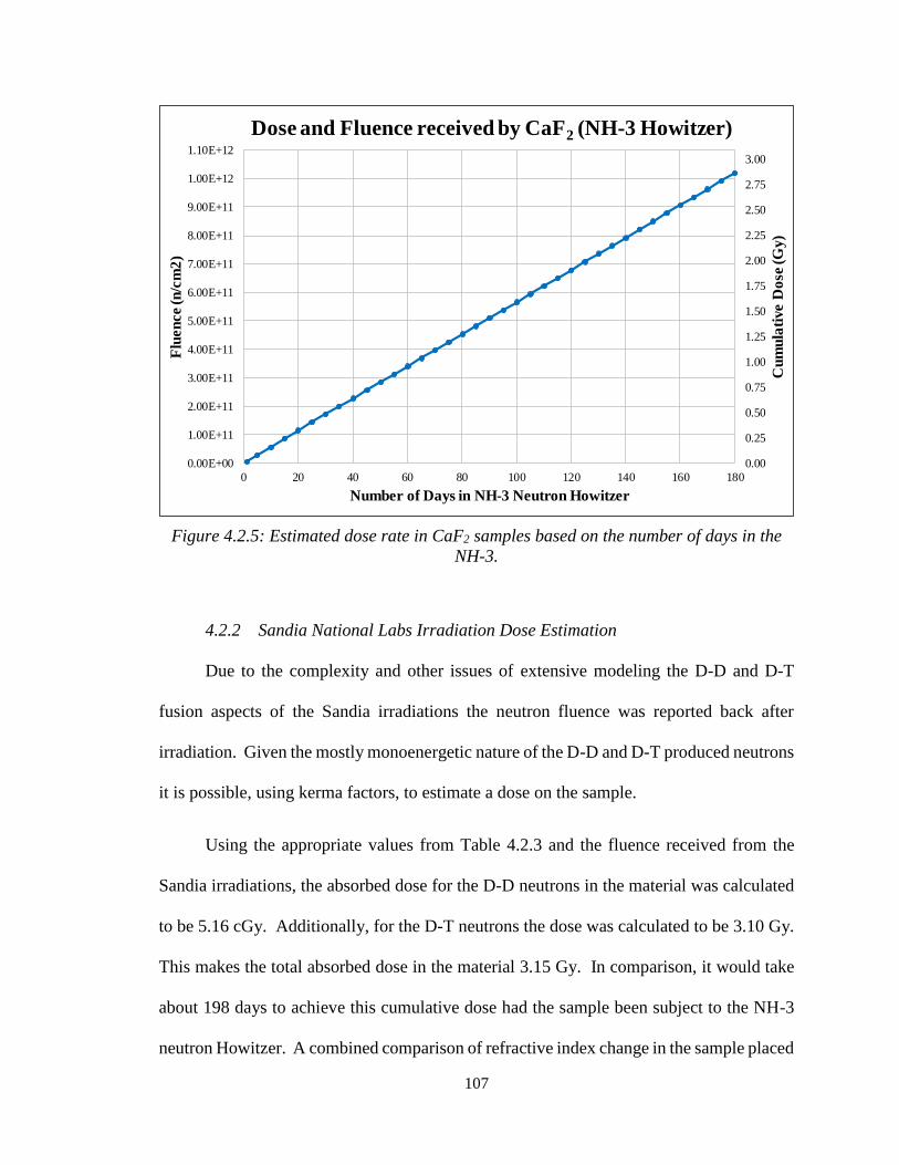
107
Figure 4.2.5: Estimated dose rate in CaF2 samples based on the number of days in the
NH-3.
4.2.2 Sandia National Labs Irradiation Dose Estimation
Due to the complexity and other issues of extensive modeling the D-D and D-T
fusion aspects of the Sandia irradiations the neutron fluence was reported back after
irradiation. Given the mostly monoenergetic nature of the D-D and D-T produced neutrons
it is possible, using kerma factors, to estimate a dose on the sample.
Using the appropriate values from Table 4.2.3 and the fluence received from the
Sandia irradiations, the absorbed dose for the D-D neutrons in the material was calculated
to be 5.16 cGy. Additionally, for the D-T neutrons the dose was calculated to be 3.10 Gy.
This makes the total absorbed dose in the material 3.15 Gy. In comparison, it would take
about 198 days to achieve this cumulative dose had the sample been subject to the NH-3
neutron Howitzer. A combined comparison of refractive index change in the sample placed
0.00
0.25
0.50
0.75
1.00
1.25
1.50
1.75
2.00
2.25
2.50
2.75
3.00
0.00E+00
1.00E+11
2.00E+11
3.00E+11
4.00E+11
5.00E+11
6.00E+11
7.00E+11
8.00E+11
9.00E+11
1.00E+12
1.10E+12
0 20 40 60 80 100 120 140 160 180
Cu
mu
lati
ve D
ose
(G
y)
Flu
en
ce (n
/cm
2)
Number of Days in NH-3 Neutron Howitzer
Dose and Fluence received by CaF2 (NH-3 Howitzer)

108
in the Howitzer and the sample irradiated at Sandia National Laboratories will be presented
in Section 5.7. As previously mentioned sample A15-5 was irradiated further at Sandia
National Labs such that upon the second refractive index measurement the total absorbed
dose was calculated to be 4.71 Gy.
4.2.3 Oregon State University Irradiation Dose Estimation
In a similar way to the Sandia irradiation experiments Oregon State University
provided some very helpful information towards calculating the fluence and dose received
in the irradiated samples. They have generated flux profiles for their TRIGA reactor
utilizing two primary calculation methods. The primary method is through MCNP similar
to what has been done in this research for the NH-3 neutron howitzer. Additionally, they
have utilized STAY-SL, a dosimetry unfolding application with activation, dosimetry, and
flux error calculation developed and maintained by the Nuclear Energy Agency (NEA).
The CaF2 crystals were placed in the G-Ring In-Core Irradiation Tube (GRICIT-C) region
of the TRIGA reactor. The results of the calculated flux profile in this region are plotted
in Figure 4.2.6.

109
Figure 4.2.6: Plot of the MCNP and STAY’SL flux profile in the GRICIT-C region of the
OSU TRIGA reactor. All doses in this work were calculated using the MCNP flux values.
Utilizing the data in Figure 4.2.6 a discretized calculation of dose can be performed
in a similar way for both the Howitzer and the Sandia irradiation experiments were
calculated. Utilizing the values already quoted in Table 4.2.3 and creating energy bins for
the flux values in Figure 4.2.6 dose values were generated for these irradiated samples. As
previously mentioned, sample B15-4 received a total neutron fluence of 1.70x10¹⁶ n/cm2,
sample B15-5 received a total neutron fluence of 1.70x10¹⁷ n/cm2, and sample B15-3
received a total neutron fluence of 1.70x10¹⁸ n/cm2. The dose calculated by this method
for each of these irradiations was 1.99x10⁴ Gy, 1.99x10⁵ Gy, and 1.99x10⁶ Gy (or 19.9
kGy, 199 kGy, and 1.99 MGy), respectively. By comparison, in order to achieve this dose
within the NH-3 Howitzer the sample would have to be irradiated for about 420 millennia.
5E+09
5E+10
5E+11
0.01 0.1 1 10
Flu
x (
n/c
m2
*s)
Energy (MeV)
Oregon State University GRICIT-C Fast Flux Profile
STAY'SL
MCNP

110
Chapter 5: CaF2 Irradiation Results and Analysis
5.1 Overview
The experimental thrust of this research is the ability to perform precise
measurements of the change of refractive index in a CaF2 crystal sample. An array of CaF2
samples were irradiated according to the plan laid out in Section 4.1. Table 5.1.1 shows
the range of neutron fluences, energy fluences, absorbed doses received by the various
CaF2 samples. Values separated by a dash (–) indicate that the sample was irradiated
continuously and measurements were taken at various points between the lower and upper
bounds indicated. Values separated by an ampersand (&) indicate that the sample was
irradiated a fixed number of times and measured at the values indicated.
Table 5.1.1: Master table showing the neutron fluence, energy fluence and absorbed dose
values associated with each irradiated CaF2 sample. Doses were calculated using MCNP
and provided fluence values for energies above 2 keV. Per Chapter 2, 2 keV is close to
the required neutron energy to create a PKA that will cause a damage cascade.
Master Table of CaF2 Irradiation Values Sample
ID
Irradiation
Source
Neutron Fluence
(n/cm2)
Energy Fluence
(MeV/cm2)
Absorbed Dose
(Gy)
A15-1 N/A N/A N/A N/A
A15-2 N/A N/A N/A N/A
A15-3 Howitzer 5.95x10⁹ 2.97x10¹⁰ 0.0159
A15-4 Howitzer 4.16x10¹⁰ – 1.31x10¹² 2.08x10¹¹ – 6.57x10¹² 0.11 – 3.52
A15-5 Sandia 1.85x10¹¹ & 2.68x10¹¹ 2.37x10¹² & 3.49x10¹² 3.15 & 4.71
A15-6 Howitzer 1.04x10¹⁰ – 3.88x10¹⁰ 5.20x10¹⁰ – 1.94x10¹¹ 0.028 – 0.104
B15-1 N/A N/A N/A N/A
B15-2 N/A N/A N/A N/A
B15-3 OSU 1.70x10¹⁶ 1.95x10¹⁶ 1.99x10⁴
B15-4 OSU 1.70x10¹⁷ 1.95x10¹⁷ 1.99x10⁵
B15-5 OSU 1.70x10¹⁸ 1.95x10¹⁸ 1.99x10⁶

111
Contain within this chapter are the results of the periodic measurements taken of each of
the samples mentioned in Table 5.1.1. All calculated doses only include incident neutrons
greater than or equal to 2 keV due to the required PKA energy for semi-permanent damage
as calculated in Chapter 2.
5.2 Obtaining Results
This section will serve to indicate the basic process for how results are obtained
combining all of the theory and practice discussed to this point. In order to obtain accurate
and consistent results despite some of the difficulties presented in this work the first step
was to establish two or more control samples that served to correct for variation due to
laboratory environment, cavity parameter drift, and other unquantified errors. Frequency
ratio measurements for the control samples were completed before and after every
irradiation experiment along with the measurement of the irradiated sample (or non-
irradiated sample in the case of the pre-irradiation baseline measurements). By utilizing
the frequency ratio results for the control samples, the correction described in Section 5.4
for the correction of the Howitzer data was utilized. This correction is added to the original
baseline measurement of the frequency ratio for the pre-irradiated sample, correcting the
baseline to appear as if it had been measured the same day as the post-irradiation
measurement. Then the division of the pre-irradiation frequency ratio by the corrected
post-irradiation measurement was completed, per Equation 30 (also shown previously as
Equation 25), where the subscript 0 represents the pre-irradiation values and the subscript
1 represents the post-irradiation values, to find a super ratio.
ℝ =ℛ0
ℛ1=
𝑛𝑝,𝑓𝑝,1
𝑛𝑝,𝑓𝑝,0=
𝑛𝑝,𝑓𝑝,0+Δ𝑛𝑝,𝑓𝑝
𝑛𝑝,𝑓𝑝,0= 1 +
Δ𝑛𝑝,𝑓𝑝
𝑛𝑝,𝑓𝑝,0 (Eq. 30)

112
At this point, Equation 30 is solved for Δ𝑛𝑝,𝑓𝑝 to obtain the change in refractive index
of the crystal. After this a comparison of the super ratio of the control samples was
completed. The super ratio between control samples should not change. However, a
change was witnessed and therefore suggests some other unquantified variation in the
system. The variation in the super ratio value was applied to the uncertainty in the change
of refractive index for each measurement, thus obtaining the final reported results.
5.3 Correcting for Daily Variation in Frequency Ratios
As previously discussed, the primary forms of measurement that produce the data to
be analyzed come in the form of the repetition rate of the cavity in frequency units, 𝜈𝑟𝑡,
and the repetition rate of the FPE, 𝜈𝑓𝑝, in frequency units. Dividing 𝜈𝑟𝑡 by 𝜈𝑓𝑝 results in
the standard frequency ratio we used for analysis of the sample as demonstrated by Eq. 24.
This ratio is obtained for each measurement pre- and post-irradiation, for multiple samples.
Also, as mentioned in Section 3.6, a minimum of two control samples were also
measured on each day an irradiated sample was measured, allowing for a correction to be
made as to the daily variation in the frequency ratio. In the case of the NH-3 neutron
Howitzer irradiations, samples A15-1 and A15-2 were measured as control samples. and
Later, B15-1 and B15-2 were also added as control samples. Samples A15-3, A15-4, and
A15-6 were irradiated. During the course of this research it was clear that over a period of
days there were changes noticed in the frequency ratios between non-irradiated samples,
so these are important to correct for when analyzing irradiated samples. This is completed
in the way described in Section 3.6. These day to day changes result in a change in the
frequency ratio in controlled samples, shown in Figure 5.3.1.
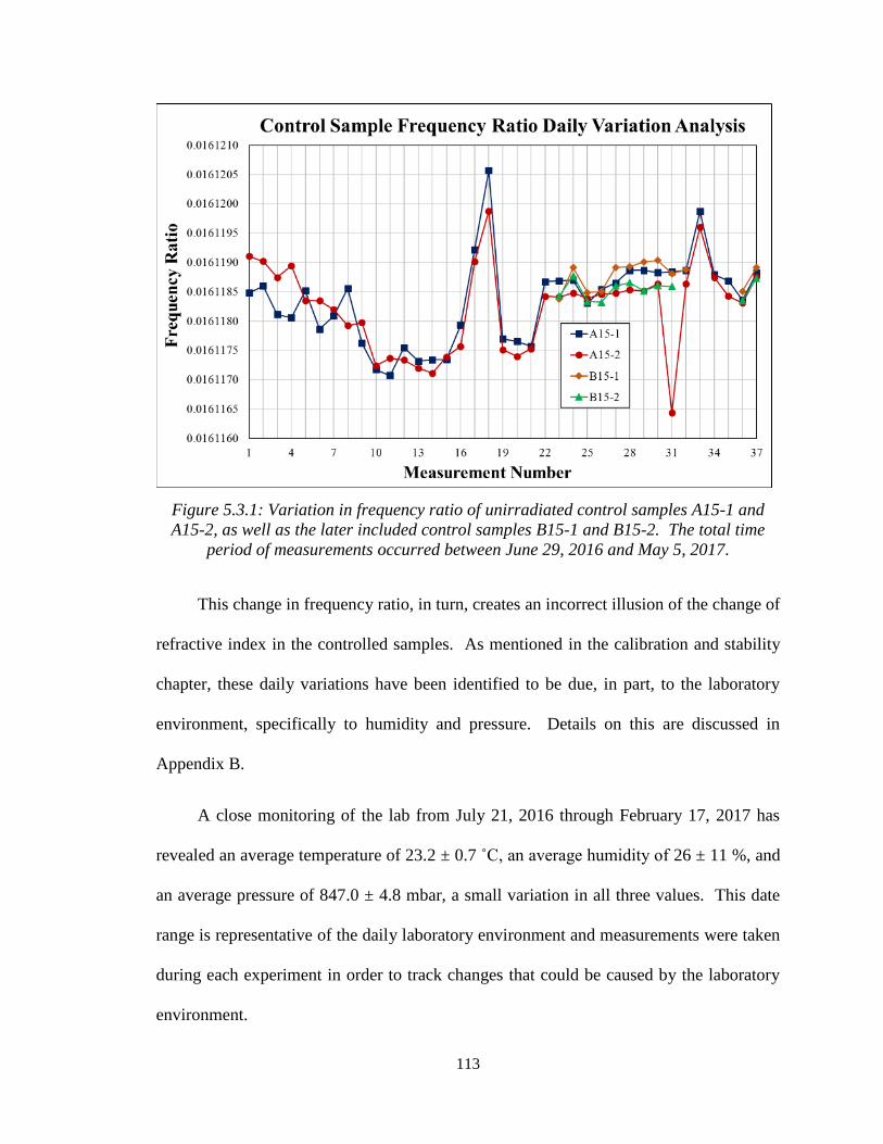
113
Figure 5.3.1: Variation in frequency ratio of unirradiated control samples A15-1 and
A15-2, as well as the later included control samples B15-1 and B15-2. The total time
period of measurements occurred between June 29, 2016 and May 5, 2017.
This change in frequency ratio, in turn, creates an incorrect illusion of the change of
refractive index in the controlled samples. As mentioned in the calibration and stability
chapter, these daily variations have been identified to be due, in part, to the laboratory
environment, specifically to humidity and pressure. Details on this are discussed in
Appendix B.
A close monitoring of the lab from July 21, 2016 through February 17, 2017 has
revealed an average temperature of 23.2 ± 0.7 ˚C, an average humidity of 26 ± 11 %, and
an average pressure of 847.0 ± 4.8 mbar, a small variation in all three values. This date
range is representative of the daily laboratory environment and measurements were taken
during each experiment in order to track changes that could be caused by the laboratory
environment.

114
Repeating this experiment under much more stable laboratory environments for four
control samples that were used for the OSU TRIGA irradiation data yielded a more stable
plot of the frequency ratio. It should be noted that the span of dates for these measurements
was only 4 days. This data also supports the expectation that this daily variation is largely
tied to laboratory environments since the laboratory environment was more stable for these
measurements. The environment averaged a temperature of 23.1 ± 0.5 ˚C, an average
humidity of 20 ± 2%, and an average pressure of 843.8 ± 4.4 mbar. A plot of the results
from this secondary test on non-irradiated control samples is shown in Figure 5.3.2. The
y-axis values are the same as in Figure 5.3.1 for comparison.
Figure 5.3.2: Secondary daily variation experiment with much better laboratory
environment stability.
The data in Figure 5.3.2 demonstrates a higher stability in the data. However, there
is still some notable deviation, particularly with sample A15-1. It should also be noted, for

115
future error analysis, that when considering the variation in these four data points of sample
A15-1, there is an “apparent” refractive index change averaging 9.62x10⁻⁶.
This daily variation phenomenon can be corrected for (with some uncertainty) by
determining the change in refractive index of the irradiated samples by utilizing the control
sample data. By obtaining the frequency ratio for the control samples on the same days as
the irradiated samples are measured, it is possible to create a correction for the irradiated
data utilizing the data obtained for the control samples. Without this correction, due the
precise nature of the changes being measured, the data would appear to be random
following the pattern created by the drift of the laser cavity on a given day which can be
minutely effected by temperature and humidity as well as more noticeably effected by dust
and changes in the cavity required to maintain mode-locking. Changes in the cavity due
to the current setup are necessary and inevitable and on occasion, they too can be corrected
for utilizing a correction algorithm based on this data. An ancillary examination of
potential reasons for the cause of these daily changes was completed. This examination is
included as Appendix B.
In order for a data correction to be made, the difference between the daily
measurement and the original day measurement is acquired and subtracted from the
measurement of the irradiated sample for that day. This is demonstrated by the correction
algorithm in Equation 31.
ℛ𝐶𝑜𝑟𝑟𝑒𝑐𝑡𝑦𝑒𝑑,𝑛 = ℛ𝑅𝑎𝑤,𝑛 − ∆ℛ𝐶,𝑛 (Eq. 31)
𝑤ℎ𝑒𝑟𝑒 ∆ℛ𝐶,𝑛 = {ℛ𝑐,𝑛 − ℛ𝑐,0}
116
In these equations 𝑅0 is the original baseline measurement for the controlled sample.
𝑅𝐶,𝑛 designates the frequency ratio of the control sample on day n and ∆𝑅𝐶,0 is the original
baseline measurement for the control. ∆𝑅𝐶,𝑛 is the daily correction that is calculated using
the change in the frequency ratio of the control sample between day n and the original
baseline. 𝑅𝑟𝑎𝑤,𝑛 is the ratio of the test crystal for day n. By subtracting the daily correction
from the raw ratio result of the irradiated sample a corrected value is generated which can
then be combined with the original baseline of the irradiated sample to produce the super-
ratio and then the change in refractive index. In the event of multiple control samples ∆𝑅𝐶
is calculated multiple times and the results are averaged before being added to ℛ𝑅𝑎𝑤,𝑛 to
extract the corrected ratio for the test crystal, ℛ𝐶𝑜𝑟𝑟𝑒𝑐𝑡𝑒𝑑,𝑛. After the baseline ratio is
corrected for the irradiated sample the change in refractive index can be calculated by
utilizing Equation 25 and Equation 26 from Section 3.3.4.
Given that the correction is necessary it is also necessary to apply some uncertainty
to the stated correction. This can be accomplished by utilizing the scatter of the super-ratio
of the control samples. Ideally, the super-ratio of control samples should remain constant
when compared day to day. The daily variation is expected as previously discussed, but
for measurements on the same day, without major environmental changes between
measurements, should remain constant. By tracking the separation of the control samples,
as seen in Figure 5.3.1, and applying the super ratio an uncertainty value can be applied to
each corrected data point. The uncertainty, developed using the daily change in the super-
ratio, represented in refractive index change, is demonstrated in Figure 5.3.3.

117
Figure 5.3.3: Confidence error in measurement correction by measurement day to
be applied to the refractive index change calculated in the irradiated sample.
The uncertainty is ultimately determined by the standard deviation of data shown
in Figure 5.3.3. This value applied to all refractive index change calculations after this
point is 2.35x10⁻⁵ which for the remainder of this work will be simplified to 2.4 x10⁻⁵.
For early data, these uncertainty calculations were based on only two unirradiated
control samples. However, two additional control samples were added in for the later data,
after recognizing the relatively high uncertainty associated with each data point. Several
major cavity changes took place during the time frame this data was acquired and thus the
uncertainty due these major cavity changes affecting the cavity dispersion, which in turn
affects the group velocities and the group index of refraction, are included in this
uncertainty calculation. Thus, for this work, the uncertainty calculation is considered quite
-1.7E-04
-1.2E-04
-7.0E-05
-2.0E-05
3.0E-05
8.0E-05
1 4 7 10 13 16 19 22 25 28 31 34 37
np
Un
cert
ain
ty
Measurement Number
Control Sample Variation Represented as np Uncertainty
A15-1
A15-2
B15-1
B15-2
Standard Deviation:
2.349x10⁻⁵

118
robust. A further tightening of this uncertainty is desirable to lower dose applications but
is outside of the scope of this work.
5.4 NH-3 Neutron Howitzer Irradiation Experiments
The first neutron howitzer experiment was a single irradiation of sample A15-3.
The sample was placed inside the NH-3 Howitzer for 23 hours and 56 minutes for a dose
of 0.0159 Gy. The sample was measured on four separate occasions after irradiation the
average refractive index change measurement was -1.1x10⁻⁵ ± 0.5x10⁻⁵ (the uncertainty
being the standard deviation of the four measurements). However, when the uncertainty,
calculated above, is included the measured change in the refractive index falls within the
noise of the uncertainty.
In order to increase refractive index change above uncertainties longer irradiations
were planned for the NH-3 Howitzer. This primary Howitzer experiment ultimately
included an accumulated irradiation of 221 days equating to approximately 3.52 Gy in
sample A15-4. The correction was applied (as well as the uncertainty), using the two
control samples A15-1 and A15-2, to sample A15-4 after each removal from the NH-3
howitzer to be measured. After each measurement, the sample was placed back into the
howitzer for continued irradiation. The calculated change in refractive index in sample
A15-4 is shown in Figure 5.4.1, plotted against absorbed dose as calculated from the
NCRP-38 values quoted in the MCNP manual [63]. The uncertainty bars are representative
of the uncertainty calculated from and displayed in Figure 5.3.3.

119
Figure 5.4.1: Demonstration of the Change in Refractive Index in CaF2 sample A15-4
which was exposed to PuBe Source Neutron Irradiation in the NH-3 Neutron Howitzer
for 221 days.
Figure 5.4.1 presents an inconclusive data set that seems to suggest that no
refractive index change is being measured or the change that is occurring is smaller the
uncertainty associated with the current measurement scheme. The modeling and
simulation portion of this work suggests that radiation damage is a largely cumulative
effect and thus the measured change is expected to consistently change over absorbed dose.
Because of the witnessed jumps in data one final howitzer irradiation was completed to
ensure that this data variation is due to the data uncertainty rather than a refractive index
change. This was completed with sample A15-6 to add additional data points between zero
days and seven days. The data produced is shown in Figure 5.4.2.
-1.0E-04
-8.0E-05
-6.0E-05
-4.0E-05
-2.0E-05
0.0E+00
2.0E-05
4.0E-05
6.0E-05
-0.5 0 0.5 1 1.5 2 2.5 3 3.5 4
Ref
ract
ive I
nd
ex C
ha
ng
e (Δ
n)
Absorbed Dose (Gy)
Refractive Index Change in Irradiated CaF2

120
Figure 5.4.2: Final Neutron Howitzer irradiation with sample A15-6 irradiated from 0 to
7 days.
Figure 5.4.2 demonstrates that, while the changes are not quite as dramatic as those
witnessed with the A15-4 irradiation, the jumps in the data points are consistently within
the overall uncertainty and any witnessed refractive index change is lost within the
uncertainty.
5.5 Sandia National Laboratories D-D and D-T Irradiation Experiment
The next result to consider was the irradiated sample (A15-5) exposed to Deuterium-
Deuterium and Deuterium-Tritium fusion produced neutrons. This sample was exposed to
a fluence of 2.35x10¹⁰ D-D neutrons/cm2, at 2.91 MeV, and 1.55x10¹¹ D-T neutrons/cm2,
at 14.79 MeV. Again, utilizing the flux-to-dose conversion factors the absorbed dose
received in this sample was 3.15 Gy. Figure 5.5.1 demonstrates the measured refractive
index change and shows all of the accumulated data measured for the Sandia irradiated
-5.0E-05
-4.0E-05
-3.0E-05
-2.0E-05
-1.0E-05
0.0E+00
1.0E-05
2.0E-05
3.0E-05
4.0E-05
-0.02 0 0.02 0.04 0.06 0.08 0.1 0.12
Ref
ract
ive I
nd
ex C
ha
ng
e (Δ
n)
Absorbed Dose (Gy)
Refractive Index Change in Irradiated CaF2

121
CaF2 samples (A15-5) including three baseline measurements and eight post-irradiation
measurements.
Figure 5.5.1: Demonstration of the full data set for the Sandia irradiated sample (A15-5)
measured on eight separate occasions post irradiation and three separate pre-irradiation
measurements.
The irradiated sample and the controls were measured eight times post-irradiation.
Utilizing a correction accounting for the daily change in frequency ratio a change in
refractive index averaging -6.4x10⁻⁵ ± 1.1x10⁻⁵ was measured. Recalling that each
measurement contains a set of at least 200 data points this change can also be represented
by the individual data points.
While, there is a distinction between the baseline and the irradiated data points, it
is also clear that there is a decent amount of variation in the data points even after applying
the corrections. In Figure 5.5.1, measurements from different days are represented by the
different colors, “irradiated 1” is a different day from “irradiated 2” and so on. There is an

122
obviouse variation between the average RI measurements day by day, as represented
previously in Figure 5.3.1. The level of variation must be considered in relation to the fact
that the change in refractive index is so small for this particular sample. If this is the
average amount of variation when measuring future samples that have received a higher
dose of radiation, the variation will be much less significant. To visualize this Figure 5.5.2
displays the point by point mean of the measurements with their associated standard
deviations. This plot gives a clearer example of the witnessed refractive index change in
the FPE.
Figure 5.5.2: Mean values for the baseline and irradiated measurents for the Initial
Sandia irraidated sample having recieved 3.15 Gy in absorbed dose.
As mentioned previously three measurements were utilized for the the pre-irradiation
measurement of sample A15-4. The average of these three trials necessarily became the
reference zero refractive index change point because the preirradiated sample had no
change in and of itself. After the pre-irradiation measurement was corrected for daily

123
variation utilizing the control samples A15-1 and A15-2. Within Figure 5.5.2 a single
measurement of the pre-irradiated baseline is shown to demonstrate the variation in the
baseline trials, while the post-irradiation measurement is a point-by point average of the
eight separate post-irradiation measurements. Thus, the refractive index change value at
each cavity length position is shown, relative to this zero. Additionally, there appears to
be an exaggerated decline in the post irradiation measurement with increased cavity length
with a greater negative slope than the baseline data. This particular phenomena is not
completely understood, although it can also be stated that when comparing single cavity
length scans that the slope of the ratio changes from time-to-time. A couple of factors that
could play into this variation are the relative straight placement of the translation stage that
the cavity end mirror is placed. Thus, if the end stage is not perfectly perpendicular to the
beam path it could present drift similar to this.
It certainly appears here that there was a measured refractive index change however
when again considering the uncertainty determined from Figure 5.3.3 rather than just the
standard deviation of the data the plot becomes a change is a bit more ambiguous as shown
in Figure 5.5.3. However, there still seems to be a clear change in refractive index for the
first of the two Sandia irradiations.

124
Figure 5.5.3: Initial Sandia irradiation results including overall uncertainty.
These results become much more ambiguous after the additional Sandia irradiation
occurred. The additional irradiation added about 1.56 Gy of total absorbed dose in the
sample. This brought the total absorbed dose to 4.71 Gy. The expectation given the
previous irradiation data and the results from the modeling and simulation portion of this
work was that the refractive index would decrease with more accumulated dose. However,
the measured refractive index change in sample A15-5 after the second irradiation changed
in the opposite direction of the expectation. Although, because of the uncertainty in the
data this change is still within the expected error and perhaps what was measured with after
the first Sandia irradiation was in fact not due to the change in refractive index but rather
the daily variation in the data. The results of both irradiations of sample A15-5 are shown
in Figure 5.5.4 demonstrating the positive index change measured after an additional 1.56
Gy of absorbed dose in the sample. A measurement, that if true, goes against understanding
-1.2E-04
-1.0E-04
-8.0E-05
-6.0E-05
-4.0E-05
-2.0E-05
0.0E+00
2.0E-05
4.0E-05
6.0E-05
2.5483 2.5485 2.5487 2.5489 2.5491 2.5493 2.5495 2.5497 2.5499 2.5501 2.5503 2.5505
Ref
ract
ive
Ind
ex C
ha
ng
e (Δ
np)
Round Trip Cavity Length (m)
CaF2 Refractive Index Pre- and Post-Irradiation (Sandia)
Baseline Average Irradiated Average

125
laid out earlier in this work. However, due to the previously analyzed daily variation it is
not uncommon to see these changes when the refractive index change is small enough to
be contained within the overall uncertainty of the measurements.
Figure 5.5.4: Refractive index change results for Sandia irradiations of sample A15-5.
5.6 OSU TRIGA Irradiation Experiment
All three of the samples irradiated at Oregon State University were returned in the
time frame required for the completion of this work. These samples were B15-4, having
received a total fast neutron fluence of 1.70x10¹⁶ n/cm2, B15-5, having had received a total
fast neutron fluence of 1.70x10¹⁷ n/cm2 and sample B15-3, which received a total fast
neutron fluence 1.70x10¹⁸ n/cm2. Unexpectedly, these samples returned with a darkened
color and were no longer clear. This is demonstrated in a side by side comparison of
samples B15-5 (irradiated) and B15-1 (non-irradiated control) in Figure 5.6.1. This
photograph demonstrates the darkening of the irradiated sample B15-5.
-1.0E-04
-8.0E-05
-6.0E-05
-4.0E-05
-2.0E-05
0.0E+00
2.0E-05
4.0E-05
-1 0 1 2 3 4 5 6
Ref
ra
ctiv
e I
nd
ex C
ha
ng
e (Δ
n)
Absorbed Dose (Gy)
Measured np Change for Sandia Irradiated Sample (A15-5)

126
Figure 5.6.1: Side-by-side comparison of the OSU irradiated sample
B15-5 and the non-irradiated control sample B15-1. This photograph
demonstrates a darkening in the crystal due to the harsh environment
of the OSU TRIGA reactor.
It is known that CaF2 is quite susceptible to color centers which is expected to be the
reason behind this darkening. A spectral analysis of the B15-5 demonstrated a transmission
percentage in the region of operation for the nested cavity (792 nm) of only 48.08%. This
value is compared to the non-irradiated transmission value of 94.5%. Needless to say, it
was impossible to mode-lock this particular sample without addressing the darkening issue.
It was noticed, however, that after attempting to mode-lock the cavity with this FPE
inserted that in the small region where the laser beam passed through the crystal the
darkening was “bleached” as shown in Figure 5.6.2. This effect is commonly understood
as color centers are caused the trapping of electrons in quantum potential wells in a
material. Thus, if the electrons in these potential wells are given enough energy to leave

127
the well by perhaps, photons passing through the material the color centers tend to
disappear.
Figure 5.6.2: Demonstration of the "bleaching" effect that
occurred after attemping to mode-lock the cavity with this
FPE inserted.
Utilizing this understanding, sample B15-5 was exposed to approximately 2 hours
of high intensity green light. The high intensity of this light caused physical crystal heating
and due to the possibility of annealing some of the radiation damage in the material from
external heating the exposure to green light was deemed to not be the best approach for
sample bleaching. It was, however, successful in bleaching to a degree as demonstrated
by Figure 5.6.3.
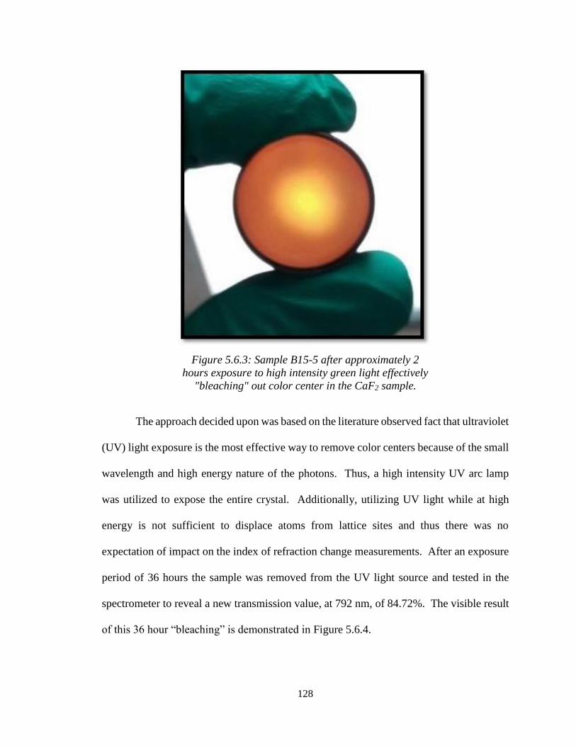
128
Figure 5.6.3: Sample B15-5 after approximately 2
hours exposure to high intensity green light effectively
"bleaching" out color center in the CaF2 sample.
The approach decided upon was based on the literature observed fact that ultraviolet
(UV) light exposure is the most effective way to remove color centers because of the small
wavelength and high energy nature of the photons. Thus, a high intensity UV arc lamp
was utilized to expose the entire crystal. Additionally, utilizing UV light while at high
energy is not sufficient to displace atoms from lattice sites and thus there was no
expectation of impact on the index of refraction change measurements. After an exposure
period of 36 hours the sample was removed from the UV light source and tested in the
spectrometer to reveal a new transmission value, at 792 nm, of 84.72%. The visible result
of this 36 hour “bleaching” is demonstrated in Figure 5.6.4.
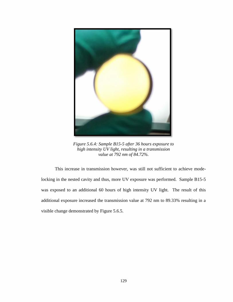
129
Figure 5.6.4: Sample B15-5 after 36 hours exposure to
high intensity UV light, resulting in a transmission
value at 792 nm of 84.72%.
This increase in transmission however, was still not sufficient to achieve mode-
locking in the nested cavity and thus, more UV exposure was performed. Sample B15-5
was exposed to an additional 60 hours of high intensity UV light. The result of this
additional exposure increased the transmission value at 792 nm to 89.33% resulting in a
visible change demonstrated by Figure 5.6.5.

130
Figure 5.6.5: Sample B15-5 after a total of 96 hours of
exposure to high intensity UV light, resulting, in an
transmission value at 792 nm of 89.33%.
After this additional exposure, the nested cavity was right on the verge of mode-
locking at 792 nm but even with increase laser power output it wasn’t quite able to achieve
mode-locking. However, with these three data points for transmission and exposure time
to UV irradiation an estimation of the This increase in transmission however, was still not
sufficient to achieve mode-locking in the nested cavity and thus, more UV exposure was
needed. However, due to the failure of the 200 W helium-xenon arc lamp it could not be
completed as part of this work. Although, through a simple logarithmic calculation an
estimate of the required exposure time was determined to be about 310 total hours exposure
to a 200 W helium-xenon arc lamp in order to restore the sample closely to its original
transmission state. Sample B15-5 was exposed to a total of approximately 276 hours of
UV light at which mode-locking was able to occur after reaching a transmission percentage
of 91.11%.
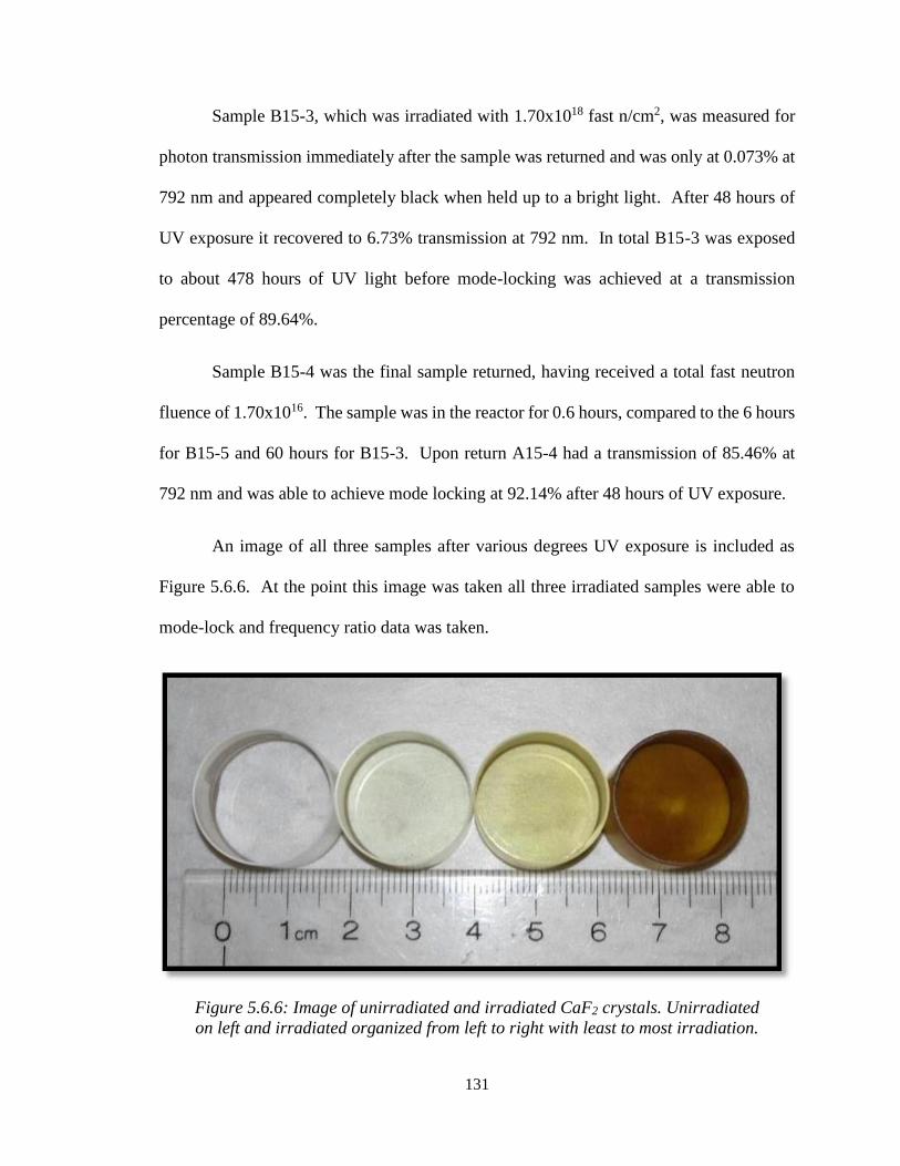
131
Sample B15-3, which was irradiated with 1.70x10¹⁸ fast n/cm2, was measured for
photon transmission immediately after the sample was returned and was only at 0.073% at
792 nm and appeared completely black when held up to a bright light. After 48 hours of
UV exposure it recovered to 6.73% transmission at 792 nm. In total B15-3 was exposed
to about 478 hours of UV light before mode-locking was achieved at a transmission
percentage of 89.64%.
Sample B15-4 was the final sample returned, having received a total fast neutron
fluence of 1.70x10¹⁶. The sample was in the reactor for 0.6 hours, compared to the 6 hours
for B15-5 and 60 hours for B15-3. Upon return A15-4 had a transmission of 85.46% at
792 nm and was able to achieve mode locking at 92.14% after 48 hours of UV exposure.
An image of all three samples after various degrees UV exposure is included as
Figure 5.6.6. At the point this image was taken all three irradiated samples were able to
mode-lock and frequency ratio data was taken.
Figure 5.6.6: Image of unirradiated and irradiated CaF2 crystals. Unirradiated
on left and irradiated organized from left to right with least to most irradiation.

132
From these measurements, refractive index change was calculated and after
applying the overall uncertainty Figure 5.6.7 demonstrates the results of the OSU
irradiation experiments.
Figure 5.6.7: Refractive index change measurement results from OSU irradiated
samples. B15-4 was irradiated to 1.99x10⁴ Gy. B15-5 was irradiated to 1.99x10⁵ Gy.
B15-3 was irradiated to 1.99x10⁶ Gy.
The data shown in Figure 5.6.7 demonstrates an overall downward trend in the data
despite the results from B15-4. However, still due to the uncertainties a definitive
refractive index change cannot be stated because of the small amount of refractive index
change measured. Additional irradiations at higher neutron fluence, or a more thorough
examination of the causes of the daily uncertainty, are required to confirm this trend in the
data the results of the OSU irradiation experiments.
-1.00E-04
-7.50E-05
-5.00E-05
-2.50E-05
0.00E+00
2.50E-05
5.00E-05
-5.00E+05 0.00E+00 5.00E+05 1.00E+06 1.50E+06 2.00E+06 2.50E+06 3.00E+06
Ref
ract
ive I
nd
ex C
han
ge
(Δn
)
Absorbed Dose (Gy)
np Change in OSU Irradiated CaF2 Samples

133
5.7 Combining Experiment Results
An important aspect of this research is the universal nature of measuring and
relating the change in refractive index to a definable standard quantity within the nuclear
realm. This is shown in Primak’s work as a function of neutron fluence (n/cm2) [5].
However, this is a somewhat deceptive quantity to correlate with refractive index change
because as the modeling and simulation portion of this research has shown the energy of
the neutron is a very important quantity, with number of displacements increasing with
energy. Simply correlating refractive index change to neutron fluence the energy is
erroneously ignored. If only neutron fluence was used, separate types of irradiation could
never be compared or fit into the model unless they share and identical energy neutron
source. If, however, a quantity including energy is utilized a model for refractive index
change could be shared among different irradiation sources.
The ideal quantity for overall comparison is absorbed dose, the energy absorbed
per mass of target material. Assuming the standard for calculating dose is uniform between
comparisons the utilization of this quantity should enable comparison of refractive index
change in separate samples having been exposed to separate irradiation sources. In the
case of this research, the different irradiation sources are (1) the NH-3 neutron howitzer,
(2) the Sandia D-D and D-T fusion produced neutron source, and (3) the Oregon State
University TRIGA reactor.
To demonstrate this approach a plot was generated showing the refractive index
change against absorbed dose (Figure 5.7.1) as calculated by the kerma factors defined
earlier in Table 4.2.3.

134
Figure 5.7.1: Refractive index change measured in all irradiated CaF2 samples as a
function of absorbed dose.
At first glance Figure 5.7.1 seems to show little correlation in the overall set of data
collected from the various irradiations and measurement taken throughout this work.
However, we will look more closely at this in the next section.
5.8 Data Trends
There are many things to take into account when considering data trends and overall
quality of the full amount of data produced in this work.
The first consideration is expected refractive index change. This goes back to the
Primak experiment with SiO2 [5], the original inspiration for this work. It has been
surmised though the modeling portion of this work and seen in Primak’s experiments that
refractive index decreases as density decreases. However, the neutron fluences experience
in Primak’s work [5] were one to three orders of magnitude greater than those included in
-1.0E-04
-8.0E-05
-6.0E-05
-4.0E-05
-2.0E-05
0.0E+00
2.0E-05
4.0E-05
6.0E-05
1E-02 1E+00 1E+02 1E+04 1E+06
Ref
ract
ive
Ind
ex C
han
ge
(Δn
)
Absorbed Dose (Gy)
np Change Measured Accross All Experimental Results
Original Howitzer Data
Secondary Howitzer Data
Sandia Irradiation Data
OSU Irradiation Data

135
this work. A recreation of the refractive index potion of the crystalline SiO2 from Primak’s
work is shown in Figure 5.8.1 along with two curve fits of the data.
Figure 5.8.1: Recreation of Primak [5] refractive index measurement data.
Figure 5.8.1 shows an exponential interpolation of the Primak data as well as a
linear interpolation of the first two data points. Utilizing these interpolations and assuming
that CaF2 crystals will behave in a similar way to the SiO2 crystals, an estimation of the
expected refractive index can be calculated for the neutron fluences and doses that have
been explored in this research. Give that the overall uncertainty of this work was calculated
to be 2.4x10⁻⁵ in order to witness a refractive index change that is outside of this uncertainty
a minimum fluence of 1.70x10¹⁸ n/cm2 (or dose of 1.99x10⁶ Gy) would have to be incident
on a CaF2 crystal. Sample B15-3 was the only measured sample to have achieved a fast
neutron fluence of 1.70x10¹⁸ n/cm2 and thus if the behavior is similar in CaF2 and SiO2 the
expected refractive index change is -1.022x10⁻⁴ and -3.62x10⁻⁴, for the exponential and

136
linear interpolations, respectively. It should be noted that the measured refractive index
change for sample B15-3 was -5.1x10⁻⁵ ± 2.4x10⁻⁵ which nearly contains the exponentially
derived refractive index change expectation. With regard the rest of the data, per both the
linear and exponential interpolations, anything below a fluence of 1.70x10¹⁸ n/cm2 would
be within the noise of the overall uncertainty.
The next consideration is the overall trend of the data. While it seems from Figure
5.7.1 that a trend would be difficult to extract one must consider that the x-axis is
logarithmic and not linear. Thus, in order to better observe a potential linear data trend
(which would be expected for these small fluence/dose values), a linear plot should be
observed. Included as Figure 5.8.2 is a linear plot of this data with a linear curve fit
followed by a semi-log plot of the data in Figure 5.8.3.

137
Figure 5.8.2: Plot of irradiation data on a linear scale demonstrating a decreasing trend
in refractive index on average. The dotted line represents a linear curve fit of the data.
Figure 5.8.3: Plot of all irradiation data on a semi-log scale.
-1.0E-04
-8.0E-05
-6.0E-05
-4.0E-05
-2.0E-05
0.0E+00
2.0E-05
4.0E-05
6.0E-05
0.0E+00 5.0E+05 1.0E+06 1.5E+06 2.0E+06 2.5E+06 3.0E+06
Ref
ract
ive
Ind
ex C
ha
ng
e (Δ
n)
Absorbed Dose (Gy)
np Change Measured Accross All Experimental Results
All Irradiation Data
Linear (All Irradiation Data)
-1.0E-04
-8.0E-05
-6.0E-05
-4.0E-05
-2.0E-05
0.0E+00
2.0E-05
4.0E-05
6.0E-05
1E-02 1E-01 1E+00 1E+01 1E+02 1E+03 1E+04 1E+05 1E+06 1E+07
Ref
ract
ive
Ind
ex C
ha
ng
e (Δ
n)
Absorbed Dose (Gy)
np Change Measured Accross All Experimental Results

138
It seems that, overall there is a downward trend in the refractive index change
measurements. This is however difficult to state with a large certainty for several reasons.
The relatively low fluence of neutrons results in a low expected refractive index change.
Additionally, the uncertainty of the overall data detracts from being able to definitively
state a downward trend. In order to confirm this trend another irradiation at a fluence
greater than 1018 n/cm2 (corresponding to a dose greater than 1.99 MGy) is necessary or
the overall uncertainty in the data must be decreased and the experiments must be repeated
with a higher accuracy.
Another consideration that could be major factor in the frequency ratio
measurements is the position of the various laser cavity components at the time of
measurement. Due to the natural drift in the laser over time, periodic re-alignments were
necessary and at times major cavity adjustments were required. When considering the NH-
3 Howitzer data. The point at which the data begins to increase for the first time was
directly after a small cavity adjustment and the large jump in the Howitzer data at about
2.5 Gy was directly after a major cavity adjustment in which prisms, focusing mirrors, and
the end mirrors were adjusted. It should be noted that there is the possibility that the major
cavity adjustment has a significant effect on the overall results. Additionally, all the OSU
irradiation measurements were taken after this major cavity adjustment.
However, upon consideration of this fact there seemed to be little information to be
gleaned from this fact especially after plotting both the measurements taken before and
after this change, separately. There was no correlation in the slope of the data between the
before-the-change and after-the-change measurements. It is, nevertheless, still possible

139
that these changes in the cavity parameters can have effects on the frequency ratio and
should be explored further to confirm or rule out any correlation.

140
Chapter 6: Conclusions
There were two primary facets to this research. Each focuses on the change in CaF2
due to neutron irradiations from various sources. The modeling and simulation aspect of
this work focused on the singular atomic scale collisions and their small and medium scale
effects on crystal structure. A further examination was the change in refractive index of a
crystal due to experimental exposure to neutron irradiation.
6.1 Neutron Damage and Effects Modeling
The results of the modeling and simulation portion of this research were limited in
their applicability due to the inability to span the gap of the meso-scale within the time
constraints of the current work. However, the research into single PKA damage cascade
provides enlightenment into radiation damage cascades within CaF2. CaF2’s crystalline
structure, provides self-annealing properties on the picosecond scale. Through the
examination of the damage cascades it was determined that the crystalline structure of CaF2
provided a self-annealing of nearly 90% of the maximum displacements created. This
means the crystal structure allows for 90% of the maximum displacements to either return
to their original lattice site or be replaced by another atom of the same type. Prior to this
work, the determination of the TDE of Ca and F atoms in CaF2 had not been done utilizing
molecular dynamics simulations, and as such is a valuable determination for the future of
CaF2 radiation damage research. In the end, the molecular dynamics analysis confirms a
linear increase in the damage associated with a crystalline FPE with the energy of the
incident neutrons in a PKA energy range from 100 eV to 5 keV.

141
6.2 Crystal Irradiation and Refractive Index Tracking
The results of the experimental aspect of this research are less than exciting but
certainly intriguing. Refractive index change measurements were completed for a variety
of irradiations performed in three different experimental apparatuses. Due to the current
overall uncertainty calculated for this method many of the data points acquired were unable
to be distinguished from the uncertainty noise. Additionally, the inevitability of periodic
cavity re-alignments and the necessity of one major cavity adjustment in this work may
have contributed to an additional error in the OSU data and the tail end of the NH-3 Neutron
Howitzer Data. It was shown that the data point for B15-3, irradiated in the OSU TRIGA
reactor was the only sample to achieve a fluence great enough to, in theory, change the
refractive index beyond the overall uncertainty. However, potentially due to the
aforementioned cavity adjustment, the OSU data appeared to have a refractive index
change that was less than expected. When considering a linear scale there is certainly a
downward trend in the data but in order to confirm this trend additional irradiations at
fluences greater than 1.70x10¹⁸ are required. Additionally, a thorough examination of the
effect of major and minor cavity adjustments are required for future exploration of this
method as well as causes of the high overall uncertainly in measurement.
Regardless, an uncertainty of 2.4x10⁻⁵ (potentially smaller with further
examination) in refractive index change measurements is a significant achievement in and
of itself. This inevitably demonstrates an exceptional stability of the measurement
technique, and testifies to the precision of this type of dosimetry with crystal FPEs.

142
Chapter 7: Future Work
7.1 Meso-Scale Modeling and Refractive Index Change Prediction
The focus of simulations was on a thorough modeling of the displacement thresholds
of individual Ca and F atoms in CaF2. This is extremely important as most damage is
microscopic, and this contributes to most of the radiation effects [1]. It would be useful to
be able to predict measurable bulk effects stemming from the small-scale effects. Future
work applicable to this research could include bridging this gap utilizing theory developed
and demonstrated by Norget, Torrens, and Robinson (NRT) [27] and also Nucleation Rate
Theory [64]. By utilizing the parameters in this research, namely, the Threshold
Displacement Energy values as well as the atomic binding energy values, a more applicable
form of modeling can be completed. From here, a correlation could be made enabling a
modeling and simulation based prediction of refractive index change due to specified
neutron irradiation. Another useful examination would be utilizing MCNP to determine
neutron particle track information (PTRAC) that can be exported to programs like SRIM
to model the full-scale damage cascades caused by all the neutrons interacting in CaF2 for
a specific irradiation.
7.2 Irradiation Experimentation
It is expected that further irradiation experiments will continue to examine the
correlation demonstrated in this research further. Being able to trace the change of
refractive index all the way to the point it is rendered amorphous of the crystal due to
irradiation damage would provide a full analysis of CaF2. Additionally, CaF2 is just one
of a large set of materials that can be utilized for this type of dosimetry. This work could
143
be repeated both in modeling, simulation, and experiment with a variety of crystals.
Readily available, commercially produced FPE windows include sapphire, other fluoride
compounds and crystalline quartz. Early examination of CaF2 samples irradiated at OSU
showed strong color center formation and darkening of the material. This is expected as
halides are used for optically stimulated luminescence dosimeters which rely on trapped
electron states. This provides an electron effect based mode for examining ionizing
radiation, but non-darkening crystals would make refractive index measurements easier.
Expanding beyond this work to include other crystal types will further demonstrate the
viability of utilizing these techniques in neutron dosimetry applications.
7.3 Fiber Analysis
In order to approach the goal of real time analysis while a sample is being irradiated
the laser cavity will need to be refined, minimized, and made portable or at the very least
semi-portable. One way that this can be accomplished is by utilizing optical fibers and
solid state lasers. The coupling and development of this would be another full dissertation
in and of itself. However, it is a topic that needs to be considered for applying this
technique to neutron dosimetry. The implementation of this research is limited in nature
unless a development of a more portable version of this technique can be developed.
7.4 Uncertainty and Error Analysis
It has been made clear throughout this work that a thorough uncertainty and error
analysis is needed to decrease the overall uncertainty that made the measurement of
refractive index change so difficult in this research. This can be accomplished through a
periodic changing of cavity parameters while tracking the frequency ratio change.

144
Additionally, a thorough analysis of the correlation of the laboratory environment should
be completed to assess a more direct correlation between the laboratory environment and
the frequency ratio drift.
7.5 Additional Irradiation and Crystal Variety
Lastly, due to the darkening of CaF2 crystals at fast neutron fluences above 1016 it
will be difficult to continue to higher fluences with CaF2. Therefore another material must
be considered. Fortunately, the change in refractive index effect is expected to be similar
for all crystalline materials and thus there are many materials from which to chose. Two
of the most readily available optical windows (to act as an FPE) are crystalline SiO2 and
AlO3. Continuing to higher neutron fluences and doses in either of these crystals would be
extremely beneficial in further validating this work.
145
References
[1] C. Dethloff, E. Gaganidze and J. Aktaa, "Quantitative TEM analysis of precipitation
and grain boundary segregation in neutron irradiated EUROFER 97," Journal of
Nuclear Materials, vol. 454, pp. 323-331, 2014.
[2] S. Zinkle and E. Hodgson, "Radiation-induced changes in the physical properties of
ceramic materials," Journal of Nuclear Materials, vol. 191, no. A, pp. 58-66, 1992.
[3] A. Sand, S. Dudarev and K. Kordlund, "High-energy collision cascades in tungsten:
Dislocation loops structure and clustering scaling laws," EPL, vol. 103, no. 46003,
2013.
[4] X. Yi, A. Sand, D. Mason, M. Kirk, S. Roberts, K. Kordlund and S. Dudarev, "Direct
observation of size scaling and elastic interaction between nano-scale defects in
collision cascades," EPL, vol. 110, no. 36001, 2015.
[5] W. Primak, "Fast-Neutron-Induced Changes in Quartz and Vitreous Silica," Physical
Review, vol. 110, no. 6, pp. 1240-1254, 1958.
[6] S. Girard, J. Kuhnhenn, A. Gusarov, B. Brichard, M. Ban Uffelen, Y. Ouerdane, A.
Boukenter and C. Marcandella, "Radiation Effects on Silica-Based Optical Fibers:
Recent Advances and Future Challenges," IEEE Transactions of Nuclear Science,
vol. 60, no. 3, pp. 2015-2036, 2013.
[7] A. I. Gusarov, D. Doyle, A. Hermanne, F. Berghmans, M. Fruit, G. Ulbrich and M.
Blondel, "Refractive-Index Changes Caused by Proton Radiation in Silicate Optical
Glasses," Applied Optics, vol. 41, no. 4, pp. 678-684, 2002.
[8] K. Masuda, "Intracavity coherent interaction of mode-locked pulse train with resonant
medium," Doctoral Dissertation, University of New Mexico, 2014.
[9] K. Masuda and A. Hecht, "Novel techniques for high precision refractive index
measurements, and application to assessing neutron damage and dose in crystals,"
Nuclear Instruments and Methods in Physics Research A, vol. 784, pp. 198-201,
2015.
[10] G. Cheymol, H. V. J.-F. Long and B. Brichard, "High Level Gamma and Neutron
Irradiation of Silica Optical Fibers in CEA OSIRIS Nuclear Reactor," IEEE
Transactions on Nuclear Science, vol. 55, no. 4, pp. 2252-2258, 2008.
[11] S. Plimpton, "Fast Parallel Algorithms for Short-Range Molecular Dynamics," J
Comp Physics, vol. 117, pp. 1-19, 1995.
146
[12] H. D. Holland, "The Effect of Nuclear Radiation on the Structure of Zircon," Acta
Crystallographica, vol. 8, pp. 291-300, 1955.
[13] D. R. Orlander, Fundamental Aspects of Nuclear Reactor Fuel Elements, United
States: Technical Information Center, Office of Public Affairs, Energy Research and
Development Administration, 1976.
[14] S. Tavernier, "Interaction of Particles in Matter," in Experimental Techniques in
Nuclear and Particle Physics, Springer Berlin Heidelberg, 2010, pp. 23-53.
[15] S. Tavernier, Experimental Techniques in Nuclear and Particle Physics, Heidelberg:
Springer, 2010.
[16] C. A. Becker, "Interatomic Potentials Repository Project," NIST - Material
Measurement Laboratory, 13 May 2016. [Online]. Available:
http://www.ctcms.nist.gov/potentials/. [Accessed 27 May 2016].
[17] C. A. Becker, F. Tavazza, Z. T. Trautt and R. A. Barque de Macedo, "Considerations
for choosing and using force fields and interatomic potentials in materials science and
engineering," Frontiers in Methods for Materials Simulations, vol. 17, no. 6, pp. 277-
283, 2013.
[18] I. Malitson, "A Redetermination of Some Optical Properties of Calcium Fluoride,"
Applied Optics, vol. 2, no. 11, pp. 1103-1107, 1963.
[19] O. Heavens, Optical Properties of Thin Solid films, New York: Dover Publications,
Inc., 1991.
[20] B. J. Cowen and M. S. El-Genk, "On force fields for molecular dynamics simulations
of crystalline silica," Computational Materials Science, vol. 107, pp. 88-101, 2015.
[21] R. S. Averback and T. Diaz de la Rubia, "Displacement Damage in Irradiated Metals
and Semiconductors," Solid State Physics, vol. 51, pp. 281-402, 1998.
[22] C. Erginsoy, G. H. Vineyard and A. Englert, "Dynamics of Radiation Damage in a
Body-Centered Cubic Lattice," Physical Review, vol. 133, no. 2A, pp. A595-A606,
1964.
[23] M.-J. Caturla, D. L. Rubia, T. Diaz and G. Gilmer, "Point defect Production,
Geometry and Stability in Silicon: a Molecular Dynamics Simulation Study,"
Symposium A – Materials Synthesis and Processing Using Ion Beams, vol. 316, pp.
141-146, 1993.

147
[24] L. Malerba and J. M. Perlado, "Basic mechanisms of atomic displacement production
in cubic silicon carbide: A molecular dynamics study," Physical Review B, vol. 65,
no. 4, p. 045202, 2002.
[25] W. Windl, T. J. Lenosky, J. D. Kress and F. V. Arthur, "First-principles investigation
of radiation induced defects in Si and SiC," Nuclear Instruments and Methods in
Physics Research B, vol. 141, pp. 61-65, 1998.
[26] E. Holmstrom, A. Kuronen and K. Nordlund, "Threshold defect production in silicon
determined by density functional theory molecular dynamics simulations," Physical
Review B, vol. 78, no. 4, p. 045202, 2008.
[27] M. J. Norgett, M. T. Robinson and I. M. Torrens, "A proposed method of calculating
displacement dose rates," Nuclear Engineering and Design, vol. 33, no. 1, pp. 50-54,
1975.
[28] A. E693-12, "Standard Practice for Characterizing Neutron Exposures in Iron and
Low Alloy Steels in Terms of Displacements Per Atom (DPA)," ASTM International,
Conshohocken, 2012.
[29] B. J. Cowen and M. S. El-Genk, "Probability-based threshold displacement energies
for oxygen and silicon atoms in a-quartz silica," Computational Materials Science,
vol. 117, pp. 164-171, 2016.
[30] D. Chen, "Molecular Dynamics Simulation of Damage Cascade Formation in Ion
Bombarded Solids," Masters Thesis, Texas A&M University, 2011.
[31] N. A. Capps, "Molecular Dynamics Simulations of Cascade Evolution near Pre-
Existing Defects," Masters Thesis, University of Tennessee, 2013.
[32] G. Kinchin and R. Pease, "The Displacement of Atoms in Solids by Radiation,"
Reports on Progress in Physics, vol. 18, pp. 1-51, 1955.
[33] J. Brinkman, "Production of Atomic Displacements by High-Energy Particles,"
American Journal of Physics, vol. 24, pp. 246-267, 1956.
[34] A. Seeger, "On the Theory of Radiation Damage and Radiation Hardening," in
Proceedings of the Second United Nations International Conference on the Peaceful
Uses of Atomic Energy, Geneva, 1958.
[35] OECD/NEA, "Primary Radiation Damage in Materials," OECD/NEA,
https://www.oecd-nea.org/science/docs/2015/nsc-doc2015-9.pdf, 2015.

148
[36] M. Gillan, "Collective dynamics in super-ionic CaF2: I. Simulation compared with
neutron-scattering experiment," J. Phys. C: Solid State Phys., vol. 19, pp. 3391-3411,
1986.
[37] N. de Leeuw and T. Cooper, "A computational study of the surface structure and
reactivity of calcium fluoride," J. Mater. Chem., vol. 13, pp. 93-101, 2003.
[38] K. Fa, A. Nguyen and J. Miller, "Hydrophobic Attraction As Revealed by AFM Force
Measurements and Molecular Dynamics Simulation," J. Phys. Chem. B, vol. 109, pp.
13112-13118, 2005.
[39] S. Vyas, R. Grimes, V. Bulatov and M. Abramowski, "The Surface Structure of CaF2;
A Comparison of Techniques," Molecular Simulation, vol. 26, pp. 307-321, 2001.
[40] M. W. Cooper, M. J. Rushton and R. W. Grimes, "A many-body potential approach
to modelling the thermomechanical properties of actinide oxides," Journal of Physics:
Condensed Matter, vol. 26, no. 10, 2014.
[41] M. L. Goldberger and K. M. Watson, Collision Theory, New York City: John Wiley
& Sons, Inc., 1964.
[42] L. T. Chadderton, Radiation Damage in Crystals, London: Methuen & Co Ltd., 1965.
[43] R. Johnson and A. Orlov, Physics of Radiation Effects in Crystals, Amsterdam:
Elsevier Science Publishers B.V., 1986.
[44] D. S. Billington and J. H. Crawford, Radiation Damage in Solids, Princeton:
Princeton University Press, 1961.
[45] L. T. Chadderton and I. McC.Torrens, Fission Damage in Crystals, London: Methuen
& Co Ltd, 1969.
[46] S. O. Kasap, Optoelectronics and Photonics: Priciples and Practices, Upper Saddle
River, NJ: Prentice-Hall, Inc., 2001.
[47] E. Hecht, Optics, Pearson Education, Inc., 2017.
[48] P. W. Smith, "Mode-Locking of Lasers," Proceedings of the IEEE, vol. 58, no. 9, pp.
1342-1355, 1970.
[49] J.-C. Diels, Ultrashort Laser Pulse Phenomena, Albuquerque: Elsevier Inc., 2006.
[50] J. Ye and S. T. Cundiff, Femtosecond optical frequency comb: principle, operation,
and applications, Norwell, MA: Springer, 2005.

149
[51] A. Lipson, S. Lipson and H. Lipson, Optical Physics, Cambridge University Press,
2010.
[52] K. Masuda, J. Hendrie, J.-C. Diels and L. Arissian, "Envelope, group, and phase
velocities in a nested frequency comb," Journal of Physics B: Atomic, Molecular and
Optical Physics, vol. 49, p. 095401, 2016.
[53] K. Zhao, Q. Zhang, M. Chini, Y. Wu, X. Wang and Z. Chang, "Tailoring a 67
attosecond pulse through advantageous phase-mismatch," Optical Letters, vol. 37, no.
18, pp. 3891-3893, 2012.
[54] J. Diels, J. Fontaine and F. Simoni, "Phase Sensitive Measurement," in Proceedings
of the International Conf. on Lasers, McLean, VA, 1983.
[55] J.-C. M. Diels, J. J. Fontaine, I. C. McMichael and F. Simoni, "Control and
measurement of Ultrashort Pulse Shapes (in amplitude and phase) with femtosecond
accuracy," Applied Optics, vol. 24, no. 9, pp. 1270-1282, 1985.
[56] N. Corporation, "CMA Data Sheet," 2012.
[57] C. Ruiz, G. Chandler, G. F. D. Cooper, K. Hahn, R. Leeper, B. McWatters, A. Nelson,
R. Smelser, C. Snow and J. Torres, "Progress in obtaining an absolute calibration of
a total deuterium–tritium neutron yield diagnostic based on copper activation,"
Review of Scientific Instruments, vol. 83, no. 10D913, 2012.
[58] C. Ruiz, R. Leeper, F. Schmidlapp, G. Cooper and D. Malbrough, "Absolute
calibration of a total yield indium activation detector for DD and DT," Review of
Scientific Instruments, vol. 63, no. 10, pp. 4889-4891, 1992.
[59] Z. R. Harvey, "Neutron flux and energy characterization of a plutonium-beryllium
isotopic neutron source by Monte Carlo simulation with verification by neutron
activation analysis," Master's Thesis, UNLV, 2010.
[60] H. Vega-Carrillo, V. Hernandez-Davila, T. Rivera-Montalvo and A. Sanchez,
"Characterization of a 239PuBe Isotopic Neutron Source," in Proceedings of the
ISSSD 2012, 2012.
[61] F. H. Attix, Introduction to Radiological Physics and Radiation Dosimetry, New
York, New York: John Wiley & Sons, Inc, 1986.
[62] R. Caswell, J. Coyne and M. Randolph, "Kerma Factors of Elements and Compounds
for Neutron Energies Below 30 MeV," Int. J. Appl. Radiat. Isot., vol. 33, pp. 1227-
1262, 1982.
[63] NCRP-38, "Protection Against Neutron Radiation (1971)," NCRP, Bethesda, 1971.

150
[64] G. Was, Fundamentals of Radiation Materials Science: Metals and Alloys, New York:
Springer, 2017.
[65] K. Birch and M. Downs, "An Updated Edlén Equation for the Refractive Index of
Air," Metrologia, vol. 30, pp. 155-162, 1993.

151
Appendix A
A.1 LAMMPS TDE Equilibration Input File
# ============== Initialization ==============
units metal
dimension 3
boundary p p p
atom_style charge #sphere
# ============== Atom Definition ==============
lattice fcc 5.462
# From R. W. G. Wyckoff, Crystal Structures, 9th ed. (Interscience/John Wiley, New
# York, 1963), Vol. 1.
region CaF2Lattice block 0 1 0 1 0 1
create_box 2 CaF2Lattice
create_atoms 1 single 0 0 0
create_atoms 1 single 1 0 0
create_atoms 1 single 1 1 0
create_atoms 1 single 0 1 0
create_atoms 1 single .5 .5 0
create_atoms 1 single .5 0 .5
create_atoms 1 single 0 .5 .5
create_atoms 1 single 1 .5 .5
create_atoms 1 single .5 1 .5
create_atoms 1 single 0 0 1
create_atoms 1 single 1 0 1
create_atoms 1 single 1 1 1
create_atoms 1 single 0 1 1

152
create_atoms 1 single .5 .5 1
create_atoms 2 single .25 .25 .25
create_atoms 2 single .25 .75 .25
create_atoms 2 single .75 .25 .25
create_atoms 2 single .75 .75 .25
create_atoms 2 single .25 .25 .75
create_atoms 2 single .25 .75 .75
create_atoms 2 single .75 .25 .75
create_atoms 2 single .75 .75 .75
replicate 6 6 6
mass 1 40.0
mass 2 19.0
set type 1 charge 2.0
set type 2 charge -1.0
# ============== Force Fields ==============
pair_style hybrid/overlay table linear 15000 coul/long 15
kspace_style pppm 1e-5
pair_coeff 1 1 table Pot15_CaCa.lmptab Ca-Ca
pair_coeff 1 2 table Pot15_CaF.lmptab Ca-F
pair_coeff 2 2 table Pot15_FF.lmptab F-F
pair_coeff * * coul/long
# ============== Groups ==============
region rallatoms block 0 6 0 6 0 6
region rexterior block 1 5 1 5 1 5 side out
region rinterior block 1 5 1 5 1 5

153
region rinterior2 block 2 4 2 4 2 4
group crystal region rallatoms
group exterior region rexterior
group interior region rinterior
group in2_4 region rinterior2
# ============== Initialization ==============
compute 1 all temp
compute 2 all coord/atom 5.0
compute 3 all ke/atom
compute eng all pe/atom
compute eatoms all reduce sum c_eng
# ============== Equilibration ==============
velocity crystal create 3.0 4928459
fix 1 all npt temp 293 293 .1 aniso .83993 .83993 1 #ABQ pressure = ~.83993 Bar
timestep 0.001
thermo 100
thermo_style custom step temp pe etotal press atoms vol density lx ly lz c_eatoms
dump id all custom 1000 dumpAll.dump mass type id x y z
dump id2 in2_4 custom 1000 dump2_4.dump mass type id x y z
#+200000 Equil
run 200000
variable natoms equal "count(all)"
variable teng equal "c_eatoms"
variable length equal "lx/6"

154
variable ecoh equal "v_teng/v_natoms"
print "Total energy (eV) = ${teng};"
print "Number of atoms = ${natoms};"
print "Lattice constant (Angstoms) = ${length};"
print "Cohesive energy (eV) = ${ecoh};"
print "Equilibration Completed!"
undump id
undump id2
unfix 1
write_restart 6xEquil.restart
A.2 LAMMPS TDE Input File (Example)
# Looped TDE calc
variable i loop 500
label loop_i
clear
log 20eV_all.log append
print "Running simulation 20eV $i"
variable s equal 'floor(random(10,100000,1000))'
print "Random Seed = $s"
read_restart 6xEquil.restart
# ============== Force Fields ==============
pair_style hybrid/overlay table linear 15000 coul/long 15
kspace_style pppm 1e-5
pair_coeff 1 1 table Pot15_CaCa.lmptab Ca-Ca

155
pair_coeff 1 2 table Pot15_CaF.lmptab Ca-F
pair_coeff 2 2 table Pot15_FF.lmptab F-F
pair_coeff * * coul/long
# ============== Groups ==============
group PKA id 1549 # Define PKA as a Ca atom (different for F TDE calc)
# ============== Initialization ==============
variable t equal "random(0,6.283185307,1000)"
variable p equal "random(0,3.141592654,1000)"
variable theta equal $t
variable phi equal $p
print "Theta (rad) = ${theta}"
print "Phi (rad) = ${phi}"
variable mkg equal '40.078 * 1.66054E-24 / 1000'
variable Ej equal '20 * 1.60218E-19'
variable speed equal 'sqrt(2 * v_Ej / v_mkg) * 0.01'
print "Energy (eV) = ${Ej}"
print "Mass (kg) = ${mkg}"
print "Speed (A/ps) = ${speed}"
variable x equal v_speed*cos(v_theta)*cos(v_phi)
variable y equal v_speed*sin(v_theta)*cos(v_phi)
variable z equal v_speed*sin(v_phi)
print "Velocity (A/ps) in X = $x"
print "Velocity (A/ps) in Y = $y"
print "Velocity (A/ps) in Z = $z"
compute 1 all temp
compute 2 all coord/atom 5.0
156
compute 3 all ke/atom
compute eng all pe/atom
compute eatoms all reduce sum c_eng
compute disp all displace/atom
# ============== Atomic Randomization ==============
dump 20eV PKA custom 20000 20eVPKA.dump mass type id x y z vx vy vz c_disp[4]
dump_modify 20eV append yes
velocity all create 293 $s
fix 1 crystal npt temp 293 293 .1 aniso .83993 .83993 1 #ABQ pressure = ~.83993 Bar
timestep .001
thermo 200
thermo_style custom step time dt temp pe etotal press atoms vol density lx ly lz c_eatoms
run 2000
unfix 1
velocity PKA set v_x v_y v_z
timestep 0.000005
fix 5 all dt/reset 10 1.0e-6 0.00008 .0008
# ============== 15000 Run ==============
fix 1 exterior npt temp 293 293 .1 aniso .83993 .83993 1 #ABQ pressure = ~.83993
Bar
fix 2 interior nve
run 18000
variable natoms equal "count(all)"

157
variable teng equal "c_eatoms"
variable length equal "lx/6"
variable ecoh equal "v_teng/v_natoms"
print "Total energy (eV) = ${teng};"
print "Number of atoms = ${natoms};"
print "Lattice constant (Angstoms) = ${length};"
print "Cohesive energy (eV) = ${ecoh};"
unfix 1
unfix 2
next i
jump Ca20eV.in loop_i
A.3 LAMMPS Cascade Equilibration Input File
# ============== Initialization ==============
units metal
dimension 3
boundary p p p
atom_style charge #sphere
# ============== Atom Definition ==============
lattice fcc 5.444
region CaF2Lattice block 0 1 0 1 0 1
create_box 2 CaF2Lattice
create_atoms 1 single 0 0 0
create_atoms 1 single 1 0 0

158
create_atoms 1 single 1 1 0
create_atoms 1 single 0 1 0
create_atoms 1 single .5 .5 0
create_atoms 1 single .5 0 .5
create_atoms 1 single 0 .5 .5
create_atoms 1 single 1 .5 .5
create_atoms 1 single .5 1 .5
create_atoms 1 single 0 0 1
create_atoms 1 single 1 0 1
create_atoms 1 single 1 1 1
create_atoms 1 single 0 1 1
create_atoms 1 single .5 .5 1
create_atoms 2 single .25 .25 .25
create_atoms 2 single .25 .75 .25
create_atoms 2 single .75 .25 .25
create_atoms 2 single .75 .75 .25
create_atoms 2 single .25 .25 .75
create_atoms 2 single .25 .75 .75
create_atoms 2 single .75 .25 .75
create_atoms 2 single .75 .75 .75
replicate 60 60 60
mass 1 40.0
mass 2 19.0
set type 1 charge 2.0
set type 2 charge -1.0
# ============== Force Fields ==============

159
pair_style table/gpu linear 65536 pppm
kspace_style pppm 1.0e-3
pair_coeff 1 1 CaF2GPUAll.table CaCa
pair_coeff 1 2 CaF2GPUAll.table CaF
pair_coeff 2 2 CaF2GPUAll.table FF
pair_write 1 1 65536 r 0.06 6.5 CCAll.txt CaCa 2 2
pair_write 1 2 65536 r 0.06 6.5 CFAll.txt CaF 2 -1
pair_write 2 2 65536 r 0.06 6.5 FFAll.txt FF -1 -1
# ============== Groups ==============
region rallatoms block 0 60 0 60 0 60
region rinterior block 3 57 3 57 3 57
region rexterior block 3 57 3 57 3 57 side out
region rinterior2 block 15 45 15 45 15 45
region rinterior3 block 20 40 20 40 20 40
group crystal region rallatoms
group interior region rinterior
group exterior region rexterior
group in15_45 region rinterior2
group in20_40 region rinterior3
# ============== Initialization ==============
compute 1 all temp
compute 2 all coord/atom 5.0 #all to interior
compute 3 all ke/atom #all to interior
compute eng all pe/atom
compute eatoms all reduce sum c_eng

160
# ============== Equilibration ==============
velocity crystal create 3.0 4928459
fix 1 all npt temp 293 293 .1 aniso .83993 .83993 1 #ABQ pressure = ~.83993 Bar
timestep 0.0005
thermo 100
thermo_style custom step temp pe etotal press atoms vol density lx ly lz c_eatoms
dump id all custom 5000 dumpAll.dump mass type id x y z vx vy vz
dump id2 in15_45 custom 5000 dump15-45.dump mass type id x y z vx vy vz
dump id3 in20_40 custom 5000 dump20-40.dump mass type id x y z vx vy vz
#+10000 Equil
run 10000
variable natoms equal "count(all)"
variable teng equal "c_eatoms"
variable length equal "lx/60"
variable ecoh equal "v_teng/v_natoms"
print "Total energy (eV) = ${teng};"
print "Number of atoms = ${natoms};"
print "Lattice constant (Angstoms) = ${length};"
print "Cohesive energy (eV) = ${ecoh};"
print "Equilibration Completed!"
write_restart 60xEquil.*.restart

161
A.4 LAMMPS Cascade 1000 keV PKA Input File (Example)
read_restart 60xEquil.*.restart
# ============== Force Fields ==============
pair_style table/gpu linear 65536 pppm
kspace_style pppm 1.0e-3
pair_coeff 1 1 CaF2GPUAll.table CaCa
pair_coeff 1 2 CaF2GPUAll.table CaF
pair_coeff 2 2 CaF2GPUAll.table FF
pair_write 1 1 65536 r 0.06 6.5 1000eV-CCAll.txt CaCa 2 2
pair_write 1 2 65536 r 0.06 6.5 1000eV-CFAll.txt CaF 2 -1
pair_write 2 2 65536 r 0.06 6.5 1000eV-FFAll.txt FF -1 -1
# ============== Groups ==============
#region rallatoms block 0 60 0 60 0 60
#region rinterior block 3 57 3 57 3 57
#region rexterior block 3 57 3 57 3 57 side out
#region rinterior2 block 15 45 15 45 15 45
#region rinterior3 block 20 40 20 40 20 40
#region rinterior4 block 25 35 25 35 25 35
#region rinterior5 block 5 55 5 55 5 55
#group crystal region rallatoms
#group interior region rinterior
group PKA id 2138761
# ============== Initialization ==============
compute 1 all temp
162
compute 2 all coord/atom 5.0
compute 3 all ke/atom
compute eng all pe/atom
compute eatoms all reduce sum c_eng
compute disp all displace/atom
# ============== Equilibration ==============
velocity PKA set 0 0 -693.89
timestep 0.0000005
thermo 500
thermo_style custom step time dt temp pe etotal press atoms vol density lx ly lz c_eatoms
dump id1 in5_55 custom 500 1000eV.in5_55.a.dump type id x y z c_disp[4] c_eng c_3
#+260000 Run
fix 1 exterior npt temp 293 293 .1 aniso .83993 .83993 1 #ABQ pressure = ~.83993
Bar
fix 2 interior nve
fix 3 all dt/reset 10 5.0e-7 .0002 .005
run 260000
variable natoms equal "count(all)"
variable teng equal "c_eatoms"
variable length equal "lx/60"
variable ecoh equal "v_teng/v_natoms"
print "Total energy (eV) = ${teng};"
print "Number of atoms = ${natoms};"
print "Lattice constant (Angstoms) = ${length};"

163
print "Cohesive energy (eV) = ${ecoh};"
undump id1
unfix 1
unfix 2
unfix 3
write_restart 1000eVCol.*.restart

164
Appendix B
B.1 Overview
It became apparent during the course of this work that over an extended period of
time there was a noticeable change in the frequency ratio (the primary value used to track
the change in refractive index) beyond the normal standard deviation for the measurements.
Due to the nature of the mode-locked laser cavity there are many factors that could
influence this value change over a large span of days. Given that the majority of the cavity
is filled with air the logical first thing to consider is the ambient laboratory environment.
As it turned out there wasn’t much cause to move beyond this evaluation because there was
a clear pattern displayed in relating these changes to the ambient laboratory environment.
Three laboratory environment variables were tracked consistently throughout this research,
temperature, relative humidity, and absolute pressure. These values were considered
separately initially and then combined to assess the correlation of the changes with air
density and ultimately the refractive index of the air. The data in this appendix corresponds
to the control sample measurements on the same days on which the NH-3 neutron howitzer
irradiated sample (A15-4) was measured to obtain refractive index change.
B.2 Repetition Rate Change with Laboratory Environment Changes
The first correlation to consider was the change in the repetition rate with respect
to ambient laboratory environment changes. As discussed in the main body of this
dissertation the repetition rate of the cavity and the FPE are the essential building blocks
for quantifying refractive index change in a material. As such their change with respect to
the laboratory environment is of great interest. When considering the three variables

165
separately the temperature of the lab was negligible and when plotted against the change
in the repetition rate for both the cavity and the FPE there was no visible correlation.
However, later when considering air density and refractive index change for the air in the
cavity the temperature plays a larger role.
First, the change in the repetition rate of the cavity was considered with respect to
the relative humidity in the lab. The results are depicted in Figure B.1.
Figure B.1: Cavity repetition rate and relative humidity as measured on days the NH-3
Howitzer sample (A15-4) was measured for refractive index change.
The results shown in Figure B.1 are intriguing as they seem to follow an inverse
relationship initially, however, on day 100 and after the relationship is severely diminished.
Additionally, the frequency ratio was depicted with the pressure of the lab in mBar in
Figure B.2.

166
Figure B.2: Cavity repetition rate and relative humidity as measured on days the NH-3
Howitzer sample (A15-4) was measured for refractive index change
The results shown in Figure B.2 show similar behavior to the humidity results with
the exception that they are reversed. The pressure results tended to follow a less consistent
relationship early but around the same time frame as the humidity results the patter shifts
and the repetition rate seems to adopt an inverse relationship to pressure. It appears that
there is no definable relationship with humidity and pressure, alone. to the cavity repetition
rate. It should be noted that Day 221 is excluded from Figure B.1 and Figure B.2 because
of an extreme data jump. This was due to the choice to measure the frequncy ratios at a
larger cavity length to increase stability. Frequency ratio results were not effected but
plotting them here would deminish the ability to observe the correlations of the other data
points. The consideration of the frequncy ratio in Section B.3 will include the data from
221.

167
B.3 FPE Repetition Rate with Laboratory Environment Changes
Second, the change in the repetition rate of the FPE was considered with respect to
the relative humidity and pressure in the lab. It was not expected that the FPE data would
produce any significant correlation, however, the lab environment can certainly affect this
value and as such it must be considered. Figure B.3 and Figure B.4 show the change FPE
repetition rate measured with relative humidity (Figure B.3) and pressure (Figure B.4) as
measured on days that the NH-3 Howitzer sample A15-4 was removed and measured.
Figure B.3: FPE repetition rate and relative humidity as measured on days the NH-3
Howitzer sample (A15-4) was measured for refractive index change.
Figure B.3 shows that the FPE repetition rate varies quite similar to the relative
humidity but it does not follow a strict pattern.

168
Figure B.4: FPE repetition rate and pressure as measured on days the NH-3 Howitzer
sample (A15-4) was measured for refractive index change.
Figure B.3 shows little correlation between humidity and the FPE repetition rate.
Although it seems to track the slope between several points at times. Again this suggests
that humidity and pressure are not the only factors in the change in repetition rates but the
may certainly have a partial correlation.
B.4 Frequency Ratio Delta with Laboratory Environment Changes
The next correlation to consider was the frequency ratio which combines the two
separate repetition rates into a ratio. The frequency ratio is more heavily affected by the
cavity repetition rate because the cavity repetition rate is affected more by the change in
cavity length than the FPE repetition rate. As such, the results shown here are similar in
appearance to Figure B.1 and Figure B.2, although, the results are a bit more dramatic. The
frequency ratio plots for relative humidity and pressure are shown in Figure B.5 and Figure
B.6, respectively.

169
Figure B.5: Frequency ratio and relative humidity as measured on days the NH-3
Howitzer sample (A15-4) was measured for refractive index change.
Figure B.6: Frequency ratio and pressure as measured on days the NH-3 Howitzer
sample (A15-4) was measured for refractive index change.

170
Similar to the cavity repetition rate results vs laboratory environment the humidity
seems to track inversely with the frequency ratio, however, with the additional day 221
data point added back in a clear direct relationship is seen between day 165 and day 221.
The pressure again does not seem to have a correlation through 100 days, however, after
the 100 day point there again appears an indirect correlation. Again, there is no definable
correlation seen here although these plots certainly seem to suggest that both humidity and
pressure have a partial role in the variation that is seen on a day to day basis.
B.5 Frequency Ratio with Air Density and Refractive Index of Air
Due to the nature of the laboratory setup air plays a major role in the determining
of the necessary values to measure refractive index change. Considering the role that open-
air plays in these measurements the properties of the air should be considered. As
humidity, temperature, and pressure have already been considered separately the next step
is to use them to calculate larger properties of air such as the air density and the refractive
index of the air. The calculation of air density for moist air is a standard calculation from
temperature, pressure, and humidity. Calculating refractive index, although, proportional
to air density, is a bit more complicated. It is ultimately determined for the purposes of
this work by the Edlén Equation [65]. This was completed to produce Figure B.7 and
Figure B.8 for air density and refractive index of air, respectively.

171
Figure B.7: Frequency ratio and air density as measured on days the NH-3 Howitzer
sample (A15-4) was measured for refractive index change.
Figure B.8: Frequency ratio and refractive index of air as measured on days the NH-3
Howitzer sample (A15-4) was measured for refractive index change.
Figure B.7 and Figure B.8, while, combining temperature, humidity, and pressure,
did not end up providing a comprehensive look at the daily variation in frequency ratio. In

172
some ways by combining the humidity, temperature and pressure the plots seem to more
consistently track inversely with the frequency ratio. However, there was still no clear and
definitive pattern for which a correction could be adapted. In order to reduce the daily
variation and thus the overall uncertainty of this method a more thorough analysis of the
causes of the daily variation must be completed.