high precision x-ray logn-logs distributions: implications for …xmmssc- · high precision x-ray...

Astronomy & Astrophysics manuscript no. sm˙logNlogS08 c© ESO 2008September 11, 2008

High precision X-ray logN-logS distributions: implications for theobscured AGN population

S. Mateos1, R.S. Warwick1, F. J. Carrera2, G.C. Stewart1, J. Ebrero1,2, R. Della Ceca3, A. Caccianiga3 , R. Gilli4, M.J.Page5, E. Treister6, J.A. Tedds1, M.G. Watson1, G. Lamer7, R.D. Saxton8, H. Brunner9, and C.G. Page1

1 X-ray Astronomy Group, Department of Physics and Astronomy, Leicester University, Leicester LE1 7RH, UK2 Instituto de Fısica de Cantabria (CSIC-UC), 39005 Santander, Spain3 INAF-Osservatorio Astronomico di Brera, via Brera 28, I-20121 Milan, Italy4 Istituto Nazionale di Astrofisica (INAF) - Osservatorio Astronomico di Bologna, via Ranzani 1, 40127 Bologna, Italy5 Mullard Space Science Laboratory, University College London, Holmbury St. Mary, Dorking, Surrey RH5 6NT, UK6 European Southern Observatory, Casilla 19001, Santiago 19, Chile7 Astrophysikalisches Institut Potsdam, An der Sternwarte 16, 144482, Potsdam, Germany8 XMM SOC, ESAC, Apartado 78, 28691 Villanueva de la Caada, Madrid, Spain9 Max-Planck-Institut fur Extraterrestrische Physik, Giessenbachstrasse, Garching D-85748, Germany

10 September 2008

ABSTRACT

Context. Our knowledge of the properties of AGN, especially those of optical type-2 objects is very incomplete. Extragalactic sourcecount distributions are dependent on the cosmological and statistical properties of AGN, and therefore provide a direct method ofinvestigating the underlying source populations.Aims. We aim to constrain the extragalactic source count distributions over a broad range of X-ray fluxes and in various energy bandsto test whether the predictions from X-ray background synthesis models agree with the observational constraints provided by ourmeasurements.Methods. We have used 1129 XMM-Newton observations at |b| > 20 covering a total sky area of 132.3 deg2 to compile the largestcomplete samples of X-ray selected objects to date both in the 0.5-1 keV, 1-2 keV, 2-4.5 keV, 4.5-10 keV bands employed in standardXMM-Newton data processing and in the 0.5-2 keV and 2-10 keV energy bands more usually considered in source count studies.Our survey includes in excess of 30,000 sources and spans fluxes from ∼10−15 to 10−12 erg cm−2 s−1 below 2 keV and from ∼10−14 to10−12 erg cm−2 s−1 above 2 keV where the bulk of the CXRB energy density is produced.Results. The very large sample size we obtained means our results are not limited by cosmic variance or low counting statistics. Abreak in the source count distributions was detected in all energy bands except the 4.5-10 keV band. We find that an analytical modelcomprising 2 power-law components cannot adequately describe the curvature seen in the source count distributions. The shape ofthe logN(>S)-logS is strongly dependent on the energy band with a general steepening apparent as we move to higher energies. Thisis due to the fact that non-AGN populations, comprised mainly of stars and clusters of galaxies, contribute up to 30% of the sourcepopulation at energies <2 keV and at fluxes ≥10−13 erg cm−2 s−1, and these populations of objects have significantly flatter sourcecount distributions than AGN. We find a substantial increase in the relative fraction of hard X-ray sources at higher energies, from≥55% below 2 keV to ≥77% above 2 keV. However the majority of sources detected above 4.5 keV still have significant flux below2 keV. Comparison with predictions from the synthesis models suggest that the models might be overpredicting the number of faintabsorbed AGN, which would call for fine adjustment of some model parameters such as the obscured to unobscured AGN ratio and/orthe distribution of column densities at intermediate obscuration.

Key words. surveys– X-rays: general– cosmology: observations– galaxies: active

1. Introduction

The deepest X-ray surveys carried out to date by Chandra(Chandra Deep Field North, CDF-N; Alexander et al. 2003 andChandra Deep Field South, CDF-S; Giacconi et al. 2002, Louet al. 2008) and XMM-Newton (Hasinger et al. 2001) have re-solved up to 90% of the Cosmic X-ray background (CXRB)at energies below ∼5 keV into discrete sources reaching limit-ing fluxes of ∼ 2 × 10−17 erg cm−2 s−1 in the 0.5-2 keV band and∼ 2 × 10−16 erg cm−2 s−1 in the 2-8 keV band (Bauer et al. 2004).

However, above ∼5 keV the fraction of CXRB resolved intosources is substantially lower (see e.g. Worsley et al. 2004,Worsley et al. 2005) although precise estimates are hampered

Send offprint requests to: S. Mateos, e-mail: [email protected]

by the remaining uncertainty in the absolute normalisation ofthe CXRB (see e.g. Cowie et al. 2002). Additional uncertaintiesoriginate due to variations of the source counts between surveysarising from both the impact of the large scale structure of theUniverse on the source distribution (Gilli et al. 2003) and, moremundanely, on cross calibration uncertainties between differentmissions (Barcons et al. 2000, De Luca & Molendi 2004).

Follow-up campaigns targeted at the sources detected indeep-medium X-ray surveys have shown that at high Galacticlatitudes Active Galactic Nuclei (AGN) dominate the X-raysky. At bright X-ray fluxes (& 10−14 erg cm−2 s−1), unabsorbedor mildly absorbed AGN, spectroscopically identified as type-1 AGN represent the bulk of the population (see e.g. Shankset al. 1991, Barcons et al. 2007, Caccianiga et al. 2008).

2 S. Mateos et al.: High precision X-ray logN-logS distributions: implications for the obscured AGN population

Fig. 1. Sky distribution in Galactic coordinates of the selected observa-tions. The high density of pointings in some areas of the sky correspondto planned surveys of relatively large sky areas (e.g. the XMM-NewtonLarge Scale Survey, Pierre et al. 2004).

At intermediate fluxes, absorbed AGN (optical type-2 AGN)at low redshifts (z.1) become dominant, while at fluxes. 10−16 erg cm−2 s−1 a population of ‘normal’ galaxies starts toemerge (Barger et al. 2003, Hornschemeier et al. 2003, Bauer etal. 2004).

Although the nature of the sources that dominate the CXRBis reasonably clear, there are still large uncertainties in the cos-mological and statistical properties of the objects, especially fortype-2 AGN for which the redshift and column density distribu-tions are rather poorly determined to date.

One of the most important open issues regarding the popu-lation of absorbed AGN is whether the relative fraction of ob-scured AGN varies with redshift or X-ray luminosity. Some re-sults suggest that this fraction is independent of the X-ray lu-minosity and redshift (Dwelly & 006), while others pointto a decrease in the fraction of absorbed AGN with the X-rayluminosity (Ueda et al. 2003, Barger et al. 2005, Hasinger etal. 2005, La Franca et al. 2005, Akilas et al. 2006, Della Ceca etal. 2008) and/or an increase with redshift (La Franca et al. 2005,Ballantine et al. 2006, Treister & Urry 2006). This issue has beenrecently investigated by Della Ceca et al. (2008) via the analy-sis of a complete spectroscopically identified (∼97% complete-ness) sample of bright X-ray sources (> 7 × 10−14 erg cm−2 s−1)selected in the 4.5-7.5 keV band. The sources in this study werebright enough to obtain their absorption properties from a de-tailed analysis of their X-ray spectra. They report a dependenceof the fraction of obscured AGN on both the luminosity and red-shift, the measured evolution being consistent with that proposedby Treister & Urry (2006). A dependence of the fraction of ab-sorbed AGN on the luminosity has also been suggested by ob-servations in the optical and mid-infrared (Simpson et al. 2005,Maiolino et al. 2007).

X-ray surveys are the best way to understand the proper-ties (i.e. X-ray absorption distributions) and cosmological evo-lution (i.e. X-ray luminosity functions) of AGN and to test thepredictions of the synthesis models of the CXRB (Treister &Urry 2006, Gilli et al. 2007). However in order to provide strongobservational constraints these analyses require complete sam-ples with a high fraction of sources spectroscopically identi-fied. This is a difficult and very time consuming task that canonly be achieved for relatively small samples of objects. Sourcecount distributions are dependent on the cosmological and sta-tistical properties of AGN, and therefore provide a rather di-rect method of investigating the properties of the underlyingsource populations. Constraining the shape of the source countsis fundamental for cosmological studies of AGN, as it providesstrong observational constraints for the synthesis models of the

CXRB. The general shape of the source counts in the 0.5-2 keVand 2-10 keV bands is well determined from deep and mediumdepth X-ray surveys. The results of these analyses show that atfluxes ∼10−15 − 10−14 erg cm−2 s−1 the source count distributionscan be reproduced well with broken power-law shapes (i.e twopower-law, hereafter broken power-law, Baldi et al. 2002, Cowieet al. 2002, Cappelluti et al. 2007, Carrera et al. 2007, Brunner etal. 2008). However, mostly due to poor statistics, a proper deter-mination of the analytical form of the source count distributionsis still unavailable, especially at high energies.

Deep pencil beam surveys are important to study the popu-lations of sources at the faintest accessible fluxes and thereforethey are best suited to constrain the faint-end slope of the sourcecounts. However these observations only sample small sky ar-eas and therefore suffer from significant cosmic variance. Forexample, the CDF-N and CDF-S source counts deviate by morethan 3.9σ at the faintest flux levels (Bauer et al. 2004). On theother hand, wide shallow surveys cover much larger areas of thesky and therefore are less affected by cosmic variance. However,they only sample sources at relatively bright fluxes which onlycontribute a small fraction of the CXRB emission. Surveys atintermediate fluxes, ∼10−15 − 10−13 erg cm−2 s−1, of the type re-ported here, fill the gap between deep pencil beam and shallowsurveys and sample the fluxes at the break in the source countdistributions, i.e. where the bulk of the CXRB energy densityshould be produced. These surveys are therefore appropriate toaccurately determine the position of the break and bright-endslope of source count distributions.

In this paper we put strong constraints on the analytical shapeof the extragalactic source count distributions in a number ofdifferent energy bands and over a wide range of fluxes. For thispurpose we have compiled the largest complete samples of X-ray selected objects to date, ensuring that our results are not lim-ited by low counting statistics or cosmic variance effects. Takingadvantage of our large samples, we have investigated how theunderlying population of X-ray sources changes as we move tohigher energies. Finally we have used the new observational con-straints provided by our analysis to check the predictions of cur-rent synthesis models of the CXRB.

The paper is organised as follows: In §2 we describe the se-lection and processing of the XMM-Newton observations (§2.1),the source detection procedure and criteria for selection ofsources (§2.2 and §2.3), we discuss how we calculated the fluxesof the sources from their count rates (§2.4) and we explain howthe sky coverage was calculated as a function of the X-ray flux(§2.5). In §3 we describe the different representations of sourcecounts used in this work (§3.1), present source count distribu-tions in different energy bands (§3.2 and §3.3), discuss the im-pact on our source count distributions of biases inherent in oursource detection procedure (§3.4), describe the approach used tofit our distributions (§3.5) and discuss the fractional X-ray back-ground contributed by our sources (§3.6). In §4 we summarisethe X-ray spectral properties of our objects. The implications ofour analysis for the cosmic X-ray background synthesis modelsare presented in §5. Finally, the summary and conclusions of ouranalysis are given in §6. Appendix A describes the empirical ap-proach used to obtain the sky coverage as a function of the X-rayflux. In Appendix B we compare our source count distributionswith those obtained using data taken directly from the 2XMM cat-alogue.

S. Mateos et al.: High precision X-ray logN-logS distributions: implications for the obscured AGN population 3

Fig. 2. Left: Distribution of Galactic hydrogen column density (in log units) along the line of sight taken from the 21 cm radio measurements ofDickey & Lockman (1990). Right: Distribution of the exposure times (after filtering).

2. Data processing and analysis

2.1. The XMM-Newton observations

The observations employed in this study are a subset of thoseutilised in producing the second XMM-Newton serendipitoussource catalogue, 2XMM1 (Watson et al. 2008, submitted). 2XMM isbased on observations from the three European Photon ImagingCameras (EPIC) that were public by first of May 20072. Herefor simplicity, we have only used data from the EPIC pn cam-era (Turner et al. 2001). The data have been processed using theXMM-Newton Science Analysis System (SAS, v7.1.0, Gabrielet al. 2004). Because all the observations have been reprocessedusing the same pipeline configuration this guarantees a uniformdata set. Observations have been filtered for high particle back-ground periods by excluding the time intervals where the 7-15keV count rate was higher than 10 pn cts/arcmin2/ks.

The aim of this study is to constrain source count distribu-tions for serendipitous AGN, hence we have selected only ob-servations that fulfil the following criteria:

1. High galactic latitude fields, |b| > 20 (so as to obtain sam-ples with the contamination from Galactic stars minimisedand with low Galactic absorbing column densities).

2. Fields with at least 5 ks of clean pn exposure time.3. Fields free of bright and/or extended X-ray sources, i.e.

where most of the field of view (FOV) can be used forserendipitous source detection.

We have not merged observations carried out at the same skyposition. In these cases we removed the overlapping area fromthe observation with the shortest clean exposure time. The result-ing sample comprises 1129 observations. The sky distribution ofthe pointings is shown in Fig. 1. The distribution of Galacticabsorption along the line of sight and the distribution of cleanexposure times, for the set of observations are shown in Fig. 2.

2.2. Source detection

We have carried out source count analysis using both the ’stan-dard’ 0.5-2 keV and 2-10 keV energy bands and also the nar-

1 http://xmmssc-www.star.le.ac.uk/Catalogue/2XMM/2 XMM-Newton observations started on January 2000.

rower energy bands 0.5-1 keV, 1-2 keV, 2-4.5 keV and 4.5-10 keV3. The former allow comparison with previous results,whereas the later allow a more detailed study of the spectralcharacteristics of the underlying source populations. In order tomake source lists we run the 2XMM source detection algorithm onall energy bands simultaneously. In Appendix B we compare our0.5-2 keV and 2-10 keV source count distributions with thoseobtained combining data from the energy bands used to makethe 2XMM catalogue.

Images were created for each energy band. Only pn eventswith PATTERN ≤4 (single and double events) were selected. TheSAS task emask was used to create a detection mask for eachobservation, which defines the area of the detector suitable forsource detection. Energy dependent exposure maps were com-puted using the SAS task eexpmap, using the latest calibrationinformation on the mirror vignetting, quantum efficiency andfilter transmission4. Source lists were obtained using the SAStask eboxdetect, which performs source detection using a sim-ple sliding box cell detection algorithm. Background maps wereobtained with the SAS task esplinemap. The sources detected

3 In the 4.5-10 keV band pn photons with energies between 7.8-8.2keV were excluded in order to avoid the instrumental background pro-duced by Cu K-lines (Lumb et al. 2002).

4 Eexpmap calculates the mirror vignetting function at one single en-ergy, the centroid of the energy band. Because the mirror vignetting is astrong function of energy, in the cases where the energy band is broad,this approach produces a less accurate determination of the effective ex-posure across the FOV. This is more important at high energies, wherethe dependence of the vignetting on the energy is much stronger. In or-der to reduce this effect, for the energy bands 0.5-2 keV, 4.5-10 keV and2-10 keV we first computed exposure maps in narrower energy bands:0.5-1 keV and 1-2 keV for band 0.5-2 keV; 2-4.5, 4.5-6 keV, 6-8 keVand 8-10 keV for band 2-10 keV, and 4.5-6 keV, 6-8 keV and 8-10keV for band 4.5-10 keV. Then we used the weighted mean of thesemaps to get the exposure maps in the broader energy bands. In orderto weight the maps we used the number of counts that we should havedetected in each narrow band for a source with a power-law spectrumof photon index Γ=1.9 at energies below 2 keV and Γ=1.6 at energiesabove 2 keV (the same spectral model we used to convert the count ratesof the sources to fluxes, see Sec. 2.4). The resulting exposure mapsdo not strongly depend on the assumed spectral slope. For example,∆Γ=±0.3 changes the exposure map by .0.003% in the 0.5-2 keV bandand .1.3% in the 2-10 keV and 4.5-10 keV bands respectively.


Table 1. Summary of the source detection results.

Energy band Ntot Nsel fext Smin/Smed ctsmin/ctsmed N(> Smin)(keV) (%) (10−15 cgs) deg−2

(1) (2) (3) (4) (5) (6) (7)0.5-1 21311 20694 3.6 1.0/5.7 11/42 417.6 ± 2.91-2 21848 21185 2.4 1.2/6.0 10/40 470.7 ± 3.2

2-4.5 9926 9564 1.0 3.7/15 12/38 302.4 ± 3.14.5-10 1973 1895 0.2 14.0/50 15/46 92.2 ± 2.10.5-2 32665 31837 3.0 1.4/8.4 13/56 605.7 ± 3.42-10 9702 9431 0.7 9.0/35 17/57 315.6 ± 3.2

(1) Energy band definition (in keV). (2) Total number of sources detected in the band with a significance of detection L≥15 (after excluding thetargets of the observations, see Sec. 2.3). (3) Final number of sources selected to compute the source count distributions (see Sec. 2.3 and Sec. 2.5

for details). (4) Fraction of sources in the sample detected as extended in X-rays. (5) Minimum and median flux of the sources selected tocompute the source count distributions. (6) Minimum and median of the distribution of total pn counts in the band (background subtracted) of thesources selected to compute the source count distributions. Note that the minimum number of counts correspond to a small fraction of sources inthe samples. More than 92% of the sources have at least 20 counts in the 0.5-1 keV, 1-2 keV and 2-4.5 keV bands and this fraction increases to

more than 98% in the 0.5-2 keV, 2-10 keV and 4.5-10 keV energy bands. (7) Cumulative sky density of sources in the various energy bands at theflux limits of our survey.

by eboxdetect are masked out and then esplinemap per-forms a spline fit on the resulting image producing a smoothedbackground map. Eboxdetect is run a second time using thebackground maps produced by esplinemap, which increasesthe sensitivity of the source detection. The final list of objectsis obtained from a maximum likelihood fit of the distributionof source counts on the images by the SAS task emldetect.Emldetect provides source parameters by fitting the dis-tribution of counts of the sources detected by eboxdetectwith the instrumental point spread function (PSF). In additionemldetect carries out a fit with the PSF convolved with a beta-model profile in order to search for sources extended in X-rays.Source positions, count rates corrected for PSF losses and vi-gnetting, extent and detection likelihoods are some of the moreimportant source parameters provided by emldetect.

2.3. Selection of sources

We filtered the source lists in several ways in order to ensurethe good quality of the data used for the analysis. First for eachenergy band we selected only those sources with a detectionlikelihood L≥15. This value is related to the probability thata Poissonian random fluctuation caused the observed counts,Prandom, as L=− log (Prandom) and corresponds roughly to a 5σsignificance of detection for L=15 (Cash et al. 1979).

The uncertainties in source parameters become much largerfor sources falling near CCD gaps. In order to remove thesesources from our sample we created new detection masks foreach observation with the CCD gaps increased by an amountequivalent to the radius encompassing 80% of the counts of apoint source at that local position. All sources falling in theenlarged CCD gaps were masked out. Photons registered dur-ing the readout of the pn CCDs are assigned the wrong posi-tion in the readout direction. The background produced by theseso called out-of-time events is included in the modelling of thebackground maps. However if there is pileup for the source re-sponsible for the out-of-time events then the correction is un-derestimated. In these cases the regions of the FOV affected byout-of-time events were masked out manually.

Because the targets of the observations are likely to be biasedtowards certain populations of X-ray objects, the targets (andtarget related sources) together with the areas of the FOV con-taminated by their emission have been excluded from the anal-ysis. The number of sources at the brightest fluxes sampled by

our survey is rather small. This together with the fact that a sig-nificant fraction of the X-ray brightest sources in our samplesare the target of the observation, means that our survey is not aproper unbiased and complete statistical sample of sources at thebrightest flux levels. Because of this we restricted our analysisto sources with fluxes ≤ 10−12 erg cm−2 s−1 in each energy band.

A summary of the source detection results for each energyband is given in Table 1.

2.4. Count rate to flux conversion factors

One important issue in this analysis is the conversion from countrates to fluxes. Ideally we should obtain the fluxes from the bestfit model of the spectrum of each individual object. However,because the majority of the sources in our analysis are veryfaint, we cannot reproduce well the spectral complexity oftenobserved in the broad band X-ray spectra of extragalactic objects(see e.g. Caccianiga et al. 2004, Mateos et al. 2005, Mainieri etal. 2007). Therefore we have made the reasonable assumptionthat the spectra of our objects can be well described with a sim-ple power-law model absorbed by the Galactic column densityalong the line of sight.

We have investigated the spectral slope that best reproducesthe X-ray colour5 distribution of the objects detected in eachenergy band. In order to provide a better determination of thespectral shape of the sources we defined the X-ray colours usingcount rates in energy bands as close as possible to the band ofinterest: (0.5-1 keV vs. 1-2 keV) for bands 0.5-1 keV, 1-2 keVand 0.5-2 keV and (2-4.5 keV vs. 4.5-10 keV) for the 2-4.5 keV,4.5-10 keV and 2-10 keV energy bands. Because our sources aretypically faint the uncertainties on their measured X-ray colourscan be large6. In order to account for this we have calculated thedistribution of X-ray colours by adding the probability densitydistributions of the X-ray colour of each individual source. For agiven source this distribution was defined as a 1-d Gaussian withmean and dispersion equal to the value of the X-ray colour and

5 The X-ray colour or hardness ratio is defined as the normalised ratioof the count rates in two energy bands, HR=(H-S)/(H+S), where H andS are the count rates in the harder and softer of the two energy bandsrespectively.

6 The mean error of the X-ray colours was found to be ∼0.1-0.15 forsources detected in the 0.5-2 keV, 0.5-1 keV, 1-2 keV and 4.5-10 keVenergy bands and ∼0.2 for sources detected in the 2-4.5 keV and 2-10keV energy bands.


Fig. 3. Probability density distributions of the X-ray colour for sources detected in each energy band (i.e. with a detection likelihood in the bandL≥15). Left panel for bands <2 keV: the vertical line shows the hardness ratio which corresponds to a source with a spectral slope Γ=1.9 subjectto the average Galactic absorption over the sample of objects (NH ∼ 2 × 1020 cm−2). Right panel for bands >2 keV: the vertical line shows thehardness ratio which corresponds to a source with a spectral slope Γ=1.6. The horizontal error bars show the change in X-ray colour for ∆Γ=±0.3.

its respective error. The resulting ’integrated’ probability densitydistributions are shown in Fig. 3. The spectral parameters thatbest characterise the distribution of X-ray colours of our sourcesare Γ=1.9 and Galactic absorption NH = 2 × 1020 cm−2 (the av-erage value over the sample of objects) at energies below 2 keV,and Γ=1.6 at energies above 2 keV. We note that fixing Γ at 1.9but varying NH by a factor of 2 results in a shift of the HR 0.5-1vs. 1-2 keV value of just ∼ 0.025. The values of the X-ray colourthat correspond to the selected spectral model are shown withvertical solid lines in Fig. 3. Earlier spectral studies have in factconfirmed that such values of Γ are representative of the averagespectra of sources in the flux range of this analysis (Mateos etal. 2005, Carrera et al. 2007). We note that there is a hardeningof the effective spectral slope of the sources at energies ≥2 keV.This can be easily explained as due to the spectral complexityof the X-ray emission of the sources at the energies sampled byour analysis. For example, the signatures of soft excess emissionare mostly detected at rest-frame energies below ∼2 keV whileCompton reflection is only important at rest-frame energies &10keV. On the other hand X-ray absorption can affect the observedX-ray spectra of the sources over a broad range of energies de-pending on both the amount of X-ray absorption and the redshiftof the objects.

We have investigated the effect on our derived source countsof varying the choice of mean spectral index by calculatingthe change in flux associated with the change in the power-lawshape. We find that for ∆Γ=±0.3 the largest effect is in the 4.5-10 keV and 2-10 keV energy bands where the fluxes can changeby up to ∼9%. In the other energy bands the effect is much lessimportant, i.e. roughly 1-2%. This is an expected result since theeffective area of the EPIC pn detector is fairly flat from ∼0.5 keVto ∼5 keV.

However we see in Fig. 3 that a change in the power-lawcontinuum by ∆Γ=±0.3 cannot explain the dispersion in the ob-served distribution of X-ray colour of the sources. In order toaccount better for the large dispersion in the X-ray colour of thesources for a given object we use a count rate to flux conversionbased on the value of Γ derived from its X-ray colour (insteadof a fixed value for all sources). The effect on the source countsis negligible in all energy bands except in the 2-10 keV and 4.5-

10 keV energy bands, where a change in the normalisation of thedistributions .20% is observed. However, as most of the sourcesin our analysis are typically faint, in the majority of the casesthey have a significance of detection well below our selectionthreshold in at least one of the energy bands used to calculatetheir X-ray colours. Hence the estimation of their spectral slopeon the basis of their X-ray colour could be highly uncertain. Onthis basis we adopt the conservative approach of assuming thesame spectral model for all sources.

Energy conversion factors (ec f ) between count rates andfluxes (corrected for the Galactic absorption along the line ofsight) were computed for each observation. These values dependon the amount of Galactic absorption along the line of sight,the observing mode and the filter utilised in the observation.By computing an ec f for each observation we account for thechanging sensitivity in our softer energy bands (resulting fromvariations in the Galactic absorption) in the sky coverage calcu-lation.

On the basis of the above, in order to calculate the ec f wehave assumed that the spectrum of our objects can be well de-scribed with a simple power-law model of photon index Γ=1.9for energy bands 0.5-1 keV, 1-2 keV and 0.5-2 keV and Γ=1.6for energy bands 2-4.5 keV, 4.5-10 keV and 2-10 keV and thecorresponding Galactic column density along the line of sight.

The latest public pn on-axis redistribution matrices (for sin-gle and double events, v6.9) available at the time of this analy-sis were used in the computation of the energy conversion fac-tors for each field together with on-axis effective area files pro-duced by the SAS task arfgen. The count rates from emldetectare corrected for the exposure map (which includes vignettingand bad pixel corrections) and the PSF enclosed energy frac-tion. Hence the effective areas were generated disabling thesecorrections, as indicated in the arfgen documentation (see alsoCarrera et al. 2007 for details).

2.5. Sky coverage calculation

We have used an empirical approach to obtain the sky coverageas a function of the X-ray flux for the selected threshold in de-tection significance (L≥15). We compute a “sensitivity map” for


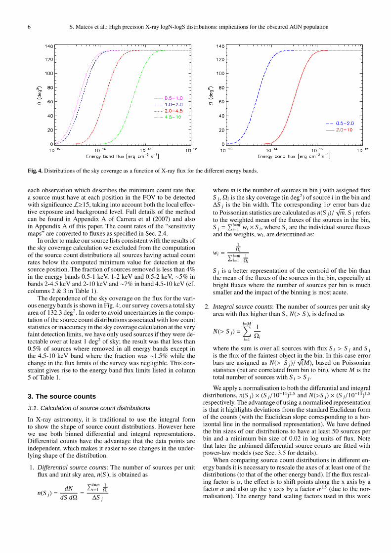
Fig. 4. Distributions of the sky coverage as a function of X-ray flux for the different energy bands.

each observation which describes the minimum count rate thata source must have at each position in the FOV to be detectedwith significanceL≥15, taking into account both the local effec-tive exposure and background level. Full details of the methodcan be found in Appendix A of Carrera et al (2007) and alsoin Appendix A of this paper. The count rates of the “sensitivitymaps” are converted to fluxes as specified in Sec. 2.4.

In order to make our source lists consistent with the results ofthe sky coverage calculation we excluded from the computationof the source count distributions all sources having actual countrates below the computed minimum value for detection at thesource position. The fraction of sources removed is less than 4%in the energy bands 0.5-1 keV, 1-2 keV and 0.5-2 keV, ∼5% inbands 2-4.5 keV and 2-10 keV and ∼7% in band 4.5-10 keV (cf.columns 2 & 3 in Table 1).

The dependence of the sky coverage on the flux for the vari-ous energy bands is shown in Fig. 4; our survey covers a total skyarea of 132.3 deg2. In order to avoid uncertainties in the compu-tation of the source count distributions associated with low countstatistics or inaccuracy in the sky coverage calculation at the veryfaint detection limits, we have only used sources if they were de-tectable over at least 1 deg2 of sky; the result was that less than0.5% of sources where removed in all energy bands except inthe 4.5-10 keV band where the fraction was ∼1.5% while thechange in the flux limits of the survey was negligible. This con-straint gives rise to the energy band flux limits listed in column5 of Table 1.

3. The source counts

3.1. Calculation of source count distributions

In X-ray astronomy, it is traditional to use the integral formto show the shape of source count distributions. However herewe use both binned differential and integral representations.Differential counts have the advantage that the data points areindependent, which makes it easier to see changes in the under-lying shape of the distribution.

1. Differential source counts: The number of sources per unitflux and unit sky area, n(S ), is obtained as

n(S j) =dN

dS dΩ=

∑i=mi=1

1Ωi

∆S j

where m is the number of sources in bin j with assigned fluxS j, Ωi is the sky coverage (in deg2) of source i in the bin and∆S j is the bin width. The corresponding 1σ error bars dueto Poissonian statistics are calculated as n(S j)/

√m. S j refers

to the weighted mean of the fluxes of the sources in the bin,S j =

∑i=mi=1 wi × S i, where S i are the individual source fluxes

and the weights, wi, are determined as:

wi =

1Ωi

∑i=mi=1

1Ωi

S j is a better representation of the centroid of the bin thanthe mean of the fluxes of the sources in the bin, especially atbright fluxes where the number of sources per bin is muchsmaller and the impact of the binning is most acute.

2. Integral source counts: The number of sources per unit skyarea with flux higher than S , N(> S ), is defined as

N(> S j) =i=M∑

i=1

1Ωi

where the sum is over all sources with flux S i > S j and S jis the flux of the faintest object in the bin. In this case errorbars are assigned as N(> S j)/

√(M), based on Poissonian

statistics (but are correlated from bin to bin), where M is thetotal number of sources with S i > S j.We apply a normalisation to both the differential and integral

distributions, n(S j) × (S j/10−14)2.5 and N(>S j) × (S j/10−14)1.5

respectively. The advantage of using a normalised representationis that it highlights deviations from the standard Euclidean formof the counts (with the Euclidean slope corresponding to a hor-izontal line in the normalised representation). We have definedthe bin sizes of our distributions to have at least 50 sources perbin and a minimum bin size of 0.02 in log units of flux. Notethat later the unbinned differential source counts are fitted withpower-law models (see Sec. 3.5 for details).

When comparing source count distributions in different en-ergy bands it is necessary to rescale the axes of at least one of thedistributions (to that of the other energy band). If the flux rescal-ing factor is α, the effect is to shift points along the x axis by afactor α and also up the y axis by a factor α1.5 (due to the nor-malisation). The energy band scaling factors used in this work


Fig. 5. Source count distributions in both a normalised differential (left) and normalised integral form (right) for sources detected in the 0.5-2keV and 2-10 keV bands. The lines show the results of the fitting of the data using a model with two (solid) and three (dashed) power-laws (seeSec. 3.5). Error bars correspond to 1σ confidence.

Table 2. Scaling factors used to convert fluxes to different energy bands.

Energy band α = S b/S 0.5−10 keV(1) (2)

0.5-1 0.151-2 0.16

2-4.5 0.294.5-10 0.390.5-2 0.322-10 0.682-8 0.562-12 0.79

4.5-7.5 0.245.0-10 0.350.5-10 1.0

(1) Energy band definition (in keV). (2) Flux scaling factor normalisedto a unit flux in the 0.5-10 keV band, where S b is the flux in the band

and S 0.5−10 keV is the flux in the 0.5-10 keV band. The values wereobtained from an unabsorbed power-law spectrum of Γ=1.9 below 2

keV and Γ=1.6 above 2 keV.

are listed in Table 2. The values are normalised to unit flux inthe 0.5-10 keV band.

Hereafter we will use the term ‘steeper’ source counts to re-fer to those distributions having a greater numerical index for theslope, while ‘flatter’ distributions will be those having smallervalues of |Γ|.

3.2. The broad band source counts

In Fig. 5 we show the differential and integral source count distri-butions derived in the ’standard’ 0.5-2 keV and 2-10 keV bands.A comparison with those obtained using data taken directly fromthe 2XMM catalogue is presented in Appendix B.

Our survey provides tight constraints on the X-ray sourcecounts over more than 2 decades of X-ray flux in both energybands. In Fig. 5 the solid and dashed lines show the results ofthe fitting to the differential source counts with a power-law withtwo and three components (see Sec. 3.5 for details). A break inthe source count distributions is obvious in both bands, althoughin the 2-10 keV band the measurements do not go deep enoughto properly define the shape of the distribution below the break.The cumulative angular density of sources in the broad energybands at different fluxes is given in Table 3.

We have compared our results with previous findingsfrom deep and shallow representative surveys (see Fig. 6).


Fig. 6. Comparison of the 0.5-2 keV (left) and 2-10 keV (right) normalised integral source count distributions (filled circles) with a set of repre-sentative results from previous surveys. Error bars correspond to 1σ confidence.

Table 3. The cumulative angular density of sources in the broad bands.

Flux N(> S) N N(> S) N0.5-2 keV 2-10 keV

(1) (2) (3) (4) (5)-14.84 605.7± 3.4∗ 31837 - --14.70 474.0± 2.7 31465 - --14.43 287.4± 1.7 27944 - --14.40 268.4± 1.6 27119 - --14.10 132.9± 1.0 16715 - --14.04 111.2± 0.9 14283 315.6± 3.2∗ 9431-13.85 65.9± 0.7 8674 181.2± 1.9 8911-13.80 57.0± 0.7 7521 155.6± 1.7 8628-13.50 21.7± 0.4 2871 54.0 ± 0.7 5443-13.20 8.0± 0.2 1057 17.0 ± 0.4 2172-12.90 3.0± 0.2 395 5.3 ± 0.2 704-12.60 1.0± 0.1 138 1.6 ± 0.1 213-12.30 0.4± 0.1 53 0.4 ± 0.1 55

(1) Energy band flux in log units. (2) Cumulative angular density ofsources in units of deg−2 above a given flux in the 0.5-2 keV energy

band. (3) Number of sources above given flux in the 0.5-2 keV energyband. (2) Cumulative angular density of sources in units of deg−2

above a given flux in the 2-10 keV energy band. (3) Number of sourcesabove given flux in the 2-10 keV energy band. ∗ Cumulative angular

density of sources at the flux limits of our survey in the 0.5-2 keV and2-10 keV bands.

In the 0.5-2 keV band, the form of the source counts be-low ∼10−14 erg cm−2 s−1 has been determined previously fromboth medium-deep XMM-Newton (ELAIS-S1: Puccetti etal. 2006, XMM-COSMOS: Cappelluti et al. 2007, An XMM-NewtonInternational Survey (AXIS): Carrera et al. 2007) and Chandrasurveys (CDF-N and CDF-S: Bauer et al. 2004, Champ: Kimet al. 2007). Fig. 6 (left) also shows the data from Hasinger etal. (2005, HMS05) which is a compilation of results from vari-ous ROSAT, XMM-Newton and Chandra surveys. In general thepresent measurements are in good agreement with the publishedresults.

At bright 0.5-2 keV fluxes, where the number of sources in-cluded in the surveys is much lower, there are still uncertaintiesin the shape of the source count distributions. We note that inthe flux range 2 × 10−14 − 2 × 10−13 erg cm−2 s−1 our distributiontends to lie above the results from the XMM-COSMOS and Champ

surveys. One important difference in our analysis (and also in theAXIS survey) is that our source count distributions include bothpoint and (modestly) extended sources, while the distributionsfrom the XMM-COSMOS and Champ surveys are for point sourcesonly. Indeed if we exclude the sources detected in our analysisas extended, then a better agreement between our results and theXMM-COSMOS survey is obtained, although the shape of the dis-tribution is still somewhat steeper than the one from the Champsurvey.

In the 2-10 keV band a detailed comparison is made moredifficult by the fact that the effective area of the X-ray detec-tors typically varies substantially across the band, which mayintroduce systematic errors in the comparison of the results fromdifferent instruments. For example, because of the low effectivearea of the X-ray detectors on-board Chandra above ∼8 keV,published Chandra results are limited to the 2-8 keV band. InAppendix B we compare the source count distributions in the 2-10 keV and 2-8 keV energy bands for our sources. There is ingeneral a good agreement between these distributions althoughthe slope of the source counts below the break is marginally flat-ter for the distribution in the 2-8 keV band. In addition the resultsfrom the XMM-COSMOS survey in the 2-10 keV band are based onsource detection in the 2-4.5 keV energy band, and hence theiranalysis could be missing a population of sources with very hardX-ray spectra. Additional discrepancies between source countsmay be explained by the different spectral assumption used intheir construction. As we explained in Sec. 2.4, this could affectthe measured normalisation of the source count distributions byup to ∼20%. Finally if we adopt a conservative 10% estimateon the absolute flux calibration of the EPIC pn camera, then a∼15% uncertainty in the normalisation of the source counts ob-tained with XMM-Newton might still be present (Stuhlinger etal. 2008).

Despite these caveats the overall agreement between mostsurveys in the 2-10 keV energy band is better than 10% atfluxes ≤ 10−13 erg cm−2 s−1. At brighter fluxes, the largest dis-crepancy is found when comparing with the results from theASCA Medium Sensitivity Survey (AMSS, Ueda et al. 2005)which has a normalisation ∼20-30% higher than ours. A highernormalisation on the ASCA source counts compared with previ-ous XMM-Newton surveys has been already reported (Cowie etal. 2002). Cross calibration effects need to be taken into account


Fig. 7. Source count distributions in both normalised differential (left) and normalised integral form (right) for sources detected in the 0.5-1 keV,1-2 keV, 2-4.5 keV and 4.5-10 keV bands. The lines show the results of the fitting of the data using a model with two (solid) and three (dashed)power-laws (see Sec. 3.5). Error bars correspond to 1σ confidence.


Table 4. Cumulative angular density of sources in the narrow energy bands.

Flux N(> S) N N(> S) N N(> S) N N(> S) N0.5-1 keV 1-2 keV 2-4.5 keV 4.5-10 keV

(1) (2) (3) (4) (5) (6) (7) (8) (9)-15.00 417.6± 2.9∗ 20694 - - - - - --14.93 363.0± 2.5 20604 470.7± 3.2∗ 21185 - - - --14.84 315.8± 2.2 20394 404.4± 2.8 21059 - - - --14.70 239.4± 1.7 19429 300.3± 2.1 20338 - - - --14.43 132.9± 1.1 14856 157.6± 1.2 16004 302.4± 3.1∗ 9564 - --14.40 122.3± 1.0 14054 144.5± 1.2 15212 272.5± 2.8 9523 - --14.10 56.1± 0.7 7291 58.2± 0.7 7452 110.6± 1.2 7980 - --14.04 46.3± 0.6 6071 47.1± 0.6 6125 89.6± 1.0 7325 - --13.85 26.5± 0.4 3501 24.9± 0.4 3286 46.8± 0.7 5022 92.2± 2.1∗ 1895-13.80 22.8± 0.4 3013 21.1± 0.4 2796 39.0± 0.6 4407 73.8± 1.7 1867-13.50 8.9± 0.3 1183 7.5± 0.2 989 12.3± 0.3 1598 22.1± 0.6 1432-13.20 3.4± 0.2 453 2.9± 0.1 380 4.0± 0.2 534 6.6± 0.2 731-12.90 1.4± 0.1 187 1.0± 0.1 134 1.3± 0.1 175 2.3± 0.1 293-12.60 0.6± 0.1 73 0.4± 0.1 55 0.5± 0.1 66 0.7± 0.1 89-12.30 0.1± 0.1 18 0.1± 0.1 16 0.1± 0.1 15 0.2± 0.1 27

(1) Energy band flux in log units. (2) Cumulative angular density of sources in units of deg−2 above given flux in the 0.5-1 keV energy band. (3)Number of sources above given flux in the 0.5-1 keV energy band. (4) Cumulative angular density of sources in units of deg−2 above given flux inthe 1-2 keV energy band. (5) Number of sources above given flux in the 1-2 keV energy band. (6) Cumulative angular density of sources in unitsof deg−2 above given flux in the 2-4.5 keV energy band. (7) Number of sources above given flux in the 2-4.5 keV energy band. (8) Cumulative

angular density of sources in units of deg−2 above given flux in the 4.5-10 keV energy band. (9) Number of sources above given flux in the 4.5-10keV energy band. ∗ Cumulative angular density of sources at the flux limit of our survey in the various narrow energy bands.

when comparing results from different missions and could ex-plain the observed discrepancies. Snowden (2002) investigatedthe cross calibration between different missions, including ASCAand XMM-Newton and found an agreement between ASCA andXMM-Newton fluxes at the ∼10% level. Since this analysis,changes in EPIC-pn 2-10 keV fluxes associated with improve-ments in the calibration have been ∼1-2%, and therefore the∼10% discrepancy between ASCA and XMM-Newton EPIC-pnstill holds. We conclude that the observed discrepancy with re-spect to ASCA source counts cannot be explained as a cross cali-bration effect alone.

We also note that the recently published source count distri-butions for sources detected by XMM-Newton in the LockmanHole field in the 0.5-2 keV and 2-10 keV energy bands arealso consistent with our results within 1 to 2-σ at fluxes≤ 10−14 erg cm−2 s−1 (Brunner et al. 2008). In order to compareour source count distributions with previous results at fluxesbrighter than those sampled by our analysis we compare withthe ROSAT All-Sky Survey data in the 0.5-2 keV band (HMS05,Fig. 6 left) and the HEAO1 A-2 all-sky survey in the 2-10 keVband for AGN-only sources (Piccinotti et al. 1982, Fig. 6 right).The extrapolation to brighter fluxes of our source counts, showsthat our distributions lie marginally below these results. This dis-crepancy can be explained as being due to the fact that surveysusing pointed observations (such as this survey) may be biasedagainst bright sources because the targets of the observationshave to be excluded from the analysis.

3.3. The narrow band source counts

If we compare the 0.5-2 keV and 2-10 keV source counts we seethat there is a strong dependence of the shape of the distributionson the energy band. A similar trend is found when we comparethe source count distributions in our narrow energy bands, 0.5-1keV, 1-2 keV, 2-4.5 keV and 4.5-10 keV (see Fig. 7): the sourcecount distributions become steeper both at faint and bright fluxesas we move to higher energies. The cumulative angular density

Fig. 8. Comparison of the measured normalised integral 4.5-10 keVsource count distribution (filled circles) with a sample of representativeresults from previous surveys. Error bars correspond to 1σ confidence.

of sources in the narrow energy bands at different fluxes is givenin Table 4.

In Fig. 8 we show the source count distribution in the high-est energy range sampled in our analysis, namely 4.5-10 keV.We also include some representative results from previous sur-veys for comparison: in the 5-10 keV band the results fromELAIS-S1 (Puccetti et al. 2006), CDF-S 1σ (Rosati et al. 2002),XMM-COSMOS (Cappelluti et al. 2007) and the XMM-Newton 13H

field (Loaring et al. 2005); in the 4.5-7.5 keV energy band theXMM-Newton Hard Bright Serendipitous Survey (HBSS, DellaCeca et al. 2004) and AXIS (Carrera et al. 2007); in the 4.5-10keV band the Beppo SAX data from Fiore et al. (2001). In orderto convert the fluxes from these surveys to the 4.5-10 keV en-ergy band we assumed that the spectra of the sources can be wellrepresented by a power-law of slope Γ=1.6. The corresponding


Table 5. Results of the maximum likelihood fits to our source countdistributions with a broken power-law model.

Energy band Γb Γf S b K(keV) (10−14 cgs) (deg−2)

(1) (2) (3) (4) (5)0.5-1 2.30+0.02

−0.01 1.78+0.01−0.02 0.81+0.01

−0.01 71.3+1.5−11.6

1-2 2.43+0.01−0.01 1.81+0.01

−0.01 0.65+0.01−0.01 112.3+2.2

−1.02-4.5 2.62+0.02

−0.02 2.24+0.04−0.03 1.46+0.15

−0.07 72.6+4.7−12.1

4.5-10a 2.69+0.03−0.03 —- —- 264.8+15.8

−14.7

0.5-2 2.31+0.01−0.01 1.66+0.01

−0.02 1.06+0.13−0.01 124.9+1.8

−18.60.5-2b 2.29+0.01

−0.55 1.63+0.01−0.33 1.00+0.01

−0.01 131.9+1.1−45.5

2-10 2.65+0.02−0.02 2.30+0.05

−0.03 3.29+0.15−0.08 84.4+3.3

−6.12-10a 2.54+0.01

−0.01 —- —- 482.6+10.8−9.2

2-10b 2.55+0.03−0.02 1.19+0.01

−0.01 0.78+0.01−0.10 709.3+110.6

−18.0

(1) Energy band definition (in keV). (2) Power-law slope above theflux break. (3) Power-law slope below the flux break. (4) and (5) Fluxbreak (in units of 10−14 erg cm−2 s−1) and normalisation in each band.Errors are 1σ uncertainty. a Best fit parameters from using a single

power-law. b Best fit parameters from fitting our data together with thedata from the CDF-N and CDF-S.

factors used to convert fluxes to the 4.5-10 keV energy band arelisted in Table 2.

At energies &4.5 keV there is still a lack of strong obser-vational constraints in the shape of the source count distribu-tion, as large discrepancies in the results for both the shape andnormalisation of the distribution are evident. In some cases thisamounts to >30%. Because the effective area of the X-ray detec-tors at these energies is relatively small, the number of sourcesinvolved in these analyses is correspondingly limited. In addi-tion, a ∼10-20% uncertainty in the normalisation can arise dueto the uncertainty in the absolute flux calibration of the instru-ments and the spectral shape chosen in the count rate to flux con-version (see Sec. 2.4). The latter, however, cannot fully explainthe observed discrepancies in the results as most of the surveyscompute their fluxes using the same spectral index. We note thatthe measurements of Beppo SAX (Fiore et al. 2001) are sys-tematically higher than the results based on XMM-Newton data.The disagreement with the Beppo SAX results was already notedby Della Ceca et al. (2004), who suggested that an offset in theBeppo SAX absolute flux calibration of ∼30% could explain thediscrepancy in the results.

Thanks to our study we can now constrain the shape andnormalisation of the source counts above 4.5 keV over areasonably broad range of flux, from ∼ 10−14 erg cm−2 s−1 to∼ 3 × 10−13 erg cm−2 s−1. Note that in the 4.5-10 keV band nobreak in the source count distribution is detected down to thelimiting flux of our survey, ∼1.4 × 10−14 erg cm−2 s−1. This isconsistent with the results from deeper X-ray surveys whichsuggest that the break in the source counts at energies above∼4.5 keV must occur at fluxes .5-8×10−15 erg cm−2 s−1 (seee.g. Loaring et al. 2005, Brunner et al. 2008, Georgakakis etal. 2008).

3.4. Confusion, bias and other systematic effects in sourcecounts

We have not corrected our source count distributions for bi-ases associated with the source detection procedure such asEddington bias, source confusion or spurious detections. It is

10-14 10-13

S4.5-10 keV

[erg cm-2 s-1]

100

N(>

S)

S1.

5

14 [d

eg-2]

Alltexp

>50 ks30 ks<t

exp<50 ks

12 ks<texp

<30 kstexp

<12 ks

L>10 L>15 L>30 L>50

Fig. 9. Top: Dependence of the 4.5-10 keV normalised source countdistribution in integral form on the exposure time of the observations.Bottom: Comparison of our 4.5-10 keV normalised source count dis-tribution in integral form (L≥15) with the distributions obtained iflower/higher detection likelihood thresholds are used instead. Error barscorrespond to 1σ confidence.

therefore important to quantify the potential effect of these bi-ases on our results.

First we note that there is excellent agreement betweenour results and previous surveys which have gone substantiallydeeper and hence are less susceptible to bias effects at fluxthresholds relevant to the current survey (e.g. Bauer et al. 2004,Cappelluti et al. 2007). This suggests that our source count dis-tributions are not strongly affected by source detection biases.

Source confusion occurs when two or more sources fall ina single resolution element of the detector, and depends on thesky density of sources and the size of the telescope beam. Asshown in Loaring et al. (2005), the XMM-Newton confusionlimit is reached at a source density of ∼2000 deg−2, correspond-ing to fluxes < 10−16 erg cm−2 s−1 in all energy bands. This iswell below the flux limits reached by our survey (see Table 1).Therefore we expect the effect of source confusion on our sourcecount distributions to be negligible. Furthermore, due to the rel-atively high threshold in detection likelihood used in our analy-sis (L≥15), we expect the fraction of spurious detections in oursamples to be low. From Fig. 6 in Loaring et al. (2005), a detec-tion likelihood L=10 corresponds to a ∼2.6% fraction of spuri-


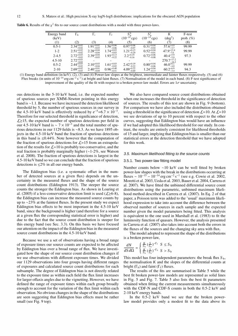
Table 6. Results of the χ2 fits to our source count distributions with a model with three power-laws.

Energy band Γb Γi Γf S bb S f

b K F-test(keV) (10−14 cgs) (10−14 cgs) (deg2) prob. (%)

(1) (2) (3) (4) (5) (6) (7) (8)0.5-1 2.34+0.02

−0.02 1.91+0.02−0.03 1.56+0.06

−0.06 0.97+0.06−0.07 0.31+0.04

−0.02 57.6+4.9−3.7 99.99

1-2 2.51+0.02−0.02 2.28+0.04

−0.04 1.74+0.03−0.03 1.21+0.15

−0.20 0.52+0.04−0.01 47.9+12.4

−7.6 99.992-4.5 2.72+0.03

−0.03 2.39+0.04−0.03 1.93+0.13

−0.22 2.2+0.19−0.16 0.72+0.06

−0.08 40.4+5.9−5.9 97.3

4.5-10 2.72+0.03−0.03 - - - - 270.7+17.2

−16.20.5-2 2.44+0.03

−0.02 2.10+0.03−0.04 1.61+0.03

−0.02 2.42+0.19−0.22 0.80+0.04

−0.06 46.0+6.1−4.0 99.99

2-10 2.69+0.02−0.03 2.40+0.01

−0.04 0.96+0.40−0.51 4.09+0.22

−0.69 1.24+0.04−0.13 60.2+6.9

−3.4 94.3(1) Energy band definition (in keV). (2), (3) and (4) Power-law slopes at the brightest, intermediate and fainter fluxes respectively. (5) and (6)Flux breaks (in units of 10−14 erg cm−2 s−1) at bright and faint fluxes. (7) Normalisation of the model in each band. (8) F-test significance of

improvement of the quality of the fit with respect to a broken power-law model. Errors are 1σ uncertainty.

ous detections in the 5-10 keV band, i.e. the expected numberof spurious sources per XMM-Newton pointing in this energyband is ∼1.1. Because we have increased the detection likelihoodthreshold by 5, the number of spurious sources in our survey inthe 4.5-10 keV band is effectively reduced by e−5=6.7 × 10−3.Therefore for our selected threshold in significance of detection,L≥15, the expected number of spurious detections per field inour 4.5-10 keV band is ∼ 7 × 10−3 and the total number of spu-rious detections in our 1129 fields is ∼8.3. As we have 1895 ob-jects in the 4.5-10 keV band the fraction of spurious detectionsin this band is ≤0.44%. Note however that the computation ofthe fraction of spurious detections for L=15 from an extrapola-tion of the results forL=10 is probably too conservative, and thereal fraction is probably marginally higher (∼1-2%, see Watsonet al. 2008). The fraction of spurious detections is largest in the4.5-10 keV band so we can conclude that the fraction of spuriousdetections is .2% in all our energy bands.

The Eddington bias (i.e. a systematic offset in the num-ber of detected sources at a given flux) depends on the un-certainty in the measured fluxes and the shape of the sourcecount distributions (Eddington 1913). The steeper the sourcecounts the stronger the Eddington bias. As shown in Loaring etal. (2005) if a less-conservative detection limit is used (L≥6-8),the Eddington bias can increase the measured source counts byup to ∼23% at the faintest fluxes. In the present study we expectEddington bias effects to be most important in the 4.5-10 keVband, since the background is higher (and therefore for a sourceat a given flux the corresponding statistical error is higher) anddue to the fact that the source count distribution is steeper forthis energy band (see Sec. 3.3). On this basis we have focusedour attention on the impact of the Eddington bias in the measuredsource count distributions in the 4.5-10 keV band.

Because we use a set of observations having a broad rangeof exposure times our source counts are expected to be affectedby Eddington bias over a broad range of flux. We have investi-gated how the shape of our source count distribution changes ifwe use observations with different exposure times. We dividedour 1129 observations into four groups having different rangesof exposures and calculated source count distributions for eachsubsample. The degree of Eddington bias is not directly relatedto the exposure time as within each field the flux limit increasesfor larger offaxis angles due to the vignetting. However, we havedefined the range of exposure times within each group broadlyenough to account for the variation of the flux limit within eachobservation. No obvious changes in the shape of the distributionsare seen suggesting that Eddington bias effects must be rathersmall (see Fig. 9 top).

We also have compared source count distributions obtainedwhen one increases the threshold in the significance of detectionof sources. The results of this test are shown in Fig. 9 (bottom).For comparison we have also included the distribution obtainedusing a threshold in the significance of detectionL=10. AtL=10we see deviations of up to 10 percent with respect to the othercurves, suggesting that Eddington bias would have an influenceif we had adopted this likelihood threshold for our study. In con-trast, the results are entirely consistent for likelihood thresholdsof 15 and larger, implying that Eddington bias is smaller than ourstatistical errors at the detection threshold that we have adoptedfor this work.

3.5. Maximum likelihood fitting to the source counts

3.5.1. Two power-law fitting model

Number counts below ∼10 keV can be well fitted by brokenpower-law shapes with the break in the distributions occurring atfluxes ∼ 10−15 − 10−14 erg cm−2 s−1 (see e.g. Cowie et al. 2002,Moretti et al. 2003, Ueda et al. 2003, Bauer et al. 2004, Carrera etal. 2007). We have fitted the unbinned differential source countdistributions using the parametric, unbinned maximum likeli-hood method described in Carrera et al. (2007). In Eq. 2 of thatpaper, a Poisson term was added to the ’usual’ maximum likeli-hood expression to take into account the difference between theobserved number of sources in each sample and the expectednumber given the model parameters being fitted. This analysisis equivalent to the one used in Marshall et al. (1983) to fit theluminosity function of quasars. However, the analysis presentedin Carrera et al. (2007) also takes into account both the errors inthe fluxes of the sources and the changing sky area with flux.

The model adopted to represent the shape of the distributionsis a broken power-law,

dNdS dΩ

=

KS b

( SS b

)−Γf S ≤ S bKS b

( SS b

)−Γb S > S b

This model has four independent parameters: the break flux S b,the normalisation K and the slopes of the differential counts atbright (Γb) and faint (Γf) fluxes.

The results of the fits are summarised in Table 5 while thebest fit broken power-law models are represented as solid linesin Fig. 5 and Fig. 7. Table 5 also lists the best fit parametersobtained when fitting the current measurements simultaneouslywith the CDF-N and CDF-S counts in both the 0.5-2 keV and2-10 keV energy bands.

In the 0.5-2 keV band we see that the broken power-law model provides only a modest fit to the data above its


Table 7. Intensity of the X-ray background contributed by our sources in the various energy bands.

Energy band S min S max ICXRB(S min ≤ S ≤ S max) ICXRB fCXRB(keV) (cgs) (cgs) (10−12cgs deg−2) (10−12cgs deg−2)

(1) (2) (3) (4) (5) (6)0.5-1 9.9 × 10−16 10−12 2.4 2.96 0.81

10−12 0.32 0.111-2 1.2 × 10−15 10−12 2.5 4.50* 0.55

10−12 0.12 0.032-4.5 3.7 × 10−15 10−12 3.3 7.80 0.42

10−12 0.08 0.014.5-10 14 × 10−15 10−12 2.8 12.4 0.22

10−12 0.14 0.01

0.5-2 1.4 × 10−15 10−12 4.9 7.50* 0.6510−12 0.48 0.06

2-10 9.0 × 10−15 10−12 8.0 20.2* 0.3910−12 0.39 0.02

(1) Energy band definition (in keV). (2) and (3) Minimum and maximum flux used in the integration. (4) Intensity of the X-ray backgroundcontributed by our sources. Note that the quoted values include the contribution from both clusters of galaxies and stars. (5) Total X-ray

background intensity. Errors are 1σ uncertainty. The values indicated with an asterisk are from Moretti et al. (2003). These values were used toestimate the CXRB intensity in the various energy bands assuming a power-law model of Γ=1.4 (see Sec. 3.6 for details). (6) Fraction of X-ray

background resolved by our sources.

break suggesting that the curvature of the source counts inthe 0.5-2 keV band cannot be well represented by a simplebroken power-law model. Although in the 2-10 keV band themodel seems to provide a better representation of the shape ofthe source counts, this is only achieved by allowing a breakat a flux > 3 × 10−14 erg cm−2 s−1, well above the value of∼ 10−14 erg cm−2 s−1 typically found in deeper surveys (see e.g.Cappelluti et al. 2007). We interpret this as an indication thatthe curvature of the source counts also in the 2-10 keV bandcannot be well reproduced by the broken power-law model. Forthe narrow energy bands the broken power-law model provides asomewhat better although far from perfect fit to all the data sets(see Fig. 7).

3.5.2. Three power-law fitting model

In order to improve the quality of the fits to our source countswe performed a χ2 fitting to the binned differential distributionsusing a model with three power-law components. This modelhas six independent parameters: the break fluxes at bright andfaint fluxes, S b

b and S fb; the normalisation K at the bright flux

break and the slopes at bright (Γb), intermediate (Γi) and faint(Γf) fluxes. A summary of the results of the fitting are given inTable 6. Column 8 lists the F-test significance of improvementof the fits relative to a model with two power-laws.

The results for the 0.5-1 keV, 1-2 keV and 0.5-2 keV spectralregimes confirm that the curvature of the source counts in theseenergy bands cannot be well reproduced with the standard bro-ken power-law model. The same result probably applies also tothe source counts in the 2-4.5 keV and 2-10 keV energy bands,although in this case the lower significance of improvement inthe fits is probably due to the fact that our survey is not deepenough at these energies to provide strong constraints on theshape of the distributions below the region of downward cur-vature in the counts.

3.6. Contribution to the cosmic X-ray background

We have used the best fit parameters of our source count dis-tributions (three power-law model, see Table 6) to estimate theintensity contributed by our sources to the cosmic X-ray back-ground in the various energy bands. The results are presentedin Table 7. Here we use the CXRB intensity measurements ob-tained by Moretti et al. (2003) in the 1-2 keV and 2-10 keVbands, which are consistent within 1σwith the more recent mea-surements of the X-ray background intensity obtained by DeLuca & Molendi (2004) and Hickox & Markevitch (2006). Inorder to compute the values in our energy bands we assumeda spectral model with power-law Γ=1.4, which is known to bean appropriate representation of the CXRB spectrum at ener-gies above 2 keV (Lumb et al. 2002). The shape of the CXRBspectrum at energies below ∼1 keV is rather uncertain althoughsource stacking analyses suggest a marginally softer spectrum(e.g. Streblyanska et al. 2004). We decided to use the same valueof Γ down to 0.5 keV and therefore the value of the CXRB in-tensity in the 0.5-1 keV band reported in Table 7 could be po-tentially underestimated. In Table 7 we also list the values ofthe CXRB intensity contributed by sources with fluxes above10−12 erg cm−2 s−1. These values were obtained by integratingthe best fit model of our source count distributions. We estimatethat the uncertainty in the values reported in Table 7 is dominatedby systematics (e.g. those associated with spectral assumptions,flux conversions and instrumental calibrations), i.e. not sourcestatistics, and therefore uncertainties in our measurements of theCXRB intensity should be . 5%.

The source count distributions obtained by Moretti etal. (2003) in the 0.5-2 keV and 2-10 keV energy bands have beenfrequently used to estimate the contribution from bright sourcesto the X-ray background (e.g. Worsley et al. 2004, Worsley etal. 2005). However, it has already been pointed out that theMoretti et al. (2003) bright end slopes might be too steep sug-gesting that bright-end corrections for the CXRB intensity couldbe an underestimate (see Worlsley et al. 2005). We also foundthat the bright end slope of our source counts is flatter than thevalue reported in Moretti et al. (2003) (2.82+0.07

−0.09). However inthe 2-10 keV band our bright end slope is marginally flatter al-


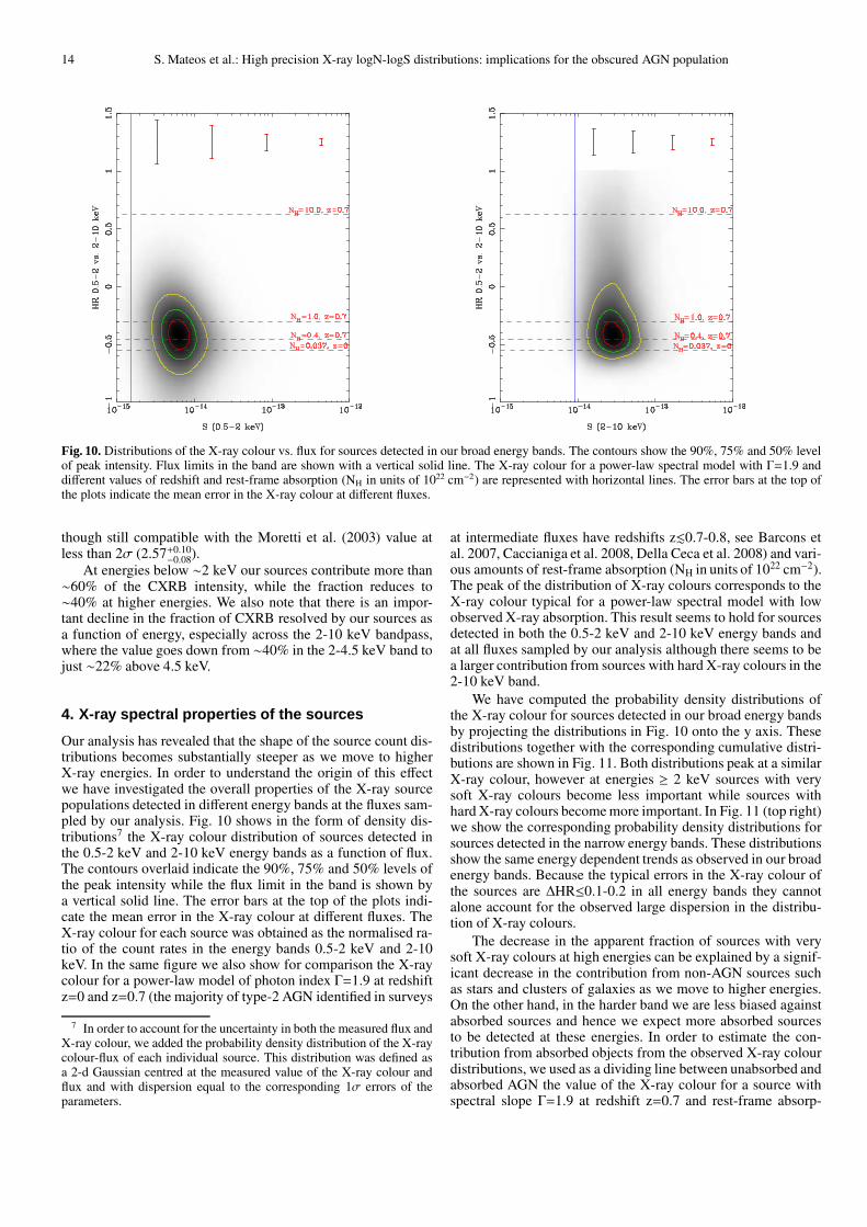
Fig. 10. Distributions of the X-ray colour vs. flux for sources detected in our broad energy bands. The contours show the 90%, 75% and 50% levelof peak intensity. Flux limits in the band are shown with a vertical solid line. The X-ray colour for a power-law spectral model with Γ=1.9 anddifferent values of redshift and rest-frame absorption (NH in units of 1022 cm−2) are represented with horizontal lines. The error bars at the top ofthe plots indicate the mean error in the X-ray colour at different fluxes.

though still compatible with the Moretti et al. (2003) value atless than 2σ (2.57+0.10

−0.08).At energies below ∼2 keV our sources contribute more than

∼60% of the CXRB intensity, while the fraction reduces to∼40% at higher energies. We also note that there is an impor-tant decline in the fraction of CXRB resolved by our sources asa function of energy, especially across the 2-10 keV bandpass,where the value goes down from ∼40% in the 2-4.5 keV band tojust ∼22% above 4.5 keV.

4. X-ray spectral properties of the sources

Our analysis has revealed that the shape of the source count dis-tributions becomes substantially steeper as we move to higherX-ray energies. In order to understand the origin of this effectwe have investigated the overall properties of the X-ray sourcepopulations detected in different energy bands at the fluxes sam-pled by our analysis. Fig. 10 shows in the form of density dis-tributions7 the X-ray colour distribution of sources detected inthe 0.5-2 keV and 2-10 keV energy bands as a function of flux.The contours overlaid indicate the 90%, 75% and 50% levels ofthe peak intensity while the flux limit in the band is shown bya vertical solid line. The error bars at the top of the plots indi-cate the mean error in the X-ray colour at different fluxes. TheX-ray colour for each source was obtained as the normalised ra-tio of the count rates in the energy bands 0.5-2 keV and 2-10keV. In the same figure we also show for comparison the X-raycolour for a power-law model of photon index Γ=1.9 at redshiftz=0 and z=0.7 (the majority of type-2 AGN identified in surveys

7 In order to account for the uncertainty in both the measured flux andX-ray colour, we added the probability density distribution of the X-raycolour-flux of each individual source. This distribution was defined asa 2-d Gaussian centred at the measured value of the X-ray colour andflux and with dispersion equal to the corresponding 1σ errors of theparameters.

at intermediate fluxes have redshifts z.0.7-0.8, see Barcons etal. 2007, Caccianiga et al. 2008, Della Ceca et al. 2008) and vari-ous amounts of rest-frame absorption (NH in units of 1022 cm−2).The peak of the distribution of X-ray colours corresponds to theX-ray colour typical for a power-law spectral model with lowobserved X-ray absorption. This result seems to hold for sourcesdetected in both the 0.5-2 keV and 2-10 keV energy bands andat all fluxes sampled by our analysis although there seems to bea larger contribution from sources with hard X-ray colours in the2-10 keV band.

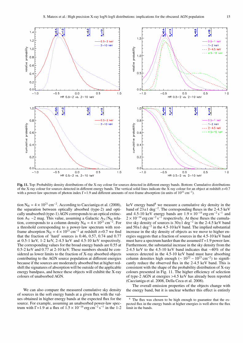
We have computed the probability density distributions ofthe X-ray colour for sources detected in our broad energy bandsby projecting the distributions in Fig. 10 onto the y axis. Thesedistributions together with the corresponding cumulative distri-butions are shown in Fig. 11. Both distributions peak at a similarX-ray colour, however at energies ≥ 2 keV sources with verysoft X-ray colours become less important while sources withhard X-ray colours become more important. In Fig. 11 (top right)we show the corresponding probability density distributions forsources detected in the narrow energy bands. These distributionsshow the same energy dependent trends as observed in our broadenergy bands. Because the typical errors in the X-ray colour ofthe sources are ∆HR≤0.1-0.2 in all energy bands they cannotalone account for the observed large dispersion in the distribu-tion of X-ray colours.

The decrease in the apparent fraction of sources with verysoft X-ray colours at high energies can be explained by a signif-icant decrease in the contribution from non-AGN sources suchas stars and clusters of galaxies as we move to higher energies.On the other hand, in the harder band we are less biased againstabsorbed sources and hence we expect more absorbed sourcesto be detected at these energies. In order to estimate the con-tribution from absorbed objects from the observed X-ray colourdistributions, we used as a dividing line between unabsorbed andabsorbed AGN the value of the X-ray colour for a source withspectral slope Γ=1.9 at redshift z=0.7 and rest-frame absorp-


Fig. 11. Top: Probability density distributions of the X-ray colour for sources detected in different energy bands. Bottom: Cumulative distributionsof the X-ray colour for sources detected in different energy bands. The vertical solid lines indicate the X-ray colour for an object at redshift z=0.7with a power-law spectrum of photon index Γ=1.9 and different amounts of rest-frame absorption (in units of 1022 cm−2).

tion NH = 4 × 1021 cm−2. According to Caccianiga et al. (2008),the separation between optically absorbed (type-2) and opti-cally unabsorbed (type-1) AGN corresponds to an optical extinc-tion AV ∼2 mag. This value, assuming a Galactic AV/NH rela-tion, corresponds to a column density NH = 4 × 1021 cm−2. Fora threshold corresponding to a power-law spectrum with rest-frame absorption NH = 4 × 1021 cm−2 at redshift z=0.7 we findthat the fraction of ’hard’ sources is 0.46, 0.57, 0.74 and 0.77at 0.5-1 keV, 1-2 keV, 2-4.5 keV and 4.5-10 keV respectively.The corresponding values for the broad energy bands are 0.55 at0.5-2 keV and 0.77 at 2-10 keV. These numbers should be con-sidered as lower limits to the fraction of X-ray absorbed objectscontributing to the AGN source population at different energiesbecause if the sources are moderately absorbed but at higher red-shift the signatures of absorption will be outside of the applicableenergy bandpass, and hence these objects will exhibit the X-raycolours of unabsorbed AGN.

We can also compare the measured cumulative sky densityof sources in the soft energy bands at a given flux with the val-ues obtained in higher energy bands at the expected flux for thesource. For example, assuming an unabsorbed power-law spec-trum with Γ=1.9 at a flux of 1.5 × 10−14 erg cm−2 s−1 in the 1-2

keV energy band8 we measure a cumulative sky density in theband of 23±1 deg−2. The corresponding fluxes in the 2-4.5 keVand 4.5-10 keV energy bands are 1.9 × 10−14 erg cm−2 s−1 and2 × 10−14 erg cm−2 s−1 respectively. At these fluxes the cumula-tive sky density of sources is 30±1 deg−2 in the 2-4.5 keV bandand 50±1 deg−2 in the 4.5-10 keV band. The implied substantialincrease in the sky density of objects as we move to higher en-ergies suggests that a fraction of sources in the 4.5-10 keV bandmust have a spectrum harder than the assumed Γ=1.9 power-law.Furthermore, the substantial increase in the sky density from the2-4.5 keV to the 4.5-10 keV band indicates that ∼40% of thesources detected in the 4.5-10 keV band must have absorbingcolumn densities high enough (∼ 1022 − 1023 cm−2) to signifi-cantly reduce the observed flux in the 2-4.5 keV band. This isconsistent with the shape of the probability distribution of X-raycolours presented in Fig. 11. The higher efficiency of selectionof type-2 AGN at energies >4.5 keV has already been reported(Caccianiga et al. 2008, Della Ceca et al. 2008).

The overall emission properties of the objects change withthe energy band, but it is unclear whether this effect is entirely

8 The flux was chosen to be high enough to guarantee that the ex-pected flux in the energy bands at higher energies is well above the fluxlimit in the bands.


Fig. 12. Normalised source count distribution in integral form for starsin the 0.5-2 keV band from two XMM-Newton serendipitous sur-veys at high galactic latitudes (|b| >20): the XMM-Newton MediumSensitivity Survey (XMS, circles) and the XMM-Newton bright survey(XBS, squares). The dashed line shows the best fit to the 0.5-2 keVsource count distribution for clusters from Rosati et al. (1998). Errorbars correspond to 1σ confidence.

due to the fact that we are sampling a different spectral rangeat different energies or we are detecting an intrinsically differ-ent population of sources as we move to higher energies. Thefraction of non-AGN sources decreases as we move to higherenergies. This has an effect on both the distribution of the X-ray colours, as shown previously and, as we will see in Sec. 5.2,on the shape of the source count distributions. At energies ≥2keV we find that ∼5% of the sources detected in the 4.5-10 keVband were not detected in the 2-4.5 keV band, however the ma-jority of 4.5-10 keV sources were detected both in the 2-10 keV(≥99%) and 0.5-2 keV (≥88%) energy bands. Thus, we do nothave any strong evidence that highly absorbed AGN with no softflux dominate the source counts in the harder energy bands. Thechanges in both the overall emission properties of the objectsand the shape of the source counts at different energies are bestexplained by the varying mix of the population of objects at dif-ferent fluxes and energies and the different sampling of the spec-tra of AGN. The dependence of the contribution from differentpopulations of objects to the CXRB on the energy band was al-ready noticed by Bauer et al. (2004). However their analysis wasbased on relatively broad X-ray energy bands (0.5-2 keV and 2-8 keV). The use of narrower bands has allowed us to investigatethe varying mix of different populations of objects and the rela-tive contribution from absorbed and unabsorbed AGN through-out these bandpasses and to extend the study to higher energies(10 keV).

Although the overall emission properties of the objects inthe 2-4.5 keV and 4.5-10 keV energy bands have changed sub-stantially due to the strong increase in the fraction of absorbedobjects at the highest energies, the slope of the source count dis-tributions in these energy bands has not varied significantly, in-dicating that the cosmological evolution of the sources detectedin the two energy bands must be quite similar.

5. Implications for CXRB synthesis models

5.1. The contribution of stars and clusters

Before comparing our source counts in different energy bandswith the predictions from current CXRB synthesis models weneed to account first for the contribution from non-AGN to oursamples of X-ray sources. The two most important contributorsare clusters of galaxies and stars, especially at bright fluxes andsoft X-ray energies.

1. Source counts for clusters: In order to account for clustercontribution, we have used the 0.5-2 keV source count dis-tribution for clusters from Rosati et al. (1998), that covers theflux range from ∼ 10−14 erg cm−2 s−1 to ∼ 10−12 erg cm−2 s−1

(see Fig. 12). We have checked whether our source detec-tion algorithm is able to detect all clusters at these fluxes(either as point like or extended). In order to do that wecross-correlated our sample of objects detected in the 0.5-2 keV band with the 50 clusters from the XMM-COSMOSsurvey (Finoguenov et al. 2007) that lie in the area cov-ered by our survey. We found that 18 of their clustershave been detected in our 0.5-2 keV band, 8 as extendedand 10 as point like sources. We detected all XMM-COSMOSclusters with 0.5-2 keV fluxes ≥ 10−14 erg cm−2 s−1 (5 aspoint like sources and 8 as extended sources), while only∼13% XMM-COSMOS clusters with 0.5-2 keV fluxes below∼ 10−14 erg cm−2 s−1 are in our sample (all detected as pointlike objects). Although the numbers involved are very small,this test demonstrates that the assumption that all clusterswith fluxes ∼ 10−14 erg cm−2 s−1 are included in our samplesis reasonable.We also need to estimate the contribution of clusters to the0.5-1 keV and 1-2 keV energy bands (the contribution fromclusters at energies ≥2 keV is negligible). Assuming that allclusters are also detected in these bands we have rescaled the0.5-2 keV distribution to estimate the contribution to thesebands. In order to convert the fluxes we have assumed thatthe mean spectrum of clusters can be well represented by athermal spectrum with temperature=3 keV, abundance=1/3and redshift=0.2 (apecmodel in Xspec, Arnaud 1996)9.

2. Source counts for stars: We have calculated source countdistributions for stars using the data from two XMM-Newton serendipitous surveys at high galactic latitudes (|b| >20): the XMM-Newton Medium Sensitivity Survey (XMS;Barcons et al. 2007) and the XMM-Newton Bright Survey(XBS; Della Ceca et al. 2004, Caccianiga et al. 2008). TheXMS survey covers a total sky area of 3.33 deg2 and it hasspectroscopically identified all stars in the sample (15 ob-jects) down to a 0.5-2 keV flux ∼ 1.5 × 10−14 erg cm−2 s−1.

9 From the bolometric luminosity-temperature relation, a clusterwith a temperature ∼3 keV has a luminosity ∼ 1043 erg s−1. If thecluster is at a redshift of 0.2 the expected observed flux will be∼ 3 × 10−14 erg cm−2 s−1, i.e. in the range of fluxes sampled by oursurvey. From the cluster luminosity function objects with very hightemperature (∼10 keV) are relatively rare, while for a flux limitedsurvey the volume sampled for less luminous clusters (hence withlow temperatures) is small. This implies that flux limited surveysare expected to be dominated by clusters with typical luminosities∼ 1043 − 1044 erg s−1 (i.e. with temperatures ∼3-4 keV). More luminousclusters (∼ 1045 erg s−1) will be relatively rare, and, at the flux level sam-pled by our survey, they will be at high redshift (z∼1) and hence theywill exhibit X-ray spectra very similar to the more common, less lumi-nous objects (Henry et al. 1991).


Fig. 13. Comparison of the normalised source count distributions in integral form in the 0.5-1 keV, 1-2 keV, 2-4.5 keV and 4.5-10 keV bandswith the predictions from the synthesis models of the CXRB of Treister & Urry (2006) and Gilli et al. (2007): AGN only (solid lines),AGN+clusters+stars (dashed lines). Error bars correspond to 1σ confidence.

On the other hand the XBS covers a total sky area of 28.1 deg2

and has a complete sample of stars (49) down to a 0.5-4.5keV flux ∼ 7 × 10−14 erg cm−2 s−1. Stars at the fluxes sam-pled by our analysis have mainly low temperature thermalspectra (see e.g. Della Ceca et al. 2004, Lopez-Santiago etal. 2007). Therefore 0.5-2 keV fluxes were scaled to our var-ious energy bands assuming a thermal model with a temper-ature of 0.7 keV. The 0.5-2 keV source count distributionsfor XMS and XBS stars are shown in Fig. 12.The contribution of stars to the 2-4.5 keV and 2-10 keVenergy bands at high galactic latitudes is much less certainbecause of the lack of data at these energies. According tothe XBS survey, the cumulative sky density of stars in theabove bands at a flux of 10−13 erg cm−2 s−1 (where the sur-vey is complete) is 0.21±0.09 deg−2. We have used this valueto estimate the effect of stars on the observed source countdistributions in the two hard energy bands at bright fluxes(see Sec. 5.2). Because stars have a thermal soft spectrumtheir contribution to our source counts should decrease sig-nificantly as we move to higher energies and above ∼4.5keV their contribution is negligible (Barcons et al. 2007,Caccianiga et al. 2008).

5.2. Comparison with CXRB synthesis models

In principle synthesis models of the CXRB incorporate all theavailable information about the mean spectral properties andcosmological evolution of the sources. Therefore a comparisonof our observational constraints with their predictions can giveus some insight into the origin of the observed trends in thesource count distributions. Conversely, any deviation of the mea-surements from the predictions, might indicate the need for re-finement of the model assumptions.

We have compared our data with the predictions fromthe synthesis models of Treister & Urry (2006) and Gilli etal. (2007). These models have different recipes for the X-rayluminosity function and assume somewhat different distribu-tions of X-ray absorption. One fundamental ingredient of thesemodels, is the fraction of obscured AGN, F, its evolution andits dependence on luminosity. In the Treister & Urry (2006)model, F ∝ (1 + z)0.4, and its dependence on the X-ray lu-minosity is linear, from 100% at LX = 1042 erg s−1 to 0% atLX = 3 × 1046 erg s−1. On the other hand, in the Gilli et al. (2007)model no evolution of F is assumed and the dependence of F onthe luminosity is much flatter than in the Treister & Urry (2006)model. The significantly different assumption, relating to the in-trinsic absorption properties of AGN inherent in the two models


Fig. 14. Comparison of the normalised source count distributions in integral form in the 0.5-2 keV and 2-10 keV bands with the predictions fromthe synthesis models of the CXRB of Treister & Urry (2006) and Gilli et al. (2007): AGN only (solid lines), AGN+clusters+stars (dashed lines).Error bars correspond to 1σ confidence.

would suggest that the predictions of the two models might dif-fer, especially at low energies where the results are more affectedby X-ray absorption effects. We see in Fig. 13 that the predictedsource counts from the two models are very similar above 4.5keV, especially at the fluxes sampled by our survey. Differencesbetween the two model predictions become more clear as wemove to lower energies. The two most important differences are:

1. At bright fluxes the Treister & Urry (2006) model predicts alarger number density of AGN than the Gilli et al. (2007)model. The effect becomes more important at low ener-gies. For example, at ∼ 10−13 erg cm−2 s−1 the Treister &Urry (2006) model predicts 25-35% more AGN (dependingon the energy band) than the Gilli et al. (2007) model.

2. At all fluxes the slope of the source counts is flatter in theTreister & Urry (2006) model than in the Gilli et al. (2007)model (in the sense that the implied value of |Γ| is lower).

The comparison of our measured source count distributionswith the predictions from the two models is shown in Fig. 13 andFig. 14. We show both the AGN-only predictions from the mod-els (solid lines) and the predictions after adding to the AGN-onlysource counts (in the 0.5-1 keV, 1-2 keV and 0.5-2 keV bands)the contribution from non-AGN sources (clusters of galaxies andstars) as explained in Sec. 5.1.

At energies below 2 keV and at bright fluxes(> 10−14 erg cm−2 s−1) the measured source count distribu-tions lie significantly above model predictions for AGN-only.This appears to be due to the fact that at these energies thecontribution from non-AGN sources, mainly stars and clustersof galaxies, is not negligible. We estimated that the contributionfrom stars and clusters to the X-ray source population increasesfrom ∼13-22% at fluxes ≥ 10−14 erg cm−2 s−1 to ∼44-54% atfluxes ≥ 10−13 erg cm−2 s−1 in the 0.5-2 keV band (the exactvalue depending on the CXRB model used to calculate thefractions). The net effect of stars and clusters on the shape ofthe source counts is that the bright slopes of the distributionsare substantially flatter compared with the expectations fromthe models for AGN-only sources. Once we include the con-tribution from stars and clusters the predictions of the modelsare in better agreement with our results, although both modelsseem to overpredict the observed source counts by 20-30%

at the brightest fluxes sampled by our survey (although withthe caveat that the exact contribution of stars and clusters ofgalaxies has some uncertainty). Below 2 keV and at faint fluxes(< 10−14 erg cm−2 s−1) both models overpredict the sourcecounts. The effect is more important from the comparison withthe Gilli et al. (2007) model, resulting in a discrepancy of thedata with the model predictions ∼10-20%.

In the 2-4.5 keV band and at bright fluxes the Gilli etal. (2007) model seems to underpredict the source counts. Wehave estimated the contribution from stars in this energy bandat bright fluxes using the results from the XBS survey as spec-ified in Sec. 5.1 (0.21 ± 0.09 deg−2 at 10−13 erg cm−2 s−1). Wefind that the net effect of stars is to increase the source countsat 10−13 erg cm−2 s−1 by ∼11% with respect to the AGN-onlydistributions, obtaining a much better agreement of the modelpredictions with our data. On the other hand, at faint fluxes wefind that both models overpredict the 2-4.5 keV source counts by10-20%, as we found from the comparison of the source countsat energies below 2 keV.

In the 2-10 keV and 4.5-10 keV energy bands the agree-ment of our data with the predictions from the models forAGN-only is better than 10%. Only in the 4.5-10 keV band dothe model predictions seem to slightly underpredict our sourcecounts at the faintest fluxes sampled by our analysis. This ef-fect could be explained if the break in the source counts in thisenergy band is located at lower fluxes than those predicted bythe synthesis models as suggested from deeper X-ray surveys(.5-8×10−15 erg cm−2 s−1, e.g. Loaring et al. 2005, Brunner etal. 2008, Georgakakis et al. 2008). The effect of stars on thesource counts in these energy bands is negligible.

We find that the CXRB models overpredict by 10-20% thesource counts at energies below 4.5 keV and at faint fluxes. It isimportant to note that the models have been tuned to be in agree-ment with the Chandra Deep Field source counts at faint fluxes,but these appear to be only marginally higher (.10%) than thoseestimated by our analysis. The results of the comparison suggestthat the synthesis models might be overpredicting the numberof faint absorbed AGN as has been reported in the past by pre-vious surveys (e.g. Piconcelli et al. 2002, 2003, Caccianiga etal. 2004). This would call for fine adjustment of some model pa-rameters such as the obscured to unobscured AGN ratio and/or


the details of the distribution of column densities at interme-diate obscuration (NH = 1022 − 1023 cm−2) and the dependenceof these on the X-ray luminosity and/or redshift (see e.g. DellaCeca et al. 2008).

6. Summary and Conclusions

We have used the largest samples of X-ray selected sourcesavailable to date to provide strong observational constraintson the X-ray source count distributions over a broad range offluxes and at different X-ray energies. Our source lists were builtfrom 1129 XMM-Newton observations at high galactic latitudes,|b|> 20, covering a total sky area of 132.3 deg2. We have fo-cused our study on four ’narrow bands’ and the two ’standard’energy bands, 0.5-2 keV and 2-10 keV, where we have in excessof 30,000 sources. Our data encompass roughly 3 decades offlux, from ∼ 10−15 erg cm−2 s−1 to ∼ 10−12 erg cm−2 s−1 at ener-gies .2 keV and more than 2 decades in flux at higher energies,≥2 keV, from ∼ 10−14 erg cm−2 s−1 to ∼ 10−12 erg cm−2 s−1. Oursources contribute more than ∼60% of the CXRB intensity at en-ergies below ∼2 keV and ∼40% above ∼2 keV (although thereis a marked decline in the fraction of CXRB resolved across the2-10 keV bandpass). Thanks to the large size of the samples em-ployed, our results are not limited by cosmic variance effects orlow counting statistics. For the first time we have been able toinvestigate how the changing population of X-ray sources, as wemove to different energies, modifies the shape of the measureddistributions. The main results are summarised below:

1. A comparison with previous representative surveys at thefluxes of interest shows overall a good agreement. Thelargest discrepancies from the comparison were found atbright fluxes ≥ 10−14 erg cm−2 s−1, where the results of themajority of the surveys are limited by low counting statistics.Although cross-calibration issues between missions mightcontribute to the scatter, especially at energies ≥2 keV, wehave seen that it cannot fully explain some of the observeddiscrepancies. We have also shown that different spectral as-sumptions made in converting count rates to fluxes can alsointroduce some additional scatter particularly above 2 keV,where the effective areas of the X-ray detectors vary stronglywith the energy.

2. Maximum likelihood fits to our distributions have been car-ried out using a broken power-law model. A break in thedistributions is detected in all energy bands, except in the4.5-10 keV band, where our survey does not go deep enoughto detect the change in slope of the distribution. However, theresults of the fits indicate that the measured curvature of oursource count distributions cannot be well fitted with a sim-ple broken power-law shape. A model with three power-lawcomponents provided a significantly better representation ofthe shape of our distributions across the set of energy bands.

3. We find that our source count distributions become signif-icantly steeper both at high and low fluxes as we move tohigher energies, where we have shown that the contributionfrom objects with hard X-ray colours becomes more impor-tant. We explain this on the basis of a varying mix of thepopulation of objects at different fluxes and energies and thedifferent sampling of the spectra of AGN. Stars and clustersof galaxies become significantly less important as we moveto higher energies, while sources with hard X-ray coloursbecome substantially more important at high energies. Wedid not find any strong evidence that AGN with no soft flux

dominate the source counts at the highest energies sampledby our survey.

4. We have compared our distributions with the predic-tions from the CXRB synthesis models from Treister &Urry (2006) and Gilli et al. (2007) which assume differentabsorption properties for the underlying population of AGN.Once we account for the contribution from clusters and starsat bright fluxes, the models seem to overpredict by 20-30%the source counts at energies below 2 keV. However our cor-rection for the contribution from stars and clusters mightcontribute to the observed discrepancy. The two CXRB mod-els predict different shapes for the source count distributionsat faint fluxes, however both models overpredict our sourcecounts (especially the Gilli et al. 2007 model) by 10-20% atenergies below 4.5 keV and at faint fluxes. This result sug-gest that the synthesis models might overpredict the numberof faint absorbed AGN. On the other hand the models seemto underpredict our 4.5-10 keV source counts at the faintestfluxes sampled by our analysis. This could be explained if,as suggested by deep X-ray surveys, the break in the sourcecounts in this energy band is located at lower fluxes thanthose predicted by the models. The high statistical precisionof source counts will allow fine tuning of some model param-eters such as the obscured to unobscured AGN ratio and/orthe details of the distribution of column densities at interme-diate obscuration (NH = 1022 − 1023 cm−2).

Acknowledgements.

This work is based on observations obtained with XMM-Newton, an ESA science mission with instruments and contribu-tions directly funded by ESA Member States and NASA. SM,and JAT acknowledge direct support from the UK STFC re-search council. FJC and JE acknowledge financial support bythe Spanish Ministerio de Educacion y Ciencia under projectESP2006-13608-C02-01. RDC and AC acknowledge financialsupport from MIUR, grants PRIN-MIUR 2006-02-5203 andfrom the Italian Space Agency (ASI) , grants n. I/088/06/0. Wethank the referee D. Alexander for providing comments that im-proved this paper.

References

Akylas, A., Georgantopoulos, I., Georgakakis, A., Kitsionas, S. &Hatziminaoglou, E. 2006, A&A, 459, 693

Alexander, D. M., Bauer, F. E., Brandt, W. N., Schneider, D. P., et al. 2003, AJ,126, 539

Arnaud, K. 1996, Astronomical Data Analysis Software and Systems V., ed. G.Jacoby, & J. Barnes, ASP Conf. Ser., 101, 17

Baldi, A., Molendi, S., Comastri, A., Fiore, F., et al., 2002 ApJ, 564, 190Ballantyne, D. R., Everett, J. E. & Murray, N. 2006, ApJ, 639, 740Barcons, X., Carrera, F. J., Ceballos, M. T., Page, M. J., et al. 2007, A&A, 476,

1191Barcons, X., Mateos, S., Ceballos, M.T., 2000 MNRAS, 316L, 13BBarger, A. J., Cowie, L. L., Capak, P., Alexander, D. M., et al., 2003, AJ, 126,

632Barger, A. J., Cowie, L. L., Mushotzky, R. F., Yang, Y., et al., 2005, AJ, 129, 578Bauer, F. E., Alexander, D. M., Brandt, W. N., Schneider, D. P., et al. 2004, AJ,

128, 2048Brunner, H., Cappelluti, N., Hasinger, G., Barcons, X., et al. 2008 A&A, 479,

283Caccianiga, A., Severgnini, P., Della Ceca, R., Maccacaro, T., et al. 2008, A&A,

477, 735Caccianiga, A., Severgnini, P., Braito, V., Della Ceca, R., et al. 2004 A&A, 416,

901Carrera, F. J., Ebrero, J., Mateos, S., Ceballos, M. T., et al. 2007, A&A, 469, 27Cappelluti, N., Hasinger, G., Brusa, M., Comastri, A., et al. 2007, ApJS, 172,

341Cash, W. 1979, AJ, 228, 939


Comastri, A., Setti, G., Zamorani, G., & Hasinger, G. 1995 A&A, 296, 1Cowie, L. L., Garmire, G. P., Bautz, M. W., Barger, A. J., et al. 2002, ApJ, 566,

5Della Ceca, R., Caccianiga, A., Severgnini, P., Maccacaro, T., et al. 2008 A&A,

487, 119 - in press.Della Ceca, R., Maccacaro, T., Caccianiga, A., Severgnini, P., et al. 2004, A&A,

428, 383De Luca, A., & Molendi, S., 2004, A&A, 419, 837Dickey, J. M., Lockman, F. J. 1990, ARA&A, 28, 215Dwelly, T. & Page, M. J., 2006, MNRAS, 372, 1755Eddington A. S., 1913, MNRAS, 73, 359Finoguenov, A., Guzzo, L., Hasinger, G., Scoville, N. Z., et al. 2007, ApJS, 172,

182Fiore, F., Giommi, P., Vignali, C., Comastri, A., et al. 2001, MNRAS, 327, 771.Gabriel, C., Denby, M., Fyfe, D.J. 2004, Astronomical Data Analysis Software

and Systems (ADASS) XIII, 314, 759Georgakakis, A., Nandra, K., Laird, E.S., Aird, J., Trichas M. 2008, MNRAS,

388, 1205.Giacconi, R., Zirm, A., Wang, J., Rosati, P., et al. 2002, ApJS, 139, 369Gilli, R., Comastri, A. & Hasinger, G. 2007, A&A, 463, 79Gilli, R., Cimatti, A., Daddi, E., Hasinger, G., et al. 2003, ApJ, 592, 721Hasinger, G., Miyaji, T. & Schmidt, M. 2005, A&A, 441, 417Hasinger, G., Altieri, B., Arnaud, M., Barcons, X., et al. 2001, A&A, 365, L45Henry, J. P., Arnaud, K. A. 1991, ApJ, 372, 410Hickox, R. C. & Markevitch, M. 2006, ApJ, 645, 95Hornschemeier, A. E., Bauer, F. E., Alexander, D. M., Brandt, W. N., et al. 2003,

AJ, 126, 575Kim, M., Wilkes, B. J., Kim, D.W., Green, P. J., et al. 2007, AJ, 659, 29La Franca, F., Fiore, F., Comastri, A., Perola, G. C., et al. 2005, ApJ, 635, 864Loaring, N. S., Dwelly, T., Page, M. J., Mason, K., et al. 2005, MNRAS, 362,

1371Lopez-Santiago, J., Micela, G., Sciortino, S., Favata, F., et al. 2007, A&A, 463,

165Lou, B., et al. 2008, ApJS, submittedLumb, D. H., Warwick, R. S., Page, M. & De Luca, A. 2002, A&A, 389, 93Mainieri, V., Hasinger, G., Cappelluti, N., Brusa, M., et al. 2007 ApJS, 172, 368Maiolino, R., Shemmer, O., Imanishi, M., Netzer, H., et al. 2007, A&A, 468, 979Marshall, H. L., Tananbaum, H., Avni, Y., & Zamorani, G. 1983 ApJ, 269, 35Marshall, F. E., Boldt, E. A., Holt, S. S., Miller, R. B., et al. 1980 ApJ, 235, 4Mateos, S., Barcons, X., Carrera, F. J., Ceballos, M. T., et al. 2005, A&A, 444,

79Moretti, A., Campana, S., Lazzati, D. & Tagliaferri, G. 2003, ApJ, 588, 696Piccinotti, G., Mushotzky, R. F., Boldt, E. A., Holt, S. S., et al. 1982, ApJ, 253,

485Piconcelli, E., Cappi, M., Bassani, L., Di Cocco, G., & Dadina, M. 2003 A&A,

412, 689Piconcelli, E., Cappi, M., Bassani, L., Fiore, F., et al. 2002 A&A, 394, 835Pierre, M., Valtchanov, I., Altieri, B., Andreon, S., et al. 2004 JCAP, 09, 011Puccetti, S., Fiore, F., D’Elia, V., Pillitteri, I., et al. 2006, A&A, 457, 501Rosati, P., Tozzi, P., Giacconi, R., Gilli, R., et al. 2002, AJ, 566, 667Rosati, P., della Ceca, R., Norman, C., & Giacconi, R. 1998, ApJ, 492, 21Shanks, T., Georgantopoulos, I., Stewart, G. C., Pounds, K. A., et al. 1991

Nature, 353, 315Simpson, C. 2005, MNRAS, 360, 565Snowden, S.L., 2002 ESTEC Symposium ’New Visions of the X-ray Universe

in the XMM-Newton and Chandra Era’.Streblyanska, A., Bergeron, J., Brunner, H., Finoguenov, A., et al. 2004 NuPhS,

132, 232Stuhlinger, M., Kirsch, M.G.F., Santos-Leo, M., Pollock, A.M.T., et al. 2008

’Status of the XMM-Newton instrument cross-calibration with SASv7.1’,XMM-SOC-CAL-TN-0052.

Treister, E. & Urry, C. M., 2006, AJ, 652, 79Treister, E., Urry, C. M., Chatzichristou, E., Bauer, F., et al. 2004, AJ, 616, 123Turner, M. J. L., Abbey, A., Arnaud, M., Balasini, M., et al. 2001, A&A, 365,

L27-L35Ueda, Y., Ishisaki, Y., Takahashi, T., Makishima, K. & Ohashi, T. 2005, ApJS,

161, 185Ueda, Y., Akiyama, M., Ohta, K., Miyaji, T. 2003, ApJ, 598, 886Vecchi, A., Molendi, S., Guainazzi, M., Fiore, F., & Parmar, 1999, A&A, 349,

L73Watson, M.G., Schroder, A.C., Fyfe, D., Page, C.G. 2008, astro-ph/0807.1067,

submitted for publication in A&AWorsley, M. A., Fabian, A. C., Bauer, F. E., Alexander, D. M., et al. 2005,

MNRAS, 357, 1281Worsley, M. A., Fabian, A. C., Barcons, X., Mateos, S., et al. 2004, MNRAS,

352, 28

Table A.1. Summary of the results of the linear fit to the distributionsof emldetect (RATE) vs Poissonian (crpoisim) count rates.

Energy band Ntot LI χ2LI χ2

0(1) (2) (3) (4) (5)

0.5-1 16349 1.056+0.005−0.005 4067 4402

1-2 17817 1.054+0.005−0.005 3995 4323

2-4.5 8760 1.054+0.008−0.007 1675 1824

4.5-10 1796 1.102+0.016−0.015 276.5 395.1

0.5-2 22952 1.032+0.004−0.003 6493 6692

2-10 8484 1.076+0.007−0.007 1654 1983

(1) Energy band definition (in keV). (2) Number of sources used in thefit. (3) Best fit slopes. (4) Best fit χ2 obtained when the slope is left

free to vary. (5) Best fit χ2 obtained when the slope is fix to a value of1 (i.e. assuming that on average emldetect and Poissonian count rates

do not differ).

Appendix A: Empirical sensitivity maps calculation

A detailed description of the method used in this work to ob-tain the sky coverage as a function of the X-ray flux is given inAppendix A in Carrera et al. (2007). Briefly, assuming Poissonstatistics hold, it is possible to determine, for a given detectionlikelihood, L, the source detection threshold at each sky posi-tion. The minimum count rate that a source must have in orderto be detected at a certain position is given by solving the equa-tion:

− log(Pbgdim(≥ (bgdim + crpoisim × expim)) = L

where bgdim and expim are respectively, the total backgroundand mean exposure time within a circle of 5 pixel10 radius (theeffective size of the FOV used to calculate the parameters foreach object) at the source position. Crpoisim is the minimumcount rate that the object must have to be detected with a detec-tion likelihoodL at the source position. The SAS task that createsthe source lists we have used for our analysis, emldetect, per-forms a maximum likelihood fit to the distribution of counts ofthe sources in the images convolved with the PSF of the tele-scope at the source positions. Therefore, the count rate valuesresulting from emldetect are not Poissonian. However, as it isshown in Appendix A of Carrera et al. (2007), there exists a lin-ear relationship between the Poissonian count rates, crpoisim,and those obtained by emldetect, RATE. The same linear re-lationship (RATE = LI × crpoisim) is found in our data andtherefore we have used it to correct empirically from all non-Poissonian effects introduced by emldetect to the values of cr-poisim (see Fig. A.1). The corrections we have applied to thePoissonian count rates are listed in Table A.1. We note that al-though the correction is small in all cases, it is nevertheless, verysignificant.

Appendix B: Soft and hard 2XMM source counts

The source detection pipeline used to make the 2XMM cataloguewas run on data from the three EPIC cameras (MOS1, MOS2and pn) and on five different energy bands simultaneously: 0.2-0.5 keV, 0.5-1 keV, 1-2 keV, 2-4.5 keV and 4.5-12 keV.

In principle it is possible to combine source parameters(fluxes and detection likelihoods) from different energy bands inorder to obtain soft (combining 2XMM energy bands 0.5-1 keVand 1-2 keV) and hard (combining 2XMM energy bands 2-4.5

10 The images were created with a 4 arcsec pixel side.


Fig. A.1. Count rates given by the emldetect SAS task vs pure Poissonian count rates (in units of cts s−1). The best fit to the observed distributionsis also shown with a dashed line. The contours show the 90%, 75% and 50% level of peak intensity.


Fig. A.2. Comparison of the normalised differential (left) and integral (right) source count distributions for sources detected in the 0.5-2 keV bandfrom our source detection (triangles) and for sources in the 2XMM catalogue (circles). The source parameters for 2XMM sources were obtained fromthe combination of parameters from the 2XMM energy bands 0.5-1 keV and 1-2 keV. Error bars correspond to 1σ confidence.

Fig. A.3. Comparison of the normalised differential (left) and integral (right) source count distributions for sources detected in the 2-10 keV bandfrom our source detection (triangles) and for sources from the 2XMM catalogue (circles). Source parameters for 2XMM sources were obtained fromthe combination of parameters from the 2XMM energy bands 2-4.5 keV and 4.5-12 keV. We also show for comparison the source count distributionin the 2-8 keV band obtained from our source detection (stars). Error bars correspond to 1σ confidence.

keV and 4.5-12 keV) band parameters. Detection likelihoodsin the 0.5-2 keV (L23) and 2-12 keV (L45) energy bands areobtained by combining the detection likelihoods in the individ-ual energy bands via the recipe in the emldetect documenta-tion. First emldetect detection likelihoods (Li) have to be con-verted to probabilities (L′i): L23 = − log(1 − P(ν/2,L′2 + L

′

3)),where P is the incomplete Gamma function and ν is the numberof degrees of freedom: ν=4 for point sources and ν=5 for ex-tended sources. The values L′i are obtained solving the equationLi = − log(1−P(ν/2,L′i)). In this case ν=3 for point sources andν=4 for extended sources. Fluxes are obtained adding the fluxesfrom the individual energy bands.

Source count distributions derived from the combined 2XMMbands can be compared with those obtained from running the de-tection algorithm directly on the 0.5-2 keV and 2-10 keV banddata. Fig. A.2 shows the result for the soft energy band andFig. A.3 for the hard energy band. Fluxes have been convertedto the 2-10 keV band using the scaling factors in Table 2.

We see that in the 0.5-2 keV band the distributions obtainedfollowing the two approaches look very similar, the only dif-ference being that the distribution from the combined band hasa marginally higher normalisation at bright fluxes and a flat-ter slope at fluxes below the break. The latter is maybe due tothe fact that detection likelihoods obtained when combining the2XMM bands are systematically lower than those obtained fromthe single band analysis (≈2 units lower) so the combination ofthe bands results in the loss of a small fraction of the sourcesdetected at the very faint limit of the observations (when a fixedlikelihood threshold is applied).

However important differences are seen in both the shapeand normalisation of the 2-12 keV source counts with respect tothe distribution obtained for the 2-10 keV band11 (see Fig. A.3).

11 The effective area of the XMM-Newton detectors decreases rapidlyabove ∼5 keV and it is very low above ∼10 keV, hence we expect thatthe results in the 2-12 keV band will not differ significantly from thosein the 2-10 keV band.


The origin of the different results is probably due to a combina-tion of various effects, such as different background levels anddifferent source properties. It is important to note that above 10keV the effective area of the EPIC-pn detector is very low, butthe background is high, so extending the energy band from 10keV to 12 keV is expected to reduce the signal to noise of thedata.

Some previous results, mostly using data from Chandra arebased on a selection of sources in the 2-8 keV band, so we alsoshow the distribution obtained from our source detection in thisband for comparison. The source count distribution in the 2-8keV band seems to have a marginally flatter slope below thebreak than the distribution obtained for sources detected in the2-10 keV energy band.

high precision x-ray logn-logs distributions: implications for …xmmssc- · high precision x-ray...

Documents