high quality surface remeshing using harmonic mapsgmsh.info/doc/preprints/gmsh_stl_preprint.pdf ·...

INTERNATIONAL JOURNAL FOR NUMERICAL METHODS IN ENGINEERINGInt. J. Numer. Meth. Engng 2009; 00:1–6 Prepared using nmeauth.cls [Version: 2002/09/18 v2.02]

High Quality Surface Remeshing Using Harmonic Maps

J-F Remacle1, C. Geuzaine2, G. Compere1 and E. Marchandise1∗

1 Universite catholique de Louvain, Institute of Mechanics, Materials and Civil Engineering (iMMC), Placedu Levant 1, 1348 Louvain-la-Neuve, Belgium

2 Universite de Liege, Department of Electrical Engineering and Computer Science, Montefiore InstituteB28, Grande Traverse 10, 4000 Liege, Belgium

SUMMARY

In this paper, we present an efficient and robust technique for surface remeshing based on harmonicmaps. We show how to ensure a one-to-one mapping for the discrete harmonic map and introducea cubic representation of the geometry based on curved PN triangles. Topological and geometricallimitations of harmonic maps are also put to the fore and discussed. We show that, with the proposedapproach, we are able to recover high quality meshes from both low input STL triangulations andcomplex surfaces defined by many CAD patches. The overall procedure is implemented in the open-source mesh generator Gmsh [1]. Copyright c© 2009 John Wiley & Sons, Ltd.

key words: surface remeshing; surface parametrization; STL file format; surface mapping; harmonic

map; surface smoothing

1. Introduction

Creating high quality meshes is an essential feature for obtaining accurate and efficientnumerical solutions of partial differential equations as it impacts both the accuracy and theefficiency of the numerical method using those meshes [2, 3].

In many cases, surfaces do not have a standard CAD representation and are only knownby triangulations such as stereolithography (STL) triangulations. These kinds of surfacesare commonplace in many areas of science and engineering, e.g. in the form of 3D scannedimages, terrain data, or medical data obtained from imaging techniques through a segmentationprocedure. Such triangulations are often oversampled and/or of poor quality (with trianglesexhibiting very small aspect ratios), which makes them unsuited for direct use by numericalmethods like finite elements, finite volumes or boundary elements. This is also problematic forthe volume mesh since the surface mesh serves as input for the volume meshing algorithms.Improving the mesh quality can then be performed using a remeshing procedure.

Contract/grant sponsor: Fonds National de la Recherche Scientifique, rue d’Egmont 5, 1000 Bruxelles, Belgium∗Correspondence to: [email protected]

ReceivedCopyright c© 2009 John Wiley & Sons, Ltd. Revised

2 J. F. REMACLE

In the case of manufactured objects, the surfaces are often designed using a CAD system anddescribed through a constructive solid geometry procedure. Non Uniform Rational B-Splines(NURBS) are commonly used for describing the shape of surfaces. NURBS surfaces are usuallynice and smooth so that it is possible to produce high quality surfaces meshes using NURBSas input. However, most surface mesh algorithms mesh model faces individually, which meansthat points are generated on the bounding edges and that these points will be part of thesurface mesh. If thin CAD patches exist in the model they will result in the creation of smalldistorted triangles with very small angles [4, 5]—even if the bounding edges of these thinpatches have no physical significance. As in the case of a poor quality STL triangulation, aremeshing procedure is then also desirable.

There are mainly two approaches for surface remeshing: mesh adaptation strategies [6, 7, 8]and parametrization techniques [9, 10, 11, 12, 13, 14]. Mesh adaptation strategies use localmesh modifications in order both to improve the quality of the input surface mesh and toadapt the mesh to a given mesh size criterion. In parametrization techniques, the input meshserves as a support for building a continuous parametrization of the surface. (In the case ofCAD geometries, the initial mesh can be created using any off the shelf surface mesher formeshing the individual patches.) Surface parametrization techniques originate mainly fromthe computer graphics community: they have been used extensively for applying textures ontosurfaces [15, 16] and have become a very useful and efficient tool for many mesh processingapplications [17, 18, 19, 20, 21]. In the context of remeshing procedures, the initial surfaceis parametrized onto a surface in R2, the surface is meshed using any standard 2D meshgeneration procedure and the new triangulation is then mapped back to the original surface[22, 4].

This paper proposes a quality remeshing strategy based on harmonic maps for the surfaceparametrization (see [21] for a survey of alternative parametrization techniques). Harmonicmaps exhibit several useful properties: (i) they are easy to compute and can be approximatedusing linear systems, (ii) they are independent of the initial triangulation, (iii) they areindefinitely differentiable on a surface and (iv) they are one-to one for convex mappedregions [21, 23]. Harmonic maps do not preserve angles such as the conformal maps usuallyused for texture mapping [16, 19] and by some authors for surface remeshing [24]. However,this is not quite an issue in the context of mesh generation. Indeed, we can deal with non-conforming maps as soon as we have access to the metric tensor that allow us to measure bothlengths and angles in the parameter plane.

Discrete harmonic maps have first been successfully used for surface remeshing by Eck[22] and Marcum [4]. However, as mentioned by Floater in [25], discrete harmonic mapsare in general not guaranteed to be one-to-one. To ensure a one-to-one discrete map,Floater suggested a different edge spring weighting that guarantees an embedding for convexboundaries, also called “convex combination map”. We show however in this paper that thequality of the metrics of the convex combination map are not sufficient for generating highquality meshes and suggest to only locally apply a simple geometrical algorithm called “cavitycheck”. Another important but rarely discussed issue regarding harmonic maps concerns thegeometrical aspect of the surfaces to be parametrized. By presenting the harmonic maps asthe solution of Laplace equations, we show why the harmonic mapping fails for surfaces withlarge aspect ratio. We then suggest some ways to address this issue.

The aim of the paper is twofold: (i) we first present the harmonic mapping in a comprehensivemanner such that it becomes accessible to a wider community than the one of computer

Copyright c© 2009 John Wiley & Sons, Ltd. Int. J. Numer. Meth. Engng 2009; 00:1–6Prepared using nmeauth.cls

HIGH QUALITY SURFACE REMESHING USING HARMONIC MAPS 3

graphics and (ii) we show that even with the known limitations of harmonic maps, theycan be used for efficiently generating high quality surface meshes. The paper also deals withimplementation. We show a simple way to compute and implement efficiently harmonic mapsusing linear finite elements with appropriate boundary conditions. We show how to guaranteethat the discrete harmonic mapping is one-to-one and well-defined for geometries with largeaspect ratios. The remeshing procedure is enhanced by using cubic mapping to smooth theinitial triangulation. Finally, different results demonstrate that high-quality unstructuredmeshes can be efficiently and consistently generated for subsequent numerical simulations.We show that the resulting surfaces meshes that are produced with the new technique have abetter quality than standard available remeshing techniques.

All the results presented in the paper were generated using the open-source mesh generatorGmsh [1], where the proposed algorithms can be further studied, tested and enhanced.

2. Parametrization of discrete surfaces

Parametrizing a surface S is defining a map u(x)

x ∈ S ⊂ R3 7→ u(x) ∈ S ′ ⊂ R2 (1)

that transforms continuously a 3D surface S into a surface S ′ embedded in R2 that has awell known parametrization (see Fig. 1). Such a continuous parametrization exists if the twosurfaces S and S ′ have the same topology, that is have the same genus G(S) and the samenumber of boundaries NB . The genus G(S) of a surface is the number of handles in the surface.For example, a sphere has a genus G = 0 and NB = 0, a disk has G = 0 but NB = 1 and atorus has G = 1 and NB = 0.

In this work, we consider that the only available representation of a surface S is a conformingtriangular mesh ST in 3D , i.e. the union of a set of triangles Tj that intersect only at commonvertices or edges T = {T1, ..., TN}. Let us consider a triangulated surface S that has NVvertices, NE edges and NT triangles. The genus G(ST ) is given through the Euler-Poincareformula:

G(ST ) =−NV +NE −NT + 2−NB

2. (2)

As an example, the left part of Figure 1 shows a triangulated Tutankhamun mask. Thistriangulated surface is homeomorphic to the unit disk, i.e. they have both a zero genus andone boundary. It is therefore possible, in principle, to find a smooth transformation that mapsS into S ′.

The parametrization we look for is discrete: each vertex Vi, i = 1, . . . , NV of the triangulationhas two sets of coordinates: the 3D coordinates xi = (xi, yi, zi) ∈ S and the parametriccoordinates ui = (ui, vi) ∈ S ′. Each triangle has also two representations, one in the 3D spaceand one in the 2D parametric space. Consider triangle Tj with its three vertices V1, V2 andV3. The parametrization is one-to-one if and only if triangles do not overlap in the parametricspace. Note that the notion of triangle overlapping is only well defined in a 2D space.

This triangle can itself be parametrized using for example barycentric coordinates, i.e.standard finite element linear shape functions (see Figure 2):

x(ξ) = (1− ξ − η)x1 + ξx2 + ηx3. (3)


4 J. F. REMACLE

y

R2

u

v

R3

S S’u(x)

x(u)

z x

Figure 1. Parametrization x(u) and inverse parametrization u(x) of the Tutankhamun mask thatassociates every point of the surface S ⊂ R3 with a point of the surface S ′ ⊂ R2.

x(ξ)

x(u)

x3

x1

u(ξ)

S S ′

ξ

u1

u2

u3

η

x2

Figure 2. Unit triangle in local coordinates and the maps x(ξ),u(ξ) and x(u).

Similarly, we can also parametrize the triangle in S ′:u(ξ) = (1− ξ − η)u1 + ξu2 + ηu3. (4)

In order to compute the mapping x(u), we first invert (4):

u− u1 =[u2 − u1 u3 − u1

v2 − v1 v3 − v1

]︸︷︷︸

u,ξ

(ξη

)︸︷︷︸

ξ

(5)

which givesξ(u) = (u,ξ)

−1 (u− u1) =(ξ,u)

(u− u1). (6)



The discrete mapping x(u) can therefore be computed in three steps:

1. Find the unique triangle Tj of the parametric space S ′ that contains point u;2. Compute local coordinates ξ = (ξ, η) of point u inside triangle Tj using Equation (6);3. Use Equation (3) to compute the mapping x(u) = x(ξ(u)).

Mesh generation procedures usually not only require the mapping x(u) but also itsderivatives x,u. We have

x,u = x,ξ ξ,u =

x2 − x1 x3 − x1

y2 − y1 y3 − y1z2 − z1 z3 − z1

[

v3 − v1 −(u3 − u1)−(v2 − v1) u2 − u1

](u2 − u1)(v3 − v1)− (v2 − v1)(u3 − u1)

. (7)

The metric tensor (or first fundamental form)

M = xT,ux,u (8)

then allows to compute lengths, angles and areas. Consider one curve C drawn on theparametric space S ′. Its length is

lC =∫Cdl =

∫C

√dx2 =

∫C

√(x,udu)2 =

∫C

√duTM(u)du. (9)

The practical case for mesh generation is when C is a mesh edge of the parametric space goingfrom point u1 to point u2. Calling e = u2 − u1, its parametrization is

C = {u ∈ S ′ | u = u1 + t e, t ∈ [0, 1]}.

In this special case, the length of a straight edge in the parameter space is computed as

lC =∫ 1

0

√eTM(u1 + t e) e dt. (10)

3. Harmonic maps with appropriate boundary conditions

As illustrated in Fig.1, we have chosen to map our 3D surfaces S onto a unit disk S ′. Thereforewe require genus zero surfaces that have at least one boundary that will be mapped on theunit disk. We compute coordinates u and v separately as solutions of the following two Laplaceproblems:

∇2u = 0, ∇2v = 0 on S,u = u(x), v = v(x) on ∂S1,

∂nu = 0, ∂nv = 0 on ∂S/∂S1. (11)

Then, we have to supply functions u(x) and v(x) that map ∂S1 onto the unit circle. For that,we choose arbitrarily a starting vertex Vs (see Figure 3) and we compute li that is the distancefrom VS to Vi along ∂S1. If L is the total length of ∂S1, the following boundary conditions

u(xi) = cos(2πli/L), v(xi) = sin(2πli/L) (12)


6 J. F. REMACLE

u

v

xy

z

harmonic map

bypass

cuff

femoral artery

∂S3

SS ′

Starting vertex

∂S1

∂S2

Starting vertex Vs

Zoom

(a) (b)

Figure 3. (a) STL triangulation and its map onto the unit disk and (b) the mapped mesh on the unitdisk.

map ∂S1 onto the unit circle.Figure 3 shows both an initial triangular mesh of S and its map onto the unit disk. The

surface S results from the segmentation of an anastomosis site in the lower limbs, more preciselya bypass of an occluded femoral artery. The unit disk S ′ contains two holes that correspondto the boundaries of the femoral artery ∂S2 and the saphenous vein ∂S3.

At the continuous level, such a mapping can be proven to be one-to-one, provided thatsurface S ′ is convex. This result is called the Rado-Kneser-Choquet (RKC) theorem [26, 27].This result strongly depends on the fact that the solution of the Laplace equation obeys astrong maximum principle: u(x) attains its maximum on the boundary ∂S of the domain.This means that there exists only one single iso-curve u = u0 in S and that this iso-curve goescontinuously from one point of the boundary to another. If another iso-curve u = u0 existed, itshould be closed inside S, violating the maximum principle. This is also true for the iso-curvev = v0.

Consider the surface S of Figure 4a with one single boundary (NB = 1). Surface S ′ is convexif any vertical line u = u0 intersects ∂S ′ at most two times. This is also true for any horizontalline v = v0. This means that any coordinate u = u0 (u0 ∈]−1, 1[) appears exactly two times onthe boundary ∂S. The two points of ∂S for which u = u0 are designated as VA and VB whilethe two points for which v = v0 are designated as VC and VD. Note that those points appearinterleaved while running through ∂S (VA appears either after VD or after VC but never afterVB). This means that there exists one point in S for which u = u0 and v = v0.

Now consider the case where NB = 2 (Figure 4b). Here, zero Neumann boundary conditionsare applied to the inner boundary of S. Those are equivalent to the resolution of a Laplaceproblem on the whole domain while defining a small diffusivity inside the hole (Figure 4c).



∂S

VCVB

VDv = v0

u = u0

VA

a) b) c)

Figure 4. Iso-values of coordinates u and v on a surface S that are computed as solutions of theLaplace equation on S with boundary conditions that map ∂S on the unit circle. a) Dirichlet boundaryconditions are imposed on the outer boundary of S for two configurations: b) S excludes the interiordisk and zero Neumann boundary conditions are applied on the inner circular boundary and c) S

includes the interior disk, where a small diffusion coefficient is used.

This second problem obeys the same maximum principle as the one with constant diffusivity,which means that the mapping remains one-to-one even when considering holes in the domain.

Of course, any other convex planar surface can serve as S ′. In our implementation, we havetried ellipses and rectangles. Yet, no significative difference was observed while changing thedefinition of the parametric domain.

3.1. Discrete harmonic maps with linear finite elements

It is easy to prove that (11) is equivalent to the following quadratic minimization problem:

minu∈U(S)

J(u) =12

∫S‖∇2u‖ds (13)

withU(S) = {u ∈ H1(S), u = f(x) on ∂S}. (14)

Assume the following finite expansions for u

uh(x) =∑i∈I

uiφi(x) +∑i∈J

f(xi)φi(x), (15)

where I denotes the set of nodes of ST that do not belong to the Dirichlet boundary, J denotesthe set of nodes of ST that belong to the Dirichlet boundary and where φi are the nodal shapefunctions associated to the nodes of the mesh. We assume here that the nodal shape functionφi is equal to 1 on vertex xi and 0 on any other vertex: φi(xj) = δij .

Using the expansion (15), the functional J from (13) can be written as

J(u1, . . . , uN ) =12

∑i∈I

∑j∈I

uiuj

∫ST∇φi(x) · ∇φj(x)ds+

∑i∈I

∑j∈J

uif(xj)∫ST∇φi(x) · ∇φj(x)ds+

12

∑i∈J

∑j∈J

f(xi)f(xj)∫ST∇φi(x) · ∇φj(x)ds. (16)


8 J. F. REMACLE

In order to minimize J , we can simply cancel the derivative of J with respect to uk:∂J

∂uk=

∑j∈I

uj

∫ST∇φj(x) · ∇φk(x)ds+

∑j∈J

f(xj)∫ST∇φk(x) · ∇φj(x)ds

= 0 , ∀k ∈ I. (17)

There are as many equations (17) as there are nodes in I. This system of equations can beproven to be symmetric positive definite so that it can be solved easily, e.g. using preconditionedconjugate gradients. If we want to solve (17) with linear finite elements, we can compute theelementary matrix ATkij of triangle Tk as:

ATkij =∫Tk

∇φi · ∇φjds =∫ 1

0

∫ 1−ξ

0

∇ξ,ηφi M−1ξ ∇ξ,ηφj

√det Mξ dξdη, (18)

where Mξ is the metric tensor of the mapping x(ξ).

3.2. One-to-one discrete harmonic map

In contrast to the continuous harmonic map, it was shown in [25, 28] that the discrete harmonicmap first introduced in [22] is not always one-to-one. Indeed, we can see in the next exampleintroduced by Floater [25] that the discrete harmonic map as presented in the previous sectionis not guaranteed to be one-to-one. Consider a coarse triangulation (Figure 5) made of threetriangles ST = {(1, 2, 3), (1, 3, 4), (1, 4, 2)} and let x1 = (r, 0, 1) for some real value r > 0and x2 = (1, 1, 0),x3 = (0, 0, 0),x4 = (1,−1, 0). The three boundary vertices x1,x2 andx3 are mapped onto the boundary of the unit disk (Figures 5b and c) and the vertex x1

should be mapped inside the triangle (u2,u3,u4) to ensure a one-to-one mapping. However,numerical methods for solving Laplace equation may not provide solutions that obey to adiscrete maximum principle, especially when meshes are distorded [29]—which can lead todiscrete harmonic maps which are not one-to-one (Figure 5c).

a) b) c)

Figure 5. a) Triangulation for which the discrete harmonic mapping is not guaranteed to be one-to-one:x1 = (r, 0, 1) for r > 0 and x2 = (1, 1, 0),x3 = (0, 0, 0),x4 = (1,−1, 0). b) Case r = 1.5: the mappingis one-to-one , c) Case r = 3.5 : the mapping is not one-to-one. The point u1 does not even lie within

the unit disk.

One possibility to ensure a discrete maximum principle consists in placing each point ofthe parameter plane at the center of gravity of its neighbors. This method was introduced byFloater in [25, 28] and called convex combination map. It is implemented simply by choosing

ATkij =

2 −1 −1−1 2 −1−1 −1 2

(19)



for every element Tk. However, the parametrization resulting from a convex combination mapis much more distorted than the standard harmonic one. The equivalent PDE resulting fromthe convex combination map is an anisotropic diffusion problem, with a piecewise constantdiffusion tensor that is equal to Mξ/

√det Mξ. Surfaces with highly distorded metrics are

known to make the work of surface meshers more difficult: Figure 6 compares meshes of ahuman pelvis generated using either standard harmonic mappings or convex combination maps.The quality of elements clearly deteriorates when using convex combination maps. This can

Harmonic map

0.02

0.04

0.06

0.08

0.1

0.12

0.14

0.16

0 0.2 0.4 0.6 0.8 1

Fre

quen

cy

Aspect ratio

Convex combination map

0

Figure 6. Quality histogram for the remeshing of a human pelvis. Comparison for the harmonicmapping and the convex combination mapping.

be explained by the simpler example of Figure 7. Here, we start from a very bad triangulation(Figure 7 a). We parametrize it using both harmonic and convex combination maps. Iso-valuesof the x coordinate are drawn for both maps on the unit disk. Even though the mesh issuedfrom the convex combination map is much smoother in the parametric plane that the standardharmonic one, isovalues are much closer to straight lines for the standard map. This meansthat a straight line in the parameter plane is close to a straight line in the real plane for theharmonic map and hence that the metric tensor M (8) is much smoother for the harmonicmap than it is for the convex combination map.

To solve the problems associated with convex combination maps, we propose a more localway to enforce discrete one-to-one map. The algorithm is called cavity check (see Fig. 8) andgoes as follows:

1. Compute harmonic map using finite elements;2. For every interior vertex Vi of the parameter plane, check if each of its neighboring

triangles (defining a cavity) is oriented properly†;3. If elements are reversed, move the vertex at the center of gravity of the kernel of the

polygon P surrounding the point (see Figure 8).

In order to find the kernel of a star-shaped polygon, different algorithms have been proposedin the literature[30, 31]. In this work, as the polygons have a small number of vertices we haveimplemented a simple quadratic algorithm. It should be noted that the situation presented in

†This is simply implemented by comparing normal orientations of the triangles in the parametric space


10 J. F. REMACLE

a) b) c)

Figure 7. Poor quality initial triangulation (a) that has been remeshed using a harmonic map (topfigures) and a convex combination map (bottom figures): b) mapping of the initial mesh onto theunit disk with iso-x values c) the final mesh. For this example a direct mesher based on local mesh

modifications (Gmsh/meshadapt) is used to remesh the parametrized surface.

Fig. 8a) does occur very rarely and only occurs for very poor quality initial stl files (one ortwo cases at most for the examples presented in section 5).

v2

v3

v5

v4

v1

T1

T4T2

T3

v2

v3

v5

v4

v5

v1

v6v2

v3

v5

v4

v1T1

T2

T3

T4

a) b) c)

Figure 8. Vertex v1 with four neighboring triangles T1 = (v1, v2, v3), T2 = (v1, v3, v4), T3 = (v1, v4, v5),T4 = (v1, v5, v2) defining the polygon P = (v2, v3, v4, v5). a) Triangle T3 (in red) is not well orientedand overlaps the triangles T2 and T4 . b) The vertex v1 is moved and placed inside the kernel ofthe polygon P (yellow area), c) Now, all four triangles become well oriented without overlapping and

hence the discrete mapping is guaranteed to be one-to-one for this cavity.

3.3. Harmonic maps for geometries with large aspect ratio

In some cases for which the ratio between the equivalent diameter of the closed loop ∂S1 andthe length in the direction normal to the surface with line loop ∂S1 is to high, we fail tocompute the harmonic map.

In order to explain this, we take a simple example of a surface S that is a cylinder of height



H and radius R. We can easily compute analytically the harmonic map on this cylinder.Indeed, finding the harmonic map is equivalent to solving the two Laplace equations (11) ona rectangle of height H and length 2L, with L = πR with the boundary conditions shown inFigure 9. The analytical solution of the problem is

u(x, y) = cos(πxL

)Y (y), v(x, y) = sin

(πxL

)Y (y) (20)

where

Y (y) = cosh(πyL

)−(

tanh(πH

L

)sinh

(πyL

)). (21)

The function Y (y) rapidly tends to zero. This means that, for high geometrical ratios

u = cos(πx/L)

S ′u(x)

H

y

−L L

∇2u = 0∂u∂x

(−L) = ∂u∂x

(L)

u(−L) = u(L)

S

x

u

v

1ri

∂u∂y

= 0

Figure 9. Harmonic mapping of the cylinder onto the unit disk. The left Figure shows the rectangulardomain of size [2L×H] and the boundary conditions used to compute the analytical solution ofthe Laplace equation on the cylinder of height H and radius R = L/π. The right Figure shows the

harmonic map on the unit disk.

(H/R ≈ 6π), computed coordinates become non distinguishable for high y’s because of thecomputer finite precision. Figure 10 shows the map of the cylinder into an annulus. The innerradius of the annulus goes to zero exponentially. In practice, using double precision arithmeticwe have experienced that Gmsh’s meshers will fail to deliver decent meshes when H/R > 6π.The algorithm can be improved by scaling the problem by the geometrical aspect ratio of thecylinder H/R and by solving the following Laplace equation with anisotropic coefficients kxand ky:

kxu,xx + kyu,yy = 0, kxv,xx + kyv,yy = 0, with kx = 1, ky = H/R. (22)

The solution in the y−direction is then given by:

Y (y) =e−y√H√R

(e

2y√H√R + e

2√H√R

)e

2√H√R + 1

. (23)


12 J. F. REMACLE

H/R

1e-08

1e-06

1e-04

1e-02

1e+00

0 20 40 60 80 100

r i

1e-10

(a) (b) (c)

Figure 10. Harmonic map of the cylinder of height H and radius R onto the unit disk. Mesh inthe unit circle and values of y(u, v) for a) H/R = 2 (ri = 0.26), b) H/R = 4 (ri = 0.036). c)

ri =pu(L,H)2 + v(L,H)2 as a function of H/R.

H/R

1e-08

1e-06

1e-04

1e-02

1e+00

0 20 40 60 80 100

r i

1e-10

Figure 11. ri =pu(L,H)2 + v(L,H)2 as a function of H/R for the scaled Laplacian problem (22)

As can be seen in Fig.11 this function is less stiff and the inner radius ri does not tend to zerofor large values of the geometrical aspect ratio.

This technique could be generalized in different ways. The first idea is to simply computeglobal anisotropic coefficients from the size of the oriented bounding boxes [32]. A second ideais to compute local anisotropic coefficients from the gradient of the distance function to theboundary ∂S1. The distance function could be for example computed as the solution of anelliptic PDE as described in [33]. Another possibility, usually used in computer graphics, is touse a partition scheme based on the concept of Voronoi diagrams [22] or inspired by Morsetheory [19, 34], which would lead to a partitioning of the mesh into a number of charts thatby construction have a uniform geometrical aspect ratio.

3.4. Higher order representation of the geometry

In case of faceted triangulations, it is often desirable to smooth the normals when remeshing.This may be the case for example when the CAD is described by very few triangles or fortriangulations obtained from crude segmentation techniques.

This can be achieved by changing only one of the three maps x(ξ) defined on Fig. 2. Instead



of choosing linear finite elements for this mapping as is done in (3), we have chosen in thiswork a cubic interpolation that is often used in the community of computer graphics [35, 36]:

x(ξ) =a300ζ + a030ξ + a300η + a2103ζ2ξ + a1203ζξ2 + a2013ζ2η

+ a0213ξ2η + a1023ζη2 + a2013ξη2 + a2106ξηζ, with ζ = 1− ξ − η.(24)

The coefficients aijk are the 6 control points of the curved PN triangle [36] that can becomputed from the triangle Tj ∈ R3 that is defined by its three coordinates x1,x2,x3 and itsthree vertex normals n1,n2,n3:

a300 = x1, a030 = x2, a003 = x3,

wij = (xj − xi) · ni,a210 = (2x1 + x2 − w12n1)/3, a120 = (2x2 + x1 − w21n2)/3,a021 = (2x2 + x3 − w23n2)/3, a012 = (2x3 + x2 − w32n3)/3,a102 = (2x3 + x1 − w31n3)/3, a201 = (2x1 + x3 − w13n3)/3,E = (a210 + a120 + a021 + a012 + a102 + a201)/6, V = (x1 + x2 + x3)/3,

a111 = E + (E − V )/2.

(25)

The implemented method is extremely fast and enables to smooth nicely a faceted model.Figure 12 shows an initial triangulation and the new meshes computed with harmonic maps forboth a linear and cubic mapping x(ξ). The advantage of this method compared to smoothing-based approaches combined with direct methods is that our technique does not result in anyfeature loss.

(a) (b) (c)

Figure 12. (a) Initial STL triangulation, b) remeshing with a linear map x(ξ) and c) remeshing witha cubic map x(ξ).

4. Computational algorithm

The presented algorithm for remeshing consists of different steps as illustrated in Fig.13:

1. Start from an initial triangulation


14 J. F. REMACLE

2. Compute the mapping:

(a) Divide the surface into surfaces of genus G = 0(b) Solve two Laplace equations for computing u and v using finite elements(c) Verify that the discrete harmonic map is locally one-to-one. If not, proceed as

explained in section 3.2

3. Use standard surface meshers to remesh in the parametric space and map thetriangulation back to the original surface

4. From the surface mesh, use standard volume meshers to build a 3D finite element mesh

(1) (2) (3)

Figure 13. Remeshing algorithm. 1) Initial triangulation, 2) Harmonic map u(x) and v(x) and 3) newmesh based on the harmonic map.

We will now detail some of the steps involved in the remeshing algorithm cited above.For step 2(a), as explained in section 2, the surface should be of zero genus and have at

least one boundary. In case the conditions to compute the harmonic map are not satisfied, themesh is split into different parts that each satisfy the conditions. We are currently working onan optimal automatic splitting algorithm (numerical homology) that will be presented in anupcoming paper. For step 2(b), we use the high-performance direct solver TAUCS to solve thelinear system that arises from the finite element discretization of the Laplace equation (16).For step (3), we mesh in the parametric space such that all edges e have a non-dimensionallength of le = 1, where the non-dimensional length is defined as:

le =∫e

1δ(x)

dl, (26)

with δ denoting the mesh size field [1] and where dl is given by (9).

5. Examples

The parametrization and remeshing procedure described above has been implemented in theopen source finite element mesh generator Gmsh [1]. We present several examples for whichthis approach may be of interest, namely STL triangulations and triangulations that comefrom a CAD representation. We then show results of direct mesh generation based on surfacesthat are parametrized with harmonic maps.



5.1. Remeshing (low-input) STL triangulations

In this section, we show examples of surfaces that do not have a standard CAD representationsuch as STL triangulations. Those triangulations can be found in many domains such as 3Dscanned images, computer game characters, terrain data, and medical data issued form asegmentation. Figure 14 shows some examples of parametrizations of triangulated surfaces.The examples were found on the INRIA web site ‡ of Eric Saltel.

STL Buddha Unit disk New mesh

STL statue Zoom in the unit disk New mesh

Figure 14. Two examples of parametrizations of STL triangulations.

Figure 15 shows the quality histogram for the initial STL triangulation of a pelvis andarterial bypass presented in Fig.3 and the remeshed geometry. The quality histogram showsthe aspect ratio of the surface mesh that is defined as:

η = Kinscribed radius

circumscribed radius(27)

‡http://www-c.inria.fr/Eric.Saltel/saltel.php


16 J. F. REMACLE

where K has been chosen so that the equilateral triangle has η = 1.As the surface of the pelvis is of genus G = 1, one cut is made§ to generate two surfaces of

zero genus and a parametrization based on harmonic maps is performed for each of those twonew genus zero surfaces. We can see that with the remeshing procedure, we greatly enhancethe quality of the mesh.

Remeshed

0.02

0.04

0.06

0.08

0.1

0.12

0.14

0 0.2 0.4 0.6 0.8 1

Fre

quen

cy

Aspect ratio

initial STL

0

Remeshed

0.020.040.060.080.1

0.120.140.160.18

0 0.2 0.4 0.6 0.8 1

Fre

quen

cyAspect ratio

initial STL

0

(a) (b)

Figure 15. Plot of the quality histogram of both the STL triangulation and the remeshed part of a) apelvis and b) a bypass of a femoral artery.

Figure 16 compares the efficiency and quality of the proposed method with three alternativeremeshing algorithms:

• Local mesh modifications in MeshLab [37] combines a planar flipping optimizationalgorithm with a subdivision surfaces method [38] that aims at smoothing the surfaceby successive refinements of the mesh. In order to establish a comparison with the othermethods, we apply a zero threshold angle, which leads to a uniform refinement over themesh.

• The Robust Implicit Moving Least Squares (RIMLS) method described in [39] andimplemented in MeshLab [37], whose goal is to obtain smooth representations of surfaceswhile preserving fine details. We notice that this method is designed for graphicalpurposes rather than computational meshes.

• The local mesh modification strategy described in [40] and implemented in the MAdLibpackage [41, 42], which modifies the initial mesh to make it comply with criteria onedge lengths and element shapes by applying a set of standard mesh modifications (edgesplits, edge collapses and edge swaps, . . . ) in an optimal order.

For the purpose of comparison only uniform size fields are prescribed in this test. Thecomputations were performed on a MacBook Pro 2.33GHz Intel Core 2 Duo. We can seethat the additional computational effort is quite reasonable for our method and is worth itcompared to direct remeshing methods since the mean quality of the mesh is about η = 0.94 forthe harmonic map (Gmsh/del2d) method and respectively η = 0.78 for the direct methods that

§The cut can be easily realized with Gmsh by using the Mesh > Reclassify tool.



Local modifications (MAdLib)0.01

0.1

1

10

100

1000

10000

1000 10000 100000 1e+06 1e+07

CP

Uti

me

(sec

onds)

Number of Elements

Harmonic map (Gmsh/meshadapt)Harmonic map (Gmsh/del2d)

Local modifications (MeshLab)RIMLS (MeshLab)

0.001

Local modifications (MAdLib)

0.02

0.04

0.06

0.08

0.1

0.12

0.14

0.16

0 0.2 0.4 0.6 0.8 1

Fre

quen

cy

Aspect ratio

Harmonic map (Gmsh/meshadapt)Harmonic map (Gmsh/del2d)

Local modifications (MeshLab)RIMLS (MeshLab)

0

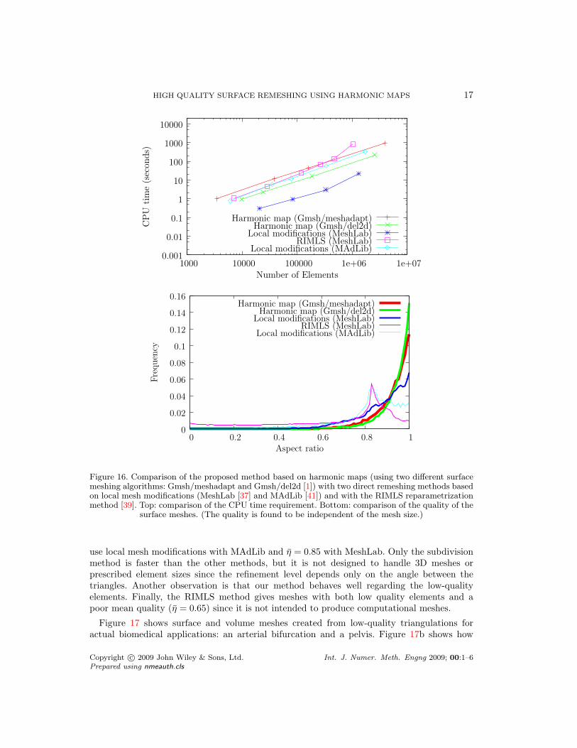
Figure 16. Comparison of the proposed method based on harmonic maps (using two different surfacemeshing algorithms: Gmsh/meshadapt and Gmsh/del2d [1]) with two direct remeshing methods basedon local mesh modifications (MeshLab [37] and MAdLib [41]) and with the RIMLS reparametrizationmethod [39]. Top: comparison of the CPU time requirement. Bottom: comparison of the quality of the

surface meshes. (The quality is found to be independent of the mesh size.)

use local mesh modifications with MAdLib and η = 0.85 with MeshLab. Only the subdivisionmethod is faster than the other methods, but it is not designed to handle 3D meshes orprescribed element sizes since the refinement level depends only on the angle between thetriangles. Another observation is that our method behaves well regarding the low-qualityelements. Finally, the RIMLS method gives meshes with both low quality elements and apoor mean quality (η = 0.65) since it is not intended to produce computational meshes.

Figure 17 shows surface and volume meshes created from low-quality triangulations foractual biomedical applications: an arterial bifurcation and a pelvis. Figure 17b shows how


18 J. F. REMACLE

the remeshed surface can be used to construct high-quality boundary layer meshes forcardiovascular blood flow simulations using MAdLib [41, 42].

(a) (b) (c)

Figure 17. Meshes created from STL triangulations obtained from CT-scans: a) Arterial bifurcationwith a uniform edge length on the boundary and a boundary layer mesh, b) zoom of the boundary

layer, c) Pelvis with a sinusoidal edge length.

5.2. Remeshing CAD patches

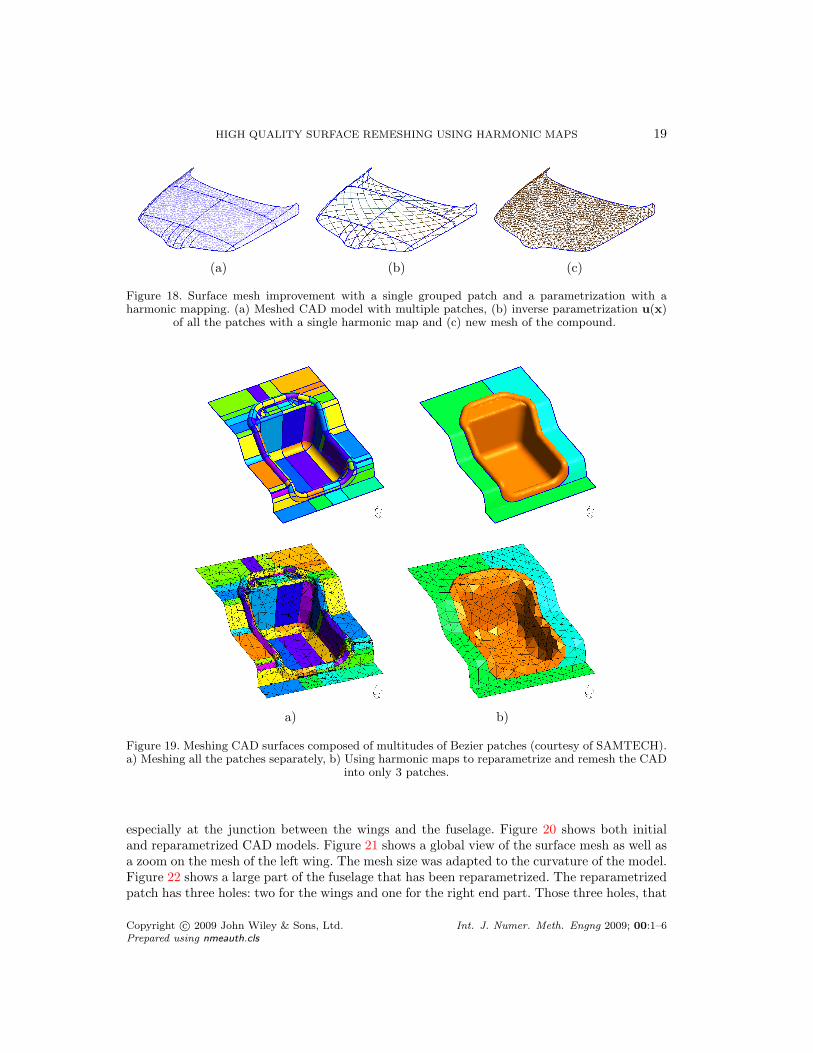
The next example shows a CAD model of a car hood made of 9 different patches that aresmoothly connected together (Figure 18). Standard surface meshers mesh each of those patchesseparately as shown in Fig. 18a. One common issue in engineering analysis is the presence ofsmall sub-patches for the description of one smooth surface which induces the presence of smallelements, leading to difficulties in the finite element analysis. It is therefore highly useful toreparametrize those patches into one single surface. This has been done in 2 steps: a meshhas been generated on the multiple patches (Fig. 18a) and the reparametrization (Fig. 18b)has been computed on this first mesh. Then we can remesh the whole compound using anyof the surface mesh generators available (Fig. 18c). Note that, in the case of multiple CADpatches reparametrization, points on the reparametrized surface are subsequently projectedon the exact CAD model. We use an initial triangulation that is conforming to the patchesso that every triangle of this initial triangulation lies on only one CAD patch. It is then easyto compute local CAD coordinates of every point in the new mesh and to compute thereaftertheir exact location on the CAD model.

The example of Figure 19 shows another CAD model composed of multiple patches thathas been reparametrized into three patches. This example shows clearly the advantage of theapproach when coarse meshes have to be generated. Here, reparametrizing a geometry allows togenerate smooth uniform meshes. Small details in the initial CAD model induce the generationof small ill-shaped elements. Note the number of reparametrized surfaces was done arbitrarily.

As another an example of a moderately complicated CAD model, we consider the AirbusA319. The aircraft is initially composed of 89 surface patches. After reparametrization, thisnumber has been reduced to 25 (Figure 20). Moreover, lots of curves were reparametrized,



(a) (b) (c)

Figure 18. Surface mesh improvement with a single grouped patch and a parametrization with aharmonic mapping. (a) Meshed CAD model with multiple patches, (b) inverse parametrization u(x)

of all the patches with a single harmonic map and (c) new mesh of the compound.

a) b)

Figure 19. Meshing CAD surfaces composed of multitudes of Bezier patches (courtesy of SAMTECH).a) Meshing all the patches separately, b) Using harmonic maps to reparametrize and remesh the CAD

into only 3 patches.

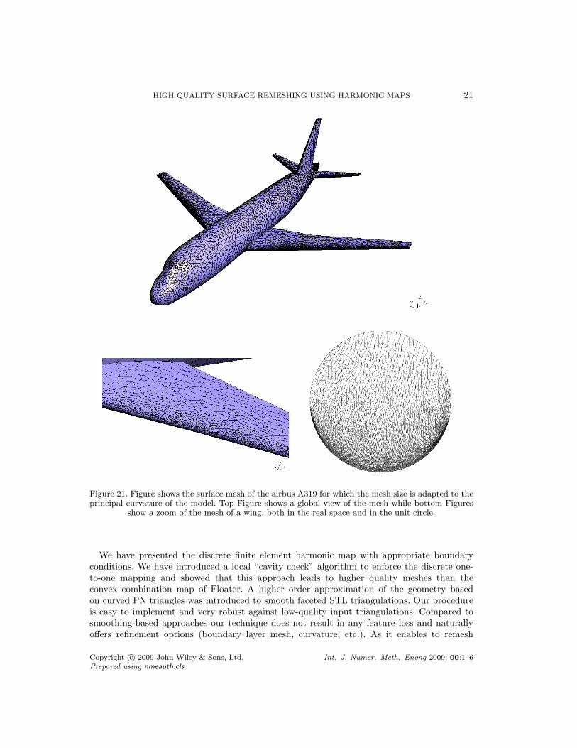
especially at the junction between the wings and the fuselage. Figure 20 shows both initialand reparametrized CAD models. Figure 21 shows a global view of the surface mesh as well asa zoom on the mesh of the left wing. The mesh size was adapted to the curvature of the model.Figure 22 shows a large part of the fuselage that has been reparametrized. The reparametrizedpatch has three holes: two for the wings and one for the right end part. Those three holes, that


20 J. F. REMACLE

are clearly visible in the parametric plane, are highly distorted. Even though, Gmsh’s surfacemeshers were able to produce high quality meshes (Figure 21) with such highly distordedinput.

(a) (b)

Figure 20. The model of the airbus A319. Figure(a) shows the initial CAD data made of 89 patchesand Figure(b) shows the reparametrized CAD made of only 25 patches.

5.3. Remeshing in Gmsh

As previously mentioned, the remeshing algorithm based on harmonic maps is implementedwithin the open-source software Gmsh. We show a simple example of how to use it. We supposethat we have an initial surface mesh and write the following text file ”remesh.geo”:

// Merge initial mesh (in .stl, .msh, .mesh, .brep, .medit, etc. format)Merge "bypass.stl";

// If the initial mesh contains different topological entities,// then re-create the topologyCreateTopology;

// If necessary, create a topological volumeSurface Loop(55) = {15, 16};Volume(56) = {55};

// Remesh the Edges and Faces (and Volumes) with harmonic mapsCompound Line(10) = {2, 3}; // merge 2 edgesCompound Surface(100) = {1:24}; // auto-detect boundaryCompound Volume(1000) = {56}

6. Conclusions and future work

In this paper, we have presented an efficient method for surface and subsequent volumeremeshing. The method is based on the parametrization of a genus zero surface with a harmonicmap.



Figure 21. Figure shows the surface mesh of the airbus A319 for which the mesh size is adapted to theprincipal curvature of the model. Top Figure shows a global view of the mesh while bottom Figures

show a zoom of the mesh of a wing, both in the real space and in the unit circle.

We have presented the discrete finite element harmonic map with appropriate boundaryconditions. We have introduced a local “cavity check” algorithm to enforce the discrete one-to-one mapping and showed that this approach leads to higher quality meshes than theconvex combination map of Floater. A higher order approximation of the geometry basedon curved PN triangles was introduced to smooth faceted STL triangulations. Our procedureis easy to implement and very robust against low-quality input triangulations. Compared tosmoothing-based approaches our technique does not result in any feature loss and naturallyoffers refinement options (boundary layer mesh, curvature, etc.). As it enables to remesh


22 J. F. REMACLE

Figure 22. Reparametrization of a large part of the fuselage. Left figure shows iso-contours of u andv. Center and right figures show the mesh in the parametric plane, i.e. inside the unit disk.

multiple CAD patches, the approach can be used to substantially reduce the time required toprepare CAD surface definition for surface mesh generation. The time required to generate thesurface mesh is less than 100s per 106 elements. Furthermore the generated elements have ahigh mean quality measure which is a clear demonstration of the suitability of the meshes forfinite element simulations.

We are currently working on an optimal numerical homology algorithm that willautomatically cut a initial surface onto different surfaces of genus zero with uniform geometricalaspect ratio. With this upcoming algorithm we hope to obtain a fully automatic method forhigh quality remeshing of any topological surface without any geometrical constraint.

Acknowledgements

J.-F. Remacle and C. Geuzaine would like to thank Dr. B. Levy for the fruitful discussionsthey had on reparametrization techniques at the Trophees du Libre 2009 in Soissons.

REFERENCES

1. Geuzaine C, Remacle JF. Gmsh: a three-dimensional finite element mesh generator with built-in pre- andpost-processing facilities. International Journal for Numerical Methods in Engineering 2009; 79(11):1309–1331.

2. Shewchuk JR. What is a good linear element? interpolation, conditioning, and quality measures. 11thInternational Meshing Roundtable, Laboratories SN (ed.), 2002; 115–126.

3. Szczerba D, McGregor R, Szekely G. High quality surface mesh generation for multi-physics bio-medicalsimulations. Computational Science – ICCS 2007, vol. 4487. Springer Berlin, 2007; 906–913.

4. Marcum DL, Gaither A. Unstructured surface grid generation using global mapping and physical spaceapproximation. Proceedings, 8th International Meshing Roundtable, 1999; 397–406.

5. Aftosmis M, Delanaye M, Haimes R. Automatic generation of cfd-ready surface triangulation from cadgeometry. AIAA Paper 1999; 1(09-0776).

6. Ito Y, Nakahashi K. Direct surface triangulation using stereolithography data. AIAA Journal 2002;40(3):490–496.

7. Bechet E, Cuilliere JC, Trochu F. Generation of a finite element mesh from stereolithography (stl) files.Computer-Aided Design 2002; 34(1):1–17.

8. Wang D, Hassan O, Morgan K, Weatheril N. Enhanced remeshing from stl files with applications to surfacegrid generation. Commun. Numer. Meth. Engng 2007; 23:227–239.



9. Borouchaki H, Laug P, George P. Parametric surface meshing using a combined advancing-front generalizeddelaunay approach. International Journal for Numerical Methods in Engineering 2000; 49:223–259.

10. Zheng Y, Weatherill N, Hassan O. Topology abstraction of surface models for three-dimensional gridgeneration. Engrg. Comput. 2001; 17(28-38).

11. Marcum DL. Efficient generation of high-quality unstructured surface and volume grids. Engrg. Comput.2001; 17:211–233.

12. Tristano J, Owen S, Canann S. Advancing front surface mesh generation in parametric space usingriemannian surface definition. Proceedings of 7th International Meshing Roundtable. Sandia NationalLaboratory, 1998; 429–455.

13. Laug P, Boruchaki H. Interpolating and meshing 3d surface grids. International Journal for NumericalMethods in Engineering 2003; 58:209–225.

14. M Attene MS B Falcidieno, Wyvill G. A mapping-independent primitive for the triangulation of parametricsurfaces. Graphical Models 2003; 65(260-273).

15. Bennis C, Vezien JM, Iglesias G. Piecewise surface flattening for non-distorted texture mapping. ACMSIGGRAPH Computer Graphics 1991; :237 – 246.

16. Maillot J, Yahia H, Verroust A. Interactive texture mapping. Proceedings of ACM SIGGRAPH’93, 1993;27–34.

17. Floater MS. Parametrization and smooth approximation of surface triangulations. Computer aidedgeometric design 1997; 14(231-250).

18. Greiner G, Hormann K. Interpolating and approximating scattered 3d data with hierarchical tensorproduct splines. Surface Fitting and Multiresolution Methods, 1996; 163–172.

19. Levy B, Petitjean S, Ray N, Maillot J. Least squares conformal maps for automatic texture atlas generation.Computer Graphics (Proceedings of SIGGRAPH 02), 2002; 362 – 371.

20. Sheffer A, Praun E, Rose K. Mesh parameterization methods and their applications. Found. Trends.Comput. Graph. Vis. 2006; 2(2):105–171.

21. Floater MS, Hormann K. Surface parameterization: a tutorial and survey. Advances in Multiresolution forGeometric Modelling 2005; .

22. Eck M, DeRose T, Duchamp T, Hoppe H, Lounsbery M, Stuetzle W. Multiresolution analysis of arbitrarymeshes. SIGGRAPH ’95: Proceedings of the 22nd annual conference on Computer graphics and interactivetechniques, 1995; 173–182.

23. Schoen R, Yau S. Lectures on Harmonic Maps. International Press, Harvard University, 1997.24. Alliez P, Meyer M, Desbrun M. Interactive geometry remeshing. Computer graphics (Proceedings of the

SIGGRAPH 02) 2002; :347–354.25. Floater MS. Parametric tilings and scattered data approximation. International Journal of Shape Modeling

1998; 4:165–182.26. Rado T. Aufgabe 41. Math-Verien 1926; :49.27. Choquet C. Sur un type de representation analytique generalisant la representation conforme et defininie

au moyen de fonctions harmoniques. Bull. Sci. Math 1945; 69(156-165).28. Floater MS. One-to-one piecewise linear mappings over trinagulations. Math. Comp 2003; 72(685-696).29. M P, G EM. Quasi-monotonic continuous darcy-flux approximations in 3-d for any element type. SPE

Reservoir Simulation Symposium, Houston TX, USA, 2007.30. Lee DT, Preparata F. An optimal algorithm for finding the kernel of a polygon. Journal of the ACM,

Volume 26 1979; 26(3):415–421.31. Icking C. earching for the kernel of a polygon: A competitive strategy using self-approaching curves. 11th

Annu. ACM Sympos. Comput. Geom, 1995; 258–266.32. Chang CT, Gorissen B, Melchior S. Fast computation of the minimal oriented bounding box on the rotation

group so(3). ACM Transactions on Graphics 2009, to appear; .33. Legrand S, E D, Hanert E, Legat V, Wolanski E. High-resolution, unstructured meshes for hydrodynamic

models of the great barrier reef, australia. Estuarine, coastal and shelf science 2006; 68(1-2):26–46.34. Shinagawa Y, Kunii T, Kergosien YL. Surface coding based on morse theory. IEEE Computer Graphics

and Applications 1991; 11(5):66–78.35. Boubekeur T, Alexa M. Phong tessellation. ACM Transactions on Graphics 2008; 27(5):141:1–141:5.36. Vlachos A, Peters J, Boyd C, Mitchell JL. Curved pn triangles. Proceedings on 2001 Symposium on

INteractive 3D graphics, 2001; 159–166.37. 3D-CoForm. Meshlab 2009. http://meshlab.sourceforge.net/.38. Loop C. Smooth subdivision surfaces based on triangles. Master’s Thesis, Department of Mathematics,

University of Utah August 1987.39. Oztireli A, Guennebaud G, Gross M. Feature preserving point set surfaces based on non-linear kernel

regression. EUROGRAPHICS 2009; 28(2).40. Compere G, Remacle JF, Marchandise E. Transient mesh adaptivity with large rigid-body displacements.

Proceedings of the 17th International Meshing Roundtable, vol. 3, Garimella R (ed.), Springer, 2008;


24 J. F. REMACLE

213–230.41. Compere G, Remacle JF. A mesh adaptation framework for large deformations. International Journal for

Numerical Methods in Engineering 2009; Accepted.42. Compere G, Remacle JF. Website of madlib: Mesh adaptation library 2008. http://www.madlib.be.


high quality surface remeshing using harmonic mapsgmsh.info/doc/preprints/gmsh_stl_preprint.pdf ·...

Documents