high resolution temperature monitoring in a …

Stud. Geophys. Geod., 52 (2008), 413−437 413 © 2008 Inst. Geophys. AS CR, Prague

HIGH RESOLUTION TEMPERATURE MONITORING IN A BOREHOLE, DETECTION OF THE DETERMINISTIC SIGNALS IN NOISY ENVIRONMENT

V. ČERMÁK, J. ŠAFANDA AND M. KREŠL

Institute of Geophysics, Acad. Sci. Czech Republic, Boční II/1401, 141 31 Praha 4, Czech Republic ([email protected])

Received: May 2, 2007; Revised: October 26, 2007; Accepted: November 15, 2007

ABSTRACT

Temperature was monitored as a function of time at several selected depth levels in a slim experimental borehole. The hole is 15 cm in diameter, 150 m deep, and effectively sealed from the influx of ground water by a plastic tube of 5 cm diameter. The mean temperature gradient is 19.2 mK/m. The borehole was drilled in 1993 and has been in equilibrium since then. The data obtained reveal that: (1) the temperature-time series showed a complex, apparently random oscillation pattern with amplitudes of up to 25 mK; (2) irregular temperature variations characterized by larger oscillations may alternate with relatively “quiet” intervals; and (3) the character of the oscillation may vary both in depth as well as in time and the transition between two distinct regimes may be sudden.

The Fourier analysis detected “red noise” behavior of the signal but did not highlight any specific peak(s) corresponding to periodicity in the measured temperature series. We employed a variety of techniques (roughness coefficient, local growth of the second moment, recurrence and cross recurrence plots) to reveal the deterministic framework of the system behavior. All above methods were proven to be quite robust in the face of noise, and enabled the discovery of structures hidden in the signals produced by complex natural processes.

Statistical analysis suggested the existence of a quasi-periodic intra-hole oscillatory convection. The temperature field in the hole has a dual-frequency structure, in which short period oscillations of about 10−30 minutes are superposed on longer variations of up to several hours. At certain conditions, so far not fully understood, the temperature oscillations may practically stop. The temperature remains within 1−2 mK for a period of several days when the oscillation pattern (convection ?) suddenly resumes.

Ke y wo rd s : borehole correction, recurrence analysis, temperature monitoring

1. INTRODUCTION

Temperature as a function of depth is generally measured by lowering a temperature probe to obtain either point-by-point temperature measurements or continuous T(z) record. Boreholes are usually filled with a fluid, and to acquire correct information, the measured

V. Čermák et al.

414 Stud. Geophys. Geod., 52 (2008)

(fluid) temperature is supposed to be equal to the (virgin) temperature of the surrounding rock strata. For further discussion let us presume that the borehole is in complete temperature equilibrium with no post-drilling disturbing effects and that there is no outward perturbation by groundwater movements. Those who measured temperature in boreholes in the pioneering days of early heat flow studies and used a thermistor probe connected to a Wheatstone bridge may remember that it was sometimes difficult to fully stabilize the measuring needle. The needle unrest manifested itself either by trembling, by short term variations or even by slow divergences that were indications of temperature instability.

A possible source of such thermal disturbances is fluid convection. Hales (1937) demonstrated that a fluid column in a vertical tube may become unstable when the temperature gradient exceeds a certain critical value. The problem was further discussed by Misener and Beck (1960), Garland and Lennox (1962) and Beck (1965) among others. Diment (1967) and Gretener (1967) experimentally proved the instability of the water column of a large diameter hole and reported that this instability manifested itself in vertical fluid movements with amplitudes of up to several diameters of the hole. The instability thus may produce temperature oscillations of several hundredths of a degree with periods ranging from minutes to hours, being proportional to the temperature gradient, borehole diameter and fluid properties.

2. BACKGROUND

Thermal convection of a fluid under different boundary conditions is an important physical problem in a variety of contexts. It has been most extensively studied, both theoretically as well as in laboratory, in the field of nonlinear dynamics. Temperature data obtained in boreholes may suitably serve as critical input to many fields of engineering, exploration, and research. In addition to large scale environmental signals borehole temperature logs may also contain small signals associated with factors such as heat transfer in compositionally and structurally heterogeneous subsurface and small scale convection in a water filled borehole.

The need of a thorough interpretation of the fine scale structure of the temperature signal has long been recognized (Haenel et al., 1988). The process of intra-hole convection, responsible for the fine scale temperature variations, can be discriminated as a generally deterministic process. This process operates on relatively short time scales with the characteristic times varying from a few seconds to days (e.g., Bodri and Čermák, 2005; and the references therein). In the presence of geothermal gradient, the relatively heavier cold fluid located above warmer and lighter fluid is forced to move downwards, the release of potential energy provides kinetic energy for the motion and the system becomes unstable. This instability is opposed by the frictional action of the fluid viscosity and thermal conductivity tends to equalize the temperature difference between the rising warmer and the sinking colder water masses. The motion thus occurs only when the destabilizing effect of the temperature difference is strong enough to overcome these obstacles.

The onset of motion can be indicated by the value of the dimensionless Rayleigh number:

High Resolution Temperature Monitoring in a Borehole

Stud. Geophys. Geod., 52 (2008) 415

( ) 3

2 1g T T dRa

k

αν−

= , (1)

where d is the characteristic length that generally is comparable with the diameter of the borehole; T2 − T1 is the temperature difference across the characteristic length; and g is the gravitational acceleration. Other quantities characterize fluid properties such as thermal diffusivity (k), thermal expansion coefficient (α), and kinematic viscosity (ν). The Rayleigh number depends on two specific parameters characteristic for a specific borehole, namely borehole diameter and geothermal gradient.

The mode of the intra-hole convection depends on another dimensionless parameter, the Prandtl number:

Pr kν= , (2)

which is a property of the particular fluid and not of the flow. As the Prandtl number decreases, relatively more rapid diffusion of heat compared with vorticity is observed. Most fluids have a Prandtl number greater than 1, but it may vary widely. Water that generally fills boreholes is typically at the low end of the range of the Prandtl numbers, Pr = 8 (ν = 1.15 × 10−6 m2/s, k = 0.143 × 10−6 m2/s). Finally, the depth of the borehole h is another relevant parameter even when it is much larger than d. This leads to non-dimensional parameters governing convection and providing dynamical similarity of the intra-hole convection in different systems, namely Ra, Pr and the so-called aspect ratio: A = h/d (h - depth of the borehole).

Instability occurs when the Rayleigh number exceeds its critical value; below this value, the fluid remains in equilibrium. For low Prandtl numbers, the critical Rayleigh number is above 2−5 × 103 at least for aspect ratios between 10 and 100 (Vest and Arpaci, 1969; Tritton, 1977; and the references therein). It should be mentioned, that the critical value of Ra for the onset of convection is system dependent and should be assessed for a given case. For example, one of the specific features of the intra-hole convection is that the viscous drag of the walls tends to restrain motions near the wall. It is reflected in the increase of the critical Rayleigh number for the onset of convection and in the simplification of its pattern.

In principle, temperature fluctuations caused by intra-hole convection can be measured by high resolution temperature monitoring within a borehole. Exact dynamics of the intra-hole fluid are determined by the stability properties of convection. Most probably, the intra-hole convection represents a system of more or less long cells, and the fluid motion represents the set of more or less similar orbits rather than single trajectory. In other words, fluid never returns exactly on the same trajectory. Except for the uncertainties produced by the instability of fluid convection and similarly to other data gained from natural systems, the signals measured in a borehole may contain a large amount of contaminating noise that in many cases completely masks the target deterministic signal structure. At least part of the observed noise can be attributed to heat conduction in a compositionally and structurally heterogeneous subsurface (Bodri and Čermák, 2005). Because the traditional linear methods of filtering (especially in very noisy situations) fail in unequivocal detection of the signal amongst the noise (Ghil and Yiou, 1996; Zbilut et al., 1998b), an extraction of the hidden signal buried in large amounts of noise can be

V. Čermák et al.


performed only by the use of complex computational techniques. An important advantage of temperature monitoring is that unlike most geophysical field situations that provide short data series, borehole monitoring may furnish long time data series that are suitable for nonlinear analysis methods.

3. DATA

The idea of conducting high resolution temperature monitoring in boreholes goes back to the experience earned during a field expedition to Kamchatka (Čermák et al., 2006). To check certain unexpected discrepancies observed in a number temperature logs, precise data loggers were located in two holes to run a long-term monitoring experiment. To verify the results, a similar experiment was later repeated in the Spořilov hole, that is located on the campus of the Geophysical Institute, Prague (50°02.43′N, 14°28.65′E, 270 m a.s.l.) and was drilled in the early nineties as the test site for long-term climate studies (Čermák et al., 2000). The 150 m deep and 10 cm diameter hole penetrated consolidated sediments, and the hole contains a plastic tube (5 cm in diameter) to prevent any disturbances due to ground water movement. The drilling history, the corresponding thermal equilibrium, and the conductivity structure of the surrounded rock strata are well documented (Šafanda, 1994; Štulc, 1995). Several monitoring experiments were performed in 2004−2005. All displayed intermittent, non-periodic oscillations of temperature of up to several hundredth of degree with sharp gradients and large fluctuations over all observed time intervals (Čermák et al., 2007a). These temperature variations were interpreted as an “oscillatory” convection occurring due to instability within the horizontal boundary layers between the individual convectional cells (Čermák et al., 2007b).

The present experiment focused on detailed synchronous temperature monitoring performed with five autonomous high resolution data loggers (all fixed to a single cable) and located at 85, 95, 100, 105 and 115 m depth (this depth includes the previously studied depth range). Each data logger is a cylindrical steel probe 160 mm long and 14 mm in diameter. As a matter of fact, no borehole is perfectly vertical and the loggers may be leaning against the casing. The presence of the loggers somehow narrows the internal space (in the present case by about 8%), and the surface quality of the borehole walls (casing) may affect the viscous drag. Here, we simplified the solution to an ideal case and did not considered such potential influence. The reorganization of the convection pattern (from single to double cells) was discussed e.g. by Koster and Müller (1984); for the simplification of the flow pattern in narrower slots see e.g. Lee and Korpela (1970) or Besinger and Ahlers (1982).

The sampling interval can be pre-selected from 1 sec to 15 minutes, we used 6 sec in the present experiment; the reported relative accuracy of the probe is 1 mK, and the memory capacity amounts up to 65000 data points. The whole experiment took 4.5 days (May 29 to June 2, 2004), and for further calculation, we have chosen two one-day-long (14401 data points) sections from the bulk of the monitoring results (sections A and B) (Fig. 1, Tables 1 and 2).



As seen, the temperature records do not show any obvious ordered pattern, and the dominant feature of all temperature time series are irregular changes of the character of temperature variations from noticeable larger oscillations to relatively “quiet” intervals of varying length. A transition in the mode of variations occurs below 105 m depth. While the amplitudes of the temperature oscillations in “normal” intervals vary between 10−40 mK, “quiet” intervals are characterized by order of magnitude lower amplitudes of 2−6 mK. In some cases (e.g. in the 105-minute time series), the system can “switch” its regime quickly after sudden temperature fluctuations that exceeded certain threshold in a form of a “burst”. Probably, such a “burst” causes a sudden increase of the Rayleigh number and initiates “switching” to another convection regime (Bodri and Čermák, 2005; Čermák et al., 2007a).

Fig. 1. Temperature time series (sampling interval 6 sec) measured at five depth levels (85 to 115 m) in borehole Spořilov. For practical reasons of interpretation two one-day-sections were selected (sections A and B) marked by grey shade. Lower panel shows the whole temperature records in the actual size, the upper panel shows three series to better illustrate various characters of the individual time series. Note e.g. the 105 m record when the record pattern abruptly changed and after approximately two days returned to the original appearance.

V. Čermák et al.


4. DATA ANALYSIS

4 . 1 . R o u g h n e s s C o e f f i c i e n t

The roughness coefficient is a single quantity that describes the frequency of the sharp temperature changes within the time series. For time series y1, y2, …, yN with a mean y ,

the roughness coefficient R can be calculated as:

( )

( )

21

2

2

2

N

i ii

N

ii

y y

R

y y

−=

=

−=

−

∑

∑ (3)

For a straight line R = 0, and for sine waves with periods of π, 2π and 4π it equals to 0.04, 0.01 and 0.0025, respectively. Roughness coefficients calculated for depth levels of sections A and B are presented in Table 3. While the roughness of the shallower

Table 1. Statistical characteristics and the slope value (b) of the power spectral density for 5 depth levels, Spořilov hole - section A.

Depth [m] Range of

Variations [K] Mean [°C] St. Dev. [K] Δf 1 b

85 0.011 11.323 0.0026 0−2.0 2.68 95 0.023 11.478 0.0050 0−2.0 2.95

100 0.032 11.565 0.0079 0−2.3 2.99 105 0.025 11.705 0.0043 0−2.5 2.75 115 0.003 11.891 0.0004 0−2.0 1.19

1 - range of the normalized frequency for which exponent b was estimated.

Table 2. Statistical characteristics and the slope value (b) of the power spectral density for 5 depth levels, Spořilov hole - section B.

Depth [m] Range of

Variations [K] Mean [°C] St. Dev. [K] Δf 1 b

85 0.025 11.340 0.0068 0−2.3 2.99 95 0.031 11.463 0.0071 0−2.3 2.83

100 0.040 11.537 0.0122 0−2.3 3.00 105 0.006 11.716 0.0018 0−2.5 1.95 115 0.002 11.891 0.0005 0−2.0 0.73

1 - range of the normalized frequency for which exponent b was estimated.



temperature time series is comparable with that of sinusoids that may hint of a hidden periodic framework in the measured signal, the roughness grows by more than an order of magnitude for both 115-m depth segments. Such growth is caused by the “spiked” appearance of temperature oscillations, when weak but often frequent temperature “jumps” occur one after the other, a characteristic feature for aperiodic and strongly irregular signals. Both coefficients, the range of temperature variations and the roughness, quantified the basic difference between “normal” and “quiet” sections as more noticeable/less frequent sudden changes and less noticeable/more frequent sudden oscillations of temperature, respectively. This contrast probably implies the fundamental difference of the signal creating processes. To corroborate this preliminary conclusion, we have employed more sophisticated statistical techniques describing the data in terms of the variance and autocorrelation on multiple temporal scales. Generally, such methods need certain data pre-processing (such as filtering and linear detrending) to assess weather the variable is normally or near-normally distributed.

Our calculations confirmed that the temperature-time data at all depth levels have normal Gaussian distribution. As an example, Fig. 2 shows the cumulative probability distribution (probability that a random fluctuation dT exceeds a fixed value T) for the 105-m interval of section A.

4 . 2 . C h a r a c t e r i z a t i o n o f S p e c t r a l H e t e r o g e n e i t y

Fourier transformation is a conventional method of analyzing time series data to determine the power (mean square amplitude) as a function of frequency and represents a useful tool to separate the variance of time series into a set of simple terms associated with different time scales (break up complex periodic function into individual peaks) as well as to test the detected peaks against the “red noise” background. We used the windowing Fourier transform method to estimate the heterogeneity of power spectra of the temperature signals. This method was applied to sections A and B of all 5 probes, and the calculations show that none of the temperature time series contains any significant linear trend so there is no need for data de-trending. Tapering” with 10% Hanning window was applied to both sides of the records before Fourier transformation. Two examples of spectra characteristic for the “normal” and “quiet” sections are presented in Fig. 3.

All calculated power spectra are qualitatively similar. Fourier analysis did not highlight any remarkable peak corresponding to a signal frequency and the background seems to be dominant. The spectra of all the time series are characterized by two

Table 3. Roughness coefficient for sections A and B of 5 depth levels, Spořilov hole.

Depth Level [m] Section A Section B

85 0.0299 0.0045 95 0.0084 0.0040

100 0.0033 0.0013 105 0.0116 0.0650 115 1.4532 1.8401

V. Čermák et al.


important features: continuity and so called “red noise” behavior (a slope towards longer time scales in the logarithmic representation of the power spectra). The “redness” can be attributed to the stochastic mechanisms where random high frequency fluctuations are integrated by the components of the system with slower response, while the low frequency fluctuations develop and grow in the amplitude with increasing time scale (Hasselmann, 1976). All the energy spectra obtained can be described by a single power law E(f) ~ f −b, where E(f) is the power spectral density and f is frequency. The exponent b can be interpreted as a measure of departure from the non-correlated random white noise. The scaling spectrum with b ≠ 0 has an “excess” of energy at low frequences that is known as a “red noise” (in the sense of Gilman et al., 1963).

The flattening of the power law spectrum (“white noise” with spectral exponent b = 0) is limited to high normalized frequency range between 2 and 3.7 (Fig. 3), which corresponds to short periods of 3 min to 12 sec. This flattening can be attributed to pure random noise in the measured data (e.g. the instrument’s inability to respond to frequent weak signals). The onset of the spectral plateau ultimately establishes the threshold of the frequency domain where useful signal can be measured with confidence. The flat sections of all calculated spectra are short embracing periods from few minutes to seconds (for sampling interval of 6 sec). In comparison with the one-day length of the investigated sections A and B, the white noise component is small, and in most measured frequency domains, the useful signal and “red noise” behavior dominates the noise level. Spectral exponents for all calculated spectra (Tables 1 and 2) are in range from 1 to 3.

For ordinary Brownian noise (b = 2) the change from one moment to the next is random and normally distributed. Threshold b = 2 divides two different types of stochastic

Fig. 2. The log-log plot of the cumulative probability distribution for the temperature record measured at the 105 m depth (section A). The Gaussian cumulative probability is shown for comparison.



behavior: either persistence (interval of 2 < b < 3) or antipersistence (interval 1 < b < 2). Persistent process implies positive correlation of subsequent temperature increments. In other words, if temperature fluctuation in one time interval is higher than average, it likely will be higher also in the next interval and vice versa. Such series exhibit weak random fluctuations superposed upon prolonged quasi-cycles that hints quasi-periodicity of temperature-forming process that can be associated with a small-scale steady state convection of fluid in the hole. This is the case found for depth levels of 85 to 100 m (both sections A and B) and also for the 105 m depth level (section A). Lower noise level (more obvious determinism) in the time series manifests itself as increasing spectral exponent. Extreme case of b = 3 means that the correlation coefficient between two successive increments is 1, and the function is differentiable (deterministic).

Spectral exponents calculated for “quiet” sections are not unanimous as for the “normal” ones and indicate two different patterns of temperature oscillations. For the 105 m depth level, section B exhibits a behavior close to the ordinary Brownian noise (random fluctuations), while both sections of the 115 m level showed a spectral exponent close to 1, suggesting (antipersistent) inversely correlated fluctuations. In this case the signal reveals a more “nervous”, rough appearance with frequent reversals. It does not exhibit any sign of periodicity and temperature never moves too far from the mean, resulting in the less pronounced oscillations. Such behavior is also indicated by a decreased range of temperature variations in comparison with the “normal” sections and an increased roughness coefficient. The close-to-one signal corresponds to the so called

Fig. 3. Power spectra and their power-law fits (straight line) for monitoring results for the 105 m depth record (sections A and B). The frequencies were normalized to the lowest frequency in the spectrum and the power spectral density was normalized to that at the lowest frequency. For the list of slope values (b) characteristic for the individual depth sections see Tables 1 and 2.

V. Čermák et al.


“flicker” of 1/f noise (Mandelbrot, 1999). This kind of noise appears in nature (usually described as “ubiquitous”), and in geology and geophysics, it was reviewed by Turcotte (1992).

4 . 3 . R e c u r r e n c e P l o t s

The differences between “normal” and “quiet” time series as well as quasi-periodicity supposed by two previous analyses can be visualized by means of the recurrence plots (RP). It is a two-dimensional image technique that presents hidden regularities invisible in the scalar time series in a manner that is instantly apparent to the eye, for example, whether it is periodic or random (Eckmann et al., 1987). In the experimental cases where unambiguous physical models are not available, the RP can provide useful information about observed processes that could not be easily obtained otherwise. Mathematically, this method expands a one-dimensional time series into a higher dimensional space. Essentially this technique is a form of autocorrelation. Among other merits, RPs are quite robust in the face of noise and are able to detect the deterministic component (the framework of the system behavior) even in noisy signals and can effectively characterize the geometry of their structure (Zbilut et al., 1998b).

As previously, we consider a temperature time series {yi} with N terms and form the

vector ( ),i d τY

( ) ( )( )1, , , ,i i i i dd y y yτ ττ + + −=Y … (4)

by using an embedding dimension d ≥ 2 and a time delay τ ≥ 1. The former quantity defines the number of the vector components, while the latter determines the time interval between neighboring components. The recurrence plot is formed by comparison of all

embedded vectors with each other. We use the Euclidean norm ,i j i jD = −Y Y as

a distance-measure between vectors. The calculated 2-D array of distances can be used as it is in the unthresholded recurrence plot (UTRP), when black represents small distances between the points, grey represents medium distances and white corresponds to large distances.

The thresholded recurrence plot (TRP) is defined as ( ), ,i j i jR Dε= Θ − , where ε is

a pre-defined fixed cut-off distance and Θ(x) is the Heaviside function. The values 1 and 0 given by this function can be visualized in a point map by black and white colors. Thus in

this case, the recurrence is defined as closeness of the state jX to the state iX . The use

of the cut-off distance (threshold) is caused by the fact that generally the system state is never repeated exactly, but only comes close to the initial state.

A single casual (i, j) point in the TRP diagram does not contain any information and only the whole array of points allows one to reconstruct the dynamic properties of the system. For illustration, see several simple cases of the TRP application in Fig. 4: (A) pure sine wave, where long straight parallel lines indicate periodic series, (B) square wave which exhibits a diagonal block-like structure, and (C) an opposite example of a random time series, namely Gaussian white noise with mean equal 0 and standard deviation



equal 1, which does not show any sign of regularity. It is of advantage that different values of cut-off distance do not influence the main features of the TRP and make them only thicker or thinner; smaller ε values leads to better distinction of small variations. In the present work, we have used both TRP and UTRP representations.

The RP technique has emphasized the fundamental difference between “normal” and “quiet” sections and has revealed that the structure of the persistent “normal” series is not as uniform as can be concluded from the results of the Fourier analysis. It clearly detected hidden periodicity that can be only hypothesized from the results of the previous analyses. The case is illustrated on temperature-time series from the 85 m depth (Figs. 5 and 6a,b). The TRP patterns contain numerous single points and brief periodic pieces (short diagonal strips). Such structure indicates the presence of certain unstable periodic orbits embedded in the chaotic attractor of a deterministic system. Although the existence of a diagonal structure is clear, no quantitative conclusion can be extracted. Similar structure was found, in chaotic windows of the logistic map by Zbilut et al. (1998a) and Marwan et al. (2002a). However, such texture is characteristic only for rare “flat” sections of the measured time series and hints of instability in the investigated intra-hole convection and the possibility of bifurcation. A more common kind of UTRP was characteristic of the bulk of the measured temperature time series, and contains many longer almost continuous diagonal bands characteristic of quasi-periodic dynamics (Fig. 6a). Due to influence of noise, the existing diagonal structure is often interrupted in comparison with an ideal case of a single sine wave presented in Fig. 4(left), but the existence of quasi-

Fig. 4. Illustration panel: recurrence plots TRP (d = 3, τ = 1, ε = 0.001) for several synthetic examples: (A) sine wave, (B) square wave, and (C) Gaussian white noise.

V. Čermák et al.


periodicity is clear. The distance between the diagonal lines is approximately 150−350 points which for the 6 sec reading interval correspond to periods of 15−35 min.

Certain potential oscillations with a considerably longer period existed, and an example is presented in Fig. 6b. The distance between the diagonal lines of approx. 4000 points corresponds to periods of 6−7 hours. These two distinct frequencies were found throughout the whole range of measurements up to 115 m depth.

Fig. 5. The TRP of the relatively very “flat” section of the temperature time series measured at 85 m depth (section A, 200th to 1200th data point; d = 10, τ = 10, ε = 0.001). Distance between individual points on the time axis equals to 6 sec. The curve in the upper panel represents the moving average window for 1000 consecutive data points (i.e., approximately 1.6 hour duration). The axes of the recurrence plot refer to data points.



Recurrence plots constructed for data measured at 115 m depth showed a specific texture that differs significantly from that existing at the upper depth levels (Fig. 7a). This texture contained a highly characteristic pattern that contains numerous vertical/horizontal lines and long patches of nearly constant values. The vertical/horizontal lines mark the segments of time series in which a state does not change or changes very slowly. Such block-like structure also hints of quasi-periodicity, however, of other kind than that produced by a sine wave. Blocks show that the state is “trapped” for some time (compare with the example illustrated for the TRP square wave, Fig. 4b). In natural dynamical systems, such pattern is a typical behavior of intermittency (Marwan et al., 2002b). The size of blocks gives an indication of the duration of such “trapped” states. For real periodic series, such as a square wave, these blocks will be equally sized, while for quasi-periodic time series they usually differ in size. For comparison, we present a recurrence plot (Fig. 7b) obtained for temperature monitoring at the bottom of the hole (Čermák et al., 2007a,b). The pattern is similar to those constructed for the 115 m depth level; however this likeliness is only illusory (see discussion below).

Fig. 6. a) Three UTRPs of different time intervals of the 85-m depth time series (sections A and B) showing typical diagonal structure (d = 10, τ = 10). b) The UTRP of the interval 7000−32000 of the 85-m depth time series showing diagonal structure corresponding to long period of temperature variations (d = 10, τ = 500, ε = 0.007). The axes refer to data points.

V. Čermák et al.


4 . 4 . L o c a l g r o w t h o f t h e s e c o n d m o m e n t ( L G S M )

The time dependent behavior of two or more physical processes can be recorded in a single time series. Spectral techniques yield an implicit “average” exponent b over a fixed scaling region. The contribution of different processes in the temperature signal can be assessed more precisely by the local growth of the second moment (correlation-like) technique that computes a separate value of b for each time increment used and, thus, represents a good test for multi-scaling. It computes the coefficient of correlation, r, between successive increments [ ]t t tI y yτ τ+ += − and [ ]2 2t t tI y yτ τ τ+ + += − , where t is

Fig. 7. a) The UTRPs of two intervals (3000−3800 and 4000−4800 data points) of the time series measured at 115 m depth (section A) (d = 10, τ = 10). b) The UTRP of the time series measured at the bottom of the Spořilov hole (d = 10, τ = 10) (Čermák et al., 2007a). The axes refer to data points.



time, τ is time lag, and y is temperature. Under the assumption that the increments have an expectation 0, the coefficient r can be calculated as:

( )

( ) ( )2

1 22 2

2

t t

t t

E I Ir

E I E I

τ τ

τ τ

+ +

+ +

=⎡ ⎤⎢ ⎥⎣ ⎦

, (5)

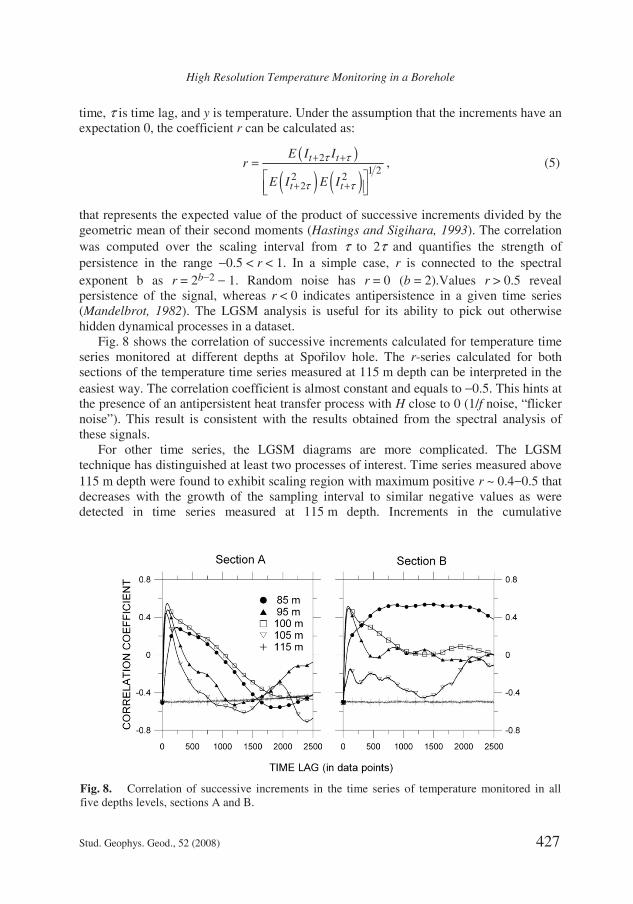
that represents the expected value of the product of successive increments divided by the geometric mean of their second moments (Hastings and Sigihara, 1993). The correlation was computed over the scaling interval from τ to 2τ and quantifies the strength of persistence in the range −0.5 < r < 1. In a simple case, r is connected to the spectral exponent b as r = 2b−2 − 1. Random noise has r = 0 (b = 2).Values r > 0.5 reveal persistence of the signal, whereas r < 0 indicates antipersistence in a given time series (Mandelbrot, 1982). The LGSM analysis is useful for its ability to pick out otherwise hidden dynamical processes in a dataset.

Fig. 8 shows the correlation of successive increments calculated for temperature time series monitored at different depths at Spořilov hole. The r-series calculated for both sections of the temperature time series measured at 115 m depth can be interpreted in the easiest way. The correlation coefficient is almost constant and equals to −0.5. This hints at the presence of an antipersistent heat transfer process with H close to 0 (1/f noise, “flicker noise”). This result is consistent with the results obtained from the spectral analysis of these signals.

For other time series, the LGSM diagrams are more complicated. The LGSM technique has distinguished at least two processes of interest. Time series measured above 115 m depth were found to exhibit scaling region with maximum positive r ~ 0.4−0.5 that decreases with the growth of the sampling interval to similar negative values as were detected in time series measured at 115 m depth. Increments in the cumulative

Fig. 8. Correlation of successive increments in the time series of temperature monitored in all five depths levels, sections A and B.

V. Čermák et al.


temperature deviation are positively correlated for short lags of approximately 100 to 250 points (10−25 min). Such characteristic times coincide well with the periods shown by the RPs. Further correlation falls to a near zero value at roughly 25−100 min, and for the most, time series continues to decrease with increasing time lag. The sections, where correlation coefficient is close to zero (random fluctuations), are short except of section B of the temperature time series measured at 95 and 100 m, where random noise represents significant part of the measured signal. For other time series, the values of correlation steeply turn into the negative part of the correlogram (antipersistent process, similar to that detected at 115 m depth). Thus, we have persistent system with the characteristic time of ~ 10−25 min, which can be probably associated with the quasi-periodic process detected in the RPs (small scale convection of fluid filling the borehole). This process dominates above the antipersistent behavior on shorter time scales. The antipersistent behavior is characteristic for the longer time scales. The structure of the signal observed in section A at 105 m depth is similar to that detected in shallower depths, while the structure of its section B represents the transition between shallower time series structure and the structure detected at 115 m depth. It is also contaminated by significant amount of random noise.

In addition to the CRP technique (next paragraph), the LGSM correlation provided the most perspective application for further studies. The simple selection of two (A and B) sections only provided comparisons between two possibly different time intervals. Fig. 9 offers a more detailed LGSM application, namely the r-coefficient distributions for 7 consecutive 10000 data-point long intervals covering all the 4.5 days experiment. While at the depth of 85 m all intervals generally suggest short-term persistence alternating with long-term antipersistence, at the 95 and 100 m depth levels the less noisy signal (compare the spectral exponents in Tables 1 and 2) is more homogenous and the “two-process” structure is distinct. In all these three depth levels, the temperature field became more “noisy” at the end of the whole observational interval. However, the conditions of occurrence and temporary intensification of random oscillations need a more systematic study. The data observed at the105 m depth levels are of prime interest, namely an apparent sudden change of the character of the T(t) record at the end of the second day of the experiment, equally as the sudden return to the previous conditions two days later.

4 . 5 . C r o s s - r e c u r r e n c e p l o t s

Cross recurrence plots are an extension of recurrence plots that were developed for the study of similarity/difference between two processes. We regard two time series {yi} and

{xi} with N terms that as previously form vectors ( ),i d τY and ( ),i d τX . As in the RPs,

we use the Euclidean norm ,i j i jD = −Y X as a distance-measure between vectors. The

thresholded cross-recurrence plot (TCRP) is defined as ( ), ,i j i jR Dε= Θ − . Now, a single

black point represents a similar state in system one {yi} and system two {xi}. As previously, a single point signifies nothing about common dynamics of both systems, and only the whole texture of the TCRP should be examined. All features characteristic for the TRP can be found also in the TCRPs (e.g., longer diagonal lines reveal epochs of a similar



dynamics of the two systems, periodicity). If the closeness of two systems is very high, similarly to the TRP, a main diagonal line will occur.

The power of the cross recurrence technique is demonstrated on a synthetic example in Fig. 10, which shows two delayed sine waves of the same period of 50 points, one of which is contaminated by Gaussian white noise (mean = 0, st. dev. = 1). Signal-to-noise-ratio (SNR) for such sine wave is 0.535. Both time series have a length of 500 data points. Their TCRP shows diagonal structure resulting from the similar phase space behavior of both functions. Diagonal structures are separated by gaps that occur because of the high fluctuations of the noisy sine wave. Due to the equal periodicity of both functions, the diagonals have a constant distance from each other that is equal to the period of compared waves. A time shift between two examined signals causes similar shift of the diagonal line observed on TCRP from the main diagonal (Marwan and Kurths, 2002).

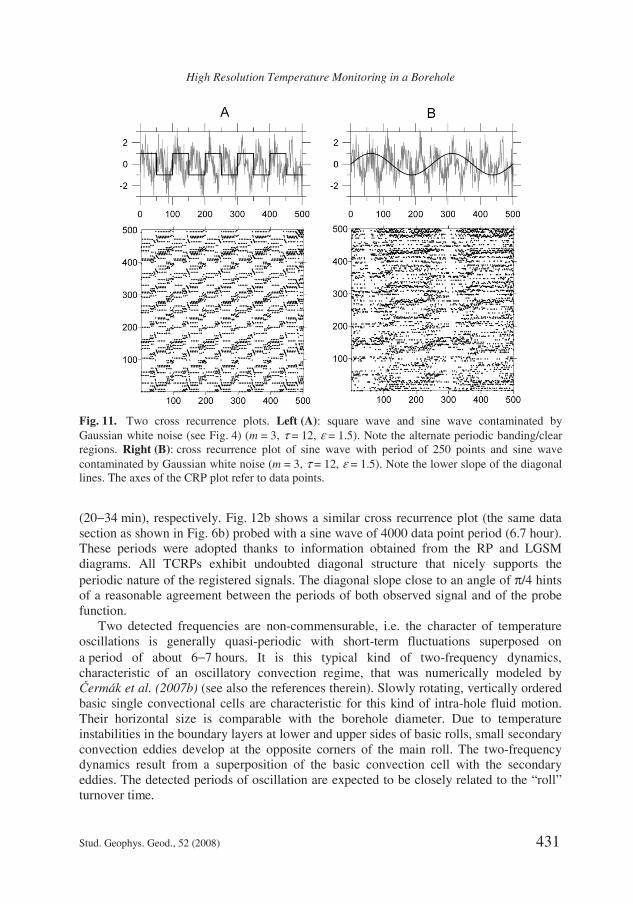
As shown by Zbilut et al. (1998a), the cross recurrence technique does not require extensive a priori models and can be used without exact knowledge of the target signal structure (typical situation in natural sciences). Two examples illustrate the property of the TCRPs. Fig. 11(left) shows the TCRP calculated for the sine wave contaminated by white noise probed with the square wave of the same period (Fig. 4). As previously, the clear

Fig. 9. Detailed analysis of the correlation of successive increments for time series calculated for seven 10000-data-point-intervals (each of approx.16.5 hour) covering all 4.5 days monitored time span. The last (7th) interval is shorter covering about 4000 data points only. Time lag is expressed in data points, for reading interval of 6 sec multiply by 6 to get time in sec.

V. Čermák et al.


diagonal structure hints of a similar periodic nature for the signals, and the distance between diagonal lines is equal to the period of variations. Fig. 11(right) illustrates a similar case, when sine wave+white noise signal was probed with a lower frequency sine wave (period of 250 points). The diagonal structure that hints the periodicity of the investigated signal is preserved, however, the slope of the diagonals changed. According to Marwan et al. (2002a) and Marwan and Kurths (2005), the slope of the line structures is determined by the time scaling of the corresponding trajectory segments and can be used for the adjustment of time scales of two compared data series. In other words, the slope of the diagonal lines can be used to rescale the time axes of two data series so that they can be synchronized. The authors also suggested the relationship between the time scales and the line structure in the CRP that can be used for the adjustment of the time scales in differently sampled time series and illustrated its applicability in geophysical measurements.

Fig. 12a shows three examples of the cross recurrence plots for the time series measured at the Spořilov hole (the same data sections as shown in Fig. 6a). Observed signals were probed with the sine waves of 260, 340 and 200 data point periods

Fig. 10. Cross recurrence plot (CRP) for two delayed sine waves (m = 3, τ = 12 and ε = 1.5). One of them was corrupted by additional white noise. The diagonal structure in the CRP occurs due to the similar phase space behavior of the functions. The axes of the CRP plot refer to data points.



(20−34 min), respectively. Fig. 12b shows a similar cross recurrence plot (the same data section as shown in Fig. 6b) probed with a sine wave of 4000 data point period (6.7 hour). These periods were adopted thanks to information obtained from the RP and LGSM diagrams. All TCRPs exhibit undoubted diagonal structure that nicely supports the periodic nature of the registered signals. The diagonal slope close to an angle of π/4 hints of a reasonable agreement between the periods of both observed signal and of the probe function.

Two detected frequencies are non-commensurable, i.e. the character of temperature oscillations is generally quasi-periodic with short-term fluctuations superposed on a period of about 6−7 hours. It is this typical kind of two-frequency dynamics, characteristic of an oscillatory convection regime, that was numerically modeled by Čermák et al. (2007b) (see also the references therein). Slowly rotating, vertically ordered basic single convectional cells are characteristic for this kind of intra-hole fluid motion. Their horizontal size is comparable with the borehole diameter. Due to temperature instabilities in the boundary layers at lower and upper sides of basic rolls, small secondary convection eddies develop at the opposite corners of the main roll. The two-frequency dynamics result from a superposition of the basic convection cell with the secondary eddies. The detected periods of oscillation are expected to be closely related to the “roll” turnover time.

Fig. 11. Two cross recurrence plots. Left (A): square wave and sine wave contaminated by Gaussian white noise (see Fig. 4) (m = 3, τ = 12, ε = 1.5). Note the alternate periodic banding/clear regions. Right (B): cross recurrence plot of sine wave with period of 250 points and sine wave contaminated by Gaussian white noise (m = 3, τ = 12, ε = 1.5). Note the lower slope of the diagonal lines. The axes of the CRP plot refer to data points.

V. Čermák et al.


Fig. 12. a) Cross recurrence plots of three different time series sections (85-m depth level shown in Fig. 8) probed with sine waves (see text). (d = 10, τ = 65, 85 and 50, resp., and ε = 2.235). Note typical diagonal structure. b) The CRP of the interval 7000−32000 section of the 85-m depth time series probed with a sine wave of 4000 measured points (6.7 hours) period (d = 10, τ = 1000, ε = 2.235). The axes of the CRP plot refer to data points.

b)

a)



When two frequencies become closer, they may disturb each other, and the oscillation system becomes non-periodic (Koster and Müller, 1984). Probably such state is detected in Fig. 5. Temporary transitions from quasi-periodic to non-periodic oscillations are generally observed at higher Rayleigh numbers and occur due to significant intermittency of oscillatory convection.

5. DISCUSSION AND CONCLUSIONS

Five-day long high-resolution temperature monitoring at the 85−115 m depth interval in the water-filled borehole Spořilov revealed small-scale temperature variations that can be attributed to the intra-hole fluid convection. Detected temperature oscillations are of two distinct types. The signal recorded above approx. 110 m depth (“normal” series) exhibits a noisy behavior with pronounced excursions from the mean value with the amplitudes of 10−40 mK. The “quiet” series, recorded below 110 m depth are characterized by “nervous” behavior with frequent temperature reversals, however, temperature does not change much and the oscillations are within the range of 2−6 mK only. In some cases (e.g. the 105-m time series), the system “switches” suddenly from one mode to another.

The use of formal statistical methods to interpret and describe the results of borehole monitoring together with its visualization can help to better understand the dynamics of this process. Together with traditional methods, such as Fourier analysis, the recently introduced powerful methods such as recurrence plots (RP) or local growth of the second movement (LGSM) can better detect very subtle patterns in time series that can be at best spotted on a classical visualization scheme (Fig. 13), but are difficult to describe in more detail. The use of modern techniques has quantified the differences between two revealed modes of temperature variations as well as provided deeper insight into the signal structure and the hidden regularities (deterministic framework of the signal).

We were primarily interested in the recognition of the potential periodic pattern that could be attributed to the borehole convection masked by noise. The Fourier analysis itself did not highlight any specific peak that might support the periodicity. However, already two-dimensional visualization of series by means of the RP has revealed a hidden two-frequency periodicity within the “normal” series. Although it is obvious that detected quasi-periodic process is complex due to the presence of noise, the existence of periodicity seems to be undoubted. For the detection of the characteristic times of temperature-forming processes the LGSM technique was applied. By combining the advantages of above methods we could proceed further and the application of the cross recurrence plot (CRP) the evidence of two-frequency convection with main period of about 6 to 7 hours and a secondary oscillation period between 20 and 34 minutes could be confirmed.

The character of the temperature field and its time pattern changes both in space (the monitoring results from the individual depth levels widely differ) and in time (the monitoring record at 105 m depth is a good example). The temperature signal recorded in the upper part of the investigated depth range hints rather at a noisy, positively correlated (persistent) state, while at greater depth, the signals can be characterized as negatively correlated (anti-persistent). The structure of the temperature signals recorded here is

V. Čermák et al.


complex and contains significant differences between its behavior in low and in high frequency domains. This fact reveals the existence of at least two distinct temperature forming processes, namely quasi-periodic persistent temperature variations in the lower frequencies (small-scale quasi steady-state fluid convection) and irregular anti-persistent high frequency oscillations. On the contrary at the base of the studied depth range (115 m), the local growth of the second moment technique revealed an almost constant correlation coefficient fluctuating around the value of −0.5 throughout all observational periods. This fact indicates only a single anti-persistent heat transfer regime.

The disappearance of the quasi-periodic signal at deeper levels may be a new phenomenon in borehole experimental studies. The mode of convective flow may vary from periodic, quasi-periodic to stochastic structures. As shown by experiments, fluids with low Prandtl number are quite susceptible to the instability. Generally, the change of dynamics is caused by the corresponding changes of the Rayleigh number along a borehole due to the local variations of the thermal gradient. At low Rayleigh numbers, convection may even cease. In our previous experiment (Čermák et al., 2007a,b)

Fig. 13. Map of temperature anomalies illustrating temperature vs. time changes within the depth interval 85 to 115 m depth during both one-day intervals studied (sections A and B). Temperature data were stripped for local temperature gradient of 0.0187 K/m. The temperature axes and scales are in mK.



temperature-time series monitored at the bottom of the Spořilov hole revealed only a single 1/f (“flicker-noise”) process similar to that now observed at 115 m depth. In the “bottom” case, the probe penetrated into soft rock debris, deposited at the bottom of the hole, which effectively prevented any contact between the probe and the surrounding borehole fluid and limited heat exchange to the conductivity only. The similarity of the spectral exponents and the LGSM results obtained for temperature time series monitored at bottom hole and at 115 m depth makes it enticing to assume that convection stopped there. However, two facts oppose such an idea:

1. The borehole logging showed that the local temperature gradient within the measured interval varies only by 1.5−2 times, thus noticeable variations of the Rayleigh number are hardly expected. Temperature in the “quiet” part of the 105-m-depth time series is slightly higher that in both neighboring quasi-periodic segments. Therefore the observed “quiet” regime scarcely can be attributed to a lower Rayleigh number. Because fluid viscosity tends to fall as temperature increases, slow natural growth of the Rayleigh number with depth can be expected. Within the 11−12°C interval, corresponding to an average range of temperature increase in the 85−115 m depth section in the Spořilov hole, the viscosity of water decreases by about 2.7%. It is doubtful that such fall can cause a noticeable change in the Rayleigh number.

2. As mentioned above, the 1/f noise appears very often in nature, and can be produced by a variety of physical processes.

A more probable explanation to the diverse character of the 115-m record may be related to a transition from a quasi-periodic convection to the chaotic state. As revealed by laboratory experiments as well as by numerical modeling (Ecke and Haucke, 1989), the injection of external noise to convecting fluid has a dramatic effect in some cases and can induce the reorganization of periodic motion into intermittent chaotic state. For time series

y1, y2, …, yN with the mean y the noise amplitude σ can be defined as the normalized

rms fluctuation in yi:

( )2iy y

yσ

−= ∑

. (8)

As seen from Table 4, the noise amplitude significantly grows at 100 m. This phenomenon is quite intriguing because it occurs directly above that level where a drastic

Table 4. Amplitude of noise σ.

Depth [m] Section A Section B

85 0.311 0.814 95 0.602 0.853

100 0.950 1.469 105 0.517 0.220 115 0.053 0.062

V. Čermák et al.


change of the temperature oscillation mode takes place. Thus, the possibility of noise induced intermittency cannot be rejected. On the other hand, the reasons for observed variations of noise amplitude are unknown and the results of Ecke and Haucke (1989) cannot be directly applied to the borehole convection, because their experiments were performed with lower Prandtl number fluids.

Acknowledgement: The technical problems of temperature monitoring were consulted with

several colleagues who all provided useful advice. The special thanks are due to Robert Kincler who assisted during the whole experiment by data collection. The manuscript was reviewed by Randy Keller and by anonymous reviewer. Both of them proposed numerous valuable comments which certainly improved the original version. The financial support provided by the Grant Agency of the Academy of Sciences of the Czech Republic under the project GAAV IAA300120603 and by the Grant Agency of the Czech Republic, project GACR 205/06/1181 was greatly appreciated.

References

Behzinger R.P. and Ahlers G., 1982. Heat transport and temporal evolution of fluid flow near the Rayleigh-Bénard instability in cylindrical containers. J. Fluid Mech., 125, 219−258.

Bodri L. and Čermák V., 2005. Miltifractal analysis of temperature time series: Data from boreholes in Kamchatka. Fractals, 13, 299−310.

Čermák V., Šafanda J., Krešl M. Dědeček P. and Bodri L., 2000. Recent climate warming: Surface air temperature series and geothermal evidence. Stud. Geophys. Geod., 44, 430−441.

Čermák V., Šafanda J., Bodri L., Yamano M. and Gordeev E., 2006. A comparative study of geothermal and meteorological records of climate change in Kamchatka. Stud. Geophys. Geod., 50, 674−695.

Čermák V., Šafanda J. and Bodri L., 2007a. Precise temperature monitoring in boreholes: evidence for oscillatory convection? Part I. Experiments and field data. Int. J. Earth Sci. (Geol. Rundsch.), doi: 10.1007/s00531-007-0237-4.

Čermák V., Bodri L. and Šafanda J., 2007b. Precise temperature monitoring in boreholes: evidence for oscillatory convection? Part II. Theory and interpretation. Int. J. Earth Sci. (Geol. Rundsch.), doi: 10.1007/s00531-007-0250-7.

Diment W.H., 1967. Thermal regime of a large diameter borehole: instability of the water column and comparison of air- and water-filled conditions. Geophysics, 32, 720−726.

Ecke R. and Haucke H., 1989. Noise-induced intermittency in the quasiperiodic regime of Rayleigh-Bénard convection. J. Stat. Phys., 54, 1153−1172.

Eckmann J.-P., Kamphorst S. and Ruelle D., 1987. Recurrence plots of dynamical systems. Europhys. Lett., 4, 973−977.

Garland G.D. and Lennox D.H., 1962. Heat flow in Western Canada. Geophys. J., 6, 245−262.

Ghil M. and Yiou P., 1996. Spectral methods: what they can and cannot do for climatic time series. In: Anderson D. and Willebrand J. (Eds.), Decadal Climate Variability: Dynamics and Predictability. Elsevier, Amsterdam, The Netherlands, 446−482.

Gilman D.L., Fuglister F.J. and Mitchell Jr., J.M., 1963. On the power spectrum of “Red Noise”. J. Atmos. Sci., 20, 182−184.



Gretener P.E., 1967. On the thermal instability of large diameter wells - an observational report. Geophysics, 32, 727−738.

Haenel R., Rybach L., and Stegena L., (Eds), 1988. Handbook of Terrestrial Heat-Flow Density Determinations. Kluwer Academic Publishers, London, U.K.

Hales A.L., 1937. Convection currents in Geysers. Mon. Not. Roy. Astr. Soc., Geophys. Suppl., 4, 122−131.

Hasselmann K., 1976. Stochastic climate models. Part I. Theory. Tellus, XXVIII, 473−485.

Hastings H.M. and Sugihara G., 1993. Fractals. A User’s Guide for the Natural Sciences. Oxford Univ. Press, Oxford, U.K.

Koster J.N. and Müller U., 1984. Oscillatory convection in vertical slots. J. Fluid. Mech., 139, 36−390.

Lee Y. and Korpela S.A., 1970. Multicellular natural convection in a vertical slots. J. Fluid. Mech., 42, 125−127.

Mandelbrot B.B., 1982. The Fractal Geometry of Nature. Freeman and Co, New York.

Mandelbrot B.B. 1999. Multifractals and 1/f Noise: Wild Self-Affinity in Physics (1963-1976). Springer-Verlag, New York.

Marwan N. and Kurths J., 2002. Nonlinear analysis of bivariate data with cross recurrence plots. Phys. Lett. A, 302, 299−307.

Marwan N. and Kurths J., 2005. Line structures in recurrence plots. Phys. Lett. A, 336, 349−357.

Marwan N., Thiel M. and Nowaczyk N.R., 2002a. Cross recurrence plot based synchronization of time series. Nonlinear Process. Geophys., 9, 325−331.

Marwan N., Wessel K., Meyerfeldt U., Schirdewan A. and Kurts J., 2002b. Recurrence-plot-based measures of complexity and their application to heart-rate-variability data. Phys. Rev. E, 66, 026702.

Misener A.D. and Beck A.E., 1960. The measurements of heat flow over land. In: Runkorn S.K. (Ed.), Methods and Techniques in Geophysics, Vol.1. Interscience Publishing, New York, 10−61.

Šafanda J., 1994. Effects of topography and climatic changes on the temperature in borehole GFU-1, Prague. Tectonophysics, 239, 187−197.

Štulc P., 1995. Return to thermal equilibrium of an intermittently drilled hole: theory and experiment. Tectonophysics, 241, 35−45.

Tritton D.J., 1977. Physical Fluid Dynamics. Van Nostrand Reinhold Company, New York.

Turcotte D.L., 1992. Fractals and Chaos in Geology and Geophysics. Cambridge Univ. Press, New York.

Vest C.M. and Arpaci V.S., 1969. Stability of natural convection in a vertical slot. J. Fluid Mech., 36, 1−15.

Zbilut J., Giuliani A. and Webber C., 1998a. Recurrence quantification analysis and principal components in the detection of short complex signals. Phys. Lett. A, 237, 131−135.

Zbilut J., Giuliani A. and Webber C., 1998b. Detecting deterministic signals in exceptionally noisy environments using cross-recurrence quantification. Phys. Lett. A, 246, 122−128.

high resolution temperature monitoring in a …

Documents