high strength steel fatigue
DESCRIPTION
Fatigue designTRANSCRIPT

Effect of TIG‐dressing on fatigue strength and weld toe geometry of butt welded connections in high strength steel Student: S.H.J. van Es [email protected] Student number: 1311255 March 2012 Graduation committee: Prof. ir. F.S.K. Bijlaard Structural Engineering, Delft University of Technology Dr. M.H. Kolstein Structural Engineering, Delft University of Technology Dr. ir. R.J.M. Pijpers Structural Engineering, Delft University of Technology Dr. ir. M.A.N. Hendriks Structural Mechanics, Delft University of Technology Ir. L.J.M. Houben Road and Railway Engineering, Delft University of Technology

2

3
Preface
During my bachelor thesis and my job as a student assistant I have experienced working in the Stevin II laboratory. When I needed to choose a subject for my master thesis, I quickly knew that I wanted experimental testing to be part of my project. After all, this may be the last chance to take part in experimental research with such depth and freedom of subject. My supervisor during my first two years as a student assistant was Richard Pijpers, who introduced me to his research of fatigue strength of welded connections in high strength steel. When there was an opportunity to perform a small experimental programme based on his larger database, this was a perfect chance for me to start my graduation thesis. An experimental programme cannot be performed alone, so I would like to thank the laboratory staff: Arjen van Rhijn
and John Hermsen who helped me preparating all specimens; Kees van Beek who programmed the software for the laser measurements and fatigue strength tests and finally Michele van Aggelen and Fred Schilperoort who have fixed many small problems I encountered in the laboratory. Of course I also thank my exam committee for the guidance during my thesis: Prof. ir. Frans Bijlaard, Dr. Henk Kolstein,
Dr. ir. Richard Pijpers and Dr. ir. Max Hendriks. The frequent meetings and the possibility to ask a quick question without appointment have been of great value. Finally I would like to thank my girlfriend Greta and my parents for the support during this project. Sjors van Es March 2012

4

5
List of symbols and abbreviations
Latin symbols a crack length parameter [mm] a* material constant in notch stress approach [mm] ai initial crack size [mm] af final crack size [mm] c crack width parameters [mm] C0 material constant in crack propagation calculation [Nmm‐3/2] d0,9 depth of V0,9 [mm] F applied force [kN] flm;Ni loading mode factor applicable to crack initiation life [‐] flm;Np loading mode factor applicable to crack propagation life [‐] flm;Nf loading mode factor applicable to total fatigue life [‐] fm mean stress and residual stress factor [‐] fmat material factor to determine fatigue limit of parent material [‐] fNi Ni/Nf [‐] fNp Np/Nf [‐] ft;Ni thickness factor applicable to crack initiation life [‐] ft;Np thickness factor applicable to crack propagation life [‐] ft;Nf thickness factor applicable to total fatigue life [‐] fuc influence factor for variation of undercut [‐] fwh influence factor for variation of weld height [‐] fθ influence factor for variation of weld toe angle [‐] FAT‐value see ΔσC h weld height [mm] ∆K range of stress intensity factor [Nmm
‐3/2] ∆Kth threshold value of ∆K below which no crack propagation occurs [Nmm‐3/2] Kf fatigue notch factor [‐] Kf;adj increased value of fatigue notch factor after adjustment of the
weld toe parameters in unfavourable direction [‐] Kt elastic stress concentration factor [‐] Kt;adj increased value of elastic stress concentration factor after adjustment of
weld toe parameters in unfavourable direction [‐] khs stress concentration factor at hot spot [‐] m slope of S‐N curve or material constant in crack propagation calculation [‐] N number of cycles [‐] NC number of cycles at FAT‐value [‐] ND number of cycles at constant amplitude fatigue limit [‐] Ni number of cycles to crack initiation [‐] Nknee number of cycles at fatigue limit [‐] NL number of cycles at cut‐off limit [‐] Np number of cycles during crack propagation [‐] Nf total number of cycles until failure [‐] Nup number of cycles at which the Basquin relation intersects with the yield line [‐] Ps probability of survival [‐] R stress ratio [‐] Reh specified minimum yield strength [N/mm2] R0,2 specified offset yield strength at 0,2% strain after unloading [N/mm2] Rm ultimate tensile strength [N/mm2] s multiaxiality coefficient to determine fictitious notch radius [‐] V0,9 highly stressed volume [mm3] w width of highly stressed volume [mm] Y compliance function in crack propagation calculation [‐] Greek symbols ε strain [‐] ρ notch radius [mm]

6
ρf fictitious notch radius [mm] ρ* material constant to determine fictitious notch radius [mm] θ weld toe angle; all angles are given in degrees [‐] Δσ stress range [N/mm2] ΔσC stress range at FAT‐value [N/mm2] ΔσD stress range at constant amplitude fatigue limit [N/mm2] ΔσL stress range at cut‐off limit [N/mm2] Δσmean mean stress range [N/mm2] Δσ95% stress range with 95% survival propability [N/mm2] σ0,2% offset yield stress at 0,2% strain after unloading [N/mm2] σa stress amplitude [N/mm2] σa;E endurable stress amplitude in plain material [N/mm2] σa;E;0 endurable stress amplitude in plain material at alternating load [N/mm2] σE;specimen endurable stress range in welded specimens [N/mm2] σE endurable stress range in plain material [N/mm2] σf stress below which infinite life is achieved [N/mm2] σhs stress at hot spot [N/mm2] σkaE endurable stress at the notch [N/mm2] σm mean stress [N/mm2] σnom nominal stress [N/mm2] σnotch stress at notch root [N/mm2] σr residual stress [N/mm2] σy yield stress [N/mm2] γ safety factor [‐] Abbreviations AW Indication that the value concerns as welded specimens BM Base material FZ Flusion zone or Fluid zone in case of TIG‐dressing HAZ Heat affected zone HSS High strength steel SG Strain gauge TIG Indication that the value concerns TIG‐dressed specimens (also: Tungsten Inert Gas) UC Undercut VHSS Very high strength steel WT Weld toe WM Weld material

7
Content
PREFACE............................................................................................................................................................. 3 LIST OF SYMBOLS AND ABBREVIATIONS...................................................................................................................... 5 CONTENT............................................................................................................................................................ 7
1 INTRODUCTION, PROBLEM ANALYSIS AND OBJECTIVES............................................................................................. 11
1.1 INTRODUCTION AND PROBLEM ANALYSIS ...................................................................................................... 11 1.2 OBJECTIVES ............................................................................................................................................ 11
2 INTRODUCTION IN HIGH STRENGTH STEEL, FATIGUE AND TIG DRESSING................................................................... 13
2.1 CHAPTER OUTLINE ................................................................................................................................... 13 2.2 INTRODUCTION IN HIGH STRENGTH STEEL ..................................................................................................... 13
2.2.1 Material.....................................................................................................................................................13 2.2.2 Possibilities and limitations .......................................................................................................................15
2.3 INTRODUCTION IN FATIGUE........................................................................................................................ 16 2.3.1 Definition ...................................................................................................................................................16 2.3.2 Parameters that influence the fatigue life.................................................................................................16 2.3.3 S‐N curve....................................................................................................................................................19 2.3.4 High strength steel and fatigue .................................................................................................................20
2.4 INTRODUCTION IN TIG‐DRESSING ............................................................................................................... 21 2.4.1 Weld improvement techniques..................................................................................................................21 2.4.2 TIG dressing process and influence on fatigue strength ............................................................................22
3 LITERATURE REVIEW: THEORY ................................................................................................................................... 23
3.1 INTRODUCTION AND CHAPTER OUTLINE........................................................................................................ 23 3.2 NOMINAL STRESS APPROACH ..................................................................................................................... 23
3.2.1 Principles ...................................................................................................................................................23 3.2.2 Calculation procedure................................................................................................................................23 3.2.3 Benefits, drawbacks and application.........................................................................................................24
3.3 STRUCTURAL STRESS APPROACH ................................................................................................................. 25 3.3.1 Principles ...................................................................................................................................................25 3.3.2 Calculation procedure................................................................................................................................25 3.3.3 Benefits, drawbacks and application.........................................................................................................26
3.4 CRACK PROPAGATION APPROACH................................................................................................................ 27 3.4.1 Principles ...................................................................................................................................................27 3.4.2 Calculation procedure................................................................................................................................29 3.4.3 Benefits, drawbacks and application.........................................................................................................29
3.5 NOTCH STRESS APPROACH......................................................................................................................... 29 3.5.1 Principles ...................................................................................................................................................29 3.5.2 Calculation procedure................................................................................................................................36 3.5.3 Benefits, drawbacks and application.........................................................................................................36
4 LITERATURE REVIEW: PRACTICE................................................................................................................................. 37
4.1 CHAPTER OUTLINE ................................................................................................................................... 37 4.2 LITERATURE REGARDING FATIGUE AND HIGH STRENGTH STEEL........................................................................... 37
4.2.1 Strength according to current design codes and recommendations .........................................................37 4.2.2 Behaviour of plain material .......................................................................................................................37 4.2.3 Behaviour of non‐plain material................................................................................................................38
4.3 LITERATURE REGARDING TIG‐DRESSING AND HIGH STRENGTH STEEL .................................................................. 41 4.3.1 TIG dressing process ..................................................................................................................................41 4.3.2 Strength improvement according to current design codes and recommendations ...................................41 4.3.3 Influences of TIG‐dressing on material and geometry ...............................................................................43 4.3.4 Influences of TIG dressing on fatigue strength ..........................................................................................46

8
5 TEST SETUP................................................................................................................................................................ 49
5.1 CHAPTER OUTLINE ...................................................................................................................................49 5.2 TESTING PROGRAMME..............................................................................................................................49
5.2.1 Identification of test specimens ................................................................................................................ 49 5.2.2 Preparation of specimens ......................................................................................................................... 49
5.3 TEST SETUP.............................................................................................................................................50 5.3.1 Measurement of weld geometry............................................................................................................... 50 5.3.2 Measurement of fatigue life ..................................................................................................................... 51 5.3.3 Measurement of material hardness.......................................................................................................... 52
6 PROCESSING AND RESULTS OF LASER MEASUREMENTS ............................................................................................ 53
6.1 CHAPTER OUTLINE ...................................................................................................................................53 6.2 TEST OUTPUT AND PROCESSING LASER MEASUREMENTS...................................................................................53
6.2.1 Test output................................................................................................................................................ 53 6.2.2 Determining the weld radius..................................................................................................................... 55 6.2.3 Determining the weld toe angle, weld height and undercut..................................................................... 59
6.3 RESULTS ................................................................................................................................................59 6.3.1 Observed geometries ................................................................................................................................ 59 6.3.2 Comparison between rolled and cast steel ............................................................................................... 60 6.3.3 Comparison between different steel grades ............................................................................................. 67 6.3.4 Distribution of weld geometry parameters ............................................................................................... 67 6.3.5 Evaluation of influence of TIG‐dressing..................................................................................................... 72
7 PROCESSING AND RESULTS OF FATIGUE TESTS AND HARDNESS MEASUREMENTS..................................................... 73
7.1 CHAPTER OUTLINE ...................................................................................................................................73 7.2 TEST OUTPUT AND PROCESSING ..................................................................................................................73
7.2.1 Test output................................................................................................................................................ 73 7.2.2 Determining Ni, nominal stress and stress ratio........................................................................................ 74
7.3 RESULTS OF FATIGUE TESTS ........................................................................................................................74 7.4 RESULTS OF HARDNESS MEASUREMENTS.......................................................................................................76 7.5 RESULTS OF CRACK MONITORING ................................................................................................................76
8 ANALYTICAL DETERMINATION OF FATIGUE STRENGTH.............................................................................................. 77
8.1 INTRODUCTION AND CHAPTER OUTLINE ........................................................................................................77 8.2 FACTORS DETERMINING FATIGUE STRENGTH..................................................................................................77 8.3 DETERMINATION OF STRESS CONCENTRATION FACTOR AND FATIGUE NOTCH FACTOR ............................................77
8.3.1 FEM analysis of weld toe........................................................................................................................... 78 8.3.2 Determination of Kt................................................................................................................................... 84 8.3.3 Determination of Kf ................................................................................................................................... 88
8.4 DETERMINATION OF MEAN STRESS FACTOR ...................................................................................................91 8.5 DETERMINATION OF THICKNESS FACTOR .......................................................................................................92 8.6 DETERMINATION OF LOADING MODE FACTOR ................................................................................................92 8.7 PREDICTION OF FATIGUE STRENGTH CURVE ...................................................................................................92
9 ANALYSIS OF FATIGUE TEST RESULTS......................................................................................................................... 93
9.1 CHAPTER OUTLINE ...................................................................................................................................93 9.2 ANALYSIS OF RAW DATA............................................................................................................................93
9.2.1 Exclusion of data....................................................................................................................................... 93 9.2.2 Adjustment of test data ............................................................................................................................ 95 9.2.3 Statistical analysis..................................................................................................................................... 97
9.3 FITTED S‐N CURVES .................................................................................................................................99 9.3.1 Raw data................................................................................................................................................... 99 9.3.2 Adjusted data.......................................................................................................................................... 100 9.3.3 Discussion ............................................................................................................................................... 102
9.4 COMPARISON .......................................................................................................................................102 9.4.1 Comparison of data with design codes ................................................................................................... 102 9.4.2 Comparison of data with as welded fatigue tests................................................................................... 106 9.4.3 Comparison of data with analytical determination of fatigue strength.................................................. 115
9.5 EVALUATION OF TIG‐DRESSING INFLUENCE.................................................................................................124

9
10 CONCLUSIONS AND RECOMMENDATIONS............................................................................................................. 125
10.1 CONCLUSIONS.................................................................................................................................. 125 10.1.1 Influence of TIG‐dressing of fatigue strength of butt welded specimens.................................................125 10.1.2 Influence of TIG‐dressing on weld geometry of butt welded specimens..................................................125 10.1.3 Theoretical influence of changed weld geometry on behaviour of TIG‐dressed specimens.....................126
10.2 EVALUATION AND RECOMMENDATIONS................................................................................................. 126 10.2.1 Assumptions and approximations ...........................................................................................................126 10.2.2 Recommendations for further research...................................................................................................126
ANNEX A : REFERENCES .............................................................................................................................................. 129
ANNEX B : TEST SPECIMENS........................................................................................................................................ 131
ANNEX C : FATIGUE TEST DATA................................................................................................................................... 133
ANNEX D : MATERIAL CERTIFICATES ........................................................................................................................... 135
ANNEX E : PRODUCTION DATA SHEETS TIG DRESSING ................................................................................................ 167
ANNEX F : MATLAB SCRIPTS TO PROCESS WELD GEOMETRY DATA ............................................................................. 177
ANNEX G : COLLABORATION WITH TNO: ACOUSTIC EMISSION ................................................................................... 183
ANNEX H : HARDNESS MEASUREMENTS..................................................................................................................... 185
ANNEX I : CRACK MONITORING RESULTS.................................................................................................................... 205
ANNEX J : DIANA MODEL............................................................................................................................................ 211

10
11
1 Introduction, problem analysis and objectives
1.1 Introduction and problem analysis In most design codes and in common engineering practice, the fatigue strength of welded high strength steel structures is
assumed to be comparable with the fatigue strength of mild steel structures. It is shown in literature (Maddox, 1991; Gurney, 1979) that perfect smooth specimens of high strength steel perform
better in fatigue tests than their mild steel counterparts. However, as soon as discontinuities, notches, surface roughness and all other imperfections that are unavoidable in practice are taken into account, the advantage of high strength steel quickly diminishes. To recover some of the advantages of high strength steel, several options can be used. The combination of welds and
other geometrical stress raisers can be omitted by design (for example by using cast steel nodes in trusses). Another possibility, which can also be combined with the aforementioned solution, is a weld improvement. Weld improvements are procedures executed after welding to improve the fatigue behaviour of the weld area by reducing tensile residual stresses, improving geometry, removing weld flaws and inclusions or a combination of these improvements. This research will focus on a weld improvement method called TIG dressing, in which the weld toe is remelted to provide a smoother weld profile. The procedure of TIG dressing has proven on fillet welds to be beneficial for both low strength and high strength steels in earlier research, but this effect is not always taken into account in current design codes and recommendations. This research will compare TIG‐dressed specimens with similar as welded specimens from the same material batches and
will attempt to explain differences in fatigue strength, based mainly on geometry changes.
1.2 Objectives The objectives of this study are:
Determine the fatigue strength of TIG dressing on various high strength steel butt welded specimens in relation to the fatigue strength of similar, as welded specimens
Describe the change of weld toe geometry due to the TIG dressing process on different high strength steel butt welded specimens
Relate the alleged improved fatigue strength by TIG dressing to the changed geometry by means of a theoretical analysis
To accomplish these objectives, a method needs to be found to accurately measure and describe the weld profile in a consistent way. Furthermore fatigue tests will be executed on material from the same production batches as used in an earlier research by Pijpers (2011). From this research, fatigue data and adjustment factors for various geometrical and loading parameters will be used. To gain insight into the current state of knowledge and a theoretical background to couple the weld geometry to fatigue strength, this study will start with a literature research into fatigue, high strength steel and TIG‐dressing.

12

13
2 Introduction in high strength steel, fatigue and TIG dressing
2.1 Chapter outline This chapter gives a general introduction in high strength steel, its production processes, possibilities and limitations.
Then a general introduction in fatigue is given, where the influencing factors of the fatigue process are discussed. The material and the process of fatigue are then combined. Finally a short explanation of the TIG‐dressing process is given and its effects on the material and fatigue behaviour.
2.2 Introduction in high strength steel
2.2.1 Material High strength steels are steels with a higher yield and tensile strength than the most commonly used steels. In current
practice in Europe, the steel grades S235 and S355 are most commonly used for mild steel structures. These steel grades have a yield strength of at least 235 and 355 N/mm
2, respectively. High strength steels have a specified minimum yield strength (Reh) higher than 355 N/mm2. Common high strength steels (HSS) range from S355 to S690. Higher strength steels are referred to as very high strength steels (VHSS). Again the steel grade refers to a specified minimum strength, but because higher strength steels do not always show a clear yield point, the specified ‘yield’ strength is the stress at which after unloading a permanent deformation of 0.2% remains (R0.2) (see figure 2.1).
figure 2.1 Stress strain relationship for a high strength steel; A is the proportionality limit, B the elastic limit, y the yield point. Line C is used to determine the point where a permanent deformation of 0.2% remains: the specified
‘yield’ point. (source: Engineering Archives, 2008)
High strength steels can be manufactured in different ways. The most common high strength steels are normalized steel, thermomechanically rolled steel and quenched and tempered steel. All these manufacturing processes are focussed on grain size reduction, which has a beneficial influence on the strength. Normalized steel and thermomechanically rolled steel are available in moderate high strengths (up to S460). Quenched and tempered steel is available in higher strengths (VM publication 125, 2008). The different treatments have their influence on the microstructure of the material. The microstructure of steel depends,
among other things, on the carbon content, temperature and cooling rate. In figure 2.2 the iron‐carbon diagram is shown. The three important phases are liquid (L), ferrite (α) and austenite (γ). Other forms are cementite (Fe3C) and pearlite (α+Fe3C). Austenite is formed above the transition temperature (for most carbon contents 723° C) and will transfer back to ferrite when cooled down. The possible excess of carbon, which is almost always the case when carbon is present, causes cementite to be formed. However, when the steel is cooled down fast, the austenite will change to ferrite oversaturated with carbon. This structure, called martensite, has a hard, crystalline and brittle structure with limited ductility. For this reason, steel consisting of martensite should be checked for sufficient ductility. As martensite is not an equilibrium phase, it is not visible in the iron‐carbon diagram. Another possible crystalline structure is bainite. Bainite is created when austenite

14
is cooled quickly, but not so quickly that martensite forms. Bainite consists of ferrite with a lot of dislocations combined with cementite. The dislocations make the ferrite harder than ordinary ferrite.
figure 2.2 The iron‐carbon diagram (source: KEYtoMETALS.com)
Normalized steel mainly gains its strength by alloyed elements. The toughness of the steel is kept within boundaries by the normalizing treatment, but the treatment also raises the strength to a certain extent, especially the ultimate tensile strength. To normalize the steel it is heated to about 920° and then cooled by air. Thermomechanically rolled steel has a low content of alloying elements and mainly gains its strength by grain size
reduction. This is achieved by controlling and limiting the temperature during the end stages of the rolling. The relatively low temperature during the final deformation of the components requires rather strong rolling equipment. When the material is processed further, heating beyond the transition temperature is not allowed to prevent loss of strength. Quenched and tempered steel is quickly cooled down to achieve high strength. This produces a very strong, very hard
and very brittle material. To reduce hardness and restore ductility the material is reheated to a temperature below the transition temperature. The energy for reheating can also be supplied by the core of thicker materials when only the perimeters are quenched. This is called quenched self‐tempered steel. The three production methods each leave a characteristic microstructure. Normalized steel consist of fine grained ferrite
and pearlite. Thermomechanically rolled steel starts with long austenite grains caused by the rolling processes. When cooled down a very fine grained ferrite structure is created. The microstructure of quenched and tempered steels mainly shows bainite and martensite in a crystalline structure. The different microstructures are depicted in figure 2.3.

15
figure 2.3 From left to right; microstructures of normalized S460, thermomechanically rolled S460 and quenched and tempered S1100 (source: VM publication 125, 2008)
2.2.2 Possibilities and limitations
Possibilities
High strength steel offers designers certain advantages, but it also has some drawbacks. The first advantage of high strength steel is directly related to its high strength: less material is needed to resist a certain force. Structures made of high strength steel can therefore be made lighter than their conventional counterparts. This is especially beneficial in movable structures, for example a movable bridge or mobile crane. Also most offshore structures benefit from this, because the transport to the building site on barges is an important part of the design. The second advantage is related to welded connections. In general, high strength steel structures have smaller plate thicknesses. Because the volume of added weld material increases quadratic with increasing thickness of the plates to be connected, a significant cost reduction could be made here, especially in western countries where wages are high.
figure 2.4 Schematic view of the economic advantages of high strength steel (source: VM publication 125, 2008)
Limitations
A large disadvantage of high strength steel is the material cost and availability. Conventional mild steels are more readily available and more easily produced and are therefore cheaper. High strength steels that are available, are mostly only available as plate material and not as profiles. This disadvantage may be outweighed by the reduction of welding costs and transportation costs. Another aspect of high strength steel is the fact that the Young’s modulus does not increase with increasing strength. For simple beam structures, high strength steel will therefore more easily reach the deformation limits set by the design code or dictated by secondary structures, such as internal walls and windows, than conventional steel structures. Structures that are stiff by their nature, such as truss structures, can overcome this problem. For the same reason, stability of high strength steel structures and components always needs attention. For columns, high strength steel therefore is only beneficial with highly loaded columns with relatively short buckling lengths, for example in high rise buildings. In beam structures, a high strength steel girder will probably not be a class 4 cross section. In tensile elements stability problems obviously cannot occur and therefore they can be very slender, with the exception of the area in which connections are made. A bolted connection can cause problems, because the yield strength (or 0.2% proof stress) is much closer to the tensile
strength then it is for ordinary steels. The reduction of this ratio with increasing strength is visible in figure 2.5. The allowable cross section reduction by holes is therefore limited. In general, all high strength steel structures and details should be checked for sufficient deformation capacity because of the lower ultimate strain of higher strength steels (see figure 2.5). Welded connections are possible in high strength steel, but current welding materials are limited to an ultimate strength of 900 N/mm2. For steel grades higher then S890 this will have consequences for the welded connections. Finally, the fatigue behaviour of high strength steel structures is commonly regarded as the same as for standard steel
structures. While a plain, polished specimen does show increasing fatigue strength with increasing yield strength, the addition of surface roughness, imperfections, notches and residuals stresses, all caused by production or welding, severely

16
reduce the fatigue strength of real structures and limits it to a level comparable with the fatigue strength of mild steels. This will be elaborated on in paragraph 2.3.4.
figure 2.5 Overview of material behaviour of steel with increasing strength (source: VM publication 125, 2008)
2.3 Introduction in fatigue
2.3.1 Definition Fatigue can be defined as the mechanism whereby cracks grow in a structure (ESDEP). These cracks grow under
fluctuating stresses, generated by fluctuating loads. Failure of a fatigue loaded structure occurs when the crack has reduced the cross section by such an amount, that the remaining cross section cannot carry the applied tensile loads. Fatigue can occur after a relatively low amount of cycles to very large numbers of cycles. In general, fatigue can be
divided into low cycle fatigue, medium cycle fatigue and high cycle fatigue. Exact boundaries between these three regimes are not apparent. Eurocode limits its use for applications with more than 104 cycles, which could be seen as a suitable boundary between low cycle and medium cycle fatigue.
2.3.2 Parameters that influence the fatigue life In fatigue, a number of parameters are important, primarily regarding the stresses in the material (see figure 2.6): N = the number of cycles ∆σ = the stress range. The stress range is defined as the maximum stress minus the minimum stress σm = the mean stress σa = the stress amplitude (half of the stress range)
R = the stress ratio: min
max
R

17
figure 2.6 Description of a fluctuating stress (source: ESDEP)
The mean stress influences the fatigue strength of the material. When the mean tensile stress increases, the fatigue capacity decreases. This has been derived by different authors, all showing roughly the same behaviour, see figure 2.7. When the static strength of steel increases, a higher mean stress in fatigue conditions can be endured. However, the sensitivity to the mean stress increases with increasing static strength (Haibach, 2006), resulting in a steeper line in figure 2.7.
figure 2.7 Mean stress effect shown in a Haigh diagram (source: ESDEP)
In principle, compressive stresses prevent cracks from opening, and therefore growing. Therefore, compressive stresses in theory increase the fatigue life of components. However, in most structures residual tensile stresses are present as a result of production and welding. This means that cracks in areas of the structure that are nominally under constant compression can still show crack growth. Therefore the mean stress effect is not always present in actual structures. For welded structures the residual stresses can be in the order of the yield limit, which severely reduces the fatigue strength. This is closely related to the mean stress effect, because a crack cannot distinguish a residual stress from a mean stress, and is called residual stress effect. Besides the stress also the geometry of the material has a large influence on the fatigue strength. Fatigue cracks start at
small defects in the material. These defects, called notches, can occur at the surface of the material due to roughness, inclusions or surface defects, at large discontinuities such as bolt holes or at small discontinuities, for example near the weld. At these notches the stress is concentrated, thereby increasing the chance of a fatigue crack occurring in that area. This is known as the notch effect.
figure 2.8 Examples of discontinuities where cracks can occur; on the left a large discontinuity: a cope hole' on the right, on smaller scale, a small discontinuity: a weld (source: ESDEP)
Corrosion at these discontinuities can further decrease the fatigue strength. Also in plain specimens there is a clear influence of corrosion on the fatigue strength, see figure 2.9.

18
figure 2.9 Influence of corrosive environments on the fatigue strength of materials (source: ESDEP)
The size of the specimen also influences the fatigue strength. When the size of a specimen increases, the fatigue strength drops. The total strength of the component may increase, but the allowable stress decreases. This is known as the size effect, and is caused by (ESDEP):
A statistical effect. When the size of a component increases, the chance of a ‘weak link’, in the form of a notch, small inclusion or residual stress, increases. Therefore also the chance of an initiating crack increases.
A technological size effect. The production processes and their associated surface conditions upon delivery have an influence on the fatigue strength of a component.
A geometrical size effect. When the thickness of a plate increases the stress gradient at a notch (in figure 2.10 a weld) decreases. When the inclusions or surface defects have the same size as they have in a thinner plate, the stresses at the tip of the defect are higher in the case of a thick plate (see figure 2.10).
A stress increase effect. When the plate thickness increases, the notch size in general does not scale up to the same amount, or may not scale up at all.

19
figure 2.10 Influence of the plate thickness on the fatigue strength (source: ESDEP)
Finally there is the effect of the material strength. When the material size increases the fatigue strength of the plain material also increases. However, when a crack occurs, the crack growth rate in all steels is roughly the same. This means that once a crack is initiated, all steels have a similar lifetime until failure when exposed to the same stress. Therefore high strength steels can only show a longer fatigue life if the material can longer resist crack initiation, this will be further elaborated on in 3.4. Because in actual structures plain steel always needs a connection, there will always be notches, stress raisers and, in the case of welding, inclusions present, which severely reduce the crack initiation life. Therefore, in current design codes, high strength steel structures mostly are regarded to have a fatigue strength comparable with standard steel structures. This subject is studied further in 2.3.4 and 4.2.
figure 2.11 Material strength effect. Plain machined specimens show a clear increase in fatigue strength when the material strength increases. At the same time it is clear that this increase is not entirely visible for notched specimens
(source: ESDEP)
2.3.3 S‐N curve The S‐N curve is the relation between a stress range (Δσ) or stress amplitude (σa) and the accompanying number of cycles
to failure. S‐N curve can be defined for plain material, simple details such as a welded plate or entire connections. The S‐N curves generally follow the form of Basquin’s relation:

20
ba N constant (1.1)
Mostly both the horizontal axis and the vertical axis are shown in log‐scale. Nowadays, most S‐N curves are described by
the formula:
log log logN a m (1.2)
The parameters a and m (equivalent to b in equation (1.1)) are determined based on of tests or calculations. The
parameters can for example depend on material, detail, post‐weld treatments and weld quality guaranteed by certain inspection methods. As mentioned before, the material strength is regarded as unimportant in most design codes. A common example of an S‐N curve is shown in figure 2.12. For loading with a constant amplitude the slope of the S‐N curve (m) is 3 and below a certain stress level no damage occurs, this is shown in figure 2.12 as the constant amplitude fatigue limit. If the amplitude of the loading varies, there can be damage below this limit. The slope of the S‐N curve changes and again, at a certain stress level no damage occurs, even in the case of variable amplitude loading. This limit is known as the cut‐off limit. These characteristic points in the S‐N curve are denoted with the symbols ND for the constant amplitude fatigue limit and NL for the cut‐off limit with their accompanying stresses ∆σD and ∆σL. The third characteristic point in the curve, denoted with NC and ∆σC is the point that marks the detail category. Detail categories will be further explained chapter 3.2.
figure 2.12 An S‐N curve (source ESDEP)
2.3.4 High strength steel and fatigue Higher strength steels generally also have higher fatigue resistance. However, according to Pijpers (2011) this mainly
affects the crack initiation period (Ni). After a crack has initiated, the crack growth rate is the same as for ordinary steels (see 3.4). Local notches in welded joints (see paragraph 2.3.2) effectively reduce the crack initiation time to a number of cycles which is negligible (ESDEP). Therefore, in conventional welded structures, where initial imperfections are always present, the material strength is of little influence on the fatigue strength. This effect is shown in figure 2.11. At very low (non practical) strength there is a clear influence of the material strength on notched specimens, but at the strength level of standard strength steels (Rm>400 N/mm2) and high strength steels there is almost no influence of the material strength anymore. Because of the effect shown in figure 2.11, most design codes do not distinguish standard steel from high strength steel
when regarding fatigue and if an improvement is made, the code only shows improvements in the lower strength steels up to a certain steel grade. Above this steel grade (e.g. S355 in NPR‐CEN/TS 13001‐3‐1) the fatigue performance of all materials is regarded to be the same. Structures that can benefit greatly from the advantages of high strength steel (less material and therefore light; less
welding) may also be loaded in fatigue. Examples of these structures are cranes, off‐shore platforms and movable bridges. Because the cross sections of high strength steel are reduced in comparison with their standard steel counterparts, the stress range (∆σ) is much larger in the high strength steel structure. If the fatigue strength of a high strength steel structure is indeed not much different than from a standard steel structure, fatigue is potentially leading in the design of dynamically loaded structures. To make full use of the high strength steels several options are available. The details of the structure can be adjusted to
provide a smoother stress flow, thereby reducing stress concentrations. This geometrical improvement can be done on a small scale, for example by using tapered plates instead of butt‐welding two plates together with different thicknesses. A geometrical improvement can also be used on a larger scale: adjust the design of the structure for fatigue. A good example of this approach is the use of cast steel nodes in trusses, by which the fatigue sensitive welds are removed from the highly stressed connection area (see figure 2.13). Another way to reduce the effective stresses is reducing the tensile residual stresses in a welded structure. This is not always possible, and the effect depends on the stress ratio and mean stress. A similar effect is reached if the mean stress caused by loading is less tensile, for example by lowering the self weight of the

21
structure. Finally, the specimens can be treated in such a way after fabrication that surface defects and microcracks are removed. This will increase the crack initiation time, and thereby the total fatigue life.
figure 2.13 A truss with cast steel nodes (source: Pijpers et al., 2010)
2.4 Introduction in TIG‐dressing
2.4.1 Weld improvement techniques In figure 2.11 it is clear that for plain specimens the fatigue strength increases with increasing material strength.
However, if notches are introduced a strength plateau can be observed, which limits the fatigue strength for steels with an ultimate strength higher than approximately 400 N/mm2. These notches can be introduced by holes or changes in cross sections, but are, in civil engineering structures, mostly caused by welding. Welds have a very rough surface, caused by the nature of the process. Another drawback of the process is the possibility of small defects in the weld. These imperfections might have no or a small influence on static strength, but in fatigue loading they may form the one weak link that is needed to initiate a crack. Also, the weld itself causes a cross section change due to local thickening or the steep angle of a fillet weld. In addition, these welds are in general positioned at locations which suffer from stress concentrations due to global geometry of the structure. The notch effect is therefore very prominent in welded structures. To reduce the strength reducing effects of the weld a number of weld improvement techniques can be used. The most
important techniques are (Haagensen et al., 2001):
Burr grinding
Hammer peening
Needle peening
TIG dressing
Burr grinding
The aim of burr grinding is to remove possible weld flaws at the weld toe where fatigue cracks can initiate, by removing material with a high speed grinder. The stress concentration at the weld toe, caused by the sharp geometrical transition from parent material to weld material is reduced by smoothing the weld profile.
Hammer peening
The aim of hammer peening is to introduce compressive stresses in the weld toe region by repeatedly hammering this area with a pneumatic blunt‐nosed chisel. The effect of the hammer peening process relies on the mean stress effect (see 2.3.2). Another beneficial effect may be the smoothing of the weld toe profile.
Needle peening
The aim of needle peening is also the introduction of compressive stresses in the weld toe region. In this case the single chisel is replaced by multiple, smaller chisels. This makes the process more suitable for larges areas to be treated. The effects of hammer peening and needle peening, and their aims in fatigue strength improvement are comparable.
TIG dressing
The aim of TIG dressing is to remove possible weld flaws by remelting the material at the weld toe. The remelting should also have a beneficial effect on stress concentrations because the weld geometry is made smoother. Although the process is carried out with welding equipment, no extra material is added. The melting of steel of course causes changes in the stress state of the material. If high residual stresses exist at the surface, they will be reduced to a certain extent (see 4.3.3). Also the heat affected zone will be enlarged. The effect of TIG‐dressing will be discussed further in 2.4.2.

22
More information on all these processes can be found in the IIW recommendations on weld improvement techniques
(Haagensen et al., 2001). Because in this study the focus lies on TIG dressing, the influence of this process on the material and geometry is explained more thoroughly in the next paragraph.
figure 2.14 Effect of different weld improvement techniques: as welded, burr grinding, ultrasonic impact treatment (comparable to the effects of hammer and needle peening) and TIG dressed (source Pedersen et al., 2010)
2.4.2 TIG dressing process and influence on fatigue strength TIG dressing involves remelting of the material, which means that the original geometry of the weld toe is altered into a
new geometry. It also means that any defects in the weld toe may be removed. To prevent the new weld toe from having the same imperfections and sharp geometry, some precautions must be taken. The weld that is to be TIG dressed needs to be prepared by removing any mill scale, rust, oil, paint or any other possible
weld contaminant. This can be done by wire brushing, but light grinding might also be necessary. If the cleaning process is not sufficient, gas inclusions in the weld can be the result, which severely lower the fatigue performance of the weld. To guarantee the new geometry to be better than the original, a number of conditions must be met. The heat input must
not be too high to prevent undercuts. To optimize the overall shape of the new weld toe the TIG torch must be positioned carefully. In IIW recommendations, the torch distance to the weld toe, angle of the torch in two directions and travel speed in combination with the welding current are specified (Haagensen et al., 2001). TIG‐dressing improves the weld toe in principle by improving the geometry and removing weld toe flaws. The smoothing
of the geometry reduces the stress peak near the weld toe. This lower stress peak also has fewer flaws at which to cause a fatigue crack. A secondary benefit of TIG dressing may be the release of high tensile residual stresses caused by welding. These influences all mostly influence crack initiation time. Because crack initiation time is very important when high strength steel is considered (see 2.3.4) the beneficial effect of TIG dressing may be expected to be larger for high strength steel welded connections. This effect clearly shows when some previous research is studied where improvements of fatigue strength varying from 18% to 85% are found, even within the same research programme. This will be elaborated on in 4.3.4.

23
3 Literature review: Theory
3.1 Introduction and chapter outline In all fatigue tests a wide scatter range is found because of the ‘weakest link’ process. A crack initiates at a location where
global geometry, local geometry, surface defects, material defects and stress all combine to a worst case scenario. All these influences cannot exactly be modeled, because of the random nature of welding. A number of different calculation models have been developed to calculate the fatigue strength of a component. The
most common theories, nominal stress approach, structural stress approach and crack propagation approach, will be covered first. Subsequently, more in depth analyses will be treated, which is specifically used in this research.
3.2 Nominal stress approach
3.2.1 Principles The nominal stress approach classifies a wide range of widely used details and specifies their fatigue strength at a certain
number of cycles. In Eurocode 3 the fatigue strength of details is determined at 2·106 cycles. All S‐N curves are parallel to each other, therefore only the fatigue strength at 2·106 cycles is needed to determine the S‐N curve (see figure 3.1), which defines the allowable stress range at any number of cycles. The lines given in the code are design lines, which result in a sufficiently safe structure.
figure 3.1 A number of S‐N curves belonging to different detail categories (source: ESDEP)
3.2.2 Calculation procedure To design a structure, all stresses need to be determined and all details, welds and other discontinuities have to be
classified in a certain detail category. Detail categories can depend for example on local geometry, weld type, weld quality, post weld treatments and define the maximum allowable stress at 2·106 cycles (see figure 3.2). Then for each detail the allowable number of cycles at the calculated stress level can be determined, by means of the standardized S‐N curves as shown in figure 3.1. Possible misalignments and thickness effects have to be taken into account separately. This allowable number of cycles can then be compared with the needed number of cycles in the structures lifetime. A few examples of the

24
detail categories are shown in figure 3.2. The explained procedure is valid for normal stresses. Shear stresses can be taken into account with a similar procedure.
figure 3.2 Detail categories for transverse butt welds (source: NEN‐EN 1993‐1‐9)
3.2.3 Benefits, drawbacks and application The nominal stress approach can easily be applied on a wide range of designs because most common details are
incorporated in the codes. Calculations are relatively easy and quick to perform. When a detail is not classified, the nominal stress approach cannot be used. In the widely used Eurocode 3‐1‐9 (2006) no distinction is made between different materials for the nominal stress
design, and the calculation method is limited up to S700 since the issue of Eurocode 3‐1‐12 (2007). This means that the few high strength steels that can be designed according to Eurocode (e.g. S460 and S690) are assumed to show no better fatigue behaviour than standard steels. Also the use of post fabrication weld improvement techniques, other than stress relief, is not covered by Eurocode 3‐1‐9. For a more complete overview of the current design codes regarding fatigue, see 4.2.1. There will be explained that some codes do reward post weld treatments or high strength steels with higher fatigue strength to a certain extent. However, the nominal stress approach remains most useful for standard applications.

25
3.3 Structural stress approach
3.3.1 Principles In this case the maximum stress at a so called ‘hot spot’ is determined, where the stress reaches a peak at a notch. This
structural stress at the hot spot (σhs) includes all stress raising effects at the detail, except the stress raising effect of the weld geometry. This effect is left out of the analysis because the exact weld geometry differs greatly from weld to weld, and is therefore incorporated in the scatter of the fatigue strength curve. The method is thus very similar to the nominal stress approach, but applicable to all kinds of details, and not just the details listed in the design code.
figure 3.3 Some examples of stress distribution at structural details (source: Hobbacher, 2007)
3.3.2 Calculation procedure The structural stress can be determined by means of FEM analysis or by direct measurement on the component. From a
certain number of measuring points the structural stress is then determined by extrapolation both in the case of FEM as with direct measurements. An alternative method is a parametric calculation where the structural stress is previously determined for a certain detail. A stress concentration factor (khs) can then be determined directly from a parametric formula. The structural stress can be calculated:
hs hs nomk (3.1)
Once the structural hot spot stress is known the allowable number of cycles can be determined with the design S‐N
curves. Again these curves are dependent on the kind of detail but, as other stress raisers are already considered, only apply to simple welding details such as depicted in figure 3.4.

26
figure 3.4 Detail categories for the structural hot spot stress method (source: NEN‐EN 1993‐1‐9)
3.3.3 Benefits, drawbacks and application When a chosen detail does not exactly comply with the details given in the detail categories or where no clearly defined
nominal stress exists, the nominal stress approach cannot be applied. Then the structural hot spot stress can be an adequate tool to analyze the fatigue strength of a component. A large drawback of this method is the extensive FEM research or actual tests that need to be executed when no parametric formulae are available to determine the hot spot stress. The structural stress approach can only be applied to detail types where the crack grows from the weld toe, because the
stress needs to be determined along a certain number of extrapolation points at the surface of a plate. In figure 3.5 this rules out details f to j. Therefore, to use this method, the designer must be sure the crack will initiate at the weld toe.

27
figure 3.5 Various locations where cracks may occur in welded joints (source: Hobbacher, 2007)
3.4 Crack propagation approach
3.4.1 Principles The crack propagation approach treats the part of the fatigue life of a component from the initiation of a crack to failure.
Both boundaries need to be determined in advance. For the initiation of a crack a commonly used crack length is 0.15 millimeter. The point at which a component is considered failed can be determined as the point where the crack is trough thickness, an actual failure or when the crack growth rate reaches a certain value after which relatively few remaining cycles are expected. Once a crack has initiated the crack growth rate can be calculated with the Paris law:
0mda
C KdN
(3.2)
In which: a crack length parameter [mm] N number of cycles [‐]
∆K range of stress intensity factor [Nmm‐3/2] C0, m material constants [Nmm‐3/2], [‐] This relation holds if the crack is not too small (no crack propagation; ∆K<∆Kth) or not too large. The Paris law and its
limits for too small or too large cracks is shown in figure 3.6. From this figure it can clearly be seen that the number of cycles in region 1 (if ∆K>∆Kth) and region 3 is relatively small. Therefore, the total number of cycles in the crack propagation stage (Np) can be approximated with only the cracks in region 2 according to the Paris Law.

28
figure 3.6 Crack growth rate vs. stress intensity factor (Paris law) (source: ESDEP)
The material constants C0 and m are material dependent, even between different types of steel, but do not differ much over the range of steels, see figure 3.7. This means that once a crack is initiated, it will propagate at approximately the same rate whether high strength or low strength steel is used.
figure 3.7 Crack growth rate for different steels (source: ESDEP)

29
The stress intensity factor is used to describe the stress field around the crack tip, and depends on the geometry of the crack and the surrounding specimen. The stress intensity factor can be determined by means of FEM analysis, but for a wide range of joints the stress intensity factors can be directly calculated with parametric formulae. The threshold value of ∆K, below which no crack propagation occurs, depends on the mean stress and environmental conditions.
3.4.2 Calculation procedure To start the calculation a description of the stress field around the crack tip is needed. This is done by means of the stress
intensity factor K, which generally has the following form:
K Y a (3.3)
In which Y, called the compliance function, takes the crack shape and overall geometry of the surrounding material into
account. If only propagating cracks are considered (∆K >∆Kth) the Paris law (equation (3.2)) can be rewritten to:
1 1
f f
i i
a a
mmm m
a a
da daN
C K C Y a
(3.4)
Because the crack growth rate changes when the crack grows this integral cannot be solved directly, but muste be
approximated in small steps. In each of these steps the stress intensity factor is assumed constant.
1 12 2 2
1 1 1m m m
m mi f
N
C Y a a
(3.5)
In which: ai the initial crack size [mm] af the final crack size [mm] If a limit is set to the crack size at which the specimen is considered failed, or the critical crack length is reached after
which unstable growth occurs (region 3 in figure 3.6), the total amount of cycles can be obtained by summation. To make the calculation, the material dependent parameters C and m need to be obtained. This can either be done directly from tests or from literature. Also the stress intensity factor can be obtained from literature, but a FEM‐analysis can also be used. However, this FEM‐analysis must be made for different crack depths of the same crack to determine the change of K when the crack dimensions increase.
3.4.3 Benefits, drawbacks and application The crack propagation method can only calculate the number of cycles after crack initiation. Therefore, in design, it is
only useful when the crack propagation phase is dominant. In normal welded connections, this is generally the case (ESDEP), in high strength steel welded connections this approximation can be too conservative. If the compliance function is available from textbooks the analysis can be made rather quickly, especially when
specialized software is used which already incorporates the ‘small‐step’‐method depicted in equation (3.5). If the compliance function is not available, in most cases it must derived from FEM analysis. Because the compliance function among other things depends on the crack depth, this analysis can be very time consuming. The crack propagation approach can be used to determine the lives of already damaged structures. It can also be used to
determine service intervals of structures. For this the time between a visible crack and failure is calculated.
3.5 Notch stress approach
3.5.1 Principles As explained in 2.3.2, there is a clear notch effect in steel subjected to dynamic loading. At notches the stress is
concentrated which facilitates the initiation of cracks. The principle of the notch stress approach is to compare this notch stress to the maximum stress a plain specimen can withstand. Therefore, at the root of a notch a small plain specimen is imagined which is subjected to the same stresses as the tip of the notch. In a simple assessment of these notches only the infinite fatigue life is considered and therefore only the fatigue limit is determined. If the plain machined specimens can endure a certain stress level without cracking, then this stress level can also be endured at the notch root. In this method one of the main assumptions is elasticity. This is not surprising, because (large) plastic deformations will eventually lead to

30
cracks and failure, which contradicts with the infinite life that was assumed. The method covers only the process of crack initiation.
figure 3.8 At a notch the local stresses are determined and applied to a local 'plain specimen'
This does not take into account the fact that cracks may be initiated but do not propagate (dormant cracks) and that minor plastic deformation may take place without effect on the fatigue life (Radaj et al., 2006). The stress concentration at the notch is calculated with the elastic stress concentration factor:
notch t nomK (3.6)
Experiments have shown that this elastic notch stress does not determine the fatigue behaviour of the notched
specimen. Instead, a somewhat lower stress can be linked to the fatigue behaviour of the specimen. This effect is called the ‘microstructural support effect’ (Radaj et al., 2006). The stress that governs the fatigue behaviour is a stress averaged over a small length or volume, characteristic for the considered material. This microstructural support does not only occur near very sharp notches (as shown in figure 3.8) but also at milder notches, provided that they are sufficiently small. The microstructural support effect therefore depends not only on the material but also the geometry of the specimen, specifically the radius of the considered notch (see figure 3.9)
figure 3.9 One half of a butt weld and the corresponding notch radius (ρ) at the notch root
This microstructural support effect has been represented in different forms:
Critical distance approach (Peterson, 1974)
Stress averaging approach (Neuber 1937, 1946 and 1968)
Stress gradient approach (Siebel et al., 1993)
Highly stressed volume approach (Kuguel, 1961) The stress at the notch that actually defines the fatigue behaviour of the component is expressed as:
notch f nomK (3.7)
Where the fatigue notch factor Kf is determined with one of the theories depicted above. The difference between Kf and
Kt gives some information about the sensitivity of the material to notches. This is expressed in the notch sensitivity:

31
1
1
f
t
Kq
K
(3.8)
A notch factor of 1 represents a material that is fully sensitive to notches, because the fatigue notch factor Kf is equal to
the elastic stress concentration factor. If q=0 the material is insensitive to notches because Kf=Kt=1. Different calculation approaches have been developed, each based on one of the earlier mentioned representations of
the microstructural support effects.
Critical distance approach
This method, developed by Lawrence from the original concept of Peterson, uses notch stress analysis to determine the fatigue notch factor (Radaj et al., 2006). From there the method continues with the notch strain approach, which is not covered by this research. Only the determination of Kf will be discussed here. The first step in the analysis is to determine where the crack will arise. For these locations the elastic notch stress
concentration factor needs to be determined. This can be done by FEM analysis or by using engineering formulae, if available for the considered joint. The fatigue notch factor is derived from Kt by using the critical distance approach developed by Peterson. This approach states that the ratio between Kt and Kf depends on the ratio between a material constant a* and the notch radius ρ. The material constant is approximated by Lawrence, and has been applied on low and high strength steels:
1.8
2068* 0.025
M
aR
(3.9)
Peterson also found a relation between the ultimate tensile strength and a*. The two relations are depicted in table 3.1.
Peterson also used some values based on hardness: a*=0.254 millimeter for soft‐annealed steel (≈170HB) and a*=0.0635 millimeter for quenched and tempered steel (≈360HB) (Radaj et al., 2006). The values in table 3.1 differ greatly in the low strength range, but are very similar in the high strength range.
Rm [N/mm2] 345 518 690 863 1035 1380 1725
Lawrence 0.628 0.302 0.180 0.121 0.087 0.052 0.035 a* [mm]
Peterson 0.380 0.250 0.180 0.130 0.089 0.051 0.033
table 3.1 Material constant a* from Lawrence and Peterson (Peterson derived the data from bars loading in bending) (Radaj et al., 2006)
The relation between Kf and Kt is stated as:
1
1*
1
tf
KK
a
(3.10)
The shape of this function is shown in figure 3.10. In this figure it can be seen that at a certain a*/ρ ratio of about 1 the
fatigue notch factor reaches its maximum. Because the notch radius scatters greatly at welds this worst case approach is applicable for design analysis. If the notch geometry and its scatter is accurately known, a realistic approach can be made.

32
figure 3.10 Elastic stress concentration factor (Kt) for a butt joint and fatigue notch factor (Kf) for different materials (source: Radaj et al., 2006)
Because the method proceeds in the notch strain domain, no clear adjustments for mean and residual stresses are described for a direct notch stress analysis.
Fictitious notch rounding approach
This method is developed by Radaj and is based on the Neuber microstructural support hypothesis (Radaj et al., 2006). It has mainly been used for low strength steels, but is not restricted to these steels. To take account of the reduction of the elastic stress to an effective stress the notch is imagined less sharp. This fictitious rounded notch leads to a lower elastic stress concentration which is considered to approximate the fatigue notch factor of the original geometry. The fictitious notch is given by:
*f s (3.11)
In which: ρf the fictitious notch radius [mm] ρ the original notch radius [mm] s a multiaxiality coefficient [‐] ρ* a material constant [mm] It has been shown that if in the critical distance approach a*=0.25 millimeter is chosen, this corresponds to a ρf of 1
millimeter, because it can analytically be derived that ρf=4a* (Radaj et al., 2006). The material constant ρ* is considered to depend on the yield limit of the material, see figure 3.11. This figure only covers low strength steels, except for ferritic steels.

33
figure 3.11 Material constant ρ* for different steel types and strengths (source: Radaj et al.,2006)
Radaj advises the use of a ρ* of 0.4 millimeter in combination with s=2.5 when (low strength) steels are considered. This is based on the assumption of cast steel for the weld deposit (for ρ*) and plane strain combined with the Von Mises multiaxial strength criterion (for s). If a worst case scenario of ρ=0 is considered, this leads to a ρf of 1 millimeter. This would, as described above, be equivalent to a value of a* of 0.25 millimeter in the critical distance approach. Static mean stresses can be taken into account via a Haigh diagram (see figure 2.7), but the Neuber microstructural
support hypothesis, on which the method is based, has not been proven with the inclusion of these mean stresses. The introduction of an enlarged radius can cause an undercut near the weld toe (see figure 3.12). This may cause extra
stress concentration if this significantly reduces the load carrying cross section, especially when high stresses are involved. If the undercut occurs, correction terms are given by Radaj et al. (2006).
figure 3.12 Undercut caused by fictitious notch rounding (source: Radaj et al., 2006)
Highly stressed volume approach
Sonsino (1993) has developed methods that try to determine the statistical size effect (see 2.3.2) and the effect of multi‐axial local stresses with in‐phase and out‐of‐phase stress amplitudes with a calculation method based on the highly stressed volume approach. In this approach the statistical size effect is combined with the microstructural support hypothesis. It is assumed that the crack initiation time can be determined based on the stresses in a local volume of material. This volume has been determined by Sonsino as having a depth below the notch and a surface area where the notch stress has dropped to 90% of its maximum at the notch. Sonsino proposed the following relation for Kf:
aEf t
kaE
K K
(3.12)
In which:
aE the endurable stress amplitude in plain material [N/mm2]
kaE the endurable stress at the notch [N/mm2]
Equation (3.12) expresses the fact that the endurable notch stress seems higher than the endurable stress for plain
material, instead of assuming that the stress at the notch is lower than elastically calculated, which was assumed in the previous approaches. The specimens for which the strength of plain material is determined, must of course not show the highly stressed volume effect themselves, therefore they must be of sufficient size. The endurable notch stress depends on the highly stressed volume (V0.9):

34
0,9kaE f V (3.13)
The highly stressed volume is defined as the area where 90% of the maximum notch stress is exceeded. The depth of the
region is determined by the normalized stress gradient (equations (3.15) and (3.16))
0,9 0,98
V d w
(3.14)
0,9
0,1d
(3.15)
1 notch
notch
d
dn
(3.16)
The notch stress gradient depends on the notch radius, cross section dimensions and loading type and can be found in
literature or determined with a FEM analysis. The relation between highly stressed volume and allowable stress has been derived by Sonsino. The results are shown in figure 3.13.
figure 3.13 Endurable notch stress amplitude at weld toes in structural steel as a function of the highly stressed volume; based on different tests including bending (B) and tension (T) loading (source: Radaj et al., 2006)
Now maximum stress for infinite fatigue life of the notched component can directly be derived from the infinite fatigue life of a plain machined specimen.
Extension into finite life
Although the notch stress approach was derived for infinite lives, there also have been attempts to extend the application into the finite life regime. Schijve proposes to construct an S‐N curve on the basis of two asymptotes and the intermediate Basquin relation (Schijve, 2001), see figure 3.14. The upper asymptote is determined by the ultimate strength of the specimen and the mean stress. The lower asymptote can be calculated with the notch stress theory for infinite life, as has been treated in the previous section. To complete the S‐N curve only the slope of the Basquin relation needs to be known. Schijve circumvents this and proposes to define a fixed number of relations for Nup and Nknee as shown in figure 3.14.

35
log N
log σa
σa=Rm‐σm
σa=σf
Nup Nknee
Basquin relation
figure 3.14 Estimate of an S‐N curve. Note the use of the stress amplitude (σa) instead of the stress range (Δσ)
The values proposed for Nup and Nknee are 102 and 106 respectively, based on tests on notched specimens. A remark is
made that choosing 102 introduces a slight conservatism and that 103 would correspond better with test results. It must be noted that the method proposed is derived for ‘notched specimens’, which the author distinguishes from welded joints. In the chapter on welded joints a remark is made that the knee point (Nknee): “is found at a significantly higher fatigue life, about 2∙107”. For application for welded joints this most probably will be the more suitable value to use for Nknee when constructing the S‐N curve. The normative values for the fatigue limit specified by Eurocode (5∙106) and IIW recommendations1 (107) (Hobbacher, 2007) lie in between the proposed values of Schijve for constant amplitude fatigue loading. Another method was proposed by Hück et al. (1981), which was summarized by Gudehus et al. (1999). Here the fatigue
limit of a component is also determined by a notch stress analysis, but the slope of the Basquin relation also depends on the determined fatigue notch factor according to equation (3.17) for rolled steel and equation (3.18) for cast steel.
2
123
f
mK
(3.17)
2
5.56
f
mK
(3.18)
The knee point of the fatigue strength curve is depending on the slope of the curve according to this method. The knee
point of the curve can be determined with equation (3.19) for rolled steel and equation (3.20) for cast steel.
2.5
6.4
10 mkneeN
(3.19)
3.6
6.8
10 mkneeN
(3.20)
With the use of these two equations, the slope and knee point of the fatigue strength curve are determined. When the
fatigue limit has been determined with the notch stress analysis and the upper knee point (Nup, see figure 3.14) is ignored, the fatigue strength curve is determined. The neglect of the upper plateau by not using Nup results in a fatigue strength curve only usable in medium and high cycle regimes.
1 The IIW recommendations only show a constant amplitude fatigue limit for standard applications. For very high cycle applications, also
beyond 107 cycles the S‐N curve shows a slope.

36
3.5.2 Calculation procedure First the elastic notch stress concentration factor needs to be determined. This can be done with FEM‐analysis,
measuring or functional analysis methods based on theory of elasticity (Radaj et al., 2006). The elastic notch stress concentration factor is then defined as (rewritten from (3.6)):
notcht
nom
K
(3.21)
From this elastic notch stress concentration factor the fatigue notch factor Kf needs to be determined. For this, one of the
theories explained above can be used. The maximum stress at which no crack initiation (σnotch;per) occurs can now directly be obtained:
notchn
fK
(3.22)
;notch notch per (3.23)
In which:
;notch per the permissible notch stress [N/mm2]
notch the actual notch stress, based on the nominal stress and analyses with respect to Kf [N/mm2]
The permissible notch stress can be derived from tests on plain specimens, or by mathematical relations between the
static strength and fatigue strength. If any misalignments are present they must be taken into account. Formulas to take misalignments into account are given
by Hobbacher (2007). Once the stress limit for infinite life is known, an estimate of the maximum stress for a certain finite life can be made by means of the method of Schijve, or the relations found by Hück.
3.5.3 Benefits, drawbacks and application This method requires more effort than the ‘standard’ methods. Besides that, some information on the material and local
geometry to determine the correct value of Kt and Kf is necessary. When these can be determined accurately enough, a reliable estimate can be made of the fatigue limit of the considered component. The method was developed to determine the stress level below which no crack initiation occurs. This is of course a very
important point in the S‐N curve, but limits design possibilities to a ‘fail‐free’ design. With the additions of Schijve and Haibach the method includes crack initiation over both the medium and high cycle domain. This means that for civil engineering structures the full fatigue life can be obtained if the analysis is combined with a crack propagation analysis. This method currently does not find a lot of application in design, because of the required effort.

37
4 Literature review: Practice
4.1 Chapter outline In paragraph 2.3.4 it was mentioned that high strength steel does not always show a significantly better fatigue
behaviour than standard steel (see figure 2.11). In this chapter, this will be further investigated. First the current design codes and recommendations are discussed with regard to fatigue and high strength steel. Then the actual behaviour according to experiments will be discussed. First for plain material and then for non plain material, which contains both notched and welded specimens. The effect of TIG‐dressing was discussed in general in 2.4.2. In this chapter the current state of design codes and
recommendations with regard to TIG‐dressing and its beneficial effects is discussed. Then the influence of TIG dressing on the specimen is discussed, followed by the actual behaviour of TIG‐dressed specimens, both for standard and high strength steel.
4.2 Literature regarding fatigue and high strength steel
4.2.1 Strength according to current design codes and recommendations Three design codes will be discussed: Eurocode, IIW recommendations and NPR‐CEN/TS 13001‐3‐1. Eurocode is taken
into account because it is widely used in European steel structures. The IIW recommendations and the NPR design code are taken into account because they also cover very high strength steels.
Eurocode 1993‐1‐9 (2006)
Eurocode is applicable for steels up to S700 since the additional code NEN‐EN 1993‐1‐12 (2007) was introduced. The code is mainly focused on the nominal stress approach, but also includes an annex addressing the structural stress approach. Both the detail categories specified for the nominal stress approach and the structural stress approach do not distinguish different detail categories for different steel grades. This means that any beneficial effect of the parent material strength is not referred to in the code. Therefore, two identical structures made from standard steel and high strength steel will have the same fatigue resistance according to Eurocode.
IIW recommendations
The design recommendations by the International Institute of Welding (Hobbacher, 2007) cover design of structures made of structural steels up to a yield strength of 960 N/mm2. The document covers various fatigue approaches: nominal stress design, structural stress design, notch stress approach and crack propagation approach. If physical tests are necessary, the document gives some information on test procedures and statistical analysis. The detail categories that are specified for the nominal stress approach and the structural stress approach do not
distinguish different FAT‐classes for high strength steel, and therefore do not differ from Eurocode in this aspect.
NPR‐CEN/TS 13001‐3‐1
The CEN code is mainly applied to steel crane structures, but is interesting for this case because it, contrary to the Eurocode and IIW recommendations, adjusts the fatigue strength of a component to a certain extent, depending on the ultimate tensile strength of the material. The code is applicable to structures made of structural steels up to a yield strength of 960 N/mm2 and covers the nominal stress design. The code is different from the codes mentioned before, because it specifies the slope of the S‐N curve depending on the
detail that is used, and specifies the FAT‐value depending on the ultimate tensile strength of the base material. This differentiation according to steel grade is only applied for plain material such as flat bars, plates and rolled profiles. The code distinguishes steels with a yield strength lower than 275 N/mm2, between 275 N/mm2 and 355 N/mm2 and higher than 355 N/mm2. The fact that this differentiation only takes place in the standard grades and classifies all high strength steels together may not be optimal, but is certainly less conservative than the approach of Eurocode and the IIW. An example of the design line of NPR‐CEN/TS 13001‐3‐1 is shown in figure 4.2.
4.2.2 Behaviour of plain material Different authors have found the fatigue strength of a plain specimen at a certain number of cycles to be increasing with
increasing static strength (Maddox, 1991; Gurney, 1979). Gurney publishes a set of data from previous research, showing an approximate linear relation between fatigue strength and ultimate tensile strength (see figure 4.1).

38
figure 4.1 Relation between ultimate tensile strength and fatigue strength of plain machined specimens. Black data points are originally bending tests, but analytically converted to tensile loading (source: Gurney, 1979)
Pijpers concluded not only that the fatigue strength of the plain specimens increases with increasing tensile strength, but also found a slope of the S‐N curve less steep than specified in certain codes (Pijpers et al., 2009). The comparison between Eurocode, NPR‐CEN/TS 13001‐3‐1 and the results are shown in figure 4.2. A comparison is not made with the IIW recommendations, this line will be similar to the one specified by Eurocode but marginally more conservative.
figure 4.2 S‐N curve of base materials based on research from Pijpers (source: Pijpers et al., 2009)
In Pijpers’ research the S1100 specimens do not seem to perform better than the S690 specimens. In fact, the calculated FAT‐value for S690 was higher (391 N/mm2) than for S1100 (317 N/mm2). It was observed that in the S1100 specimens cracks occurred outside the tapered cross‐section, which had been grounded to place strain gauges. The cracks occurred in the wider cross section where grinding had not taken place. Apparently these very high strength steels are very sensitive to surface roughness. Unfortunately, no data exists where cracks occurred in a smooth section of the S1100 specimens, but the fact that the cracks occurred outside the tapered sections, despite the higher stress in the tapered sections, shows that for smooth material higher fatigue strengths can be reached than depicted in figure 4.2. Different data sets show what was already stated in 2.3.2: if the static strength of steel increases, the fatigue strength
also increases for smooth specimens.
4.2.3 Behaviour of non‐plain material In practice, most structures will not made of plain material. Structures are welded, with the associated microcracks and
inclusions, have a certain surface roughness or other forms of notches. Gurney has collected data from previous experiments where specimens with machined surfaces are compared with specimens which are tested as produced. The effect of the present millscale and possible small defects is clear (see figure 4.3). Not only is the ratio between ultimate tensile strength and fatigue strength lowered from 0.9‐0.625 to 0.625‐0.4, but also above an ultimate strength of approximately 700 N/mm2 the fatigue strength does no longer seem to increase with increasing ultimate strength.
Δσ

39
figure 4.3 Comparison of plain machined specimens with as‐produced specimens. The scatter band for specimens with machined surfaces is derived from the data in figure 4.1 (source: Gurney, 1979)
The sensitivity to surface roughness that was assumed by Pijpers (see 4.2.2) is clearly shown in figure 4.3. Gurney found that this effect becomes visible above a certain ultimate tensile strength, which also matches with Pijpers research, where the S1100 specimens showed the very sensitive behaviour, while the S690 specimens cracked at the machined, reduced cross section. Results of welded connections are also available from Gurney. These specimens have more severe notches than the plain
machined specimens and as‐produced specimens. Also, some residual stresses may be introduced and the microstructure of the heat affected zone may differ from the parent material. The effect of welding on the specimens is clearly visible in figure 4.4. The strength of the welded connections does not show the same increase of fatigue strength when the tensile strength of the parent material increases. In fact, the ultimate tensile strength of the material does not seem to have any influence at all.
figure 4.4 Fatigue strength of welded specimens (source: Gurney, 1979)
Pijpers has collected data from different authors, which is very insightful in this matter, as shown in figure 4.5. The plain
machined specimens show the linear relation as was earlier described. When some roughness, notch or weld defects are included the beneficial effect of high strength steel quickly diminishes.
Δσ

40
figure 4.5 Fatigue strength at 2∙106 cycles for different specimens, both base material (BM) and transverse butt
welded (TBW); the numbers between brackets refer to the sources of the data points in the original article (source: Pijpers et al., 2009)
Another large research project was executed by Anami, which focused only on welded joints. For different joints he tested local joint specimens and girder specimens which included the same type of joint. From the large amount of data the most striking examples are depicted in figure 4.6 and figure 4.7, in which it is clear that the high strength specimens mostly completely blend in with the lower strength specimens. He found that welded high strength steel structures might even behave worse than standard steel. This effect was most identifiable with the out of plane gusset girder specimens (a loaded plate with a gusset plate attached; non load carrying fillet welds), see the right diagram in figure 4.7. Anami suggests that this might be the case because in higher strength steel, higher residual stresses are possible. The fact that the effect is mostly visible in the girder specimens is because in these specimens the residual stresses could arise due to constraints. Other parameters, such as heat input and weld beat effects, where kept as constant as possible between the joints specimens and girder specimens. Unfortunately, the applied stress ratio is not stated.
figure 4.6 Fatigue test data for longitudinal welded joints. Left: joint specimens, right: girder specimens. The mentioned strengths are tensile strengths (source: Anami et al., 2001)

41
figure 4.7 Fatigue test data for out‐of‐plane gusset welded joints. Left: joint specimens, right: girder specimens. The mentioned strengths are tensile strengths (source: Anami et al., 2001)
From the information gathered two conclusions can be drawn. First, there is indeed an effect of the material strength on the fatigue strength of a component or joint. It is an approximately linear relation between fatigue strength and material tensile strength. However, in real constructions it will be very complicated to actually achieve this improvement, because high strength steels are more sensitive to roughness, notches and defects, caused by production or welding, which could easily lead to a fatigue strength comparable to the fatigue strength of standard steel.
4.3 Literature regarding TIG‐dressing and high strength steel
4.3.1 TIG dressing process According to IIW recommendations the aim of TIG dressing is ‘to remove the weld toe flaws by re‐melting the material at
the weld toe. It also aims to reduce the local stress concentration effect of the local weld toe profile by providing a smooth transition between the plate and the weld face’ (Haagensen et al., 2001). The remelting of the weld toe is done with a standard TIG machine. The process is relatively sensitive to weld
contaminants such as mill scale, rust, oil and paint. Therefore the area to be TIG dressed must be prepared by cleaning, wire brushing and light grinding. A lot of parameters are of influence on the end result, such as the shielding gas, travel speed, welding current, position of torch, etc. For exact specifications of the correct TIG‐dressing procedure, reference is made to the IIW recommendations (Haagensen et al., 2001). An example of a TIG dressed specimen is shown in figure 4.8, where the right side of the weld has already been dressed and the left side is still in the as welded condition. The change in geometry regarding the weld toe is clear.
figure 4.8 Two polished specimens. On the left as welded, on the right TIG dressed.
4.3.2 Strength improvement according to current design codes and recommendations
Eurocode
Eurocode NEN‐EN 1993‐1‐9 does not specify any benefit from weld improvement techniques, such as TIG‐dressing. However, for certain detail categories grinding is specified. For example in table 8.3 of NEN‐EN 1993‐1‐9, the detail category 112 is applicable for butt welds which, along with other quality specifications, have to be ground smooth. If this
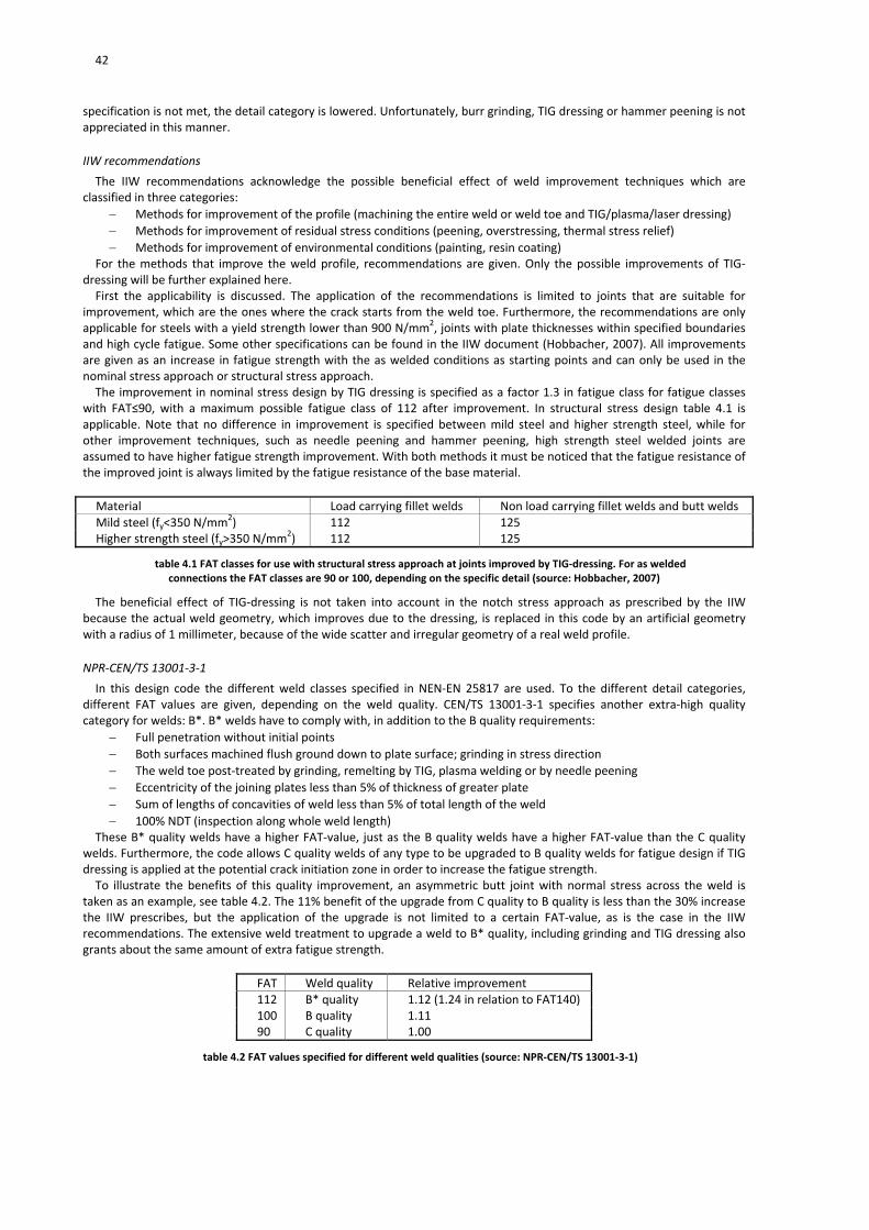
42
specification is not met, the detail category is lowered. Unfortunately, burr grinding, TIG dressing or hammer peening is not appreciated in this manner.
IIW recommendations
The IIW recommendations acknowledge the possible beneficial effect of weld improvement techniques which are classified in three categories:
Methods for improvement of the profile (machining the entire weld or weld toe and TIG/plasma/laser dressing)
Methods for improvement of residual stress conditions (peening, overstressing, thermal stress relief)
Methods for improvement of environmental conditions (painting, resin coating) For the methods that improve the weld profile, recommendations are given. Only the possible improvements of TIG‐
dressing will be further explained here. First the applicability is discussed. The application of the recommendations is limited to joints that are suitable for
improvement, which are the ones where the crack starts from the weld toe. Furthermore, the recommendations are only applicable for steels with a yield strength lower than 900 N/mm2, joints with plate thicknesses within specified boundaries and high cycle fatigue. Some other specifications can be found in the IIW document (Hobbacher, 2007). All improvements are given as an increase in fatigue strength with the as welded conditions as starting points and can only be used in the nominal stress approach or structural stress approach. The improvement in nominal stress design by TIG dressing is specified as a factor 1.3 in fatigue class for fatigue classes
with FAT≤90, with a maximum possible fatigue class of 112 after improvement. In structural stress design table 4.1 is applicable. Note that no difference in improvement is specified between mild steel and higher strength steel, while for other improvement techniques, such as needle peening and hammer peening, high strength steel welded joints are assumed to have higher fatigue strength improvement. With both methods it must be noticed that the fatigue resistance of the improved joint is always limited by the fatigue resistance of the base material.
Material Load carrying fillet welds Non load carrying fillet welds and butt welds Mild steel (fy<350 N/mm2) 112 125 Higher strength steel (fy>350 N/mm2) 112 125
table 4.1 FAT classes for use with structural stress approach at joints improved by TIG‐dressing. For as welded connections the FAT classes are 90 or 100, depending on the specific detail (source: Hobbacher, 2007)
The beneficial effect of TIG‐dressing is not taken into account in the notch stress approach as prescribed by the IIW because the actual weld geometry, which improves due to the dressing, is replaced in this code by an artificial geometry with a radius of 1 millimeter, because of the wide scatter and irregular geometry of a real weld profile.
NPR‐CEN/TS 13001‐3‐1
In this design code the different weld classes specified in NEN‐EN 25817 are used. To the different detail categories, different FAT values are given, depending on the weld quality. CEN/TS 13001‐3‐1 specifies another extra‐high quality category for welds: B*. B* welds have to comply with, in addition to the B quality requirements:
Full penetration without initial points
Both surfaces machined flush ground down to plate surface; grinding in stress direction
The weld toe post‐treated by grinding, remelting by TIG, plasma welding or by needle peening
Eccentricity of the joining plates less than 5% of thickness of greater plate
Sum of lengths of concavities of weld less than 5% of total length of the weld
100% NDT (inspection along whole weld length) These B* quality welds have a higher FAT‐value, just as the B quality welds have a higher FAT‐value than the C quality
welds. Furthermore, the code allows C quality welds of any type to be upgraded to B quality welds for fatigue design if TIG dressing is applied at the potential crack initiation zone in order to increase the fatigue strength. To illustrate the benefits of this quality improvement, an asymmetric butt joint with normal stress across the weld is
taken as an example, see table 4.2. The 11% benefit of the upgrade from C quality to B quality is less than the 30% increase the IIW prescribes, but the application of the upgrade is not limited to a certain FAT‐value, as is the case in the IIW recommendations. The extensive weld treatment to upgrade a weld to B* quality, including grinding and TIG dressing also grants about the same amount of extra fatigue strength.
FAT Weld quality Relative improvement 112 B* quality 1.12 (1.24 in relation to FAT140) 100 B quality 1.11 90 C quality 1.00
table 4.2 FAT values specified for different weld qualities (source: NPR‐CEN/TS 13001‐3‐1)

43
4.3.3 Influences of TIG‐dressing on material and geometry
Geometry
In the IIW recommendations on weld improvement techniques (Haagensen et al., 2001) detailed information is given on the TIG‐dressing progress and some global information is given on the geometrical result of the process. The torch position resulting in the optimum shape in theory and an actual specimen are depicted in figure 4.9.
figure 4.9 Effect of TIG‐dressing according to IIW recommendations (source: Haagensen et al., 2001)
The geometrical changes of TIG dressing can be quantified if the weld toe radius and weld toe angle are defined (see figure 4.10). The main effect of TIG dressing is the increase of the weld toe radius which results in a lower stress concentration at the weld toe. The weld toe angle remains approximately the same for fillet welds or butt welds with a cap that is high enough. For rather flat butt welds the angle will be reduced. The reduction of weld defects such as microcracks and small inclusions is more difficult to quantify, and is covered in the scatter of the results of most researches. In fact, the TIG dressing should reduce scatter by reducing the defects.
figure 4.10 Definition of weld toe radius and weld toe angle
Different authors have done research on the change of weld toe radius as a result of TIG dressing. Pedersen has collected a number of studies and has compared the weld toe radius of three weld improvement techniques with the as welded condition (Pedersen et al., 2010). His results are shown in figure 4.11. It is clear that a significant improvement in weld toe radius can be achieved by TIG dressing from an average of 1‐1.5 millimeter to an average of 6 millimeter. However, the variation of the radius also increases much compared with the as welded condition. Unfortunately it is not clear on which weld type these analyses are made, but context suggest the considered studies are mostly focused on fillet welds. This would also clarify the absence of measured weld toe angles.
figure 4.11 Comparison of toe radii in as welded and TIG dressed condition; the numbers between brackets refer to the sources of the graphs in the original article (source: Pedersen et al., 2010)
Residual stresses and microstructure
The additional weld process will have its influence on the residual stress distribution in the specimen, the microstructure and the associated hardness of the material in the (new) fusion zone and HAZ. A concern when TIG dressing is applied to high strength steel connections is the possibility of excessive softening of material (Pedersen et al., 2009). His investigation showed a hardness drop of 15% to 20% in the TIG dressed area.

44
A numerical analysis of the influence of TIG dressing on S690 base material has been made by Hildebrand (Hildebrand et al., 2006). His results show a strong increase in martensitic structure in the TIG dressed region where the previous state was mainly bainite. He also found a reduction in residual stress at the surface of the joint, while internally the area with high residual stressed increased. The results of the simulation for a butt joint are shown in figure 4.12.
figure 4.12 Microstructure and residual stress in simulated, TIG‐dressed butt joint (source: Hildebrand et al., 2006)
These results agree well with the research of Lopez Martinez (1997), where residual stresses where measured in actual specimens, before and after TIG‐dressing. The material that was used has a yield strength of 590 N/mm2 and a tensile strength of 757 N/mm2. He also found evidence that TIG‐dressing does not only influence the fatigue strength by geometrical modification of the joint, but also by lowering the residual stresses at the surface of the plates. The tests were executed on test specimens as shown in figure 4.13 . In figure 4.15 to figure 4.18 his findings are shown.
figure 4.13 Geometry of specimens tested by Martinez (source: Lopez Martinez et al., 1997)
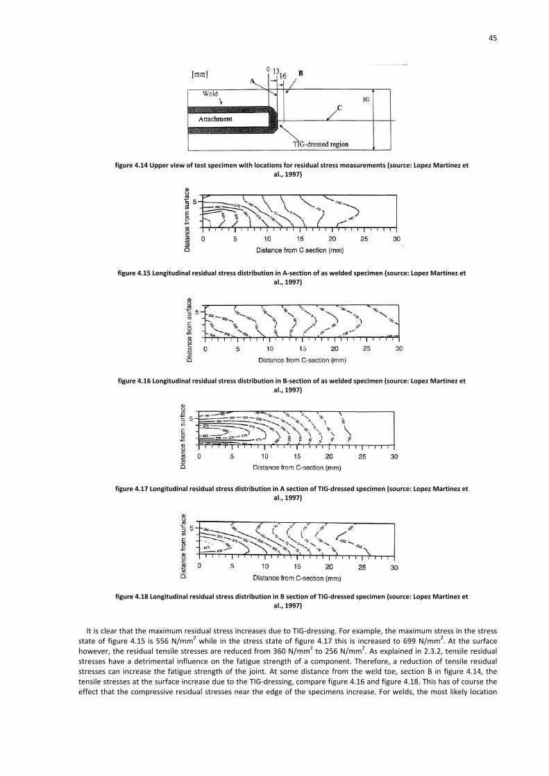
45
figure 4.14 Upper view of test specimen with locations for residual stress measurements (source: Lopez Martinez et al., 1997)
figure 4.15 Longitudinal residual stress distribution in A‐section of as welded specimen (source: Lopez Martinez et al., 1997)
figure 4.16 Longitudinal residual stress distribution in B‐section of as welded specimen (source: Lopez Martinez et al., 1997)
figure 4.17 Longitudinal residual stress distribution in A section of TIG‐dressed specimen (source: Lopez Martinez et al., 1997)
figure 4.18 Longitudinal residual stress distribution in B section of TIG‐dressed specimen (source: Lopez Martinez et al., 1997)
It is clear that the maximum residual stress increases due to TIG‐dressing. For example, the maximum stress in the stress
state of figure 4.15 is 556 N/mm2 while in the stress state of figure 4.17 this is increased to 699 N/mm2. At the surface however, the residual tensile stresses are reduced from 360 N/mm2 to 256 N/mm2. As explained in 2.3.2, tensile residual stresses have a detrimental influence on the fatigue strength of a component. Therefore, a reduction of tensile residual stresses can increase the fatigue strength of the joint. At some distance from the weld toe, section B in figure 4.14, the tensile stresses at the surface increase due to the TIG‐dressing, compare figure 4.16 and figure 4.18. This has of course the effect that the compressive residual stresses near the edge of the specimens increase. For welds, the most likely location
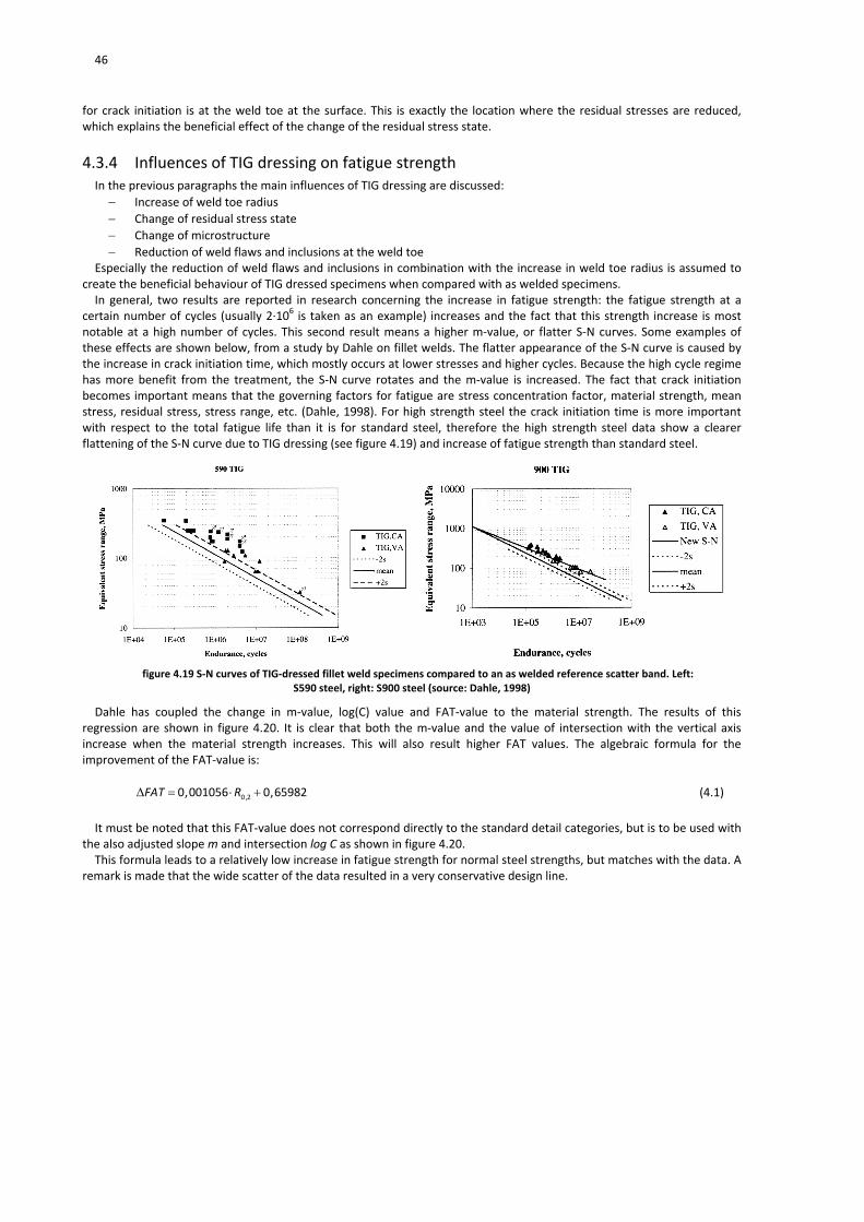
46
for crack initiation is at the weld toe at the surface. This is exactly the location where the residual stresses are reduced, which explains the beneficial effect of the change of the residual stress state.
4.3.4 Influences of TIG dressing on fatigue strength In the previous paragraphs the main influences of TIG dressing are discussed:
Increase of weld toe radius
Change of residual stress state
Change of microstructure
Reduction of weld flaws and inclusions at the weld toe Especially the reduction of weld flaws and inclusions in combination with the increase in weld toe radius is assumed to
create the beneficial behaviour of TIG dressed specimens when compared with as welded specimens. In general, two results are reported in research concerning the increase in fatigue strength: the fatigue strength at a
certain number of cycles (usually 2∙106 is taken as an example) increases and the fact that this strength increase is most notable at a high number of cycles. This second result means a higher m‐value, or flatter S‐N curves. Some examples of these effects are shown below, from a study by Dahle on fillet welds. The flatter appearance of the S‐N curve is caused by the increase in crack initiation time, which mostly occurs at lower stresses and higher cycles. Because the high cycle regime has more benefit from the treatment, the S‐N curve rotates and the m‐value is increased. The fact that crack initiation becomes important means that the governing factors for fatigue are stress concentration factor, material strength, mean stress, residual stress, stress range, etc. (Dahle, 1998). For high strength steel the crack initiation time is more important with respect to the total fatigue life than it is for standard steel, therefore the high strength steel data show a clearer flattening of the S‐N curve due to TIG dressing (see figure 4.19) and increase of fatigue strength than standard steel.
figure 4.19 S‐N curves of TIG‐dressed fillet weld specimens compared to an as welded reference scatter band. Left: S590 steel, right: S900 steel (source: Dahle, 1998)
Dahle has coupled the change in m‐value, log(C) value and FAT‐value to the material strength. The results of this regression are shown in figure 4.20. It is clear that both the m‐value and the value of intersection with the vertical axis increase when the material strength increases. This will also result higher FAT values. The algebraic formula for the improvement of the FAT‐value is:
0,20,001056 0,65982FAT R (4.1)
It must be noted that this FAT‐value does not correspond directly to the standard detail categories, but is to be used with
the also adjusted slope m and intersection log C as shown in figure 4.20. This formula leads to a relatively low increase in fatigue strength for normal steel strengths, but matches with the data. A
remark is made that the wide scatter of the data resulted in a very conservative design line.

47
figure 4.20 Influence of material strength on S‐N curve parameters. Left: m and C. Right: FAT‐value. (source: Dahle, 1998)
Dahle also calculated the increase in fatigue strength of the individual data points with respect to the reference scattering band. In table 4.3 the average outcomes of this calculation are shown per steel grade. It is clear that the material strength has an influence on the beneficial effect from TIG dressing. Both data from constant amplitude loading and variable amplitude loading are incorporated in the calculation.
Steel Grade Yield strength [N/mm2] Average improvement of fatigue strength 350 398 1.185 590 615 1.424 700 780 1.725 900 900 1.894
table 4.3 Increase in fatigue strength (source: Dahle, 1998)
Similar results arise from the research of Pedersen et al. (2009), where the free slope of the fatigue curve of TIG‐dressed S700 grade specimens increases to 5.9 compared to 4.2 for as welded specimens of mixed steel grade. The reported beneficial effect at 105 cycles is around 38% and around 70% at 2∙106. This research also considers fillet welds only More research on the beneficial effect of TIG dressing on fillet welds has been done by Huo (2005). This research does
not focus on high strength steel but distinguishes results for constant amplitude loading and variable amplitude loading. The results, comparing two post weld treatments to the as welded condition, are shown in figure 4.21. The test data show much less scatter than the low strength data of Dahle, which leads to a greater increase of the fatigue strength: approximately 37% for steel with σy=390 N/mm2.
figure 4.21 Comparison of two weld improvement techniques with the as welded situation for a steel with a yield limit of 390 N/mm
2 and a tensile strength of 590 N/mm
2. Tested on fillet weld specimens (source: Huo et al., 2005)
The effects discussed by Dahle are partially visible in the data published by Huo. If only the constant amplitude (CA) data published by Huo are considered it is clear that the fatigue strength of the connection increases, but the higher m‐value is barely visible. This might be due to the fact that the steel in question is of standard quality, while the flattening effect in the study of Dahle was most notable for higher strength steels.

48
Other results are published by Haagensen, who found an average increase of 44% in the fatigue strength of a fillet weld joint, but no change in slope of the S‐N curve (Haagensen et al., 1987). This result was also found for standard steel with a yield strength of 365 N/mm2, which means it does not exclude the flattening effect for higher strength steels. All research shows an increase in fatigue strength of TIG dressed specimens. The increase in fatigue strength differs from
20% to 40% for standard steels and can be as high as 90% for very high strength steels. The research data by Dahle and Pedersen also shows a rotation of the S‐N curve, especially for high strength steels in the case of Dahle. Other researches do not show this effect, but also do not incorporate high strength steels, so they do not confirm nor refute the presence of this effect. All discussed researches consider fillet welds only. Whether the effect will be similar on butt welds shall have to show from this testing programme.

49
5 Test setup
5.1 Chapter outline In this chapter the testing programme and test setup are discussed. In paragraph 5.2, the identification, dimensions and
fabrication of the specimens is discussed. The test setups that have been used for the different experiments are shown and explained in paragraph 5.3.
5.2 Testing programme
5.2.1 Identification of test specimens In total there were 11 plates available for testing, each with different specifications. The specimens indicated by a V
consist of two rolled plates connected by a V‐butt weld. The specimens indicated by a C consist of a rolled plate and a cast plate of similar static strength, connected by a V‐butt weld. The cast steel plate is in general slightly thicker (about 5%) than the rolled steel plate. The number in the specimen identification code refers to the first two numbers of its steel grade. The available plates are:
Plates V89, V46, V69, C69 and C46 with approximate dimensions 330 x 25 x 950 mm3.
Plates C11 and V11 with approximate dimensions 330 x 20 x 950 mm3.
Plate C89 with approximate dimensions 320 x 25 x 950 mm3, with a longitudinal cut along the full length except for the weld area.
Plate C89a with approximate dimensions 160 x 25 x 950 mm3. With the available material 24 strips with a width of approximately 100 millimeter were produced for fatigue testing.
Each plate, except C89 and C89a, is therefore divided in three pieces of approximately 100 millimeter and one ±25 millimeter residual strip which can be used for hardness measurements. The C89 plate is divided in two specimens and the third C89 specimen is produced from plate C89a. The produced specimens are shown in Annex B in tabulated form. The material specifications can be found in the material certificates provided in Annex D.
5.2.2 Preparation of specimens The specimens were prepared according to IIW recommendations on TIG dressing (Haagensen et al., 2001). Both the cap
and root sides of the V‐butt weld were TIG dressed. To provide a suitable geometry on which to apply TIG dressing, the weld root was ground off until a limited height remained. The weld roots of two specimens could not be TIG dressed:
C69. After grinding the weld root, small porosities were visible. To prevent these gas inclusions swelling up during the TIG dressing process, resulting in an unsatisfactory end result, this root was not TIG dressed. It would be interesting to investigate whether these gas inclusions would indeed have spoiled the TIG dressing process, whether these inclusions would show up on an X‐ray test and whether they would pass or fail this test. Depending on the answers on these questions these porosities could have serious consequences for the practical application of the TIG dressing process.
C89. This plate consists of 2 butt welded specimens joined together longitudinally. One half of the plate had insufficient weld height to prevent the TIG dressing process causing undercut. Therefore, this half was not TIG dressed on the weld root.
In both these cases only the weld toes at the weld cap were TIG dressed. Because the misalignment due to welding will cause extra tensile stresses at the weld cap when the fatigue tests commence, the fatigue cracks are expected to initiate there. Therefore the decision not to TIG dress the weld roots will probably not have any influence on the outcome of the tests. All plates were flame cut into strips of approximately 100 millimeter in width. Subsequently a reduction in cross section
was made near the weld to prevent fatigue cracks in the parent material near or in the clamps of the testing rig. The final dimensions of all specimens are depicted in Annex B.

50
5.3 Test setup
5.3.1 Measurement of weld geometry To make an accurate measurement of the weld geometry a sensor has been mounted to an X‐Y motor. This laser sensor
measures the distance from its own position to the object that is to be scanned. An overview of the measuring setup is shown in figure 5.1.
figure 5.1 Setup to measure the geometry of welds
The X‐Y motor has a precision of 1/160 millimeter in both directions. The laser sensor has a resolution of 1/1000 millimeter over its full bandwidth which can be increased by sample averaging to 1/10000 millimeter. An overview of the type of laser sensor that has been used is shown in figure 5.2.
figure 5.2 Type of laser sensor used in measuring the weld geometry
Silicon rubber casts
To speed up the total process of measuring and preparation of the specimens and to make the changing of specimens more manageable, silicon rubber casts were made of the welds. The casts are an exact negative reproduction of the weld. The specifications of the used silicon rubber can be found in the manufacturer’s website. The used rubber is of the type PS81020 from Polyservice in The Netherlands. In figure 5.3, laboratory staff is casting the silicon rubber onto the steel plates. The result of the casting is shown in figure 5.4.

51
figure 5.3 Casting of the silicon rubber onto the steel plates
figure 5.4 Silicon rubber cast of C89a plate
5.3.2 Measurement of fatigue life The prepared specimens are tested under axial loading in the Stevin Laboratory of the Delft University of Technology. The
used test rig is depicted in figure 5.5. The testing rig has a maximum load of 600 kN.
figure 5.5 Schematic of testing rig (image source: Pijpers, 2011)

52
The starting point of each measurement is the unclamped, unloaded specimen. This means that the deformation arising from the static clamping of the imperfect specimens already results in non‐zero measured tensile strains at the weld cap. For all specimens the intention is to test at R=0.1, but due to the aforementioned tensile strains and the resulting
stresses, this requires the minimum load to be a compression load in many cases. This is deemed unpractical, and possibly unsafe, therefore a minimal tensile load of 10 kN is taken as a lower bound for the minimum load. The actual R‐value is documented, based on both the strain gauges and the measured force. Twelve strain gauges were placed on each specimen. The location of the strain gauges and global dimensions of the
specimens are depicted in figure 5.6. The numbering of the strain gauges is depicted in Annex B.
figure 5.6 Global dimensions of specimen and location of strain gauges
Crack monitoring
When one of the strain gauges starts showing a strain range which deflects significantly from its average, the system shuts down the test rig so that, when restarted, crack monitoring can take place. When the crack occurs near one of the strain gauges it can be detected at a crack length of about 10 millimeter. If the crack occurs further away, the crack length at detection can be much longer, up to 40 millimeter. Cracks are monitored in two ways. To visualize the crack, some petroleum is brushed onto the surface of the specimen
and subsequently wiped away. The length of the crack at the surface can then directly be measured with a vernier caliper. This measurement can be executed relatively frequent. Another method to monitor cracks is crack marking. This involves raising the lower stress in the specimen to about 90%
of the upper stress in the specimen, thereby greatly reducing the stress range, for 2% to 10% of the expected total number of cycles to failure. This results in visible ‘beach marks’ on the crack surface after failure of the specimen. Because the stress range is much lower during this procedure, the number of stress cycles made in this procedure can be neglected in the total amount of stress cycles before failure. A good example of the result of crack marking is shown in figure 5.7, but not all specimens give the good results as shown in the image. Some specimens fail rather quick after crack initiation, thus allowing only two or three crack markings. In other specimens, while the crack marking was executed more often, none or not all marks are visible. In general, crack marking cannot be executed as frequently as the surface measurement, because the markings must have some distance in between each other, preferable a few millimeters. Furthermore, the assumption that the number of cycles during marking can be neglected will become dubious if crack marking is executed to frequently.
figure 5.7 Beach marks visible in a specimen
5.3.3 Measurement of material hardness Of all plates a small piece of material has been polished and etched to distinguish the weld material, heat affected zone
and parent material. On the different zones hardness measurements have been carried out. This is a standardized test and is executed according to the applying codes. For more details on the testing, reference is made to Annex H. The results are discussed in 7.4.

53
6 Processing and results of laser measurements
6.1 Chapter outline In this chapter the results of the laser measurements are discussed. In paragraph 6.2 is discussed how the raw data is
processed to usable results. Any issues that were encountered are discussed and a solution is presented. The distribution of the weld toe parameters and any differences between cast and rolled steels or different steel strengths are discussed in paragraph 6.3.
6.2 Test output and processing laser measurements
6.2.1 Test output The direct output from the laser scan is a table containing the position of the laser and the measured distance. For post
processing the laser position and measured distance are separated and the measured data are leveled out by subtracting a plane from the data in such a way that the parent plate has value 0. The matlab scripts to perform these actions, and all coming processing actions are shown in Annex F. Now the first results can be plotted in 3D, as shown in figure 6.1 and figure 6.2.
figure 6.1 3D overview of a the weld of plate V46 before TIG dressing, no gridlines are shown to keep the image clear

54
figure 6.2 Zoomed in on figure 6.1, with gridlines at a 0.05x0.5 mm2 grid
From the same datasets weld cross sections can be plotted (see figure 6.3), which can be used to determine the geometry of the weld toe.
figure 6.3 Cross section of the weld of plate V46. Axes are in millimeters.
Four characteristic values have been chosen to describe the weld toe: 1. Weld toe radius 2. Weld toe angle 3. Weld height 4. Undercut
In figure 6.4 these characteristic values are shown on a fictive, exaggerated weld toe cross section.

55
figure 6.4 Possible measured weld profile (exaggerated) and its accompanying schematization
6.2.2 Determining the weld radius The radius is measured by creating a fine grid around an estimated midpoint for the circle which coincides with the notch
root. For each grid point the distance to each data point of the weld geometry is calculated over a user specified section. The grid point that shows the least variation in these distances is the best suitable midpoint and the accompanying weld toe radius is determined by averaging all distances. The script of this process is shown in Annex F. Some steps of the process are shown in figure 6.3 and figure 6.5.
figure 6.5 Optimized circle for the left weld toe (red) of the same weld cross section as shown in figure 6.3. The optimal midpoint is marked. Axes are in millimeters
Unfortunately, the process is not completely automatic. The user must specify the boundaries of the grid by specifying an expected circle midpoint and the grid width and height. If this is not done properly the optimized midpoint will lie at the edge of the grid, because the actual optimal midpoint lies outside the gird. In this case the user can specify a larger grid or relocate the expected midpoint until the optimized midpoint lies at a satisfactory distance from the edge of the grid. The user must also specify boundaries between which the circle must be optimized. In figure 6.5 these boundaries are chosen as 5.25 millimeter and 5.75 millimeter. Of course these boundaries are estimates and could also be estimated at slightly different values. In figure 6.6 a plot is shown where the optimization boundaries where varied to a certain extent.

56
figure 6.6 Different radii for different optimisation boundaries. Axes are in millimeters.
In figure 6.6 different circles are shown as the result of different optimization boundaries. Unfortunately, there is no absolute way of determining which circle is the best optimization. An obvious indication of the best circle is the variation in the distances from its midpoint to the data points: the circle for which the total variation is the least fits the weld geometry the best. However, because the number of data points is reduced when the optimization boundaries are narrowed, it is easier for the program to make a better optimization. Therefore, narrower optimization boundaries will always result in a lower variation. From figure 6.6 can be concluded that rather large differences in weld toe radius can be found if the optimization boundaries are varied. The boundaries and their accompanying radii as drawn in figure 6.6 are shown in table 6.1.
Optimisation boundaries [mm] Radius [mm] 5.15 – 5.85 1.61 5.20 – 5.80 1.40 5.25 – 5.75 1.20 5.30 – 5.70 1.24 5.35 – 5.65 1.04 5.40 – 5.60 0.74
table 6.1 Different determined radii for different optimisation boundaries
From figure 6.6 cannot clearly be concluded which of the circles fits best. If a zoomed in version of figure 6.6 is considered (figure 6.7) it is clear that the circle with the smallest radius (0.74 millimeter) is too pessimistic. The circle with the largest radius is too optimistic, especially on the right side of the figure. To the eye, the circles with radii 1.20, 1.24 and 1.40 millimeter seem to match best with the weld.

57
figure 6.7 Zoomed in on figure 6.6. Axes are in millimeters.
Another remark must be made on the small dimple in the weld geometry that can be seen around 5.55 on the horizontal axis of figure 6.7. This could also be regarded as a very small notch, with a very small radius. These types of dimples or other irregularities that could be interpreted as a small notch occur in a large number of weld cross sections, both as welded and TIG‐dressed. A choice must be made to either use the large radius or use the small radii as characteristic value. The following sections will first address the possible subjectivity of the determination of the radii and ways to make it as
objective as possible. Then the issues concerning the additional smaller radii will be discussed.
Choosing the ‘correct’ radius for the weld toe
As described above, the determining of the weld toe radius cannot be done entirely automatic. The user of the program influences the outcome to a certain extent. To determine whether the found weld toe radius is acceptable, a number of checks can be made:
1. Where the found radius intersects or meets the measured weld profile, the tangent of the circle must coincide with the tangent of the measured weld profile.
2. When the boundaries are varied a small amount, the found radii must not greatly differ from each other. For example, the three radii in figure 6.7 which are deemed to fit rather well, are all determined with different boundaries but do not differ greatly. However, if the boundaries of the smallest circle are slightly enlarged the radius varies greatly. In this case, the smallest circle is influenced too much by the small dimple in the measured weld profile.
3. The overall image must be satisfactory. This is of course extremely subjective, but is one of the most important tools to judge a radius. For example: for the program it is very difficult to filter out the small dimple in the middle of figure 6.7, but a person can easily see that, if the large radius has to be determined, the small dimple can be ignored.
To get an estimate of the amount of subjectivity involved in the process, the analysis process has been carried out twice for one weld cast. The results of this are shown in table 6.2. It is clear that the differences in mean and standard deviation are very small. The differences in mean value can even be neglected when the size of the standard deviation is taken into account.
Radius Angle
Measurement 1 2 1 2
Mean [mm] 1.26 1.28 25.64 24.98
Standard Deviation [mm] 1.12 1.02 5.40 5.07
table 6.2 Comparison of measured weld radii and angle for two different measurements of the same weld profile
This test does not prove that the weld profile measurements are fully objective, but can be used as an indication of the amount of variation to be expected in the weld toe parameters by the user input in the program.

58
Choosing between large and small radius
In figure 6.7 two radii can be seen, a large one, for which the circles are drawn, and a smaller dimple in the middle of the figure. Both these radii could be used to determine the ‘characteristic radius’ for this weld toe profile. This problem is not unique for the weld profile shown in the figure, but occurs regularly. To solve the problem, experts on welding and fatigue at the faculty of mechanical engineering of Delft University of
Technology were consulted. A suggestion was made that the small radius might be too small to have influence on the crack initiation of the specimen. In fracture mechanics this problem is addressed with the Kitagawa‐Takahashi diagram (Janssen et al., 2002). This diagram describes the influence of a surface imperfection on the fatigue limit of the specimen. On the horizontal axis the size of the imperfection (a) is shown, which in this case is the depth of the small radius in relation to a ‘smooth’ larger radius. On the vertical axis the threshold stress range to initiate a crack in plain material is shown (σth). The diagram is build of out of two lines, one describing the fatigue limit, and one line depending on the threshold value of K, as used in fracture mechanics (see 3.4). In the example of figure 6.8 the threshold stress to initiate a crack lies around 350 N/mm2 for small defects. When defects increase to a size greater than a certain value, the threshold stress will start to decline. As a rule of thumb we can state that below the intersection point of the two dotted lines, l0, the threshold stress does not decline by a large amount. This means that if a small defect (the small radius) is smaller than l0 it will not influence the minimal stress to initiate a crack, and will therefore not influence the fatigue life.
figure 6.8 Example of a Kitagawa‐Takahashi diagram for a nodular cast iron (Δσe = 320 MPa ΔKth=6.2 MPa√m) (source: Janssen et al., 2002)
To determine whether the small radii have to be taken into account, first l0 has to be determined for the different materials. When both σe and ΔKth are known, the value of l0 can be determined. To quickly assess the influence of the small radii not all materials are considered, but a selection of two materials is made: S690 and S1100. It is especially important that S1100 is considered because previous research (Pijpers, 2011) has shown that these specimens are very sensitive for surface roughness. For the endurable stress range in plain material (σth=σE) reference is made to experiments carried out on this material
(Pijpers, 2011). On plain specimens, with mill skin in place, tests were performed. For both materials a runout was found below a certain stress. This stress will here be used as σE. The values of the used fatigue limits are given in table 6.3.
Material σE [N/mm2]
S690 270
S1100 378
table 6.3 Endurable stresses on plain material
Different authors have reported on the value of ΔKth. The different recommendations are shown in table 6.4. A remark must be made on the recommendation of the IIW (Hobbacher, 2007), in which for very small surface cracks it is reported that the Kth may be lower than specified in table 6.4. However, based on the experiences of all other authors, where no such remark is made, a value of 63 Nmm‐3/2 is assumed to be sufficiently conservative.

59
ΔKth [Nmm‐3/2] author
101 up to 120 Wanhill, 1991
102.2 up to 208.7 Romeijn, 2006
240‐173∙R Gruney, 1979
170‐214∙R≥63 Hobbacher, 2007
table 6.4 Different estimates of ΔKth
With these data the value of l0 can be determined. For a limited number of weld cross sections an analysis is made of the depth of the ‘small radius’ if one is present. The results of this, and the calculated l0 are shown in table 6.5. It is clear that most radii lie around the value of l0 (note that the Kitagawa‐Takahashi diagram uses log‐scales on both axes). The small radii may therefore have an influence on the fatigue strength of that local material, but as this influence is relatively small it can probably be ignored, especially when it is taken into account that for ΔKth values can occur which significantly increase the value of l0.
V11 V69
x [mm] toe radius [mm] depth of 'small radius' [mm] x[mm] toe radius [mm] depth of 'small radius' [mm]
30 4.5732 0.0255 30 0.9837 0.0086
60 0.1614 N/A 60 0.8090 0.0149
90 1.7606 0.0189 90 1.7725 0.0287
120 2.7126 0.0171 120 0.3471 N/A
150 0.9171 0.0086 150 0.5420 0.0056
180 1.3947 N/A 180 0.2387 N/A
210 2.2831 0.0088 210 0.5109 N/A
240 1.7988 0.0047 240 1.1260 N/A
270 1.0579 0.0066 270 1.7184 0.0227
300 0.6709 N/A 300 2.0000 0.0187
330 3.6710 0.0381 330 0.4925 N/A
Mean 1.9092 0.0160 Mean 0.9583 0.0165
Stdev 1.3260 0.0114 Stdev 0.6212 0.0086
l0 0.0088 l0 0.0173
table 6.5 Analysis of occurring small radii and their depth in relation to a 'smooth' curve
Furthermore, these smaller radii occur mostly at some distance into the weld, where the maximum stress peak is not located, and therefore suffers from a lower stress range. As a final argument to choose the larger radius as characteristic, is the fact that the smaller radii occur both in the as
welded specimens and TIG‐dressed specimens, with comparable regularity. Therefore, the large radius is the changing factor and thus interesting to record.
6.2.3 Determining the weld toe angle, weld height and undercut For the determination of these tree values a platform of straight parent material is used as base value. From this base the
angle, height or undercut at the weld toe can be determined. To save time, the measurements only incorporate a limited distance of parent material (a few millimeters). This sometimes leads to difficulties because undercuts cannot always be distinguished from the straight parent material. If additional research is done on this topic, a wider measurement scope is highly recommended. About 10 millimeter of parent material, measured from the weld toe, will probably suffice. It might be possible to increase the across‐the‐weld grid size at distances greater than a few millimeters from the weld toe, to keep the measuring time within limits.
6.3 Results
6.3.1 Observed geometries The analysis of weld geometries has resulted in around 750 radii, angles and undercuts and about 375 weld heights for
both the as welded condition and the TIG‐dressed condition. The as welded geometries all looked very similar, but the TIG‐dressed geometries showed four characteristic shapes, which all appeared in different regularity. The global shape of the observed weld toe shapes for both the as welded and TIG‐dressed condition are shown in figure 6.9.

60
figure 6.9 Observed weld toe shapes (fictive geometries, for communication purposes)
Typical As welded. The as welded specimens generally have, to the eye, the same geometry. The parent material shows no great undercuts. Then the weld material starts after a relatively small radius. The angle of the weld material is rather steep.
Typical TIG‐dressed, Type 1. This is the desired effect of TIG dressing (see 4.3.3, especially figure 4.9). The overall weld geometry is much smoother. The weld radius is much larger than in the as welded state, and the weld toe angle is reduced.
Typical TIG‐dressed, Type 2. A significant undercut is visible, even to the naked eye on the weld itself. The undercut has depths up to about 0.5 millimeter. The weld toe radius is generally larger than observed in Type 1, and the weld toe angle somewhat steeper than for Type 1. Type 2 does occur, but not very frequently, and also not in every weld.
Typical TIG‐dressed, Type 3. To the eye this looks very similar to Type 1. However, a small ridge can be felt with a sharp object or the fingernail. It seems the weld has solidified before an entirely smooth geometry was formed. In the measurements, the radius and angle of the first, and in all cases smallest, radius was measured. The weld angle of this type is similar to the weld angle of Type 1. Type 3 occurs rather frequently, and can be found in most, if not all studied welds.
Typical TIG‐dressed, Type 4. A small weld toe radius followed by a rather steep angle (similar to as welded) for a very short distance. After this, the angle declines back to similar values as found in Type 1 and Type 3. Type 4 occurs far less frequent than Type 1 and Type 3.
It would be very interesting to make an inventory of the exact frequency of the different types, which could be matched
to fabricating conditions (experience of the welder, heat input, etc.) and to the point of crack initiation. Furthermore, it would be very interesting to investigate the existence and frequency of these typical geometries in TIG‐dressed welds in practice. The welds studied in this research were all TIG‐dressed by the same welder, under the same conditions on the same day. Furthermore, all considered weld cross sections are taken from a very limited number of welds, which could influence the results.
6.3.2 Comparison between rolled and cast steel All data have been gathered and can be split in TIG‐dressed and as welded or rolled and cast steels. It is visible to the eye
that TIG‐dressing has had great influence on the weld geometry. Whether there is a clear difference between rolled and cast steels has to result from the data from the weld geometry measurements. Only the parameters weld toe radius, weld toe angle and undercut will be compared, because the weld height is deemed independent from the parent material, especially since cast plates are always welded to a rolled plate in this research.

61
Weld toe radii
Bar diagrams of the density of measured radii for both rolled and cast steel are shown in figure 6.10. An overlay of these two diagrams is shown in figure 6.11. It is clear that the cast steel radii show a sharper peak, in contrast with the smoother diagram shown by the rolled steel data. The location of the peaks of both diagrams shows no large difference, especially when the spread of the data is taken into account.
figure 6.10 Comparison of as welded radii between rolled steel and cast steel [mm]
figure 6.11 Overlay of as welded radii; cast (―) and rolled (‐ ‐ ‐) steel [mm]

62
Density bar diagrams for TIG‐dressed radii are depicted in figure 6.12 with an overlay in figure 6.13. The radii of the rolled steel show a density peak roughly at the same location as the cast steel and an additional peak of smaller radii. This can be a significant difference, but can also arise from the fact that all data result from a limited number of welds. One weld bead that has a lower quality, can easily influence the results to an extent that the differences between the two figures can be explained. Aside from the additional peak the global shape of the diagrams appears roughly the same.
figure 6.12 Comparison of TIG‐dressed radii between rolled steel and cast steel [mm]
figure 6.13 Overlay of TIG‐dressed radii of cast (―) and rolled (‐ ‐ ‐) steel [mm]

63
Weld toe angles
In figure 6.14 density bar diagrams are shown for the weld toe angles of as welded specimens. An overlay of both diagrams is shown in figure 6.15. It is clear that the diagrams are very similar.
figure 6.14 Comparison of as welded angles between rolled steel and cast steel
figure 6.15 Overlay of as welded angles of cast (―) and rolled (‐ ‐ ‐) steel

64
In figure 6.16 density bar diagrams are shown for weld toe angles of TIG dressed specimens. An overlay is shown in figure 6.17. The peak of both data samples differs, but when the spread of the data is taken into account, it is questionable whether this is a significant difference.
figure 6.16 Comparison of TIG‐dressed angles between rolled steel and cast steel
figure 6.17 Overlay of TIG‐dressed angles of cast (―) and rolled (‐ ‐ ‐) steel
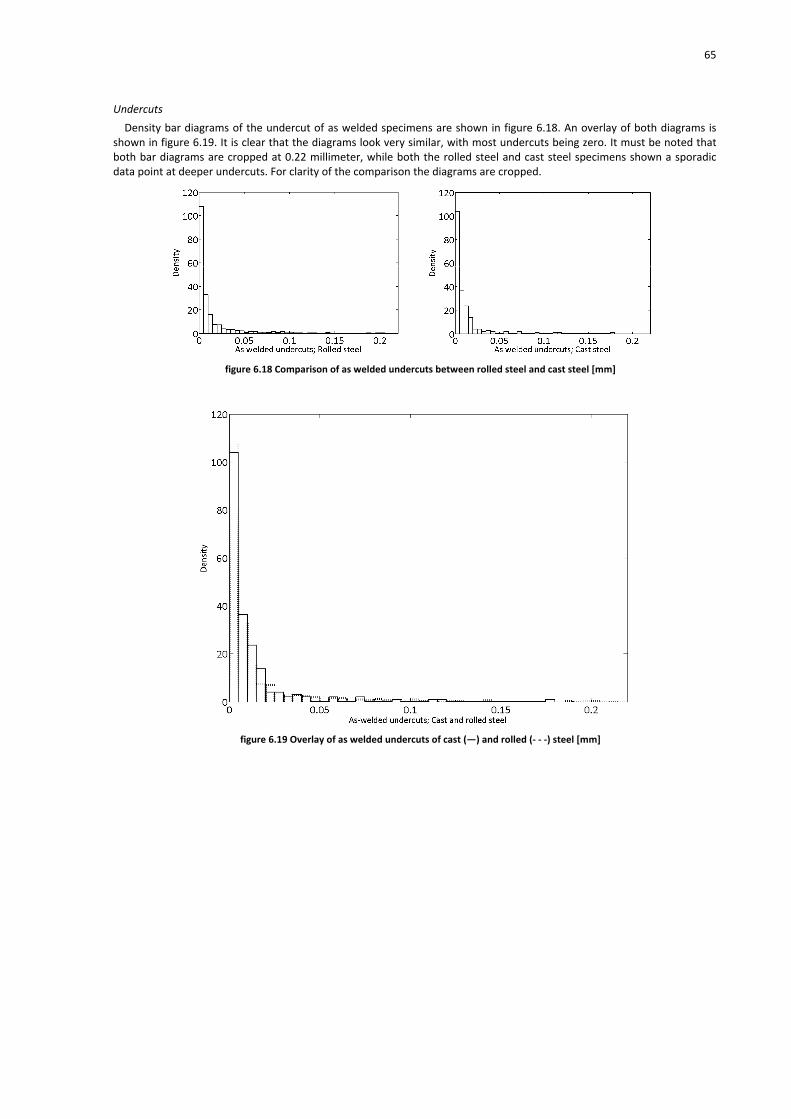
65
Undercuts
Density bar diagrams of the undercut of as welded specimens are shown in figure 6.18. An overlay of both diagrams is shown in figure 6.19. It is clear that the diagrams look very similar, with most undercuts being zero. It must be noted that both bar diagrams are cropped at 0.22 millimeter, while both the rolled steel and cast steel specimens shown a sporadic data point at deeper undercuts. For clarity of the comparison the diagrams are cropped.
figure 6.18 Comparison of as welded undercuts between rolled steel and cast steel [mm]
figure 6.19 Overlay of as welded undercuts of cast (―) and rolled (‐ ‐ ‐) steel [mm]

66
The density bar diagrams of the undercuts of TIG‐dressed specimens are shown in figure 6.20. An overlay of both diagrams is shown in figure 6.21. For small undercuts both diagrams show similar behaviour, but for deeper undercuts, the cast steel specimens show much more undercuts. This can attributed to the fact that the large majority of typical TIG‐dressed type 2 weld geometries (see figure 6.9) occurred in one weld in the C69TIG plate on the cast side.
figure 6.20 Comparison of TIG‐dressed undercuts between rolled steel and cast steel [mm]
figure 6.21 Overlay of TIG‐dressed undercuts of cast (―) and rolled (‐ ‐ ‐) steel [mm]
Conclusion
The overlay diagrams of the weld toe radii, weld toe angles and undercuts show different results. In some cases the results match almost exactly, and in some cases the cast and rolled steels show rather different results. Before a conclusion can be drawn, a few factors must be considered. First of all, the data set for cast steels is much smaller than for the rolled steels, since all cast steel plates are welded to a
rolled steel plate. This results in a roughly three times larger data set for the rolled specimens. This could explain some of the sharp peaks the cast steel data show (e.g. see figure 6.11). Furthermore it must be noted that all data result from only nine welds in total, which in turn may be built up from multiple weld beads. This means that in total only eighteen weld beads have been measured (one for each weld toe). If one of those weld beads has been fabricated in a less than perfect way, this can very easily translate into large differences in the above analysis. For example, the large majority of large undercuts that are visible in cast steel appear in the C69TIG plate. Based on these considerations and the fact that the differences between peaks generally do not exceed the standard
deviation, it is assumed that the welds in cast steel and rolled steel have similar distributions of geometry.

67
6.3.3 Comparison between different steel grades The data sets of the individual measured plates consist of relatively few data points. This will result in very rough bar
diagrams. This effect was already noted in 6.3.2 where the rolled and cast measurements were compared. In this case there is not a difference in data size, but the small size of the data set severely distorts the overlay of two bar diagrams. Therefore, in this paragraph only mean values and standard deviations will be compared. The results for weld height are not taken into account, because this differs greatly between plates, and mainly depends on the skill of the welder and the amount of added weld material. In table 6.6 to table 6.8 the comparison between the different materials can be made, both for the as welded as TIG‐dressed situation. For the weld toe radius and weld toe angle hardly any differences can be observed, and any differences are small when compared with the standard deviation. For the undercut in the as welded situation there seems to be a material dependent influence, but as this influence is not apparent in the TIG‐dressed situation it is concluded that the steel grade has no influence on the weld toe parameters.
As welded TIG‐dressed
mean [mm] stdev [mm] mean [mm] stdev [mm]
S1100 1.4188 1.0184 4.5360 2.9817
S890 1.5691 0.9458 4.9847 4.4375
S690 1.5210 1.1274 4.5058 3.1078
S460 1.8761 1.6850 3.6718 3.2851
table 6.6 Comparison of mean value and standard deviation of weld toe radii. The given values are also applicable to the cast steel counterpart of the mentioned rolled steels.
As welded TIG‐dressed
mean [‐] stdev [‐] mean [‐] stdev [‐]
S1100 29.0235 5.9754 14.5088 4.2531
S890 28.3556 5.5604 14.1985 4.8029
S690 27.9500 6.2554 17.0907 6.0301
S460 26.0104 7.9736 15.7443 3.7348
table 6.7 Comparison of mean value and standard deviation of weld toe angles. The given values are also applicable to the cast steel counterpart of the mentioned rolled steels.
As welded TIG‐dressed
mean [mm] stdev [mm] mean [mm] stdev [mm]
S1100 0.0217 0.0534 0.0231 0.0369
S890 0.0176 0.0352 0.0161 0.0314
S690 0.0077 0.0120 0.0368 0.0850
S460 0.0067 0.0102 0.0142 0.0151
table 6.8 Comparison of mean value and standard deviation of undercuts. The given values are also applicable to the cast steel counterpart of the mentioned rolled steels.
6.3.4 Distribution of weld geometry parameters Based on the previous paragraphs, the data for cast and rolled steel or different steel grades will not be analyzed
separately. In this paragraph collected data of all weld geometry parameters will be plotted.
Weld toe radius
In figure 6.22 the results of the laser measurements are shown for as welded and TIG‐dressed specimens. An overlay of both diagrams is shown in figure 6.23. The overall trend is what is to be expected from TIG‐dressing: the weld toe radius increases. However, very small radii still occur and their numbers are still significant. This will be due to the occurrence of typical TIG‐dressed geometries type 3 and 4 (see figure 6.9). The spread of the TIG‐dressed radii is much larger than for the as welded radii with the occurrence of the aforementioned small radii, but also very large radii occur. A tabulated summary of the results is given in table 6.9. Note that the values of the weld toe radii are not normally distributed. The values in table 6.9 should therefore not be used as such.

68
figure 6.22 Comparison of as welded and TIG‐dressed radii [mm]
figure 6.23 Overlay radii of as welded (―) and TIG‐dressed (‐ ‐ ‐) specimens [mm]
Mean [mm] Standard dev. [mm]
As welded 1.5940 1.2256
TIG‐dressed 4.6807 3.5462
table 6.9 Mean and standard deviation of measured radii
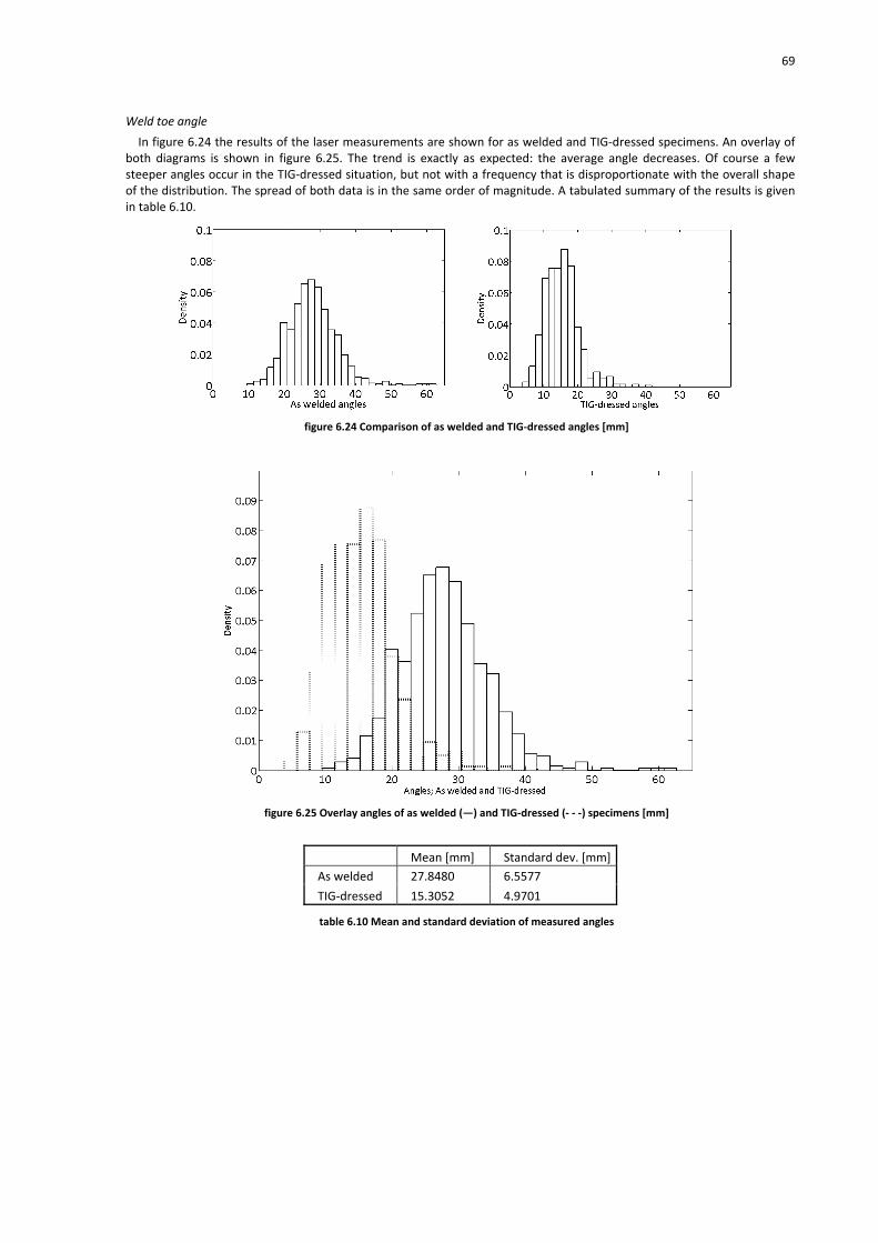
69
Weld toe angle
In figure 6.24 the results of the laser measurements are shown for as welded and TIG‐dressed specimens. An overlay of both diagrams is shown in figure 6.25. The trend is exactly as expected: the average angle decreases. Of course a few steeper angles occur in the TIG‐dressed situation, but not with a frequency that is disproportionate with the overall shape of the distribution. The spread of both data is in the same order of magnitude. A tabulated summary of the results is given in table 6.10.
figure 6.24 Comparison of as welded and TIG‐dressed angles [mm]
figure 6.25 Overlay angles of as welded (―) and TIG‐dressed (‐ ‐ ‐) specimens [mm]
Mean [mm] Standard dev. [mm]
As welded 27.8480 6.5577
TIG‐dressed 15.3052 4.9701
table 6.10 Mean and standard deviation of measured angles

70
Undercut
In figure 6.26 the results of the laser measurements are shown for as welded and TIG‐dressed specimens. An overlay of both diagrams is shown in figure 6.27. The diagrams show a slight increase in non zero undercuts for TIG‐dressed specimens, but both TIG‐dressed and as welded specimens have hardly any undercuts larger than 0.05‐0.1 millimeter. The TIG‐dressed specimens contain a few deeper undercuts as described above. A tabulated summary of the results is given in table 6.11.
figure 6.26 Comparison of as welded and TIG‐dressed undercuts [mm]
figure 6.27 angles of as welded (―) and TIG‐dressed (‐ ‐ ‐) specimens [mm]
Mean [mm] Standard dev. [mm]
As welded 0.0136 0.0335
TIG‐dressed 0.0229 0.0512
table 6.11 Mean and standard deviation of measured undercuts

71
Weld height
Because TIG‐dressing takes place at the weld toe, the weld height is assumed not be influenced to a great extent. Therefore, only as welded data will be shown in diagrams. A comparison of mean and standard deviation of the weld height data between as welded and TIG‐dressed specimens is shown in table 6.12. The results in this table strongly support the assumption that the weld height is not influenced by TIG‐dressing.
Mean [mm] Standard Deviation [mm]
As welded TIG‐dressed As welded TIG‐dressed
C11 3.9384 3.9188 0.4697 0.4557
C89 4.1151 4.1485 0.2928 0.2747
C89a 4.3455 4.3803 0.2212 0.1790
C69 2.3018 2.2875 0.1935 0.1943
C46 1.7768 1.7068 0.1662 0.1107
V11 3.6734 3.7067 0.2278 0.2193
V89 3.0152 3.0438 0.2569 0.2421
V69 2.4594 2.4965 0.1445 0.1342
V46 2.1462 2.1428 0.1875 0.2023
table 6.12 Comparison of mean and standard deviation of weld heights for as welded and TIG‐dressed specimens
From the given values for the mean and standard deviation in table 6.12 can be deducted that the weld height can vary very significantly between welds, but shows very limited variation along one weld. Therefore, in figure 6.28 and figure 6.29 the distribution of weld heights is specified for each plate separately.
figure 6.28 Distribution of weld heights. Cast‐rolled plates [mm]

72
figure 6.29 Distribution of weld heights; Rolled‐rolled plates [mm]
6.3.5 Evaluation of influence of TIG‐dressing The intention and expected result of TIG‐dressing is the increase of the weld toe radius and, for butt welds, the reduction
of the weld toe angle. Both these effects are clearly visible in the measured weld geometries. The mean value and standard deviation that are found for the weld toe radius before and after weld improvement
comply reasonably with earlier research (see figure 4.11) with the remark that the measured radius for TIG‐dressed specimens is somewhat lower than is shown in earlier research. However, if the actual distribution of as welded and TIG‐dressed specimens is observed it is clear that, although the average radius increases significantly, a large amount of small radii still occurs in the TIG‐dressed specimens. The fitting of a statistical distribution has been omitted. While the as welded data comply reasonably well with a log‐normal distribution, the TIG‐dressed data shows an additional peak near the smaller radii which makes accurate mathematical description difficult. The average weld toe angle has decreased significantly and shows smaller spread after TIG‐dressing. The data sets before
and after TIG‐dressing show a distribution shape similar to a normal distribution. The distribution of undercuts after TIG‐dressing shows similar behaviour as before the treatment, with the exception of an increase of very deep undercuts (typical TIG‐dressed geometry type 2, see figure 6.9). The large majority of undercuts lies below 0.05 millimeters depth. The weld height of each separate weld does not seem to be influenced by TIG‐dressing. The spread of weld heights over each weld is very small, but weld heights of different welds can show significant spread. When fatigue is considered to be a weakest link process, it is questionable whether these results justify a fatigue strength
increase due to changed geometry. The average weld geometry shows significant improvement with a larger weld toe radius and smaller weld toe angle, but in the worst case scenario this might not be the case. Especially the weld toe radii show a significant peak near the smaller radii. A few remarks must be made concerning this conclusion. First of all, although the worst case radius does not seem to
show improvement, it is very likely combined with a smaller weld toe angle, which reduces the stress concentration near the weld toe anyhow. Secondly, the measured smaller radii in the TIG‐dressed specimens mainly occur in typical TIG‐dressed geometries type 3 and 4 (see figure 6.9). In type 3 the stress concentration is expected to be lower due to the weld plateau directly after the weld toe. Type 4 is rather rare, and a worst case scenario with a combination of geometry type 4 and other parameters such as a large inclusion and high residual stresses, which makes it comparable with the as welded weld, is not very likely. If a database would be made of the different occurring geometries (see figure 6.9), the dependencies between the weld
toe parameters, which are very likely present, can be investigated and documented. This would make an analysis of the worst case scenario possible. This will be elaborated in 8.3.2.

73
7 Processing and results of fatigue tests and hardness measurements
7.1 Chapter outline In this chapter the results of the fatigue tests are discussed. The output of the testing rig and determination of the values
of Ni, R and σn is discussed the first two paragraphs. In paragraphs 7.3, 7.4 and 7.5 the results of the fatigue tests, hardness measurements and crack monitoring are presented.
7.2 Test output and processing
7.2.1 Test output The fatigue tests result in data from the strain gauges, coupled to the number of cycles and notes made during the
experiment which contain crack length at various stages during the crack propagation life and number of cycles at failure. When the specimen has failed it can be examined for beach marks, created by the crack marking procedure as described in 5.3.2. An example of the acquired strain gauge data is shown in figure 7.1, and an example of the acquired crack propagation data is shown in figure 7.2.
0
500
1000
1500
2000
0.E+00 1.E+05 2.E+05 3.E+05 4.E+05 5.E+05 6.E+05 7.E+05 8.E+05 9.E+05 1.E+06
N
Δε
[106]
figure 7.1 Strain gauge data from specimen C69‐2. The crack markings are clearly visible in the form of a lowered strain range.
0
10
20
30
40
50
5.4E+05 5.6E+05 5.8E+05 6.0E+05 6.2E+05 6.4E+05 6.6E+05 6.8E+05
N
Crack dim.
[mm]
Width
[CM] Depth
[CM] Width
figure 7.2 Crack propagation data from specimen C69‐2. Most data points are directly measured during the test. The crack marking data are rarer due to the complexity of the procedure, but fit in well with the other data.

74
7.2.2 Determining Ni, nominal stress and stress ratio The test rig is programmed to shut down when the measured strain range deviates more than 5% from the average
measured value. When the test rig shuts down to start crack monitoring (see 5.3.2), the crack size is fairly substantial most of the time. For example, the crack size at the first measurement in figure 7.2 is already 14 millimeter. Because TIG‐dressing is expected to especially increase the crack initiation life of the specimens, the number of cycles at crack initiation (Ni) needs to be determined. This point is determined with the aid of the strain gauge data. The first point where one of the strain gauge lines starts to deflect from its average straight line is marked as the crack initiation point. In collaboration with TNO an alternate method to detect the crack initiation site and determine the number of cycles to crack initiation has been experimented with. Instead of the strain gauge data, acoustic emission of the crack was used. The procedure and experiences are added in Annex G. After failure of the specimen the crack surface can be inspected more thoroughly to find the crack initiation site. This is
usually darker due to the longer exposure to petroleum (see 5.3.2, crack monitoring). Also the presence of beach marks due to crack marking can help identify the crack initiation site. When the location of crack initiation is determined, the nominal stress is determined on the basis of measurements of the nearest strain gauge(s). In the tabulated fatigue test results in Annex C the used strain gauges are specified. Annex B shows the location of the numbered strain gauges. In the tabulated fatigue test results, two different values of the stress ratio R are specified. One is based on the strain
gauge(s) which were also used to determine the nominal stress. The other stress ratio is based on the measured values of the force.
7.3 Results of fatigue tests In this paragraph only the results of the fatigue tests will be shown without any adjustments (see 9.2.2). The results will
be split according to the static strength of the specimens. Cast and rolled results will be plotted in one graph. Based on certain considerations, some results will be excluded from the analysis later. In the figures below all results are plotted. The exclusion of data will be elaborated on in 9.2.1. Three different failure mechanisms have been observed:
Base material failure (indicated with BM in the graphs and Annex C)
Weld toe failure (indicated with WT in Annex C)
Weld material failure (indicated with WM in Annex C) The first two mechanisms were also observed in the as welded tests by Pijpers (2011). The weld material failure
mechanism was only very rarely observed in his quite substantial data set, while in the much smaller data set of this research seven of such failures are observed, which accounts for roughly 30% of all results. A total of five failures were found in the base material and only in the S890 and S1100 specimens. Several specimens have not failed and were stopped at a certain number of cycles. These runouts are marked in all graphs. The total failure of specimens is marked as defined as the number of cycles to failure: Nf. The point where the first
deviation of a strain range from its average can be noticed is defined as the number of cycles to crack initiation: Ni.
10
100
1000
1.0E+04 1.0E+05 1.0E+06 1.0E+07
Nf [‐]
Δσ
[N/mm2]
V46
C46
runout
* BM failure
figure 7.3 Results of tests on S460 specimens.

75
10
100
1000
1.0E+04 1.0E+05 1.0E+06 1.0E+07
Nf [‐]
Δσ
[N/mm2]
V69
C69
runout
* BM failure
figure 7.4 Results of tests on S690 specimens
**
10
100
1000
1.0E+04 1.0E+05 1.0E+06 1.0E+07
Nf [‐]
Δσ
[N/mm2]
V89
C89
runout
* BM failure
figure 7.5 Results of tests on S890 specimens
* **
10
100
1000
1.0E+04 1.0E+05 1.0E+06 1.0E+07
Nf [‐]
Δσ
[N/mm2]
V11
C11
runout
* BM failure
figure 7.6 Results of tests on S1100 specimens
76
7.4 Results of hardness measurements The results of the hardness measurements are shown in Annex H, in this paragraph the results will be discussed. The
general trend is that TIG‐dressing increases the hardness of the material, both where the TIG‐dressing has melted the material and where the material has been influenced by the heat of TIG‐dressing. Exceptions to this trend are the specimens C89, C11 and V11, all of which are in the very high strength range. In these cases little to no hardness increase has been observed. In some exceptional cases, the hardness has been lowered by TIG‐dressing on these specimens. The extensive study of these results lies out of the scope of this study, but the results can lead to some interesting
possible conclusions. The material hardness can be linked to the ultimate strength of the steel according to equation (7.1)(Van Wortel, 2006).
3.02 10mR HV (7.1)
If the notch stress analysis is used, the ultimate strength is used in different steps of the calculation and directly linked to
the fatigue strength. The material constant a*, proposed by Lawrence (Radaj et al., 2006) (see 3.5.1 and equation (3.9)) depends on the ultimate strength. If the ultimate strength increases, a* decreases, which results in a higher notch sensitivity of the material (see figure 3.10). Different authors have reported on the relation between the static strength and fatigue strength (see figure 2.11). These
relations generally take the form of a linear equation, where increasing static strength leads to increasing fatigue strength. This effect will be stronger than the effect of a* (see figure 2.10, where a factor 2.5 in Rm leads to a factor of about 1.3 in Kf). If both these relations can be proven to be valid in the conditions that are considered, the increased hardness caused by
TIG‐dressing may increase the fatigue strength of the weld, even when the changed weld geometry, residual stresses and reduced defects are absent. Earlier research by Pedersen et al. (2010) has shown the opposite of the results from this research: there a hardness drop
of 15 to 20% was shown (see 4.3.3). The exact effect of TIG‐dressing on the hardness on the material and the consequences of these effects therefore deserves a more thorough research.
7.5 Results of crack monitoring On all specimens crack monitoring has taken place. However, in some cases fewer data points are available because the
crack had been detected in later stadium, or the beach marks which should be visible due to crack marking could not be found. All usable results are collected in Annex I. The results can be used to verify the number of cycles to crack initiation, or to determine material parameters needed for a crack propagation analysis. It could be investigated if the cracks grow in a different rate after TIG dressing, and to what extent this can be explained by the changed geometry only. This research will omit such calculations, because the focus lies on the extension of the crack initiation life.

77
8 Analytical determination of fatigue strength
8.1 Introduction and chapter outline As previously discussed, TIG dressing has a number of possible influences on the weld toe:
Geometry change
Reduction of imperfections
Change in residual stress state
Change of metallurgical state The laser measurements of the weld geometry (see 5.3.1) result in extensive data concerning the first parameter. Surface
imperfections can possibly also be traced to a certain extent with the laser measurements, but this has not been done in this research because deeper imperfections (inclusions) cannot be traced in this manner. Non‐destructive testing could give insight into the change in number and size of these imperfections, but to limit the duration of the research these tests have not been carried out. The hardness measurements (see 7.4) give insight into the change of metallurgical state of the weld toe. The change in residual stress shall be estimated, based on previous research. In this chapter the fatigue strength of TIG‐dressed specimens will be predicted based on the measured or estimated
parameters stated above. Because most standard fatigue assessments incorporate the weld geometry and imperfections in the scatter, these methods for prediction cannot be used. The notch stress method (see 3.5) uses the actual geometry, stress range, residual stress state and metallurgical state at the crack initiation site. This method is therefore suitable to compare the state of the specimens before and after TIG dressing and predict the fatigue strength. This chapter will first discuss the determination of the stress concentration factor and fatigue notch factor. Then other
influence factors will follow, leading to a prediction of the fatigue strength of the considered specimens.
8.2 Factors determining fatigue strength According to the notch stress approach, the crack initiation life of welded joints can be compared with the crack initiation
life of plain material, if the corrections are made for the stress concentration effect of notches. However, as mentioned in 2.3.2 there are other factors influencing fatigue life. All these factors will be considered to determine the expected crack initiation life:
Fatigue notch factor: Kf (depends on the elastic stress concentration factor: Kt)
Mean stress factor: fm
Thickness factor: ft;w;Ni (only applicable to crack initiation life)
Loading mode factor: flm;w;Ni (only applicable to crack initiation life) In the coming paragraphs each influence factor will be determined. Furthermore, the fatigue strength of the base
material needs to be determined, to which is referred in the notch stress analysis. Different relations between the fatigue endurance limit and the static material strength have been developed. Pijpers (2011) has compared several formulas, and found equation (8.1), as proposed by Haibach 2006, to be most applicable because of the distinction between rolled and cast steel.
;0aE mat uf (8.1)
In which: fmat material factor for either rolled steel (0.45) or cast steel (0.34) [‐] In equation (8.1), the used value for the ultimate strength is the value specified in the material certificates and has not
been linked to the hardness measurements. When the fatigue limit of the base material is corrected for the influences described above, the fatigue strength curve can be determined using the approach by Schijve or Hück as described in 3.5.1.
8.3 Determination of stress concentration factor and fatigue notch factor For butt welds without undercut, the elastic stress concentration factors have been studied before (Anthes et al., 1993)
and have let to a formula to determine the elastic stress concentration factor at the weld toe.

78
32 1 22 3 sin
180
1 0 1 2 31 1 sin sin sin180 180 180
lb l l
t
t tK b a a a a
r r
(8.2)
In which: t the plate thickness [mm] r the weld toe radius [mm] Θ the weld toe angle [‐]; degrees Other parameters are specified in the table below:
Factor a0 a1 a2 a3 b1 b2 l1 l2 l3
Tension 0.169 1.503 ‐1.968 0.713 ‐0.138 0.2131 0.2491 0.3556 6.1937 Bending 0.181 1.207 ‐1.737 0.689 ‐0.156 0.207 0.2919 0.3419 3.283
table 8.1 Influence factors for equation (8.2)
Unfortunately, this formula does not cover welds with undercuts. While the influence of small undercuts, such as found in most geometries, is unknown, the influence of the large undercut of Typical TIG‐dressed type 2 (see figure 6.9) will certainly be significant. Furthermore, the weld height is not incorporated in the formula, as it is assumed by Anthes that weld height and weld angle are directly related. For the observed weld toe geometries after TIG‐dressing (see figure 6.9) this is not the case, because the TIG‐dressing process has changed the angle but not the weld height. To obtain stress concentration factors for the specific geometries which were found, a FEM model of the local weld geometry is made.
8.3.1 FEM analysis of weld toe A parametric model has been set up in which the following parameters can be adjusted:
Length
Thickness
Weld toe radius
Weld toe angle
Undercut
Weld height Because the weld is relatively long compared to the dimensions of the weld toe notch, a 2D model consisting of plane
strain elements is chosen. An example of a possible weld geometry and the accompanying mesh are shown in figure 8.1. Only one side of the weld is modeled, and the assumption is made that this will not influence the result. This will be shown to be plausible later on.
figure 8.1 Example of FEM model
The main concern when modeling the weld toe notch is the size of the elements near the expected location of the stress peak. IIW recommendations (Hobbacher, 2007) state that for linear elements the size of the elements should not exceed 1/6 of the weld toe radius, or 1/4 of the weld toe radius for higher order elements. To determine an acceptable mesh size, four geometries were analyzed three times, with radius to element size ratios of approximately 5, 10 and 15. In the

79
diagrams below the results of this investigation are shown. Each diagram shows three lines for the different radius to element size ratios. The lines show the value of the largest principal stress along the arc of the weld toe. In the accompanying legends the number of elements in the curve of the weld toe is also stated.
100
110
120
130
140
150
160
170
180
190
‐0.4 ‐0.1 0.2 0.5 0.8 1.1 1.4
Arc length from start of radius [mm]
σ [N/mm2]
R/E=14.32; 5 el. in curve
R/E=8.59; 3 el. in curve
R/E=5.73; 2 el. in curve
figure 8.2 Principal stress along notch radius. ρ=2mm, Θ = 20°, no undercut
160
180
200
220
240
260
280
‐0.1 0 0.1 0.2 0.3 0.4
Arc length from start of radius [mm]
σ [N/mm2]
R/E=15.28; 8 el. in curve
R/E=9.55; 5 el. in curve
R/E=5.73; 3 el. in curve
figure 8.3 Principal stress along notch radius. ρ=0.5mm, Θ = 30°, no undercut
80
100
120
140
160
180
200
‐0.4 ‐0.1 0.2 0.5 0.8 1.1 1.4 1.7
Arc length from start of radius [mm]
σ [N/mm2]
R/E=14.22; 9 el. in curve
R/E=9.48; 6 el. in curve
R/E=4.74; 3 el. in curve
figure 8.4 Principal stress along notch radius. ρ=2mm, Θ = 20°, Undercut=R/25

80
0
50
100
150
200
250
300
350
‐0.1 0 0.1 0.2 0.3 0.4 0.5 0.6 0.7 0.8
Arc length from start of radius [mm]
σ [N/mm2]
R/E=15.42; 18 el. in curve
R/E=9.43; 11 el. in curve
R/E=5.14; 6 el. in curve
figure 8.5 Principal stress along notch radius. ρ=0.5mm, Θ = 30°, Undercut=R/5
From figure 8.2 till figure 8.5 can be concluded that the ratio between element size and weld toe radius (R/E) alone is not enough to judge the element size, because, although the three depicted R/E ratios are the same for each diagram, significant differences in smoothness of the stress diagram can be observed. The other parameter which is specified in the diagrams, the number of elements in the curve, provides a better guideline to the correctness of the element size. As a rule of thumb the maximum element size will be set at R/E>10 and a minimum of 8 elements in the notch radius. A remark must be made that the height of the stress peak differs no more than 1.2% in the cases considered. The IIW guideline therefore seems to be applicable, but a smoother stress diagram gives more faith in the results, especially when in the coming analyses no mesh refinement is made. The choice for a possibly too fine mesh can be easily made, because the total calculation time of the model does not exceed one minute. Given the fact that further mesh refinement does not result in significantly different values and that the stress pattern is smooth, it can be concluded that the FEM model performs satisfactory. In an overview of the results of the model (see figure 8.6) it is clear that for all applicable geometries the assumption that
the other side of the weld does not have to be incorporated is reasonable, because after a very short distance the stress pattern recovers from the stress peak near the weld toe notch compared with the generally long width (>35 millimeter) of the weld.
figure 8.6 Stress pattern in horizontal direction presented as contour levels. ρ=2, Θ=20°, no undercut
The developed model can be compared with the parametric formula by Anthes to see whether they give comparable results for a set of realistic parameters. A comparison for a weld profile with a height of 3 millimeter, a weld angle of 28°, a plate thickness of 25 millimeter and varying weld toe radius is made in figure 8.7. Obviously, no undercut is present, as the formula does not cover undercuts. Based on the comparison it can be assumed that the model and the formula give reasonably similar outcomes. The stress concentrations differ by about 5%, and a little more for radii larger than approximately 4 millimeter. This 5% difference between the parametric formula and actual results was already specified by Anthes when publishing his parametric formula. Some minor differences could also be attributed to a difference in Poisson‐factor, which is not specified by Anthes, or the difference in analysis (Boundary Element Method by Anthes vs. plane strain FEM in this research). Most importantly it must be remarked that Anthes directly couples the weld toe angle Θ and the weld height, whereas in the FEM model they can be given values independently. The maximum difference lies around 5%, which is in line with the expected possible deviation specified by Anthes. However, if a non‐regular weld is modeled, such as a TIG‐dressed weld with a smaller angle but the same weld height as the as welded specimen, Anthes’ formula predicts the stress concentration factor even better. This is remarkable because the fixed weld angle – weld height relation used by Anthes implies that for one of the analyzed situations the weld height used in the formula and the model should differ significantly. If the weld height has any influence on the elastic stress concentration factor, this should become clear by
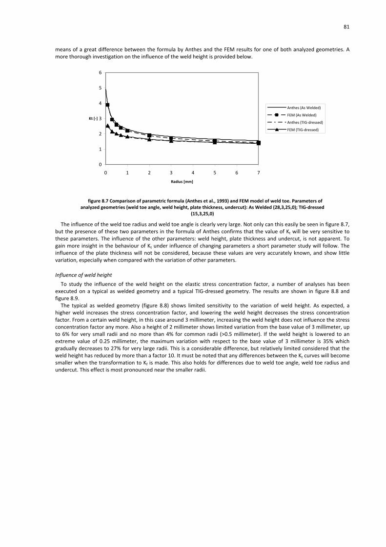
81
means of a great difference between the formula by Anthes and the FEM results for one of both analyzed geometries. A more thorough investigation on the influence of the weld height is provided below.
0
1
2
3
4
5
6
0 1 2 3 4 5 6 7
Radius [mm]
Kt [‐]
Anthes (As Welded)
FEM (As Welded)
Anthes (TIG‐dressed)
FEM (TIG‐dressed)
figure 8.7 Comparison of parametric formula (Anthes et al., 1993) and FEM model of weld toe. Parameters of analyzed geometries (weld toe angle, weld height, plate thickness, undercut): As Welded (28,3,25,0); TIG‐dressed
(15,3,25,0)
The influence of the weld toe radius and weld toe angle is clearly very large. Not only can this easily be seen in figure 8.7, but the presence of these two parameters in the formula of Anthes confirms that the value of Kt will be very sensitive to these parameters. The influence of the other parameters: weld height, plate thickness and undercut, is not apparent. To gain more insight in the behaviour of Kt under influence of changing parameters a short parameter study will follow. The influence of the plate thickness will not be considered, because these values are very accurately known, and show little variation, especially when compared with the variation of other parameters.
Influence of weld height
To study the influence of the weld height on the elastic stress concentration factor, a number of analyses has been executed on a typical as welded geometry and a typical TIG‐dressed geometry. The results are shown in figure 8.8 and figure 8.9. The typical as welded geometry (figure 8.8) shows limited sensitivity to the variation of weld height. As expected, a
higher weld increases the stress concentration factor, and lowering the weld height decreases the stress concentration factor. From a certain weld height, in this case around 3 millimeter, increasing the weld height does not influence the stress concentration factor any more. Also a height of 2 millimeter shows limited variation from the base value of 3 millimeter, up to 6% for very small radii and no more than 4% for common radii (>0.5 millimeter). If the weld height is lowered to an extreme value of 0.25 millimeter, the maximum variation with respect to the base value of 3 millimeter is 35% which gradually decreases to 27% for very large radii. This is a considerable difference, but relatively limited considered that the weld height has reduced by more than a factor 10. It must be noted that any differences between the Kt curves will become smaller when the transformation to Kf is made. This also holds for differences due to weld toe angle, weld toe radius and undercut. This effect is most pronounced near the smaller radii.

82
1
2
3
4
0 1 2 3 4 5 6 7 8
Radius [mm]
Kt [‐]
H=4
H=3
H=2
H=1
H=0.5
H=0.25
figure 8.8 Comparison of Kt for different weld heights for a typical as welded geometry. Parameters of analyzed geometries (weld toe angle, weld height, plate thickness, undercut): (28, ?, 25, 0)
The typical TIG‐dressed geometry (figure 8.9) shows similar behaviour as the typical as welded geometry. From a certain weld height, in this case 2 millimeter, further increase of the height hardly influences the stress concentration factor. A height value of 1 millimeter shows relatively small variations to the base value of 3 millimeter of about 5% over the whole considered range of radii. The extreme case of a weld height of 0.25 millimeter leads to a variation of maximum 18% with respect to the base value of 3 millimeter.
1
2
3
4
0 1 2 3 4 5 6 7 8
Radius [mm]
Kt [‐]
H=3
H=2
H=1
H=0.5
H=0.25
figure 8.9 Comparison of Kt for different weld heights for a typical TIG‐dressed geometry. Parameters of analyzed geometries (weld toe angle, weld height, plate thickness, undercut): (15, ?, 25, 0)
Based on the parameter study it can be concluded that the stress concentration factor is relatively insensitive to weld height variations around commonly observed values. Because all weld heights are recorded they can relatively easily be incorporated in the model, but this conclusion is of great value when the model will be compared to reality later on. When weld heights as low as the weld plateau in typical TIG‐dressed geometry number 3 (see figure 6.9) are considered, a significant influence is observed. This will be addressed later on. It must be noted that this insensitivity of the model to weld height also explains why the model and Anthes’ formula
comply so well for varying weld toe angle while the weld height in the model did not change.
Influence of undercut
To study the influence of the undercut on the elastic stress concentration factor, a number of analyses has been executed on a typical as welded geometry and a typical TIG‐dressed geometry, the results are shown in figure 8.10 and figure 8.11. The stress concentration of the typical as welded geometry (see figure 8.10) increases as expected when an undercut
arises, and increases further when the depth of this undercut increases. For all common measured undercuts (<0.06 millimeter) this variation with respect to the base value of no undercut is not larger than 20%. For common radii (>0.5 millimeter) the variation decreases to 10% or less.

83
1
2
3
4
5
0 1 2 3 4 5 6 7 8
Radius [mm]
Kt [‐]
UC=0
UC=0,1
UC=0,02
UC=0,04
UC=0,06
figure 8.10 Comparison of Kt for different weld heights for a typical as welded geometry. Parameters of analyzed geometries (weld toe angle, weld height, plate thickness, undercut): (28, 3, 25, ?)
The typical TIG‐dressed geometry (see figure 8.11) shows similar behaviour to the as welded geometry, but is a bit more sensitive. For common undercuts the variation has a maximum value of 27%, which decreases to 12% or less when only common radii are considered.
1
2
3
4
0 1 2 3 4 5 6 7 8
Radius [mm]
Kt [-]
UC=0
UC=0,02
UC=0,04
UC=0,06
UC=0,1
figure 8.11 Comparison of Kt for different weld heights for a typical TIG‐dressed geometry. Parameters of analyzed geometries (weld toe angle, weld height ,plate thickness, undercut): (15, 3, 25, ?)
Based on this analysis it can be concluded that the influence of the undercuts that were measured is relatively limited but has to be taken into account in the analysis, with the possible exception of typical TIG‐dressed geometry type 2 (see figure 6.9) where the influence may be larger. While the influence may be limited, the undercut data is available and easily translated into the parametric model. Any influences of the undercut will therefore be taken into account in the fatigue strength prediction. The larger undercuts, such as are present in typical TIG‐dressed geometry type 2, are not present in this analysis.
However, based on the behaviour for smaller undercuts it is very likely that the increase of Kt due to the larger undercut will very probably be smaller than the decrease of Kt due to the very large radius (>10 millimeter) which is commonly associated with this geometry.
Relation between model and reality
The model is of course a simplification of reality. In figure 8.12 a rough overlay of a possible weld geometry and its accompanying model is shown. In two areas the model shows a clear difference with reality. First in the transition from base material into the undercut (marked with line 1 in the figure). Secondly in the transition from the inclined weld material to the top of the weld material (marked with line 2 in the figure). The first difference is rather small, and does not lie in the area of the largest stress concentration. The second difference can be very large. However, the previous parameter study

84
has shown a relative insensitivity of the model to the weld height. The difference of between the two lines in figure 8.12 will therefore not have a large impact on the stress concentration factor at the weld toe. Furthermore, the top of the real weld profile consist of a number of side by side weld beads, and therefore is not completely flat (e.g. see figure 6.3). With the same reasoning as stated above, it can be argued that this will also not influence the stress concentration factor significantly.
weld toe radius
undercut
weld toe angle
weld height
schematisation of weld toe
example of measured weld profile
1 2
figure 8.12 Overlay of an exaggerated possible real weld geometry and the model used to represent this geometry
The possible weld geometry as shown in figure 8.12 can represent most measured geometries, except typical TIG‐dressed type 3 (see figure 6.9). In this weld shape a clear plateau is visible after the weld toe radius. This can be modeled with the available model in two ways. The plateau can be ignored, resulting in too much weld material, or the plateau could be seen as the maximum height of the weld which results in ignoring most of the weld material. The two proposed models and a fictive ‘real’ weld are depicted in figure 8.13.
figure 8.13 Two possible representations of typical TIG‐dressed type 3 and a fictive real weld profile (exaggerated drawings of the weld)
To analyze the consequences of choosing for one of those two models, one typical TIG‐dressed geometry has been modeled to calculate how the stress concentration factor of this geometry will relate to the stress concentration factors of both proposed models. The results are presented in figure 8.14. It is clear that the ‘real’ model lies in between the two proposed models. Because of time constraints, in this research the choice will be made for one of both models. This will be the model on the right in figure 8.14 because here the difference with the ‘real’ model is the smallest. It must be noted that this approximation only has to be made for the specific geometries which show a plateau in the weld.
figure 8.14 Outcome of three different models for the same weld (exaggerated drawings of the weld)
8.3.2 Determination of Kt Fatigue is a weakest link process. This property makes it very hard to predict the combination of geometry parameters
which have to be taken into account to create the ‘characteristic weld toe’ in a model. The fact that the TIG‐dressed weld toe radii showed significant spread and a small additional peak near the main peak of the as welded radii, indicating a possible lack of improvement of this ‘characteristic weld toe’, makes the analysis even more complicated. The choice is made to execute two types of analyses, one where for all parameters the main peak value is considered
both for as welded and TIG‐dressed specimens and one where the radius of the TIG‐dressed specimens has a similar value as the as welded radii while all other parameters are assumed to be at their peak value. Subsequently, influencing parameters will be varied, resulting in an expected bandwidth of Kt.

85
Some parameters will be calculated, such as the mean of the, nearly normal distributed, weld toe angles. Others will be estimated with the aid of the diagrams provided in 6.3.4. This introduces some extra uncertainty, but calculation would require the fitting of a probability density function, which also has an error margin, especially when the results do not fit the distribution very well. If the results of the laser measurements of the weld toe would have been categorized and any possible dependencies would have been documented, a statistic analysis could be performed which can, based on the occurrence of different geometries, more accurately predict the mean and standard deviation of Kt. Because such elaborate documentation of the weld toe parameters has been omitted in this research, the variation of Kt and Kf will be based on estimates.
First analysis, peak values
The base values of this analysis are depicted in table 8.2. It is indicated in the table for each variable how it has been determined.
As welded TIG‐dressed determined by
Weld toe radius [mm] 1.0 3.8 estimate
Weld toe angle [‐] 27.8 15.3 calculated mean
Weld height [mm] C11 3.9 3.9 calculated mean
C89 4.1 4.1 calculated mean
C89a 4.3 4.3 calculated mean
C69 2.3 2.3 calculated mean
C46 1.8 1.8 calculated mean
V11 3.7 3.7 calculated mean
V89 3.0 3.0 calculated mean
V69 2.5 2.5 calculated mean
V46 2.1 2.1 calculated mean
Undercut [mm] 0 0 estimate
Plate thickness [mm] S1100 20 20 measured
other 25 25 measured
table 8.2 Peak values of weld toes
The weld toe as described in table 8.2 will be considered as the base value. A short sensitivity analysis will follow, where all values are related to this base value. In figure 8.15 to figure 8.18 the results are presented for a variation of a certain amount to both sides of the chosen base value. The diagram shows the variation of Kt in relation to its base value as stated in table 8.2, when this base value is varied (see also equation (8.4)). For the weld toe angle and radius the values are varied for one standard deviation to both sides of the base value. For the undercut a value of 0.06 was chosen, based on the diagrams in 6.3.4. The weld height is varied over a wider band to cover the mean and standard deviation of all considered plates and has a base value (valued 1 in the graph) of 3. The assumption is that the influence of one parameter is not influenced by the change of another parameter. If for example the radius is determined at a slightly different value, it is assumed that the influence of the weld toe angle (see figure 8.16) is similar. Based on observations on the diagrams below, this seems a reasonable assumption because the diagrams all look similar while they are determined for two very different geometries.
0.85
0.9
0.95
1
1.05
1 1.5 2 2.5 3 3.5 4 4.5 5
Weld height [mm]
fwh
[‐]
0.85
0.9
0.95
1
1.05
1 1.5 2 2.5 3 3.5 4 4.5 5
Weld height [mm]
fwh
[‐]
t=25
t=20
figure 8.15 Variation of Kt with variating weld height for as welded (left) and TIG‐dressed joints (right)
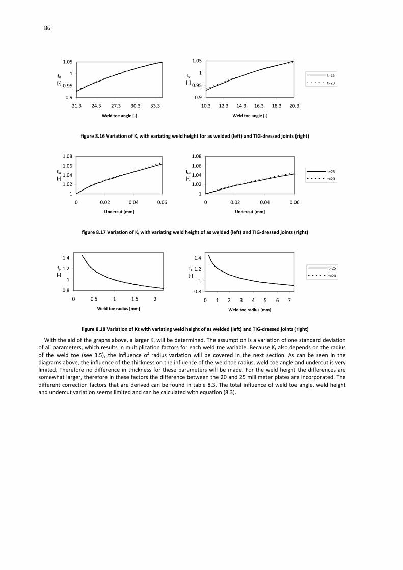
86
0.9
0.95
1
1.05
21.3 24.3 27.3 30.3 33.3
Weld toe angle [‐]
fΘ
[‐]
0.9
0.95
1
1.05
10.3 12.3 14.3 16.3 18.3 20.3
Weld toe angle [‐]
fΘ
[‐]
t=25
t=20
figure 8.16 Variation of Kt with variating weld height for as welded (left) and TIG‐dressed joints (right)
1
1.02
1.04
1.06
1.08
0 0.02 0.04 0.06
Undercut [mm]
fuc
[‐]
1
1.02
1.04
1.06
1.08
0 0.02 0.04 0.06
Undercut [mm]
fuc
[‐]
t=25
t=20
figure 8.17 Variation of Kt with variating weld height of as welded (left) and TIG‐dressed joints (right)
0.8
1
1.2
1.4
0 0.5 1 1.5 2
Weld toe radius [mm]
fρ
[‐]
0.8
1
1.2
1.4
0 1 2 3 4 5 6 7
Weld toe radius [mm]
fρ
[‐]
t=25
t=20
figure 8.18 Variation of Kt with variating weld height of as welded (left) and TIG‐dressed joints (right)
With the aid of the graphs above, a larger Kt will be determined. The assumption is a variation of one standard deviation of all parameters, which results in multiplication factors for each weld toe variable. Because Kf also depends on the radius of the weld toe (see 3.5), the influence of radius variation will be covered in the next section. As can be seen in the diagrams above, the influence of the thickness on the influence of the weld toe radius, weld toe angle and undercut is very limited. Therefore no difference in thickness for these parameters will be made. For the weld height the differences are somewhat larger, therefore in these factors the difference between the 20 and 25 millimeter plates are incorporated. The different correction factors that are derived can be found in table 8.3. The total influence of weld toe angle, weld height and undercut variation seems limited and can be calculated with equation (8.3).

87
As welded TIG‐dressed
Base value Varied to Factor fi Base value Varied to Factor fi
Weld toe angle [‐] 27.8 34.4 1.05 15.3 20.2 1.05
Weld height [mm] C11 3.9 4.4 1 3.9 4.4 1
C89 4.1 4.4 1 4.1 4.4 1
C89a 4.3 4.5 1 4.3 4.5 1
C69 2.3 2.5 1.01 2.3 2.5 1
C46 1.8 2.0 1.01 1.8 2.0 1
V11 3.7 3.9 1 3.7 3.9 1
V89 3.0 3.3 1.01 3 3.3 1
V69 2.5 2.6 1 2.5 2.6 1
V46 2.1 2.3 1.01 2.1 2.3 1
Undercut [mm] 0 0.03 1.04 0 0.05 1.04
table 8.3 Influence factors for variation of one standard deviation of weld toe angle, weld height and undercut
;t adj uc whK f f f (8.3)
In which: fΘ= influence factor for variation of weld toe angle [‐] fuc= influence factor for variation of undercut [‐] fwh= influence factor for weld height [‐]
t
i
t
K i base valuef
K i base value
(8.4)
Second analysis, no improvement in TIG‐dressed radius
For this analysis all values of the as welded weld toe are the same as stated in table 8.2. The values of the TIG‐dressed specimen are also assumed the same, with the exception of the weld toe radius. Based on observations on figure 6.22 it is very well possible that the weakest link radius of the TIG‐dressed specimens has a similar value as in the as welded specimen, resulting in a base value radius of 1 millimeter. An additional sensitivity for the new TIG‐dressed base geometry is presented in figure 8.19 and figure 8.20.
0.85
0.9
0.95
1
1.05
1 1.5 2 2.5 3 3.5 4 4.5 5
Weld height [mm]
fwh
[-]
0.85
0.95
1.05
10.3 12.3 14.3 16.3 18.3 20.3
Weld toe angle [‐]
fΘ
[‐]
t=25
t=20
figure 8.19 Variation of Kt with variating weld height (left) and weld toe angle (right) for the TIG‐dressed weld toe
1
1.02
1.04
1.06
1.08
1.1
0 0.02 0.04 0.06
Undercut [mm]
fuc
[‐]
0.75
1
1.25
1.5
0 1 2 3 4 5 6 7
Weld toe radius [mm]
fρ
[‐]
t=25
t=20
figure 8.20 Variation of Kt with variating undercut (left) and weld toe radius (right) for the TIG‐dressed weld toe
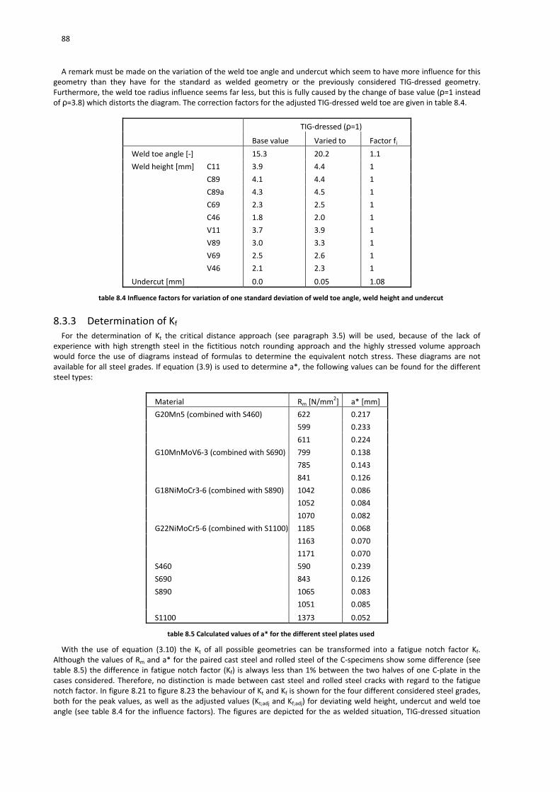
88
A remark must be made on the variation of the weld toe angle and undercut which seem to have more influence for this geometry than they have for the standard as welded geometry or the previously considered TIG‐dressed geometry. Furthermore, the weld toe radius influence seems far less, but this is fully caused by the change of base value (ρ=1 instead of ρ=3.8) which distorts the diagram. The correction factors for the adjusted TIG‐dressed weld toe are given in table 8.4.
TIG‐dressed (ρ=1)
Base value Varied to Factor fi
Weld toe angle [‐] 15.3 20.2 1.1
Weld height [mm] C11 3.9 4.4 1
C89 4.1 4.4 1
C89a 4.3 4.5 1
C69 2.3 2.5 1
C46 1.8 2.0 1
V11 3.7 3.9 1
V89 3.0 3.3 1
V69 2.5 2.6 1
V46 2.1 2.3 1
Undercut [mm] 0.0 0.05 1.08
table 8.4 Influence factors for variation of one standard deviation of weld toe angle, weld height and undercut
8.3.3 Determination of Kf For the determination of Kt the critical distance approach (see paragraph 3.5) will be used, because of the lack of
experience with high strength steel in the fictitious notch rounding approach and the highly stressed volume approach would force the use of diagrams instead of formulas to determine the equivalent notch stress. These diagrams are not available for all steel grades. If equation (3.9) is used to determine a*, the following values can be found for the different steel types:
Material Rm [N/mm2] a* [mm]
G20Mn5 (combined with S460) 622 0.217
599 0.233
611 0.224
G10MnMoV6‐3 (combined with S690) 799 0.138
785 0.143
841 0.126
G18NiMoCr3‐6 (combined with S890) 1042 0.086
1052 0.084
1070 0.082
G22NiMoCr5‐6 (combined with S1100) 1185 0.068
1163 0.070
1171 0.070
S460 590 0.239
S690 843 0.126
S890 1065 0.083
1051 0.085
S1100 1373 0.052
table 8.5 Calculated values of a* for the different steel plates used
With the use of equation (3.10) the Kt of all possible geometries can be transformed into a fatigue notch factor Kf. Although the values of Rm and a* for the paired cast steel and rolled steel of the C‐specimens show some difference (see table 8.5) the difference in fatigue notch factor (Kf) is always less than 1% between the two halves of one C‐plate in the cases considered. Therefore, no distinction is made between cast steel and rolled steel cracks with regard to the fatigue notch factor. In figure 8.21 to figure 8.23 the behaviour of Kt and Kf is shown for the four different considered steel grades, both for the peak values, as well as the adjusted values (Kt;adj and Kf;adj) for deviating weld height, undercut and weld toe angle (see table 8.4 for the influence factors). The figures are depicted for the as welded situation, TIG‐dressed situation
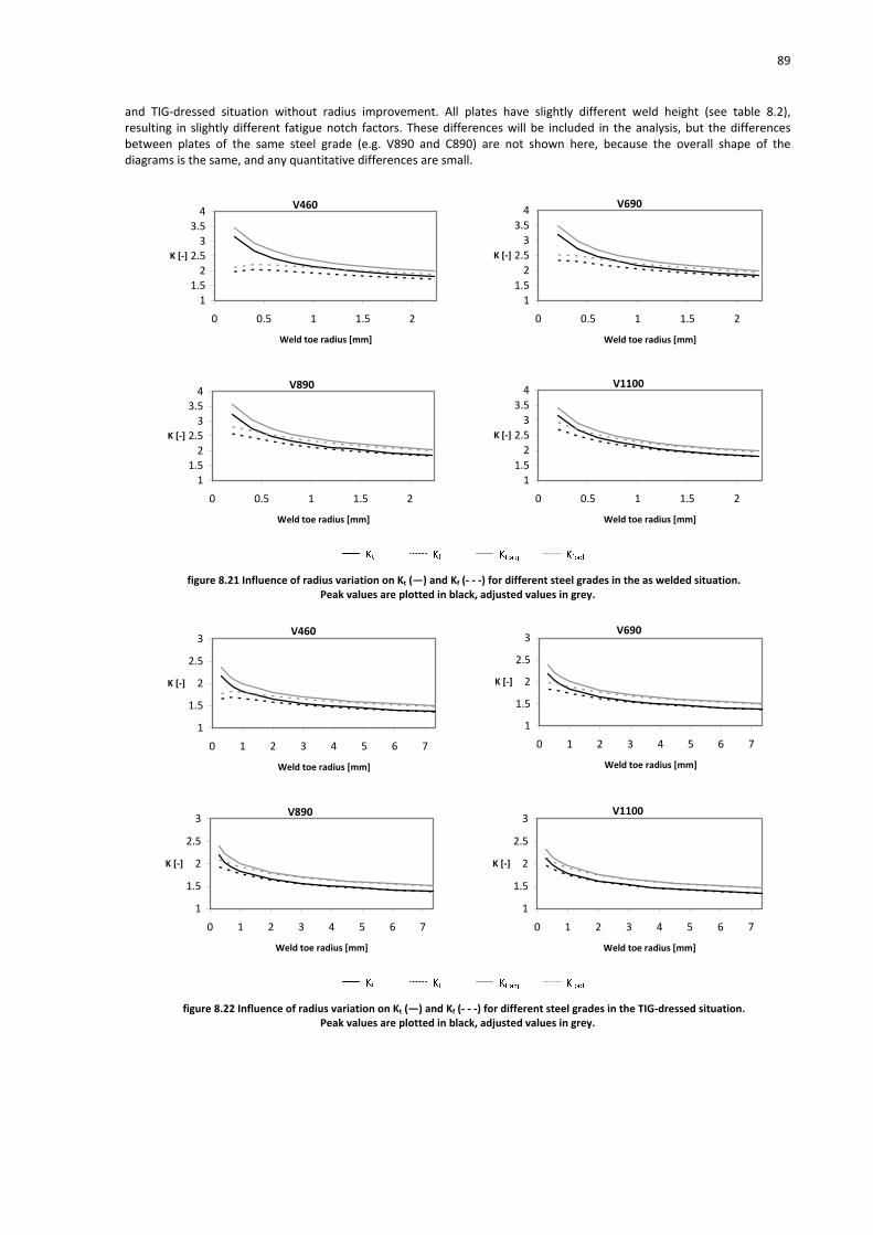
89
and TIG‐dressed situation without radius improvement. All plates have slightly different weld height (see table 8.2), resulting in slightly different fatigue notch factors. These differences will be included in the analysis, but the differences between plates of the same steel grade (e.g. V890 and C890) are not shown here, because the overall shape of the diagrams is the same, and any quantitative differences are small.
V460
1
1.5
2
2.5
3
3.5
4
0 0.5 1 1.5 2
Weld toe radius [mm]
K [‐]
V690
1
1.5
2
2.5
3
3.5
4
0 0.5 1 1.5 2
Weld toe radius [mm]
K [‐]
V890
1
1.5
2
2.5
3
3.5
4
0 0.5 1 1.5 2
Weld toe radius [mm]
K [‐]
V1100
1
1.5
2
2.5
3
3.5
4
0 0.5 1 1.5 2
Weld toe radius [mm]
K [‐]
figure 8.21 Influence of radius variation on Kt (―) and Kf (‐ ‐ ‐) for different steel grades in the as welded situation. Peak values are plotted in black, adjusted values in grey.
V460
1
1.5
2
2.5
3
0 1 2 3 4 5 6 7
Weld toe radius [mm]
K [‐]
V690
1
1.5
2
2.5
3
0 1 2 3 4 5 6 7
Weld toe radius [mm]
K [‐]
V890
1
1.5
2
2.5
3
0 1 2 3 4 5 6 7
Weld toe radius [mm]
K [‐]
V1100
1
1.5
2
2.5
3
0 1 2 3 4 5 6 7
Weld toe radius [mm]
K [‐]
figure 8.22 Influence of radius variation on Kt (―) and Kf (‐ ‐ ‐) for different steel grades in the TIG‐dressed situation. Peak values are plotted in black, adjusted values in grey.

90
V460
1
1.5
2
2.5
3
0 1 2 3 4 5 6 7
Weld toe radius [mm]
K [‐]
V690
1
1.5
2
2.5
3
0 1 2 3 4 5 6 7
Weld toe radius [mm]
K [‐]
V890
1
1.5
2
2.5
3
0 1 2 3 4 5 6 7
Weld toe radius [mm]
K [‐]
V1100
1
1.5
2
2.5
3
0 1 2 3 4 5 6 7
Weld toe radius [mm]
K [‐]
figure 8.23 Influence of radius variation on Kt (―) and Kf (‐ ‐ ‐) for different steel grades in the TIG‐dressed situation without radius improvement. Peak values are plotted in black, adjusted values in grey.
The fatigue strength curve of each material will be determined for different cases. One analysis uses the peak value of the weld toe radius, combined with the peak value of all other weld toe parameters. In case of the TIG‐dressed situation without radius improvement an exception is made for the weld toe radius, which is kept at the peak value of the as welded situation. Another analysis will be made using the weld toe parameters which are corrected to simulate the possibility of a ‘weakest link’. All parameters except the weld toe radius were already varied over a value of one standard deviation in 8.3.2. A similar variation of the weld toe radius would lead to very small differences between the three considered situations, because especially the TIG‐dressed radii show a large standard deviation. Because small radii in combination with other TIG‐dressed weld toe parameters are already covered in a separate situation, such a large variation is deemed too conservative and is therefore omitted. The chosen variation of the weld toe radius is determined at half of its peak value, which covers the bulk of the weld toe radii (see 6.3.4). This leads to an adjusted weld toe radius of 0.5 millimeter for the as welded situation and an adjusted weld toe radius of 1.9 millimeter for the TIG‐dressed situation. The calculated stress concentration factors and fatigue notch factors for both the peak values (Kt and Kf) and the corrected values after variation of the weld toe parameters (Kt;adj and Kf;adj) can be found in table 8.6 and table 8.7. Some slight differences may exist between the cast and rolled side of the specimens. This is not depicted in table 8.6 and table 8.7, but is incorporated in the model and the comparison with the fatigue tests in 9.4.3.
As welded TIG‐dressed TIG‐dressed (ρ=1)
Kt Kt;adj Kt Kt;adj Kt Kt;adj
C1100 2.16 2.79 1.47 1.78 1.79 2.35
C890 2.26 2.92 1.52 1.84 1.85 2.43
C890a 2.26 2.92 1.52 1.84 1.85 2.42
C690 2.17 2.83 1.50 1.82 1.83 2.40
C460 2.11 2.75 1.49 1.81 1.81 2.38
V1100 2.15 2.78 1.47 1.78 1.79 2.35
V890 2.22 2.89 1.52 1.84 1.84 2.42
V690 2.19 2.82 1.51 1.83 1.83 2.41
V460 2.15 2.80 1.50 1.82 1.82 2.39
table 8.6 Calculated elastic stress concentration factors for the three distinguished situations for peak values and adjusted values

91
As welded TIG‐dressed TIG‐dressed (ρ=1)
Kf Kf;adj Kf Kf;adj Kf Kf;adj
C1100 2.10 2.61 1.47 1.76 1.75 2.22
C890 2.16 2.63 1.51 1.80 1.78 2.22
C890a 2.16 2.64 1.51 1.80 1.78 2.22
C690 2.04 2.45 1.49 1.77 1.74 2.12
C460 1.91 2.19 1.46 1.72 1.66 1.95
V1100 2.10 2.61 1.47 1.76 1.75 2.22
V890 2.12 2.61 1.50 1.80 1.77 2.21
V690 2.05 2.44 1.49 1.77 1.74 2.12
V460 1.93 2.20 1.47 1.72 1.66 1.94
table 8.7 Calculated fatigue notch factors for the three distinguished situations for peak values and adjusted values
8.4 Determination of mean stress factor The fatigue strength of specimens is also influenced by a mean stress (see figure 2.7). This mean stress is determined by
the stress ratio R (see 2.3.2) and by the residual stress σr. For welded connections, a residual stress equal in magnitude to the yield stress is usually assumed. The TIG‐dressing process is expected to lower residual stresses. Due to time limitations, measurements on residual stresses could not be done. To make a reasonable assumption, reference is made to literature. As shown in 4.3.3, Lopez Martinez has investigated the residual stress before and after TIG dressing. Before TIG‐dressing he found a residual stress at the surface of 0.61σy, which was reduced to 0.43 σy after TIG‐dressing. In deeper layers of the material the residual stress increased, but because the cracks are assumed to initiate at the surface, which is well supported by observations on the specimens, a similar residual stress reduction is assumed to occur in the specimens. When for the as welded specimens σr= σy is assumed, the residual stress after TIG‐dressing can be assumed as:
0.43
0.70.61
r y y (8.5)
The mean stress of all specimens will be adjusted to a value of σm=½σy. Therefore the analytical values will also be
adjusted to this value. Based on Haibach (2006), Pijpers (2011) proposed equation (8.6) to determine a mean stress factor including the effect of residual stresses:
;0
;0
;0
;
;0
;0
2
;0
1when 1
1
1when 1 1
1
13 when 1 3
1 13
13 when 3
1
m r
f aE
m r
m r aEf
aE
m Haibach
f
m r
aEf m rf
aE
f
m r
aEf
M
M
fM
MM
M
M
(8.6)
with 0.00035 0.1f mM R

92
In which:
fm;Haibach ;0 m
;0 m
for 0 and 0
for 0 and 0aE r
aE r
Mf mean stress subfactor [N/mm2] σm mean stress [N/mm2] σr residual stress [N/mm2] σaE;0 fatigue endurance strength at alternating load [N/mm2]
8.5 Determination of thickness factor The plate thickness of a specimen can influence the fatigue strength. Thicker plates generally show less favourable
fatigue behaviour. The calculation procedure as described in this chapter leads to the fatigue resistance at a reference thickness of 25 millimeter. Because the fatigue test results are all adjusted to a thickness of 25 millimeter, the fatigue strength prediction does not need to be adjusted. The determination and use of the thickness factor will be explained in 9.2.2.
8.6 Determination of loading mode factor The method that is used refers to tensile loading of the specimens. In the fatigue testing in this research also only tensile
loading will be applied. Due to misalignments the load will be partly in bending, but only the results of the actual tests will be adjusted for any influence of the bending loading mode. The fatigue strength prediction will refer to pure tension, thus eliminating the need for any loading mode factor. The correction of the fatigue test results will be explained in 9.2.2.
8.7 Prediction of fatigue strength curve The fatigue strength curve for crack initiation is determined in several steps. First the fatigue limit of the base material is
determined with equation (8.1). This value is then corrected for notches, mean and residual stress and displayed as a stress range instead of a stress amplitude, see equation (8.7).
; ; ;0
2E specimen m a E
f
fK
(8.7)
Subsequently, the fatigue strength curve is determined with either the approach by Schijve or Hück et al. (see 3.5.1). The
knee point for the fatigue strength curve in the approach by Schijve is set at 2∙107 according to the recommendation in his publication (see 3.5.1). This results in several design lines per plate. First of all there are the three considered situations: as welded, TIG‐dressed,
and TIG‐dressed without radius improvement. Furthermore, to investigate the sensitivity of the fatigue strength to variation of the weld toe parameters, two values for Kf have been calculated in 8.3.2 and 8.3.3. One of these values, Kf;adj is the result of an unfavourable variation of all weld toe parameters for a certain amount. This variation does not result in a specific failure chance, and has no more value than a sensitivity analysis. The difference between the lines determined with Kf and Kf;adj gives insight in the sensitivity of the results for slight variation of the weld toe geometry. This will be commented on in 9.4.3.

93
9 Analysis of fatigue test results
9.1 Chapter outline In this chapter the fatigue data will be analyzed. First, a selection and adjustment of the test data will be discussed. Then
the statistical analysis of the data follows, which leads to mean and characteristic S‐N curves. In paragraph 9.3, the data of the TIG‐dressed specimens is compared with different design codes, as welded data and the analytical determination of the fatigue strength. The influence of TIG‐dressing is summarized in paragraph 9.4.
9.2 Analysis of raw data
9.2.1 Exclusion of data Not al data is deemed representative for analysis. In some cases the failure mechanism that was observed cannot occur
in common practice. These data points will therefore be excluded and not be used in the statistical analysis of the fatigue data, but can still be found in the tabulated fatigue results in Annex C.
Excluded data
The data points of the following specimens have been excluded from analysis:
C46‐2
C69‐3
C89‐2
V11‐1 Due to a failure of the testing rig, specimen C46‐2 has been compressed and has buckled (see figure 9.1). The permanent
deformation resulting from this buckling or the straightening needed for testing will very probably influence the result, if the specimens is tested for fatigue strength. Therefore specimen C46‐2 was not tested, and is thus absent in the fatigue data tabulation in Annex C.
figure 9.1 Damaged specimen C46‐2
The backside of plate C69 could not be TIG‐dressed (see 5.2.2). This resulted in a weld root with rather sharp notches (see figure 9.2). With specimen C69‐1 this still resulted in weld cap failure, but at specimen C69‐3 these notches initiated a crack on the back of the specimen. Because notches of these depth and sharpness will never pass quality control in any practical structure, this data point is eliminated. To prevent a similar failure with specimen C69‐2, the weld root was ground smooth.

94
figure 9.2 Backside of specimen C69‐1 with sharp notches at the weld root
C82‐2 showed very large flaws in the cast plate, with depths of a few millimeters. To repair the plate these flaws were removed by milling and the resulting grooves were filled with weld material. Unfortunately, also the repaired specimen was not free of flaws in the cast base plate. Furthermore, the weld root could not be TIG‐dressed (see also 5.2.2). This resulted in simultaneous crack initiation in the parent material and the weld root. Because both crack initiation sites would not have passed quality control in practice, this data point is eliminated. In figure 7.6 it can clearly be seen that one data point does not cohere with the rest of the data. This specimen (V11‐1)
has failed in the parent material, on the root side of the weld. On the root side of the weld, stresses are much lower due to the misalignment. Although no clear defect could be found which can lead to exclusion of this data point, the data point will not be included in the analysis. It is reasonable to assume that the defect that caused the initiation of this crack has not been influenced by the TIG dressing because the crack occurred at the relatively large distance of a few centimeters from the weld toe. If this specimen had not been TIG‐dressed, the crack would likely arise at the same location, because the data point also lies lower than most as welded data points which were tested by Pijpers (2011). Therefore, for the investigation of the influence of TIG‐dressing, this specimen provides no useful information.
Reruns of specimens
Some specimens have shown crack initiation in the base material. Three of those base material cracks were outside of the cross section reduction. This concerns the specimens:
C11‐2
C89‐1
C89‐2 As described above, C89‐2 will be excluded from the analysis. The remaining two specimens have a clear crack initiation
site at a flaw in the material, which could have been visually assessed during quality control. Because the crack occurred at a significant distance from the cross section reduction it was possible to continue testing the specimen after it failed in the base material at approximately the same stress level. For several reasons the stress level of a second test will never be at exactly the same level. This is caused by the reduced specimen length, resulting in a changed misalignment, and the uncertainty where cracks will initiate. The stresses in the second test are matched to stresses in the first test from a strain gauge close to a likely, highly stressed, crack initiation point. This is not necessarily the crack initiation point of the second test. To calculate the combined stress for the final result, equation (9.1) has been used.
1 21 2
1, , , , ,
; ;
1m mm m
i i S d L d j j S dm
eq S d
i j
n n
D n n
(Hobbacher, 2007) (9.1)
In which: D Miner sum of total damage [‐] Δσi,S,d value of characteristic equivalent stress range [N/mm2] m1 slope of S‐N curve above the knee point [‐] m2 slope of S‐N curve below the knee point [‐] Δσi,S,d stress ranges (loads) above the knee point [N/mm2] Δσj,S,d stress ranges (loads) below the knee point [N/mm2] ΔσL,d stress range (resistance) at the knee point of the S‐N curve [N/mm2] ni number of cycles belonging to Δσi [‐] nj number of cycles belonging to Δσj [‐] In the calculation the Miner sum of total damage is assumed to be 1. All stress ranges are assumed to lie above the knee
point of the S‐N curve, thereby omitting the need for values of m2 and ΔσL,d. The slope of the S‐N curve above the knee

95
point (m1) is assumed to be 3. All these assumptions do not influence the result much because the stress ranges of the two tests are relatively close together. Other equivalent parameters are combined according to the number of cycles of each test, see equation (9.2). The limited influence of the assumptions for equation (9.1) show when equation (9.2) is used for the calculation of the combined stress: practically the same combined stress follows from both formulas.
I I II IIeq
I II
X n X nX
n n
(9.2)
In which: Xeq equivalent parameter [‐] XI parameter value in first test [‐] NI number of cycles in first test [‐] XII parameter value in second test [‐] nII number of cycles in second test [‐] All presented results in graphs for specimen C11‐2 and C89‐1 represent the results of the final failure. In the tabulated
test results in Annex C the values from the separated tests are available together with their combined value.
Failure outside weld region
Finally, some specimens must be mentioned which have shown failure outside the weld region, but will not be excluded from the data:
C11‐1
C11‐2 (after rerun)
V11‐1
C89‐1 (after rerun) All specimens show a crack in the parent material, but inside the reduced cross section. Because there is no clear, large
defect at which the crack has initiated which should not pass quality control in practice, these data points will not be excluded from the analysis. Their failure mode however, is different from all weld toe or weld material cracks. This could either be the result of a defect and the higher sensitivity of very high strength steels (especially S1100) for these defects (see 4.2.2) or an improvement of the fatigue strength in the weld region, caused by TIG‐dressing. Such an improvement may have led to the base material being the weakest link. These data points will be marked in graphs to identify them if they show significant different behaviour than the other specimens. Any base material failures from the as welded tests will also be marked. If the base material failures after TIG‐dressing show better fatigue behaviour than the as welded base material failures, this may be an indication that the base material failures in this research may have been caused by improving the weld toe, and shifting the weakest link to the base material. Failures in the weld material are considered to necessarily be an improvement of the connection, because such failures did not occur in the research by Pijpers. For this reason these results are judged as regular and will not be marked separately. In Annex C all different failure mechanisms are listed per specimen.
9.2.2 Adjustment of test data To correctly compare the test data to the standardized cases in design codes, and to the previous experiments carried
out by Pijpers (2011), the nominal stress levels will be adjusted. For the definition and determination of these factors this research relies to a great extent on the work by Pijpers (2011). Correction factors will be applied to correct for:
Mean stress; nominal stresses are adjusted to a mean stress value of σm=0.5∙σy
Residual stress; nominal stresses are adjusted to a loading with a certain representative residual stress
Thickness; nominal stresses are adjusted to a reference thickness of 25 millimeter
Loading mode; nominal stresses are adjusted to a pure tension loading mode The adjusted nominal stress can then be calculated with the use of equation (9.3) for base material cracks and equation
(9.4) for weld toe cracks.
; ;
; ; ; ;
1 1
f f
n u Nf m n
t u N lm u N
ff f
(9.3)
In which: fm Mean stress factor [‐] ft;u;Nf Thickness factor for fatigue life of base material cracks [‐] flm;u;Nf Loading mode factor for fatigue life of base material cracks [‐]
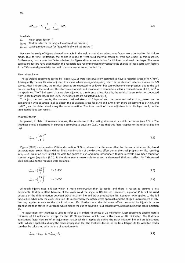
96
; ;
; ; ; ;
1 1
f f
n w Nf m n
t w N lm w N
ff f
(9.4)
In which: fm Mean stress factor [‐] ft;w;Nf Thickness factor for fatigue life of weld toe cracks [‐] flm;w;Nf Loading mode factor for fatigue life of weld toe cracks [‐] Because the study of Pijpers showed no cracks in the weld material, no adjustment factors were derived for this failure
mode. Due to time limitations, the choice is made to treat weld material cracks as weld toe cracks in this research. Furthermore, most correction factors derived by Pijpers show some variation for thickness and weld toe shape. The same corrections factors have been used in this research. It is recommended to investigate the change in these correction factors if the TIG‐dressed geometries and weld material cracks are accounted for.
Mean stress factor
The as welded specimens tested by Pijpers (2011) were conservatively assumed to have a residual stress of 0 N/mm2. Subsequently the results were adjusted to a value where σr= σy and σm=½σy, which is the standard reference value for S‐N curves. After TIG‐dressing, the residual stresses are expected to be lower, but cannot become compressive, due to the still present cooling of the weld toe. Therefore, a reasonable and conservative assumption still is a residual stress of 0 N/mm2 in the specimen. The TIG‐dressed data are also adjusted to a reference value. For this, the residual stress reduction deducted from Lopez Martinez (see 8.4) is used. The test results are adjusted to σr=0.7σy To adjust the test results, the assumed residual stress of 0 N/mm2 and the measured value of σm were used in
combination with equation (8.6) to obtain the equivalent stress for σm=0 and σr=0. From there adjustment to σm=½σy and σr=0.7σy can be determined using the same equation. The total result of these adjustments is displayed as fm in the tabulated fatigue test results.
Thickness factor
In general, if plate thicknesses increase, the resistance to fluctuating stresses at a notch decreases (see 2.3.1). The thickness effect is described in Eurocode according to equation (9.5). Note that this factor applies to the total fatigue life (Nf)
0.2
; ;
25ft w Nf
t
(9.5)
Pijpers (2011) used equation (9.6) and equation (9.7) to calculate the thickness effect for the crack initiation life, based
on a parameter study. Pijpers did not find a confirmation of the thickness effect during the crack propagation life, resulting in ft;w;Np=1. Equation (9.6) is valid for weld toe angles of 25°, and more pronounced thickness effects have been found for steeper angles (equation (9.7)). It therefore seems reasonable to expect a decreased thickness effect for TIG‐dressed specimens due to the reduced weld toe angle.
0.4
; ;
25it w Nf
t
for Θ=25° (9.6)
0.7
; ;
25it w Nf
t
for Θ=65° (9.7)
Although Pijpers uses a factor which is more conservative than Eurocode, and there is reason to assume a less
detrimental thickness effect because of the lower weld toe angle in TIG‐dressed specimens, equation (9.6) will be used because of the differentiation between crack initiation life and crack propagation life. Equation (9.5) applies to the full fatigue life, while only the crack initiation life is covered by the notch stress approach and the alleged improvement of TIG‐dressing applies mainly to the crack initiation life. Furthermore, the thickness effect proposed by Pijpers is more pronounced than stated in Eurocode which makes the use of equation (9.6) conservative, at least during the crack initiation life. The adjustment for thickness is used to refer to a standard thickness of 25 millimeter. Most specimens approximate a
thickness of 25 millimeter, except for the S1100 specimens, which have a thickness of 20 millimeter. The thickness adjustment factor consists of an adjustment factor which is applicable during the crack initiation life and an adjustment factor which is applicable during the crack propagation life. The thickness factor for the total fatigue life for weld toe cracks can then be calculated with the use of equation (9.8).
; ; ; ; ; ;f i i p pt w N t w N N t w N Nf f f f f (9.8)

97
In which: ft;w;Ni Thickness factor for crack initiation life [‐] fNi Crack initiation life ratio [‐] ft;w;Np Thickness factor for crack propagation life [‐] fNp Crack propagation life ratio [‐] Pijpers did not find a thickness effect for base material cracks, resulting in ft;u;Nf=ft;u;Ni=ft;u;Np=1.
Loading mode factor
The adjustment for loading mode is used to refer to a standard loading mode of pure tension. Because all specimens had a certain misalignment, part of the load was bending. The correction factor can be calculated with the use of equation (9.9) for base material cracks and equation (9.10) for weld toe cracks.
; ; ; ; ; ;f i i p plm u N lm u N N lm u N Nf f f f f (9.9)
In which: flm;u;Ni Loading mode factor for crack initiation life; 1.0 (Pijpers, 2011) [‐] fNi Crack initiation life ratio [‐] flm;u;Np Loading mode factor for crack propagation life; 1.09 (Pijpers, 2011) [‐] fNp Crack propagation life ratio [‐]
; ; ; ; ; ;f i i p plm w N lm w N N lm w N Nf f f f f (9.10)
In which: flm;w;Ni Loading mode factor for crack initiation life; 1.2 (Pijpers, 2011) [‐] fNi Crack initiation life ratio [‐] flm;w;Np Loading mode factor for crack propagation life; 1.37 (Pijpers, 2011) [‐] fNp Crack propagation life ratio [‐] The applicable correction factor for the misaligned axially loaded specimens can be calculated with the use of equation
(9.11).
; ; ;
; ;
11
f
mlm w N ax
m
lm w Nf
Kf
K
f
(9.11)
In which: Km Misalignment factor. [‐] Hobbacher (2007) proposed a formula based on geometry to calculate a stress increase
factor. In this research Km is based on the ratio between F/A and the measured stress near the weld [‐] flm;w;Nf Loading mode factor for total fatigue life for weld toe cracks. [‐] If base material cracks are considered, flm;w;Nf is
replaced by flm;u;Nf (cracks in the weld material will regarded as weld toe cracks) [‐]
9.2.3 Statistical analysis The fatigue data are analyzed according to the method described by Brozzetti et al. (1989) which is also prescribed by
Eurocode. For a given dataset a mean regression line is constructed with a survival probability of 50% (see equation (9.12))
i N iy a b x (9.12)
In which: yi Log Nf [‐] xi Log Δσ [‐] aN intersection on log N axis [‐] b regression coefficient [‐] ε sum of unknown random errors [‐] The residual random errors ε are minimized when aN and b are estimated with the least squares method:

98
22
i i i i
i i
n x y x yb
n x x
(9.13)
1N i ia y b x
n (9.14)
In which: n number of specimens [‐] The slope of the S‐N curve (b from equation (9.13)) can either be determined by the least squares method, or fixed to a
certain value. Especially for small batches of fatigue tests (smaller than 10) the fixed value of the slope is a sensible solution. A common value for the slope is 3 for as welded joints. As mentioned in 4.3.4, different authors have found the slope to increase (i.e. a flatter S‐N curve) when TIG‐dressing is applied. Therefore, although the number of specimens is limited, an S‐N curve with a free slope and a fixed slope of ‐3 will both be determined. For comparison with Eurocode detail categories and as welded data, the mean stress range with a probability of survival
of 50% and 95% at N = 2∙106 cycles is calculated. The mean stress with a 50% probability of survival at 2∙106 is calculated with equations (9.15), (9.16) and (9.17).
50%
50% 10x (9.15)
50%50%
Ny ax
b
(9.16)
650% log 2 10y (9.17)
To calculate the stress range with a 95% survival probability, the coefficient of variation first needs to be determined. This
can be done with equation (9.18).
2
2
2
when b is calculated2
when b is fixed1
i N i
i N i
y a b x
ns
y a b x
n
(9.18)
In which: s coefficient of variation [‐] Now the characteristic stress range at 2∙106 cycles is calculated for a 75% confidence level of 95% probability of survival.
As statistical distribution the student‐t‐distribution is used.
95%
95% 10x (9.19)
50% 95%95%
log y ax
b
(9.20)
95% 50% 0.95;n fa a t s (9.21)
In which: t0,95;n‐f The student‐t‐distribution factor for n‐f degrees of freedom and a 95% probability of survival. n is the amount of
data points, f is 1 for a fixed b‐value and 2 for a calculated b value. [‐] Brozetti has stated some conditions for these formulas to give a reliable result. Runouts should not be considered, where
all results with Nf>5∙105 should be considered as such. The slope of the S‐N curve should be fixed to ‐3 and the minimum
sample size is 12. Because literature has shown that the use of high strength steel (Pijpers, 2011) and TIG‐dressing (Dahle, 1998) can lead to higher m‐values, two analyses have be carried out for each material, one with the prescribed fixed slope of ‐3, and one where the slope is optimized. The sample sizes of all fitted S‐N curves will be much lower than the prescribed value of 12. Because of these differences, the results should not be seen as normative, but only as indicative.
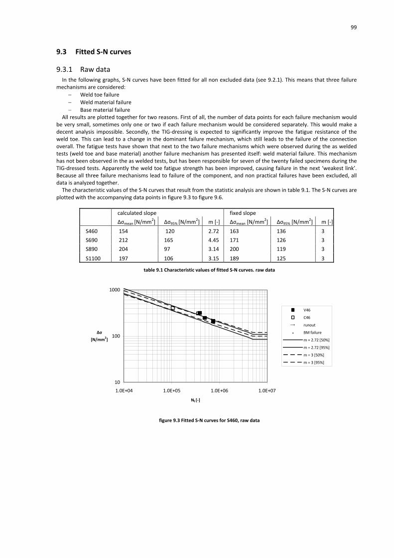
99
9.3 Fitted S‐N curves
9.3.1 Raw data In the following graphs, S‐N curves have been fitted for all non excluded data (see 9.2.1). This means that three failure
mechanisms are considered:
Weld toe failure
Weld material failure
Base material failure All results are plotted together for two reasons. First of all, the number of data points for each failure mechanism would
be very small, sometimes only one or two if each failure mechanism would be considered separately. This would make a decent analysis impossible. Secondly, the TIG‐dressing is expected to significantly improve the fatigue resistance of the weld toe. This can lead to a change in the dominant failure mechanism, which still leads to the failure of the connection overall. The fatigue tests have shown that next to the two failure mechanisms which were observed during the as welded tests (weld toe and base material) another failure mechanism has presented itself: weld material failure. This mechanism has not been observed in the as welded tests, but has been responsible for seven of the twenty failed specimens during the TIG‐dressed tests. Apparently the weld toe fatigue strength has been improved, causing failure in the next ‘weakest link’. Because all three failure mechanisms lead to failure of the component, and non practical failures have been excluded, all data is analyzed together. The characteristic values of the S‐N curves that result from the statistic analysis are shown in table 9.1. The S‐N curves are
plotted with the accompanying data points in figure 9.3 to figure 9.6.
calculated slope fixed slope
Δσmean [N/mm2] Δσ95% [N/mm2] m [‐] Δσmean [N/mm2] Δσ95% [N/mm2] m [‐]
S460 154 120 2.72 163 136 3
S690 212 165 4.45 171 126 3
S890 204 97 3.14 200 119 3
S1100 197 106 3.15 189 125 3
table 9.1 Characteristic values of fitted S‐N curves. raw data
10
100
1000
1.0E+04 1.0E+05 1.0E+06 1.0E+07
Nf [‐]
Δσ
[N/mm2]
V46
C46
runout
* BM failure
m = 2.72 [50%]
m = 2.72 [95%]
m = 3 [50%]
m = 3 [95%]
figure 9.3 Fitted S‐N curves for S460, raw data
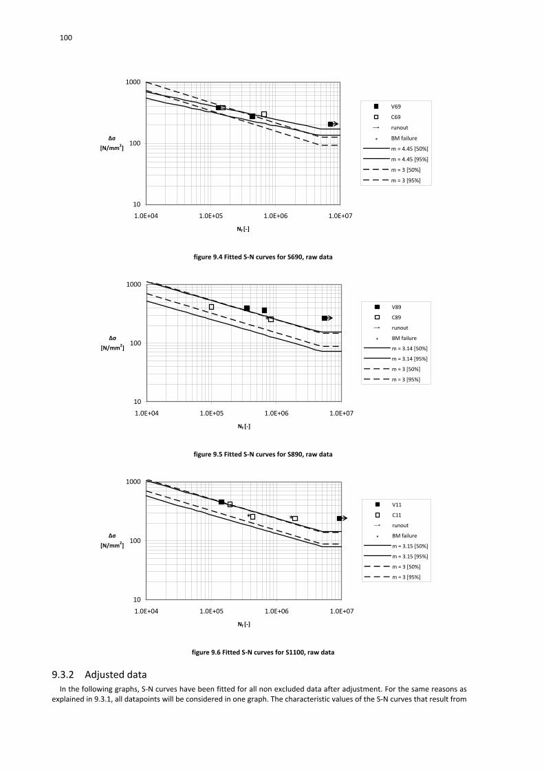
100
10
100
1000
1.0E+04 1.0E+05 1.0E+06 1.0E+07
Nf [‐]
Δσ
[N/mm2]
V69
C69
runout
* BM failure
m = 4.45 [50%]
m = 4.45 [95%]
m = 3 [50%]
m = 3 [95%]
figure 9.4 Fitted S‐N curves for S690, raw data
*
10
100
1000
1.0E+04 1.0E+05 1.0E+06 1.0E+07
Nf [‐]
Δσ
[N/mm2]
V89
C89
runout
* BM failure
m = 3.14 [50%]
m = 3.14 [95%]
m = 3 [50%]
m = 3 [95%]
figure 9.5 Fitted S‐N curves for S890, raw data
* *
10
100
1000
1.0E+04 1.0E+05 1.0E+06 1.0E+07
Nf [‐]
Δσ
[N/mm2]
V11
C11
runout
* BM failure
m = 3.15 [50%]
m = 3.15 [95%]
m = 3 [50%]
m = 3 [95%]
figure 9.6 Fitted S‐N curves for S1100, raw data
9.3.2 Adjusted data In the following graphs, S‐N curves have been fitted for all non excluded data after adjustment. For the same reasons as
explained in 9.3.1, all datapoints will be considered in one graph. The characteristic values of the S‐N curves that result from
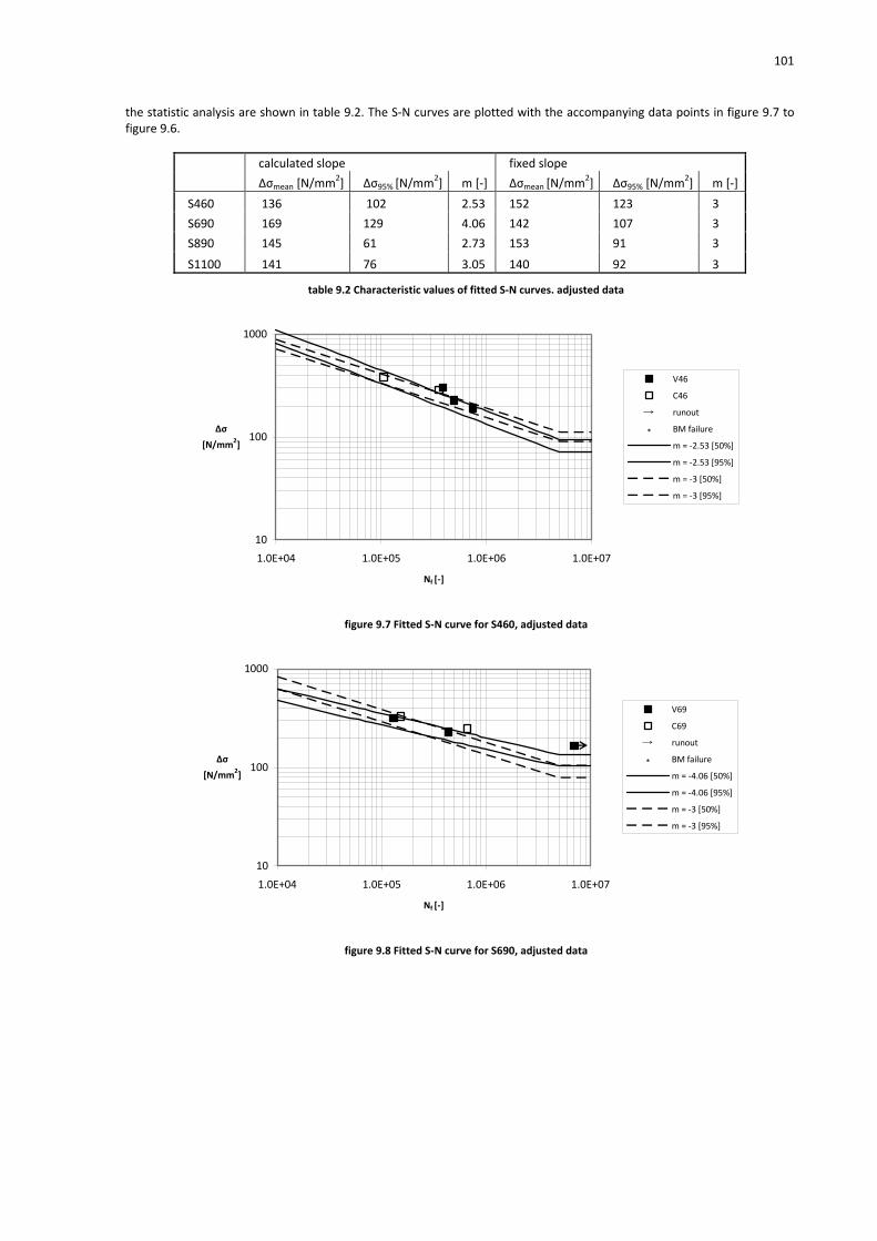
101
the statistic analysis are shown in table 9.2. The S‐N curves are plotted with the accompanying data points in figure 9.7 to figure 9.6.
calculated slope fixed slope
Δσmean [N/mm2] Δσ95% [N/mm2] m [‐] Δσmean [N/mm2] Δσ95% [N/mm2] m [‐]
S460 136 102 2.53 152 123 3
S690 169 129 4.06 142 107 3
S890 145 61 2.73 153 91 3
S1100 141 76 3.05 140 92 3
table 9.2 Characteristic values of fitted S‐N curves. adjusted data
10
100
1000
1.0E+04 1.0E+05 1.0E+06 1.0E+07
Nf [‐]
Δσ
[N/mm2]
V46
C46
runout
* BM failure
m = ‐2.53 [50%]
m = ‐2.53 [95%]
m = ‐3 [50%]
m = ‐3 [95%]
figure 9.7 Fitted S‐N curve for S460, adjusted data
10
100
1000
1.0E+04 1.0E+05 1.0E+06 1.0E+07
Nf [‐]
Δσ
[N/mm2]
V69
C69
runout
* BM failure
m = ‐4.06 [50%]
m = ‐4.06 [95%]
m = ‐3 [50%]
m = ‐3 [95%]
figure 9.8 Fitted S‐N curve for S690, adjusted data

102
*
10
100
1000
1.0E+04 1.0E+05 1.0E+06 1.0E+07
Nf [‐]
Δσ
[N/mm2]
V89
C89
runout
* BM failure
m = 2.67 [50%]
m = 2.67 [95%]
m = 3 [50%]
m = 3 [95%]
figure 9.9 Fitted S‐N curve for S890, adjusted data
* *
10
100
1000
1.0E+04 1.0E+05 1.0E+06 1.0E+07
Nf [‐]
Δσ
[N/mm2]
V11
C11
runout
* BM failure
m = 2.70 [50%]
m = 2.70 [95%]
m = 3 [50%]
m = 3 [95%]
figure 9.10 Fitted S‐N curve for S1100, adjusted data
9.3.3 Discussion Some results show significant deviation from the total dataset (for example, the C89 point near N=1∙105). Some of these
points contain base material failure, but others, such as the example point in figure 9.5, are other mechanisms. Because of the limited size of the dataset it is hard to determine whether these points are indeed a rare exception or part of a widely scattered dataset. Except for the excluded data as described in 9.2.1, no other data points are excluded from the regression in this paragraph or coming paragraphs. The small data set leads to high values of t0,95;n‐f (see 9.2.3), resulting in large difference between the mean and
characteristic curve. This effect is even stronger because of the large influence single data points can have on the standard deviation due to the small sample size. Furthermore, it must be noted that most observed runouts lie greatly above the fatigue limit which is derived from the
value of the fitted S‐N curve at 5∙106 cycles. It is therefore questionable whether the chosen knee point is correct. Due to the limited number of results, especially for Nf>1∙10
6 only a presumption with respect to the knee point can be expressed.
9.4 Comparison
9.4.1 Comparison of data with design codes The connection that was tested, is judged by different design codes in different ways. In table 9.3 the characteristic data
for a given probability of survival (Ps) are shown for the design S‐N curves prescribed by different codes. The design curves are plotted and compared without any further safety factors.

103
Δσc [N/mm2] m [‐] Ps [‐]
Eurocode* 71 3 95.0%
IIW** 92 3 95.0%
NPR‐CEN/TS 13001‐3‐1*** 100 3 97.7%
table 9.3 Characteric values of design S‐N curves for the tested specimens
*Welds checked by NDT from both sides, safety factor not considered. Design curve limited to steels up to Reh=700 N/mm2 ** Welds checked by NDT and misalignment <10% of plate thickness. This criterion is not met in the specimens. Design curve limited to steels up to Reh=900 N/mm2 ***Weld quality B. Detail category for asymmetric butt welds also incorporates asymmetric plate arrangement, which is not the case with the tested specimens. Design curve limited to steels up to Reh=960 N/mm2
When table 9.1, table 9.2 and table 9.3 are compared, it is clear that the very high strength steel specimens (S890 and
S1100) do not always match the codes when the characteristic strengths are compared. However, the characteristic curve value is influenced to a great extent by the uncertainty of the data caused by the small sample size. Below, all data points will be compared with the design lines specified in table 9.3.
Raw data
In figure 9.11 to figure 9.14 the raw data points are compared with the design lines of the different codes and recommendations as specified in table 9.3.
10
100
1000
1.0E+04 1.0E+05 1.0E+06 1.0E+07
Nf [‐]
Δσ
[N/mm2]
V46
C46
runout
* BM failure
EN 1993‐1‐9
IIW recommendations
NPR_CEN/TS 13001‐3‐1
figure 9.11 S460 data points compared with design lines, raw data
10
100
1000
1.0E+04 1.0E+05 1.0E+06 1.0E+07
Nf
Δσ
[N/mm2]
V69
C69
runout
* BM failure
EN 1993‐1‐9
IIW recommendations
NPR‐CEN/TS 13001‐3‐1
figure 9.12 S690 data points compared with design lines, raw data

104
*
10
100
1000
1.0E+04 1.0E+05 1.0E+06 1.0E+07
Nf [‐]
Δσ
[N/mm2]
V89
C89
runout
* BM failure
EN 1993‐1‐9
IIW recommendations
NPR_CEN/TS 13001‐3‐1
figure 9.13 S890 data points compared with design lines, raw data
* *
10
100
1000
1.0E+04 1.0E+05 1.0E+06 1.0E+07
Nf [‐]
Δσ
[N/mm2]
V11
C11
runout
* BM failure
EN 1993‐1‐9
IIW recommendations
NPR‐CEN/TS 130010301
figure 9.14 S1100 data points compared with design lines, raw data
Adjusted results
In figure 9.15 to figure 9.18 the data points after adjustment are compared with the design lines of the different codes and recommendations as specified in table 9.3.
10
100
1000
1.0E+04 1.0E+05 1.0E+06 1.0E+07
Nf [‐]
Δσ
[N/mm2]
V46
C46
runout
* BM failure
EN 1993‐1‐9
IIW recommendations
NPR‐CEN/TS 13001‐3‐1
figure 9.15 S460 data points compared with design lines, adjusted data
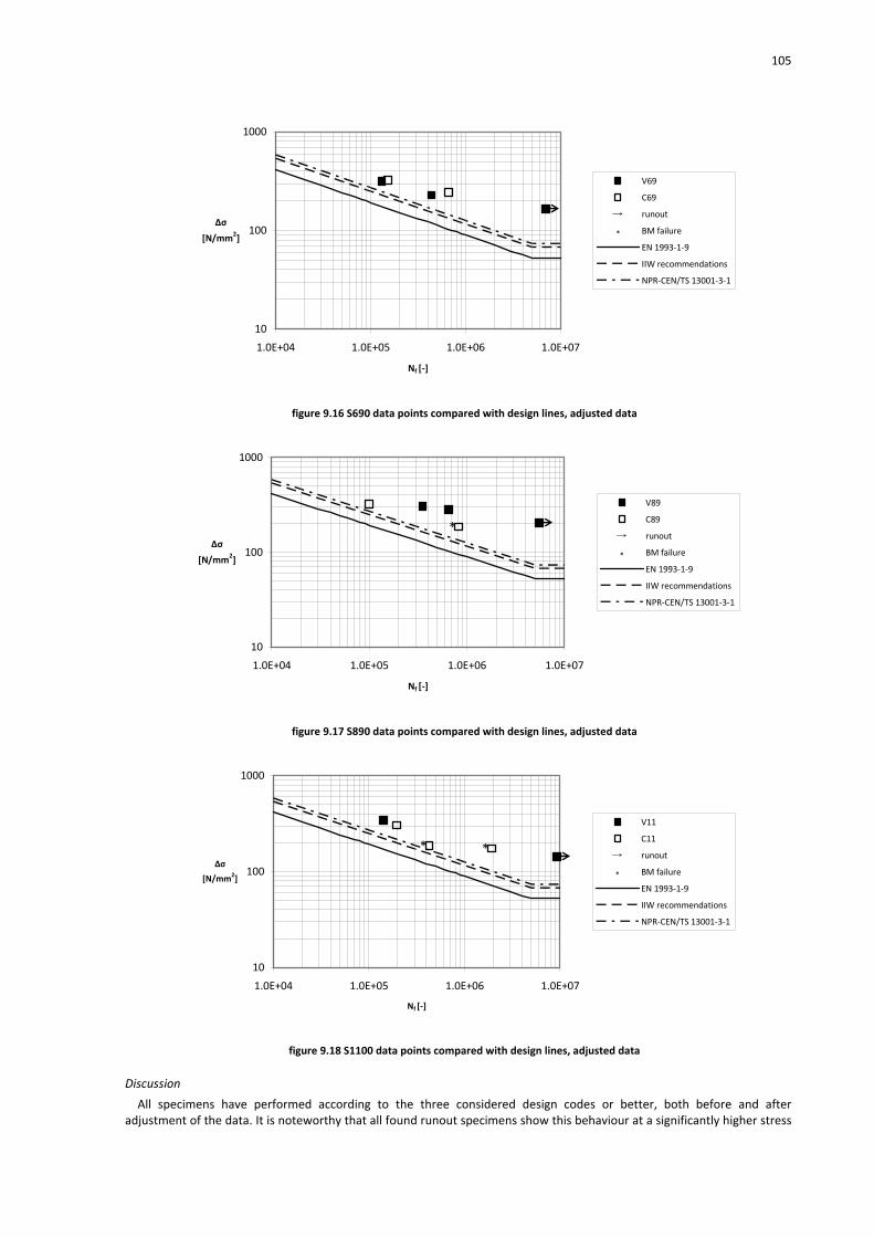
105
10
100
1000
1.0E+04 1.0E+05 1.0E+06 1.0E+07
Nf [‐]
Δσ
[N/mm2]
V69
C69
runout
* BM failure
EN 1993‐1‐9
IIW recommendations
NPR‐CEN/TS 13001‐3‐1
figure 9.16 S690 data points compared with design lines, adjusted data
*
10
100
1000
1.0E+04 1.0E+05 1.0E+06 1.0E+07
Nf [‐]
Δσ
[N/mm2]
V89
C89
runout
* BM failure
EN 1993‐1‐9
IIW recommendations
NPR‐CEN/TS 13001‐3‐1
figure 9.17 S890 data points compared with design lines, adjusted data
* *
10
100
1000
1.0E+04 1.0E+05 1.0E+06 1.0E+07
Nf [‐]
Δσ
[N/mm2]
V11
C11
runout
* BM failure
EN 1993‐1‐9
IIW recommendations
NPR‐CEN/TS 13001‐3‐1
figure 9.18 S1100 data points compared with design lines, adjusted data
Discussion
All specimens have performed according to the three considered design codes or better, both before and after adjustment of the data. It is noteworthy that all found runout specimens show this behaviour at a significantly higher stress

106
range (factor 3‐4 for raw data and a factor 2‐3 for adjusted results) than specified in the design lines. A phenomenon which was also noticed when the data points were compared with the fitted S‐N curves (see 9.3).
9.4.2 Comparison of data with as welded fatigue tests From the TIG‐dressed specimens all non excluded data are considered, for reasons explained in 9.3. In the study by
Pijpers (2011), data were split according to their failure mechanism (base material or weld toe). The arguments to include all data in the analysis which were valid for TIG‐dressed specimens, are not for the as welded data. Therefore, in principle it is only interesting to compare the results of this research with cap weld toe failures from the research by Pijpers. However, all base material failures that were found in this research can be the result of removing the weakest link from the chain by improving the weld toe, but could also already have been the weak link before TIG‐dressing. Therefore, the weld toe failures from the cap side are plotted but also all base material failures are plotted. As was the case for the TIG‐dressed data points, the base material failures will be marked in all diagrams.
Full fatigue life, raw data
In table 9.4 the mean stress range and characteristic stress range at 2∙106 cycles are depicted for the as welded specimens and the TIG‐dressed specimens. A graphic representation of the table can be found in figure 9.19. Although in figure 9.20 to figure 9.23 the TIG‐dressed data points seem to lie in the middle and upper region of the as welded scatter band, the mean and characteristic values in table 9.4 and figure 9.19 do not show a strength increase due to TIG‐dressing in most materials. This strength decrease may be explained by the fact that most as welded specimens were tested under bending, which in general gives better results in fatigue tests (see 9.2.2). The adjusted data therefore may show a different behaviour. The difference between as welded and TIG‐dressed specimens increases when the characteristic stress range is considered for most materials. This can be caused by the fact that a small data set results in more uncertainty of the variation, and therefore results in a lower characteristic stress range. Furthermore, the flattening of the S‐N curve due to TIG‐dressing (see 4.3.4) cannot be observed in most results. Only the steel grade S690 behaves in a way that can be expected, based on literature research: the mean and characteristic strength increase, and the m‐value of the S‐N curve increases.
calculated slope fixed slope
Δσmeanv [N/mm2] Δσ95% [N/mm2] m [‐] Δσmean [N/mm2] Δσ95% [N/mm2] m [‐]
S460 TIG 154 120 2.72 163 136 3
S460 AW 192 165 3.99 171 138 3
S690 TIG 212 165 4.45 171 126 3
S690 AW 193 124 3.68 183 108 3
S890 TIG 204 97 3.14 200 119 3
S890 AW 259 222 6.95 208 138 3
S1100 TIG 197 106 3.15 189 125 3
S1100 AW 169 114 2.56 180 130 3
table 9.4 Comparison of mean and characteristic values at 2∙106 cycles before and after TIG‐dressing, raw data
050100150200250
S460 TIG S460 AW
Δσ
050100150200250
S690 TIG S690 AW
Δσ
050100150200250
S460 TIG S460 AW
Δσ
050100150200250
S690 TIG S690 AW
Δσ
050100150200250
S890 TIG S890 AW
Δσ
050100150200250
S1100 TIG S1100 AW
Δσ
050100150200250
S890 TIG S890 AW
Δσ
050100150200250
S1100 TIG S1100 AW
Δσ
figure 9.19 Graphic overview of table 9.4: mean and characteristic stress range at 2∙106 cycles, raw data

107
10
100
1000
1.0E+04 1.0E+05 1.0E+06 1.0E+07
Nf [‐]
Δσ
[N/mm2]
V46 TIG
C46 TIG
V46 AW
C46 AW
runout
* BM failure
figure 9.20 Comparison between as welded data and TIG‐dressed data, raw data
10
100
1000
1.0E+04 1.0E+05 1.0E+06 1.0E+07
Nf
Δσ
[N/mm2]
V69 TIG
C69 TIG
V69 AW
C69 AW
runout
* BM failure
figure 9.21 Comparison between as welded data and TIG‐dressed data, raw data
*** **
10
100
1000
1.0E+04 1.0E+05 1.0E+06 1.0E+07
Nf [‐]
Δσ
[N/mm2]
V89 TIG
C89 TIG
V89 AW
C89 AW
runout
* BM failure
figure 9.22 Comparison of as welded data and TIG‐dressed data, raw data

108
* * ******
* *
10
100
1000
1.0E+04 1.0E+05 1.0E+06 1.0E+07
Nf [‐]
Δσ
[N/mm2]
V11 TIG
C11 TIG
V11 AW
C11 AW
runout
* BM material
figure 9.23 Comparison of as welded data and TIG‐dressed data, raw data
Full fatigue life, adjusted results
In table 9.5 the mean stress range and characteristic stress range at 2∙106 cycles are depicted for the as welded specimens and the TIG‐dressed specimens after adjustment of the data points. A graphic representation of the table can be found in figure 9.24. In the figure can be seen that still for most materials TIG‐dressing does not seem to provide a significant increase in fatigue strength at 2∙106 cycles, except for steel grade S690. It is remarkable that the fatigue strength increase at 2∙106 cycles of TIG‐dressed specimens seems to become larger when the S‐N curve with a fixed slope is considered (see figure 9.24, right hand side), while a free slope is expected to perform better due to the flattening effect of the S‐N curve (see 4.3.4). This flattening effect is not apparent in the results. When looking at the data points in figure 9.25 to figure 9.28 it is clear that the TIG‐dressed data points generally lie in the upper part of the as welded scatter band with the S1100 data points as possible exception. Because the m‐value of the curves decreases for all results and most data points lie in the region below 1∙106 cycles, the characteristic strength at 2∙106 is strongly influenced. Based on the observations of the scatter plots, at positive effect of TIG‐dressing is likely.
calculated slope fixed slope
Δσmean [N/mm2] Δσ95% [N/mm2] m [‐] Δσmean [N/mm2] Δσ95% [N/mm2] m [‐]
S460 TIG 136 102 2.53 152 123 3
S460 AW 150 127 4.72 127 96 3
S690 TIG 169 129 4.06 142 107 3
S690 AW 144 106 4.72 129 79 3
S890 TIG 145 61 2.73 153 91 3
S890 AW 168 122 3.77 155 106 3
S1100 TIG 141 76 3.05 140 92 3
S1100 AW 112 65 2.14 131 87 3
table 9.5 Comparison of mean and characteristic values at 2∙106 cycles before and after TIG‐dressing, adjusted data

109
050100150200250
S460 TIG S460 AW
Δσ
050100150200250
S690 TIG S690 AW
Δσ
050100150200250
S460 TIG S460 AW
Δσ
050100150200250
S690 TIG S690 AW
Δσ
050100150200250
S890 TIG S890 AW
Δσ
050100150200250
S1100 TIG S1100 AW
Δσ
050100150200250
S890 TIG S890 AW
Δσ
050100150200250
S1100 TIG S1100 AW
Δσ
figure 9.24 Graphic overview of table 9.5: mean and characteristic stress range at 2∙106 cycles, adjusted data
10
100
1000
1.0E+04 1.0E+05 1.0E+06 1.0E+07
Nf [‐]
Δσ
[N/mm2]
V46 TIG
C46 TIG
V46 AW
C46 AW
runout
* BM failure
figure 9.25 Comparison of TIG‐dressed and as welded data, adjusted data
10
100
1000
1.0E+04 1.0E+05 1.0E+06 1.0E+07
Nf [‐]
Δσ
[N/mm2]
V69 TIG
C69 TIG
V69 AW
C69 AW
runout
* BM failure
figure 9.26 Comparison of TIG‐dressed and as welded data, adjusted data

110
*** **
10
100
1000
1.0E+04 1.0E+05 1.0E+06 1.0E+07
Nf [‐]
Δσ
[N/mm2]
V89 TIG
C89 TIG
V89 AW
C89 AW
runout
* BM failure
figure 9.27 Comparison of TIG‐dressed and as welded data, adjusted data
* * ****
*** *
10
100
1000
1.0E+04 1.0E+05 1.0E+06 1.0E+07
Nf [‐]
Δσ
[N/mm2]
V11 TIG
C11 TIG
V11 AW
C11 AW
runout
* BM failure
figure 9.28 Comparison of TIG‐dressed and as welded data, adjusted data
Crack initiation life, raw data
Because TIG‐dressing is expected to influence the crack initiation life to a greater extent than the crack propagation life, the crack initiation lives of the as welded data will be compared with the crack initiation lives of the TIG‐dressed data. No S‐N curves are fitted to the data, but only the overall effect of TIG‐dressing will be discussed. The earlier discussed trend, where the TIG‐dressed data points mainly lie in the middle and upper region becomes
somewhat more distinct in figure 9.29 to figure 9.32. Another way to analyze the effect of TIG‐dressing on the crack initiation time is to compare the average crack initiation life ratios (fNi) of the TIG‐dressed data set and the as welded dataset. In table 9.6 this comparison is made, and based on this table it seems clear that the TIG‐dressing has increased the crack initiation life. An important remark to this table must be made. The specimens tested by Pijpers were provided with three strain gauges at each weld toe, instead of two in this research, but are also wider. If a crack initiates closer to a strain gauge it can be detected earlier. Two strain gauges in Pijpers’ research were placed at the edge of the specimen, where a lot of cracks were found in that research. The results in table 9.6 may be distorted due to these differences, but it is not sure to what extent these geometrical differences between the specimens influence the result.
fNi TIG [‐] fNi AW [‐]
S460 0.70 0.49
S690 0.64 0.40
S890 0.83 0.61
S1100 0.83 0.64
table 9.6 Comparison of fNi of TIG‐dressed specimens and as welded specimens. Runouts are not considered

111
10
100
1000
1.0E+04 1.0E+05 1.0E+06 1.0E+07
Ni [‐]
Δσ
[N/mm2]
V46 TIG
C46 TIG
V46 AW
C46 AW
runout
* BM failure
figure 9.29 Comparison of crack initiation life of TIG‐dressed and as welded data, raw data
10
100
1000
1.0E+04 1.0E+05 1.0E+06 1.0E+07
Ni [‐]
Δσ
[N/mm2]
V69 TIG
C69 TIG
V69 AW
C69 AW
runout
* BM failure
figure 9.30 Comparison of crack initiation life of TIG‐dressed and as welded data, raw data
*** **
10
100
1000
1.0E+04 1.0E+05 1.0E+06 1.0E+07
Ni [‐]
Δσ
[N/mm2]
V89 TIG
C89 TIG
V89 AW
C89 AW
runout
* BM failure
figure 9.31 Comparison of crack initiation life of TIG‐dressed and as welded data, raw data

112
* *****
*** *
10
100
1000
1.0E+04 1.0E+05 1.0E+06 1.0E+07
Ni [‐]
Δσ
[N/mm2]
V11 TIG
C11 TIG
V11 AW
C11 AW
runout
* BM failure
figure 9.32 Comparison of crack initiation life of TIG‐dressed and as welded data, raw data
Crack initiation life, adjusted results
When the adjusted results are considered, the same effect as for raw data can be observed because the crack initiation life ratios are the same. The TIG‐dressed specimens lie in the upper regions of the as welded scatter band. This effect is somewhat clearer than for the adjusted full fatigue life results.
10
100
1000
1.0E+04 1.0E+05 1.0E+06 1.0E+07
Ni [‐]
Δσ
[N/mm2]
V46 TIG
C46 TIG
V46 AW
C46 AW
runout
* BM failure
figure 9.33 Comparison of crack initiation life of TIG‐dressed and as welded data, adjusted data

113
10
100
1000
1.0E+04 1.0E+05 1.0E+06 1.0E+07
Ni [‐]
Δσ
[N/mm2]
V69 TIG
C69 TIG
V69 AW
C69 AW
runout
* BM failure
figure 9.34 Comparison of crack initiation life of TIG‐dressed and as welded data, adjusted data
*
** **
10
100
1000
1.0E+04 1.0E+05 1.0E+06 1.0E+07
Ni [‐]
Δσ
[N/mm2]
V89 TIG
C89 TIG
V89 AW
C89 AW
runout
* BM failure
figure 9.35 Comparison of crack initiation life of TIG‐dressed and as welded data, adjusted data
* ****
***
* *
10
100
1000
1.0E+04 1.0E+05 1.0E+06 1.0E+07
Ni [‐]
Δσ
[N/mm2]
V11 TIG
C11 TIG
V11 AW
C11 AW
runout
* BM failure
figure 9.36 Comparison of crack initiation life of TIG‐dressed and as welded data, adjusted data

114
Discussion
The scatter plots of the raw data show little or no benefit due to TIG‐dressing. When the results are adjusted according to 9.2.2, the effect of TIG‐dressing seems positive, based on observations on the scatter plots. A remark must be made that the used correction factor for the loading mode has been defined as conservative by Pijpers. This means that it is possible that slightly higher fatigue strength should be attributed to the as welded results which were loaded in pure bending. When S‐N curves are fitted to the results, the TIG‐dressed results show a steeper S‐N curve most of the time. Because
most results are located below 1∙106 cycles, this steeper curve results in lower mean and characteristic stress ranges at 2∙106 cycles for TIG‐dressed data when compared with as welded values. When the slope of the S‐N curve is fixed to a value of 3, the results for TIG‐dressed data become less unfavourable, but a clear strength increase can not always be observed. To investigate the possible positive influence of TIG‐dressing in the medium cycle regime, the fitted S‐N curves of both
the as welded data and TIG‐dressed data are plotted in figure 9.37.
S460
10
100
1000
1.0E+04 1.0E+05 1.0E+06 1.0E+07Nf [‐]
Δσ
[N/mm2]
S690
10
100
1000
1.0E+04 1.0E+05 1.0E+06 1.0E+07Nf [‐]
Δσ
[N/mm2]
S890
10
100
1000
1.0E+04 1.0E+05 1.0E+06 1.0E+07Nf [‐]
Δσ
[N/mm2]
S1100
10
100
1000
1.0E+04 1.0E+05 1.0E+06 1.0E+07Nf [‐]
Δσ
[N/mm2]
figure 9.37 Comparison of fitted S‐N curves. Adjusted data, calculated slope.
From figure 9.37 can be concluded that especially in the medium cycle range a beneficial effect due to TIG‐dressing can be observed for most materials. Therefore, the mean and characteristic values of the fitted S‐N curves at N=4∙105 (instead of N=2∙106) are depicted in table 9.7 and figure 9.38. This table and diagram clearly show a mean fatigue strength increase due to TIG‐dressing for materials S460 and S690. The two steel grades which showed a lot of failures in the base material, S890 and S1100 still perform about similar to the as welded specimens. The characteristic values of all steel grades do not always show the results as described above, but this may cohere with the smaller data set of the TIG‐dressed specimens, as explained earlier.
calculated slope fixed slope
Δσmean [N/mm2] Δσ95% [N/mm2] m [‐] Δσmean [N/mm2] Δσ95% [N/mm2] m [‐]
S460 TIG 257 192 2.53 260 210 3
S460 AW 211 178 4.72 217 164 3
S690 TIG 251 191 4.06 243 183 3
S690 AW 203 150 4.72 221 135 3
S890 TIG 261 110 2.73 262 156 3
S890 AW 257 187 3.77 265 181 3
S1100 TIG 239 129 3.05 239 157 3
S1100 AW 238 138 2.14 224 149 3
table 9.7 Comparison of mean and characteristic values at 4∙105 cycles before and after TIG‐dressing, adjusted data

115
050100150200250
S460 TIG S460 AW
Δσ
050100150200250
S690 TIG S690 AW
Δσ
050100150200250
S460 TIG S460 AW
Δσ
050100150200250
S690 TIG S690 AW
Δσ
050100150200250
S890 TIG S890 AW
Δσ
050100150200250
S1100 TIG S1100 AW
Δσ
050100150200250
S890 TIG S890 AW
Δσ
050100150200250
S1100 TIG S1100 AW
Δσ
figure 9.38 Graphic overview of table 9.7: mean and characteristic stress range at 4∙105 cycles, adjusted data
The exceptions to the trend described above are the data from S690 steel. Here, the data points in the scatter plot behave better and the fitted S‐N curves also show a strength increase due to TIG‐dressing at higher cycles (2∙106). The fitted S‐N curve of the TIG‐dressed data has a higher m‐value than the fitted S‐N curve to the as welded data in case of the raw data. When the tabulated fatigue test data are consulted (see Annex C) it can be seen that all failed S690 specimens failed at the weld toe. No base material or weld material failures have been observed in these specimens. Closer inspection of the weld leads to no additional information: the welds in S690 look similar to the welds of S460, where almost only weld material failures occurred. It may be interesting to analyze the geometry of the weld cap with the aid of the already available laser measurement data in future research. Also any changes in residual stress in the weld material may have occurred due to the TIG‐dressing procedure, which, if it concerns a residual stress increase, can lead to worse fatigue behaviour of the weld material than in the as welded case. An opposite trend can be seen in the S1100 specimens. Only one S1100 specimen has failed at the weld toe, and all
others failed in the base material and the S1100 TIG‐dressed data points more or less blend in with the as welded results, especially at high cycles. It may be possible to explain these observations in the following way. TIG‐dressing has improved the weld toe and
removed it as ‘weakest link’ from the chain. For specimens where even after TIG‐dressing the weld toe was the, now stronger, ‘weakest link’, an improvement in fatigue strength can be observed. Specimens which have ‘weak links’ with marginally higher fatigue strength elsewhere in the base material or weld material show only marginal improvement. If the weak link in the as welded specimen was placed outside the weld region, resulting in a base material failure, this will still be the case in the TIG‐dressed situation. In that case, not improvement is observed. In the graphs of the steels that show base material failures, it can be observed that the base material failures indeed blend in with the as welded results, while the rare weld toe or weld material failures lie slightly above the as welded scatter band. The crack initiation life of the TIG‐dressed specimens seems to be improved with respect to the as welded specimens,
resulting in a higher Ni/Nf ratio. However, due to differences in geometry between the TIG‐dressed specimens and the as welded specimens, these results may have been distorted.
9.4.3 Comparison of data with analytical determination of fatigue strength The used analysis method is only valid for the crack initiation life of weld toe cracks. Therefore, only the crack initiation
life of specimens failed at the weld toe and runouts will be compared with the analytical results. This selection results in a relatively limited number of data points which can be compared for the TIG‐dressed case, because several specimens showed other failure mechanisms than a weld toe failure (see 7.3). Furthermore, the analysis method contains corrections for the means stress. The results of the analysis will therefore
only be compared with the results of the tests corrected for means stress, thickness and loading mode.
Comparison of as welded data with model based on peak values of as welded geometry
In figure 9.39 to figure 9.49 the comparison is made between the model as described and derived in chapter 8 and the fatigue test results by Pijpers in the as welded situation. Almost all predicted results lie significantly higher than the test results. Especially the model as derived by Schijve shows very different behaviour than reality. When the knee point in the model by Schijve would be adjusted to 106 cycles (as is recommended for notched, not welded specimens) it would show similar results as the model derived by Hück.

116
10
100
1000
1.0E+04 1.0E+05 1.0E+06 1.0E+07
Ni [‐]
Δσ
[N/mm2]
V46 AW
runout
Schijve (peak)
Schijve (adjusted)
Hück (peak)
Hück (adjusted)
figure 9.39 Comparison of crack initiation life of V46 specimens with weld toe failure and modeled fatigue strength
10
100
1000
1.0E+04 1.0E+05 1.0E+06 1.0E+07
Ni [‐]
Δσ
[N/mm2]
C46 AW
runout
Schijve (peak)
Schijve (adjusted)
Hück (peak)
Hück (adjusted)
figure 9.40 Comparison of crack initiation life of C46 specimens with weld toe failure on cast side and modeled fatigue strength
10
100
1000
1.0E+04 1.0E+05 1.0E+06 1.0E+07
Ni [‐]
Δσ
[N/mm2]
C46 AW
runout
Schijve (peak)
Schijve (adjusted)
Hück (peak)
Hück (adjusted)
figure 9.41 Comparison of crack initiation life of C46 specimens with weld toe failure on rolled side and modeled fatigue strength

117
10
100
1000
1.0E+04 1.0E+05 1.0E+06 1.0E+07
Ni [‐]
Δσ
[N/mm2]
V69 AW
runout
Schijve (peak)
Schijve (adjusted)
Hück (peak)
Hück (adjusted)
figure 9.42 Comparison of crack initiation life of V69 specimens with weld toe failure and modeled fatigue strength
10
100
1000
1.0E+04 1.0E+05 1.0E+06 1.0E+07
Ni [‐]
Δσ
[N/mm2]
C69 AW
runout
Schijve (peak)
Schijve (adjusted)
Hück (peak)
Hück (adjusted)
figure 9.43 Comparison of crack initiation life of C69 specimens with weld toe failure on cast side and modeled fatigue strength
10
100
1000
1.0E+04 1.0E+05 1.0E+06 1.0E+07
Ni [‐]
Δσ
[N/mm2]
C69 AW
runout
Schijve (peak)
Schijve (adjusted)
Hück (peak)
Hück (adjusted)
figure 9.44 Comparison of crack initiation life of C69 specimens with weld toe failure on rolled side and modeled fatigue strength

118
10
100
1000
1.0E+04 1.0E+05 1.0E+06 1.0E+07
Ni [‐]
Δσ
[N/mm2]
V89 AW
runout
Schijve (peak)
Schijve (adjusted)
Hück (peak)
Hück (adjusted)
figure 9.45 Comparison of crack initiation life of V89 specimens with weld toe failure and modeled fatigue strength
10
100
1000
1.0E+04 1.0E+05 1.0E+06 1.0E+07
Ni [‐]
Δσ
[N/mm2]
C89 AW
runout
Schijve (peak)
Schijve (adjusted)
Hück (peak)
Hück (adjusted)
figure 9.46 Comparison of crack initiation life of C89 specimens with weld toe failure on cast side and modeled fatigue strength
10
100
1000
1.0E+04 1.0E+05 1.0E+06 1.0E+07
Ni [‐]
Δσ
[N/mm2]
C89 AW
runout
Schijve (peak)
Schijve (adjusted)
Hück (peak)
Hück (adjusted)
figure 9.47 Comparison of crack initiation life of C89 specimens with weld toe failure on rolled side and modeled fatigue strength

119
10
100
1000
1.0E+04 1.0E+05 1.0E+06 1.0E+07
Ni [‐]
Δσ
[N/mm2]
V11 AW
runout
Schijve (peak)
Schijve (adjusted)
Hück (peak)
Hück (adjusted)
figure 9.48 Comparison of crack initiation life of V11 specimens with weld toe failure and modeled fatigue strength
10
100
1000
1.0E+04 1.0E+05 1.0E+06 1.0E+07
Ni [‐]
Δσ
[N/mm2]
C11 AW
runout
Schijve (peak)
Schijve (adjusted)
Hück (peak)
Hück (adjusted)
figure 9.49 Comparison of crack initiation life of C11 specimens with weld toe failure on cast side and modeled fatigue strength
Comparison of TIG‐dressed data with model based on peak values of TIG‐dressed geometry
In figure 9.50 to figure 9.54 the comparison is made between the model as described and derived in chapter 8 and the fatigue test results in the TIG‐dressed situation. Similarly to the as welded situation, almost all predicted results lie significantly higher than the test results. It seems that the discrepancy between the model and the results is even larger in the TIG‐dressed situation.

120
10
100
1000
1.0E+04 1.0E+05 1.0E+06 1.0E+07
Ni [‐]
Δσ
[N/mm2]
C46 TIG
runout
Schijve (peak)
Schijve (adjusted)
Hück (peak)
Hück (adjusted)
figure 9.50 Comparison of crack initiation life of C46 specimens with weld toe failure on rolled side and modeled fatigue strength
10
100
1000
1.0E+04 1.0E+05 1.0E+06 1.0E+07
Ni [‐]
Δσ
[N/mm2]
V69 TIG
runout
Schijve (peak)
Schijve (adjusted)
Hück (peak)
Hück (adjusted)
figure 9.51 Comparison of crack initiation life of V69 specimens with weld toe failure and modeled fatigue strength
10
100
1000
1.0E+04 1.0E+05 1.0E+06 1.0E+07
Ni [‐]
Δσ
[N/mm2]
C69 TIG
runout
Schijve (peak)
Schijve (adjusted)
Hück (peak)
Hück (adjusted)
figure 9.52 Comparison of crack initiation life of C69 specimens with weld toe failure on rolled side and modeled fatigue strength

121
10
100
1000
1.0E+04 1.0E+05 1.0E+06 1.0E+07
Ni [‐]
Δσ
[N/mm2]
V11 TIG
runout
Schijve (peak)
Schijve (adjusted)
Hück (peak)
Hück (adjusted)
figure 9.53 Comparison of crack initiation life of V11 specimens with weld toe failure and modeled fatigue strength
10
100
1000
1.0E+04 1.0E+05 1.0E+06 1.0E+07
Ni [‐]
Δσ
[N/mm2]
C11 TIG
runout
Schijve (peak)
Schijve (adjusted)
Hück (peak)
Hück (adjusted)
figure 9.54 Comparison of crack initiation life of C11 specimens with weld toe failure on cast side and modeled fatigue strength
Comparison of TIG‐dressed data with model based on peak values of TIG‐dressed geometry and as welded radius
In figure 9.55 to figure 9.59 the comparison is made between the model as described and derived in chapter 8 and the fatigue test results in the TIG‐dressed situation. The results show a similar behaviour as for the previous two comparisons with the model. Because a higher stress concentration factor and fatigue notch factor is attributed to the TIG‐dressed weld toes, the model and actual tests approach each other better than in the previous analysis where only peak values were considered. However, because the as welded results also did not match very well, this is no valid reason to assume that the model with peak values of the TIG‐dressed geometry with an as welded radius is the best model of the TIG‐dressed joint.

122
10
100
1000
1.0E+04 1.0E+05 1.0E+06 1.0E+07
Ni [‐]
Δσ
[N/mm2]
C46 TIG
runout
Schijve (peak)
Schijve (adjusted)
Hück (peak)
Hück (adjusted)
figure 9.55 Comparison of crack initiation life of C46 specimens with weld toe failure on rolled side and modeled fatigue strength
10
100
1000
1.0E+04 1.0E+05 1.0E+06 1.0E+07
Ni [‐]
Δσ
[N/mm2]
V69 TIG
runout
Schijve (peak)
Schijve (adjusted)
Hück (peak)
Hück (adjusted)
figure 9.56 Comparison of crack initiation life of V69 specimens with weld toe failure and modeled fatigue strength
10
100
1000
1.0E+04 1.0E+05 1.0E+06 1.0E+07
Ni [‐]
Δσ
[N/mm2]
C69 TIG
runout
Schijve (peak)
Schijve (adjusted)
Hück (peak)
Hück (adjusted)
figure 9.57 Comparison of crack initiation life of C69 specimens with weld toe failure on rolled side and modeled fatigue strength

123
10
100
1000
1.0E+04 1.0E+05 1.0E+06 1.0E+07
Ni [‐]
Δσ
[N/mm2]
V11 TIG
runout
Schijve (peak)
Schijve (adjusted)
Hück (peak)
Hück (adjusted)
figure 9.58 Comparison of crack initiation life of V11 specimens with weld toe failure and modeled fatigue strength
10
100
1000
1.0E+04 1.0E+05 1.0E+06 1.0E+07
Ni [‐]
Δσ
[N/mm2]
C11 TIG
runout
Schijve (peak)
Schijve (adjusted)
Hück (peak)
Hück (adjusted)
figure 9.59 Comparison of crack initiation life of C11 specimens with weld toe failure on cast side and modeled fatigue strength
Discussion
Almost all test results, both as welded and TIG‐dressed show significant differences with the modelled behaviour. The as welded model seems to perform the best. Both TIG‐dressed models perform a little bit worse, with the peak value model being the least dependable. The sensitivity of the model to slight differences in the weld toe parameters is relatively limited as can be seen from the
figures. The grey lines indicate a varied weld toe to an extent that the bulk of all weld toes are covered (see 8.3), but this only results in a rather small fatigue strength variation. The variation that is found is smaller than a typical fatigue test scatter band (see the figures above). The use of the TIG‐dressed model with the as welded radius instead of all peak values leads to a difference of 13‐20%,
depending on the steel grade. The model predicts a fatigue strength increase due to TIG‐dressing of 30% for S460, which steadily increases to a 52% strength increase for S1100. This fatigue strength increase difference is partly related to the difference in Kf and is partly caused by the assumed higher absolute reduction of residual stresses in higher strength steels. Due to the inaccuracy of the model, it is very hard to rate these numbers at their true value. However, when these values are compared with figure 9.38, it seems that the model overestimates the beneficial effect of TIG‐dressing. To make a good estimation of the validity of the model for the TIG‐dressed specimens, it is important that the as welded
model gives good predictions of the fatigue strength. Because this is not the case, it is very hard to evaluate the accuracy of the TIG‐dressed model. When these issues are set aside and only the relative difference between the as welded model and TIG‐dressed model is considered, it is noticed that the test data lies further beneath the predicted line in the TIG‐dressed situation than in the as welded situation. This is expected to be the other way around, because only the change in geometry

124
and residual stresses is incorporated in the model. The removal of weld flaws should also give a beneficial effect, which should lead to a tested fatigue resistance which is higher than the model. Unfortunately, this is not the case. A remark must be made on the used model to determined Kf. As is explained in 3.5.1, literature recommends the use of
ρ≈a* in the determination of Kf, because this leads to the maximum value of Kf and thus the most conservative result. Because the actual geometry of the weld was measured in this study, the value of the radius to determine Kf was based on these measurements and not on the most conservative value possible. When the radius would be set at this worst case value an increase in Kf would be found, resulting in a lowering of the predicted S‐N curves, thereby increasing the model accuracy. The increase of Kf can vary from a few percent for S460 for more than 30% for S1100. The actual value could not be determined because the a* value of this material is so small, that the accompanying radius has not been modelled. The indication of 30% increase in Kf is based on the smallest radius that has been modelled. However, when this approach would be used, the measurement of the actual weld toe radius is no longer used, which partly eliminates the beneficial effect for the TIG‐dressed specimens. To omit this question, another approach could also be used. It is possible to link the fatigue notch factor to the stress
gradient. This method is related to the highly stressed volume approach as discussed in 3.5.1, but has not been considered in this research. A more thorough analysis of the possibilities to determine Kf, while incorporating the measured weld profile should be subject of further investigation.
9.5 Evaluation of TIG‐dressing influence There are several indications that the TIG‐dressing procedure has had a positive effect on the fatigue strength of the weld
toe. First of all, a new failure mechanism has shown, which was not observed in the as welded specimens tested by Pijpers. Seven of the twenty non‐excluded results showed this new failure mechanism: a crack in the weld material. Whether this is only caused by weld toe improvement, or TIG‐dressing also had influence on the weld material, possibly by increasing residual stresses, may be the subject of further investigation. Other specimens still showed failure at the weld toe, but these data points can mostly be found in the upper regions or above the scatter band of the as welded specimens, thus suggesting a fatigue strength improvement. Finally, some specimens failed in the base material. Whether this base material was already a weak link in the chain before TIG‐dressing or it became the weakest link after the weld toe was improved cannot be proven. However, the scatter plots in 9.4.2 show that the base material failures more or less blend in with the base material results from the as welded tests. This indicates that the observed failure location would also have been the weakest link in an as welded situation. This might be a possible explanation for the relatively poor performance of some the TIG‐dressed specimens of the steel grades S890 and S1100 when compared with the fatigue strength increase of lower strength specimens. Apparently the, very likely improved, weld toe was not the weakest link, even in the as welded situation. One specimen that was excluded from the analysis, specimen V11‐1, may also fall into this category. Here also a base material failure was observed, which would be the weakest link, both in the as welded state and the TIG‐dressed state. The overall trend seems to be an improvement at the weld toe as a result of TIG‐dressing especially in the medium cycle
regime. Clear information on the high cycle regime is not available, due to the scarcity of test data is this regime. Due to other failure mechanisms, not necessarily the whole specimen shows fatigue strength increase. If the weld toe is improved, but the next weak link only behaves marginally better, the TIG‐dressing has limited influence. It must also be noted that the runout test results mostly lie in the upper region of the as welded runouts, but greatly above the fitted fatigue limits or the fatigue limits specified by codes. This is not translated into the fitted S‐N curves, and therefore worth an extra remark. The analytical results do not comply with the test data in a sufficient way to use the developed model to predict the
fatigue strength of components. The test results deviate significantly from the predicted values and the modeled results are non conservative. From the analytical approach it is found that variations of the weld toe parameters within such limits that the bulk of all measured weld toes are covered, have relatively low consequences on the fatigue strength. The differences that are found when such an analysis is made are generally smaller than a typical fatigue test scatter band. To effectively predict the fatigue strength of butt welded specimens, extra research is necessary. Because of the limited number of tests per material and the limited accuracy of the model, this report refrains from
strength increase factors and only the overall trend has been described. For the same reason, and because S890 and S1100 do not show a clear strength improvement as discussed earlier, no material dependent improvement is described. To define strength increase factors for S460 and S690, and to examine whether S890 and S1100 specimens as a whole
show a strength increase more testing is necessary, especially in the high cycle regime.

125
10 Conclusions and recommendations
10.1 Conclusions
10.1.1 Influence of TIG‐dressing of fatigue strength of butt welded specimens
Design codes do not always incorporate a fatigue strength increase due to TIG‐dressing. The fact that all TIG‐dressed specimens show a fatigue strength above the design line of the considered design codes is therefore not surprising.
When the TIG‐dressed specimens are compared with similar as welded specimens, the scatter plots show a trend towards a better fatigue behaviour of the TIG‐dressed specimens for all specimens which have shown failure in the weld area. For steel grades S460 and S690 this concerns almost all specimens. For the higher strength steels a lot of specimens have shown base material failure. Quantitative conclusions cannot be drawn due to the relatively small number of tests.
The materials that have shown base material failures in the as welded condition, S890 and S1100, show little to no improvement of the fatigue strength, because any beneficial effect of the weld toe improvement can only have an effect on specimens that would not have shown base material failure in the as welded condition. The few specimens that have shown weld material failure after TIG‐dressing in these steel grades generally show the above described trend towards fatigue strength improvement.
The failure mechanism in the weld material has become much more prominent. This failure mechanism has only very rarely been observed in the as welded tests, but has been observed on a significant number of the TIG‐dressed specimens. This is a very good indication that the weld toe indeed has been removed as the weakest link from the chain. Whether the weld material is simply the next weak link or has been influenced by TIG‐dressing is not clear.
The main fatigue improvement of TIG‐dressed specimens is expected from improvement of the crack initiation life. When scatter plots of TIG‐dressed and as welded specimens are compared, the difference between the as welded scatter band and the TIG‐dressed specimens seems larger when only the crack initiation life is considered, thus confirming this expectation. It must be noted that differences in geometry of the specimens and instrumentation which were present, can distort this graph because they influence the accuracy with which the crack initiation time can be determined.
10.1.2 Influence of TIG‐dressing on weld geometry of butt welded specimens
As welded weld toe geometries of the considered specimens generally show one geometry variant. When these welds are TIG‐dressed different weld toe geometries can be observed (see figure 6.9). Different variants occur in different frequencies but no single geometry variant dominates the measurements.
The peak value of the distribution of weld toe radii increases from ~1.0 millimeter for as welded specimens to ~3.8 millimeter for TIG‐dressed specimens. The TIG‐dressed results also show a peak in the region of the as welded peak. The spread of weld toe radii increases due to TIG‐dressing.
The peak value of the distribution of weld toe angles decreases from ~27.8° for as welded specimens to ~15.3° for TIG‐dressed specimens. The spread of the data before and after weld toe improvement is similar.
The peak value of the distribution of undercuts is similar for the as welded specimens as for the TIG‐dressed specimens and lies at 0 millimeter. The number of non‐zero undercuts is somewhat larger for the TIG‐dressed specimens. One specific geometry variant shows significantly deeper undercuts than all other considered weld toe geometries, both as welded as TIG‐dressed. This geometry is also consistently associated with a very large weld toe radius and therefore will very likely not be the weakest link in fatigue.
Because the width of the weld is much larger than the influence of TIG‐dressing, the weld improvement has no influence on the weld height. Within one plate specimen the weld height shows only a slight variation. Larger differences in weld height between specimens were found.
The discussed influences, with exception of the undercut influences, lead to an ‘average’ weld toe geometry with a lower stress concentration factor. However, due to the occurrence of a number of smaller weld toe radii in the TIG‐dressed specimens, which is disproportionate with respect to the overall distribution, the theoretical improvement of the fatigue strength is not necessarily as high as is to be expected based on the average improvement.

126
10.1.3 Theoretical influence of changed weld geometry on behaviour of TIG‐dressed specimens
The found spread in the weld geometry data is, based on a sensitivity analysis, not likely to cause a scatter band with the width that is usually associated with fatigue testing.
The fatigue notch factor shows reduction due to TIG‐dressing with slight dependency on the material static strength. Higher strength steels show a greater reduction in fatigue notch factor, due to the difference in the parameter a*. Further differences in fatigue strength improvement due to TIG‐dressing can be sought in other factors, such as residual stress reduction. In the used model in this research the residual stress was assumed to be a fixed fraction of the yield strength, thereby increasing the fatigue strength increase differences between different steel grades
The model shows a reduction of the fatigue notch factor due to the changed weld toe geometry, even if no improvement of the weld toe radius is achieved. This reduction is then mostly caused by a reduction of the weld toe angle.
The model that is used shows poor accuracy for both as welded and TIG‐dressed specimens. Also, the discrepancy between the model and tested specimens is not constant. Any quantitative or qualitative predictions of a fatigue strength increase due to TIG‐dressing can therefore not be expressed.
10.2 Evaluation and recommendations
10.2.1 Assumptions and approximations In this paragraph the main assumptions and approximations will be described so that the conclusions from 10.1 can be
rated at their true value.
All weld toe geometries have been analyzed together, while a few different typical geometries have been observed. One model has been used to represent all TIG‐dressed geometries, leading to an approximation for typical TIG‐dressed geometry type 3 (see figure 6.9).
No probability distribution has been fit to the results of the weld toe parameters. The peak values now have been estimated based on the bar diagrams. Fitting a distribution would make an accurate calculation of the peak value of the distribution possible, but not for all data sets an accurate fit could be made. The accurate calculation of a peak value with a fitted distribution is therefore an illusion.
When analyzing the weld toe geometry, discussion arose as to whether a large notch or a smaller notch inside this main notch should be documented. Based on various arguments, only the main notch was documented.
This research only focuses on the geometrical improvement of TIG‐dressing. Any improvement by removing weld toe flaws is not taken into account. The reduction of residual stresses is approximated, based on literature.
The critical distance approach has not been proven in the finite life region. This research has extended the infinite life that has been determined with this approach into the finite life.
Peterson (1974) has recommended the use of Kf;max when determining the fatigue strength of notched specimens. This research has used the actual measured geometry.
Correction factors for thickness, loading mode, mean stress and residual stress have been acquired from the research by Pijpers (2011). The influence of these factors can also be dependent on the weld toe geometry. In this research the same correction factors as used by Pijpers were used, although it is not certain that these factors will have exactly the same value for TIG‐dressed joints.
Various specimens have shown failure inside the weld material. This failure mechanism was not observed in the as welded joints by Pijpers (2011). Therefore, no correction factors for thickness, loading mode, mean stress and residual stress are available. These cracks have been regarded as weld toe cracks.
10.2.2 Recommendations for further research
Recommendations regarding the TIG‐dressing procedure
At some locations the TIG dressing procedure could not be executed because after grinding gas inclusions appeared. To prevent them from expanding rapidly when heated and possibly ruining the weld, these locations were not TIG‐dressed. It should be investigated whether these gas inclusions would be visible on an X‐ray test, and in what frequency these inclusions appear. Furthermore, it should be investigated whether welds where these inclusions have been observed can be TIG‐dressed without any problems.
Different TIG‐dressed geometries have been observed (see figure 6.9). Only one of these geometries is expected and described by the IIW and other literature. Further research should determine whether these different geometries always occur for butt welded specimens. The welds that were studied in this research were relatively few in number and all executed by one person under the same conditions. To gain a more complete image of the possible geometries, these factors should be varied.

127
Recommendations regarding the laser measurements
All weld geometries have been considered together after the split between as welded and TIG‐dressed was made. When each weld toe parameters and their mutual dependency are recorded and coupled to one of the weld toe variants specified in figure 6.9, the value of the database will increase greatly.
In a lot of weld toe geometries, different notches can be observed. In this study the choice is made to consider only the largest ‘main’ notch, based on a relatively quick assessment of the influence of the smaller notches. Further research should show to what extent these smaller notches influence the fatigue behaviour and should try to match the crack initiation sites on the specimens on any possible local smaller notches which may be present.
In this research a very limited amount of parent material has been incorporated in the research to limit the measuring time. Extending the amount of measured parent material to about 10 millimeter will greatly increase the ability to accurately determine the weld toe angle, weld toe height en undercut, because all these parameters are defined with the parent material as baseline.
A number of specimens have failed in the weld material. Although data is available of this area of the weld, the exact geometry of any present notches has not been determined. To accurately model these failures, this area of the weld should be analyzed thoroughly. This analysis may also lead to an explanation of the fact that the S460 specimens have shown a lot of weld material failures and the S690 specimens have none while they have, to the eye, a similar weld material geometry.
Recommendations regarding the fatigue testing
To avoid runouts, most specimens were tested at relatively high stresses. This leads to an uncertain determination of the slope of the S‐N curve. More tests should be done at lower stress ranges leading to failure at higher cycles
A high uncertainty exists in the variation of the dataset due to the limited number of data points per steel grade. Additional testing should give more certainty of the actual scatter band of the TIG‐dressed results.
Recommendations regarding the modelling and adjustment of the fatigue strength
In this research an assumption was made concerning the reduction of residual stresses at the weld toe before and after TIG‐dressing. Additional research on residual stresses in TIG‐dressed butt welded joints is necessary to accurately model a fatigue strength increase. The residual stresses in the weld material are also interesting to measure, because an increase of residual stresses in the weld material may explain the occurrence of the extra failure mechanism in the weld material.
When the weld toe geometries have been analyzed more thoroughly as described above, it may be possible to determine a worst case scenario by combining different weld toe parameters according to their actual occurrence and dependencies. This can lead to an accurate worst case value of Kf.
All correction factors for thickness, mean stress and loading mode have been based on the research by Pijpers (2011). The influence of some factors depends on the weld geometry as well. Further research should investigate whether the used correction factors are also valid for TIG‐dressed geometries or define new correction factors.
All correction factors for thickness, mean stress and loading mode have been based on the research by Pijpers (2011). Because in the research by Pijpers no weld material failures were observed, no such correction factors were available for the current research. Additional research should focus on correction factors when failure is observed in the weld material.
The developed model of the fatigue strength is inaccurate. Due to assumptions made when applying the critical distance approach, the determination of Kf may be less precise, leading to a less accurate model. Omitting these assumptions may improve model accuracy but will partly neutralize the beneficial geometrical influence of TIG‐dressing. Other methods to determine the fatigue notch factor, such as the stress gradient approach, may also lead to better results.
Recommendations regarding unused data of crack monitoring and hardness measurements
The crack monitoring data which is presented in Annex I, has not been analyzed. Although limited, this database may give insight into any influences of the TIG‐dressing procedure on the crack propagation life when combined with similar measurements on as welded specimens from Pijpers (2011). This calculation could also be used to verify the measured number of cycles to crack initiation.
The hardness measurements show rather different results than found in literature. Based on observations, interesting conclusions can be drawn if a relation can be made between hardness and fatigue strength. A more thorough research of more TIG‐dressed specimens can lead to more conclusive results.

128

129
Annex A: References
[1] Anami, K and Miki, C. ‘Fatigue strength of welded joints made of high‐strength steels’, Progress in Structural Engineering and Materials, Vol. 3, pp. 86‐94, 2001
[2] Anthes, R.J. Volker Kottgen, V.B. Seeger, T. ‘Kerbformzahlen von Stumpfstößen und Doppel‐T‐stößen’, Schweißen und schneiden, vol. 45 no. 12 pp. 685‐688, 1993
[3] Brozzetti, J., Hirt, M. A., Ryan, I. Sedlacek, G. Smith, I.F.C. ‘BAckbround information on fatigue design rules – Statistical evaluation’ Chapter 9, document 9.01, Eurocode 3 Editorial group, 1989
[4] Dahle, T. ‘Design fatigue strength of TIG‐dressed welded joints in high‐strength steels subjected to spectrum loading’, International Journal of Fatigue, Vol. 20, No. 9, pp. 677‐681, 1998
[5] EngineeringArchives.com, 2008 [6] ESDEP – Lecture WG12: Fatigue [7] FME‐CWM – Constructiestaalsoorten met hoge sterkte, VM‐publication 125, 2008 [8] Gudehus, H. Zenner, H. ‘Leitfaden fur Betriebsfestigkeitsrechnung’, Verlag Stahleisen GmbH, 1999 [9] Gurney, T.R. ‘Fatigue of welded structures’, Cambridge University Press, 1979 [10] Haagensen, P.J. and Maddox, S.J. ‘IIW Recommendations on Post Weld Improvement of Steel and Aluminium
Structures, IIW document XIII‐1815‐00, 2001 [11] Haagensen, P.J. Drågen, A. Slind, T. and Ørjasæter, O. ‘Prediction of the improvement in fatigue lif of welded
joints due to grinding, TIG dressing, weld shape control and shot peening’, Proceedings of the 3rd International ECSC Offshore Conference on Steel in Marine Structures (SIMS ’87), Delft, 1987
[12] Haibach, E. ‘Betriebsfestigkeit – Verfahren und Daten zur Bauteilberechnung’, Springer‐Verlag, 2006 [13] Hildebrand, J. Starcevic, I. Werner, F. Heinemann, H. and Köhler, G. ‘Numerical simulation of TIG‐dressing of
welded joints’ Joint International Conference on Computing and Decision Making in Civil and Building Engineering, Montréal, 2006
[14] Hobbacher, A. ‘Recommendations for fatigue design of welded joints and components, IIW document XIII‐2151‐07/XV‐1254‐07, 2007
[15] Hück, M., Thrainer, L., Schütz, W. ‘Berechnung von Wöhlerlinien fur Bauteile aus Stahl, Stahlguss und Grauguss – Synthetische Wöhlerlinien’, Bericht Nr. ABF 11 (Zweite Überarbeitete Fassung), Verlag Stahleisen, 1981
[16] Huo, L. Wang, D. Zhang, Y. ‘Investigation of the fatigue behaviour of the welded joints treted by TIG dressing and ultrasonic peening under variable‐amplitude load’, International Journal of Fatigue, Vol. 27 pp. 95‐101, 2005
[17] Janssen, M. Zuidema, J. Wanhill, R.J.H. ‘Fracture Mechanics’, Delft University Press, 2002 [18] Kuguel, R. ‘A relation between theoretical stress concentration factor and fatigue notch factor deduced from the
concept of highly stressed volume’, Proceedings of ASTM 61, 732‐744, 1961 [19] Lopez Martinez, L. Lin, R. Wang, and Blom, A.F. ‘Investigation of residual stresses in as‐welded and TIG‐dressed
specimens to static/spectrum loading’ Proceedings of NESCO: “Welded High‐Strength Steel Structures”, Stockholm, 1997
[20] Maddox, S.J. ‘Fatigue strength of welded structures’, Abington Publishing, 1991 [21] NEN‐EN 1993‐1‐9, Eurocode 3: Design of steel structures – Part 1‐9: Fatigue, 2006 [22] NEN‐EN 1993‐1‐12, Eurocode 3: Design of steel structures – Part 1‐12: Additional rules for the extension of EN
1993 up to steel grades S700, 2007 [23] NEN‐EN‐ISO 5817, Welding – Fusion welded joints in steel, nickel, titanium and their alloys (beam welding
excluded) – Quality levels for imperfections,2007 [24] Neuber H. ‘Kerbspannungslehre’, Springer Verlag, 1937 [25] Neuber H. ‘Theory of Notch Stresses’, Ann Arbor Mich, 1946 [26] Neuber H. ‘Über die Berücksichtigung der Spannungskonzentration bei Festigkeitsberechnungen’, Konstruktion,
Vol 20, No. 7, pp. 245‐251, 1968 [27] NPR‐CEN/TS 13001‐3‐1, Cranes – General Design – Part 3‐1: Limit states and proof of competence of steel
structures, 2005 [28] Pedersen, M.M. Mouritsen, O.Ø. Hansen, M.R. and Andersen J.G. ‘Experience with the Notch Stress Approach for
Fatigue Assessment of Welded Joints’ Proceedings of the Swedish Conference on Light Weight Optimized Welded Structures, Borlänge, 2010
[29] Pedersen, M.M. Mouritsen, O.Ø. Hansen, M.R. Andersen J.G and Wenderby, J. ‘Comparison of Post Weld Treatment of High Strength Steel Welded Joints in Medium Cycle Fatigue’, IIW document XIII‐2272‐09, 2009
[30] Peterson, R.E. ‘Stress concentration factors’, New York, John Wiley, 1974 [31] Pijpers, R.J.M. Kolstein, M.H. Romeijn, A. and Bijlaard, F.S.K. ‘Fatigue experiments on very high strength steel
base material and transverse butt welds’, Advanced steel construction, Vol, 5, No. 1, 14‐32, 2009 [32] Pijpers, R.J.M. Kolstein, M.H. ‘Fatigue strength of truss girders made of Very High Strength Steel’, as presented
on the: 13th International Symposium on Tubular Structures, pp. 499‐505, 2010

130
[33] Pijpers, R.J.M. ‘Fatigue strength of welded connections made of very high strength cast and rolled steels’, Dissertation, M2I, 2011
[34] Radaj, D. Sonsino, C.M. and Fricke, W. ‘Fatigue assessment of welded joints by local approaches – second edition’, Woodhead publishing limited, 2006
[35] Romeijn, A. ‘Lecture notes CT5126 – Fatigue’, Delft University of Technology, 2006 [36] Siebel, E. and Stieler, M., ‘Ungleichförmiche Spannungsverteilung bei schwingender Beanspruchug’, VDI‐
Zeitschrift, Vol. 97, No. 5, pp. 121‐126, 1993 [37] Schijve, J. ‘Fatigue of Structures and Materials’, Kluwer Academic Publishers, 2001, [38] Sonsino, C.M., ‘Zur Bewertung des Schwingfestigheitsverhaltens von Bauteilen mit Hilfe örtlicher
Beanspruchungen’, Konstruktion, 1993, Vol. 45, pp. 25‐33, 1993 [39] Tricoteaux, A. Fardoun, F. Degallaix, S. Sauvage, F. ‘Fatigue crack initiation life prediction in high strength
structural steel welded joints’, Fatigue and Fracture of Engineering Materials, Vol. 18, No. 2 pp. 189‐200, 1995 [40] Wanhill, R.J.H. ‘Durability analysis using short and long fatigue crack growth data’, Proceedings of the
International Conference on Aircraft Damage Assessment and and Repair, Melbourne, 1991 [41] Wortel, H van. ‘Integrity of High Strength Steel Structures; Final Report of Work Package: Fabrication’, TNO
Report, 2006

131
Annex B: Test specimens
On the following pages the geometry of the produced test specimens will be depicted. The geometry of tested specimens is tabulated for each specimen separately. The figure below gives guidance to the
location of the various measurements.

132
W1
W2
W3
W4
WL1
WL2
M1
M2
T1
T2
T3
T4
T5
T6
T7
T8
Side 1
Side 2
V46‐1
99‐100
70
70
100‐101
49
51
7.7
7.4
25.4
25.3
25.3
25.1
25.3
25.1
25.5
25.7
Rolled
Rolled
V46‐2
99‐101
70
70
100‐101
50
51
8.0
8.3
25.5
25.6
25.3
25.2
25.3
25.4
25.5
25.5
Rolled
Rolled
V46‐3
101‐103
70
70
102‐106
51
49
8.0
7.7
25.5
25.6
25.2
25.1
25.3
25.1
25.5
25.4
Rolled
Rolled
V69‐1
102‐106
70
70
101‐102
45
48
4.8
4.3
24.6
24.6
24.5
24.5
24.4
24.5
24.6
24.6
Rolled
Rolled
V69‐2
103‐106
70
70
104‐105
44
46
6.1
6.7
24.6
24.6
24.4
24.5
24.5
24.4
24.6
24.7
Rolled
Rolled
V69‐3
104‐109
70
70
107‐111
45
43
6.7
6.7
24.8
25.0
24.6
24.6
24.6
24.7
24.7
24.7
Rolled
Rolled
V89‐1
93‐97
70
70
98‐100
44
45
3.9
4.1
24.6
24.6
24.6
24.7
24.7
24.6
24.9
24.7
Rolled
Rolled
V89‐2
98‐99
70
70
91‐98
42
42
4.2
3.8
24.7
24.7
24.6
24.6
24.7
24.7
24.7
24.7
Rolled
Rolled
V89‐3
99‐100
70
70
101‐104
44
42
3.8
3.2
24.7
24.7
24.6
24.5
24.6
24.6
24.7
24.7
Rolled
Rolled
V11‐1
98‐99
70
70
98‐99
39
38
2.7
2.3
19.9
20.0
20.0
20.0
19.8
19.8
19.9
19.9
Rolled
Rolled
V11‐2
102‐103
70
70
92‐103
35
36
5.0
4.6
20.0
20.0
20.1
19.9
20.0
19.9
20.1
20.0
Rolled
Rolled
V11‐3
104‐106
70
70
102‐105
30
32
4.3
4.3
20.1
20.1
19.8
20.0
19.8
19.8
20.0
19.9
Rolled
Rolled
C46
‐1
104‐109
70
70
100‐101
51
51
9.6
7.7
25.5
25.6
25.5
25.4
27.1
27.0
27.0
27.1
Rolled
Cast
C46
‐2
C46
‐3
105
70
70
105‐111
49
49
8.4
6.5
25.4
25.5
25.1
25.1
26.9
27.2
28.1
29.1
Rolled
Cast
C69
‐1
106
70
70
107‐112
53
51
7.1
8.5
26.0
25.7
26.0
25.9
24.7
24.7
24.7
24.7
Cast
Rolled
C69
‐2
103‐105
70
70
102‐103
49
51
6.4
7.6
26.0
25.9
25.6
25.6
24.5
24.6
24.7
24.7
Cast
Rolled
C69
‐3
105‐108
70
70
104‐105
48
48
8.4
7.4
24.7
24.5
24.4
24.5
25.4
25.4
25.7
25.3
Rolled
Cast
C89
‐1
102‐103
70
70
102‐104
44
44
? ?
24.3
24.8
24.4
24.6
24.4
24.5
24.5
24.6
Rolled
Cast
C89
‐2
103‐104
70
70
97‐98
45
44
3.3
3.0
24.7
24.7
24.4
24.6
24.3
24.4
23.7
23.7
Rolled
Cast
C89a‐1
104‐105
70
70
101‐106
45
44
4.3
3.2
24.8
24.9
24.7
24.7
23.9
23.9
23.7
24.1
Rolled
Cast
C11
‐1
98
70
70
97‐99
43
42
3.5
3.4
20.2
20.1
20.0
20.1
20.9
20.9
21.3
21.2
Rolled
Cast
C11
‐2
99‐100
70
70
100‐101
40
44
2.5
2.4
20.0
20.1
20.0
20.0
20.8
20.7
21.2
21.0
Rolled
Cast
C11
‐3
97‐99
70
70
97‐100
41
41
1.1
1.0
20.0
20.0
20.0
20.1
20.5
20.3
20.7
20.7
Rolled
Cast
Remarks:
―
All measurements in
millim
eters
―
C46‐2: b
ent due to test rig error
―
C69‐2: w
eld root is ground smooth due to lack of TIG dressing
―
C89‐2: large defects are rem
oved and filled in
with weld m
aterial. Specim
ens is, even after treatmen
t, not en
tirely defect free,
based
on visual inspection

133
Crack location
ΔσN
R (SG
)R (F)
ΔσN/R based
on SG
Ni
Np
Nf
Ni/NfΔσ (F/A)
Km
f Ni
f Np
f lm;Nf
f lm;Nif lm
;Np
f t;Nf
f t;Ni
f t;Np
f mV46‐1
WM_cap
_middle
319
0.53
0.026
3272796
115256
388052
0.70
230
1.39
0.70
0.30
1.06
1.05
1.08
1.00
1.00
1.00
1.00
V46‐2
WM_cap
_middle
248
0.39
0.035
2,3,4,5
379602
115306
494908
0.77
173
1.43
0.77
0.23
1.06
1.05
1.09
1.00
1.00
1.00
0.97
V46‐3
WM_cap_edge
212
0.43
0.035
3,5
603819
139011
742830
0.81
146
1.46
0.81
0.19
1.06
1.06
1.09
1.00
1.00
1.00
0.96
V69‐1
N/A
206
0.33
0.042
4,5
7023317
07023317
1.00
147
1.40
1.00
0.00
1.05
1.05
1.08
1.01
1.01
1.00
0.85
V69‐2
WT_rolled_cap
_middle
277
0.31
0.028
4,5
340765
98795
439560
0.78
206
1.34
0.78
0.22
1.05
1.04
1.07
1.01
1.01
1.00
0.87
V69‐3
WT_rolled_cap
_middle
380
0.28
0.023
347494
83790
131284
0.36
264
1.44
0.36
0.64
1.08
1.05
1.09
1.00
1.01
1.00
0.90
V89‐1
WM_cap
_middle
364
0.20
0.022
2,3,5
594172
60242
654414
0.91
290
1.26
0.91
0.09
1.04
1.04
1.06
1.00
1.00
1.00
0.81
V89‐2
N/A
266
0.22
0.032
2,3,4,5
5551351
05551351
1.00
215
1.24
1.00
0.00
1.03
1.03
1.05
1.00
1.00
1.00
0.79
V89‐3
WM_cap
_middle
394
0.13
0.023
4,5
250389
102673
353062
0.71
325
1.21
0.71
0.29
1.04
1.03
1.05
1.00
1.01
1.00
0.81
V11‐1
BM_rolled_root_ed
ge181
0.23
0.118
12
190258
48657
238915
0.80
225
0.80
0.80
0.20
1.00
1.00
0.98
1.00
1.00
1.00
0.68
V11‐2
WT_rolled_cap
_middle
452
0.46
0.026
2,3
95083
47420
142503
0.67
325
1.39
0.67
0.33
1.06
1.05
1.08
1.06
1.09
1.00
0.86
V11‐3
N/A
240
0.19
0.043
2,3,4,5
9270063
09270063
1.00
176
1.36
1.00
0.00
1.05
1.05
1.08
1.10
1.10
1.00
0.69
C46‐1
WM_cap
_middle
309
0.49
0.027
2291148
65672
356820
0.82
213
1.45
0.82
0.18
1.06
1.05
1.09
0.99
0.99
1.00
0.98
C46‐2
C46‐3
WT_rolled_cap
_middle
408
0.55
0.023
2,3
41827
64209
106036
0.39
273
1.49
0.39
0.61
1.08
1.06
1.10
1.00
1.00
1.00
1.02
C69‐1
WT_rolled_cap
_middle
380
0.32
0.026
494509
58278
152787
0.62
280
1.36
0.62
0.38
1.06
1.05
1.08
1.00
1.00
1.00
0.91
C69‐2
WT_rolled_cap
_middle
298
0.32
0.032
4523670
141806
665476
0.79
198
1.51
0.79
0.21
1.07
1.06
1.10
1.01
1.01
1.00
0.88
C69‐3
WT_rolled_root_middle
124
8.67
0.036
8,9,10,11
3073539
118434
3191973
0.96
171
0.73
0.96
0.04
0.94
0.94
0.91
1.01
1.01
1.00
0.75
C89‐1
BM_cast_side
254
2,8
795902
30714
826616
0.96
1.00
1.00
1.00
1.00
1.00
1.00
0.73
C89‐2
BM_cast_cap_m
iddle
228
0.25
0.025
6 (*70/98)
54419
51952
106371
0.51
236
0.97
0.51
0.49
1.00
1.00
1.00
1.00
1.00
1.00
0.78
C89a‐1
WM_cap
_middle
411
0.16
0.017
2,3,4,5
73659
25651
99310
0.74
342
1.20
0.74
0.26
1.03
1.03
1.05
1.01
1.01
1.00
0.82
C11‐1
BM_cast_cap_edge
254
0.13
0.032
3375344
55472
430816
0.87
218
1.16
0.87
0.13
1.00
1.00
1.01
1.00
1.00
1.00
0.74
C11‐2
BM_cast_cap_edge
238
61854793
65302
1920095
0.97
1.00
1.00
1.01
1.00
1.00
1.00
0.74
C11‐3
WT_cast_cap
_edge/(BM_cast_cap_edge)
412
0.27
0.130
5154896
39490
194386
0.80
344
1.20
0.80
0.20
1.03
1.03
1.05
1.07
1.08
1.00
0.81
Rerun specim
ens
Crack location
ΔσN
R (SG
)R (F)
ΔσN/R based
on SG
Ni
Np
Nf
Ni/NfΔσ (F/A)
Km
f Ni
f Np
f lm;Nf
f lm;Nif lm
;Np
f t;Nf
f t;Ni
f t;Np
f mΔσN at SG
of final failure
C11‐2
IBM_cast_cap_edge
177
0.09
0.048
6 (*70/100)
724750
107147
831897
0.87
147
1.20
0.87
0.13
1.00
1.00
1.01
1.00
1.00
1.00
0.71
253
C11‐2
IIBM_cast_cap_edge
225
0.287
0.034
61022896
65302
1088198
0.94
228
0.99
0.94
0.06
1.00
1.00
1.00
1.00
1.00
1.00
0.75
225
C11‐2
eq
BM_cast_cap_edge
238
61854793
65302
1920095
0.97
1.00
1.00
1.01
1.00
1.00
1.00
0.74
C8
9-1
IBM_cast_root_middle
157
‐0.24
0.025
12 (*70/103)
633167
113271
746438
0.85
157
1.00
0.85
0.15
1.00
1.00
1.00
1.00
1.00
1.00
0.73
248
C8
9-1
IIBM_cast_side_ed
ge299
0.038
0.025
2,8
49464
30714
80178
0.62
268
1.12
0.62
0.38
1.00
1.00
1.01
1.00
1.00
1.00
0.77
299
C89‐1
eq
BM_cast_side_edge
254
2,8
795902
30714
826616
0.96
1.00
1.00
1.00
1.00
1.00
1.00
0.73
Annex C: Fatigue test data

134

135
Annex D: Material certificates

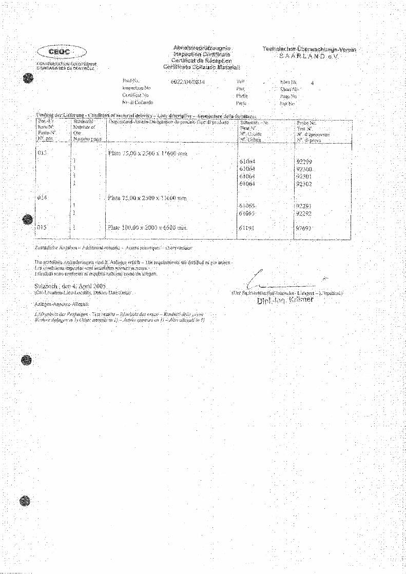


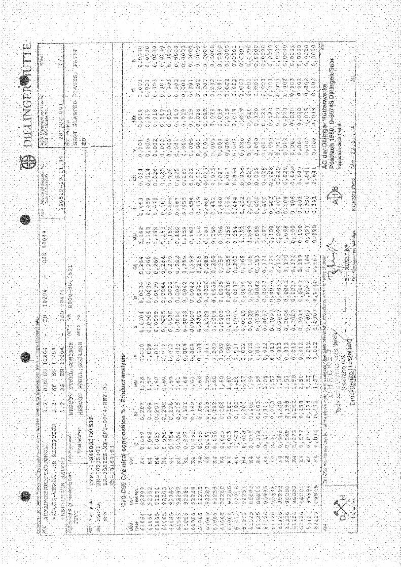


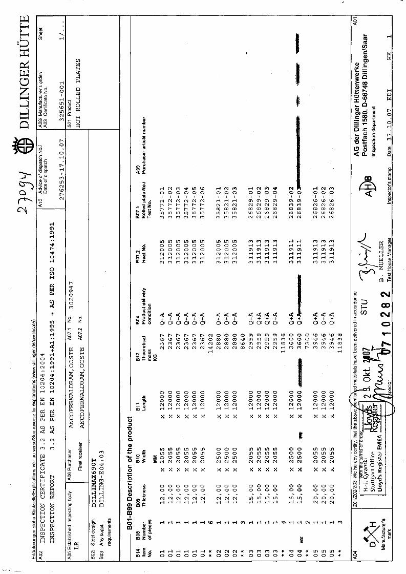
Erla
uter
unqe
nsi
ehe
Ruc
ksel
te/E
xptic
atlo
nsvo
irau
vers
o/S
eere
vers
efo
rexc
lana
tlons
Iww
w.d
illin
oer.
de/c
ertif
icat
e)D
ILL
ING
ER
HU
TT
EA
02IN
SP
EC
TIO
NC
ER
TIF
ICA
TE
3.2
AS
PER
EN
10
20
4:2
00
4
INS
PE
CT
ION
RE
POR
T3
.2A
SPE
RE
N1
02
04
:19
91
+A
l:1
99
5+
AS
PER
ISO
10
47
4:1
99
1
A10
Adv
ice
ofdi
spat
chN
o.1
Dat
eof
disp
atch
27
62
53
-17
.10
.07
A081
Man
ufac
ture
r'sor
derl
A03
Cer
tific
ate
No.
32
56
51
-00
1
She
et
11..
.A
05E
stab
lishe
dIn
spec
ting
body
LR
A06
Pur
chas
er
Fin
alre
ceiv
er
AN
CO
FER
WA
LD
RA
M,O
OST
E
AN
CO
FER
WA
LD
RA
M,O
OST
E
A07
.1N
o.
A07
.2N
o.
30
20
94
7B
01P
rodu
ct
HO
TR
OL
LE
DPL
AT
ES
B021
Ste
elde
sign
.
B03
Any
supp
l.
requ
irem
ents
DIL
LlM
AX
69
0T
DIL
LIN
G-E
04
:03
B01
·B99
De
scri
pti
on
oft
hep
rod
uct
B14
B08
B09
B10
B11
B12
B04
B07
.2B
07.1
A09
Item
Nu
mb
er
Th
ickn
ess
Wid
thLe
ngth
Th
eo
retic
al
Pro
du
ctd
eliv
ery
Hea
tNo.
Rol
led
plat
eN
o.1
Pu
rch
ase
ra
rtic
len
um
be
rN
o.o
fpi
eces
mas
sco
nd
itio
nT
est
No.
MM
KG
01
11
2,0
0X
20
55
X1
20
00
23
67
Q+
A3
12
00
53
57
72
-01
01
11
2,0
0X
20
55
X1
20
00
23
67
Q+
A3
12
00
53
57
72
-02
01
11
2,0
0X
20
55
X1
20
00
23
67
Q+
A3
12
00
53
57
72
-03
01
11
2,0
0X
20
55
X1
20
00
23
67
Q+
A3
12
00
53
57
72
-04
01
11
2,0
0X
20
55
X1
20
00
23
67
Q+
A3
12
00
53
57
72
-05
01
11
2,0
0X
20
55
X1
20
00
23
67
Q+
A3
12
00
53
57
72
-06
**6
14
20
202
11
2,0
0X
25
00
X1
20
00
28
80
Q+
A3
12
00
53
58
21
-01
021
12
,00
X2
50
0X
12
00
02
88
0Q
+A
31
20
05
35
82
1-0
202
11
2,0
0X
25
00
X1
20
00
28
80
Q+
A3
12
00
53
58
21
-03
**3
86
40
.0
31
15
,00
X2
05
5X
12
00
02
95
9Q
+A
31
19
13
26
82
9-0
103
11
5,0
0X
20
55
X1
20
00
29
59
Q+
A3
11
91
32
68
29
-02
031
15
,00
X2
05
5X
12
00
02
95
9Q
+A
31
19
13
26
82
9-0
303
11
5,0
0X
20
55
X1
20
00
29
59
Q+
A3
11
91
32
68
29
-04
**4
11
83
604
11
5,0
0X
25
00
X1
20
00
36
00
Q+
A3
11
91
12
68
39
-02
04~
11
5,0
0X
25
00
.-X
12
00
0-e
36
00
Q+
.w.$
$l1
I3
11
91
12
68
39
-03
,r
I.~
h"
t~
'.**
27
20
00
51
20
,00
X2
05
5X
12
00
03
94
6Q
+A
31
19
13
26
82
6-0
10
51
20
,00
X2
05
5X
12
00
03
94
6Q
+A
31
19
13
26
82
6-0
205
12
0,0
0X
20
55
X1
20
00
39
46
Q+
A3
11
91
32
68
26
-03
**3
11
83
8
-A
04Z0
11Z0
2/Z0
3W
ehe
reby
cert
ify.t
hatt
heaboveJflenti~1
mat
eria
lsha
vebe
ende
liver
edin
acco
rdan
ceA
Gd
er
Dill
ing
er
Hu
tte
nw
erk
eA
01
;;-~
_ly"
:'.~
ik'r
'~or
o.~~
2.
Okl
.~
ST
Ul'r
/!'-
ABa
DXH
Po
stfa
ch15
80,D
·667
48D
illin
ge
n/S
aa
rS
tutt
gart
Off
ice
a.~rer
Insp
ect
ion
de
pa
rtm
en
t
Lloy
d's
Regi~t
::lrE
ME
A...;[~~J
1A
.t'I
22
Man
ufac
ture
r'sI
ecto
r7
10
8B
.M
UE
LL
ER
mar
kT
estH
ouse
Man
aaer
Insp
ecto
r'sst
amp
Dat
e1
7.1
0.0
7E
DI
HK
1"'
-"

Erla
uter
unqe
nsi
ehe
Ruc
kset
te/E
xpfic
atic
nsvo
irau
vers
olS
eere
vers
efo
rex
plan
atio
ns(w
ww
.dill
inge
r.de
lcer
tific
ate)
..D
ILL
ING
ER
HU
TT
EA
02IN
SP
EC
TIO
NC
ER
TIF
ICA
TE
3.2
AS
PER
EN
10
20
4:2
00
4
INS
PE
CT
ION
RE
POR
T3
.2A
SPE
RE
N1
02
04
:19
91
+A
1:1
99
5+
AS
PER
ISO
10
47
4:1
99
1
A10
Adv
ice
ofdi
spat
chN
o.1
Dat
eof
disp
atch
A08
1M
anuf
actu
rer's
orde
rlA
03C
ertif
icat
eN
o.S
heet
27
62
53
-17
.10
.07
32
56
51
-00
12
/...
A05
Est
ablis
hed
Insp
ectin
gbo
dy
LR
A06
Pur
chas
er
Fin
alre
ceiv
er
AN
CO
FER
WA
LD
RA
M,O
OST
E
AN
CO
FER
WA
LD
RA
M,O
OST
E
A07
.1N
o.
A07
.2N
o.
30
20
94
7B
01P
rodu
ct
HO
TR
OL
LE
DPL
AT
ES
B02
1S
teel
desi
gn.
B03
Any
supp
l.
requ
irem
ents
DIL
LIM
AX
690T
DIL
LIN
G-E
04
:03
80
1-8
99
De
scri
pti
on
oft
he
pro
du
ctB
14B
08B
09B
10B
11Ite
mN
um
be
rT
hic
kne
ssW
idth
Le
ng
thN
o.of
pie
ces
..IilI
¥,-'
A09
Pu
rch
ase
ra
rtic
len
um
be
rB
07.1
Ro
lled
pla
teN
o.1
Tes
tN
o.
26
79
8-0
22
67
98
-03
18
51
4-0
11
85
14
-02
12
12
4-0
21
21
24
-03
26
76
4-0
22
67
97
-01
26
79
7-0
2
26
78
7-0
22
67
87
-03
40
99
1-0
14
13
21
-01
41
32
1-0
2
41
32
0-0
1'8
!!'
41
32
0-0
2
B07
.2H
eat
No.
31
19
15
31
19
15
31
27
00
31
27
00
31
19
13
31
19
13
31
24
16
31
24
16
31
24
16
31
24
16
31
19
15
31
19
15
31
19
15
31
27
00
31
27
00
31
27
00
B04
Pro
du
ctd
eliv
ery
con
dit
ion
Q+
AQ
+A
Q+
AQ
+A
Q+
A
Q+
AQ
+A
Q+
AQ
+A
Q+
AQ
+A
Q+
A
Q+
AQ
+A
Q+
AQ
+A
812
Th
eo
reti
cal
ma
ssK
G
48
00
48
00
96
00
49
32
49
32
98
64
60
00
72
00
72
00
14
40
05
91
85
91
81
18
36
72
00
72
00
14
40
0X
12
00
08
87
8X
12
00
0,
88
78
17
75
61
08
00
98
64
98
64
19
72
8
X1
20
00
X1
20
00
X1
20
00
X1
20
00
X1
20
00
X1
20
00
X1
20
00
X1
20
00
X1
20
00
X1
20
00
X1
20
00
X1
20
00
x1
20
00
x1
20
00
MM
X2
50
0X
25
00
X2
50
0X
25
00
X2
05
5X
20
55
..
X2
05
5X
20
55
X2
05
5X
20
55
X2
50
0X
20
55
X2
05
5
X2
50
0X
30
00
X3
00
0
30
,00
30
,00
30
,00
30
,00
25
,00
25
,00
25
,00
20
,00
20
,00
25
,00
25
,00
45
,00
45
,00
45
,00
50
,00
50
,00
1 1 2 1 1 2 1 1 1 2 1 1 2 1 1 2 1 1 2 1 1 1 2
**** ** ****** **07 07 19
19
8l1I
t
06 06 10
10
11
11
08 09 09
20
21
21
AG
de
rD
illin
ge
rH
utt
en
we
rke
Po
stfa
ch15
80,
0-66
748
Dill
ing
en
/Sa
ar
Insp
ect
ion
de
pa
rtm
en
t
A04
DXH
Man
ufac
ture
r'sm
ark
Z01IZ02l~~_
We
here
byce
rtify
,th
atth
ea
bo
tme
nti
ted
mat
eria
lsha
vebe
ende
liver
edin
acco
rdan
ce
H.-
J.C
yran
ski
Iti">
'rl<'~
Stu
ttg
art
Off
ice
'.I.
llo
yd
'sR
eg
iste
rE
ME
A'Yt
...1\
spec
tor
l'rl
f-B
.M
UE
LL
ER
Tes
tH
ouse
Man
ager
Insp
ecto
r'sst
amp
Dat
e1
7.1
0.0
7E
DT
HK
1
A01

00
DIL
LIN
GE
RH
UT
TE
Erla
uter
unae
nsi
ehe
RQ
ckse
ite/E
xplic
atio
nsvo
irau
vers
o/S
eere
vers
efo
rex
olan
atlo
ns(w
ww
.dill
inae
r.de
/cer
tific
atel
A02
INS
PE
CT
ION
CE
RT
IFIC
AT
E3
.2A
SPE
RE
N1
02
04
:20
04
A10
Adv
ice
ofdi
spat
chN
o.1
A081
Man
ufac
ture
r'sor
derl
She
etD
ate
ofdi
spat
chA
03C
ertif
icat
eN
o.
INS
PE
CT
ION
RE
POR
T3
.2A
SPE
RE
N1
02
04
:19
91
+A
1:1
99
5+
AS
PER
ISO
10
47
4:1
99
1
27
62
53
-17
.10
.07
32
56
51
-00
13
/..
.A
05E
stab
lishe
dIn
spec
ting
body
A06
Pur
chas
erA
NC
OFE
RW
AL
DR
AM
,OO
STE
A07
.1N
o.3
02
09
47
601
Pro
duct
LR
Fin
alre
ceiv
erA
07.2
No.
HO
TR
OL
LE
DPL
AT
ES
AN
CO
FER
WA
LD
RA
M,O
OST
E
6021
Ste
elde
sign
.D
ILL
IMA
X69
0T60
3A
nysu
ppl.
DIL
LIN
G-E
04
:03
reau
irem
ents
B0
1-B
99
De
scri
pti
on
oft
he
pro
du
ctB
14B
08B
09B
10B
11B
12B
04B
07.2
B07
.1A
09Ite
mN
um
be
rT
hic
kne
ssW
idth
Le
ng
thT
he
ore
tica
lP
rod
uct
de
live
ryH
eat
No.
Ro
lled
plat
eN
o.1
Pu
rch
ase
ra
rtic
len
um
be
rN
o.o
fp
iece
sm
ass
con
dit
ion
Te
stN
o.M
MK
G
241
60
,00
x2
50
0x
12
00
01
44
00
Q+
A3
12
70
04
08
98
-01
***
35
18
25
00
B06
Ma
rkin
go
fth
ep
rod
uct
ITE
MN
O.:
01
-11
,13
,19
-24
ST
EE
LD
ES
IGN
AT
ION
DIL
LIM
AX
690T
HE
AT
NO
./
TRA
DEM
AR
K/
RO
LL
ED
PLA
TE
NO
.-T
ES
TN
O.
/IN
SP
EC
TO
R'S
STA
MP
C10
-C29
Te
nsi
lete
stB
14S
07.2
B07
.1B
05C
01C
021
C03
C10
C11
C12
C13
C14
·C15
Item
Hea
tN
o.R
ol.
pla
tel
Re
fere
nce
(hea
t)tr
ea
tme
nt
C01
Tem
p.A
No.
Te
stN
o.G
R.C
MP
A%
RE
HR
P02
RM
LO=
5D
023
12
00
53
57
99
*K
4Q
RT
75
07
94
19
,003
31
19
13
26
82
9K
4Q
RT
84
68
48
18
,104
31
19
11
26
83
9K
4Q
RT
80
58
29
18
,205
31
19
13
26
82
6K
4Q
RT
78
88
31
18
,406
31
19
15
26
78
7K
4Q
RT
80
78
51
16
,807
31
19
13
26
79
8K
4Q
RT
79
88
42
17
,10
83
11
91
52
67
64~-
4n
I'.
K4
QRT~
79
28
43~.,
17
,9<b
iZ;
'II
.,..
".
,lilt
.~
F.~
10
31
24
16
18
51
4K
4Q
RT
83
78
61
16
,11
33
12
41
61
86
03
*K
4Q
RT
80
38
48
16
,42
03
12
70
04
09
91
K4
QV
RT
82
78
72
17
,02
23
12
70
04
08
55
*K
4Q
VR
T7
87
84
41
9,4
23
31
27
00
40
89
5*
K4
QV
RT
80
48
62
17
,2/''\
A04
Z01/
~02/
Z03
We
here
byce
rtify
,th
atth
ea
bo
vfm
en
tio
tdm
ater
ials
have
been
deliv
ered
inac
cord
ance
AG
de
rD
illin
ge
rH
utt
en
we
rke
A01
DXH
H.-
J.C
yran
skRJ
f,f-J:
l'rl f-
ABa
Po
stfa
ch15
80,
D-6
6748
Dill
ing
en
/Sa
ar
Stu
ttg
art
Off
ice
~S~j
1A
.(\
Insp
ect
ion
de
pa
rtm
en
t
Man
ufac
ture
r'sL
loyd
'sR
egis
ter
Er.,.'
F.A
Ser
'~.~
B.
MU
EL
LE
Rm
ark
-sp
ecto
rT
est
Hou
seM
anaa
erIn
spec
tor's
stam
pD
ate
17
.10
.07
ED
IH
K1

Erl
au
teru
no
en
sieh
eR
Ock
seite
/Exo
licat
ions
voir
auve
rso
/Se
ere
vers
efo
re
xola
na
tion
s(w
ww
.dill
ino
er.
de
/ce
rtifi
cate
lD
ILL
ING
ER
HU
TT
EA
02IN
SP
EC
TIO
NC
ER
TIF
ICA
TE
3.2
AS
PER
EN
10
20
4:2
00
4
INS
PE
CT
ION
RE
POR
T3
.2A
SPE
RE
N1
02
04
:19
91
+A
1:1
99
5+
AS
PER
ISO
10
47
4:1
99
1
A10
Ad
vice
ofd
isp
atc
hN
o.1
Dat
eof
dis
pa
tch
27
62
53
-17
.10
.07
A081
Ma
nu
fact
ure
r's
ord
erl
A03
Ce
rtifi
cate
No.
32
56
51
-00
1
Sh
ee
t
4/.
..A
05E
sta
blis
he
dIn
spec
ting
body
LR
A06
Pu
rch
ase
r
Fin
alre
ceiv
er
AN
CO
FER
WA
LD
RA
M,O
OST
E
AN
CO
FER
WA
LD
RA
M,O
OST
E
A07
.1N
o.
A07
.2N
o.
30
20
94
760
1P
rod
uct
HO
TR
OL
LE
DPL
AT
ES
6021
Ste
elde
sign
.
60
3A
nysu
ppl.
req
uir
em
en
ts
DIL
LIM
AX
690T
DIL
LIN
G-E
04
:03
C10
-C29
Te
nsi
lete
st6
14
60
7.2
607.
16
05
C01
C02
1C
03C
10C
11C
12C
13C
14
-C1
5It
em
Hea
tN
o.R
ol.
pla
tel
Re
fere
nce
(he
at)
tre
atm
en
tC
01T
em
p.
AN
o.T
est
No.
GR
.CM
PA
%R
EH
RP
02R
MLO
=5D
243
12
70
04
11
39
*K
4Q
VR
T7
62
83
51
7,0
C40
-C49
Imp
act
test
61
48
07
.260
7.1
60
5C
01C
021
C03
C41
C40
C44
C46
C45
C42
C43
Ite
mH
ea
tNo.
Ro
l.p
late
!R
efe
ren
ce(h
ea
t)tr
ea
tme
nt
C01
Te
mp
.W
idth
of
Typ
eo
fT
est
ing
me
tho
dE
ne
rgy
Ind
ivid
ua
lva
lue
sM
ean
No.
Te
stN
o.G
R.C
test
pie
cete
st
pie
ceJo
ule
AV
=J
valu
e02
31
20
05
35
79
9*
K4
QO
-40
CH
P-V
60
0A
V1
76
15
31
21
15
00
33
11
91
32
68
29
'K
4Q
O-4
0C
HP
-V6
00
AV
19
41
94
20
51
98
043
11
91
12
68
39
K4
QO
-40
CH
P-V
60
0A
V1
77
16
21
82
17
40
53
11
91
32
68
26
K4
QO
-40
CH
P-V
60
0A
V1
78
18
21
75
17
80
63
11
91
52
67
87
K4
QO
-40
CH
P-V
60
0A
V1
81
19
41
79
18
507
31
19
13
26
79
8K
4Q
O-4
0C
HP
-V6
00
AV
15
41
77
17
71
69
083
11
91
52
67
64
K4
QO
-40
CH
P-V
60
0A
V1
09
10
588
10
11
03
12
41
61
85
14
K4
QO
-40
CH
P-V
60
0A
V1
32
10
31
27
12
11
33
12
41
61
86
03
*K
4Q
O-4
0C
HP
-V6
00
AV
91
838
988
20
31
27
00
40
99
1K
4Q
V-4
0C
HP
-V6
00
AV
20
72
13
22
02
13
223
12
70
04
08
55
*K
4Q
V-4
0C
HP
-V6
00
AV
20
82
16
21
82
14
233
12
70
04
08
95
*K
4Q
V-4
0C
HP
-V6
00
AV
971
29
12
61
17
243
12
70
04
11
39
*K
4Q
V-4
0.~
CH
P-V
60
0A
V5
0.-
94
.....1
01
82"l!
!'I!!l
IIIIl
..--!
II
FI
AG
de
rD
illin
ge
rH
iitte
nw
erk
eP
ost
fach
1580
,0-6
6748
Dill
ing
en
/Sa
ar
Insp
ect
ion
de
pa
rtm
en
t
A04
DXH
Ma
nu
fact
ure
r's
mar
k
Z01/Z02/Z~3
We
he
reb
yce
rtify
,th
atth
eab
ove
:re
nti
on
e\
ma
teri
als
have
been
de
live
red
ina
cco
rda
nce
Iw
nntn
el""Tl~
v,v,
,,,,,.
'f.x
IH.-
J.C
yra
nsk,
Stu
ttg
art
Off
ice
SJ
1A
.i\
/UO
Yd'
SR
egis
ter
EMEA
Fte_
ifr11~
-I
.7Tn
ecto
r
l'r/
!-B
.M
UE
LL
ER
Tes
tH
ouse
Ma
na
oe
rIn
soe
cto
r's
sla
mo
Dal
e1
7.1
0.0
7E
DI
HK
1
A01

Erl
au
teru
nq
en
sieh
eR
Gck
seite
/Exp
lica
tion
svo
irau
vers
o/S
eere
vers
efo
re
xpla
na
tio
ns
(ww
w.d
illin
ge
r.d
e/c
ert
ifica
tel
DIL
LIN
GE
RH
UT
TE
A02
INS
PE
CT
ION
CE
RT
IFIC
AT
E3
.2A
SPE
RE
N1
02
04
:20
04
INS
PE
CT
ION
RE
POR
T3
.2A
SPE
RE
N1
02
04
:19
91
+A
1:1
99
5+
AS
PER
ISO
10
47
4:1
99
1
A10
Ad
vice
ofd
isp
atc
hN
o.1
Dat
eof
dis
pa
tch
27
62
53
-17
.10
.07
Aoa
lMa
nu
fact
ure
r's
ord
erl
A03
Ce
rtifi
cate
No.
32
56
51
-00
1
Sh
ee
t
5/.
..A
05E
sta
blis
he
dIn
spe
ctin
gbo
dy
LR
A06
Pu
rch
ase
r
Fin
alre
ceiv
er
AN
CO
FER
WA
LD
RA
M,O
OST
E
AN
CO
FER
WA
LD
RA
M,O
OST
E
A07
.1N
o.
A07
.2N
o.
30
20
94
760
1P
rod
uct
HO
TR
OL
LE
DPL
AT
ES
B021
Ste
elde
sign
.
B03
Any
supp
l.
req
uir
em
en
ts
DIL
LlM
AX
690T
DIL
LIN
G-E
04
:03
C70
-C99
Ch
em
ica
lco
mp
osi
tio
n%
-H
eat
an
aly
sis
60
7.2
C70
He
at
C51
MN
PS
NC
UM
ON
IC
RV
NB
TI
B
31
19
11
Y0
,16
50
,27
51
,29
0,0
10
0,0
00
60
,00
39
0,0
14
0,1
11
0,0
45
0,0
27
0,0
00
0,0
24
0,0
03
0,0
01
93
11
91
3y
0,1
70
0,2
89
1,2
90
,01
00
,00
08
0,0
02
70
,02
30
,10
10
,02
40
,02
40
,00
00
,02
40
,00
40
,00
19
31
19
15
y0
,16
00
,28
21
,28
0,0
11
0,0
00
70
,00
42
0,0
24
0,0
99
0,0
32
0,0
25
0,0
00
0,0
24
0,0
03
0,0
01
93
12
00
5Y
0,1
34
0,2
65
1,4
30
,01
10
,00
11
0,0
03
50
,01
60
,00
70
,02
30
,30
10
,00
10
,02
00
,00
20
,00
17
31
24
16
y0
,16
80
,27
51
,29
0,0
11
0,0
00
50
,00
31
0,0
17
0,2
07
0,0
32
0,3
04
0,0
00
0,0
29
0,0
02
0,0
01
83
12
70
0Y
0,1
64
0,2
69
1,2
90
,00
90
,00
11
0,0
04
50
,01
80
,24
70
,11
60
,30
40
,00
10
,02
70
,00
20
,00
19
60
7.2
C70
He
at
ZR
AL
-T
31
19
11
Y0
,00
02
0,0
79
31
19
13
Y0
,00
02
0,0
77
31
19
15
Y0
,00
02
0,0
80
31
20
05
Y0
,00
02
0,0
54
31
24
16
y0
,00
02
0,0
81
31
27
00
Y0
,00
02
0,0
77
C94
Hea
ta
na
lysi
sC
arb
on
eq
uiv
ale
ntI
Allo
yin
gre
stri
ctio
ns
60
7.2
He
at
31
19
11
FO
-02
=0
,41
FO
-51
=0
,02
31
19
13
FO
-02
=0
,4J.,
FO
-51
=0
,02
~.~
Ir
....
rI•
1ia"
",/;
';;"
:tk-.,
II
,..
~"II
I,s
.~"y
31
19
15
FO
-02
=0
,40
FO
-51
=0
,02
31
20
05
FO
-02
=0
,44
FO
-51
=0
,02
31
24
16
FO
-02
=0
,49
FO
-51
=0
,03
31
27
00
FO
-02
=0
,50
FO
-51
=0
,03
AG
de
rD
illin
ge
rH
utt
en
we
rke
Po
stfa
ch15
80,0
-66
74
8D
illin
ge
n/S
aa
rIn
sp
ecti
on
de
pa
rtm
en
t
A04
DXH
Ma
nu
fact
ure
r's
mar
k
l'rl
f-B
.M
UE
LL
ER
Te
stH
ou
seM
an
aa
er
Insp
ect
or'
sst
am
oD
ate
17
.10
.07
ED
IH
K1
A01

Erla
uter
unqe
nsi
ehe
RO
ckse
ite/E
xplic
atio
nsvo
irau
vers
o/S
eere
vers
efo
rex
plan
atio
ns(w
ww
.dill
inge
r.de
/cer
tific
atel
..D
ILL
ING
ER
HU
TT:E
A02
INS
PE
CT
ION
CE
RT
IFIC
AT
E3
.2A
SPE
RE
N1
02
04
:20
04
INS
PE
CT
ION
RE
POR
T3
.2A
SPE
RE
N1
02
04
:19
91
+A
1:1
99
5+
AS
PER
ISO
10
47
4:1
99
1
A10
Adv
ice
ofdi
spat
chN
o.1
Dat
eof
disp
atch
A081
Man
ulac
ture
r'sor
derl
A03
Cer
tific
ate
No.
She
et
27
62
53
-17
.10
.07
32
56
51
-00
16
A05
Est
ablis
hed
Insp
ectin
gbo
dy
LR
A06
Pur
chas
er
Fin
alre
ceiv
er
AN
CO
FER
WA
LDR
AM
,OO
STE
AN
CO
FER
WA
LDR
AM
,OO
STE
A07
.1N
o.
A07
.2N
o.
30
20
94
760
1P
rodu
ct
HO
TR
OLL
EDPL
AT
ES
6021
Ste
elde
sign
.
803
Any
supp
i.
requ
irem
ents
DIL
LIM
AX
690T
DIL
LIN
G-E
04
:03
C94
Ca
rbo
ne
qu
iva
len
tfo
rmu
laIA
lloyi
ng
rest
rict
ion
s
FO
-02
=C
+(M
N/6
)+(C
R+
MO
+V
)/5
+(N
I+C
U)/
15
FO
-51
=V
+NB
001
Ma
rkin
gan
did
en
tifi
cati
on
,su
rfa
ceap
pear
ance
,sh
ap
ean
dd
ime
nsi
on
al
pro
pe
rtie
s
ITE
MN
O.:
01
-11
,13
,19
-24
RE
SUL
TO
FM
AR
KIN
G,
SUR
FAC
E,
SHA
PEA
ND
DIM
EN
SIO
NS:
NO
REM
AR
KS
SUR
FAC
EA
SPE
RE
N-1
01
63
-A2
TH
ICK
NE
SSA
SPE
RE
N-1
00
29
-ALE
NG
THA
ND
WID
TH
AS
PER
EN
-10
02
9FL
AT
NE
SSA
SPE
RE
N-1
00
29
-T4
H
Z0
1-Z
99
Co
nfi
rm
ati
on
s---------------
--------------------1
ITE
MN
O.:
01
-11
,13
,19
-24
TER
MS
AN
DC
ON
DIT
ION
SO
FA
.M
.SO
CIE
TY
(A05
)A
PPL
Y:
LLO
YD
SR
EG
IST
ER
EMEA
;]
tI
...
__•_
_•.-
._!!!!II
!.•.~.
.~.
',.t'!''s
l!!l.J!
l!!.--------
AG
de
rD
illin
ge
rH
utt
en
we
rke
Po
stfa
ch15
80,
0-66
748
Dill
ing
en
/Sa
ar
Insp
ect
ion
de
pa
rtm
en
t
A04
DXH
Man
ufac
ture
r'sm
ark
Z01
/Z02
/Z03
We
here
byce
rtify
,th
atth
eabo~tioned
mat
eria
lsha
vebe
enae
liver
edin
acco
rdan
cew
ithth
ete
rms
ofor
der.
/\
.H.-
J.C
yra
nski
llbvd
II"x
Stu
ttg
art
Off
ice
RiS
Lloy
d's
Regj
~ter
!:ME
AIY
'IJ
AA
!I~spe-aor
v
l'rl f-
B.
MU
ELLE
RT
est
Hou
seM
anag
erIn
spec
tor's
stam
pD
ate
17
.10
.07
ED
IH
K1
A01

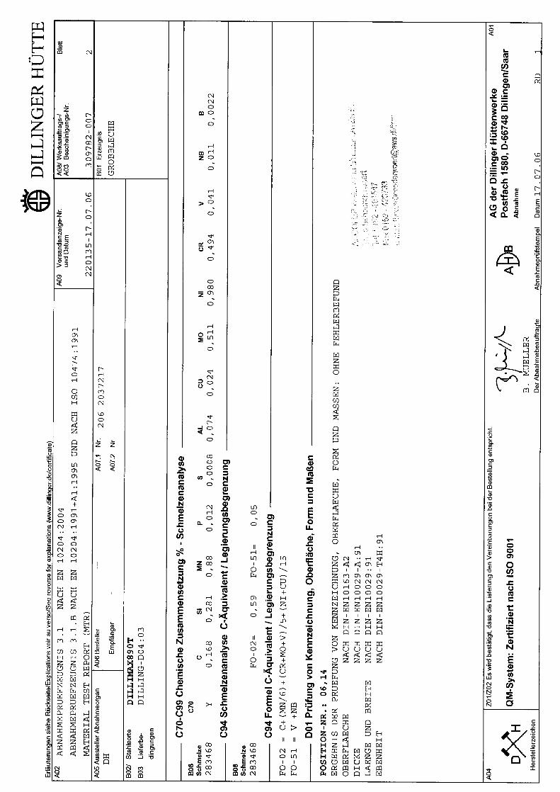


166

167
Annex E: Production data sheets TIG Dressing
On the following pages the production data sheets from the TIG‐dressing are displayed. Unfortunately some of the comments are in Dutch language.

PRODUCTION D A T A S H E E T f o r W E L D T O E I M P R O V E M E N T b y
TIG DRESSING
J f lPm; \ Internat ional Inst i tute of l ^ A p r - Welding ^= 3 =" ' C o m m i s s i o n XIII
WELDINp SPECIFICATION Base material: 3 rPtj O
Filler material:
Welding procedure No: C C? c\
COMPONENT
Type:
Identification: <! Cvh ^
EQUIPMENT Make and model: lA<duA p i P v
Power capacity: QS'oo fikv^ f
Electrode diameter: ^ y 2
Gas cup diameter: I 0 » A « V » .
Shieldina aas: A»R<££>tJ L.\ b
SKETCH OR PHOTO
TREATMENT DATA
Dressing position H G . 2G) etc: \ (z>
Preheat temperature: • OFr-> ° £1^
Gas flow rate: 11>~ —̂ /
Work angle, sideways: r*> O - o°
Work angle, weld direction: ( C\ c
Travel speed (S): /' Q.2- / T
V o l t a a e f V W p * - i% Current fl): 9 ^ ^ /
u 6 0 x S x / Heat input: n=
1 0 0 0 x 1 / (kJ/mm)
SKETCH OR PHOTO
/WSPEC7/OW • Visual jELPhoto • Geometry measurements
Equipment: L c A N ^ j C
REMARKS
TOE GEOMETRY MEASUREMENTS Spacing of measurement points (mm):
Max. Min. Mean
Toe radius (mm):
Groove depth (mm):
Measurements report:
REMARKS
OPERATOR
Experience: a). Hours: b). Length of weld treated: i ^ ^
Operator's name: • CA \Aa^^^T\ W-e'L.rA nota- S^(J^In b 111 1 uaie. —« ƒ '

PRODUCTION DATA S H E E T f o r W E L D T O E I M P R O V E M E N T by
TIG DRESSING
International Inst i tute of Welding
C o m m i s s i o n XIII
WELDING SPECIFICA TION Base material: d~». a
Filler material:
Welding procedure No:
COMPONENT
Type:
Identification: Z
EQUIPMENT Make and model: -è.^v^fiP^ SKETCH OR PHOTO
Power capacity: f - c y > JA-IAV,/"
Electrode diameter: _Ai 2.
Gas cup diameter: ^ ö i s / w ^
Shielding gas: Ê^üjJüX** (=\ 1 é
TREATMENT DATA
Dressing position (1G, 2G) etc:
Preheat temperature: O ° C -
Gas flow rate: l , r ^ -
Work angle, sideways: for> - °w a '•—'
Work angle, weld direction: ( Q
Travel speed (S): l?-2 ^ w - y
Voltage (V): . Current (I): ^ T ö A^-yj
Heat input: H=
(kJ/mm) 1 0 0 0 x #
INSPECTION • Visual • Photo • Geometry measurements
Equipment:
TOE GEOMETRY MEASUREMENTS Spacing of measurement points (mm): ,
REMARKS
x
-a l o o v A w ^ .
Max. Min. lean
Toe radius (mm):
Groove depth (mm):
leasurements report:
OPERATOR ? , b). Length of weld treated: OZL~L l,VVv<A Experience: a). Hours:
Operator's name: (^2i <£j Date

PRODUCTION DATA S H E E T f o r W E L D T O E I M P R O V E M E N T b y
TIG DRESSING
International Inst i tute of Weld ing
C o m m i s s i o n XIII
WELDING SPECIFICATION Base material: S 6
Filler material:
Welding procedure No: d " T ^ QJL<£ïh) rV>
EQUIPMENT Make and model: /^pt Power capacity: '2 C r ^ é j f ) fin p
Electrode diameter:
Gas cup diameter:
Shielding gas: /•) A c y w ^ ; /
TREATMENT DATA
Dressing position (1G, 2G) etc: < C
Preheat temperature: A ^ O
Gas flow rate: C zAh
Work angle, sideways:
Work angle, weld direction: jfi
O
Travel speed (S): j 0 1 / ^ . ^ / f/ua
Voltage (V): 0 - / £ ^ Current (I):' Artf
Heat input: H=
(kJ/mm)
6 0 x S x /
1 0 0 0 x 1 /
COMPONENT
Type:
Identification:
SKETCH OR PHOTO
INSPECTION • Visual • Photo • Geometry measurements
Equipment:
REMARKS
TOE GEOMETRY MEASUREMENTS Spacing of measurement points (mm):
Max. Min. Mean
Toe radius (mm): .
Groove depth (mm):
Measurements report:
Experience: a). Hours:
Operator's name: /
OPERATOR b). Length of weld treated: "b
Date: i l - 20 U

PRODUCTION DATA S H E E T f o r W E L D T O E I M P R O V E M E N T b y
TIG DRESSING
International Insti tute of Weld ing
C o m m i s s i o n XIII
WELDING SPECIFICATION Base material: _ƒ> //COCJ
Filler material:
Welding procedure No: i jf-; p i / ? / ° : > S " V ' ' ^
COMPONENT
Type: ,
Identification: ( 11
EQUIPMENT
Make and model: kx£j*££j. Power capacity: l^ïO* p
Electrode diameter:
Gas cup diameter: _
SKETCH OR PHOTO
y £2 <zi
Shielding gas: Afiy x-J 2 . . . d
TREATMENT DATA
Dressing position (1G, 2G) etc:
Preheat temperature:
Gas flow rate: IS I P/r>> I A/
A Q_ Work angle, sideways:
Work angle, weld direction: io
Travel speed (S)
Voltage (V): i}~ f< Current (I): <j£Ó Aw
Heat input: H=
(kJ/mm)
6 0 x 5 x 7 1 0 0 0 x 1 /
INSPECTION • Visual • Photo • Geometry measurements
Equipment: .
REMARKS
TOE GEOMETRY MEASUREMENTS Spacing of measurement points (mm):
5 ?
Max. l i n . Mean
Toe radius (mm):
Groove depth (mm): _
Measurements report:
OPERATOR b). Length of weld treated: 3,3>2 mm Experience: a). Hours:,
Operator's name: O - C$\Z/Xï*S 6t.ro Date: ).M •• / , - 96 jt
I

PRODUCTION DATA S H E E T f o r W E L D T O E I M P R O V E M E N T b y
TIG DRESSING
International Insti tute of Welding
C o m m i s s i o n XIII
WELDING SPECIFICATION Base material: & X cf<^>
Filler material:
Welding procedure No: / ij± d&£M
EQUIPMENT Make and model: /(kniPp><
Power capacity:_ 2 . ^ 0 7.1 A? /7l Electrode diameter:
Gas cup diameter: _
Shielding gas: AiiQa-AJ u-ó
TREATMENT DATA
Dressing position (1G, 2G) etc: ' C~
Preheat temperature: - / 2 -6 *_ c
Gas flow rate: /r> L I
Work angle, sideways: / o •• 0/D
Work angle, weld direction: / d
Travel speed (S): th^Cj T
Voltage (V): / ?, <l Current (I): Q^ó Ah f (
Heat input: H=
(kJ/mm)
6 0 x S x /
-\000xV
INSPECTION • Visual • Photo • Geometry measurements
Equipment:
TOÉ GEOMETRY MEASUREMENTS Spacing of measurement points (mm):
Max. l i n . Mean
Toe radius (mm): _
Groove depth (mm):.
leasurements report:
COMPONENT
Type:
Identification:
SKETCH OR PHOTO
REMARKS
/ \ f 2 i/o I C
A W«/ Ö / d t o ÖWÖ4S c/ f v^o o -2, **T7 ̂ <r«s^ ̂ A
Experience: a). Hours: OPERATOR
b). Length of weld treated: t j / j j
Operator's name: GJ ÈjDg. f^so.ès c?A C ^ Date

PRODUCTION DATA S H E E T f o r W E L D T O E I M P R O V E M E N T b y
TIG DRESSING
|\. International Inst i tute of Welding
C o m m i s s i o n XIII
WELDING SPECIFICATION Base material: ö> Ó. E^fg
/ Filler material:
Welding procedure No:
EQUIPMENT Make and model: A / f / r V P p '
Power capacity: 1 -S'o P
2 Electrode diameter: _ _
Gas cup diameter: /£> /n
Shielding gas: $L0J± ON
TREATMENT DATA
Dressing position (1G, 2G) etc: > &
Preheat temperature: • / O O c
Gas flow rate:
Work angle, sideways:
Work angle, weld direction: /é>
Travel speed (S): m
Voltage (V): /Jh / 7
~ / S Current (I): O ^ O
Heat input: H=
(kJ/mm)
6 0 x S x /
1 0 0 0 x V
COMPONENT
Type:
Identification: Ï7Z
SKETCH OR PHOTO
INSPECTION • Visual • Photo • Geometry measurements
Equipment:
TOE GEOMETRY MEASUREMENTS Spacing of measurement points (mm):
REMARKS .
/ O O C C
Max. Iin. Mean
Toe radius (mm):
Groove depth (mm):
Measurements report:
OPERATOR Experience: a). Hours: b). Length of weld treated: 3>3p tt^/f Operator's name: (g^ó/t^l &•- -3- Date : 3Ö 2&LL

PRODUCTION DATA S H E E T f o r W E L D T O E I M P R O V E M E N T b y
TIG DRESSING
International Inst i tute of •ÏM^M Welding
" • C o m m i s s i o n XIII
WELDING SPECIFICATION Base material: Q ^ f ó C J
Filler material:
Weldinq procedure No: " T ^ n t a o ^ s l »v«2»
COMPONENT
Type:
Identification: V A* ó
EQUIPMENT Make and model: idiS/npp' ci.^Oci W
i I Power capacity: ' 2 ^ o j@sn^
Electrode diameter: r*> /*v
Gas cup diameter: JO t*1 ^
Shieldina aas: A/Z4,a>sS / { ^
SKETCH OR PHOTO
TREATMENT DATA
Dressina position (1G. 2G) etc: ' d
Preheat temperature: • DO <¬
Gas flow rate: /vT Z f /r*.t,\>
Work anqle. sideways: />o -
Work angle, weld direction: ' Ö
Travel speed (S): f 'jH* I
V o I t a a e M : / 3 - / c ? Current (I): 2 b ö / V J ?
, . 6 0 x S x / Heat input: n = =
1 0 0 0 x 1 / (kJ/mm)
SKETCH OR PHOTO
INSPECTION • Visual • Photo • Geometry measurements
Equipment:
REMARKS ,
/QO / ? <r> p
1 3 - / / , V
TOE GEOMETRY MEASUREMENTS Spacing of measurement points (mm):
Max. Min. Mean
Toe radius (mm):
Groove depth (mm):
Measurements report:
REMARKS ,
/QO / ? <r> p
1 3 - / / , V
OPERATOR Experience: a). Hours: b). Length of weld treated: 3QV'j /"/*•
Date: 3 ^ I g g ' /

PRODUCTION DATA S H E E T f o r W E L D T O E I M P R O V E M E N T b y
TIG DRESSING
/{jifjwlfc, International Inst i tute of Welding
C o m m i s s i o n XIII
WELDING SPECIFICATION
Base material: - 8><a CJ
Filler material:
Welding procedure No:
COMPONENT
Tvoe:
Identification: ^ /
EQUIPMENT Make and model: /Q-mpdi "2A'oo \rJ
J r\ Power capacity: 9 < C> A /ft \v
Electrode diameter: 3 . % /w m
Gas cup diameter: /O m PI.
Shieldinq aas: A ilo^iu -6
SKETCH OR PHOTO
TREATMENT DATA
Dressing position (1G. 2G) etc: / ó
Preheat temperature: • /'IS ~c
Gas flow rate: / / */mx/\j
Work anale, sideways: &t> - Qo '
Work anqle, weld direction: id
Travel speed (S): j'70 n /* t
Voltaae (V): / } - /&, Current (I): 2<<o p u .. . JeoxSxi Heat input: H= =
1 0 0 0 x 1 / (kJ/mm)
SKETCH OR PHOTO
INSPECTION • Visual • Photo . • Geometry measurements
Equipment:
REMARKS
2 A p TOE GEOMETRY MEASUREMENTS
Spacing of measurement points (mm):
Max. Min. Mean
Toe radius (mm):
Groove depth (mm):
Measurements report:
REMARKS
2 A p
OPERATOR
Experience: a). Hours: b). Length of weld treated: 3 2 3 <*IV1
Operator's name: . QQC>£JO&'V h£A<H Date: A O - ^ • 2ö ^

5
PRODUCTION DATA S H E E T f o r W E L D T O E I M P R O V E M E N T b y
TIG DRESSING
International Inst i tute of Welding
C o m m i s s i o n XIII
WELDING SPECIFICATION Base material: S l/£lQ> Filler material:
Welding procedure No: 1
4 r
EQUIPMENT Make and model: /L/k'^vPpi 9 , ^ o d ^
Power capacity:
Electrode diameter:
Gas cup diameter:.
Shielding gas: Hgc^ ^ . d
/ O / V ) / O - .
J
TREATMENT DATA
Dressing position (1G, 2G) etc: 1 £•
Preheat temperature: / Qr5> _
Gas flow rate: /-"•> / /, I r
Work angle, sideways: - 9s
Work angle, weld direction: /a d
<3_
Travel speed (S):
Voltage (V): / ? - / | Current (I): 2 S£j
Heat input: /-/=
(kJ/mm)
6 0 x 5 x /
1 0 0 0 x V
COMPONENT
Type:
Identification: 1 / / (
SKETCH OR PHOTO
INSPECTION • Visual • Photo • Geometry measurements
Equipment:
REMARKS
TOE GEOMETRY MEASUREMENTS Spacing of measurement points (mm):
Max. lin. lean
Toe radius (mm): _
Groove depth (mm):.
Measurements report:
Experience: a). Hours:. OPERATOR
b). Length of weld treated: 323 ^INR>
Operator's name: t
Date: ?G I I

177
Annex F: Matlab scripts to process weld geometry data
Splitting of laser position and measured data and subtracting a plane.
%split A in X, Y en Z values gr=size(A); rijen_m=gr(1,1); kolommen_n=gr(1,2); Xs=A(1,:); X=Xs(1,2:kolommen_n(1,1)); %create vector containing x-values Ys=A(:,1); Y=Ys(2:rijen_m(1,1),1); %create vector containing y-values Zster=A(2:rijen_m(1,1),2:kolommen_n(1,1)); %extract Z values %Construct a plane to level the weld cross sections at 0 x1=0; %first point to equal to zero y1=7; z1=1.4481; x2=53; %second point to equal to zero y2=7; z2=0.1411; x3=0; %third point to equal to zero y3=140; z3=0.7353; gridsizex=0.01; %define grid size of data gridsizey=7; F=[x1 y1 1; x2 y2 1; x3 y3 1]; v=[z1; z2; z3]; abc=F\v; VLAK=zeros(rijen_m(1,1)-1,kolommen_n(1,1)-1); for n=1:(kolommen_n(1,1)-1) for m=1:(rijen_m(1,1)-1) xwaarde=X(1,n); ywaarde=Y(m,1); VLAK(m,n)=abc(1,1)*xwaarde+abc(2,1)*ywaarde+abc(3,1); end; end; %Substract created plane from Z values Z=(Zster-VLAK)*-1; %Plot Weld surf(X,Y,Z,'LineWidth',0.1,'Linestyle','-') %create 3D plot title('Weld geometry'), xlabel('Dimension across the weld'), ylabel('Dimension along the weld'), axis equal; clear Xs Ys Zster x1 y1 x2 y2 x3 y3 z1 z2 z3 xwaarde ywaarde VLAK gr m n abc F v;

178
Determining the weld toe radius
%define optimalisation boundaries ondergrens=46; %lower boundary, use steps of size: [gridsizex] bovengrens=47; %upper boundary, use steps of size: [gridsizex] apphmid=2; %estimate of height of circle midpoint6 hoogtegrid=2.5; %height of grid in mm breedtegrid=2.5; %width of grid in mm gridstap=0.025; %grid spacing %building of the grid lgrid=breedtegrid/gridstap+1; hgrid=hoogtegrid/gridstap+1; hcoor=zeros(1,lgrid); vcoor=zeros(hgrid,1); for k=1:lgrid hcoor(1,k)=(bovengrens+ondergrens)/2-breedtegrid/2+(k-1)*gridstap; end for l=1:hgrid vcoor(l,1)=apphmid+hoogtegrid/2-(l-1)*gridstap; end %build two vectors to show the grid vectorgridplothor=hcoor; m=1; while m<hgrid; vectorgridplothor=[vectorgridplothor hcoor]; m=m+1; end vectorgridplotver=vcoor(1,1)*ones(1,lgrid); mm=2; while mm<hgrid+1; hulpvector=vcoor(mm,1)*ones(1,lgrid); vectorgridplotver=[vectorgridplotver hulpvector]; mm=mm+1; end scatter(vectorgridplothor,vectorgridplotver,'.g') axis equal hold on; %for all gridpoints, calculate distance to all data points within %optimalisation boundaries, determine average distance and deviation Mafw=zeros(hgrid,lgrid); Mstr=zeros(hgrid,lgrid); vanscancol=round(ondergrens/gridsizex+1); totscancol=round(bovengrens/gridsizex+1); scanpointsx=X(1,vanscancol:totscancol); scanpointsy=Z(rij,vanscancol:totscancol); grscptx=size(scanpointsx); afst=zeros(grscptx(1,2),1); for q=1:hgrid for r=1:lgrid for t=1:grscptx(1,2) afst(t,1)=sqrt((hcoor(1,r)-scanpointsx(1,t))^2+(vcoor(q,1)-scanpointsy(1,t))^2); end

179
gem=mean(afst); vgem=gem*ones(grscptx(1,2),1); afw=afst-vgem; Mstr(q,r)=gem; Mafw(q,r)=sum(abs(afw)); end end %find minimum value in matrix Mr [minpercol,rijentry]=min(Mafw); [mintot,colentry]=min(minpercol); entryrijcol=[rijentry(1,colentry) colentry]; %find calculated optimum radius and midpoint coordinates ropt=Mstr(entryrijcol(1,1),entryrijcol(1,2)); afwijkingvangem=Mafw(entryrijcol(1,1),entryrijcol(1,2)); xopt=hcoor(1,entryrijcol(1,2)); yopt=vcoor(entryrijcol(1,1),1); %draw optimum midpoint scatter(xopt,yopt,'or'); %draw circle for tel=1:1000 cirkelx(tel)=ropt*cos(tel/100)+xopt; cirkely(tel)=ropt*sin(tel/100)+yopt; end plot(cirkelx, cirkely); clear cirkelx cirkely grscptx afst afw vgem Mstr Mafw minpercol rijentry colentry afwijkingvangem; clear ondergrens bovengrens apphmid hoogtegrid breedtegrid gridstap lgrid hgrid hcoor vcoor; clear k l vectorgridplothor vectorgridplotver mintot entryrijcol afwijkingvangem tel;
Determining the weld toe angle
%determine weld toe angle vanmoe=44; %start of straight parent material, use steps of size [gridsizex] totmoe=45; %end of straight parent material, use steps of size [gridsizex] vanlas=50; %start of straight weld material, use steps of size [gridsizex] totlas=52; %end of straight weld material, use steps of size [gridsizex] vanhoekmoecol=round(vanmoe/gridsizex+1); tothoekmoecol=round(totmoe/gridsizex+1); vanhoeklascol=round(vanlas/gridsizex+1); tothoeklascol=round(totlas/gridsizex+1); Xmoepoints=X(1,vanhoekmoecol:tothoekmoecol); Zmoepoints=Z(rij,vanhoekmoecol:tothoekmoecol); Xlaspoints=X(1,vanhoeklascol:tothoeklascol); Zlaspoints=Z(rij,vanhoeklascol:tothoeklascol); moe=polyfit(Xmoepoints,Zmoepoints,1); las=polyfit(Xlaspoints,Zlaspoints,1); %plot of both fitted lines
180
xmoe=vanmoe:gridsizex:totmoe; zmoe=moe(1)*xmoe+moe(2); plot(xmoe,zmoe) hold on; xlas=vanlas:gridsizex:totlas; zlas=las(1)*xlas+las(2); plot(xlas,zlas); hoekmoe=atand(moe(1)); %angle of parent material with horizontal hoeklas=atand(las(1)); %angle of weld material with horizontal hoekverschil=abs(hoeklas-hoekmoe); %angle between parent material and weld clear vanhoekmoecol tothoekmoecol vanhoeklascol tothoeklascol Xmoepoints Xlaspoints Zlaspoints moe las xmoe zmoe xlas zlas hoekmoe hoeklas;
Determining the weld height
%determine undercut of weld in relation to parent material left=3.; %left location of parent material, use steps of size [gridsizex] right=50; %right location parent material, use steps of size [gridsizex] vanh=5; %start of area under investigation for weld height use septs of size [gridsizex] toth=52; %end of area under investigation for weld height use steps of size [gridsizex] %construct refenence line leftcol=round(left/gridsizex+1); rightcol=round(right/gridsizex+1); leftz=Z(rij,leftcol); rightz=Z(rij,rightcol); xline=[left right]; zline=[leftz rightz]; parent=polyfit(xline,zline,1); plot(xline,zline); %determine distance of weld to reference line vanhcol=round(vanh/gridsizex+1); tothcol=round(toth/gridsizex+1); scanpointsx=X(1,vanhcol:tothcol); scanpointsz=Z(rij,vanhcol:tothcol); grscptx=size(scanpointsx); Dist=zeros(1,grscptx(1,2)); for dtel=1:grscptx(1,2); Dist(1,dtel)=scanpointsz(1,dtel)-(parent(1,1)*scanpointsx(1,dtel)+parent(1,2)); end weldheight=max(Dist); clear left right vanh toth leftcol rightcol leftz rightz xline zline parent; clear scanpointsx scanpointsz vanhcol tothcol grscptx Dist;
Determining the undercut
%determine undercut of weld in relation to parent material vanmoe=48; %start of straight parent material, use steps of size [gridsizex] totmoe=49; %end of straight parent material, use steps of size [gridsizex]

181
vancut=47; %start of area under investigation for undercut use steps of size [gridsizex] totcut=51; %end of area under investigation for undercut use steps of size [gridsizex] vancutmoecol=round(vanmoe/gridsizex+1); totcutmoecol=round(totmoe/gridsizex+1); vancutweldcol=round(vancut/gridsizex+1); totcutweldcol=round(totcut/gridsizex+1); Xmoepoints=X(1,vancutmoecol:totcutmoecol); Zmoepoints=Z(rij,vancutmoecol:totcutmoecol); moe=polyfit(Xmoepoints,Zmoepoints,1); scanpointsx=X(1,vancutweldcol:totcutweldcol); grscptx=size(scanpointsx); scanpointsz=Z(rij,vancutweldcol:totcutweldcol); reflijnx=X(1,vancutweldcol:totcutweldcol); for reftel=1:grscptx(1,2) reflijnz(1,reftel)=moe(1)*scanpointsx(1,reftel)+moe(2); end plot(scanpointsx,reflijnz); Dist=zeros(1,grscptx(1,2)); for dtel=1:grscptx(1,2) Dist(1,dtel)=reflijnz(1,dtel)-scanpointsz(1,dtel); end undercut=max(Dist); clear vanmoe tot moe vancut totcut vancutmoecol totcutmoecol vancutweldcol; clear totcutweldcol Xmoepoints Zmoepoints moe scanpointsx grscptx; clear scanpointsz reflijnx reftel reflijnz Dist dtel;

182

183
Annex G: Collaboration with TNO: Acoustic emission
In this research the location of cracks and crack initiation time have been determined with the aid of strain gauges. Another possibility is the use of the acoustic emission of the steel when a crack is growing. To detect these sound emissions of the steel, sensors have been applied on a number of specimens. To reduce background noise from the hydraulics of the testing rig, plasticine dampers have been applied. The resulting test setup can be seen in figure G.1.
figure G.1 Left: test setup with sensors and dampers applied to the specimen. Right: close up of three sensors without any cables attached and two dampers made of plasticine, pretensioned with bicycle tires.
Due to the nature of the testing rig a very high background noise level was measured. This can be damped by the dampers as depicted in figure G.1 or by placing insulating material between the clamps of the test rig. Because the considered rig is an axial test rig which uses clamping to fix the specimens, the second option for background noise reduction was not possible. The dampers are able to reduce the background noise to a certain extent, but not always to the desired level, depending on the thickness of the specimen and the magnitude of the applied load and frequency. The sensors are able to locate a crack via triangulation of the signal at different sensors. The software then produces a
summation of all ‘hits’ which results in an image as can be seen in figure G.2. This location of the crack can only be done in a rather coarse manner because of the relatively large size of the sensors in relation to the weld. In practice, larger structures will be observed and smaller sensors are available.
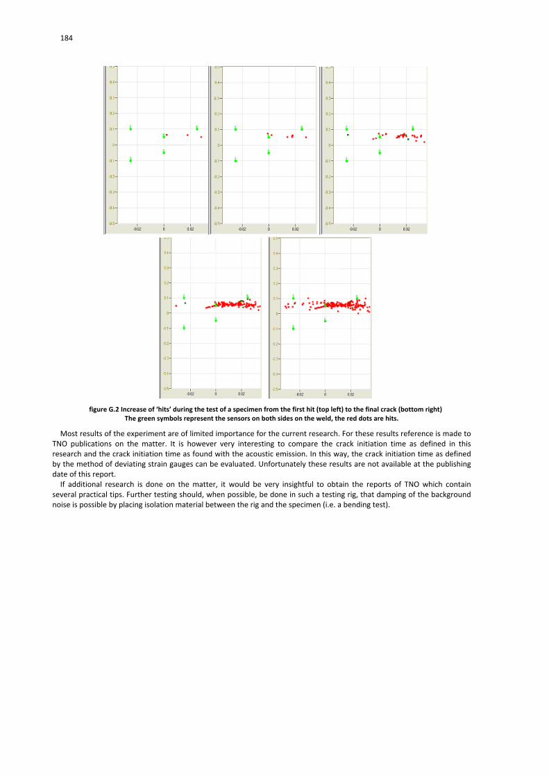
184
figure G.2 Increase of ‘hits’ during the test of a specimen from the first hit (top left) to the final crack (bottom right) The green symbols represent the sensors on both sides on the weld, the red dots are hits.
Most results of the experiment are of limited importance for the current research. For these results reference is made to TNO publications on the matter. It is however very interesting to compare the crack initiation time as defined in this research and the crack initiation time as found with the acoustic emission. In this way, the crack initiation time as defined by the method of deviating strain gauges can be evaluated. Unfortunately these results are not available at the publishing date of this report. If additional research is done on the matter, it would be very insightful to obtain the reports of TNO which contain
several practical tips. Further testing should, when possible, be done in such a testing rig, that damping of the background noise is possible by placing isolation material between the rig and the specimen (i.e. a bending test).

185
Annex H: Hardness Measurements
From each plate material one strip of residual material has been polished. Pijpers (2011) has shown on similar specimens from the same material that the hardness does not vary significantly over the height of the specimen, but only shows differences between the different material states (fusion zone FZ, heat affected zone HAZ and base material BM). From each specimen the as welded situation is plotted. All measurements are executed after TIG‐dressing, but only in the middle of the specimen, which is assumed to be out of the influence of TIG‐dressing. Then, the comparison with the effect of TIG dressing is made. The different zones that occur after the initial welding
process (FZ, HAZ and BM) can each separately be influenced by the TIG dressing, by being remelted or heat affected. In the diagrams the different zones that occur after initial welding are stated as the ‘as welded’ situation, and the effects of TIG‐dressing (melting of heat affecting) on these original zones are plotted for comparison. For example: figure H.4 shows datapoints which were in the BM zone after welding. Some areas of the BM zone have been influenced by TIG dressing, denoted by TIG Fluid Zone and TIG Heat Affected Zone. These points are plotted in white and grey. Because of the complex geometry of the different zones after TIG‐dressing, the X‐axis in these comparison diagrams has no meaning, the diagram is simply a comparison of different measured values. An example of the as welded state of a specimen is shown in figure H.1. The effect of TIG‐dressing is shown in figure H.2.
Note that in figure H.2 the fluid zone of TIG‐dressing at the cap side of the weld extends into the as welded FZ, HAZ and BM. This is in reality not always the case. Similar remarks can be made at the other fluid zones and heat affected zones.
FZ HAZHAZBM BM
figure H.1 Zones in the as welded specimens
figure H.2 Effect of TIG‐dressing
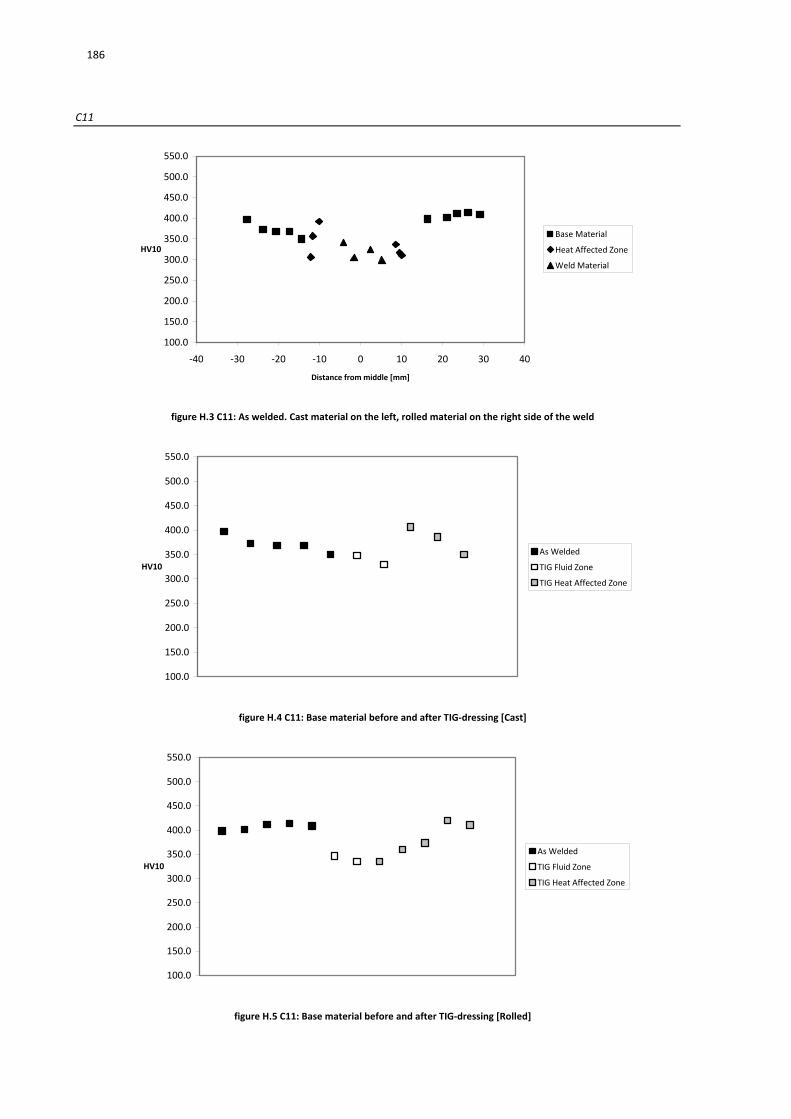
186
C11
100.0
150.0
200.0
250.0
300.0
350.0
400.0
450.0
500.0
550.0
‐40 ‐30 ‐20 ‐10 0 10 20 30 40
Distance from middle [mm]
HV10
Base Material
Heat Affected Zone
Weld Material
figure H.3 C11: As welded. Cast material on the left, rolled material on the right side of the weld
100.0
150.0
200.0
250.0
300.0
350.0
400.0
450.0
500.0
550.0
HV10
As Welded
TIG Fluid Zone
TIG Heat Affected Zone
figure H.4 C11: Base material before and after TIG‐dressing [Cast]
100.0
150.0
200.0
250.0
300.0
350.0
400.0
450.0
500.0
550.0
HV10
As Welded
TIG Fluid Zone
TIG Heat Affected Zone
figure H.5 C11: Base material before and after TIG‐dressing [Rolled]

187
100.0
150.0
200.0
250.0
300.0
350.0
400.0
450.0
500.0
550.0
HV10
As Welded
TIG Fluid Zone
TIG Heat Affected Zone
figure H.6 C11: Heat affected zone before and after TIG‐dressing [Cast]
100.0
150.0
200.0
250.0
300.0
350.0
400.0
450.0
500.0
550.0
HV10
As Welded
TIG Fluid Zone
TIG Heat Affected Zone
figure H.7 C11: Heat affected zone before and after TIG‐dressing [Rolled]
100.0
150.0
200.0
250.0
300.0
350.0
400.0
450.0
500.0
550.0
HV10
As Welded
TIG Fluid Zone
TIG Heat Affected Zone
figure H.8 C11: Fluid zone before and after TIG‐dressing

188
C89
100.0
150.0
200.0
250.0
300.0
350.0
400.0
450.0
500.0
550.0
‐40 ‐30 ‐20 ‐10 0 10 20 30 40
Distance from middle [mm]
HV10
Base Material
Heat Affected Zone
Weld Material
figure H.9 C89: As welded. Cast material on the left, rolled material on the right side of the weld
100.0
150.0
200.0
250.0
300.0
350.0
400.0
450.0
500.0
550.0
HV10
As Welded
TIG Fluid Zone
TIG Heat Affected Zone
figure H.10 C89: Base material before and after TIG‐dressing [Cast]
100.0
150.0
200.0
250.0
300.0
350.0
400.0
450.0
500.0
550.0
HV10
As Welded
TIG Fluid Zone
TIG Heat Affected Zone
figure H.11 C89: Base material before and after TIG‐dressing [Rolled]

189
100.0
150.0
200.0
250.0
300.0
350.0
400.0
450.0
500.0
550.0
HV10
As Welded
TIG Fluid Zone
TIG Heat Affected Zone
figure H.12 C89: Heat affected zone before and after TIG‐dressing [Cast]
100.0
150.0
200.0
250.0
300.0
350.0
400.0
450.0
500.0
550.0
HV10
As Welded
TIG Fluid Zone
TIG Heat Affected Zone
figure H.13 C89: Heat affected zone before and after TIG‐dressing [Rolled]
100.0
150.0
200.0
250.0
300.0
350.0
400.0
450.0
500.0
550.0
HV10
As Welded
TIG Fluid Zone
TIG Heat Affected Zone
figure H.14 C89: Fluid zone before and after TIG‐dressing
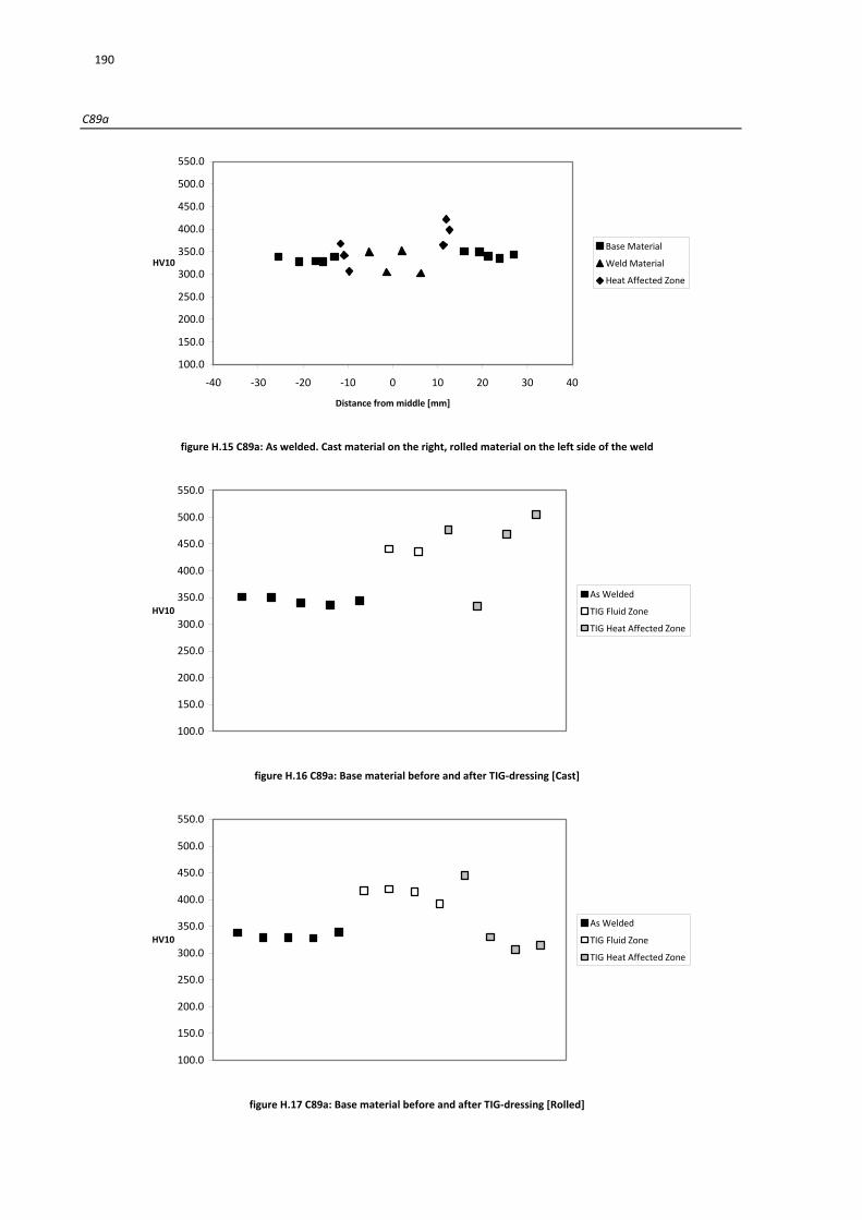
190
C89a
100.0
150.0
200.0
250.0
300.0
350.0
400.0
450.0
500.0
550.0
‐40 ‐30 ‐20 ‐10 0 10 20 30 40
Distance from middle [mm]
HV10
Base Material
Weld Material
Heat Affected Zone
figure H.15 C89a: As welded. Cast material on the right, rolled material on the left side of the weld
100.0
150.0
200.0
250.0
300.0
350.0
400.0
450.0
500.0
550.0
HV10
As Welded
TIG Fluid Zone
TIG Heat Affected Zone
figure H.16 C89a: Base material before and after TIG‐dressing [Cast]
100.0
150.0
200.0
250.0
300.0
350.0
400.0
450.0
500.0
550.0
HV10
As Welded
TIG Fluid Zone
TIG Heat Affected Zone
figure H.17 C89a: Base material before and after TIG‐dressing [Rolled]

191
100.0
150.0
200.0
250.0
300.0
350.0
400.0
450.0
500.0
550.0
HV10
As Welded
TIG Fluid Zone
TIG Heat Affected Zone
figure H.18 C89a: Heat affected zone before and after TIG‐dressing [Cast]
100.0
150.0
200.0
250.0
300.0
350.0
400.0
450.0
500.0
550.0
HV10
As Welded
TIG Fluid Zone [no data]
TIG Heat Affected Zone
figure H.19 C89a: Heat affected zone before and after TIG‐dressing [Rolled]
100.0
150.0
200.0
250.0
300.0
350.0
400.0
450.0
500.0
550.0
HV10
As Welded
TIG Fluid Zone
TIG Heat Affected Zone
figure H.20 C89a: Fluid zone before and after TIG‐dressing

192
C69
100.0
150.0
200.0
250.0
300.0
350.0
400.0
450.0
500.0
550.0
‐40 ‐30 ‐20 ‐10 0 10 20 30 40
Distance from middle [mm]
HV10
Base Material
Heat Affected Zone
Weld Material
figure H.21 C69: As welded. Cast material on the right, rolled material on the left side of the weld
100.0
150.0
200.0
250.0
300.0
350.0
400.0
450.0
500.0
550.0
HV10
As Welded
TIG Fluid Zone
TIG Heat Affected Zone
figure H.22 C69: Base material before and after TIG‐dressing [Cast]
100.0
150.0
200.0
250.0
300.0
350.0
400.0
450.0
500.0
550.0
HV10
As Welded
TIG Fluid Zone
TIG Heat Affected Zone
figure H.23 C69: Base material before and after TIG‐dressing [Rolled]

193
100.0
150.0
200.0
250.0
300.0
350.0
400.0
450.0
500.0
550.0
HV10
As Welded
TIG Fluid Zone
TIG Heat Affected Zone
figure H.24 C69: Heat affected zone before and after TIG‐dressing [Cast]
100.0
150.0
200.0
250.0
300.0
350.0
400.0
450.0
500.0
550.0
HV10
As Welded
TIG Fluid Zone
TIG Heat Affected Zone
figure H.25 C69: Heat affected zone before and after TIG‐dressing [Rolled]
100.0
150.0
200.0
250.0
300.0
350.0
400.0
450.0
500.0
550.0
HV10
As Welded
TIG Fluid Zone
TIG Heat Affected Zone
figure H.26 C69: Fluid zone before and after TIG‐dressing

194
C46
100.0
150.0
200.0
250.0
300.0
350.0
400.0
450.0
500.0
550.0
‐40 ‐30 ‐20 ‐10 0 10 20 30 40
Distance from middle [mm]
HV10
Base Material
Heat Affected Zone
Weld Material
figure H.27 C46: As welded Cast material on the right, rolled material on the left side of the weld
100.0
150.0
200.0
250.0
300.0
350.0
400.0
450.0
500.0
550.0
HV10
As Welded
TIG Fluid Zone
TIG Heat Affected Zone
figure H.28 C46: Base material before and after TIG‐dressing [Cast]
100.0
150.0
200.0
250.0
300.0
350.0
400.0
450.0
500.0
550.0
HV10
As Welded
TIG Fluid Zone
TIG Heat Affected Zone
figure H.29 C46: Base material before and after TIG‐dressing [Rolled]
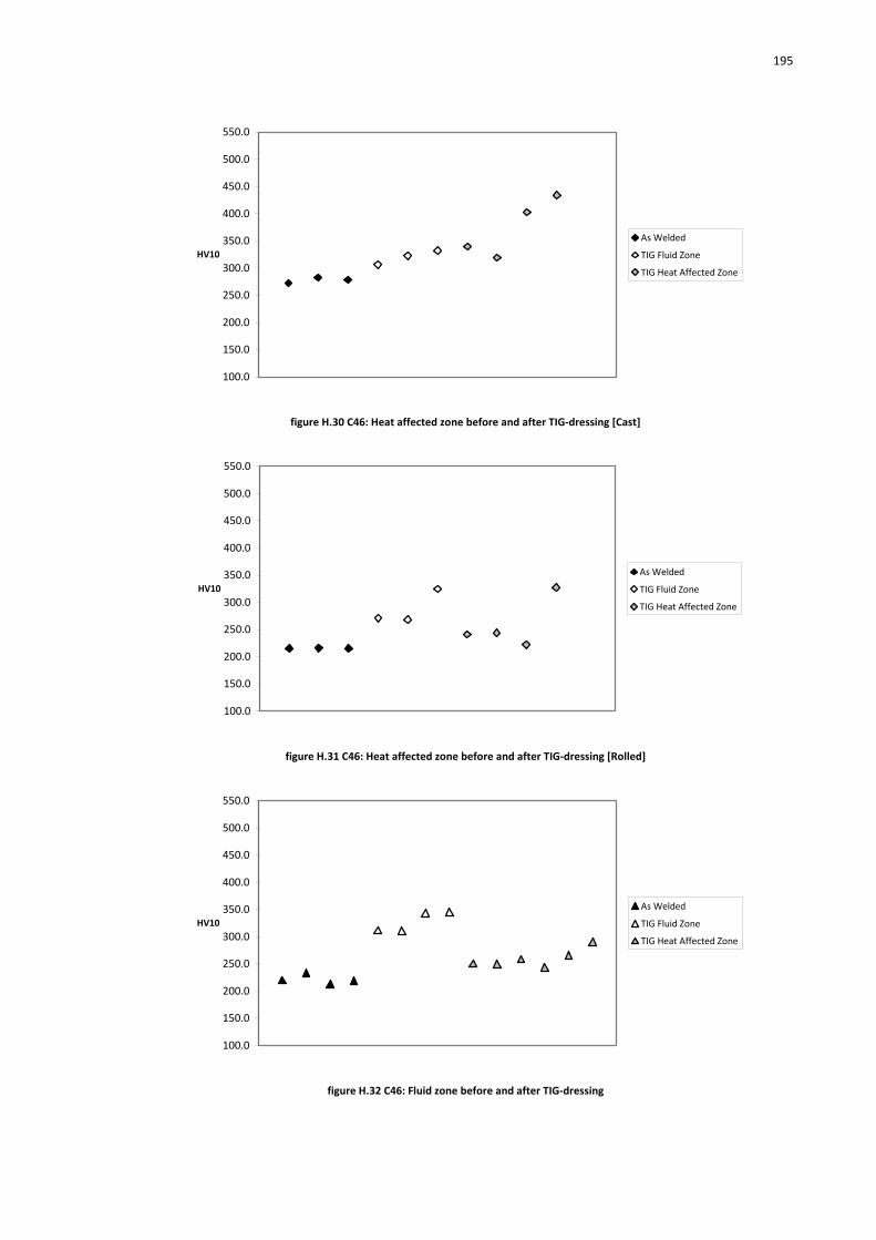
195
100.0
150.0
200.0
250.0
300.0
350.0
400.0
450.0
500.0
550.0
HV10
As Welded
TIG Fluid Zone
TIG Heat Affected Zone
figure H.30 C46: Heat affected zone before and after TIG‐dressing [Cast]
100.0
150.0
200.0
250.0
300.0
350.0
400.0
450.0
500.0
550.0
HV10
As Welded
TIG Fluid Zone
TIG Heat Affected Zone
figure H.31 C46: Heat affected zone before and after TIG‐dressing [Rolled]
100.0
150.0
200.0
250.0
300.0
350.0
400.0
450.0
500.0
550.0
HV10
As Welded
TIG Fluid Zone
TIG Heat Affected Zone
figure H.32 C46: Fluid zone before and after TIG‐dressing

196
V11
100.0
150.0
200.0
250.0
300.0
350.0
400.0
450.0
500.0
550.0
‐30 ‐20 ‐10 0 10 20 30 40
Distance from middle [mm]
HV10
Base Material
Heat Affected Zone
Weld Material
figure H.33 V11: As welded
100.0
150.0
200.0
250.0
300.0
350.0
400.0
450.0
500.0
550.0
HV10
As Welded
TIG Fluid Zone [no data]
TIG Heat Affected Zone
figure H.34 V11: Base material before and after TIG‐dressing
100.0
150.0
200.0
250.0
300.0
350.0
400.0
450.0
500.0
550.0
HV10
As Welded
TIG Fluid Zone
TIG Heat Affected Zone
figure H.35 V11:Heat affected zone before and after TIG‐dressing

197
100.0
150.0
200.0
250.0
300.0
350.0
400.0
450.0
500.0
550.0
HV10
As Welded
TIG Fluid Zone
TIG Heat Affected Zone
figure H.36 V11: Fluid zone before and after TIG‐dressing

198
V89
100.0
150.0
200.0
250.0
300.0
350.0
400.0
450.0
500.0
550.0
‐40 ‐30 ‐20 ‐10 0 10 20 30 40
Distance from middle [mm]
HV10
Base Material
Heat Affected Zone
Weld Material
figure H.37 V89: As welded
100.0
150.0
200.0
250.0
300.0
350.0
400.0
450.0
500.0
550.0
HV10
As Welded
TIG Fluid Zone
TIG Heat Affected Zone
figure H.38 V89: Base material before and after TIG‐dressing
100.0
150.0
200.0
250.0
300.0
350.0
400.0
450.0
500.0
550.0
HV10
As Welded
TIG Fluid Zone
TIG Heat Affected Zone
figure H.39 V89: Heat affected zone before and after TIG‐dressing

199
100.0
150.0
200.0
250.0
300.0
350.0
400.0
450.0
500.0
550.0
HV10
As Welded
TIG Fluid Zone
TIG Heat Affected Zone
figure H 40 V89: Fluid zone before and after TIG‐dressing

200
V69
100.0
150.0
200.0
250.0
300.0
350.0
400.0
450.0
500.0
550.0
-40 -30 -20 -10 0 10 20 30 40
Distance from middle [mm]
HV10
Base Material
Heat Affected Zone
Weld Material
figure H.41 V69: As welded
100.0
150.0
200.0
250.0
300.0
350.0
400.0
450.0
500.0
550.0
HV10
As Welded
TIG Fluid Zone
TIG Heat Affected Zone
figure H.42 V69: Base material before and after TIG0‐dressing
100.0
150.0
200.0
250.0
300.0
350.0
400.0
450.0
500.0
550.0
HV10
As Welded
TIG Fluid Zone
TIG Heat Affected Zone
figure H.43 V69: Heat affected zone before and after TIG‐dressing

201
100.0
150.0
200.0
250.0
300.0
350.0
400.0
450.0
500.0
550.0
HV10
As Welded
TIG Fluid Zone
TIG Heat Affected Zone
figure H.44 V69: Fluid zone before and after TIG‐dressing

202
V46
100.0
150.0
200.0
250.0
300.0
350.0
400.0
450.0
500.0
550.0
‐40 ‐30 ‐20 ‐10 0 10 20 30 40
Distance from middle [mm]
HV10
Base Material
Heat Affected Zone
Weld Material
figure H.45 V46: As welded
100.0
150.0
200.0
250.0
300.0
350.0
400.0
450.0
500.0
550.0
HV10
As Welded
TIG Fluid Zone
TIG Heat Affected Zone
figure H.46 V46: Base material before and after TIG‐dressing
100.0
150.0
200.0
250.0
300.0
350.0
400.0
450.0
500.0
550.0
HV10
As Welded
TIG Fluid Zone
TIG Heat Affected Zone
figure H.47 V46: Heat affected zone before and after TIG‐dressing

203
100.0
150.0
200.0
250.0
300.0
350.0
400.0
450.0
500.0
550.0
HV10
As Welded
TIG Fluid Zone
TIG Heat Affected Zone
figure H.48 V46: Fluid zone before and after TIG‐dressing

204

205
Annex I: Crack monitoring results
In the following diagrams the results of the crack monitoring are plotted. All values are given in the crack dimensions a and c. For edge cracks this is equal to the length and diameter of the crack, for surface cracks the actual crack width is 2∙c Only the specimens which have shown usable results are plotted. Note that the crack depth a measured from surface
measurements can differ from the crack marking measurements because the depth of the crack at the side is not necessarily the same as the maximum depth anywhere in the cross section. In case of a rerun specimen, only the second test is considered.
0.0
5.0
10.0
15.0
20.0
25.0
30.0
35.0
1.00E+06 1.02E+06 1.04E+06 1.06E+06 1.08E+06 1.10E+06
N
a/c [mm]
Crack width c
Crack depth a
Crack width c [CM]
Crack depth a [CM]
figure I.1 Crack propagation data of specimen C11‐2
0.0
2.0
4.0
6.0
8.0
10.0
6.00E+04 7.00E+04 8.00E+04 9.00E+04 1.00E+05 1.10E+05
N
a/c [mm]
Crack width c
Crack depth a
Crack width c [CM]
Crack depth a [CM]
figure I.2 Crack propagation data of specimen C89‐2

206
0.0
10.0
20.0
30.0
40.0
50.0
60.0
7.00E+04 8.00E+04 9.00E+04 1.00E+05 1.10E+05
N
a/c [mm]
Crack width c
Crack depth a
Crack width c [CM]
Crack depth a [CM]
figure I.3 Crack propagation data of specimen C89a‐1
0.0
10.0
20.0
30.0
40.0
1.00E+05 1.10E+05 1.20E+05 1.30E+05 1.40E+05 1.50E+05 1.60E+05
N
a/c [mm]
Crack width c
Crack depth a
Crack width c [CM]
Crack depth a [CM]
figure I.4 Crack propagation data of specimen C69‐1
0.0
5.0
10.0
15.0
20.0
25.0
30.0
5.40E+05 5.80E+05 6.20E+05 6.60E+05 7.00E+05
N
a/c [mm]
Crack width c
Crack depth a
Crack width c [CM]
Crack depth a [CM]
figure I 5 Crack propagation data of specimen C69‐2

207
0.0
5.0
10.0
15.0
20.0
25.0
30.0
3.10E+06 3.12E+06 3.14E+06 3.16E+06 3.18E+06 3.20E+06
N
a/c [mm]
Crack width c
Crack depth a
Crack width c [CM]
Crack depth a [CM]
figure I.6 Crack propagation data of specimen C69‐1
0.0
5.0
10.0
15.0
20.0
25.0
30.0
3.20E+05 3.30E+05 3.40E+05 3.50E+05 3.60E+05
N
a/c [mm]
Crack width c
Crack depth a
Crack width c [CM]
Crack depth a [CM]
figure I.7 Crack propagation data of specimen C46‐1
0.0
5.0
10.0
15.0
20.0
25.0
30.0
35.0
40.0
6.00E+04 8.00E+04 1.00E+05 1.20E+05
N
a/c [mm]
Crack width c
Crack depth a
Crack width c [CM]
Crack depth a [CM]
figure I.8 Crack propagation data of specimen C46‐3

208
0.0
5.0
10.0
15.0
20.0
25.0
30.0
35.0
40.0
2.10E+05 2.20E+05 2.30E+05 2.40E+05
N
a/c [mm]
Crack width c
Crack depth a
Crack width c [CM]
Crack depth a [CM]
figure I 9 Crack propagation data of specimen V11‐1
0.0
5.0
10.0
15.0
20.0
25.0
30.0
35.0
40.0
1.00E+05 1.10E+05 1.20E+05 1.30E+05 1.40E+05
N
a/c [mm]
Crack width c
Crack depth a
Crack width c [CM]
Crack depth a [CM]
figure I 10 Crack propagation data of specimen V11‐2
0.0
5.0
10.0
15.0
20.0
25.0
30.0
35.0
40.0
6.35E+05 6.40E+05 6.45E+05 6.50E+05 6.55E+05 6.60E+05
N
a/c [mm]
Crack width c
Crack depth a
Crack width c [CM]
Crack depth a [CM]
figure I 11 Crack propagation data of specimen V89‐1

209
0.0
5.0
10.0
15.0
20.0
25.0
30.0
2.80E+05 3.00E+05 3.20E+05 3.40E+05 3.60E+05
N
a/c [mm]
Crack width c
Crack depth a
Crack width c [CM]
Crack depth a [CM]
figure I 12 Crack propagation data of specimen V89‐3
0.0
5.0
10.0
15.0
20.0
25.0
30.0
3.60E+05 3.80E+05 4.00E+05 4.20E+05 4.40E+05
N
a/c [mm]
Crack width c
Crack depth a
Crack width c [CM]
Crack depth a [CM]
figure I 13 Crack propagation data of specimen V69‐2
0.0
5.0
10.0
15.0
20.0
25.0
30.0
7.00E+04 9.00E+04 1.10E+05 1.30E+05
N
a/c [mm]
Crack width c
Crack depth a
Crack width c [CM]
Crack depth a [CM]
figure I 14 Crack propagation data of specimen V69‐3

210
0.0
5.0
10.0
15.0
20.0
25.0
30.0
35.0
40.0
45.0
3.00E+05 3.20E+05 3.40E+05 3.60E+05 3.80E+05
N
a/ c [mm]
Crack width c
Crack depth a
Crack width c [CM ]
Crack depth a [CM ]
figure I 15 Crack propagation data of specimen V46‐1
0.0
5.0
10.0
15.0
20.0
25.0
30.0
35.0
40.0
4.00E+05 4.20E+05 4.40E+05 4.60E+05 4.80E+05 5.00E+05
N
a/ c [mm]
Crack width c
Crack depth a
Crack width c [CM ]
Crack depth a [CM ]
figure I 16 Crack propagation data of specimen V46‐2
0.0
5.0
10.0
15.0
20.0
25.0
30.0
35.0
40.0
45.0
6.50E+05 6.70E+05 6.90E+05 7.10E+05 7.30E+05
N
a/ c [mm]
Crack width c
Crack depth a
Crack width c [CM ]
Crack depth a [CM ]
figure I 17 Crack propagation data of specimen V46‐3

211
Annex J: Diana Model
The model that was used needs to be easily adjustable to calculate the stress concentration factor for different weld toe geometries. To achieve this, an excel sheet was designed which generates a list of TNO Diana commands, based on the given input parameters. The sheet offers the possibility to alter the geometry, but also the meshing division of the different contour lines. Because of the large changes in geometry, the meshing division needs to be changed in such a way that the automatic meshing generator in TNO Diana can find a suitable mesh. In this annex, only two geometries will be covered, with the following parameters: Radius: 2 mm Weld toe angle: 15.3 degrees Weld height: 3 mm Length: 100 mm Thickness: 25 mm Undercut: 0 mm or 0.1 mm Any different geometries are simply an alteration of the described procedure. The difference between the two
considered geometries is the occurrence of an undercut, which slightly alters the model build up. The model is constrained in horizontal direction and all rotations on the right side. A horizontal line load is applied on the left side of the model.
figure J.1 Left: overview of the contour lines and meshing aid lines of the model. Right: detail of weld toe with undercut (top) and without undercut (bottom)
In between the meshing aid lines (as seen in the details in figure J.1) and in the left rectangular section to which the load is applied a mapped mesh is used. This results in a mesh similar to the one depicted in figure 8.1. Finally, the Diana commands to construct the mesh of figure J.1 with undercut are show below. FEMGEN Annex_UC PROPERTY FE‐PROG DIANA STRUCT_PE yes; UTILITY SETUP UNITS LENGTH MILLIMETER UTILITY SETUP UNITS MASS KILOGRAM UTILITY SETUP UNITS FORCE NEWTON UTILITY SETUP UNITS TIME SECOND UTILITY SETUP UNITS TEMPERATURE CELSIUS CONSTRUCT SPACE TOLERANCE ABSOLUTE 0.0005 MESHING DIVISION DEFAULT 2 !define basic weld shape GEOMETRY POINT P1 0 0 0 GEOMETRY POINT P2 100 0 0 GEOMETRY LINE STRAIGHT L1 P1 P2 GEOMETRY POINT P3 0 25 0 GEOMETRY LINE STRAIGHT L2 P1 P3 GEOMETRY POINT P4 50 25 0 GEOMETRY LINE STRAIGHT L3 P3 P4 GEOMETRY POINT P5 100 25 0 GEOMETRY POINT H 100 28 0 GEOMETRY LINE STRAIGHT L4 P2 P5
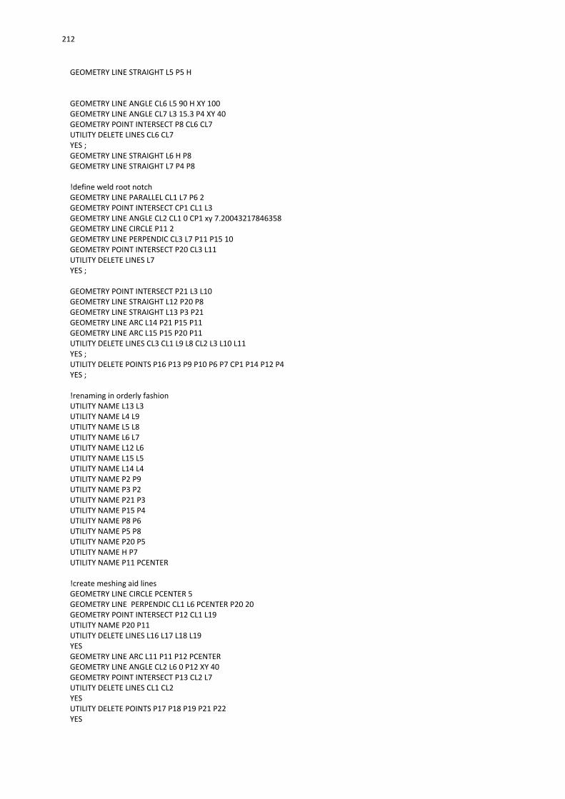
212
GEOMETRY LINE STRAIGHT L5 P5 H GEOMETRY LINE ANGLE CL6 L5 90 H XY 100 GEOMETRY LINE ANGLE CL7 L3 15.3 P4 XY 40 GEOMETRY POINT INTERSECT P8 CL6 CL7 UTILITY DELETE LINES CL6 CL7 YES ; GEOMETRY LINE STRAIGHT L6 H P8 GEOMETRY LINE STRAIGHT L7 P4 P8 !define weld root notch GEOMETRY LINE PARALLEL CL1 L7 P6 2 GEOMETRY POINT INTERSECT CP1 CL1 L3 GEOMETRY LINE ANGLE CL2 CL1 0 CP1 xy 7.20043217846358 GEOMETRY LINE CIRCLE P11 2 GEOMETRY LINE PERPENDIC CL3 L7 P11 P15 10 GEOMETRY POINT INTERSECT P20 CL3 L11 UTILITY DELETE LINES L7 YES ; GEOMETRY POINT INTERSECT P21 L3 L10 GEOMETRY LINE STRAIGHT L12 P20 P8 GEOMETRY LINE STRAIGHT L13 P3 P21 GEOMETRY LINE ARC L14 P21 P15 P11 GEOMETRY LINE ARC L15 P15 P20 P11 UTILITY DELETE LINES CL3 CL1 L9 L8 CL2 L3 L10 L11 YES ; UTILITY DELETE POINTS P16 P13 P9 P10 P6 P7 CP1 P14 P12 P4 YES ; !renaming in orderly fashion UTILITY NAME L13 L3 UTILITY NAME L4 L9 UTILITY NAME L5 L8 UTILITY NAME L6 L7 UTILITY NAME L12 L6 UTILITY NAME L15 L5 UTILITY NAME L14 L4 UTILITY NAME P2 P9 UTILITY NAME P3 P2 UTILITY NAME P21 P3 UTILITY NAME P15 P4 UTILITY NAME P8 P6 UTILITY NAME P5 P8 UTILITY NAME P20 P5 UTILITY NAME H P7 UTILITY NAME P11 PCENTER !create meshing aid lines GEOMETRY LINE CIRCLE PCENTER 5 GEOMETRY LINE PERPENDIC CL1 L6 PCENTER P20 20 GEOMETRY POINT INTERSECT P12 CL1 L19 UTILITY NAME P20 P11 UTILITY DELETE LINES L16 L17 L18 L19 YES GEOMETRY LINE ARC L11 P11 P12 PCENTER GEOMETRY LINE ANGLE CL2 L6 0 P12 XY 40 GEOMETRY POINT INTERSECT P13 CL2 L7 UTILITY DELETE LINES CL1 CL2 YES UTILITY DELETE POINTS P17 P18 P19 P21 P22 YES

213
GEOMETRY LINE STRAIGHT L12 P12 P13 GEOMETRY LINE ANGLE L10 L1 180 P11 XY 10 GEOMETRY LINE PERPENDIC CL1 L10 P23 PCENTER 10 GEOMETRY POINT INTERSECT P10 L3 CL1 UTILITY DELETE LINES CL1 YES GEOMETRY LINE STRAIGHT L13 P23 P10 UTILITY DELETE POINTS P24 YES GEOMETRY LINE STRAIGHT L14 P4 P11 GEOMETRY LINE STRAIGHT l15 P5 P12 UTILITY DELETE LINES L3 L7 YES GEOMETRY LINE STRAIGHT L3 P2 P10 GEOMETRY LINE STRAIGHT L7 P13 P7 GEOMETRY LINE STRAIGHT L16 P10 P3 GEOMETRY LINE STRAIGHT L17 P6 P13 UTILITY DELETE LINES L3 YES GEOMETRY POINT P16 10 25 0 GEOMETRY LINE STRAIGHT L20 P2 P16 GEOMETRY LINE STRAIGHT L3 P16 P10 GEOMETRY POINT P17 10 0 0 UTILITY DELETE LINES L1 YES GEOMETRY LINE STRAIGHT L1 P17 P9 GEOMETRY LINE STRAIGHT L18 P1 P17 GEOMETRY LINE STRAIGHT L19 P17 P16 !create surface GEOMETRY SURFACE 4SIDES SURF1 L1 +L9 L8 +L7 +L12 +L11 +L10 +L13
L3 L19 GEOMETRY SURFACE 4SIDES SURF2 L10 L14 +L4 L16 L13 GEOMETRY SURFACE 4SIDES SURF3 L11 L15 L5 L14 GEOMETRY SURFACE 4SIDES SURF4 L12 L17 L6 L15 GEOMETRY SURFACE 4SIDES SURF5 L18 L19 L20 L2 !boundary conditions PROPERTY BOUNDARY CONSTRAINT L8 1456 PROPERTY BOUNDARY CONSTRAINT L9 1456 !loading PROPERTY LOADS PRESSURE LO1 1 L2 ‐100 X !materials PROPERTY MATERIAL S1100 ELASTIC ISOTROP 210000 0.3 PROPERTY MATERIAL S890 ELASTIC ISOTROP 210000 0.3 PROPERTY MATERIAL S690 ELASTIC ISOTROP 210000 0.3 PROPERTY MATERIAL S460 ELASTIC ISOTROP 210000 0.3 PROPERTY ATTACH ALL MATERIAL S1100 !properties PROPERTY PHYSICAL TH1 GEOMETRY THINFSHL 1 PROPERTY ATTACH ALL TH1 !meshing CONSTRUCT SET SURFS APPEND SURFACES ALL MESHING TYPES SURF1 CQ16E MESHING TYPES SURF2 CQ16E MESHING TYPES SURF3 CQ16E MESHING TYPES SURF4 CQ16E MESHING TYPES SURF5 CQ16E

214
MESHING DIVISION LINE L1 90 MESHING DIVISION LINE L2 40 MESHING DIVISION LINE L3 ‐998 MESHING DIVISION LINE L4 10 MESHING DIVISION LINE L5 8 MESHING DIVISION LINE L6 660 MESHING DIVISION LINE L7 660 MESHING DIVISION LINE L8 10 MESHING DIVISION LINE L9 40 MESHING DIVISION LINE L10 248 MESHING DIVISION LINE L11 8 MESHING DIVISION LINE L12 660 MESHING DIVISION LINE L13 30 MESHING DIVISION LINE L14 530 MESHING DIVISION LINE L15 530 MESHING DIVISION LINE L16 ‐538 MESHING DIVISION LINE L17 30 MESHING DIVISION LINE L18 10 MESHING DIVISION LINE L19 40 MESHING DIVISION LINE L20 10 MESHING OPTIONS ALGORITHM PAVING SURF1 MESHING OPTIONS ALGORITHM MAPPED SURF2 MESHING OPTIONS ALGORITHM MAPPED SURF3 MESHING OPTIONS ALGORITHM MAPPED SURF4 MESHING OPTIONS ALGORITHM MAPPED SURF5 MESHING GENERATE ALL EYE FRAME