arX

iv:c

ond-

mat

/981

1110

v2

21

Jun

2000

HIGH TEMPERATURE RELAXATIONAL DYNAMICSIN

LOW-DIMENSIONAL QUANTUM FIELD THEORIES

Subir Sachdev

Department of Physics, Yale UniversityP.O. Box 208120, New Haven, CT 06520-8120, USA

Email: subir.sachdev@yale.edu

This paper presents a unified perspective on the results of two recent works(C. Buragohain and S. Sachdev cond-mat/9811083 and S. Sachdev cond-mat/9810399) along with additional background. We describe the low frequency,non-zero temperature, order parameter relaxational dynamics of a number of sys-tems in the vicinity of a quantum critical point. The dynamical correlations areproperties of the high temperature limit of renormalizable quantum field theoriesin spatial dimensions d = 1,2. We study, as a function of d and the numberof order parameter components, n, the crossover from the finite frequency, “am-plitude fluctuation”, gapped quasiparticle mode in the quantum paramagnet (orMott insulator), to the zero frequency “phase” (n ≥ 2) or “domain wall” (n = 1)relaxation mode near the ordered phase. Implications for dynamic measurementson the high temperature superconductors and antiferromagnetic spin chains arenoted.

Published inHighlights in Condensed Matter Physics,

APCTP/ICTP Joint International Conference,Seoul, Korea, June 12-16, 1998,

edited by B. K. Chung and M. VirasoroWorld Scientific, Singapore (2000).

Report No. cond-mat/9811110.

1 Introduction

Recent neutron scattering experiments by Aeppli et al.1 have studied the two-dimensional incommensurate spin correlations in the normal state of the hightemperature superconductor LaxSr1−xCuO4 at x ≈ 0.15 in some detail. Inparticular, they have determined the scattering cross section over a signifi-cant portion of the wavevector, frequency and temperature space. One oftheir striking observations has been that, while the dynamic structure factorof the electronic spins has quite an intricate functional form over this three-dimensional parameter space, the results become quite simple and explicablewhen interpreted in terms of the non-zero temperature dynamical properties

1

of a system in the vicinity of a quantum critical point 2,3. The data are consis-tent with such an interpretation over a decade in temperature and in over twodecades of the peak scattering amplitude, and indicate that there is a nearbyquantum critical point with dynamic critical exponent z ≈ 1. The nature of themeasured spin correlations indicates that this quantum critical point is the po-sition of a quantum phase transition to an insulating, charge- and spin-orderedground state. Varying the doping concentration, x, alone is not expected tobe sufficient to access this ordered state, and authors 1 asserted that a secondtuning parameter (‘y’) is necessary; e.g. it is known that replacing some of theSr by Nd allows one to move along the y axis 4.

In this paper, we will review recent theoretical work studying non-zerotemperature (T ) dynamical response functions closely related to those mea-sured in the neutron scattering experiment of Aeppli et al. 1 We will examinea simple class of models in spatial dimension d = 1, 2, which exhibit quantumordering transitions with z = 1. All of the models we shall study are closelyrelated to the following quantum field theory of a real, n-component, scalarfield φα (α = 1 . . .n):

ZQ =∫Dφα(x, τ) exp

(−∫ddx

∫ 1/T

0

dτ LQ

)

LQ =12

[1c2

(∂τφα)2 + (∇xφα)2 + (rc + r)φ2α

]+u

4!(φ2α

)2. (1)

Here we are using units with h̄ = kB = 1, x is the d-dimensional spatial co-ordinate, τ is imaginary time, c is a velocity, and rc, r and u are couplingconstants. The co-efficient of the φ2

α term (the ‘mass’ term) has been writtenas r+rc for convenience. The quartic non-linearity u makes ZQ as interactingquantum field theory, and it ultimately responsible for the dynamic relaxationphenomena we shall describe. For appropriate values of d and n, the model ZQexhibits a T = 0 quantum transition between an ordered phase with 〈φα〉 6= 0,and a quantum paramagnet with complete O(n) symmetry; the value of rcis chosen so that this transition occurs at r = 0. In physical applicationsof ZQ, the case n = 1 describes the Ising model in a transverse field, thecase n = 2 case describes a superfluid-insulator transition (with φ1 + iφ2, thecomplex superfluid order parameter), and n = 3 describes spin fluctuationsin a collinear quantum antiferromagnet (with φα the antiferromagnetic orderparameter).

We will be interested in the real-time dynamic properties of ZQ in thehigh T limit of the continuum quantum field theory (in some cases, this is alsothe ‘quantum critical’ region5). More specifically, in the vicinity of a quantum

2

critical point, the theory ZQ can be characterized by two distinct energy scales.The first, is a low energy scale, characterizing the deviation from the systemfrom the quantum critical point at r = 0: this varies as b|r|zν, where ν isthe correlation length exponent, and b is a non-universal, cutoff-dependentconstant needed to make the expression have physical units of energy; this lowenergy scale is the central quantity characterizing the continuum quantum fieldtheory. The second, is a high energy scale, and is of order cΛ, where Λ is ahigh-momentum cutoff needed at intermediate stages to define the continuumlimit of ZQ; this energy scale plays no role in the continuum quantum fieldtheory. We will be assuming here that the temperature is in between these twoenergy scales i.e.

b|r|zν � T � cΛ. (2)

We will characterize the response of the system by the dynamic suscepti-bility, χ(k, ωn), defined by

χ(k, ωn) ≡ 1n

∫ 1/T

0

dτ

∫ddx

n∑α=1

〈φα(x, τ)φα(0, 0)〉e−i(kx−ωnτ), (3)

where k is the wavevector, ωn the imaginary frequency; throughout we will usethe symbol ωn to refer to imaginary frequencies, while the use of ω will implythe expression has been analytically continued to real frequencies. Further,the static susceptibility, χ(k), is defined by

χ(k) ≡ χ(k, ωn = 0). (4)

We shall be especially interested here in a relaxation function R(k, ω), whichwe define as

R(k, ω) =1

χ(k)2ω

Imχ(k, ω). (5)

This is an even function of ω with the dimensions of time, and the Kramers-Kronig relation implies that ∫ ∞

−∞

dω

2πR(k, ω) = 1. (6)

After a Fourier transform to real time, R(k, t) (with R(k, t = 0) = 1) de-scribes the time-dependent relaxation of spin correlations at wavevector k dueto quantum and thermal fluctuations.

(In a regime where the predominant fluctuations have an energy muchsmaller than T , the low frequency dynamics becomes effectively classical, and

3

then the fluctuation-dissipation theorem implies that

R(k, ω) ≈ S(k, ω)S(k)

, (7)

where S(k, ω) is the dynamic structure factor, and S(k) is the equal-timestructure factor. However, this relationship is not generally true for a quantumsystem, and for clarity, we will always use (5) as our defining relation.)

The following sections will describe the behavior of R(k, ω) in the high Tlimit of the continuum quantum theory ZQ for various physically interestingcases in low dimensions: we will consider the case n = 1, d = 1 in Section 2,the case n = 3, d = 1 in Section 3, and all values of n in d = 2 in Section 4.

2 Ising chain in a transverse field

The Ising chain in a transverse field has the Hamiltonian

HI = −J∑i

(gσ̂xi + σ̂zi σ̂

zi+1

), (8)

where σ̂x,zi are Pauli matrices on the sites, i, of a d = 1 chain with latticespacing a. This model has a quantum critical point at g = 1, whose vicinityis believed to be described by the d = 1, n = 1 case of ZQ. Under thismapping, the field-theoretic correlators of φα under ZQ are equivalent to thelong-distance, long-time correlators of the order parameter σ̂z under the latticemodel HI .

The continuum high T dynamical response of (8) can be computed exactlyby a special trick relying on the conformal invariance of the critical theory atg = 1 6. The result for χ(k, ω) is

χ(k, ω) =Zc

T 7/4

GI(0)4π

Γ(7/8)Γ(1/8)

Γ(

116− iω + ck

4πT

)Γ(

116− iω − ck

4πT

)Γ(

1516− iω + ck

4πT

)Γ(

1516− iω − ck

4πT

) . (9)

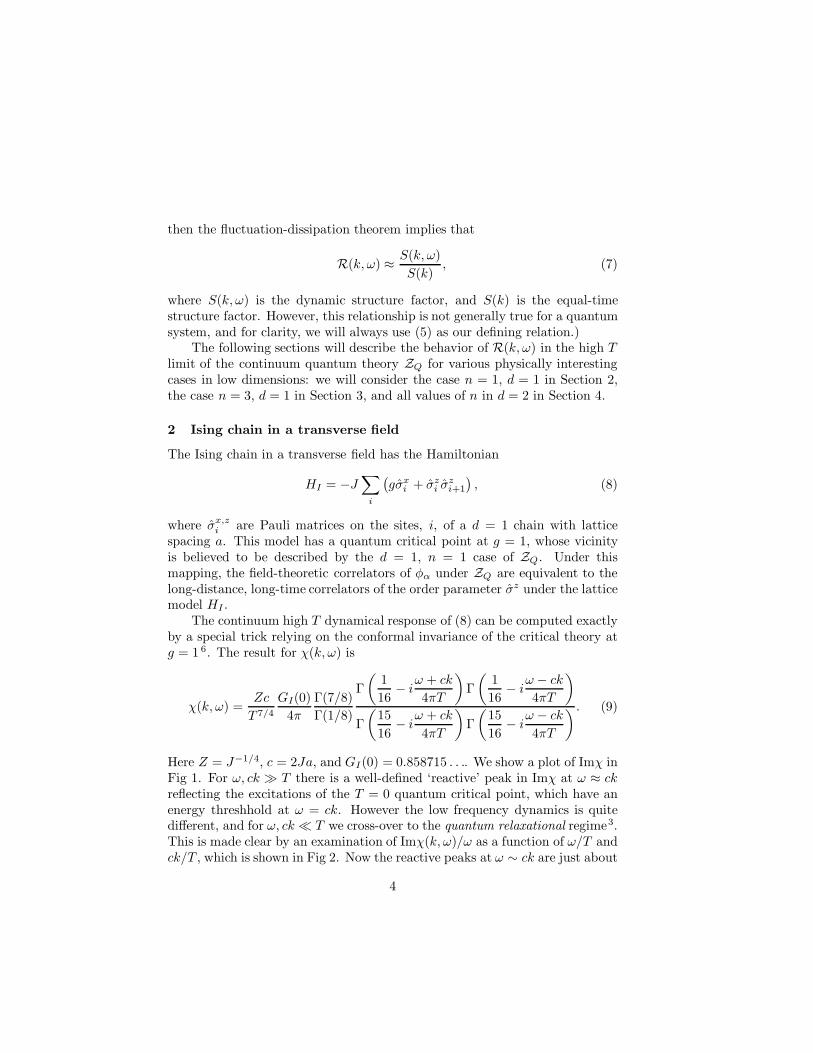
Here Z = J−1/4, c = 2Ja, and GI(0) = 0.858715 . . .. We show a plot of Imχ inFig 1. For ω, ck � T there is a well-defined ‘reactive’ peak in Imχ at ω ≈ ckreflecting the excitations of the T = 0 quantum critical point, which have anenergy threshhold at ω = ck. However the low frequency dynamics is quitedifferent, and for ω, ck� T we cross-over to the quantum relaxational regime3.This is made clear by an examination of Imχ(k, ω)/ω as a function of ω/T andck/T , which is shown in Fig 2. Now the reactive peaks at ω ∼ ck are just about

4

4

3

2

1

0

0

1

2

3

1.5

1

0.5

0

ω / T

ck / T

χImT7/4

Z

Figure 1: High temperature dynamic susceptibility, T 7/4Imχ(k, ω)/Z in (9) of the quantumIsing chain (d = 1, n = 1) as a function of ω/T and ck/T .

invisible, and the spectral density is dominated by a large relaxational peakat zero frequency. We can understand the structure of Fig 2 by expanding theinverse of (9) in powers of k and ω; this expansion has the form

χ(k, ω) =χ(0)

1− i(ω/ω1) + k2ξ̃2 − (ω/ω2)2, (10)

where χ(0) ∼ T−7/4, and ω1,2 and ξ̃ are parameters characterizing the expan-sion. For k not too large, the ω dependence in (10) is simply the response ofa strongly damped harmonic oscillator: this is the reason we have identifiedthe low frequency dynamics as “relaxational”. The function in (10) providesan excellent description of the spectral response in Fig 2. We determined thebest fit values of the parameters ω1,2 and ξ̃ by minimizing the mean squaredifference between the values of Imχ(k, ω)/ω given by (10) and (9) over therange 0 < ω < 2T and 0 < ck < 2T and obtained

ω1 = 0.396 Tω2 = 0.795 Tξ̃ = 1.280 c/T. (11)

5

2

1.5

1

0.5

0

0

0.5

1

1.5

2

6

4

2

0

ck / T

χω

ω / T

ImT11/4

Z

Figure 2: Plot of the spectral density of the quantum Ising chain (d = 1, n = 1)T 11/4Imχ(k, ω)/ωZ as a function of ω/T and ck/T . Note that this is simply the quan-tity in Fig 1 divided by ω. The reactive peaks at ω ≈ ck in Fig 1 are essentially invisible,and the plot is dominated by a large relaxational peak at zero wavevector and frequency.

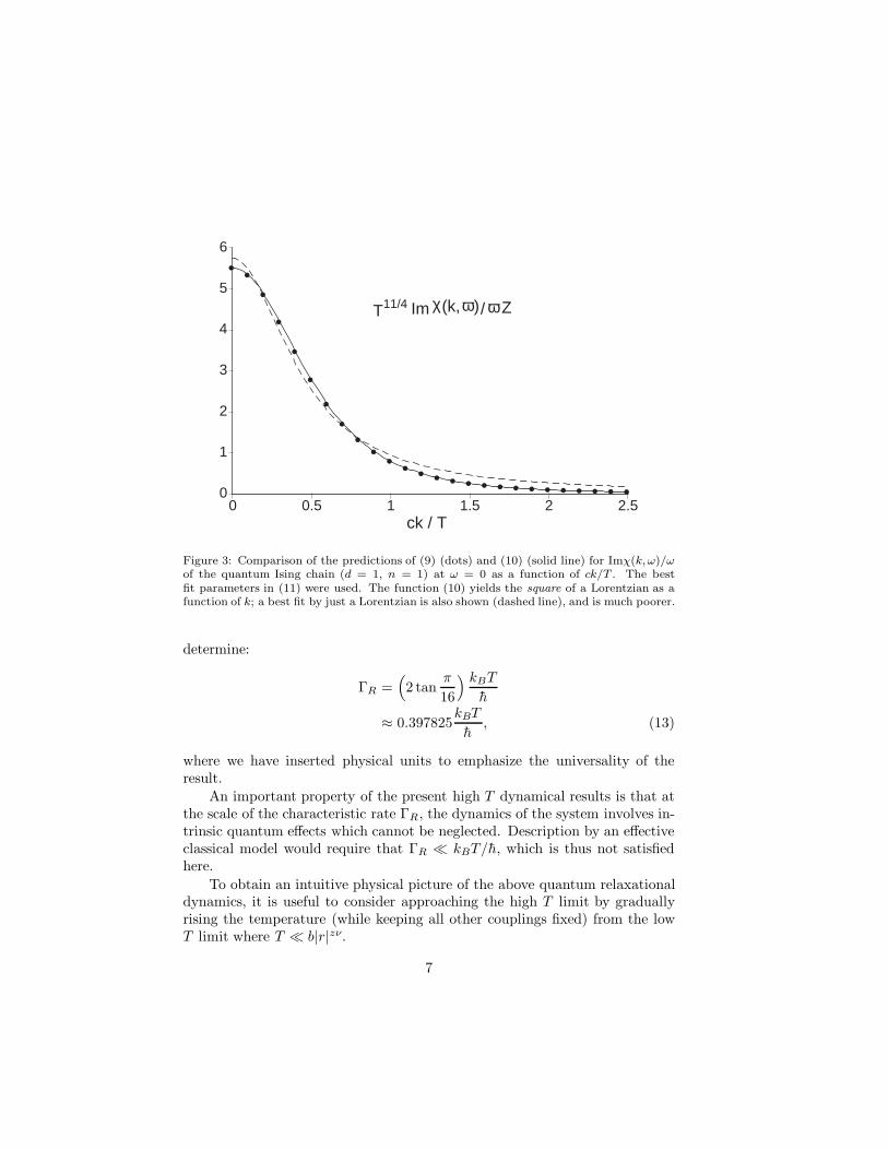
The quality of the fit is shown in Figs 3 and 4. In Fig 3 we compare thepredictions of (9) and (10) for Imχ(k, ω)/ω at ω = 0 as a function of ck/T . Theform (10) predicts a Lorentzian-squared response function and this is seen toprovide a better fit than a Lorentzian—a similar Lorentzian-squared responsewas used in analyzing the data in Ref. 1. In Fig 4 we plot the predictions of (9)and (10) for R(k, ω) at ck/T = 0, 1.5 as a function of ω/T . For k = 0 (ω = 0)there is a large overdamped peak at ω = 0 (k = 0), but a weak reactive peakat ω ∼ ck does make an appearance at larger wavevectors or frequencies.

For an alternative, and more precise, characterization of the relaxationaldynamics we can introduce the relaxation rate ΓR defined by

Γ−1R ≡

R(0, 0)2

; (12)

we have chosen this definition because for the suggestive functional form (10),ΓR = ω1, the frequency characterizing the damping. However, using (9) we

6

• ••

•

•

•

••••• • • • • • • • • • • • • • • •0

1

2

3

4

5

6

0 0.5 1 1.5 2 2.5

Im / ωT11/4 Zχ(k, )ω

ck / T

Figure 3: Comparison of the predictions of (9) (dots) and (10) (solid line) for Imχ(k,ω)/ωof the quantum Ising chain (d = 1, n = 1) at ω = 0 as a function of ck/T . The bestfit parameters in (11) were used. The function (10) yields the square of a Lorentzian as afunction of k; a best fit by just a Lorentzian is also shown (dashed line), and is much poorer.

determine:

ΓR =(

2 tanπ

16

) kBTh̄

≈ 0.397825kBT

h̄, (13)

where we have inserted physical units to emphasize the universality of theresult.

An important property of the present high T dynamical results is that atthe scale of the characteristic rate ΓR, the dynamics of the system involves in-trinsic quantum effects which cannot be neglected. Description by an effectiveclassical model would require that ΓR � kBT/h̄, which is thus not satisfiedhere.

To obtain an intuitive physical picture of the above quantum relaxationaldynamics, it is useful to consider approaching the high T limit by graduallyrising the temperature (while keeping all other couplings fixed) from the lowT limit where T � b|r|zν.

7

• ••

•

•

•

•••• • • • • • • • • • • • • • • •

• • • • • • • • • • • • • • • • • • • • • • • • •0

1

2

3

0 0.5 1 1.5 2 2.5 / Tω

ck/T = 0

ck/T = 1.5

R (k, )ω(T/ 2)

Figure 4: Comparison of the predictions of (9) (dots) and (10) (solid line) for the relaxationfunction (T/2)R(k,ω) of the quantum Ising chain (d = 1, n = 1) as a function of ω/T atck/T = 0,1.5.

First, consider the low T limit on the magnetically ordered side. Here theexcitations above the ground state are ‘domain walls’ which separate regionsin which the Ising order parameter has opposite signs. These domain walls canmove easily without significant change of energy, and their low energy motionleads to a large relaxational peak in R(k, ω) at ω = 0, k = 0 7. At very low T ,the domain walls are very dilute, and their spacing is much larger than theirthermal de Broglie wavelengths—consequently their motion can be described ina classical model. However, as T is raised into the high T regime, their spacingbecomes of order their de Broglie wavelength, and the relaxation rate of theircollisional dynamics becomes of order T : this is leads to the relaxational peakin Fig 4.

Second, we can begin by considering the low T limit on the quantumparamagnetic side. Now the excitations are local ‘flipped spins’ which requirea finite energy, ∆, to create them. So there is a sharp peak in R(k, ω) atω = ∆, which is broadened by collisions with the dilute, classical gas of pre-existing quasiparticles. In the language of the field φα, this finite frequencypeak arises from amplitude fluctuations in φ about a local minimum in itseffective potential. As T is raised, the quasiparticle gas becomes dense with

8

the mean-particle spacing becoming of order their de Broglie wavelength, thequasiparticle line-width becomes of order T , and the peak inR(k, ω) eventuallymoves to ω = 0.

3 Gapped, Heisenberg antiferromagnetic chains

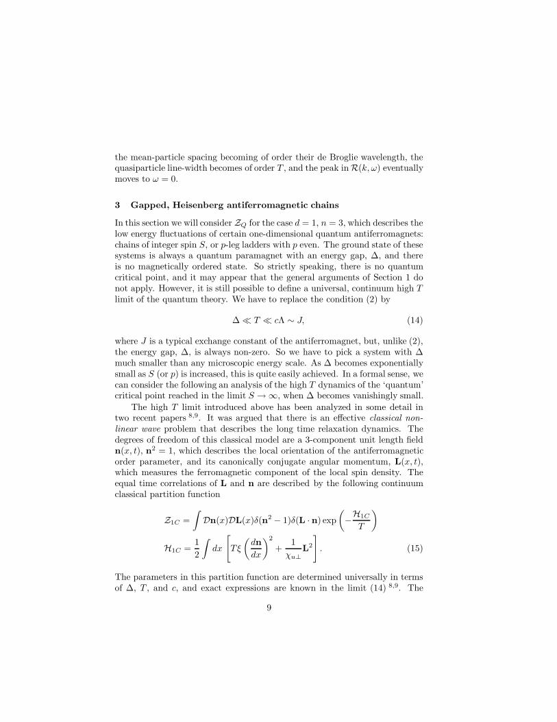
In this section we will consider ZQ for the case d = 1, n = 3, which describes thelow energy fluctuations of certain one-dimensional quantum antiferromagnets:chains of integer spin S, or p-leg ladders with p even. The ground state of thesesystems is always a quantum paramagnet with an energy gap, ∆, and thereis no magnetically ordered state. So strictly speaking, there is no quantumcritical point, and it may appear that the general arguments of Section 1 donot apply. However, it is still possible to define a universal, continuum high Tlimit of the quantum theory. We have to replace the condition (2) by

∆� T � cΛ ∼ J, (14)

where J is a typical exchange constant of the antiferromagnet, but, unlike (2),the energy gap, ∆, is always non-zero. So we have to pick a system with ∆much smaller than any microscopic energy scale. As ∆ becomes exponentiallysmall as S (or p) is increased, this is quite easily achieved. In a formal sense, wecan consider the following an analysis of the high T dynamics of the ‘quantum’critical point reached in the limit S →∞, when ∆ becomes vanishingly small.

The high T limit introduced above has been analyzed in some detail intwo recent papers 8,9. It was argued that there is an effective classical non-linear wave problem that describes the long time relaxation dynamics. Thedegrees of freedom of this classical model are a 3-component unit length fieldn(x, t), n2 = 1, which describes the local orientation of the antiferromagneticorder parameter, and its canonically conjugate angular momentum, L(x, t),which measures the ferromagnetic component of the local spin density. Theequal time correlations of L and n are described by the following continuumclassical partition function

Z1C =∫Dn(x)DL(x)δ(n2 − 1)δ(L · n) exp

(−H1C

T

)H1C =

12

∫dx

[Tξ

(dndx

)2

+1χu⊥

L2

]. (15)

The parameters in this partition function are determined universally in termsof ∆, T , and c, and exact expressions are known in the limit (14) 8,9. The

9

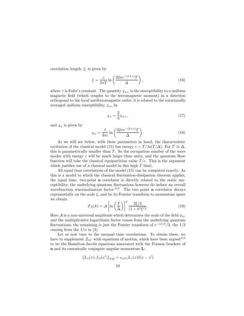
correlation length, ξ, is given by

ξ =c

2πTln(

32πe−(1+γ)T

∆

), (16)

where γ is Euler’s constant. The quantity χu⊥ is the susceptibility to a uniformmagnetic field (which couples to the ferromagnetic moment) in a directionorthogonal to the local antiferromagnetic order; it is related to the rotationallyaveraged uniform susceptibility, χu, by

χu =23χu⊥, (17)

and χu is given by

χu =1

3πcln(

32πe−(2+γ)T

∆

). (18)

As we will see below, with these parameters in hand, the characteristicexcitation of the classical model (15) has energy ε ∼ T/ ln(T/∆). For T � ∆,this is parametrically smaller than T . So the occupation number of the wavemodes with energy ε will be much larger than unity, and the quantum Bosefunction will take the classical equipartition value T/ε. This is the argumentwhich justifies use of a classical model in this high T limit.

All equal time correlations of the model (15) can be computed exactly. Asthis is a model to which the classical fluctuation-dissipation theorem applies,the equal time, two-point n correlator is directly related to the static sus-ceptibility; the underlying quantum fluctuations however do induce an overallwavefunction renormalization factor 8,9. The two point n correlator decaysexponentially on the scale ξ, and by its Fourier transform to momentum spacewe obtain

Tχ(k) = A[ln(T

∆

)]2 2ξ/3(1 + k2ξ2)

. (19)

Here A is a non-universal amplitude which determines the scale of the field φα,and the multiplicative logarithmic factor comes from the underlying quantumfluctuations; the remaining is just the Fourier transform of e−|x|/ξ/3, the 1/3coming from the 1/n in (3).

Let us now turn to the unequal time correlations. To obtain these, wehave to supplement Z1C with equations of motion, which have been argued 8,9

to be the Hamilton-Jacobi equations associated with the Poisson brackets ofn and its canonically conjugate angular momentum L:

{Lα(x), Lβ(x′)}PB = εαβγLγ(x)δ(x − x′)

10

{Lα(x), nβ(x′)}PB = εαβγnγ(x)δ(x− x′){nα(x), nβ(x′)}PB = 0. (20)

From this, and (15), we obtain directly the equations of motion for the quasi-classical waves

∂n∂t

= {n,H1C}PB

=1χu⊥

L× n

∂L∂t

= {L,H1C}PB

= (Tξ)n× ∂2n∂x2

. (21)

To compute the needed unequal time correlation functions, pick a set of initialconditions for n(x), L(x) from the ensemble (15). Evolve these deterministi-cally in time using the equations of motion (21). The value of the correlator isthen the product of the appropriate time-dependent fields, averaged over theset of all initial conditions. We also note here that simple analysis of the dif-ferential equations (21) shows that small disturbances about a nearly orderedn configuration travel with a characteristic velocity c(T ) given by

c(T ) = (Tξ(T )/χu⊥(T ))1/2, (22)

which is a basic relationship between thermodynamic quantities and the ve-locity c(T ). Notice from (16) and (18) that to leading logarithms c(T ) ≈ c,but this result is not satisfied by the subleading terms. The characteristic ex-citation will have energy ε ∼ c/ξ, and this leads to our estimate for ε madeearlier, when we justified the validity of a classical model.

The classical dynamics problem defined by (15) and (21) obeys that thecrucial property of being free of all ultraviolet divergences. Consequently, wemay determine its characteristic length and time scales by simple engineeringdimensional analysis, as no short distance cutoff scale is going to transforminto an anomalous dimension. Indeed, a straightforward analysis shows thatthis classical problem is free of dimensionless parameters, and is a unique,parameter-free theory. This is seen by defining

x =x

ξ

t =t

τϕ

11

L = L

√ξ

Tχu⊥, (23)

where the characteristic time, τϕ, is given by

τϕ =

√ξχu⊥T

; (24)

our notation suggests that τϕ (like Γ−1R earlier) is a phase coherence time be-

yond which relaxational dynamics of damped spin waves takes over. Inserting(23,24) into (15) and (21), we find that all parameters disappear and the par-tition function and equations of motion acquire a unique, dimensionless form,given by setting T = ξ = χu⊥ = 1 in them.

The above transformations allow us to easily obtain a scaling form for therelaxation function R:

R(k, ω) = τϕΨR(kξ, ωτϕ), (25)

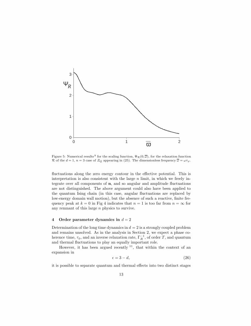
where ΨR is a universal scaling function, normalized as in (6). Further infor-mation on the structure of ΨR was obtained9 by a combination of analytic andnumerical methods. At sufficiently large kξ, we expect a pair of broadened,reactive, ‘spin-wave’ peaks at ω ≈ c(T )k (with c(T ) given in (22)), which aresimilar to those found in the high T limit of the quantum Ising chain in Fig 4.For the opposite limit of small kξ, we present numerical results for ΨR(0, ω)in Fig 5. There is a sharp relaxational peak at ω = 0, which is again similar tothat found in the high T limit of the quantum Ising chain in Fig 4. However,there is now a well-defined shoulder at ω ≈ 0.7 which was not found in theIsing case. This shoulder is a remnant of the large n result 3,10 which predictsa delta function at ω ∼ T/ ln(T/∆). So N = 3 is large enough for this finitefrequency oscillation to survive in the high T limit.

There is alternative, helpful way to view this oscillation frequency. Theunderlying degree of freedom in our dynamical field theory has a fixed ampli-tude, with |n| = 1. However, correlations of n decay exponentially on a lengthscale ξ—so if we imagine coarse-graining out to ξ, it is reasonable to expectsignificant amplitude fluctuations in the coarse-grained field. It is now usefulto visualize an effective field φα with no length constraint, which is just thefield we introduced in Section 1. On a length scale of order ξ, we expect theeffective potential controlling fluctuations of φα to have minimum at a non-zero value of |φα|, but to also allow fluctuations in |φα| about this minimum.The finite frequency in Fig 5 is due to the harmonic oscillations of φα aboutthis potential minimum, while the dominant peak at ω = 0 is due to angular

12

0

1

2

3

0 1 2ω

ΨR

Figure 5: Numerical results 9 for the scaling function, ΨR(0, ω), for the relaxation functionR of the d = 1, n = 3 case of ZQ appearing in (25). The dimensionless frequency ω = ωτϕ.

fluctuations along the zero energy contour in the effective potential. This isinterpretation is also consistent with the large n limit, in which we freely in-tegrate over all components of n, and so angular and amplitude fluctuationsare not distinguished. The above argument could also have been applied tothe quantum Ising chain (in this case, angular fluctuations are replaced bylow-energy domain wall motion), but the absence of such a reactive, finite fre-quency peak at k = 0 in Fig 4 indicates that n = 1 is too far from n = ∞ forany remnant of this large n physics to survive.

4 Order parameter dynamics in d = 2

Determination of the long time dynamics in d = 2 is a strongly coupled problemand remains unsolved. As in the analysis in Section 2, we expect a phase co-herence time, τφ, and an inverse relaxation rate, Γ−1

R , of order T , and quantumand thermal fluctuations to play an equally important role.

However, it has been argued recently 11, that within the context of anexpansion in

ε = 3− d, (26)

it is possible to separate quantum and thermal effects into two distinct stages

13

of the calculation, and to derive an effective classical wave model for the longtime dynamics. As in Section 3, we first derive an effective action for the staticsusceptibility, and then supplement it with equations of motion to obtain theunequal time correlations. We define the zero Matsubara frequency componentof φα by

Φα(x) = T

∫ 1/T

0

dτ φα(x, τ), (27)

and derive an effective action for Φα by integrating out the non-zero Matsubarafrequency components of φα. To leading non-trivial order in an expansion inε, this leads to the following effective action

Z2C =∫DΦα(x)DΠα(x) exp

(−H2C

T

)H2C =

∫ddx

{12

[c2Π2

α + (∇xΦα)2 + R̃Φ2α

]+U

4!(Φ2α

)2}. (28)

As in (15), along with the functional integral over Φα(x), we have includedan integral over a conjugate momentum field Πα(x) which will be importantfor our subsequent treatment of the dynamics; for now it easy to see thatthe Gaussian integral over Πα can be performed exactly, and it leaves thecorrelations of Φα under Z2C unchanged. The coupling constants in (28) areuniversally related to the underlying field theory ZQ controlling the quantumcritical point. Before specifying these, it is crucial to understand the nature ofthe ultraviolet divergences in Z2C considered as a classical field theory in itsown right. From standard field-theoretic analyses 12 it is known that Z2C hasonly one ultraviolet divergence, coming from a single one-loop tadpole graph inthe self energy: consequently, by trading the bare ‘mass’ R̃ for a renormalizedmass R defined by

R̃ = R− TU(n + 2

6

)∫ Λ ddk

(2π)d1

k2 +R, (29)

we can remove all cutoff dependencies in the correlators of Z2C (there aresome additional divergences, associated with composite operators, which ap-pear when two or more field operators approach each other in space: we willnot be concerned with these here). All observables of Z2C are then universalfunctions of the couplings R and U . Moreover, it is precisely these couplingsthat are universally computed from the underlying quantum field theory ZQ.Actually, instead to dealing with R and U as the two independent parameters

14

controlling correlators of Z2C , it is convenient to replace U by the dimension-less parameter G defined by

G ≡ TU

R(4−d)/2 , (30)

which is analogous to the Ginzburg parameter. In the high T limit (2), theseparameters were shown to have the following 13,11 universal values to leadingorder in ε

R = ε

(n+ 2n+ 8

)2π2(T/c)2

3

G =√ε

48π√

3√2(n+ 2)(n+ 8)

. (31)

As one lowers the temperature from the continuum high T limit, both R andG vary as universal functions of r/T 1/(zν): R decreases and G increases aswe lower the temperature into the magnetically ordered region (r < 0), whileR increases and G decreases as we lower the temperature into the quantumparamagnetic region (r > 0).

The values in (31) are the key to the argument justifying the use of aclassical dynamical model for small ε. From (28) it is clear that the charac-teristic Φα fluctuations have an energy of order c

√R ∼

√εT . As in Section 3,

this energy is parametrically smaller than T , and so the occupation numberof the relevant Φα will be given by their classical equipartition value. Thisalso means that the classical fluctuation dissipation theorem is obeyed, andthe static susceptibility, χ(k), computed from (28) by

Tχ(k) =1n

n∑α=1

〈|Φα(k)|2〉, (32)

is also the equal-time correlation of φα.We can now specify the recipe to compute the unequal time correlations

of φα, in manner which parallels Section 3. The fundamental Poisson bracketis

{Φα(x),Πβ(x′)}PB = δαβδ(x− x′), (33)

and the Hamiltonian H2C then leads to the Hamilton-Jacobi equations of mo-tion

∂Φα∂t

= {Φα(x),H2C}PB= c2Πα, (34)

15

and

∂Πα

∂t= {Πα(x),H2C}PB

= ∇2xΦα − R̃Φα −

U

6(Φ2

β)Φα, (35)

The equations (28), (34) and (35) define the central dynamical non-linear wavemodel of this section. We will compute correlations of the field Φα at unequaltimes, averaged over the set of initial conditions specified by (28). Notice allthe thermal ‘noise’ arises only in the random set of initial conditions. Thesubsequent time evolution is then completely deterministic, and precisely con-serves energy, momentum, and total O(n) charge. This should be contrastedwith the classical dynamical models studied in the theory of dynamic criti-cal phenomena 14,15, where there are explicit damping co-efficients, along withstatistical noise terms, in the equations of motion.

The dynamical model has been defined above in the continuum, and so weneed to consider the nature of its short distance singularities. As in Section 3,we assert11 that the only short distance singularities are those already presentin the equal time correlations analyzed earlier. These were removed by thesimple renormalization in (29), which is therefore adequate also for the unequaltime correlations. With this knowledge in hand, we can immediately writedown the universal scaling form obeyed by the relaxation function by simplearguments based upon analysis of engineering dimensions. The analog of (25)is now

R(k, ω) =1

c√R

ΨR

(k√R,ω

c√R,G), (36)

where ΨR is a universal function we wish to determine.It now remains to solve the dynamical problem specified by (28), (34) and

(35), and so determine ΨR. For small ε, the dimensionless strength of the non-linearity G in (31) is small; nevertheless we cannot use perturbation theory inG, because this fails in the low frequency limit. In other words, the dynamicalproblem remains strongly coupled even for small ε.

The only remaining possibility is to numerically solve the strong-couplingdynamical problem. Formally, we are carrying out an ε expansion, and sothe numerical solution should be obtained for d just below 3. However, itis naturally much simpler to simulate directly in d = 2, which is also thedimensionality of physical interest. Therefore, the approach to the solutionof the dynamic problem in the quantum critical region breaks down into twosystematic steps: (i) Use the ε = 3−d expansion to derive an effective classicalnon-linear wave problem13 characterized by the couplings R and G. (ii) Obtain

16

0

3

6

9

12

0 0.4 0.8 1.2 1.6ω

n=1

ΨR

Figure 6: Numerical results 11 for the zero momentum scaling function ΨR(0, ω,G) for therelaxation function,R, appearing in (36) for the d = 2, n = 1 model ZQ. The dimensionless

frequency ω = ω/c√R. Results are shown for G = 25 (dots), G = 30 (short dashes), G = 35

(long dashes) and G = 40 (full line). The high T limit value of G in (31) evaluates to G = 35.5at ε = 1 and n = 1.

the exact numerical solution11 of the classical non-linear wave problem at thesevalues ofR and G directly in d = 2. This division of the problem into two ratherdisjointed steps is also physically reasonable: it is primarily for the classicalthermal fluctuations that the dimensionality d = 2 plays a special role, andthe cases n = 1, 2 (which have non-zero temperature phase transitions abovethe magnetically ordered phase) and n ≥ 3 (which do not have a non-zerotemperature phase transition) are strongly distinguished—so it is importantto treat these exactly; on the other hand, the ε = 3− d expansion provides areasonable treatment of the quantum fluctuations down to d = 2 for all n.

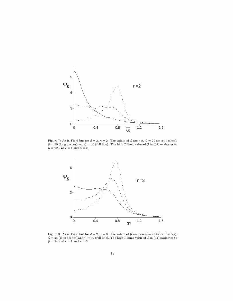
Figs 6–8 contain the results of a recent numerical computation of the scal-ing function in (36) at k = 0. These results are the analog of Fig 4 for theIsing chain and Fig 5 for the d = 1, n = 3 case. They show a consistent trendfrom small values of G and large values of n to large values of G and smallvalues of n, and we discuss the physical interpretation of the two limiting casesin turn.

For smaller G and larger n, we observe a peak in R(0, ω) at a non-zerofrequency. This peak is the remnant of a delta function obtained in the largen limit at a frequency ω ∼ T . In the present computation, it is clear thatthe peak is due to amplitude fluctuations as Φα oscillates about the mini-

17

0

3

6

9

0 0.4 0.8 1.2 1.6ω

n=2ΨR

Figure 7: As in Fig 6 but for d = 2, n = 2. The values of G are now G = 20 (short dashes),G = 30 (long dashes) and G = 40 (full line). The high T limit value of G in (31) evaluates toG = 29.2 at ε = 1 and n = 2.

0

3

6

0 0.4 0.8 1.2 1.6ω

n=3ΨR

Figure 8: As in Fig 6 but for d = 2, n = 3. The values of G are now G = 20 (short dashes),G = 25 (long dashes) and G = 30 (full line). The high T limit value of G in (31) evaluates toG = 24.9 at ε = 1 and n = 3.

18

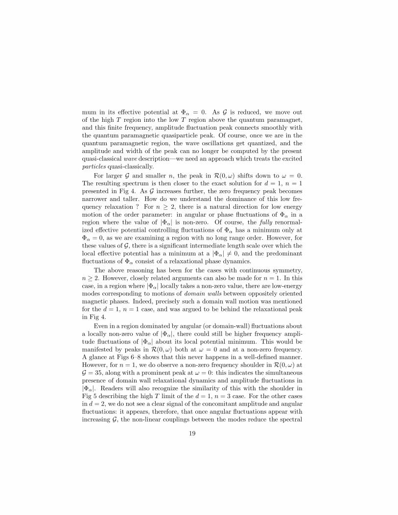
mum in its effective potential at Φα = 0. As G is reduced, we move outof the high T region into the low T region above the quantum paramagnet,and this finite frequency, amplitude fluctuation peak connects smoothly withthe quantum paramagnetic quasiparticle peak. Of course, once we are in thequantum paramagnetic region, the wave oscillations get quantized, and theamplitude and width of the peak can no longer be computed by the presentquasi-classical wave description—we need an approach which treats the excitedparticles quasi-classically.

For larger G and smaller n, the peak in R(0, ω) shifts down to ω = 0.The resulting spectrum is then closer to the exact solution for d = 1, n = 1presented in Fig 4. As G increases further, the zero frequency peak becomesnarrower and taller. How do we understand the dominance of this low fre-quency relaxation ? For n ≥ 2, there is a natural direction for low energymotion of the order parameter: in angular or phase fluctuations of Φα in aregion where the value of |Φα| is non-zero. Of course, the fully renormal-ized effective potential controlling fluctuations of Φα has a minimum only atΦα = 0, as we are examining a region with no long range order. However, forthese values of G, there is a significant intermediate length scale over which thelocal effective potential has a minimum at a |Φα| 6= 0, and the predominantfluctuations of Φα consist of a relaxational phase dynamics.

The above reasoning has been for the cases with continuous symmetry,n ≥ 2. However, closely related arguments can also be made for n = 1. In thiscase, in a region where |Φα| locally takes a non-zero value, there are low-energymodes corresponding to motions of domain walls between oppositely orientedmagnetic phases. Indeed, precisely such a domain wall motion was mentionedfor the d = 1, n = 1 case, and was argued to be behind the relaxational peakin Fig 4.

Even in a region dominated by angular (or domain-wall) fluctuations abouta locally non-zero value of |Φα|, there could still be higher frequency ampli-tude fluctuations of |Φα| about its local potential minimum. This would bemanifested by peaks in R(0, ω) both at ω = 0 and at a non-zero frequency.A glance at Figs 6–8 shows that this never happens in a well-defined manner.However, for n = 1, we do observe a non-zero frequency shoulder in R(0, ω) atG = 35, along with a prominent peak at ω = 0: this indicates the simultaneouspresence of domain wall relaxational dynamics and amplitude fluctuations in|Φα|. Readers will also recognize the similarity of this with the shoulder inFig 5 describing the high T limit of the d = 1, n = 3 case. For the other casesin d = 2, we do not see a clear signal of the concomitant amplitude and angularfluctuations: it appears, therefore, that once angular fluctuations appear withincreasing G, the non-linear couplings between the modes reduce the spectral

19

weight in the amplitude mode to a negligible amount.It is interesting to examine the above results at the value of high T limit

for G in (31) evaluated directly in ε = 1. We find G = 35.5, 29.2, 24.9 forn = 1, 2, 3, and these values are very close to the position where the crossoverbetween the above behaviors occurs. The n = 1 case has a clear maximumin R(0, ω) at ω = 0 (along with a finite frequency shoulder), while there is amore clearly defined finite frequency peak for n = 3.

In closing, we note that there is a passing resemblance between the abovecrossover in dynamical properties as a function of G, and a well-studied phe-nomenon in dissipative quantum mechanics 18,19,20: the crossover from ‘coher-ent oscillation’ to ‘incoherent relaxation’ in a two-level system coupled to aheat bath . However, here we do not rely on an arbitrary heat bath of lin-ear oscillators, and the relaxational dynamics emerges on its own from theunderlying Hamiltonian dynamics of an interacting many-body, quantum sys-tem. Our description of the crossover has been carried out in the context of aquasi-classical wave model here, but, as we noted earlier, the ‘coherent’ peakconnects smoothly to the quasiparticle peak in low T paramagnetic region—here the wave oscillations get quantized into discrete lumps which must thenbe described by a ‘dual’ quasi-classical particle picture.

5 Conclusions

We have described the high temperature relaxational dynamics for a numberof models in spatial dimensions d = 1, 2. This dynamics is a property of arenormalizable, interacting continuum quantum field theory. Two cases canbe further distinguished:(i) The excitations of the theory retain a non-zero scattering amplitude at highenergies and temperatures: the models of Section 2 and 4 are of this type. Forthese, the only characteristic energy scale controlling the density and interac-tion strength of the excitations becomes T itself, and so the phase coherencetime, and the inverse relaxation rate, are universal numbers times h̄/kBT . Asa result, quantum and thermal fluctuations contribute equally to the phaserelaxation. (However, in Section 4 we did develop an expansion in which theuniversal prefactors of h̄/kBT became numerically large and so the long timerelaxation was described by an effective classical model.)(ii) The theory becomes asymptotically free at high energies, and so the scat-tering amplitude of the excitations vanishes at large T . The model of Section 3is of this class, and has a phase coherence time and inverse relaxation rate oforder (h̄/kBT ) ln(kBT/∆), where ∆ is an energy scale characterizing the lowenergy theory. These times are parametrically larger than h̄/kBT and so the

20

relaxational dynamics is classical.We have developed a fairly complete description of the dynamical corre-

lations of these models, and our results should be testable in experiments oncompounds the cuprate superconductor family, Heisenberg spin chains, anddouble layer quantum Hall systems 16,17.

Acknowledgments

The results in Section 3 grew out of collaborations with Kedar Damle 8 andChiranjeeb Buragohain 9.

Portions of this review have been adapted from “Quantum Phase Transi-tions”, by S. Sachdev, Cambridge University Press, in press. I am grateful tothe Press for permission to use this material here.

I thank Professors Yunkyu Bang, Y. M. Cho, Jisoon Ihm, Jaejun Yu andLu Yu for the opportunity to attend this stimulating conference, and for theirhard work in making it a great success. This research was supported by NSFGrant No DMR 96–23181.

References

[1] G. Aeppli, T. E. Mason, S. M. Hayden, H. A. Mook, and J. Kulda,Science 278, 1432 (1998).

[2] S. Sachdev, and J. Ye, Phys. Rev. Lett. 69, 2411 (1992).[3] A. V. Chubukov, S. Sachdev, and J. Ye Phys. Rev. B 49, 11919 (1994).[4] J. M. Tranquada, J. D. Axe, N. Ichikawa, A. R. Moodenbaugh, Y. Naka-

mura and S. Uchida Phys. Rev. Lett. 78, 338 (1997).[5] S. Chakravarty, B. I. Halperin, and D. R. Nelson, Phys. Rev. B 39, 2344

(1989).[6] S. Sachdev in Proceedings of the 19th IUPAP International Conference

on Statistical Physics, Xiamen, China, ed. B.-L. Hao, (World Scientific,Singapore, 1996); cond-mat/9508080.

[7] S. Sachdev and A. P. Young, Phys. Rev. Lett. 78, 2220 (1997).[8] K. Damle and S. Sachdev, Phys. Rev. B 57, 8307 (1998).[9] C. Buragohain and S. Sachdev, cond-mat/9811083.[10] Th. Jolicoeur and O. Golinelli, Phys. Rev. B 50, 9265 (1994).[11] S. Sachdev, cond-mat/9810399.[12] P. Ramond, Field Theory, A Modern Primer (Benjamin-Cummings,

Reading, 1981).[13] S. Sachdev, Phys. Rev. B 55, 142 (1997).[14] B. I. Halperin, P. C. Hohenberg, and S. k. Ma, Phys. Rev. Lett. 29,

1548 (1972); Phys. Rev. B 10, 139 (1974).

21

[15] P. C. Hohenberg and B. I. Halperin, Rev. Mod. Phys. 49, 435 (1977).[16] V. Pellegrini, A. Pinczuk, B. S. Dennis, A. S. Plaut, L. N. Pfeiffer, and

K. W. West Science 281, 799 (1998).[17] S. Das Sarma, S. Sachdev, and L. Zheng, Phys. Rev. B 58, 4672 (1998).[18] A. J. Leggett, S. Chakravarty, A. T. Dorsey, M. P. A. Fisher, A. Garg,

and W. Zwerger, Rev. Mod. Phys. 59, 1 (1987).[19] U. Weiss, Quantum Dissipative Systems (World Scientific, Singapore,

1993).[20] F. Lesage and H. Saleur, Nucl. Phys. B 493, 613 (1997).

22