Journal of Real-Time Image Processing manuscript No.(will be inserted by the editor)

Ahmet Oguz Akyuz

High Dynamic Range Imaging Pipeline on the GPU

Received: date / Revised: date

Abstract Use of high dynamic range (HDR) images andvideo in image processing and computer graphics appli-cations is rapidly gaining popularity. However, creatingand displaying high resolution HDR content on CPUsis a time consuming task. Although some previous workfocused on real-time tone mapping, implementation ofa full HDR imaging (HDRI) pipeline on the GPU hasnot been detailed. In this article we aim to fill this gapby providing a detailed description of how the HDRIpipeline, from HDR image assembly to tone mapping,can be implemented exclusively on the GPU. We alsoexplain the trade-offs that need to be made for improv-ing efficiency and show timing comparisons for CPU vs.GPU implementations of the HDRI pipeline.

1 Introduction

The use of high dynamic range imagery in computergraphics and image processing has gained popularity inrecent years. This can be attributed to the increased re-alism and visual quality that is afforded by use of HDRdata. Techniques such as image-based lighting, environ-ment mapping, and special effects such as realistic mo-tion blur and the well known bloom effect all produceimproved results if they use HDR data instead of lowdynamic range (LDR) data (Reinhard et al 2010).

This increased demand for working with HDR con-tent is well matched with the capabilities of moderngraphics cards. Currently all modern graphics hardwaresupport floating point textures and renderbuffers. Thisallows programmers to directly feed in a floating pointHDR image and process it on the GPU.

It is, however, often the case that HDR images used ingraphics applications are created offline using the CPU,or they are obtained as pre-made from external imagedatabases (Debevec 1998). However, given the large num-ber of independent pixel operations required to create

A. O. AkyuzMiddle East Technical University, Turkey

an HDR image, the process of HDRI assembly is verysuitable to be implemented on the GPU. Thus, the firstgoal of this paper is to demonstrate how to create anHDR image from a set of bracketed low dynamic range(e.g. JPEG) images directly on the GPU by using theOpenGL API.

Due to the limitations of conventional display de-vices, it is not possible to display HDR imagery directly,although this may change in near future as HDR dis-plays enter the mainstream (Seetzen et al 2004; Akyuzet al 2007). Instead, their dynamic range needs to be re-duced followed by quantization into an integer 8-bit percolor channel data type before they can be shown on adisplay device. Algorithms that perform dynamic rangereduction are called tone mapping (or tone reproduction)operators (TMOs), and they range from simple linearscaling to sophisticated multi-scale approaches that at-tempt to simulate the human vision (see Devlin (2002);Reinhard et al (2010); Banterle et al (2011) for excellentreviews).

Similar to the HDR assembly process, most TMOsare comprised of a large number of independent pixeloperations which render them suitable for a GPU im-plementation as well. One of the most popular TMOsthat belongs to this category is the photographic tonereproduction operator (Reinhard et al 2002). Thus, thesecond goal of this paper is to demonstrate how boththe global and local versions of this operator can be effi-ciently implemented by using OpenGL fragment shaders.Different from previous work, we will show that the im-plementation of this operator neither requires expensiveconvolution nor Fourier transform operations to computelocal adaptation luminances.

2 Related Work

In this section, we review the previous work that dealswith optimizing the HDR imaging pipeline. Cohen et al(2001) introduced the idea of HDR texture mapping onthe GPU. As contemporary graphics cards at the time

2

Fig. 1: A bracketed sequence captured with a Canon EOS 550D/T2i digital camera. Each exposure is 1-fstop apart from thenext exposure in the series.

of the study did not support floating point textures, theauthors proposed a technique to simulate HDR texturesby using multiple 8-bit textures. Battiato et al (2003),on the other hand, provided a state-of-the-art report ofthe HDRI pipeline from HDR image creation to tonemapping. However, implementation of the pipeline onthe GPU was not discussed.

The idea of tone mapping on the GPU was intro-duced by several authors (Goodnight et al 2003; Artusiet al 2003; Goodnight et al 2005). In Goodnight et al(2003) and Goodnight et al (2005), the authors imple-mented Reinhard et al (2002)’s tone mapping operatorusing fragment shaders. To implement the local versionof this operator, they have devised an efficient GPUbased convolution operation. Furthermore, the authorshave shown how to apply the method to time-varyingsequences such as HDR videos. Artusi et al (2003), onthe other hand, proposed a general framework to speed-up global tone mapping operators by effectively dividingthe workload between the CPU and the GPU.

A real-time tone mapping operator that also mod-els the perception effects was developed by Krawczyket al (2005). In this work, the authors modeled severalimportant effects such as visual acuity, glare, and lumi-nance adaptation. Later work implemented a Reinhard-like operator on FPGA architectures (Hassan and Car-letta 2007b,a).

To summarize, previous studies made significant con-tributions to achieve real-time performance in tone map-ping. In this work, however, we explain how the full HDRimaging pipeline, from image creation to display, can beimplemented in real-time. Different from previous work,we also show how a local tone mapping operator thatutilizes local adaptation luminances can be implementedwithout having to implement neither convolution norFourier transform based approaches on the GPU.

3 Theory

In this section, we will briefly explain the theory be-hind the HDR image generation and tone mapping. Their

Fig. 2: The combined result of the sequence in Figure 1 into asingle HDR image which is tone mapped using the techniquedescribed in this paper.

GPU implementation will be discussed in the followingsection.

3.1 HDR Image Assembly

HDR images can be created in several ways: direct cap-ture, rendering, and multiple exposures technique areamong the most commonly used ones. Direct capturemay become the de facto way of creating HDR imagesin future, but currently it requires special hardware fur-nished with HDR sensors and therefore is not commonlyused by most photographers. Furthermore, most such de-vices impose other restrictions such as limited resolution,long capture times, and lack of color support (Reinhardet al 2010). Rendering, on the other hand, is only suitablefor computer generated HDR imagery.

The multiple exposures technique allows photogra-phers to take a bracketed sequence of LDR images usinga conventional digital camera, and then merge them intoa single HDR image. Figure 1 depicts such a sequence of9 exposures with each exposure 1-fstop apart from thenext one. In that each exposure is properly exposed for

3

a different region in the scene, the final HDR image con-tains details in both dark and light regions (Figure 2).Owing to the fact that this technique allows generationof HDR images using off-the-shelf cameras, it is a popu-lar choice among photographers.

A single pixel, Ij , of an HDR image can be computedby using the following formula in the multiple exposurestechnique:

Ij =

N∑

i=1

f−1(pij)w(pij)

ti

/

N∑

i=1

w(pij), (1)

where N is the number of LDR images, pij is the value ofpixel j in image i, f is the camera response function, w isa weighting function used to attenuate the contributionof poorly exposed pixels, and ti is the exposure time ofimage i. One can obtain an HDR image by computingthis equation for all pixels.

In this equation, the inverse of the camera responsefunction, f−1, is used to linearize (i.e. degamma) theLDR images as they are typically captured in the non-linear sRGB color space. f−1 can be recovered directlyfrom the bracketed sequence using response curve recov-ery algorithms (Debevec and Malik 1997; Mitsunaga andNayar 1999; Robertson et al 2003), or it can be assumedto match the sRGB standard. We adopt the latter ap-proach in this paper to benefit from OpenGL’s sRGBtexture support.

3.2 Dynamic Range Reduction

Standard display devices such as televisions and com-puter monitors are designed to display 8-bit per colorchannel integer input streams (although video cards thatcan output 10-bit and monitors that can display themhave been in use for some time (AMD 2008)). Due tothis limitation, HDR images and video cannot be di-rectly displayed on standard display devices. To displaythem, their dynamic range needs to be reduced followedby quantization into 8-bit integers. The algorithms thatperform this task are called tone mapping (or tone re-production) operators1.

To date, various tone mapping operators have beenproposed each with a different approach to dynamic rangereduction. TMOs are generally classified as global and lo-cal with global operators applying the same compressivefunction to each pixel while local operators changing theshape of this function (thus the degree of compression)based on the statistics of the local neighborhood aroundeach pixel.

One of the most popular TMOs that is commonlyused in practice, and that ranks high in user studies, isReinhard et al.’s photographic tone reproduction oper-ator (Reinhard et al 2002). This operator comes in twoflavors, namely the global and the local operator.

1 Quantization into 8-bits is not part of tone mapping, butit is a necessary step to create displayable images.

3.2.1 Global Operator

The global operator starts by computing the key of thescene which indicates its overall subjective brightness.The key is approximated by the log-average luminance(see Section 3.3 for color space conversions needed toobtain luminance from color and vice-versa), Lw:

Lw = exp( 1

N

∑

x,y

log(δ + Lw(x, y)))

. (2)

Here, Lw(x, y) indicates the world luminance2 of pixel(x, y) and δ is a small offset added to avoid singularitythat may occur at log(0) if black pixels are present inthe image. The summation is performed across the entireimage.

Once the log-average luminance is computed, it ismapped to a user defined value, a, based on the desiredsubjective brightness of the scene. This is accomplishedby:

L(x, y) =a

Lw

Lw(x, y). (3)

For most scenes illuminated by moderate lighting, a canbe set to 0.18. To render darker scenes, it may be reducedto 0.09 or 0.045 (or less), and for lighter scenes it maybe increased to 0.36 or 0.72 (or more).

Once the image is scaled in this manner, the actualdynamic range compression is performed using a sig-moidal compression function:

Ld(x, y) =L(x, y)

1 + L(x, y), (4)

where Ld(x, y) represents the display luminance. Whilethis equation is guaranteed to bring all pixels into a dis-playable range, some intentional burning in bright areasmay be desired to create a more natural photographiclook. The amount of burning can be controlled by a userdefined parameter, Lwhite:

Ld(x, y) =L(x, y)(1 + L(x,y)

L2

white

)

1 + L(x, y). (5)

In this final equation, all luminance values greater thanLwhite will be mapped to 1; that is they will burn out.If Lwhite is set to infinity, this equation will reduce toEquation 4.

2 The subscript w indicates world luminance which may bein absolute or relative units depending on the calibration ofthe image.

4

3.2.2 Local Operator

The local operator resembles the global operator in thattone mapping is performed via a similar formula:

Ld(x, y) =L(x, y)

1 + V1(x, y, s). (6)

The difference, however, is that V1 represents the localadaptation luminance in the neighborhood around thepixel (x, y). The size of this neighborhood is controlledby the scale parameter, s. Vi can be computed as

Vi(x, y, s) = L(x, y)⊗Ri(x, y, s), (7)

where Ri is a Gaussian profile of the form

Ri(x, y, s) =1

π(αis)2exp

(

−x2 + y2

(αis)2

)

. (8)

To determine the appropriate scale, Reinhard et al(2002) propose to compute the difference of Gaussianconvolutions at different scales, V1 and V2. When thedifference between the two convolution results is above athreshold, the appropriate scale is found. This, in effect,computes the largest uniform region around each pixel,which serves as an adaptation region for that pixel. Thiscan be formalized as:

V (x, y, s) =V1(x, y, s)− V2(x, y, s)

2φa/s2 + V1(x, y, s), (9)

where φ is a sharpening parameter. Here the goal is tofind the largest scale sm that satisfies:

|V (x, y, sm)| < ǫ, (10)

where ǫ is a user parameter. Larger values give rise tolarger adaptation neighborhoods. Reinhard et al (2002)suggests using φ = 8.0 and ǫ = 0.05 as default parame-ters.

The photographic tone mapping operator poses twochallenges for a GPU implementation. First, the log-average luminance of the whole image needs to be com-puted - an operation which is not GPU friendly. Sec-ond, local adaptation luminances need to be computedfor the local operator. This amounts to convolving theimage with filters of varying sizes, which is also not aGPU friendly operation. In this paper, we show that bothproblems can be solved by judicious use of mipmapping.

3.3 Dealing with Color

The dynamic range compression described in the previ-ous section expects luminance values as input. However,in practice, we typically deal with color images. To con-vert color values to luminance, we need to employ colorspace transformations. After tone mapping we can in-vert these transformations to retrieve the modified color

values. In this section, we briefly highlight the key fea-tures of these color space transformations. For a morecomplete treatment, we refer the reader to literature oncolor imaging (Wyszecki and Stiles 2000; Reinhard et al2008).

To compute the luminance value for a given colortriplet, we first need to know its color space. If this in-formation is not available, we can assume that the HDRimage is in the sRGB color space as this is the defaultoutput color space for most digital cameras. We also as-sume that the HDR image contains linear color values.This is also a reasonable assumption as the HDR gen-eration process typically linearizes the individual expo-sures before combining them into the HDR image. Wecan then convert an sRGB color value into its CIE XYZrepresentation with the following transformation (ITU2002):

Xw

Yw

Zw

=

0.4124 0.3576 0.18050.2126 0.7152 0.07220.0193 0.1192 0.9505

Rw

Gw

Bw

. (11)

In the CIE XYZ color space, the Y component encodesthe luminance. Thus, Yw is equal to the world luminanceLw that we used in the previous section. We can nowcompress Yw to obtain the display luminance Yd whichis equal to Ld in Equations 4 and 5.

The output RGB colors can be computed by:

Cd =

(

Cw

Yw

)c

Yd (12)

where C = R,G,B and c is used for optional satura-tion adjustment. Setting c > 1 increases saturation whilec < 1 decreases it. It is worth noting that all of thesetransformations described in this section are performedfor each pixel independently, and thus are very amenableto benefit from GPU implementation.

4 Mipmapping

As mipmapping constitutes a key part of our algorithmwhich we use to compute the global average, Lw, andlocal adaptation luminances, V1 and V2, a brief review ofthe concept can be useful. Mipmapping, first introducedby Williams (1983), is a commonly used technique tomap texture images onto polygonal surfaces. The ideaof mipmapping is to store a texture image as a pyra-mid of multiple levels, where each level contains a pro-gressively lower-resolution version of the original image.During texture mapping, the level which most closelymatches the screen size of the polygon that is being tex-tured is chosen as the source image.

In OpenGL, the mipmap levels for two dimensionaltextures can be explicitly provided by the programmerusing glTexImage2D or glTexSubImage2D calls. Alter-natively, the programmer can request automatic gener-ation of mipmaps from the OpenGL server by using the

5

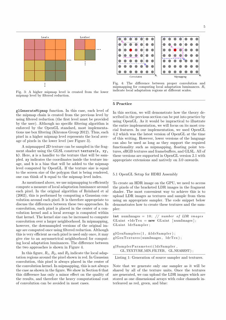
Fig. 3: A higher mipmap level is created from the lowermipmap level by filtered reduction.

glGenerateMipmap function. In this case, each level ofthe mipmap chain is created from the previous level byusing filtered reduction (the first level must be providedby the user). Although no specific filtering algorithm isenforced by the OpenGL standard, most implementa-tions use box filtering (Khronos Group 2012). Thus, eachpixel in a higher mipmap level represents the local aver-age of pixels in the lower level (see Figure 3).

A mipmapped 2D texture can be sampled in the frag-ment shader using the GLSL construct texture(s, xy,b). Here, s is a handler to the texture that will be sam-pled. xy indicates the coordinates inside the texture im-age, and b is a bias that will be added to the mipmaplevel computed by OpenGL. If the texture size is equalto the screen size of the polygon that is being rendered,one can think of b equal to the mipmap level index.

As mentioned above, we use mipmapping to efficientlycompute a measure of local adaptation luminance aroundeach pixel. In the original algorithm of Reinhard et al(2002), this is performed by computing a Gaussian con-volution around each pixel. It is therefore appropriate todiscuss the differences between these two approaches. Inconvolution, each pixel is placed in the center of a con-volution kernel and a local average is computed withinthat kernel. The kernel size can be increased to computeconvolution over a larger neighborhood. In mipmapping,however, the downsampled versions of the original im-age are computed once using filtered reduction. Althoughthis is very efficient as each pixel is used only once, it maygive rise to an asymmetrical neighborhood for comput-ing local adaptation luminances. The difference betweenthe two approaches is shown in Figure 4.

In this figure, R1, R2, and R3 indicate the local adap-tation regions around the pixel shown in red. In Gaussianconvolution, this pixel is always placed in the center ofthe convolution kernel. In mipmapping, this is not alwaysthe case as shown in the figure. We show in Section 6 thatthis difference has only a minor effect on the quality ofthe results, and therefore the heavy computational costof convolution can be avoided in most cases.

Fig. 4: The difference between proper convolution andmipmapping for computing local adaptation luminances. Ri

indicate local adaptation regions at different scales.

5 Practice

In this section, we will demonstrate how the theory de-scribed in the previous section can be put into practice byusing OpenGL. As it would be impractical to illustratethe entire implementation, we will focus on its most cru-cial features. In our implementation, we used OpenGL4.2 which was the latest version of OpenGL at the timeof this writing. However, lower versions of the languagecan also be used as long as they support the requiredfunctionality such as mipmapping, floating point tex-tures, sRGB textures and framebuffers, and GLSL. All ofthese versions are supported in OpenGL version 2.1 withappropriate extensions and natively on 3.0 onwards.

5.1 OpenGL Setup for HDRI Assembly

To create an HDR image on the GPU, we need to accessthe pixels of the bracketed LDR images in the fragmentshader. The most convenient way to achieve this is toupload LDR images as textures and sample from themusing an appropriate sampler. The code snippet belowdemonstrates how to create these textures and the sam-pler:

int numImages = 10 ; // number o f LDR images

GLuint ∗ ldrTex = new GLuint [ numImages ] ;

GLuint ldrSampler ;

glGenSamplers (1 , &ldrSampler ) ;

glGenTextures ( numImages , ldrTex ) ;

g lSamplerParameter i ( ldrSampler ,

GL TEXTURE MIN FILTER, GL NEAREST) ;

Listing 1: Generation of source sampler and textures.

Note that we generate only one sampler as it will beshared by all of the texture units. Once the texturesare generated, we can upload the LDR images which arestored as one dimensional arrays with color channels in-terleaved as red, green, and blue:

6

for ( int i = 0 ; i < numImages ; ++i ) {

glBindTexture (GL TEXTURE 2D, ldrTex [ i ] ) ;

glTexImage2D (GL TEXTURE 2D, 0 , GL SRGB8,

w, h , 0 , GL RGB, GL UNSIGNED BYTE,

ldrImg [ i ] ) ;

}

Listing 2: Uploading of LDR images into textures.

Here, w and h denote the dimensions of the LDR images.It is important to note that the internal format of thetextures is set to sRGB. This will allow us to retrievethe linearized color values when we sample from thesetextures in the fragment shader. In other words, sam-pling from an sRGB texture will approximate the resultof f−1(pij) in Equation 1.

We can now set up the source texture and samplerbindings. First, we need to bind the LDR sampler into allof the texture units as we want to use the same samplerfor all units. Second, we need to bind each LDR textureinto a different texture unit to be able to access themsimultaneously in the fragment shader. These settingscan be achieved by:

GLint ldrSamplerUnits [ 1 6 ] ;

for ( int i = 0 ; i < numImages ; ++i ) {

ldrSamplerUnits [ i ] = i ;

glBindSampler ( i , ldrSampler ) ;

g lAct iveTexture (GL TEXTURE0 + i ) ;

glBindTexture (GL TEXTURE 2D, ldrTex [ i ] ) ;

}

Listing 3: Sampler and texture bindings.

Here, note that in addition to binding textures and sam-plers, we initialize an array called ldrSamplerUnits withsequential integers from 0 to numImages−1. This arraywill later be used to specify which sampler will fetch datafrom which texture unit in the fragment shader.

The settings above complete the source texture andsampler setup. We can now perform the destination setupwhich is necessary to store the resulting HDR pixel val-ues. To achieve this, we can create a floating point tex-ture and attach it to one of the color attachment pointsof a framebuffer object (FBO), and make that FBO thecurrent render target as shown in Listing 4:

GLuint hdrTex , fbo ;

glGenTextures (1 , &hdrTex ) ;

glBindTexture (GL TEXTURE 2D, hdrTex ) ;

glTexImage2D (GL TEXTURE 2D, 0 , GL RGBA32F,

w, h , 0 , GL RGBA, GL FLOAT, NULL) ;

glGenFramebuffers (1 , &fbo ) ;

g lBindFramebuffer (GLDRAWFRAMEBUFFER, fbo ) ;

g lFramebuf ferTexture (GLDRAWFRAMEBUFFER,

GLCOLORATTACHMENT0, hdrTex , 0) ;

Listing 4: Destination setup to write out resulting HDRpixel values.

The last operation we need to perform before the rendercall is to update the two uniform variables that will beused in the fragment shader. To this end, we first needto obtain the locations of these uniform variables, bindthe HDR creation program, and then upload the values:

// Get uniform l o c a t i o n s

GLint samplerLoc = glGetUniformLocation (

prgHDRCreate , ” ldrSampler ” ) ;

GLint imagesLoc = glGetUniformLocation (

prgHDRCreate , ”numImages” ) ;

// Switch to the HDR crea t i on program

glUseProgram (prgHDRCreate ) ;

// I n i t i a l i z e uniform v a r i a b l e s

g lUni form1iv ( samplerLoc , numImages ,

ldrSamplerUnits ) ;

g lUni form1i ( imagesLoc , numImages ) ;

Listing 5: Updating of uniform variables.

It is important to note the usage of ldrSamplerUnitswhich was initialized with sequential integers in List-ing 3. By writing its value into the uniform array sam-pler variable ldrSampler, we establish a contract thatin the fragment shader ldrSampler[0] will sample fromtexture unit 0, ldrSampler[1] will sample from textureunit 1, and so on.

At this point we have completed all the necessaryOpenGL API setup for HDR assembly. We can start theprocess by setting the viewport size equal to the imageresolution, and drawing a quad to touch all pixels:

// Draw a w by h quad to touch a l l p i x e l s

glViewport (0 , 0 , w, h) ;

DrawQuad ( ) ;

Listing 6: Draw call.

This will initiate the execution of vertex and fragmentshaders whose details are provided in the following sec-tion.

5.2 Shader Setup for HDR Assembly

The vertex shader that we need for HDR assembly is asimple pass-through shader which updates the positionand texture coordinate attributes of each vertex:

#ve r s i on 420

// Input p o s i t i o n and t e x t u r e coord ina t e s

l ayout ( l o c a t i o n=0) in vec2 inPos ;

layout ( l o c a t i o n=1) in vec2 inTexCoord ;

7

out vec2 texCoord ;

void main ( ) {

g l P o s i t i o n = vec4 ( inPos , 0 . 0 f , 1 . 0 f ) ;

texCoord = inTexCoord ;

}

Listing 7: Vertex shader for HDR assembly.

Note that this vertex shader is not specific for HDR as-sembly. In fact, we will use the same shader for tonemapping. The heart of the HDR assembly process is im-plemented in the fragment shader shown in Listing 8:

#ve r s i on 420

in vec2 texCoord ;

uniform sampler2D ldrSampler [ 1 6 ] ;

uniform int numImages ;

void main ( ) {

const int r e f I d = numImages / 2 ;

f loat weightSum = 0 . 0 ;

vec4 hdr = vec4 ( 0 . 0 , 0 . 0 , 0 . 0 , 0 . 0 ) ;

for ( int i = 0 ; i < 16 ; i++) {

i f ( i < numImages ) {

vec3 l d r = texture ( ldrSampler [ i ] ,

texCoord ) . rgb ;

f loat lum = luminance ( l d r ) ;

f loat w = weight ( lum) ;

f loat exposure = pow ( 2 . 0 , i − r e f I d ) ;

hdr . rgb += ( ld r / exposure ) ∗ w;

weightSum += w;

}

}

hdr . rgb /= (weightSum + 1e−6) ;

hdr . a = log ( luminance ( hdr . rgb ) + 1e−6) ;

f r agCo lo r = hdr ;

}

Listing 8: Fragment shader for HDR assembly.

The main function above calls two other functions namelyluminance and weight to compute the luminance of eachpixel and its contribution to the corresponding HDRvalue. Because we assume that the LDR images are cap-tured in sRGB color space, the computation of luminanceis based on the ITU-R BT.709 primaries (ITU 2002):

f loat luminance ( vec3 c o l o r ) {

return c o l o r . r ∗ 0 .2126 + co l o r . g ∗ 0 .7152

+ co l o r . b ∗ 0 . 0 722 ;

}

Listing 9: Computation of luminance

As for the weighting function, we need to use a functionwhich attenuates the contribution of over- and under-exposed pixels while emphasizing the effect of properlyexposed pixels. Several weighting functions are proposedin literature. We choose the tent function proposed by De-bevec and Malik (1997) due to its simplicity:

f loat weight ( f loat va l ) {

i f ( va l <= 0 . 5 ) return va l ∗ 2 . 0 ;

else return ( 1 . 0 − va l ) ∗ 2 . 0 ;

}

Listing 10: Weighting function

This function assigns the highest weight for the pixels inthe middle of the input range, and linearly decreases itfor lower and higher pixel values.

We note that Listing 8 closely adheres to the HDRassembly equation shown in Equation 1. The main dif-ference is that we assume the LDR exposures to be sep-arated by 1-fstop apart. This allows us to compute theexposure ratios in the pixel shader directly (note the useof refId), instead of getting them from the application.A second difference is that, we let the OpenGL do thelinearization of LDR images for us by specifying an in-ternal format of sRGB as shown in Listing 2. If moreaccuracy is desired, the precomputed actual camera re-sponse can be provided to the shader through a uniformarray variable.

Finally, it is important to note that we write out thelogarithm of the luminance into the alpha channel ofthe HDR image. This will be useful to compute the log-average luminance via mipmapping as explained in thenext section.

5.3 OpenGL Setup for Tone Mapping

Once the draw call in the previous section completes,the HDR image will be stored in the texture hdrTex.For tone mapping, we can bind this as a source textureand sample from it to access the HDR color values. Wecan then perform dynamic range compression, and writeout the resulting compressed pixel values into an sRGBtexture to obtain the final displayable image. First letus demonstrate the generation of the tone map outputtexture, and its binding to the target FBO:

GLuint tmTex ;

glGenTextures (1 , &tmTex) ;

glBindTexture (GL TEXTURE 2D, tmTex) ;

glTexImage2D (GL TEXTURE 2D, 0 , GL SRGB8, w,

h , 0 , GL RGB, GL UNSIGNED BYTE, NULL) ;

g lFramebuf ferTexture (GLDRAWFRAMEBUFFER,

GLCOLORATTACHMENT0, tmTex , 0) ;

Listing 11: Generation of tone map output texture.

8

We can now create a sampler to sample from the HDRimage in the fragment shader. The reason that we cannotuse the LDR sampler that we already created is that weneed the HDR sampler to have mipmapping enabled. Bysampling from the highest mipmap level we can obtainthe log-average luminance of the HDR image which isneeded for tone mapping.

GLuint hdrSampler ;

glGenSamplers (1 , &hdrSampler ) ;

g lSamplerParameter i ( hdrSampler ,

GL TEXTURE MIN FILTER,

GL LINEAR MIPMAP NEAREST) ;

glBindSampler (0 , hdrSampler ) ;

g lAct iveTexture (GL TEXTURE0) ;

glBindTexture (GL TEXTURE 2D, hdrTex ) ;

// Create a mipmap chain

glGenerateMipmap (GL TEXTURE 2D) ;

Listing 12: Sampler and texture setup for tone mapping.

Finally, we can update our uniform variables that will beused in the fragment shader and draw a quad to initiatetone mapping.

f loat key = 0.18 f ;

f loat Ywhite = 1 e6 f ;

f loat sa t = 1 .0 f ;

GLint hdrSamplerLoc = glGetUniformLocation (

prgTonemap , ”hdrSampler” ) ;

GLint keyLoc = glGetUniformLocation (

prgTonemap , ”key” ) ;

GLint YwhiteLoc = glGetUniformLocation (

prgTonemap , ”Ywhite” ) ;

GLint satLoc = glGetUniformLocation (

prgTonemap , ” sa t ” ) ;

glUseProgram (prgTonemap ) ;

// Update the uniform v a r i a b l e s

g lUni form1i ( hdrSamplerLoc , 0) ;

g lUni form1f ( keyLoc , key ) ;

g lUni form1f (YwhiteLoc , Ywhite ) ;

g lUni form1f ( satLoc , sa t ) ;

// Enable sRGB framebu f f e r output and draw

glEnable (GL FRAMEBUFFER SRGB) ;

glViewport (0 , 0 , w, h) ;

DrawQuad ( ) ;

Listing 13: Sampler and texture setup for tone mapping.

Here, key, Ywhite, and sat are user-defined parametersand can be modified to change the appearance of the tonemapping result as will be demonstrated in Section 6.

5.4 Shader Setup for Tone Mapping

The vertex shader that we use for tone mapping is iden-tical to the vertex shader for HDR assembly (see List-ing 7). The main work for tone mapping is performedinside the fragment shader as shown below:

#ve r s i on 420

uniform f loat key ;

uniform f loat Ywhite ;

uniform f loat sa t ;

uniform sampler2D hdrSampler ;

in vec2 texCoord ;

layout ( l o c a t i o n=0) out vec4 f ragCo lo r ;

void main ( ) {

vec3 hdr = texture ( hdrSampler , texCoord ) .

rgb ;

f loat logAvgLum = exp ( t ex ture ( hdrSampler ,

texCoord , 20 . 0 ) . a ) ;

f r agCo lo r . rgb = tonemap ( hdr , logAvgLum) ;

}

Listing 14: Sampler and texture setup for tone mapping.

The tone mapping routine closely follows the descriptionin Section 3.2. First the linear sRGB values are convertedto XYZ. Tone mapping is then performed to compressthe luminance. Finally, the compressed luminance is usedto obtain the displayable RGB values with an optionalsaturation adjustment:

vec3 tonemap ( vec3 RGB, f loat logAvgLum) {

vec3 XYZ = RGB2XYZ(RGB) ;

f loat Y = ( key / logAvgLum) ∗ XYZ. y ;

f loat Yd = (Y ∗ ( 1 . 0 + Y / (Ywhite ∗

Ywhite ) ) ) / ( 1 . 0 + Y) ;

return pow(RGB / XYZ. y ,

vec3 ( sat , sat , sa t ) ) ∗ Yd;

}

Listing 15: Global tone mapping implementation.

The implementation of the RGB2XYZ routine is straight-forward and omitted for brevity.

The tone mapping implementation in Listing 15 per-forms global tone mapping. For some applications, it maybe desirable to perform local tone mapping as it betterpreserves the visibility of details. Previous GPU-basedapproaches for local tone mapping implemented convo-lution operations on the GPU. Here, we demonstratethat reasonable results can be obtained by simply usingOpenGL’s mipmapping ability in lieu of convolutions.

9

vec3 tonemap lc ( vec3 RGB, f loat logAvgLum) {

. . .

f loat La ; // l o c a l adap ta t i on luminance

f loat f a c t o r = key / logAvgLum ;

f loat ep s i l o n = 0 .05 , phi = 8 . 0 ;

f loat s c a l e [ 7 ] = f loat [ 7 ] ( 1 , 2 , 4 , 8 , 16 ,

32 , 64) ;

for ( int i = 0 ; i < 7 ; ++i ) {

f loat v1 = exp ( t ex tu re ( hdrSampler ,

texCoord , i ) . a ) ∗ f a c t o r ;

f loat v2 = exp ( t ex tu re ( hdrSampler ,

texCoord , i +1) . a ) ∗ f a c t o r ;

i f ( abs ( v1 − v2 ) / ( ( key ∗ pow(2 , phi ) /

( s c a l e [ i ] ∗ s c a l e [ i ] ) ) + v1 ) >

ep s i l o n ) {

La = v1 ;

break ;

}

else

La = v2 ;

}

f loat Yd = Y / (1 . 0 + La) ;

. . .

}

Listing 16: Local tone mapping implementation.

To approximate convolutions, we compute V1 and V2

from consecutive mip levels. For this approach to workit is important to set the minification parameter of thesampler as GL LINEAR MIPMAP NEAREST as shown in List-ing 12. Note that this approach is not only faster thancomputing convolutions as was done in Goodnight et al(2003), but also much easier to implement.

Once the HDR image is created and tone mapped,the results can be downloaded back to CPU using theglGetTexImage function of OpenGL.

6 Results

In this section, we demonstrate representative resultsthat were obtained by using the algorithms described inthis paper. We will first show the effect of changing thetone mapping parameters on the resulting images, andthen demonstrate that our GPU implementation pro-duces similar results to two reference CPU implemen-tations. We will then illustrate the performance that canbe gained by using our method and then compare it witha standard convolution based approach.

Figure 5 depicts tone mapped versions of two HDRimages that were created using 9 exposures capturedwith a Canon EOS550D/T2i digital SLR camera. On theleft column, we demonstrate the effect of changing thekey parameter of the tone mapping operator. As it can

Fig. 5: The left column depicts the tone mapping results withincreasing key value in each row (0.18, 0.36, and 0.72 from topto bottom). The right column, on the other hand, depicts tonemapping results with decreasing burn-out threshold (106, 5,and 2 from top to bottom).

be seen, increasing the key value results in progressivelybrighter images. On the right column, we demonstratethe effect of changing the burn-out threshold, or Lwhite inEquation 5. As this threshold is reduced we can see morepixels getting clamped at the highest possible value. Forinstance, while the details outside the window is visiblein the top image, this region burns-out in the bottomimage. Thus, this parameter can be used to controllablyburn bright regions in an image to create an artistic ef-fect. An automatic method to estimate reasonable valuesfor these parameters is explained by Reinhard (2003).

We also illustrate the influence of the saturation pa-rameter in Figure 6. We remind that saturation adjust-ment is not part of tone mapping, but can be appliedas a post processing operation to create the desired fi-nal look. As can be seen from the figure, setting a lowsaturation parameter such as 0.5 yields a more grayscaleresult while a high saturation parameter such as 1.5 ex-aggerates the color saturation.

The difference between the global and local opera-tors is depicted at the top row of Figure 7. As expected,the local operator better preserves the visibility of de-tails as can be seen in the close-ups on the right. At thebottom row of the same figure, we show the results gen-erated by using a reference CPU implementation3. Asthe figure shows, our results are very similar to the CPUimplementation. In fact, the visibility of the details on

3 We used pfstmo reinhard02 operator from pfstmo pack-age (Mantiuk et al 2007).

10

Fig. 6: The effect of changing the saturation parameter. The image on the left has the saturation parameter set to 0.5 andthe image on the right to 1.5. The center image has no post tone mapping saturation adjustment (i.e. parameter set to 1.0).

the book appears to have been better preserved by ourmethod. The difference could be attributed to using dif-ferent scale factors. Whereas the reference implementa-tion uses 1.6 as the ratio of two scales, we had to use 2.0due to mipmapping.

Next, we compare our results with two reference CPUimplementations using a qualitative metric (Figure 8). Inthis figure, the top row shows the global photographictone mapping results obtained by our method as well asthe implementation of the same method in the pfstmopackage (pfstmo reinhard02) and the original implemen-tation of Reinhard et al (2002). On the second row, wecan see the visible differences as detected by the dynamicrange independent visual quality assessment metric (Ay-din et al 2008). Here, the green color indicates the lossof contrast, blue indicates the amplification of contrast,and red indicates the reversal of contrast. We can seethat the differences between the two CPU implementa-tions are minor4 and similar to the differences betweenour result and Reinhard et al (2002)’a original implemen-tation. Visual inspection of a selected region confirmsthis similarity. At the bottom two rows, we show thesame result but this time for the local operator. Againthe differences between the two CPU methods and ourGPU method are comparable. The close-ups show theenhanced details.

Table 1: Performance comparison of creating and tonemapping an HDR image on the CPU versus GPU inframes per second. Timings do not include disk I/O andGPU texture upload times.

Device HDR gen. Global TM Local TM

CPU1 0.18 fps 0.12 fps 0.015 fpsGPU2 65 fps 137 fps 103 fps1 Intel Core i7 at 3.20 GHz2 Nvidia GeForce GTX 590

4 Such differences between two implementations can becaused by different post processing operations after tone map-ping such as normalization, clamping, quantization which arenot elaborated in the original paper but are nevertheless usedin the codes.

We show further set of results obtained by our methodtogether with the reference implementation in Figure 9using well-known HDR images. As can be seen from thefigure, our results are qualitatively similar to the refer-ence CPU implementation, but are obtained at a fractionof the time of the latter.

We provide a run time comparison to illustrate theperformance benefits of our method. Table 1 lists theresults of such a comparison obtained by creating andtone mapping an 18 megapixels (MP) HDR image cre-ated from 9 exposures captured by a Canon EOS 550D(Figure 1). In this test we used a high end CPU anda GPU. As the results indicate, both creating and tonemapping an HDR image on the GPU yields immenseperformance benefits. HDR assembly, on average, yields2−3 orders of magnitude improvement, while tone map-ping yields 3 − 4 orders of magnitude. If disk I/O andGPU texture upload times are included in the timings,creating an HDR image takes about 13.8 seconds on theCPU whereas it takes only 4.4 seconds on the GPU.

As for the memory consumption, the total GPUmem-ory in bytes required for storing LDR images is given byN×w×h×3, where N is the number of exposures, and wand h are the dimensions of the images. The HDR imageoccupies w × h × 4 × 4 bytes of memory as it needs tobe in 4 component per pixel floating point format. Thefull mipmap chain requires approximately 1.33 times thisnumber.

We conducted more experiments to understand whichpart of the algorithm takes the most GPU time. As accu-rate measurement of timings on the GPU is not straight-forward, we omitted individual parts of our algorithmto see its effect on the frame rate. The results are re-ported in Table 2. We can see that the majority of thetime is spent on texture look-ups from the source expo-sures. This is followed by the time it takes to generatea mipmap chain which approximately reduces the framerate by 23%. Luminance and weight computations havevery small impact on the performance.

Finally, we investigated how long a standard convo-lution operation on the GPU takes. As can be seen inTable 3, when the kernel size is 7 × 7 or greater, the

11

Fig. 7: Global (left) vs. local (middle) tone mapping. As can be seen in the close-ups, the local operator better preserves thevisibility of details. The top row shows the results obtained by our GPU implementation, whereas the bottom row shows theresults of a reference CPU implementation (Mantiuk et al 2007).

Table 2: Performance effect of the individual parts on HDRgeneration on the GPU.

Configuration Frame rateFull 65 fpsNo mipmap generation 84 fpsNo texture look-up 107 fpsNo luminance computation 69 fpsNo weight computation 69 fps

Table 3: Performance of convolving an 18 MP image withvarying sized kernels on the GPU.

Kernel size Frame rate3× 3 210 fps7× 7 78 fps11× 11 54 fps15× 15 41 fps19× 19 33 fps

convolution alone takes more time than our mipmap op-timized implementation. Given that typically larger ker-nels would be required to compute local adaptation lu-minances, the performance of the convolution approachis likely to be even lower in practice. This indicates thatour algorithm is not only simpler to implement, but alsooutperforms convolution without compromising quality.

These results underline the importance of transition-ing to a full GPU pipeline for both creating and tonemapping high resolution HDR images.

7 Conclusions

With high resolution HDR images becoming more com-mon in image processing and computer graphics appli-cations, their rapid processing is gaining importance. Inthis paper, we have shown how one can achieve real-timeperformances by implementing the full HDRI pipelineon the GPU. We demonstrated the feasibility of the ap-proach as well as the improved performance that it af-fords. We emphasized the key features of the implemen-tation to facilitate its reproduction by other researchersand programmers. While the full HDRI pipeline maycontain other operations such as the camera responserecovery, image alignment, ghost removal, etc., the skele-tal implementation provided here can serve as a basis toimplement these other functionality as well5.

References

Akyuz AO, Fleming R, Riecke BE, Reinhard E, BulthoffHH (2007) Do hdr displays support ldr content? a psy-chophysical evaluation. ACM Trans Graph 26(3)

AMD (2008) Amd’s 10-bit video output technology. http://developer.amd.com/gpu_assets/10-Bit.pdf

Artusi A, Bittner J, Wimmer M, Wilkie A (2003) Deliveringinteractivity to complex tone mapping operators. Euro-graphics Association, Leuven, Belgium, pp 38–44

5 The full implementation of the presented algorithms aremade available at: http://www.ceng.metu.edu.tr/~akyuz/hdrgpu/index.html

12

Fig. 8: Qualitative comparison using the dynamic range independent image quality metric (Aydin et al 2008). Top rowshows the results of global tone mapping using different implementations of the photographic tone mapping operator: pf-stmo reinhard02, Reinhard et al.’s original implementation (acquired from: http://www.cs.utah.edu/~reinhard/cdrom),and our GPU implementation. The bottom row shows the same for the local operator. Close-ups are also shown for visualinspection. Refer to text for more details.

Aydin TO, Mantiuk R, Myszkowski K, Seidel HP (2008) Dy-namic range independent image quality assessment. ACMTrans Graph 27(3):69:1–69:10, DOI 10.1145/1360612.1360668, URL http://doi.acm.org/10.1145/1360612.1360668

Banterle F, Artusi A, Debattista K, Chalmers A (2011) Ad-vanced High Dynamic Range Imaging: Theory and Prac-tice, first edition edn. CRC Press (AK Peters), Natick,MA

Battiato S, Castorina A, Mancuso M (2003) High dynamicrange imaging for digital still camera: an overview. Jour-

nal of Electronic Imaging 12(3):459–469, DOI 10.1117/1.1580829, URL http://link.aip.org/link/?JEI/12/459/1

Cohen J, Tchou C, Hawkins T, Debevec P (2001) Real-Time high dynamic range texture mapping. In: GortlerSJ, Myszkowski K (eds) Rendering techniques 2001, pp313–320

Debevec P (1998) Rendering synthetic objects into realscenes: bridging traditional and image-based graphicswith global illumination and high dynamic range pho-tography. In: SIGGRAPH ’98: Proceedings of the 25th

13

Fig. 9: Comparison of our results (top) with a reference CPU implementation (bottom). Results of the global operator areshown on the left for the memorial image and top for the nave image. The dynamic ranges of the images are 5.53 and 8.50orders of magnitude respectively.

annual conference on Computer graphics and interactivetechniques, ACM Press, New York, NY, USA, pp 189–198

Debevec PE, Malik J (1997) Recovering high dynamic rangeradiance maps from photographs. In: SIGGRAPH 97Conference Proceedings, pp 369–378

Devlin K (2002) A review of tone reproduction techniques.Tech. Rep. CSTR-02-005, Computer Science, Universityof Bristol

Goodnight N, Wang R, Woolley C, Humphreys G (2003)Interactive time-dependent tone mapping using pro-grammable graphics hardware. In: Proceedings of the13th Eurographics workshop on Rendering, Eurograph-ics Association, pp 26–37

Goodnight N, Wang R, Humphreys G (2005) Computationon programmable graphics hardware. Computer Graph-

ics and Applications, IEEE 25(5):12 – 15, DOI 10.1109/MCG.2005.101

Hassan F, Carletta J (2007a) An fpga-based architecture for alocal tone-mapping operator. Journal of Real-Time ImageProcessing 2:293–308, 10.1007/s11554-007-0056-7

Hassan F, Carletta JE (2007b) A real-time fpga-based archi-tecture for a reinhard-like tone mapping operator. In: Pro-ceedings of the 22nd ACM SIGGRAPH/EUROGRAPH-ICS symposium on Graphics hardware, Eurographics As-sociation, Aire-la-Ville, Switzerland, Switzerland, GH ’07,pp 65–71

ITU (2002) ITU-R Recommendation BT.709-5, ParameterValues for the HDTV Standards for Production and forInternational Programme Exchange. ITU (InternationalTelecommunication Union), Geneva

14

Khronos Group (2012) Opengl 4.2 specification.http://www.opengl.org/registry/doc/glspec42.core.20120427.pdf

Krawczyk G, Myszkowski K, Seidel HP (2005) Perceptualeffects in real-time tone mapping. In: Proceedings of the21st spring conference on Computer graphics, ACM, NewYork, NY, USA, SCCG ’05, pp 195–202, DOI 10.1145/1090122.1090154

Mantiuk R, Krawczyk G, Mantiuk R, Seidel HP (2007) Highdynamic range imaging pipeline: Perception-motivatedrepresentation of visual content. In: Rogowitz BE, PappasTN, Daly SJ (eds) Human Vision and Electronic ImagingXII, SPIE, San Jose, USA, Proceedings of SPIE, vol 6492

Mitsunaga T, Nayar SK (1999) Radiometric self calibration.In: Proceedings of CVPR, vol 2, pp 374–380

Reinhard E (2003) Parameter estimation for photographictone reproduction. Journal of Graphics Tools 7(1):45–51

Reinhard E, Stark M, Shirley P, Ferwerda J (2002) Photo-graphic tone reproduction for digital images. ACM Trans-actions on Graphics 21(3):267–276

Reinhard E, Khan EA, Akyuz AO, Johnson GM (2008) ColorImaging: Fundamentals and Applications. A K Peters

Reinhard E, Ward G, Pattanaik S, Debevec P (2010)High Dynamic Range Imaging: Acquisition, Display andImage-Based Lighting, second edition edn. Morgan Kauf-mann, San Francisco

Robertson M, Borman S, Stevenson R (2003) Estimation-theoretic approach to dynamic range enhancement usingmultiple exposures. Journal of Electronic Imaging 12(2),219 228 (April 2003) 12(2):219–228

Seetzen H, Heidrich W, Stuerzlinger W, Ward G, WhiteheadL, Trentacoste M, Ghosh A, Vorozcovs A (2004) Highdynamic range display systems. ACM Transactions onGraphics 23(3):760–768

Williams L (1983) Pyramidal parametrics. ACM ComputerGraphics 17(3):1–11

Wyszecki G, Stiles WS (2000) Color Science: Concepts andMethods, Quantitative Data and Formulae, 2nd edn.John Wiley & Sons, Ltd.