higher derivative gravitational systems and ghost fields
TRANSCRIPT

Syracuse University Syracuse University
SURFACE SURFACE
Physics - Dissertations College of Arts and Sciences
8-2011
Higher Derivative Gravitational Systems and Ghost Fields Higher Derivative Gravitational Systems and Ghost Fields
Michele Fontanini Syracuse University
Follow this and additional works at: https://surface.syr.edu/phy_etd
Part of the Physics Commons
Recommended Citation Recommended Citation Fontanini, Michele, "Higher Derivative Gravitational Systems and Ghost Fields" (2011). Physics - Dissertations. 115. https://surface.syr.edu/phy_etd/115
This Dissertation is brought to you for free and open access by the College of Arts and Sciences at SURFACE. It has been accepted for inclusion in Physics - Dissertations by an authorized administrator of SURFACE. For more information, please contact [email protected].
Abstract
Effective Field Theory (EFT) is one of the most powerful theoretical tools
in the hands of cosmologists, it allows them to come up with testable
effective descriptions of the universe even when a fundamental theory is
missing. EFT though, is not the only possible answer for pushing our
knowledge beyond the limits of what has already been established. Ap-
plying EFT and other alternative methods has become an important part
of a cosmologist’s work, particularly in the last few years when a vast
plethora of extensions of the Standard Model of Cosmology has been pro-
posed and needs to be tested against experimental results. In this work we
mainly investigate the limits of EFT in the context of cosmic acceleration,
and the possibility of calculating corrections to the low energy standard
cosmological results by re-interpreting the meaning of higher derivative
terms in perturbation expansions.

Higher Derivative Gravitational Systemsand Ghost Fields
by
Michele Fontanini
M.S. Universita degli Studi di Trieste, 2005
B.S. Universita degli Studi di Trieste, 2001
DISSERTATION
Submitted in partial fulfillment of the requirements for the
degree of Doctor of Philosophy in Physics
in the Graduate School of Syracuse University
August, 2011

Copyright 2011 Michele Fontanini
All rights Reserved
Contents
List of Figures vi
Preface vii
1 Introduction 1
1.1 A Very Brief Review of General Relativity . . . . . . . . . . . . . . . 1
1.1.1 Cosmological Solutions . . . . . . . . . . . . . . . . . . . . . . 5
1.1.2 Acceleration and Dark Components . . . . . . . . . . . . . . . 8
1.2 GR Extensions in the Effective Field Theory Approach . . . . . . . . 10
1.3 Higher Derivative Systems: Canonical Treatment . . . . . . . . . . . 14
1.3.1 Ostrogradski’s Theorem . . . . . . . . . . . . . . . . . . . . . 15
1.3.2 Applications . . . . . . . . . . . . . . . . . . . . . . . . . . . . 18
2 Higher Order Corrections in EFT During Inflation 21
2.1 Introduction . . . . . . . . . . . . . . . . . . . . . . . . . . . . . . . . 21
2.2 Setting the Scene – Cosmological Perturbation Theory . . . . . . . . 25
2.2.1 The Inflating Background . . . . . . . . . . . . . . . . . . . . 25
2.2.2 Cosmological Perturbations . . . . . . . . . . . . . . . . . . . 27
2.2.3 Quantum Fluctuations and the in-in Formalism . . . . . . . . 29
2.3 The Limits of Perturbation Theory: Tensors . . . . . . . . . . . . . . 31
2.3.1 Dimension Four Operators . . . . . . . . . . . . . . . . . . . . 32
2.3.2 Higher Dimension Operators . . . . . . . . . . . . . . . . . . . 34
iv
2.3.3 The Three-Momentum Scale Λ . . . . . . . . . . . . . . . . . 40
2.3.4 Loop Diagrams and Interactions . . . . . . . . . . . . . . . . . 41
2.4 The Limits of Perturbation Theory: Scalars . . . . . . . . . . . . . . 42
2.5 Discussion . . . . . . . . . . . . . . . . . . . . . . . . . . . . . . . . . 45
3 Eucidean Path Integral Formalism and 6th Order Corrections 48
3.1 Introduction . . . . . . . . . . . . . . . . . . . . . . . . . . . . . . . . 48
3.2 Review of the Hawking-Hertog Formalism . . . . . . . . . . . . . . . 52
3.2.1 Normalization of the Path Integral . . . . . . . . . . . . . . . 58
3.3 Sixth Order Corrections . . . . . . . . . . . . . . . . . . . . . . . . . 61
3.3.1 Expanding the Action . . . . . . . . . . . . . . . . . . . . . . 61
3.3.2 Minkowski Background . . . . . . . . . . . . . . . . . . . . . . 65
3.3.3 The de Sitter Background . . . . . . . . . . . . . . . . . . . . 67
3.4 Discussion . . . . . . . . . . . . . . . . . . . . . . . . . . . . . . . . . 71
4 Anisotropic Cosmologies: Possible Signatures in Parallax Experi-
ments 73
4.1 Introduction . . . . . . . . . . . . . . . . . . . . . . . . . . . . . . . . 73
4.2 Cosmic Parallax in an LTB Void . . . . . . . . . . . . . . . . . . . . . 77
4.3 Bianchi Type I Models . . . . . . . . . . . . . . . . . . . . . . . . . . 81
4.4 Geodesics and Parallax in Axisymmetric Bianchi-I Models . . . . . . 89
4.5 Discussion . . . . . . . . . . . . . . . . . . . . . . . . . . . . . . . . . 98
Conclusion 100
A Wavefunctionals and Probabilities 104
A.1 Minkowski Background: Wavefunctional and Probability . . . . . . . 104
A.2 de Sitter Background: Classical Solutions and Probability . . . . . . . 105
Bibliography 108
v
List of Figures
4.1 A geodesic in LTB . . . . . . . . . . . . . . . . . . . . . . . . . . . . 78
4.2 Parallax in LTB . . . . . . . . . . . . . . . . . . . . . . . . . . . . . . 92
4.3 Sources as seen by an observer in Bianchi-I . . . . . . . . . . . . . . . 93
4.4 Parallax for fixed time lapse . . . . . . . . . . . . . . . . . . . . . . . 94
4.5 Time dependence of parallax . . . . . . . . . . . . . . . . . . . . . . . 95
4.6 Parallax for fixed asymmetry . . . . . . . . . . . . . . . . . . . . . . . 96
4.7 Asymmetry dependence of parallax . . . . . . . . . . . . . . . . . . . 97
4.8 Interpolated parallax . . . . . . . . . . . . . . . . . . . . . . . . . . . 98
vi
Preface
Cosmology is currently undergoing an extremely exciting phase due to the increase
in available data. In the words of J.A. Peacock [1] cosmology can be described as
“... a subject that has the modest aim of understanding the entire universe and
all its contents”; the questions that cosmology poses and tries to find an answer
to are many and different in nature. It is thus natural that, having to explain the
evolution of the cosmos or universe as a whole, cosmology has to overlap to many
other branches of physics. The set of scales under examination in cosmology is so
huge that connections to astrophysics, hydrodynamics, nuclear and particle physics
are unavoidable and essential for a proper understanding of the subject. In this sense
cosmology connects the largest and tiniest scales, with literally the whole universe in
between.
Compared to roughly one hundred years ago, modern cosmology has two advan-
tages. The first is that the amount of collected data has seen an unprecedented
increase in the past years, reaching now a point (already familiar to other fields in
physics such as particle physics) where modern advanced computers are essential to
reduce the data and extract the physical information sought after. The second advan-
tage comes from the huge body of theoretical work done in many branches of physics
that now allows theorists to come up with sensible and quite elaborate cosmological
models. In particular the progress made in field theory over the past half century is
the main theoretical tool for modeling and understanding what we see in the sky.
The introduction of Einstein’s theory of General Relativity almost a century ago,
vii
provided physicists with the first complete classical theoretical tool since Newton’s
works to describe the gravitational behavior of objects in the universe, and therefore
to model the cosmos as a whole. Consequently, many possible cosmological models
emerged, and evolved or disappeared once compared to increasingly precise experi-
mental results. Eventually, the physics community synthesized what is now known
as the ΛCDM model, the simplest model available today in general agreement with
present data that attempts to explain the existence and structure of the Cosmic
Microwave Background (CMB), the large scale structure of galaxy clusters, the dis-
tribution and abundance of light elements (hydrogen, helium, lithium and oxygen),
and the currently ongoing accelerated expansion observed by studying the light from
distant supernovae.
From an experimental point of view, cosmology poses incredibly hard problems
to solve. In other branches of physics experiments can be prepared and performed in
more or less controlled environments, in laboratories. In cosmology the only available
“lab” is the observable universe – the only part of it we have access to –, and we
have very little control (if any) on the phenomena occurring in it. In addition to
all this, we experience the obvious difficulty of being stuck in one place and having
direct access to a minute part of the system under examination. Nonetheless, as
previously mentioned, observations made both from earth and from space have been
able to unveil mysteries we could not have imagined just a century ago. Observations
like the CMB – both its incredible uniformity at the 10−5 level, and the statistical
properties of its tiny fluctuations – gave rise to a wide set of fundamental questions
concerning the origin of the universe and the connection of particle physics in the very
first instants of the life of the universe to what we see now after roughly 14 billion
years.
Among the many interesting and intriguing questions that can be asked in the
framework of cosmology, some used to be part of philosophical speculation rather
than physical analysis, such as how the universe came to be, and what its ultimate
viii

fate is. Others are more closely related to the above mentioned observations collected
over the years. We now know that most of the visible component of our universe
is made of matter (as opposed to a matter-antimatter mixture), that this visible
component makes up for just a fraction of the total amount of energy in the universe,
while the main components (dubbed dark matter and dark energy) sum up to roughly
25% and 70% of the whole, respectively.
Even though we have only explored a tiny part of our galaxy, barely leaving our
solar system with satellites, we can extract information about large scales in the
universe by using accurate observations performed both from earth and from space.
Our telescopes span almost all of the electromagnetic spectrum, from radio waves to
hard gamma rays, and soon gravitational waves as well. The data we have collected so
far suggests that we live in a highly spatially flat homogeneous and isotropic universe
(at large scales).
By looking at distant objects, at the behavior of large scale structure such as
galaxy clusters and the CMB, we can infer that the evolution of the universe has not
always been the same. We can infer that a period of exponential expansion occurred
somehow close to the “origin of time”, what we call the Hot Big Bang or initial sin-
gularity. The latter is a state in which our semiclassical models cannot apply owing
to the extremely high energy densities, thus requiring a full quantum gravitational
theory for a proper description of the physics involved. After the Big Bang an infla-
tionary accelerated era smoothed out the universe while seeding the origin of structure
by stretching quantum fluctuations in the gravitational field to cosmological scales.
Later radiation, the leading source of energy after inflation, dominated the behavior
of the expansion until it diluted away leaving the universe evolving to a matter dom-
inated epoch with its characteristic expansion rate. Eventually the universe entered
the ongoing vacuum energy dominated era, a new phase of accelerated expansion.
Although huge progress have been made in providing an answer to many cos-
mological questions, many issues are still unsolved. For instance the origin of the
ix
current accelerated expansion, the puzzling value of the vacuum energy that seems
to have a gravitational strength 120 orders of magnitude smaller than expected, the
details connected to the inflationary phase (in particular its end and the subsequent
transition to a radiation epoch which is crucial in determining how the structure we
see today formed afterwards), and many others.
As one can imagine, going into the details of any of the problems we have men-
tioned would require a substantial amount of work and time. This work will therefore
focus on a very restricted volume in the space of open questions we have seen above
(and all those we have omitted), as a contribution to the collective advance in the
field of cosmology. In particular we have focused on techniques and methods that can
be applied to general problems like the validity of our descriptions of the very early
universe during inflation, as well as late time cosmology and the plausible necessity of
infrared modification of GR. Along with these technical aspects, we will also present
some of the physical consequences of their application to real models both from a
theoretical and possibly from an experimental perspective.
In the next chapters we will deal with the validity of perturbation theory, pushing
the UV boundaries to find how far we can trust our predictions, and how some
of the widely accepted assumptions – such as the choice of an adiabatic vacuum
for perturbations – can be partially justified and made more robust. This part is
based on published work in collaboration with Cristian Armendariz-Picon, Riccardo
Penco, and Mark Trodden [2], where each author equally contributed to the study.
We will then approach the fundamental problem of higher derivative descriptions of
physical systems that is brought forth by the interest in searching for a quantizable
extension of GR. We studied in some detail this issue suggesting the idea and making
a major contribution in developing it in collaboration with Mark Trodden. The
results we obtained have been published in [3]. We will also investigate the possible
observational signature of a completely alternative approach to the problem of late
time acceleration. We will in fact present some of the properties of models that
x

abandon the solid grounds given by the (well motivated) assumptions of homogeneity
and isotropy. This last chapter is related to a publication proposed and developed in
cooperation with Eric J. West and Mark Trodden [4] where, together with the second
author, we performed the bulk of the calculations and coding.
xi
Chapter 1
Introduction
Gravity is described by the classical theory of General Relativity (GR) introduced
by Einstein almost a century ago [5]. Even though GR is a classical theory and
its quantum completion has yet to be found, it provides a powerful tool to study a
variety of physical phenomena ranging from black holes to stars, galaxies, clusters of
galaxies, up to the acceleration of the universe. In this introduction we will briefly
summarize some of the features of GR from a field theory point of view, and we
will present some of the possible extensions focusing on the effective field theory
approach. we will conclude this chapter with a review of the canonical treatment for
higher derivatives systems which will be necessary to go deeper in the discussion in
chapter 3.
1.1 A Very Brief Review of General Relativity
The theory of General Relativity is a classical theory introduced to reconcile the re-
sults of special relativity with Newtonian gravity starting from the simple and power-
ful concepts of general coordinate invariance and the equivalence principle. Probably
the biggest leap of insight that Einstein took in proposing his GR theory was the idea
of interpreting the gravitational force that attracts any two bodies in the universe
1.1 A Very Brief Review of General Relativity 2
as a geometrical property of spacetime, connecting then the dynamics of gravitating
bodies to the properties of a curved manifold.
In GR the physical field that describes the gravitational interactions is the metric
gµν , a rank two symmetric tensor that satisfies Einstein equations
Gµν + Λgµν = 8πGTµν , (1.1)
whereG is Newton’s constant, Λ the cosmological constant, Tµν the energy-momentum
tensor, and Gµν = Rµν − 12Rgµν the Einstein tensor. The curvature tensors encode
the geometric properties of the spacetime described by gµν , and are defined starting
from the Riemann tensor via contractions with the metric
Rαµβν = ∂βΓ
ανµ − ∂νΓαβµ + ΓαβλΓ
λνµ − ΓανλΓ
λµβ , (1.2)
where repeated indices are summed over. Consequently, the Ricci tensor and scalar
are respectively given by
Rµν = Rαµαν , (1.3)
and
R = gµνRµν . (1.4)
Everywhere here and in the rest of this work we will use Greek letters to indicate
spacetime indices that run from 0 to 3, while we will use Latin indices running over
1, 2, 3 for spatial coordinates.
The equations presented above can be considered the starting point for GR, but
here it is more convenient for us to derive them from an action principle by requiring
that the action for a gravitational system is extremal on the physical configuration
gµν
δS|gµν = 0 . (1.5)
The general action S is composed explicitly by
S = SGR + SGHY + Sm
=1
2κ
∫
M
d4x√−g(R− 2Λ) +
1
κ
∫
∂M
d3x√hK +
∫
M
d4x√−gLmatter , (1.6)
1.1 A Very Brief Review of General Relativity 3
where κ = 8πG,M is the manifold on which the metric gµν is defined, g = det(gµν)
the determinant of the metric, Λ a (possibly zero) cosmological constant, ∂M the
boundary of the manifold, h the determinant of the induced metric on the boundary,
and K its extrinsic curvature. The last integral containing Lmatter includes all the
matter fields which are assumed to be minimally coupled to the metric. The energy-
momentum tensor is then defined as
Tµν =−2√−g
δ(√gLmatter)δgµν
. (1.7)
The presence of the Gibbons-Hawking-York term [6, 7], the second integral in (1.6),
is necessary to have a well defined variational principle when the manifold considered
is not closed. In fact, variating the above action (1.6) second derivatives acting on
δgµν appear, and after integration by parts they lead to boundary terms that, unless a
new variational principle is defined, do not vanish. To obtain Einstein equations (1.1),
is then necessary to add the boundary “counterterm” SGHY . In what follows we will
often neglect this surface term assuming that the relevant fields and their derivatives
vanish on the boundary (when it is appropriate), or simply implicitly assuming that
the correct boundary term has to be added to the action to obtain a well defined
variational principle.
To try connecting to both the language and the contents that we will present later
in this work, it is interesting to consider GR from a field theoretical point of view.
In fact, thanks to the developments of field theory during the 1940’s and 50’s, GR
has been shown to be the only non-trivially interacting massless helicity 2 theory.
Following the logic of [8, 9], we recall that from the field theory point of view degrees
of freedom are carried by fields, and the excitations of such fields are particles that
in flat four dimensional spacetime are classified by their spin. In particular, since
fermions cannot build up classical coherent states, long distance interactions have to
be described by bosonic degrees of freedom, and therefore are described by fields of
integer spin. Since a bosonic field ϕ satisfies the Klein-Gordon equation (−m2)ϕ = 0
with solutions that decay with the distance r from a localized source as ∼ 1re−mr, the

1.1 A Very Brief Review of General Relativity 4
role of mediator of long range forces has to be played by massless fields to avoid the
exponential suppression.
Massless particles, which do not have a proper “rest frame”, are characterized
by their helicity h (the projection of spin along the direction of motion, which is
the relevant Casimir invariant) rather than spin. In four dimensions there are four
possible cases, labeled by h = 0, 1, 2 and h ≥ 3. Helicity 0 is described by a scalar
field, and many possible interactions that preserve Lorentz symmetry can be written,
leading to a plethora of possible non-trivial interacting theories. Helicity 1 leads to
Maxwell’s action for a vector field, and requiring consistent self interaction for such
a vector leads to the non-abelian gauge theories, two of which describe the strong
and weak interactions. Finally, helicity 2 implies essentially GR when consistent self-
interactions are required [8, 10–16]. For higher helicities there is no self interaction
that can be written [17], and so the story ends.
The connection to a spin-2 field is more evident once the action for gravity is
expanded in terms of perturbations around a background solution (usually taken to
be the flat background, Minkowski space). Using standard notation
gµν = ηµν + hµν , (1.8)
the quadratic action S(2) for the perturbations hµν in vacuum can then be found by
expanding in a series in perturbations
SGR = S(0) + S(1) + S(2) + . . .
=1
2κ
∫
d4x√
−g(R− 2Λ) +1
4κ
∫(
d4x− 1
2∂αhµν∂
αhµν + ∂µhνα∂νhµα
−∂µhµν∂νh+1
2∂αh∂
αh
)
+ . . . , (1.9)
where, in the first integral, tildes remind us that quantities depend only on the back-
ground metric (ηµν in this case), S(1) = 0 being proportional to the field equations
for the background, and indices in the last integral are raised and lowered using the
background metric.
1.1 A Very Brief Review of General Relativity 5
The field theory description of gravity is particularly useful in modern cosmol-
ogy, and is of course an essential step toward a quantum version of it. Very often
a semi-classical point of view is taken, and quantum fields are studied in a classical
GR background (either flat or curved). This is the approach taken in the next chap-
ters where we consider small corrections or perturbations propagating on a classical
background.
1.1.1 Cosmological Solutions
Modern Cosmology is built on the idea that the universe is spatially isotropic and
homogeneous at large scales. From a theoretical standpoint this corresponds to the
Copernican principle that states that the universe is pretty much the same everywhere
and there is no special point. Observationally, physicists in the last few decades
have accumulated an enormous amount of evidence that points to a high degree of
isotropy at large scales, from the incredibly smoothness of the CMB [18], to the
uniform distribution of galaxies observed in galaxy surveys such as [19]. Therefore,
unless one is ready to believe that our position is special in the universe, isotropy
with respect to us can be extended to isotropy with respect to any point, implying
homogeneity. It has to be said that there are alternative cosmological models [20–22]
that relax this last assumption, and allow for inhomogeneous universes such as the
Lemaıtre-Tolman-Bondi model. We will say more about this in chapter 4, as well as
relaxing to some grade the isotropy assumption.
Of course isotropy and homogeneity are not realized at all scales, one has just to
think about the obvious example of a star and the almost empty space around it. On
the other hand, when the global evolution and global characteristics of the universe
(cosmology) are under examination, the local details do not play an important role.
There have been works in which the possibility that for example the late time ac-
celeration be a product of inhomogeneities was studied [23–29]. Even though a final
agreement has not been reached, we believe that evidence points toward the validity
1.1 A Very Brief Review of General Relativity 6
of the assumptions that small scales inhomogeneities cannot drive the evolution at
large scales [23, 24].
Spatial homogeneity and isotropy imply that the universe can be foliated into
spacelike slices [30], such that each three-dimensional slice is maximally symmetric.
In turn, this allows us to write the metric as
ds2 = gµνdxµdxν
= −dt2 + a2(t)
(
dr2
1− kr2 + r2dΩ2
)
, (1.10)
where a(t) is the scale factor, t the cosmological or physical time, r and Ω the radial
and angular coordinates respectively, and where k is a negative, zero or positive con-
stant that selects the curvature of the spatial slices (respectively often called open, flat
and closed cases). The form of the metric in (1.10) is often referred to as Friedmann-
Lemaıtre-Robertson-Walker (FLRW).
Once the above ansatz is made, Einstein equations and their trace reduce to the
Friedmann equations. Assuming that the matter content can be modeled by a perfect
fluid, in comoving coordinates the energy-momentum tensor can then be written as
T µν = diag(−ρ, p, p, p) , (1.11)
where ρ is the energy density and p the pressure of the fluid. At this point, it is
always possible to define a quantity
w =p
ρ, (1.12)
that, when constant, defines the equation of state for the perfect fluid. Most of
cosmologically interesting cases fall into this category, in fact a fluid with w = 0 is a
pressureless fluid, also called dust, and a very good approximation of the low density
non-relativistic matter in the universe. The case w = 13describes elecromagnetic
radiation and relativistic particles, while w = −1 corresponds to vacuum energy or,
in other words, a contribution like Λ in (1.1). In fact, moving it to the right hand
1.1 A Very Brief Review of General Relativity 7
side of the equation, and therefore considering it part of Tµν , Λ behaves as a negative
pressure perfect fluid.
Using the FLRWmetric (1.10) and the above assumption for the energy-momentum
tensor, the µν = 00 component of Einstein equations becomes
−3 aa= 4πG(ρ+ 3p) , (1.13)
where an overhead dot represents time derivative. Similarly the µν = ij component
readsa
a+ 2
(
a
a
)2
+ 2k
a2= 4πG(ρ− p) . (1.14)
Eliminating the second time derivative from the ij equation using the 00 one, it is
possible to rewrite the two Friedmann equations in the canonical form
(
a
a
)2
=8πG
3ρ− k
a2, (1.15)
a
a=
4πG
3(ρ+ 3p) . (1.16)
Solutions to the above give the scale factor a(t) as a function of time, and fully specify
the evolution of the universe. It is interesting to note that different kind of fluids will
evolve differently. In particular it is possible to use the equation for the conservation
of energy to solve for the energy density of different fluids as a function of the scale
factor. Conservation of energy can be written as
∇µTµν = 0 , (1.17)
which impliesρ
ρ= −3(1 + w)
a
a. (1.18)
With w constant, the latter can be integrated to get
ρ ∝ a−3(1+w) , (1.19)

1.1 A Very Brief Review of General Relativity 8
from which it is easy to see that in an expanding universe (a > 0) the energy density
for the different kind of fluids evolve as
ρmatter ∝ a−3 , (1.20)
ρradiation ∝ a−4 , (1.21)
ρΛ ∝ a0 . (1.22)
This implies that in an expanding universe even a tiny amount of vacuum energy will
eventually dominate since it is the only one that is not diluted by the expansion.
Observations [31] suggest we live in a spatially flat universe, which means that in
the equations seen above such as the Friedmann equation (1.15) k should be set to
zero. One can still keep k as a free parameter when comparing with experimental
results, and interpret it for example as a fictitious fluid with energy density ρcurvature =
− 3k8πGa2
(compare to (1.15)) which again dilutes with the expansion of the universe.
1.1.2 Acceleration and Dark Components
Our understanding of the data collected in the last few decades in modern Cosmology
tells us that what we see in the sky is only a minute part of the matter and energy
budget of our universe; this is in fact mostly made by Dark Energy (DE) and Dark
matter (DM) in rough proportions of 71% and 25% of the total respectively [18].
As the names suggest we know very little about these dark components. Together
with the mechanisms to reproduce the observed striking uniformity of the Cosmic
Microwave Background such as inflation, DE and DM pose the biggest challenges for
cosmologists.
Dark Energy is the elusive energy component responsible for the accelerating ex-
pansion of the universe at late times, an important observational discovery found
studying Type IA Supernovae [32–34]. DE was in fact introduced relatively recently
to explain the observed Hubble diagram for these exploding stars that allow for mea-
surements at high redshifts (z . 2). Aside from its effect of accelerating the expansion
1.1 A Very Brief Review of General Relativity 9
of the universe, very little is known about DE; it is most commonly modeled by adding
the constant Λ to the Einstein-Hilbert action (1.6) describing gravity [35, 36]. From
the gravitational point of view the presence of the cosmological constant poses no
problem, but as soon as one tries to connect it to a theory of fields its extremely small
value becomes what has been called “the worst fine tuning problem in physics”. From
a low energy field theory point of view in fact, the cosmological constant should receive
contributions from the zero energies of all fields, and should then be quadratically
divergent rather than almost zero, leaving physicists with 120 orders of magnitudes
to fine tune away. In this theoretical framework then, the nature of the cosmological
constant is somehow disturbing, thus leading to the many attempts made in the last
decade to explain the observed amount of cosmic acceleration with other mechanisms
such as phantom fields [37, 38], modifications of gravity with extra fields [39–42],
extra dimensional theories [43–45] and others.
Dark Matter was introduced much earlier [46] to explain the rotational curves of
spiral galaxies, and the mass to light ratio in galaxy clusters. Assuming it really is
matter that only reacts weakly, mostly through gravitational interactions, we can say
that DM most likely is an open door toward one of the many possible extensions of
the Standard Model of particle physics. Dark Matter properties are studied using
both astrophysical and particle physics observations, making use of experiments that
probe a very wide set of scales, again from particle physics scales to galaxy clusters.
Models of modified gravity have been proposed to explain the above mentioned
observations [47] in order to avoid the need of introducing new unknown particles,
but even though the debate is still open, evidence is favoring the particle solution to
the problem [48]. Despite the efforts though, DM is still elusive and its fundamental
nature unknown.
Another important paradigm of modern cosmology is the idea that an inflationary
epoch happened in the early universe stretching the physics of the tiniest scales to
cosmological distances (see [49] for a review), making the sky we observe a projection
1.2 GR Extensions in the Effective Field Theory Approach 10
of the microscopic physics at early times. As a consequence, the quantum properties
of the inflaton, the field responsible for the exponential expansion (taking the simplest
single field scenario as an example), play a role in determining the primordial seeds
for large scales structure. Single field inflation is the simplest proposed scenario but
not the only viable one, many models have been built to reproduce a scale invariant
spectrum, and in general to match the observational constraints posed by the now
very accurate measurements of temperature fluctuations in the Cosmic Microwave
Background [50, 51].
1.2 GR Extensions in the Effective Field Theory
Approach
In the previous section we have quickly reviewed the basis of General Relativity and
its application to cosmology. While it is true that GR is widely considered to be
the low energy correct description of gravitational interactions, it is also true that it
cannot be considered to be the end of the story. When quantum mechanics enters
into play, one immediately realizes that GR carries some problem, namely it is not a
renormalizable theory. Moreover, while it is true that GR has been tested on a wide
range of scales, from sub-millimeter scales in laboratories to cluster of galaxies scales
via weak lensing measurements, there is no reason to believe it must be the correct
theory at all scales. In other words, in the ultraviolet (short scales, high energies) we
know thanks to quantum mechanics that GR needs some form of completion, and it
could also be that in the infrared (extremely large scales and low energies) GR may
not be the correct full description for gravitation.
We have also seen that GR is from the field theory point of view the theory that
describes the propagation of a massless spin-2 particle, the graviton. We can then use
the techniques accumulated in more than half a century to deal with the problems
seen above. Namely we can use the effective field theory approach [52] to parametrize
1.2 GR Extensions in the Effective Field Theory Approach 11
our ignorance about the fundamental theory that we know has to reduce to GR at
the energies and scales at which GR has been tested. Theories such as String Theory
or Loop Quantum Gravity are supposed to be the high energy complete versions of
a more fundamental description of nature. This said, we are still far from being
able to integrate these theories down to observable energy scales and connect them
to classical results from GR or field theory (and semiclassical field theory). EFT is
a powerful way to surpass the limits of the classical and semiclassical theories we
have to describe observations, allowing us to parametrize the effect of wide classes of
unknown more fundamental laws of nature and to compare them with observational
data.
In a nutshell, the effective field theory approach consists in finding corrections to
the lower states of a model by adding a series of all the possible operators compatible
with the symmetries of the low energy theory. On dimensional grounds, the resulting
corrections to physical observables coming from higher dimensional operators must
be proportional to the ratio of the external momenta or energies that characterize
the process to the energy cutoff, scale at which these contributions become important
and the series approximation breaks down. In other words one assumes that the
fundamental unknown theory can be described by an action which can be expanded
in series of some relevant small parameter. The series is then cut at some energy
scale, the cutoff scale, with the lowest order operators appearing in the expansion
describing the theory one wants to extend, and all the other operators considered as
corrections to the “ground state” theory. From a practical point of view, one does
not know the fundamental theory, and has therefore to guess which operators could
appear in the expansion. The rule is simple, since EFT is about finding corrections to
some low energy model, the operators appearing in the expansion cannot introduce
any substantial change, like changing the symmetries or introducing new degrees of
freedom, unless this happens outside of the validity of the expansion, namely above
the cutoff. Thus all the operators compatible with the low energy symmetries must
1.2 GR Extensions in the Effective Field Theory Approach 12
be considered.
A typical example of where EFT is used is in the context of late time acceleration.
The present accelerated expansion of the universe, mainly accepted to be the effect
of the presence of a nonzero cosmological constant, that in turn corresponds to a
negative pressure fluid, could very well be due to the effect of some other physical
process. A modification to the propagator of the graviton at large scales could in fact
simulate this effect. For example, the DGP model [53] described by the action
SDGP =M3
∫
d5X√GR(5) +M2
p
∫
brane
d4x√
|g|R, (1.23)
produces the usual four dimensional gravity as the result of the effective description
of a five dimensional theory. In the five dimensional language a particular value for
the curvature is assigned on the four dimensional boundary that corresponds to the
four dimensional brane containing the standard model fields. In order to compare
to experiments, the five dimensional theory is intrgrated down obtaining an effective
four dimensional theory.
As already mentioned, the EFT description plays an important role in going be-
yond the background classical solutions for gravitational systems (and fields in gen-
eral), especially given the fact that we are still lacking a good proposal for a quantum
theory of gravity. More in general, higher dimensional operators, possibly containing
more than two time derivatives acting on a field, may be used in the action describ-
ing a physical system like gravity. In the context of EFT this poses no additional
problem, since the higher order operators are required to add only small corrections
to the initial “ground state” theory. It has to be noted that in general the presence of
more than two time derivatives acting on a field (possibly after integration by parts)
in a Lagrangian formulation of a theory leads to a set of problems that can be traced
back to 1850 with the famous theorem by Ostrogradski [54] which will be discussed
later in section 1.3.1. If the operators containing higher derivatives are taken as part
of the system and not as an artifact of the series expansion as in EFT, then most
systems containing higher derivatives lead to equations of motion with unstable so-
1.2 GR Extensions in the Effective Field Theory Approach 13
lutions for the fields they try to describe. This is already true for classical systems,
and it gets even more problematic when one tries to move to quantization, leading
to a loss of unitariety, negative norm states, and in general infinities that cannot be
cured. Another way to consider the problem [55, 56] is to map a higher derivative
theory into one that contains more fields but that is described by operators with up
to second time derivatives (possibly after integration by parts in the action). We can
show this with an example. Taking the action
S =
∫
d4x− 1
2φ(−m2
1)(−m22)φ , (1.24)
by applying nonlinear transformations, that usually involve second or higher deriva-
tives of the original fields in the definition of the new ones,
ψ1 =(−m2
2)φ√
m22 −m2
1
, ψ2 =(−m2
1)φ√
m22 −m2
1
, (1.25)
the order of the terms appearing in the action is reduced to the canonical value but
one or more of the newly defined fields appear with the wrong sign (opposite with
respect to the other fields) for the kinetic part. This fields are dubbed “ghosts”.
S =
∫
d4x
(
−12ψ2(−m2
2)ψ2 +1
2ψ1(−m2
1)ψ1
)
. (1.26)
We will say more on the subject in the next section 1.3.2, and later on in chapter 3,
when we consider corrections coming from sixth order operators in the Euclidean path
integral formulation.
For now it suffices to point out an interesting fact, which is that not all systems
with higher derivatives in the action contain ghosts, and that higher derivatives op-
erators appear not only in series expansions as in EFT, but also quite naturally in
braneworld models. Recently a whole class of such systems has been studied, they
contain scalar fields described by an action with higher derivatives that nevertheless
does not lead to the existence of extra ghostly degrees of freedom. In four dimensions
the Lagrangians for the extra π scalars are built via the nonzero Lovelock invari-
1.3 Higher Derivative Systems: Canonical Treatment 14
ants [57]1
L1 = π , (1.27)
L2 = [π2] , (1.28)
L3 = [π2][Π]− [π3] , (1.29)
L4 =1
2[π2][Π]2 − [π3][Π] + [π4]− 1
2[π2][Π2] , (1.30)
L5 =1
6[π2][Π]3 − 1
2[π3][Π]2 + [π4][Π]− [π5] +
1
3[π2][Π3]− 1
2[π2][Π][Π2]
+1
2[π3][Π2] . (1.31)
Many characteristics of these fields are linked to a symmetry, the Galilean symmetry
in field space, hence the name for these scalar fields “Galileons” [58]. Among other
nice properties, these fields often carry information about the space-time symmetries
of the bulk space [59] when descending from a higher dimensional theory. Moreover,
thanks to the presence of derivatives, these models are suitable to encode screening
such as the Vainshtein mechanism [60] that allows a scalar field to mediate an extra
force among particles without ruining local test of gravity.
We have thus seen that it is quite natural to look for extensions of the theory of
General Relativity. Of course, from a practical point of view it may be sufficient to
just look for corrections at the scales accessible by experiments, but it is clear that
there can be rich physics involved in possible extensions to GR, or even completely
different theories that reduce to GR at the right energies.
1.3 Higher Derivative Systems: Canonical Treat-
ment
In the previous section we have mainly focused on the idea that extensions to a
theory like GR can often be parametrized with a series expansion. The terms in the
1With the standard notation Πµν ≡ ∂µ∂νπ, [Πn] ≡ Tr (Πn) and [πn] ≡ ∂π · Πn−2 · ∂π.
1.3 Higher Derivative Systems: Canonical Treatment 15
expansion describe the effective low energy behavior, and corrections of models the
form of which may or may not be known a priori. Once higher derivative terms are
considered though, and as we have seen before this happens quite generally, one can
also take a more radical point of view and try to give physical meaning to them. This
introduces new degrees of freedom and requires considering runaway solutions that
may be of physical interest in cosmology where the evolution of the universe breaks
time symmetry [61]. In this section we will review some of the basis for considering
higher derivatives, showing what the main problems related to them are, and how
such problems arise even in extremely simple models. Later on, in chapter 3, we will
discuss what one gains by considering higher derivatives in a non-EFT approach, and
how to overcome, when possible, the difficulties here presented.
1.3.1 Ostrogradski’s Theorem
When dealing with higher derivative systems, a fundamental result on the subject
must be taken in consideration. This is a theorem in classical mechanics by Ostro-
gradski [54] that shows the presence of an instability in the Hamiltonian function
associated to a system described by a Lagrangian containing more than one time
derivative acting on the fields. Ostrogradski’s result is quite general and has been
studied and reviewed by many authors [62–67], but to keep things simple we will
present it here for a one dimensional point particle.
We can start reminding ourselves of the usual case of a one dimensional system
with no explicit dependence on time. This is described by a Lagrangian that can be
written as
L = L(q, q) , (1.32)
where q is the position and overhead dot represents a time derivative. The equations
describing the evolution of the system are then given by the Euler-Lagrange equations,
1.3 Higher Derivative Systems: Canonical Treatment 16
namely∂L
∂q− d
dt
∂L
∂q= 0 . (1.33)
When the system is non-degenerate, which is ∂L∂q
depends on q 2, then the above
equations take the form
q = F (q, q) , (1.34)
this implies that a solution will require two pieces of information, two initial condi-
tions such as the value of the coordinate and its first derivative at some initial time.
Counting the number of initial conditions needed to have a well defined Cauchy prob-
lem also gives the dimensionality of the phase space. The evolution of the system is
then described by a trajectory in a two dimensional phase space in the two canonical
coordinates Q and P defined via
Q ≡ q , P ≡ ∂L
∂q, (1.35)
relations that can be reversed thanks to the assumption of non-degeneracy. The
Hamiltonian is then obtained by Legendre transforming with respect to q and reads
H(Q,P ) ≡ P q(Q,P )− L(q(Q,P ), q(Q,P )) . (1.36)
We can now take a look at the simplest generalization of the above canonical
example; a system described by a non-degenerate Lagrangian
L(q, q, q) . (1.37)
Being non-degenerate now means that ∂L∂q
depends on q and therefore the Euler-
Lagrange equations∂L
∂q− d
dt
∂L
∂q+d2
dt2∂L
∂q= 0 , (1.38)
give
q(4) = F (q, q, q, q(3)) . (1.39)
2The non degeneracy condition is not necessary for applying the theorem, it is assumed here for
the sake of simplicity. A general treatment can be found in the references given before.
1.3 Higher Derivative Systems: Canonical Treatment 17
The number of initial conditions needed has now doubled, and so has the dimen-
sionality of the phase space. The choice for the canonical variables suggested by
Ostrogradski is
Q1 ≡ q , Q2 ≡ q (1.40)
P1 ≡∂L
∂q− d
dt
∂L
∂q, P2 ≡
∂L
∂q(1.41)
It is important to note at this point that even though the phase space is four dimen-
sional, the Lagrangian only depends on three independent variables, q, q, and q. This
fact combined with non degeneracy allows us to find the inverse relations that give
the configuration space variables in terms of three of the phase space ones and use
them to write an Hamiltonian for the system as
H(Q1, Q2, P1, P2) ≡2∑
i=1
Piq(i) − L ,
= P1Q2 + P2q(Q1, Q2, P2)
−L(q(Q1, Q2, P2), q(Q1, Q2, P2), q(Q1, Q2, P2)) . (1.42)
It is immediately obvious in the form above that the Hamiltonian we have found
carries some complications. In fact, it is linear in the momentum P1, and therefore
unbounded from below. Considering that the original Lagrangian does not contain
any explicit dependence on time, the Hamiltonian (1.42) is a conserved Noether cur-
rent and represents the energy of the system.
Moving to the more general case of an arbitrary number of derivatives, we can con-
sider a Lagrangian L(q, q, . . . , q(N)). The Euler-Lagrange equations for such system
will beN∑
i=0
(
− d
dt
)i∂L
∂q(i)= 0 , (1.43)
and in the case of non-degenerate systems they will take the form
q(2N) = F(
q, q, . . . , q(2N−1))
. (1.44)
1.3 Higher Derivative Systems: Canonical Treatment 18
Consequently a solution will require 2N initial conditions and the phase space will be
2N dimensional. Repeating the procedure above, and using Ostrogradski’s canonical
variables
Qi ≡ q(i−1) , Pi ≡N∑
j=i
(
− d
dt
)j−1∂L
∂q(j), i = 1, . . .N , (1.45)
it is possible to solve for q(N) in terms of PN and the Qi, obtaining an Hamiltonian
H(Qi, Pi)≡N∑
j=1
Piq(i) − L ,
=P1Q2 + P2Q3 + · · ·+ PN−1QN + PNq(N)(Qi, PN)− L(Qi, PN) .(1.46)
As before, the Hamiltonian is the energy of the system and being linear in P1, . . . PN−1
it is unbounded from below. In particular, the instability related to the lack of a lower
bound is present over almost half of the phase space.
1.3.2 Applications
More in general, and keeping in mind the kind of problem that we will face later on,
the procedure outlined by the simple version of Ostrogradski’s theorem presented in
the previous section can be used to transform actions containing higher derivatives
into canonical second order actions containing more fields. Following the works of [56,
68, 69], we can start from an action
S =
∫
d4x√−gf(φ,∇2φ, . . . ,∇2kφ) , (1.47)
where the scalar φ could represent a collection of fields φi. We go on assuming that
f cannot be further reduced via integration by parts, so that the highest number
of derivatives 2k cannot be integrated into a surface contribution. Moreover, for
simplicity, we also assume non degeneracy, which in this case means that (writing
f = f(χ0, . . . , χk), with χi = ∇2iφ) ∂f∂χk
is a function of χk. It follows then that the
equations of motion will be of (4k)th order.
1.3 Higher Derivative Systems: Canonical Treatment 19
The next step is to introduce auxiliary fields through Lagrange multipliers to
eliminate all the higher derivative terms. The action can then be rewritten as
S =
∫
d4x√−g
(
f(χ0, . . . , χk) + λ0(φ− χ0) + λ1(∇2χ0 − χ1) + . . .
+λk(∇2χk−1 − χk))
. (1.48)
Note that at this point the λ0 term appears just to enforce the substitution φ→ χ0,
and we leave it there just for convenience of comparison with other results in literature.
The equation for χk reads
λk =∂f
∂χk(χ0, . . . , χk) , (1.49)
it is algebraic, and eliminating χk(χ0, . . . , χk−1, λk) from the action using equation (1.49)
will not introduce higher derivatives on the other fields χi3. The action then becomes
S =
∫
d4x√−g(
f(χ0, . . . , χk−1, λk) + λ0(φ− χ0) + λ1(∇2χ0 − χ1) + . . .
+λk(∇2χk−1 − χk(χ0, . . . , χk−1, λk)))
, (1.50)
which is already a second order action for the χi and can be put in canonical form
via the substitution
χi−1 = ϕi + ψi λi = ϕi − ψi , i = 1, . . . , k , (1.51)
in fact the terms containing derivatives will become, after integration by parts,
λi∇2χi−1 → − (∇ϕi)2 + (∇ψi)2 . (1.52)
Notice the opposite sign for the two fields which shows the ghost instability that in
the Hamiltonian formalism of the original Ostrogradski theorem appeared as lack of
lower bound for the energy. The full action then reads
S =
∫
d4x√−g(
k∑
i=1
[
− (∇ϕi)2 + (∇ψi)2]
− V (ϕi, ψi, χ0)
)
, (1.53)
3As is discussed in [55], the solution for χk is in general non-unique, and different branches will
require separated analysis.
1.3 Higher Derivative Systems: Canonical Treatment 20
where the potential V reabsorbed the remaining terms not containing derivatives,
and the constraint in λ0 has been used to eliminate φ.
It is interesting to note that the same argument goes through even when the scalar
φ is not a fundamental field. For instance one could substitute in the action (1.47)
φ → R; the procedure would change only in few details to take in consideration
that R already contains two derivatives acting on the fundamental field, the metric.
Similarly for models where other scalar contractions of the curvature appear, such as
RµνRµν and so on [55, 56].
Chapter 2
Higher Order Corrections in EFT
During Inflation
2.1 Introduction
We have seen in the previous introductory chapter what the effective field theory
approach consists of. We can now move to its application in the context of inflation,
with the idea of pushing the limits of its validity to find out the boundaries beyond
which we cannot trust perturbation theory. What we are interested in is to probe the
early time and short wavelength regime to find an upper limit for the cutoff of the
chosen theory, namely perturbations of GR coupled to an inflaton. As required by
EFT, we are going to consider all possible corrections from a general series of operators
compatible with the symmetries of the low energy theory. The corresponding series
of corrections is then built order by order with the highest contribution from each
term in the series. We can then examine the series to find at which energy it stops
converging and so extrapolate a value for the maximum cutoff of the theory.
Before diving into the calculation described above we can contextualize this work
by saying something about inflation and evolution of perturbations during inflation.
One of the main successes of inflation [70–73] is the explanation of the origin of struc-
2.1 Introduction 22
ture [74–78]. During slow-roll (when the inflaton “slowly rolls” down an almost flat
region of its potential), the Hubble radius remains nearly constant, while cosmological
modes are constantly pushed out of the horizon. Thus, local processes determine the
amplitude and properties of perturbations at sub-horizon scales, which are transfered
to cosmologically large distances by the accelerated expansion. In that sense, the
sky is the screen upon which inflation has projected the physics of the microscopic
universe.
In the standard single field inflationary scenario, the primordial perturbations
seeded during inflation arise from quantum-mechanical fluctuations of the inflaton
around its homogeneous value. Hence, their properties directly depend on the quan-
tum state of the inflaton perturbations. Conventionally, this is taken to be a state
devoid of quanta in the asymptotic past, raising the crucial question of whether we
can trust cosmological perturbation theory – and its quantum nature – at such early
times [79].
As we pointed out in the introduction, according to our present understanding,
quantum field theories and general relativity are merely low energy descriptions of
a more fundamental theory of quantum gravity. In the case of inflation, the leading
terms in the corresponding effective Lagrangian, what we called the “ground state” of
the theory, are the Einstein-Hilbert term plus the inflaton kinetic term and potential,
which we will describe more in detail below. In the EFT treatment, these terms are
accompanied by all other possible operators compatible with the symmetries of the
theory, namely, general covariance and any other symmetry of the inflaton sector.
Higher dimensional operators are suppressed by powers of an energy scale M , which
we will assume to be of the order of the reduced Planck mass, M =Mp ≡ (8πG)−1/2,
and they are therefore expected to be negligible at sufficiently small momenta, or
sufficiently long wavelengths. Note however that this does not imply that we can
simply discard high-momentum modes from the low-energy theory. In a gauge theory
in flat space for instance, a momentum cutoff breaks gauge invariance and is thus
2.1 Introduction 23
incompatible with the symmetries of the theory. Similarly, in a curved spacetime,
the definition of properly renormalized generally covariant field operators requires
subtractions that involve all the momentum modes of the fields [80]. The effective
theory is a useful low-energy approximation simply because, on dimensional grounds,
the corrections to any observable introduced by the higher-dimensional operators
must be proportional to ratios of the external momenta or energies that characterize
the process to the energy scale M .
Our goal in this chapter is to show how to determine the three-momentum scale Λ
at which higher-dimensional operators from the EFT expansion significantly modify
the dispersion relation of cosmological modes. This because beyond that scale we
cannot trust the free sector of the theory, and cosmological perturbation theory breaks
down. Since the dispersion relation of a mode is what sets its mean square amplitude,
we identify such a breakdown with the point at which the corrections to the power
spectrum caused by higher-dimensional operators become dominant.
In Minkowski spacetime, the scale at which effective corrections to observable
quantities become important roughly coincides with the scale that suppresses the
non-renormalizable operators in the effective action. For instance, in the presence of
such terms, the propagator of a massless particle with (off-shell) momentum kµ can
be cast as an expansion of the form [8]
∆(kµ, k′µ) =
1
kµkµ
(
c0 + c2kµk
µ
M2+ c4
(kµkµ)2
M4+ · · ·
)
δ(kµ − k′µ), (2.1)
where the cn are coefficients of order one that typically depend on logarithms of kµkµ.
Lorentz-invariance implies that the corrections must be a function of the scalar kµkµ,
while Poincare symmetry implies that they must conserve four-momentum. From
the structure of the corrections, it is clear that the expansion breaks down around
kµkµ =M2.
On the other hand, it is crucial to realize that the three-momentum scale Λ at
which corrections to the power spectrum become dominant does not need to equal
the fundamental scale M . On short time-scales and distances, an inflating spacetime
2.1 Introduction 24
can be regarded as flat. Hence, our previous result in Minkowski space suggests that
cosmological perturbation theory is valid as long as kµkµ M2 =M2
p . On shell, the
four-momenta of cosmological perturbations are light-like, kµkµ ≡ −k20 + k · k = 0.
Thus, naıvely substituting in equation (2.1) we would find that corrections are not
only independent of the three-momentum k, but also that they are actually zero. As
we shall see though, the evolution of the inflaton leads to small but finite violations
of the Lorentz symmetry even in the short-wavelength limit, which are imprinted on
the power spectrum as k-dependent corrections.
The phenomenological imprints of trans-Planckian physics on the primordial spec-
trum of perturbations, and the implications of a finite cutoff Λ on the spatial mo-
mentum of cosmological modes have been extensively studied [81–107]. These ar-
ticles mostly study corrections to the power spectrum in the long-wavelength limit
|k/a| ≡ |kph| H , at late times, which is the regime directly accessible by ex-
perimental probes. In this article we focus instead on the short-wavelength regime
|kph| H , at early times, since we are interested in determining how far into the
ultraviolet cosmological linear perturbation theory applies. At short wavelengths, the
power spectrum can be cast again as a derivative expansion of the form
〈δϕ∗(k)δϕ(k)〉 = 1
2|k|
(
α0 + α2kph · kphM2
p
+ α4(kph · kph)2
M4p
+ · · ·)
, (2.2)
with coefficients αi that depend on slow-roll parameters and the dimensionless ratio
H/Mp. The analytic corrections to the leading result 1/2|k| arise from tree-level
diagrams with vertices from higher-dimensional operators. We only consider tree-
level diagrams here, since we expect loop diagrams to simply introduce a logarithmic
dependence of the dimensionless coefficients αi on scale, though we have not verified
this explicitly. Cosmological perturbation theory fails (in our restricted sense) when
the expansion in powers of |k| breaks down, namely, when all the terms become of
the same order,
|kph| ≈Mp
√
α2n
α2n+2
≡ Λ . (2.3)
2.2 Setting the Scene – Cosmological Perturbation Theory 25
As we shall show, the ratios α2n/α2n+2 are all quite large and of the same order, so
the effective cutoff Λ significantly differs from Mp. In a slightly different context, a
similar analysis has been applied to the bispectrum in [108]. The terms that yield
the leading (momentum-independent) corrections to the primordial spectrum have
been discussed in [109]. Note by the way that there are many different ways in which
perturbation could break down. The authors of [110] argue for instance that in a
nearly de Sitter universe certain second order perturbations may be as important as
linear ones, which also implies a failure of linear perturbation theory.
Before we show the detailed calculations, we will review in the next section the ba-
sics of tensor and scalar fluctuations, describe the relevant background to our problem,
and set up a description of perturbation theory in cosmology. Then in section 2.3 and
2.4 we will compute the squared amplitude of tensor and then scalar perturbations
deriving the results mentioned above. The scalar analysis will retrace the calcula-
tions and results of the tensorial counterpart, with few extra complications due to
the mixing of the scalar excitations of the metric and the inflaton ones. To close the
present chapter we will discuss possible implications of our results in section 2.5.
2.2 Setting the Scene – Cosmological Perturbation
Theory
2.2.1 The Inflating Background
Our starting point is a standard single-field inflation model. At sufficiently late times,
the inflaton and gravity must be described by a low-energy effective action, whose
leading terms are dictated by general covariance and the field content,
S0 =
∫
d4x√−g
[
M2p
2R− 1
2∂µϕ∂
µϕ− V (ϕ)]
. (2.4)
In an effective field theory context, the action should also contain additional terms
suppressed by powers of a dimensionful scale, which we assume here to be of the

2.2 Setting the Scene – Cosmological Perturbation Theory 26
order of the reduced Planck mass Mp. Our goal is to determine the point beyond
which such higher-dimensional operators produce corrections to the two-point func-
tion of cosmological perturbations that cannot be neglected. Our considerations can
be readily generalized to cases in which the suppression scale of the higher-dimensional
operators is not the Planck mass, but any other scale.
If the potential V (ϕ) is sufficiently flat, at least in a certain region in field
space, there exist inflationary solutions, along which a homogeneous scalar field
ϕ(η,x) = ϕ0(η) slowly rolls down the potential and spacetime is spatially homo-
geneous, isotropic and flat1 ,
g(0)µν ≡ a2(η)ηµν , (2.5)
where ηµν is the Minkowski metric and η denotes conformal time. This metric is
related to the one we have seen before when in the introduction we talked about
homogeneity and isotropy. In fact, it can be obtained by taking equation (1.10) in
the case k = 0 and performing a conformal transformation
dt→ a(η)dη . (2.6)
A model-independent measure of the slowness of the inflation is given by the
slow-roll parameter
ε ≡ − H ′
aH2, (2.7)
where H ≡ a′/a2 is the Hubble parameter and a prime denotes a derivative with
respect to conformal time. During slow-roll, ε is nearly constant, and to lowest order
in slow-roll parameters its time derivative can be neglected. From here on we will
work keeping only the leading non-vanishing order in the slow-roll expansion.
1Strictly speaking, inflation generates an almost perfectly flat spacetime. However, tiny depar-
tures from perfect flatness will not play any role in what follows, since we will be interested in the
small-scale regime at which even a spatially curved spacetime looks flat.
2.2 Setting the Scene – Cosmological Perturbation Theory 27
2.2.2 Cosmological Perturbations
Let us now consider cosmological perturbations around the homogeneous and isotropic
background described above. Writing ϕ = ϕ0+ δϕ and gµν = g(0)µν (η)+ δgµν(η,x), and
substituting into equation (2.4), we can expand the action S0 up to the desired order
in the fluctuations δϕ and δgµν ,
S0[ϕ, gµν ] = δ0S0 + δ1S0 + δ2S0 + · · · . (2.8)
The lowest order term δ0S0 does not contain any fluctuations and describes the in-
flating background; the linear term δ1S0 vanishes because it corresponds to the first
variation of the action along the background solution, and the quadratic part of the
action δ2S0 describes the free dynamics of the perturbations. The latter is what we
need in order to calculate the primordial spectrum of fluctuations. To quadratic order,
tensor and scalar perturbations are decoupled, so we may study them separately.
Tensor Perturbations
Tensor perturbations are described by a transverse and traceless tensor
ds2 = a2(η)[
−dη2 + (δij + hij)dxidxj
]
. (2.9)
The tensor hij itself can be decomposed in plane waves of two different polarizations,
which again decouple at quadratic order. We shall hence focus on just one of them,
hij(η,x) =1√V
∑
k
eij(k) hk(η) eik·x, (2.10)
where the hk(η) are the corresponding mode functions, and eij(k) denotes the normal-
ized graviton polarization tensor, eijeji = 1 (we raise and lower spatial indices with
the Kronecker delta). Note that for later convenience we work in a toroidal universe
of volume V = L3; hence, the spatial wave numbers have components ki = ni ·(2π/L),where the ni are arbitrary integers.
2.2 Setting the Scene – Cosmological Perturbation Theory 28
Substituting the expansion (2.10) into the action (2.4), and using the background
equations of motion, we may then express the free action δ2S0 as
δ2S0 =1
2
∫
dη∑
k
[
v′kv′−k −
(
k2 − a′′
a
)
vkv−k
]
, (2.11)
where the scalar variable vk is defined as
vk = aMp hk . (2.12)
Thus, in terms of vk the action for tensor perturbations takes the form of an harmonic
oscillator with time-dependent frequency.
Scalar Perturbations
In spatially flat gauge, the perturbed metric reads
ds2 = a2(η)[
−(1 + 2φ)dη2 + 2∂iBdxidη + δijdx
idxj]
. (2.13)
On first inspection there appear to be three independent scalar variables: φ, B and
the inflaton perturbation δϕ. However, Einstein equations impose constraints on both
φ and B. Solving the corresponding Fourier transformed equations to leading order
in the slow-roll expansion, one finds (see e.g. [111])
φk =
√
ε
2
δϕkMp
,
Bk =
√
ε
2
δϕ′k
Mpk2. (2.14)
Consequently, there is only one physical scalar degree of freedom, and scalar pertur-
bations can be described by just one variable. A convenient choice that is particularly
useful for quantizing scalar perturbations is the Mukhanov variable [112], which in
spatially flat gauge takes the simple form
vk = a δϕk . (2.15)
Using relations (2.14) and (2.15), we may express δ2S0 in terms of vk only. For
constant ε, that is, to leading order in the slow-roll expansion, the resulting action is
2.2 Setting the Scene – Cosmological Perturbation Theory 29
also given by equation (2.11). This agreement greatly simplifies the analysis, because
it allows us to use the same set of propagators to describe both scalar and tensor
fluctuations.
To leading order in the slow-roll expansion, the mode functions of both scalar
and tensor perturbations hence satisfy the same equation of motion during inflation.
Varying the action (2.11) with respect to v−k we obtain
v′′k +
[
k2 − a′′
a
]
vk = 0 , (2.16)
which has a unique solution for appropriate initial conditions. The conventional choice
is the Bunch-Davies or adiabatic vacuum, whose mode functions obey
vk(η)|kη|1−→ e−ikη√
2k
[
1 +O(
1
kη
)]
. (2.17)
Because we are only interested in the sub-horizon limit, this is all we need to know
about the mode functions. In particular, because the behavior of the mode functions
in the short-wavelength limit does not depend on the details of inflation, our results
are also insensitive to the particular form of the inflaton potential.
2.2.3 Quantum Fluctuations and the in-in Formalism
In order to study the properties of cosmological modes in the short-wavelength regime,
we concentrate on the two-point function of the field v,
〈v∗(η,k)v(η,k)〉 ≡ 〈0, in|v∗(η,k)v(η,k)|0, in〉 , (2.18)
where |0, in〉 is the quantum state of the perturbations, which we assume to be the
Bunch-Davies vacuum. The two-point function characterizes the mean square ampli-
tude of cosmological perturbation modes, and differs from the power spectrum just
by a normalization factor. Note that in an infinite universe, the two-point function is
proportional to a momentum-conserving delta function, which in a spatially compact
universe is replaced by a Kronecker delta.

2.2 Setting the Scene – Cosmological Perturbation Theory 30
In the in-in formalism (see [113] for a clear and detailed exposition) the two-point
function can be expressed as a path integral,
〈v∗(η,k)v(η,k)〉 =∫
Dv+Dv−v∗+(η,k)v
−(η,k) exp (iSfree[v+, v−
]) exp (iSint[v+]) exp (−iSint[v−]) ,(2.19)
where Sfree is quadratic in the fields, and Sint contains not just the remaining cubic
and higher order terms in the action, but also any other quadratic terms we may
decide to regard as perturbations. Note that there are two copies of the integration
fields v−and v+, because we are calculating expectation values, rather than in-out
matrix elements. This path integral expression is very useful to perturbatively expand
the expectation value in powers of any interaction. In particular, each contribution
can be represented by a Feynman diagram, with vertices drawn from the terms in
Sint and propagators determined by the free action Sfree. In our case, the latter are
given by
=
∫
Dv+Dv−v∗+(η,k)v+(η
′,k) exp(iSfree) ≈e−ik|η−η
′|
2k, (2.20)
=
∫
Dv+Dv−v∗−(η,k)v
−(η′,k) exp(iSfree) ≈
eik|η−η′|
2k, (2.21)
=
∫
Dv+Dv−v∗+(η,k)v
−(η′,k) exp(iSfree) ≈
eik(η−η′)
2k, (2.22)
which we quote here just in the sub-horizon limit. Note that to first order in Sint
there are two vertices, one that contains powers of v+ and one that contains powers
of v−; the associated coefficients just differ by an overall sign2.
As a simple example, let us calculate the value of the two-point function in the
short-wavelength limit to zeroth order in the interactions. Using the definition (2.19)
2The quadratic action Sfree enforces v+(~k) = v−(~k) at time η. Hence, we could replace
v∗+(η,k)v
−(η,k) by v∗
+(η,k)v+(η,k) or v∗
−
(η,k)v−(η,k) inside the path integral (2.19). Our choice
removes the apparently ill-defined corrections we otherwise obtain when higher-order time deriva-
tives act on the time-ordered products in equations (2.20) and (2.21). These ill-defined corrections
can also be eliminated by field-redefinitions, a procedure that leads to the same corrections we find
using our choice of field insertions.
2.3 The Limits of Perturbation Theory: Tensors 31
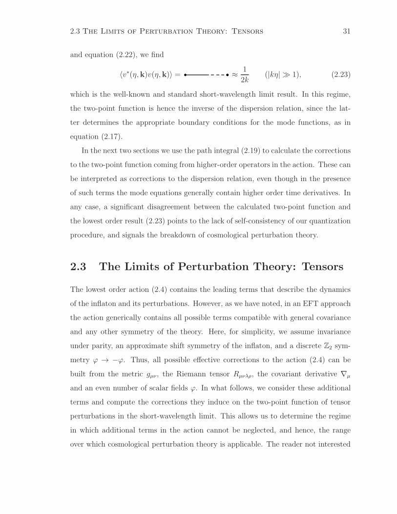
and equation (2.22), we find
〈v∗(η,k)v(η,k)〉 = ≈ 1
2k(|kη| 1), (2.23)
which is the well-known and standard short-wavelength limit result. In this regime,
the two-point function is hence the inverse of the dispersion relation, since the lat-
ter determines the appropriate boundary conditions for the mode functions, as in
equation (2.17).
In the next two sections we use the path integral (2.19) to calculate the corrections
to the two-point function coming from higher-order operators in the action. These can
be interpreted as corrections to the dispersion relation, even though in the presence
of such terms the mode equations generally contain higher order time derivatives. In
any case, a significant disagreement between the calculated two-point function and
the lowest order result (2.23) points to the lack of self-consistency of our quantization
procedure, and signals the breakdown of cosmological perturbation theory.
2.3 The Limits of Perturbation Theory: Tensors
The lowest order action (2.4) contains the leading terms that describe the dynamics
of the inflaton and its perturbations. However, as we have noted, in an EFT approach
the action generically contains all possible terms compatible with general covariance
and any other symmetry of the theory. Here, for simplicity, we assume invariance
under parity, an approximate shift symmetry of the inflaton, and a discrete Z2 sym-
metry ϕ → −ϕ. Thus, all possible effective corrections to the action (2.4) can be
built from the metric gµν , the Riemann tensor Rµνλρ, the covariant derivative ∇µ
and an even number of scalar fields ϕ. In what follows, we consider these additional
terms and compute the corrections they induce on the two-point function of tensor
perturbations in the short-wavelength limit. This allows us to determine the regime
in which additional terms in the action cannot be neglected, and hence, the range
over which cosmological perturbation theory is applicable. The reader not interested
2.3 The Limits of Perturbation Theory: Tensors 32
in technical details may skip directly to section 2.3.3, where we collect and summarize
our results.
2.3.1 Dimension Four Operators
Before tackling the general problem, we begin our analysis by considering the simplest
corrections, namely all dimension four operators, which will appear in the action
multiplied by dimensionless coefficients. On dimensional grounds, we expect these to
yield corrections to the two-point function that are suppressed by only two powers3
of Mp. These operators will also help us to illustrate our formalism and discuss some
of the important issues related to our calculation.
Any generally covariant dimension four effective correction must be of the form
S1 ≡ Sα + Sβ =
∫ √−g(
αR2 + βC2)
, (2.24)
where C2 is the square of the Weyl tensor,
C2 = RµνλρRµνλρ − 2RµνR
µν +1
3R2, (2.25)
and the dimensionless couplings α and β are assumed to be of order one. Note that
we have ignored total derivatives like the Gauss-Bonnet term, since they do not lead
to any corrections in perturbation theory. The Levi-Civita tensor cannot appear in
the action because we assume invariance under parity.
We start by substituting the perturbed metric (2.9) into equation (2.24) and
expanding up to second order in hij. Using the modified background equations and
equation (2.12) to express the tensor perturbations in terms of the variable v, we
3Dimension six operators quadratic in ϕ also contribute at this order; we consider them later.
2.3 The Limits of Perturbation Theory: Tensors 33
obtain in the sub-horizon limit
δ2Sα =α
2M2p
∑
k
∫
dη′
−6a′′
a3vk[
v′′−k + k2v−k]
− 6a′′
a3[
v′′k + k2vk]
v−k
, (2.26)
δ2Sβ =β
M2p
∑
k
∫
dη′
1
a
[
v′′k + k2vk]
− 2 aH(vka
)′
×
1
a
[
v′′−k + k2v−k]
− 2 aH(v−ka
)′
. (2.27)
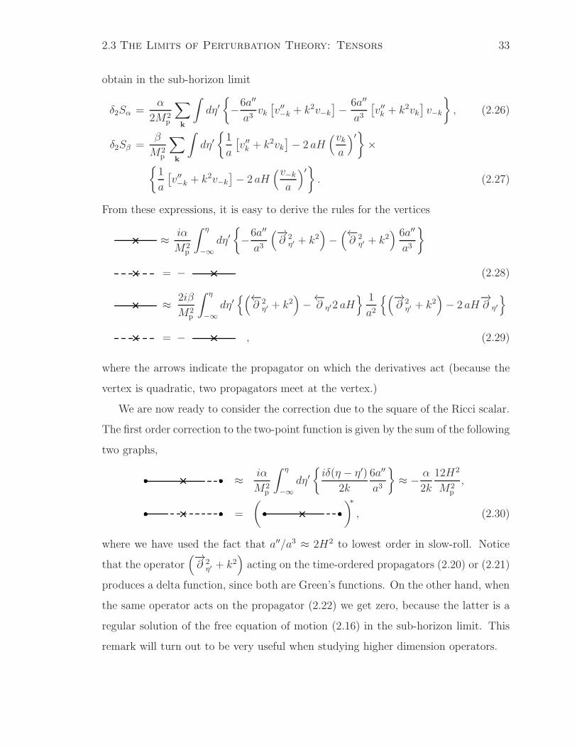
From these expressions, it is easy to derive the rules for the vertices
≈ iα
M2p
∫ η
−∞
dη′
−6a′′
a3
(−→∂ 2η′ + k2
)
−(←−∂ 2η′ + k2
) 6a′′
a3
= − (2.28)
≈ 2iβ
M2p
∫ η
−∞
dη′(←−
∂ 2η′ + k2
)
−←−∂ η′2 aH 1
a2
(−→∂ 2η′ + k2
)
− 2 aH−→∂ η′
= − , (2.29)
where the arrows indicate the propagator on which the derivatives act (because the
vertex is quadratic, two propagators meet at the vertex.)
We are now ready to consider the correction due to the square of the Ricci scalar.
The first order correction to the two-point function is given by the sum of the following
two graphs,
≈ iα
M2p
∫ η
−∞
dη′
iδ(η − η′)2k
6a′′
a3
≈ − α
2k
12H2
M2p
,
=
( )∗
, (2.30)
where we have used the fact that a′′/a3 ≈ 2H2 to lowest order in slow-roll. Notice
that the operator(−→∂ 2η′ + k2
)
acting on the time-ordered propagators (2.20) or (2.21)
produces a delta function, since both are Green’s functions. On the other hand, when
the same operator acts on the propagator (2.22) we get zero, because the latter is a
regular solution of the free equation of motion (2.16) in the sub-horizon limit. This
remark will turn out to be very useful when studying higher dimension operators.
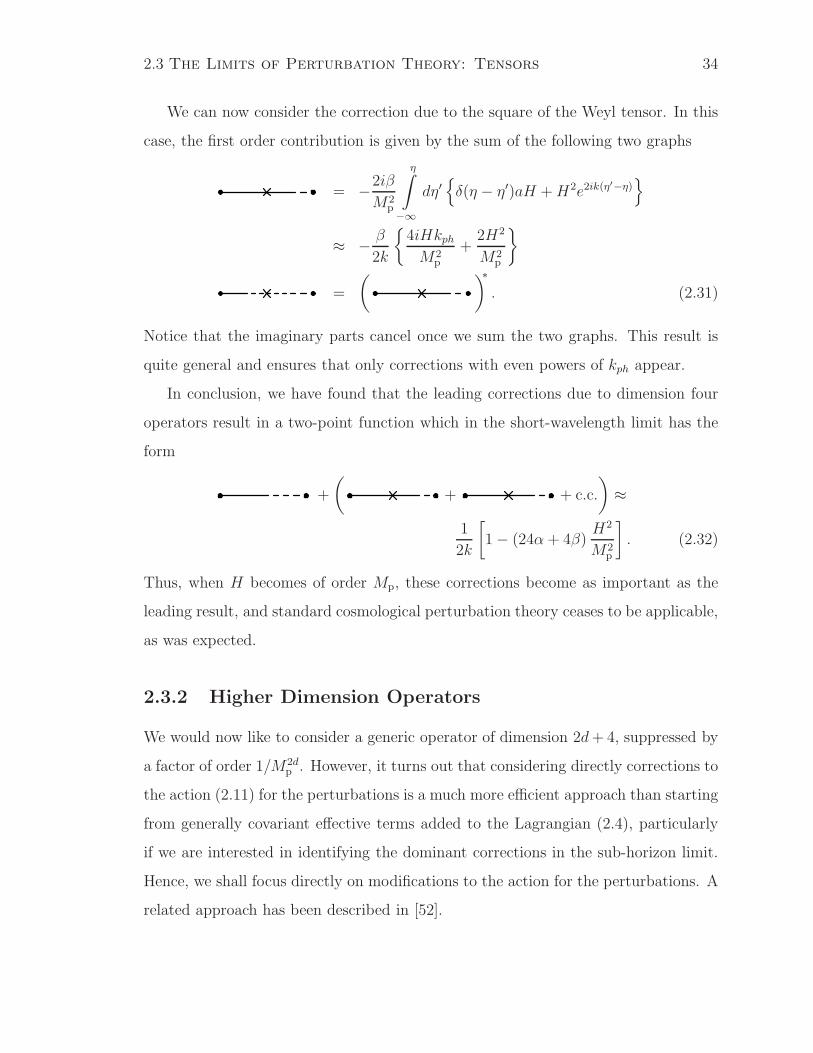
2.3 The Limits of Perturbation Theory: Tensors 34
We can now consider the correction due to the square of the Weyl tensor. In this
case, the first order contribution is given by the sum of the following two graphs
= −2iβ
M2p
η∫
−∞
dη′
δ(η − η′)aH +H2e2ik(η′−η)
≈ − β
2k
4iHkphM2
p
+2H2
M2p
=
( )∗
. (2.31)
Notice that the imaginary parts cancel once we sum the two graphs. This result is
quite general and ensures that only corrections with even powers of kph appear.
In conclusion, we have found that the leading corrections due to dimension four
operators result in a two-point function which in the short-wavelength limit has the
form
+
(
+ + c.c.
)
≈
1
2k
[
1− (24α+ 4β)H2
M2p
]
. (2.32)
Thus, when H becomes of order Mp, these corrections become as important as the
leading result, and standard cosmological perturbation theory ceases to be applicable,
as was expected.
2.3.2 Higher Dimension Operators
We would now like to consider a generic operator of dimension 2d+ 4, suppressed by
a factor of order 1/M2dp . However, it turns out that considering directly corrections to
the action (2.11) for the perturbations is a much more efficient approach than starting
from generally covariant effective terms added to the Lagrangian (2.4), particularly
if we are interested in identifying the dominant corrections in the sub-horizon limit.
Hence, we shall focus directly on modifications to the action for the perturbations. A
related approach has been described in [52].
2.3 The Limits of Perturbation Theory: Tensors 35
Dimensional analysis implies that any operator of dimension 2d + 4, quadratic
in the dimensionless tensor perturbations hij and proportional to 2f powers of the
inflaton field ϕ must contain 2d − 2f + 4 derivatives ∂µ acting on hij , ϕ0(η) and
a(η). The derivatives can be distributed and contracted using the Minkowski metric
in many different ways4, but each of these terms can be schematically represented as
M−2d−2p
(
∂ 2n+m+p [a, ϕ0]) (
∂ 2q+m+r v) (
∂ 2s+p+r v)
, (2.33)
where we have used equation (2.12), and ∂i[a, ϕ0] is just a symbol that represents any
combination of i derivatives acting on a’s and ϕ0’s. One such term would have 2n+
m+p derivatives acting on one or more factors of a or ϕ0, 2q+m+r derivatives acting
on one field v and 2s+p+ r acting on the other v. In particular, 2n of the derivatives
acting on the scale factor or the background field are contracted among themselves
while m and p of them are contracted with derivatives acting on, respectively, the first
and second field v. The derivatives acting on the fields v are organized in a similar
way.
Let us illustrate this notation by considering a term with p = s = f = 0, m =
n = q = 1 and r = 2. Dimensional analysis implies that d = 3, and thus the explicit
form of such a term would be
M−8p ∂ 2+1+0 [a] ∂ 2+1+2 v ∂ 0+0+2 v =M−8
p ∂µ∂µ ∂ν [a] ∂λ∂
λ ∂ν ∂α∂β v ∂α∂β v , (2.34)
where ∂µ∂µ∂ν [a] denotes all possible ways to construct a term with three derivatives
of the scale factor, with the given tensor structure.
4The reader may think that derivatives could be contracted not only among each other with
the Minkowski metric, but also by using the additional tensor structure provided by the metric
perturbations δgµν/a2 = hijηµiηνj . However, it turns out that
(
δgµν/a2)
∂νa = hijηµi∂ja = 0 and,
since hij is transverse,
∂µ(
δgµν/a2)
= ηνj∂ihij = 0 .
Thus, we get a non-vanishing contribution only when we contract derivatives with the Minkowski
metric while the factors ηµiηνj are contracted among each other yielding an irrelevant overall factor.
2.3 The Limits of Perturbation Theory: Tensors 36
The first step to estimate the leading correction due to a term of the form (2.33)
is realizing that this can always be expressed as a linear combination of terms of the
form
M−2d−2p ∂2j+l [a, ϕ0] ∂
2m+lv ∂µ∂µv, (2.35)
plus, possibly, a term with no derivatives acting on v, which in any case gives a
contribution that is always subdominant in the sub-horizon limit. A proof of this
goes as follows. We want to integrate by parts every term of the form
∂ 2n+m+p [a, ϕ0] ∂2q+m+r v ∂ 2s+p+r v (2.36)
in order to express it as a linear combination of terms like
∂2j+l [a, ϕ0] ∂2m+lv v (2.37)
plus, possibly, a term with no derivatives acting on v. Notice that, for notational
convenience, we have defined ≡ ∂µ∂µ. Of course, if the index q (or s) in equa-
tion (2.36) is not zero, we can easily integrate by parts 2q+m+ r−2 (2s+ p+ r−2)
times to get only terms of the form of that in equation (2.37). Therefore, in what
follows we only consider terms with q = s = 0. When this is the case, we can always
integrate by parts an appropriate number of times to get only terms for which m = p.
Thus, without loss of generality, we can restrict ourselves to considering terms of the
form
∂ 2n+m+p [a, ϕ0] ∂m+r v ∂ p+r v, (m = p) . (2.38)
The derivatives acting on v that are contracted with derivatives acting on a or ϕ0 can
be systematically eliminated by repeated integrations by parts:
∂ 2n+m+p [a, ϕ0] ∂m+r v ∂ p+r v ∼ −∂ 2n+m+(p−1) [a, ϕ0] ∂
m+r v ∂ (p−1)+r v (2.39)
+1
2∂ 2(n+1)+(m−1)+(p−1) [a, ϕ0] ∂
(m−1)+(r+1) v ∂ (p−1)+(r+1) v ,
where we have denoted equivalence up to integration by parts with ∼. The first termon the right hand side can be cast in the form (2.37) by integrating by parts (p−1)+r

2.3 The Limits of Perturbation Theory: Tensors 37
times, while the second one is of the form (2.38) with n and r (p and m) increased
(decreased) by one. By iterating this procedure, we eventually obtain terms of the
form
∂ 2n [a, ϕ0] ∂r v ∂ r v , (2.40)
where now n and r have changed. Again, we can integrate by parts and obtain
∂ 2n [a, ϕ0] ∂r v ∂ r v ∼ −∂ 2n [a, ϕ0] ∂
r−1 v ∂ r−1 v +1
2∂ 2(n+1) [a, ϕ0] ∂
(r−1) v ∂ (r−1) v .
The first term on the right hand side can be re-written as (2.37) after r−1 integrationsby parts, while the second term has the form (2.40) with n (r) increased (decreased)
by one. Thus, by repeating this procedure we obtain many terms of the form (2.37)
and we are eventually left with a term without derivatives acting on v. This completes
our proof. In what follows, we therefore restrict ourselves to terms of the form (2.35).
Dimensional analysis requires that the indexes j, l and m in equation (2.35) obey
j + l +m = d− f + 1 . (2.41)
Furthermore, since dnϕ0/dηn ∝√2εMp a
nHn and dna/dηn ∝ an+1Hn, each field ϕ0
yields a factor of Mp, while each derivative acting on it or on the scale factor results
in a factor of H to leading order in slow-roll. Finally, the l partial derivatives ∂µ
acting on v that are contracted with derivatives acting on a or ϕ0 can be turned into
derivatives with respect to η only. Thus, (2.35) can be re-written as
M−2d+2f−2p f(a)H2j+lm∂ lηv v , (2.42)
where we have defined ≡ ∂µ∂µ; the corresponding correction to the two-point
function is schematically given by
=i
M2d−2f+2p
∫ η
−∞
dη′f(a)H2j+l × (2.43)
(←−m←−∂ l
η′−→ +
←−−→∂ lη′−→m)
2.3 The Limits of Perturbation Theory: Tensors 38
plus the complex conjugate of this graph. Because (2.22) satisfies the free equation
of motion, this correction is non-vanishing only when the index m is equal to zero,
and in this case we obtain
=1
M2d−2f+2p
η∫
−∞
dη′f(a)H2j+lδ(η − η′)(ik)l
2k
=f(a)
2k
H2j+l(ik)l
M2d−2f+2p
. (2.44)
The leading correction in the short-wavelength limit is the one with the maximum
number of powers of k. According to equation (2.41), this maximum number simply
equals d − f + 1 ≡ lmax, and it corresponds to the case in which j = m = 0.
Thus, if d− f is odd, lmax is even and the leading correction is simply given by
δ〈v∗(k)v(k)〉 ∝ 1
2k
(
H
Mp
)d−f+1 (kphMp
)d−f+1
(d− f odd) , (2.45)
since each factor of k/Mp must be accompanied by a factor of a to render the spatial
momentum physical. On the other hand, if d−f is even, lmax as defined above is odd
and the term with the highest number of powers of k is purely imaginary. As we have
seen in the previous section, such a term disappears when we add the contribution
from the complex conjugate graph. Therefore, the leading correction corresponds to
the largest even value of l, which turns out to be lmax = d− f , and is therefore given
by
δ〈v∗(k)v(k)〉 ∝ 1
2k
(
H
Mp
)d−f+2 (kphMp
)d−f
(d− f even) . (2.46)
Equations (2.45) and (2.46) represent the main results of this section: they express
the leading corrections to the two-point function (in the sub-horizon limit) associated
with a generic operator of dimension 2d+4 containing 2f powers of the inflaton field.
Since we have assumed an approximate shift invariance of the inflaton, the total
number of derivatives, 2d−2f+2, must be greater or equal than the number of fields
2f , which in turn implies that d ≥ f . Thus, we can label all the possible corrections
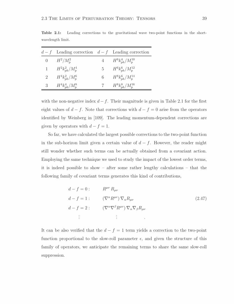
2.3 The Limits of Perturbation Theory: Tensors 39
Table 2.1: Leading corrections to the gravitational wave two-point functions in the short-
wavelength limit.
d− f Leading correction d− f Leading correction
0 H2/M2p 4 H6k4ph/M
10p
1 H2k2ph/M4p 5 H6k6ph/M
12p
2 H4k2ph/M6p 6 H8k6ph/M
14p
3 H4k4ph/M8p 7 H8k8ph/M
16p
with the non-negative index d− f . Their magnitude is given in Table 2.1 for the first
eight values of d − f . Note that corrections with d− f = 0 arise from the operators
identified by Weinberg in [109]. The leading momentum-dependent corrections are
given by operators with d− f = 1.
So far, we have calculated the largest possible corrections to the two-point function
in the sub-horizon limit given a certain value of d − f . However, the reader might
still wonder whether such terms can be actually obtained from a covariant action.
Employing the same technique we used to study the impact of the lowest order terms,
it is indeed possible to show – after some rather lengthy calculations – that the
following family of covariant terms generates this kind of contributions,
d− f = 0 : Rµν Rµν
d− f = 1 : (∇αRµν)∇αRµν (2.47)
d− f = 2 : (∇α∇βRµν)∇α∇βRµν
...... .
It can be also verified that the d − f = 1 term yields a correction to the two-point
function proportional to the slow-roll parameter ε, and given the structure of this
family of operators, we anticipate the remaining terms to share the same slow-roll
suppression.

2.3 The Limits of Perturbation Theory: Tensors 40
2.3.3 The Three-Momentum Scale Λ
The corrections to the two-point function are functions of two dimensionful param-
eters, H and kph. For our purposes, it is convenient to organize these corrections in
powers of kph. Thus, following Table 2.1, and reintroducing the subleading terms that
we previously neglected, we find that the two-point function is
〈v∗(k)v(k)〉 ≈ 1
2k
[
(
1 + α20H2
M2p
+ · · ·)
+
(
α22H2
M2p
+ α42H4
M4p
+ · · ·)
k2phM2
p
+
+
(
α44H4
M4p
+ α64H6
M6p
+ · · ·)
k4phM4
p
+ · · ·]
. (2.48)
The coefficient α20 is of order one, while all the αnn with n ≥ 2 are of order ε, as
the family of covariant terms (2.48) suggests. At the end of Section 2.4 we provide
further evidence supporting this claim.
In order for Equation (2.48) to be a valid perturbative expansion, every correction
term must be much smaller than one. Because α20 is of order one, this implies the
conditionH
Mp 1, (2.49)
which must hold for all values of kph. Equation (2.48) then shows that if condition
(2.49) is satisfied, the corrections to the two-point function remain small even for
kph ≈Mp. In fact, to leading order in H/Mp we can rewrite equation (2.48) as
〈v∗(k)v(k)〉 ≈ 1
2k
[
1 + α22
k2phΛ2
+ α44
k4phΛ4
+ · · ·]
, (2.50)
where we have introduced the effective cutoff
Λ ≈M2
p
H. (2.51)
Equations (2.50) and (2.51) are the main result we were aiming at, given that
they show the three-momentum scale at which the perturbative expansion fails. For
kph Λ, all the corrections are strongly suppressed and can thus be neglected.
However, at kph ≈ Λ, all the corrections become of the same order ε, the asymptotic
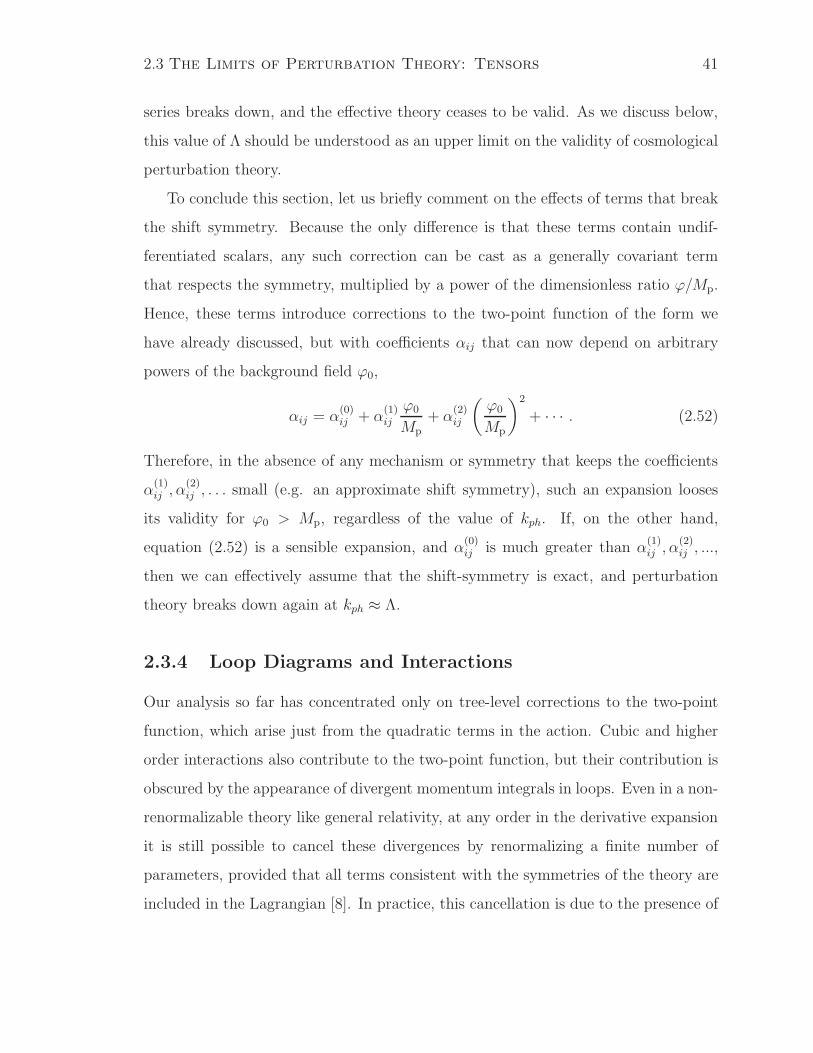
2.3 The Limits of Perturbation Theory: Tensors 41
series breaks down, and the effective theory ceases to be valid. As we discuss below,
this value of Λ should be understood as an upper limit on the validity of cosmological
perturbation theory.
To conclude this section, let us briefly comment on the effects of terms that break
the shift symmetry. Because the only difference is that these terms contain undif-
ferentiated scalars, any such correction can be cast as a generally covariant term
that respects the symmetry, multiplied by a power of the dimensionless ratio ϕ/Mp.
Hence, these terms introduce corrections to the two-point function of the form we
have already discussed, but with coefficients αij that can now depend on arbitrary
powers of the background field ϕ0,
αij = α(0)ij + α
(1)ij
ϕ0
Mp
+ α(2)ij
(
ϕ0
Mp
)2
+ · · · . (2.52)
Therefore, in the absence of any mechanism or symmetry that keeps the coefficients
α(1)ij , α
(2)ij , . . . small (e.g. an approximate shift symmetry), such an expansion looses
its validity for ϕ0 > Mp, regardless of the value of kph. If, on the other hand,
equation (2.52) is a sensible expansion, and α(0)ij is much greater than α
(1)ij , α
(2)ij , ...,
then we can effectively assume that the shift-symmetry is exact, and perturbation
theory breaks down again at kph ≈ Λ.
2.3.4 Loop Diagrams and Interactions
Our analysis so far has concentrated only on tree-level corrections to the two-point
function, which arise just from the quadratic terms in the action. Cubic and higher
order interactions also contribute to the two-point function, but their contribution is
obscured by the appearance of divergent momentum integrals in loops. Even in a non-
renormalizable theory like general relativity, at any order in the derivative expansion
it is still possible to cancel these divergences by renormalizing a finite number of
parameters, provided that all terms consistent with the symmetries of the theory are
included in the Lagrangian [8]. In practice, this cancellation is due to the presence of
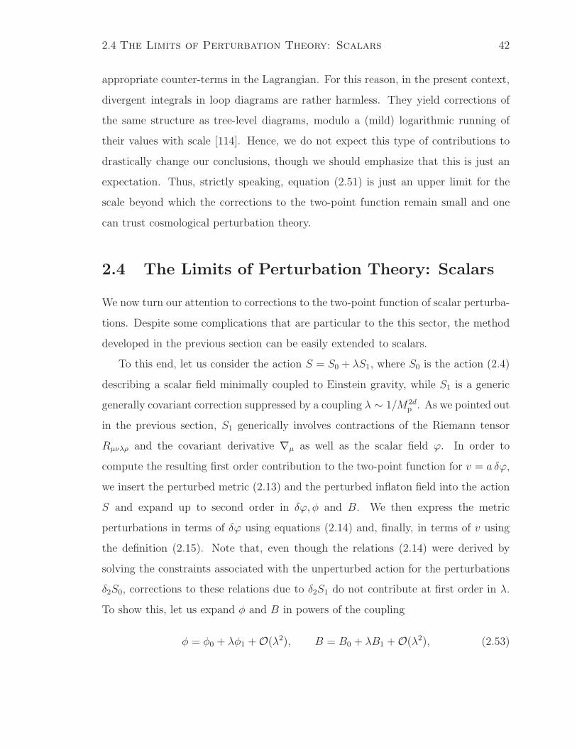
2.4 The Limits of Perturbation Theory: Scalars 42
appropriate counter-terms in the Lagrangian. For this reason, in the present context,
divergent integrals in loop diagrams are rather harmless. They yield corrections of
the same structure as tree-level diagrams, modulo a (mild) logarithmic running of
their values with scale [114]. Hence, we do not expect this type of contributions to
drastically change our conclusions, though we should emphasize that this is just an
expectation. Thus, strictly speaking, equation (2.51) is just an upper limit for the
scale beyond which the corrections to the two-point function remain small and one
can trust cosmological perturbation theory.
2.4 The Limits of Perturbation Theory: Scalars
We now turn our attention to corrections to the two-point function of scalar perturba-
tions. Despite some complications that are particular to the this sector, the method
developed in the previous section can be easily extended to scalars.
To this end, let us consider the action S = S0 + λS1, where S0 is the action (2.4)
describing a scalar field minimally coupled to Einstein gravity, while S1 is a generic
generally covariant correction suppressed by a coupling λ ∼ 1/M2dp . As we pointed out
in the previous section, S1 generically involves contractions of the Riemann tensor
Rµνλρ and the covariant derivative ∇µ as well as the scalar field ϕ. In order to
compute the resulting first order contribution to the two-point function for v = a δϕ,
we insert the perturbed metric (2.13) and the perturbed inflaton field into the action
S and expand up to second order in δϕ, φ and B. We then express the metric
perturbations in terms of δϕ using equations (2.14) and, finally, in terms of v using
the definition (2.15). Note that, even though the relations (2.14) were derived by
solving the constraints associated with the unperturbed action for the perturbations
δ2S0, corrections to these relations due to δ2S1 do not contribute at first order in λ.
To show this, let us expand φ and B in powers of the coupling
φ = φ0 + λφ1 +O(λ2), B = B0 + λB1 +O(λ2), (2.53)

2.4 The Limits of Perturbation Theory: Scalars 43
where φ0 and B0 satisfy the unperturbed relations (2.14) and (2.14) respectively. By
expanding the full quadratic action for the perturbations δ2S [δϕ, φ, B] to first order
in λ we obtain
δ2S [δϕ, φ, B] ≈ δ2S0 [δϕ, φ0, B0] + λ
∫[
δ(δ2S0)
δφ
]
λ=0
φ1 + λ
∫[
δ(δ2S0)
δB
]
λ=0
B1
+λ δ2S1[δϕ, φ0, B0] +O(λ2). (2.54)
However, the second and the third term vanish because they contain the unperturbed
constraint equations evaluated at φ0 and B0, which by assumption are solutions to
the constraints. Therefore, as long as we are interested in first order results, we can
safely use the unperturbed solutions φ0 and B0 given by equations (2.14).
Expanding the leading action S0 to quadratic order in the perturbations, we obtain
the free action (2.11). The additional quadratic terms stemming from S1 must be
appropriately contracted expressions containing partial derivatives of the perturbation
variable v, the scale factor a and the background field ϕ0. However, in the case
of scalar perturbations, the field v can arise from fluctuations of the scalar field,
δϕ = v/a, or from fluctuations of the metric,
δgµν = −a√2ε
Mp
[
2vkδµ0δν0 +
ikjk2
(v′k − aHvk) (δµjδν0 + δµ0δνj)
]
≡ a√2εVµνMp
.
(2.55)
Thus, unlike the case of tensor perturbations, δgµν provides an additional tensor
structure that can be used to contract derivatives. We now show that such contrac-
tions yield terms where the derivatives acting on v or a are contracted with ηµν . This
means that the argument in the previous section can be applied to scalar perturba-
tions as well, yielding essentially the same results. We note that terms which contain
only fluctuations coming directly from the scalar field do not present this problem,
and can be easily written as in equation (2.33).
Let us first consider terms with only one factor of Vµν . In this case, Vµν can be
contracted either with ηµν , leading to Vµνηµν = 2 v, or with two derivatives ∂µ∂ν ,
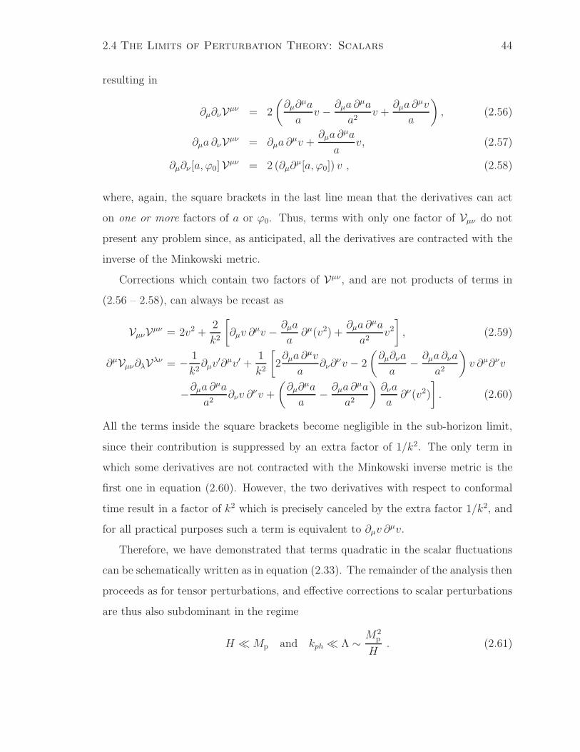
2.4 The Limits of Perturbation Theory: Scalars 44
resulting in
∂µ∂νVµν = 2
(
∂µ∂µa
av − ∂µa ∂
µa
a2v +
∂µa ∂µv
a
)
, (2.56)
∂µa ∂νVµν = ∂µa ∂µv +
∂µa ∂µa
av, (2.57)
∂µ∂ν [a, ϕ0]Vµν = 2 (∂µ∂µ[a, ϕ0]) v , (2.58)
where, again, the square brackets in the last line mean that the derivatives can act
on one or more factors of a or ϕ0. Thus, terms with only one factor of Vµν do not
present any problem since, as anticipated, all the derivatives are contracted with the
inverse of the Minkowski metric.
Corrections which contain two factors of Vµν , and are not products of terms in
(2.56 – 2.58), can always be recast as
VµνVµν = 2v2 +2
k2
[
∂µv ∂µv − ∂µa
a∂µ(v2) +
∂µa ∂µa
a2v2]
, (2.59)
∂µVµν∂λVλν = − 1
k2∂µv
′∂µv′ +1
k2
[
2∂µa ∂
µv
a∂ν∂
νv − 2
(
∂µ∂νa
a− ∂µa ∂νa
a2
)
v ∂µ∂νv
−∂µa ∂µa
a2∂νv ∂
νv +
(
∂µ∂µa
a− ∂µa ∂
µa
a2
)
∂νa
a∂ν(v2)
]
. (2.60)
All the terms inside the square brackets become negligible in the sub-horizon limit,
since their contribution is suppressed by an extra factor of 1/k2. The only term in
which some derivatives are not contracted with the Minkowski inverse metric is the
first one in equation (2.60). However, the two derivatives with respect to conformal
time result in a factor of k2 which is precisely canceled by the extra factor 1/k2, and
for all practical purposes such a term is equivalent to ∂µv ∂µv.
Therefore, we have demonstrated that terms quadratic in the scalar fluctuations
can be schematically written as in equation (2.33). The remainder of the analysis then
proceeds as for tensor perturbations, and effective corrections to scalar perturbations
are thus also subdominant in the regime
H Mp and kph Λ ∼M2
p
H. (2.61)
2.5 Discussion 45
Before concluding, we would like to address again whether the operators that
we have considered can be actually obtained from generally covariant terms. In
the case of scalar perturbations, it is indeed possible to show – after further rather
lengthy calculations – that the following family of covariant terms generates the kind
of corrections shown in Table 2.1,
d− f = 0 : Rµν (∇µ ϕ)∇ν ϕ
d− f = 1 : Rµν (∇µ ϕ)∇ν∇γ∇γ ϕ (2.62)
d− f = 2 : (∇α∇βRµν) (∇α∇µ ϕ)∇β∇ν ϕ
d− f = 3 : (∇α∇βRµν) (∇α∇µ ϕ)∇β∇ν∇γ∇γ ϕ
...... .
In order to illustrate how this happens, let us consider for example the d − f = 1
term. It contains, among many other terms a factor
a2Rµν ∂µ δϕ ∂ν ∂γ ∂γ δϕ ⊃ 2ε
a6∂µa ∂νa ∂µ v ∂ν ∂γ ∂
γ v ∼ −2ε
a6∂µa ∂νa ∂µ ∂ν v v + ...
(2.63)
where, in the last step, we have neglected a subdominant contribution in the short-
wavelength limit. The last term in (2.63) indeed generates a correction proportional to
H2k2ph/M4p and it is suppressed by one factor of the slow-roll parameter. It is relatively
easy to verify that the corrections generated by the other members of the family (2.62)
have the same slow-roll suppression, which strongly supports the assumption we made
in the context of tensor perturbations.
2.5 Discussion
The connection, through cosmological inflation, between physics on the smallest
scales, described by quantum field theory, and that on the largest scales in the uni-
verse is one of the most profound aspects of modern cosmology. However, since
inflation takes place at such early epochs, and magnifies fluctuations of such small
2.5 Discussion 46
wavelengths, it is important to establish the regime of validity of the usual formalism
– that of semiclassical gravity, with quantum field theory assumed valid, and coupled
to the minimal Einstein-Hilbert action – at those scales.
On general grounds, we expect the canonical approach to break down at ultra-
short distances, where the operators that arise in an EFT treatment of the coupled
metric-inflaton system become relevant. In this chapter we have calculated the impact
of these higher-dimensional operators on the power spectrum at short wavelengths.
In this way, we have been able to probe the regime in which the properties of the
perturbations deviate from what is conventionally assumed. From a purely theoretical
standpoint, these considerations are important if we are to understand the limits of
applicability of cosmological perturbation theory. From an observational standpoint,
cosmic microwave background measurements are becoming so precise that we may
hope to use them to identify the signatures of new gravitational or field theoretic
physics.
Our analysis has focused on tree-level corrections to the spectrum. Because we
have essentially considered all possible generally covariant terms in the effective ac-
tion, we expect to have unveiled the form of all possible corrections that are compat-
ible with the underlying symmetries of the theory. It is however possible that loop
diagrams yield additional corrections that we have not considered. In any case, our
results indicate that cosmological perturbation theory does not apply all the way to
infinitesimally small distances, kph →∞, and that, indeed, there is a physical spatial
momentum Λ (or a physical length 1/Λ) beyond which cosmological perturbation
ceases to be valid. The scale at which perturbation theory breaks down has to be
lower than
Λ ∼M2
p
H, (2.64)
which, because of existing limits on the scalar to tensor power spectrum ratio [115],
is at least 104 times the Planck scale.
These results have significant implications for the impact of trans-Planckian physics

2.5 Discussion 47
on the primordial spectrum of primordial perturbations, which typically is at most
of order H/Λ [95]. Substituting the upper limit of Λ we have found, we obtain cor-
rections of the order of H2/M2p , which are likely to remain unobservable [99]. This
value of Λ also solves a problem that was noticed in [116], namely, that in the pres-
ence of a Planckian cutoff, cosmological perturbations do not tend to decay into the
Bunch-Davis vacuum (or similar states). In particular, to lowest order in perturba-
tion theory, the transition probability from an excited state into the Bunch-Davis
vacuum is significantly less than one for Λ = Mp, but proportionally larger if Λ is
given by (2.64). Ultimately, a large decay probability is what justifies the choice of
the Bunch-Davies vacuum as the preferred initial state for the perturbations at scales
below the cutoff, since, as we have found, our theories certainly lose their validity at
momentum scales above the spatial momentum Λ.

Chapter 3
Eucidean Path Integral Formalism
and 6th Order Corrections
3.1 Introduction
We have seen in the previous chapter how the effective field theory approach can be
applied to problems such as determining the limits of validity of perturbation theory
in the early universe. We can now take a more radical point of view, still looking for
small corrections of the underlying cosmological system (here the description of late
time acceleration), but now giving physical meaning to some higher derivative terms
via the Euclidean path integral formulation.
One of the main motivation for considering higher order systems comes from fairly
recent developments in modeling late time acceleration. The suggestion that the ac-
celerated expansion of the universe may be explained by an infrared modification
of gravity has fueled renewed interest in higher derivative theories and their associ-
ated pathologies [117–124]. Corrections to the Einstein-Hilbert action, when coming
from pure gravity, must be constructed with covariant contractions of powers of the
Riemann tensor. When this happens though, the corrections may contain four or
more time derivatives acting on the physical field, the metric. We have seen in the

3.1 Introduction 49
introduction in section 1.3.1 that, a few special cases aside, systems with more than
two time derivatives can be described via a classically equivalent Lagrangian that
quite generically contains ghosts – degrees of freedom with the wrong sign for the
kinetic term. These ghosts lead to catastrophic instabilities if they appear in the
perturbative spectrum and hence have to be removed or “cured”. It follows then that
unless a scheme to deal with the ghosts is chosen, the models containing them become
unsuitable to describe physical phenomena.
The best known and standard way to make sense of theories with higher derivatives
is through the effective field theory approach described and utilized in the previous
chapters. We recall that, from the EFT point of view, terms that contain higher
derivatives appear from an expansion of an unknown UV-complete theory. This
expansion, by definition, is supposed to provide an accurate description of the full
theory only at low energies, and the physical degrees of freedom are assumed to be
only those that appear in the ground state of the theory [52]. Classically, the presence
of extra solutions to the field equations that correspond to the existence of ghosts is
then considered as an artifact of the effective theory, due to the truncation of an
infinite series. If then, for instance, it is possible to push the masses of these degrees
of freedom beyond the cutoff – the energy scale below which the effective field theory
is trusted – the ghosts can be ignored.
Effective field theory then provides a safe way to deal with higher derivatives. They
arise naturally and are considered an artifact, so can be ignored unless they introduce
unwanted corrections below the cutoff. This is the point of view taken in chapter 2,
where back-substitution has been enforced. In other words, in the previous chapter
the propagators were defined by the quadratic free action, and so only described the
propagation of the degrees of freedom of the low energy second order theory. At
the same time, higher time derivatives have been treated as interactions – vertices –
correcting the propagation of the physical degrees of freedom.
The story seems to be complete, and there seems to be very little need to go beyond

3.1 Introduction 50
these ideas, especially since difficulties like ghost fields lurk around the corner. This
is of course, unless one thinks that higher derivative terms in the action may have
a physical meaning. We cite here a couple of these alternative procedures that have
been proposed to deal with higher derivative terms [125, 126]. In these works the
authors apply new procedures to usual systems finding results that differ from the
canonical EFT treatment, and that have quite deep philosophical consequences. In
the first case for instance, it is shown that quantum systems described by a higher
derivative action may not have a classical smooth limit (in their description), while
retaining the ability of matching observational constraints. In the second case instead,
the main purpose is to try to get closer to a quantizable and renormalizable theory
of gravity.
Quite in general, taking the bottom-up approach from GR to a more funda-
mental theory of quantum gravity, higher derivatives appear and going beyond the
parametrization of our ignorance of such a theory requires making physical sense of
these objects.
We can then see that there are very good motivations to think of higher order
terms, and also to look for something else than EFT. In fact it has to be said that
EFT, relying on a series expansion also lacks the ability of describing runaway solu-
tions which in general are troublesome, but that may make sense in a cosmological
framework [61].
In this chapter we will focus on the prescription introduced by Hawking and
Hertog [126], who demonstrated that the Euclidean path integral formulation of the
quantum theory allows one to define a probability distribution for a scalar field that
appears in the Lagrangian with four time derivatives. In particular their work tried to
make sense of the ghosts without incorporating them into the full physical theory, but
by assuming that they correspond to some infinities that – like in many other theories
– need to be integrated away in some smart way to avoid losing the information they
hide. Adopting this point of view, the Euclidean path integral approach could be
3.1 Introduction 51
seen as a substitute of EFT and nothing more, since its main purpose is still to find
corrections to the lower order theory. Either way an interesting result arises; in fact
the two methods do not always agree allowing for a possibility of testing their efficacy
and validity with experiments, and therefore moving from speculation to physics.
It will be more clear later, when the details of the calculations are shown, that if the
higher order terms are considered as corrections to the second order action for the field,
the results calculated in the Euclidean path integral approach could lead, in principle,
to a different physical result. This happens because corrections to the probability for
the fields may display a different dependence on the “coupling constant” than the
equivalent corrections calculated via EFT. Here by “coupling constant” we mean the
parameter that controls the strength of the higher order term in the action. For
example, in higher order theories of gravity here considered, the “coupling constant”
contains appropriate inverse powers of the cutoff scale. A different dependence on the
behavior of such corrections may shift the energy at which they become important.
However, at fourth order, the analysis in [127] of a term proportional to the Weyl
tensor squared demonstrated that in a de Sitter background there is no discrepancy
between the Euclidean path integral procedure and the effective field theory one.
In this chapter, we explore further whether the Euclidean path integral approach
can be extended to apply generally, to higher derivative orders, and study whether
observational differences from the effective field theory approach can be realized in
practice. Since the study of a general higher derivative correction to the Einstein-
Hilbert action is prohibitively complicated, we therefore focus here on a nontrivial
correction beyond 4th order, namely the 6th order term ∇αRµν∇αRµν . As we will
see, this is sufficient to draw interesting conclusions. We demonstrate how to apply,
at least in principle, the Euclidean path integral prescription to sixth order terms.
However, the question of whether it can be applied to a specific system such as
General Relativity plus fourth and sixth order corrections is highly dependent on the
choice of background. In particular, a Minkowski background always admits choices

3.2 Review of the Hawking-Hertog Formalism 52
for the “coupling constants” that yield a well defined Euclidean theory. On the other
hand a de Sitter background, due to its explicit time dependence, introduces some
complications, since the simple requirements to apply the whole prescription are not
met. Nevertheless, as happened in the fourth order case, we shall see that this does
not preclude the possibility of finding a viable result.
The chapter is organized as follows. Section 3.2 is devoted to a brief review of the
Euclidean path integral approach, and a discussion of its generalization to sixth order
for a certain class of quadratic Lagrangians. In section 3.3 we derive the perturbed
action for tensorial modes coming from a sixth order action about two backgrounds,
Minkowski and de Sitter. We then solve for the classical solutions and perform the
canonical procedure to build the path integral in the Lagrangian formulation. Finally,
in section 3.4 we comment on the results and present our conclusions. As done
before, we use t and η to denote cosmological and conformal times respectively, and
denote the time derivative with respect to them with an overdot d/dt ≡ ˙( ), with the
difference between t and η being clear from the context. After a Wick rotation the
time coordinate is described by a real parameter that for both cosmic and conformal
times we call τ , and the derivative with respect to it is represented by a prime sign
d/dτ ≡ ( )′. Conformal time is only used when the de Sitter background is taken into
consideration.
3.2 Review of the Hawking-Hertog Formalism
We can start by reviewing the idea behind the Euclidean path integral procedure and
discussing the ways in which the fourth order case differs from the usual second order
treatment.
Following the lines of what we have seen in the introduction in sections 1.2, 1.3.1,
and 1.3.2, in a second order theory the propagator for a field φ defined by a Lagrangian
3.2 Review of the Hawking-Hertog Formalism 53
Lφ can be found computing a path integral between the initial and final configurations
〈(φf ; tf)|(φi; ti)〉 =∫ φf
φi
d[φ(t)] exp [iS[φ]] , (3.1)
where the action for the field is given by
S[φ] =
∫ tf
ti
dt′L(φ, φ, t′) . (3.2)
Here φ× represents the state of the field at time t×. A system described by a quadratic
Lagrangian with a higher number of time derivatives can be transformed into a second
order system via nonlinear transformations1; for instance a fourth order system with
Lagrangian
L = −12φ
(
d2
dt2−m2
1
)(
d2
dt2−m2
2
)
φ, (3.3)
can be recast as
L =1
2ψ1
(
d2
dt2−m2
1
)
ψ1 −1
2ψ2
(
d2
dt2−m2
2
)
ψ2 , (3.4)
where ψ1 and ψ2 are defined via
ψ1 =( d
2
dt2−m2
2)φ√
m22 −m2
1
, ψ2 =( d
2
dt2−m2
1)φ√
m22 −m2
1
. (3.5)
In the canonical treatment of higher order systems, this transformed Lagrangian (3.4)
is the starting point and the system is viewed as a multi-field one, where at least one
of the newly defined second order fields is a ghost. In the case at hand it is easy to
note that ψ1 has the wrong sign for the kinetic term, playing the role of the ghost
field.
The propagator is given by a path integral over both fields
〈(ψ2f , ψ1f ; tf)|(ψ2iψ1i; ti)〉 =∫ (ψ2,ψ1)f
(ψ2,ψ1)i
d[ψ2(t)]d[ψ1(t)] exp [iS[ψ2, ψ1]] . (3.6)
Note that via the definitions of ψ1 and ψ2, this functional integration can be inter-
preted as integrating over the original field φ and its second time derivative. However,
1We can ignore spatial dependence for the moment or, equivalently, we think of the field φ as a
particular Fourier mode.

3.2 Review of the Hawking-Hertog Formalism 54
as pointed out in [126], this choice presents a problem. For second order systems the
propagator obeys the composition law
G(φ3, φ1) =
∫
d[φ2]G(φ3, φ2)G(φ2, φ1) , (3.7)
where G(φ3, φ1) is the propagator between the two states “1” and “3”, and “2”
represents an intermediate state. When one joins the fields above and below the
intermediate time t2, the value of the field φ(t2) is fixed, but its time derivative is
not, resulting in a jump in φ(t2), which in turn corresponds to a delta function in the
value of φ(t2). Unfortunately, in the original fourth order action (3.3) the second time
derivative appears quadratically, and hence the original composition law of the path
integral is lost and infinities arise. This argument applies quite generally to higher
derivative systems as we have seen in section 1.3.1.
In contrast to using the two new fields that are combinations of the original
field and its second derivative, the alternative procedure proposed in [126] to deal
with fourth order systems requires the fundamental variables to be the field and its
first time derivative. This choice is motivated by the need to retain the continuity
properties of the path integral formulation, as described above2. However, this point
of view introduces a different problem; initial and final states are then described in
terms of φ and φ, which behave much like position and momentum for a particle
in quantum mechanics. The proposed procedure consists into rotating the system
to Euclidean time, and then integrating out the φ dependence in the definition of
probabilities, thus obtaining well defined quantum mechanical observables at the price
of a loss of unitarity. This procedure has always been possible in the special cases
studied in the literature so far.
We can give a summary of the practical procedure that schematically reads:
1. From the fourth order action S perform a Wick rotation to obtain the Euclidean
action SE,
2We refer to the original article [126] for a longer discussion that would distract us here from the
main point.
3.2 Review of the Hawking-Hertog Formalism 55
2. Derive the Euclidean equations of motion and corresponding solutions,
3. Use the Euclidean version of the path integral to find the propagator for φ with
boundary conditions on φ and φ′,
4. Define a “wavefunctional” as the propagator from a vacuum state at minus
infinity in Euclidean time,
5. Find the modulus squared of the wavefunctional, or probability amplitude,
which gives the probability that a quantum fluctuation leads to a state with
specified φ and φ′,
6. Finally, and crucially, trace over φ′ before returning to real time. Note that if
one were to rotate back to Lorentzian time before integrating, the probability
would be ill defined, reflecting the existence of the ghost degree of freedom.
There is no magic trick behind all this, since taming the ghost by integrating over
the infinities that it introduces happens at the price of a violation of unitarity3. The
Euclidean formulation of the path integral together with the requirement that the
fields die off at Euclidean infinity ensures that the fields remain bounded in real time.
This is similar to using a final boundary condition to remove runaway solutions from
systems that would otherwise contain them.
Let us examine this procedure in the specific case of the 4th order system discussed
earlier. Using t for Lorentzian and τ for Euclidean time, rescaling the field φ, the
action is
S =
∫
dt
(
α2
2φ2 − 1
2φ2 +
m2
2φ2
)
, (3.8)
where α2/2 is an arbitrary small parameter, the “coupling constant” mentioned ear-
lier. After a Wick rotation t→ iτ the action becomes
SE ≡∫
dτ
(
α2
2φ′′2 +
1
2φ′2 +
m2
2φ2
)
, (3.9)
3The interested reader can refer to the original paper [126] for a detailed discussion of this issue.
3.2 Review of the Hawking-Hertog Formalism 56
so that iS → −SE in the path integral. When SE is positive definite the path integral
converges giving a well defined Euclidean quantum theory. The resulting equations
of motion take the form D4φ = 0, where
D4 =1
2
(
α2 d4
dτ 4− d2
dτ 2+m2
)
, (3.10)
and admit solutions
φ(τ) = A1 sinh(λ1τ) + A2 cosh(λ1τ) + A3 sinh(λ2τ) + A4 cosh(λ2τ) , (3.11)
where λ1 and λ2 are given by
λ1 =
√
1
2α2(1−
√1− 4m2α2) , λ2 =
√
1
2α2(1 +
√1− 4m2α2) . (3.12)
The path integral for the propagator from state (φ1, φ′1) at Euclidean time −T to the
state (φ2, φ′2) at Euclidean time 0 is then
〈(φ0, φ′0; 0)|(φT , φ′
T ;−T )〉 =
∫ (φ0,φ′0)
(φT ,φ′
T)
d[φ(τ)] exp[
−SE [φ]]
= e−SE [φcl]
∫ (0,0)
(0,0)
d[ϕ(τ)] exp[
−SE [ϕ]]
, (3.13)
where we have used the decomposition φ = φcl + ϕ, with φcl the classical solution of
the Euclidean equations of motion for the appropriate boundary conditions.
The wavefunctional for a state described by (φ0, φ′0) at time τ = 0 is then defined
via (3.13) as
Ψ0[φ0, φ′0] ≡ lim
T→∞〈(φ0, φ
′0; 0)|(φT , φ′
T ;−T )〉 , (3.14)
which yields
Ψ0[φ0, φ′0] = N exp
[
−Aφ′20 +Bφ0φ
′0 − Cφ2
0
]
. (3.15)
The values of the coefficients A, B, and C, can be found by imposing the vanishing
of the field and its first derivative at infinity as boundary conditions
(φT , φ′T )→ (0, 0), −T → −∞ , (3.16)
3.2 Review of the Hawking-Hertog Formalism 57
and are given by
A =
√1− 4m2α2
2(λ2 − λ1)
B =2m2α−mα(λ2 − λ1)2
C =m√1− 4m2α2
2α(λ2 − λ1), (3.17)
with the values for λi found above. We will discuss the normalization N below in the
next section.
The next step is to define a probability
P [φ0, φ′0] ≡ Ψ0Ψ
∗0 = N2 exp
[
−2A(
φ′20 +
m
αφ20
)]
. (3.18)
As we have already mentioned, this would not provide a well defined probability
if rotated back to Lorentzian time, since A > 0 and the rotation would introduce
(−i)2 = −1 in front of the φ′0 term. Therefore one rotates back to real time only after
integrating over φ′, to yield
P [φ0] =
√
m
πα
√1− 4m2α2
(λ2 − λ1)exp
[
−mα
√1− 4m2α2
(λ2 − λ1)φ20
]
, (3.19)
which, as α→ 0 simplifies to
P [φ0] =
√
m
π(1 +mα + . . . ) exp
[
−m (1 +mα + . . . )φ20
]
. (3.20)
How might this procedure be extended to an arbitrary higher order system with
a quadratic Lagrangian? Since ultimately we wish to consider higher order terms as
corrections to the propagation of the degrees of freedom of a second order Lagrangian,
we seek a way to generalize this procedure so that an integration over all the extra
degrees of freedom is performed in order to obtain the final results. Although some of
the original motivations presented in [126] for taking fourth order terms seriously are
lost in this approach, this point of view is nonetheless consistent with the proposed
procedure since it corresponds to tracing over the unobserved degrees of freedom.

3.2 Review of the Hawking-Hertog Formalism 58
Guided by the need for a composition law for the path integral, we are led to consider
the metric perturbation γij and its derivatives γ′ij, and γ′′ij (rather than γ, γ′′ and
γV I) as the dynamical degrees of freedom in a sixth order Lagrangian for Gravity.
The rest of the procedure developed in [126] is then unmodified, and in principle the
only difficulties that appear are those associated with the explicit calculation of the
normalization function for the wavefunctional.
3.2.1 Normalization of the Path Integral
We show here how normalize the path integral in the example above. The general-
ization to the sixth order system that will be presented later is straightforward.
In equation (3.15), N is a normalization factor found by calculating the path
integral over the field ϕ. There has been some debate in the literature about how
to actually calculate this normalization function. We will follow the approach of
Zerbini and Di Criscienzo, in particular the work [128], where a powerful theorem
by Forman [129] is used to calculate the regularized path integral. We sketch here
the main points of the procedure. The normalization constant N can be formally
calculated from equation (3.13) as
N =
√
2π
DetD4, (3.21)
where D4 is the operator that defines the equations of motion as in equation (3.10),
with the boundary conditions from the path integral in (3.13). Forman’s theorem, a
generalization of Gel’fand-Yaglom and Levit-Smilansky theorems [130, 131], connects
the value of the determinant of such an elliptic operator to the determinant of another
operator D that satisfies in general
D4 = P0(τ)dn
dτn+O
(
dn−2
dτn−2
)
D = P0(τ)dn
dτn+O
(
dn−2
dτn−2
)
, (3.22)
3.2 Review of the Hawking-Hertog Formalism 59
where in our case n = 4, and the polynomial P0(τ) is just a constant. In a nutshell,
the theorem connects the determinant of two different operators defined on the same
interval τ ∈ [−T, 0], with the same “highest order behavior”, and possibly different
boundary conditions. The main result of the theorem then reads
DetD4
DetD=
det(M +NYD4(0))
det(M + NYD(0)), (3.23)
where M , N and their barred counterparts are (n−1)× (n−1) matrices that encode
the boundary conditions, and YD4(τ) and YD(τ) propagate the kernel h(τ) (defined
by D4h = 0) and its first (n− 1) time derivatives from initial time at −T to τ
h(τ)
. . .
h(n−1)(τ)
= YD4(τ)
h(−T ). . .
h(n−1)(−T )
(3.24)
Thus to find the determinant of D4 it is sufficient to calculate the determinant of
another operator, in particular one for which the spectrum is known and the deter-
minant can be calculated explicitly. The easiest choice is then to take D = D4 and
simply select a different set of boundary conditions that give a much simpler problem
to solve. In particular one can choose what corresponds to the “usual” choice for the
path integral integration, namely
φ(0) = 0, φ′′(0) = 0 ,
φ(−T ) = 0, φ′′(−T ) = 0 , (3.25)
as opposed to the “physical” choice that corresponds to the actual boundary condi-
tions for our system
φ(0) = 0, φ′(0) = 0 ,
φ(−T ) = 0, φ′(−T ) = 0 . (3.26)
The spectrum for D4 (or equivalently D) with the boundary conditions (3.25) is
known, and reads
spec(D) =
λn =(πn
T
)2
+m2 + α2(πn
T
)4
, n ∈ N
(3.27)

3.2 Review of the Hawking-Hertog Formalism 60
By writing the boundary conditions as
M
h(0)
. . .
h(n−1)(0)
+N
h(−T ). . .
h(n−1)(−T )
= 0 , (3.28)
the matrices M , N , and the barred ones can be taken to be
M =
1 0 0 0
0 1 0 0
0 0 0 0
0 0 0 0
, N =
0 0 0 0
0 0 0 0
1 0 0 0
0 1 0 0
,
M =
1 0 0 0
0 0 1 0
0 0 0 0
0 0 0 0
, N =
0 0 0 0
0 0 0 0
1 0 0 0
0 0 1 0
, (3.29)
and YD4is given by (solving equation (3.24))
YD4(τ) =
u1(τ) u2(τ) u3(τ) u4(τ)
u′1(τ) u′2(τ) u′3(τ) u′4(τ)
u′′1(τ) u′′2(τ) u′′3(τ) u′′4(τ)
u′′′1 (τ) u′′′2 (τ) u′′′3 (τ) u′′′4 (τ)
, (3.30)
where D4uj = 0 for j = 0, . . . 4, satisfying the boundary conditions
u1(−T ) = 1 , uj(−T ) = 0 , j 6= 1 ,
u′2(−T ) = 1 , u′j(−T ) = 0 , j 6= 2 ,
u′′3(−T ) = 1 , u′′j (−T ) = 0 , j 6= 3 ,
u′′′4 (−T ) = 1 , u′′′j (−T ) = 0 , j 6= 4 . (3.31)
By putting everything together we finally have the determinant needed for the nor-
3.3 Sixth Order Corrections 61
malization
DetD4 =α3
mT 2
1
1− 2α2m2
[
(1− 2αm) sinh2
(
T
2α
√1 + 2αm
)
−(1 + 2αm) sinh2
(
T
2α
√1− 2αm
)]
. (3.32)
3.3 Sixth Order Corrections
Since fourth order corrections have already been analyzed in [127], we focus here on
calculating the corrections to the tensor part of the two point function coming from
a sixth order term.
3.3.1 Expanding the Action
Our goal is to take a convenient contraction of Riemann tensors and their derivatives,
and to expand it to quadratic order in perturbations about a conformally flat back-
ground. We will then study the action for the perturbations around two important
backgrounds – Minkowski space and de Sitter space.
We focus on one of the simplest covariant terms that contains six time derivatives
and is quadratic in metric perturbations,
∇αRµν∇αRµν . (3.33)
The total action we start from therefore consists of the Einstein-Hilbert term, a
cosmological constant, two distinct fourth order contributions and the term above
S =
∫
d4x√−g[
M2p
(
R
2+ Λ
)
+ λ2R2 − α2CµνρσCµνρσ − β2
M2p
∇αRµν∇αRµν
]
,
(3.34)
where Λ = 0 for a Minkowski background, and is nonzero for a de Sitter one. While
this action is quite general, we shall henceforth ignore the R2 term; its presence does
not affect the result as we have explicitly checked, and as one would expect since it

3.3 Sixth Order Corrections 62
merely corresponds to an additional massive scalar degree of freedom. This can be
seen by changing frame via a conformal transformation of the metric.
Writing the flat FLRW metric in terms of conformal time η, the perturbed metric
is then
gµν = g0µν + hµν
= e2ρ(
ηµν + δiµδjνγij)
, (3.35)
where the scale factor eρ(η) is equal to one for Minkowski space and equal to (−Hη)−1
in de Sitter space. The next step is to insert the perturbed metric in the action (3.34)
and keep up to quadratic terms. We can save some time by recalling that the per-
turbation γij is traceless and divergenceless γii = ∂iγij = 0, and so it follows that the
first variation of the volume element, being proportional to the trace of γ, vanishes
leaving only
δ2S =
∫
d4x
[
δ2√−gL+
√−g(
M2p
2δ2R + λ2δ2R2 − α2δ2C2 − β2
M2p
δ2 (∇αRµν)2
)]
,
(3.36)
where L in the first term only contains background quantities.
The first few terms involving the Ricci Scalar are standard, and the Weyl squared
term was already calculated in [127], and can be written as
1
2δ2CµναβC
µναβ =1
2e−4ρ (γij γij + 2γijγij,nn + 4γijγij,nn + γij,nnγij,mm) . (3.37)
The only missing term is then the sixth order one. We can start with the expansion
for the Christoffels
Γαµν = (Γ0)αµν +1
2(g0)αλ (∇µhνλ +∇νhµλ −∇λhµν)
−12hαλ (∇µhνλ +∇νhµλ −∇λhµν) + . . . , (3.38)
where the background metric g0µν is used to rise or lower indices and to define the
covariant derivatives. Second we look at the Riemann tensor that gives
δRαβµν = ∇µδΓ
ανβ −∇νδΓ
αµβ , (3.39)
3.3 Sixth Order Corrections 63
δ2Rαβµν = ∇µδ
2Γανβ −∇νδ2Γαµβ + 2δΓαµλδΓ
λνβ − 2δΓανλδΓ
λµβ , (3.40)
for its first and second variation respectively. The above can be contracted to find
the corresponding variations for the Ricci tensor
δRµν = −1
2∇µ∇νh−
1
2∇2hµν +∇α∇(µhν)α . (3.41)
Finally, in terms of γ and using the traceless and divergenceless conditions we can
write
δ (∇αRµν) =1
2δ0αδ
iµδ
jν
[
γIIIij + 2γij(
ρ− 2ρ2)
− γij,kk + 2γij(
ρIII + 2ρρ− 4ρ3)
+2ργij,kk]
+1
2δkα[(
δ0µδiν + δiµδ
0ν
) (
−ργik + 2γik(
ρ− 2ρ2)
+ ργik,jj − 4γik(
ρ3 − ρρ))
+δiµδjν (γij,k + 2ργij,k − γij,kll)
]
, (3.42)
and the second variation
δ2(∇αRµν∇αRµν) =1
2e−6ρ
[
− (γIII)2 + γ2(−10ρ2 + 4ρ) + 3γ2,i − 3γ2,ij + 2γ2,i(ρ+ 2ρ2)
+γ2(4ρIV − 4ρρIII − 20ρ2 + 44ρ2ρ− 48ρ4) + 6γ2,ij(ρ2 − ρ)
+γ2,ijl + γ2,i(−4ρIV − 24ρ4 − 8ρ2 + 72ρ2ρ− 4ρρIII)
+γ2(−8ρV I + 336ρ4ρ+ 64ρIV ρ+ 56ρ3 − 48ρ2ρIV − 688ρ2ρ2
−304ρ3ρIII + 36(ρIII)2 + 56ρρV + 104ρρρIII + 72ρ6)]
. (3.43)
We have now all the ingredients to obtain the full expansion for the action that will
3.3 Sixth Order Corrections 64
be the starting point for the calculations in the next sections,
Sγ =
∫
dηd3x
[
− β2
2M2p
e−2ρ[
− (γIII)2 + γ2(−10ρ2 + 4ρ) + 3γ2,i + 2γ2,i(ρ+ 2ρ2)
−3γ2,ij + γ2(4ρIV − 4ρρIII − 20ρ2 + 44ρ2ρ− 48ρ4) + γ2,ijl + 6γ2,ij(ρ2 − ρ)
+γ2,i(−4ρIV − 24ρ4 − 8ρ2 + 72ρ2ρ− 4ρρIII)
+γ2[
− 8ρV I + 336ρ4ρ+ 64ρIV ρ+ 56ρ3 − 48ρ2ρIV − 688ρ2ρ2 − 304ρ3ρIII
+36(ρIII)2 + 56ρρV + 104ρρρIII + 72ρ6]
]
− α2(
γ2 − 2γ2,i + γ2,ij)
+λ2[
6γ2(ρ2 + ρ)− 6γ2,i(ρ2 + ρ) + γ2(−12ρIV + 72ρ2ρ+ 12ρρIII − 6ρ2 − 18ρ4)
]
+M2
p
2e2ρ[
γ2 − γ2,i − γ2(ρ2 + 2ρ)]
]
. (3.44)
Note that the background equations have not been used in this derivation.
Before we specialize to the two backgrounds of interest, we comment on boundary
terms. The action (3.34) is classically equivalent to a whole class of actions that
differ from it only by boundary terms. Since we are interested in field configurations
localized in space we can drop terms on the spatial boundaries, taken to be at infinity.
However temporal boundary terms cannot be neglected. In what follows we inves-
tigate the behavior of fluctuations described by the quadratic action (3.44) which is
obtained from any classically equivalent covariant action by the addition of appro-
priate boundary terms. We invoke the requirement of a positive definite Euclidean
action (at least in a Minkowski background, as will be discussed later) as a guideline
to finding a well defined starting point. In fact, once the quadratic action for the
perturbations is found, the procedure followed in this chapter is unique. Boundary
terms that play a similar role to the York Gibbons Hawking term in General Relativ-
ity are then added to the covariant action (3.34) above, or any classical equivalent,
whenever necessary to find the corresponding quadratic action for the perturbations
and their first three derivatives.

3.3 Sixth Order Corrections 65
3.3.2 Minkowski Background
Performing a Wick rotation to imaginary time, and focusing on a Minkowski back-
ground, for which eρ(η) = 1, the full sixth order action (3.44) reduces to
SEM = −∫
dτd3x
[
− β2
2M2p
(
γ′′′2 + 3γ′′2,i + 3γ′2,ij + 6γ2,ijl)
− α2(
γ′′2 + 2γ′2,i + γ2,ij)
−M2
p
2
(
γ′2 + γ2,i)
]
, (3.45)
where, for simplicity, we have omitted the indices on, and the argument of the pertur-
bation γij(η). It is convenient to treat the problem in momentum-space by performing
a Fourier transform on γ
γij(η, ~x) =
∫
d3k
(2π)3
∑
s=±
εsij(~k)γs~k(η)e
i~k·~x , (3.46)
where the polarization tensor satisfies
εii = kiεij = 0 ,
ε∗ij(~k) = εij(−~k) ,
εsij(~k)εr∗ij (
~k) = 2δsr . (3.47)
In order to avoid confusion through notation, we will drop all the unnecessary
indices. The action for the k-mode then becomes
SEM k =
∫
dτ
[
− β2
M2p
(
−|γ′′′|2 + 3k2|γ′′|2 − 3k4|γ′|2 + 6k6|γ|2)
−2α2(
|γ′′|2 − 2k2|γ′|2 + |γ|2)
+M2p
(
|γ′|2 − k2|γ|2)
]
, (3.48)
where we have used the notation |γ(n)|2 ≡ dn
dτnγ dn
dτnγ∗. Varying this action with respect
to γ∗ yields the Euclidean equations of motion
DM6 γ(η) = 0 , (3.49)
3.3 Sixth Order Corrections 66
with
DM6 ≡ d6
dτ 6−(
3k2 +2α2M2
p
β2
)
d4
dτ 4+
(
3k4 + 4k2α2M2
p
β2+M4
p
β2
)
d2
dτ 2
−(
k6 + 2k4α2M2
p
β2+ k2
M4p
β2
)
(3.50)
Solutions to these equations can easily be written in terms of exponentials as
γMcl (τ) = c11eλ1τ + c12e
−λ1τ + c21eλ2τ + c22e
−λ2τ + c31eλ3τ + c32e
−λ3τ , (3.51)
with λ1, λ2, and λ3 given by
λ1 = k ,
λ2,3 =
√
√
√
√
k2 +M2
pα2
β2±
√
M4p (α
4 − β2)
β4. (3.52)
Following the procedure highlighted in the previous section we now define a wave-
functional that describes the probability amplitude of being in a state characterized
by γ0, γ′0 and γ′′0
ΨE0M [γ0, γ
′0, γ
′′0 ] = Ne−S
EM
[γcl]
= N exp
[
− 1
2M2p
(A00γ∗0γ0 + A01γ
∗0γ
′0 + A02γ
∗0γ
′′0 + A10γ
′∗0 γ0
+A11γ′∗0 γ
′0 + A12γ
′∗0 γ
′′0 + A20γ
′′∗0 γ0 + A21γ
′′∗0 γ
′0 + A22γ
′′∗0 γ
′′0 )
]
.(3.53)
The coefficients Ajl are functions of the three λi, and we present their explicit forms
in the appendix A.1. It is, in fact, possible to calculate the normalization factor N as
seen in section 3.2.1 however, since this does not change our result, for simplicity we
shall ignore the contributions coming from N in what follows, until a normalization
for the probability is needed.
A probability distribution for γ0 can then be defined integrating over γ′′0 and γ′0
and by rotating back to Lorentzian time
PE[γ0] ≡∫
d[γ′0]
∫
d[γ′′0 ]ΨE0MΨE∗
0M → P [γ0] , (3.54)

3.3 Sixth Order Corrections 67
where the arrow implies rotating clockwise in the complex plane to Lorentzian time.
The normalized probability expanded for k Mp then gives
P [γ0] =
(
Mp
√
k
π+ . . .
)
exp
[
− kM2p
(
1 +k (2α2 + β)
Mp×
1(
√
α2 −√
α4 − β2 +√
α2 +√
α4 − β2
) + . . .
)
|γ0|2]
. (3.55)
Interestingly, we have encountered no difficulties in extending the Euclidean path in-
tegral prescription to our sixth order term in a Minkowski background. This straight-
forward extension suggests that it may be possible to extend the procedure to any
system with 2n derivatives.
3.3.3 The de Sitter Background
We now repeat the above calculation in a de Sitter background. As we shall see, the
explicit time-dependence of the background introduces crucial differences in this case.
Setting Λ > 0 and the scale factor to be eρ = (−Hη)−1, the action in Euclidean time
and Fourier space becomes
SEdS k =
∫
dτ
[
β2 H2
2M2p
τ 2[
γ′′′2 + γ′′2(
3k4 + 6k2
τ 2+
8
τ 4
)
+ γ2(
k6 + 8k2
τ 4
)]
−α2(
γ′′2 + 2k2γ′2 + k4γ2)
+M2
p
4H2τ 2(
γ′2 + k2γ2)
]
. (3.56)
Note that if we started without the sixth order term (i.e. set β = 0) we would have
the action presented in [127], which is not positive definite. Nevertheless, the authors
of [127] showed that this does not prevent one from following the Euclidean path
integral procedure and obtaining a well defined result. We will therefore adopt the
same point of view here and, although we realize that we are dealing with a non
positive definite Euclidean action, proceed as planned to see if a meaningful result
can be obtained.
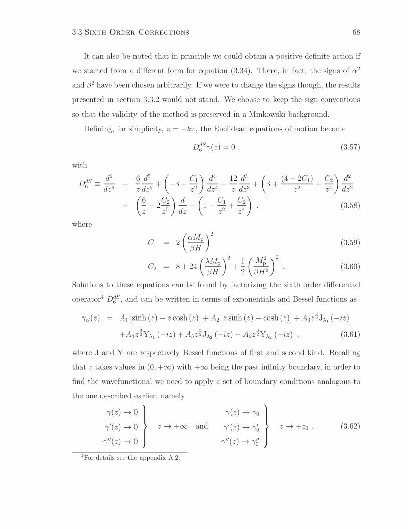
3.3 Sixth Order Corrections 68
It can also be noted that in principle we could obtain a positive definite action if
we started from a different form for equation (3.34). There, in fact, the signs of α2
and β2 have been chosen arbitrarily. If we were to change the signs though, the results
presented in section 3.3.2 would not stand. We choose to keep the sign conventions
so that the validity of the method is preserved in a Minkowski background.
Defining, for simplicity, z = −kτ , the Euclidean equations of motion become
DdS6 γ(z) = 0 , (3.57)
with
DdS6 ≡
d6
dz6+
6
z
d5
dz5+
(
−3 + C1
z2
)
d4
dz4− 12
z
d3
dz3+
(
3 +(4− 2C1)
z2+C2
z4
)
d2
dz2
+
(
6
z− 2
C2
z5
)
d
dz−(
1− C1
z2+C2
z4
)
, (3.58)
where
C1 = 2
(
αMp
βH
)2
(3.59)
C2 = 8 + 24
(
λMp
βH
)2
+1
2
(
M2p
βH2
)2
. (3.60)
Solutions to these equations can be found by factorizing the sixth order differential
operator4 DdS6 , and can be written in terms of exponentials and Bessel functions as
γcl(z) = A1 [sinh (z)− z cosh (z)] + A2 [z sinh (z)− cosh (z)] + A3z3
2Jλ1 (−iz)
+A4z3
2Yλ1 (−iz) + A5z3
2Jλ2 (−iz) + A6z3
2Yλ2 (−iz) , (3.61)
where J and Y are respectively Bessel functions of first and second kind. Recalling
that z takes values in (0,+∞) with +∞ being the past infinity boundary, in order to
find the wavefunctional we need to apply a set of boundary conditions analogous to
the one described earlier, namely
γ(z)→ 0
γ′(z)→ 0
γ′′(z)→ 0
z → +∞ and
γ(z)→ γ0
γ′(z)→ γ′0
γ′′(z)→ γ′′0
z → +z0 . (3.62)
4For details see the appendix A.2.

3.3 Sixth Order Corrections 69
The relevant classical solution of the equations of motion is therefore
γcl(z) = B1 (1 + z) e−z +B2z3
2H(2)λ1
(−iz) +B3z3
2H(2)λ2
(−iz) , (3.63)
where H(2) represents the Hankel function of the second kind, and the coefficients Bi
contain the dependence on z0 and on the boundary conditions γ0, γ′0, and γ
′′0 .
To calculate the wavefunction it is sufficient to rewrite the action as
SEdSk = [surface terms] +
∫ τ0
−∞
dτγDdS6 γ , (3.64)
so that on the classical path only the first set of terms survives, with the contribution
from the integral term being zero. Since we are ultimately interested in integrat-
ing over γ′′0 and γ′0 it is convenient to collect terms and write the wavefunctional
schematically as
ΨdS0 = N exp
[
− ik3
D(A00γ
∗0γ0 + A01γ
∗0γ
′0 + A02γ
∗0γ
′′0 + A10γ
′∗0 γ0 + A11γ
′∗0 γ
′0
+ A12γ′∗0 γ
′′0 + A20γ
′′∗0 γ0 + A21γ
′′∗0 γ
′0 + A22γ
′′∗0 γ
′′0 )
]
. (3.65)
The analytic dependence of the coefficients Aij and D on the parameters α, β, and
H/Mp appearing in the action is somewhat complicated and not very instructive, and
so we do not display this here.
To make progress analytically we now introduce an approximation scheme, taking
α, λ (if the R2 term is considered) and β to be of order unity, with H/Mp 1 playing
the role of the small parameter in a series expansion. Beside the reasonable choices
for the parameters in the action, an extra assumption is needed to simplify the calcu-
lation. We assume that β2 < 2α4, allowing us to approximate the frequencies λ1 and
λ2 and the Hankel functions. With these approximations the associated probability
takes a form similar to that of equation (3.65), with the same kinds of terms and
different coefficients. In particular, focusing on the coefficient of γ′′∗0 γ′′0 , which we
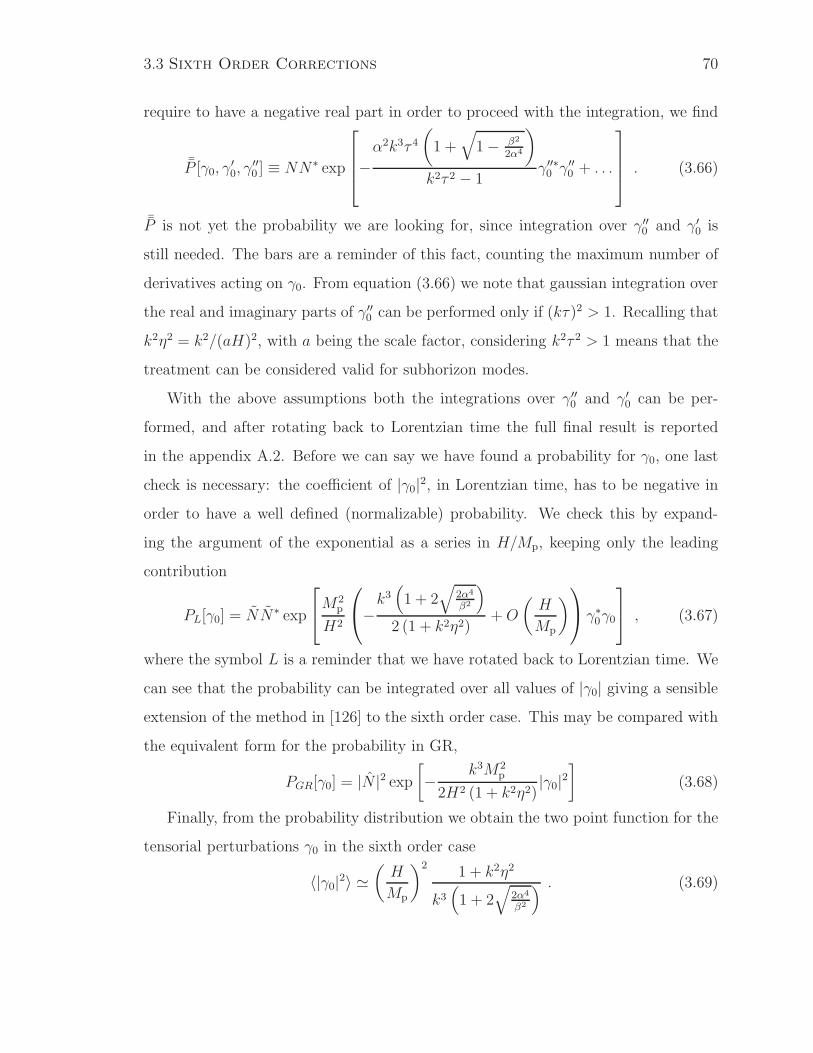
3.3 Sixth Order Corrections 70
require to have a negative real part in order to proceed with the integration, we find
¯P [γ0, γ′0, γ
′′0 ] ≡ NN∗ exp
−α2k3τ 4
(
1 +√
1− β2
2α4
)
k2τ 2 − 1γ′′∗0 γ
′′0 + . . .
. (3.66)
¯P is not yet the probability we are looking for, since integration over γ′′0 and γ′0 is
still needed. The bars are a reminder of this fact, counting the maximum number of
derivatives acting on γ0. From equation (3.66) we note that gaussian integration over
the real and imaginary parts of γ′′0 can be performed only if (kτ)2 > 1. Recalling that
k2η2 = k2/(aH)2, with a being the scale factor, considering k2τ 2 > 1 means that the
treatment can be considered valid for subhorizon modes.
With the above assumptions both the integrations over γ′′0 and γ′0 can be per-
formed, and after rotating back to Lorentzian time the full final result is reported
in the appendix A.2. Before we can say we have found a probability for γ0, one last
check is necessary: the coefficient of |γ0|2, in Lorentzian time, has to be negative in
order to have a well defined (normalizable) probability. We check this by expand-
ing the argument of the exponential as a series in H/Mp, keeping only the leading
contribution
PL[γ0] = NN∗ exp
M2p
H2
−k3(
1 + 2√
2α4
β2
)
2 (1 + k2η2)+O
(
H
Mp
)
γ∗0γ0
, (3.67)
where the symbol L is a reminder that we have rotated back to Lorentzian time. We
can see that the probability can be integrated over all values of |γ0| giving a sensible
extension of the method in [126] to the sixth order case. This may be compared with
the equivalent form for the probability in GR,
PGR[γ0] = |N |2 exp[
−k3M2
p
2H2 (1 + k2η2)|γ0|2
]
(3.68)
Finally, from the probability distribution we obtain the two point function for the
tensorial perturbations γ0 in the sixth order case
〈|γ0|2〉 '(
H
Mp
)21 + k2η2
k3(
1 + 2√
2α4
β2
) . (3.69)
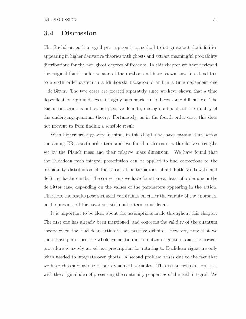
3.4 Discussion 71
3.4 Discussion
The Euclidean path integral prescription is a method to integrate out the infinities
appearing in higher derivative theories with ghosts and extract meaningful probability
distributions for the non-ghost degrees of freedom. In this chapter we have reviewed
the original fourth order version of the method and have shown how to extend this
to a sixth order system in a Minkowski background and in a time dependent one
– de Sitter. The two cases are treated separately since we have shown that a time
dependent background, even if highly symmetric, introduces some difficulties. The
Euclidean action is in fact not positive definite, raising doubts about the validity of
the underlying quantum theory. Fortunately, as in the fourth order case, this does
not prevent us from finding a sensible result.
With higher order gravity in mind, in this chapter we have examined an action
containing GR, a sixth order term and two fourth order ones, with relative strengths
set by the Planck mass and their relative mass dimension. We have found that
the Euclidean path integral prescription can be applied to find corrections to the
probability distribution of the tensorial perturbations about both Minkowski and
de Sitter backgrounds. The corrections we have found are at least of order one in the
de Sitter case, depending on the values of the parameters appearing in the action.
Therefore the results pose stringent constraints on either the validity of the approach,
or the presence of the covariant sixth order term considered.
It is important to be clear about the assumptions made throughout this chapter.
The first one has already been mentioned, and concerns the validity of the quantum
theory when the Euclidean action is not positive definite. However, note that we
could have performed the whole calculation in Lorentzian signature, and the present
procedure is merely an ad hoc prescription for rotating to Euclidean signature only
when needed to integrate over ghosts. A second problem arises due to the fact that
we have chosen γ as one of our dynamical variables. This is somewhat in contrast
with the original idea of preserving the continuity properties of the path integral. We
3.4 Discussion 72
leave to future studies the analysis of the effect of this particular choice of dynamical
variables. Third, we have considered the simplest possible scheme for taking the limit
in which the higher order terms become less important in the action; with this choice
the behaviors of the fourth and sixth order terms are locked together. A general
approximation scheme in which the two terms may go to zero independently and
introduce different corrections requires further study. Finally, note that we have only
considered one specific sixth order term in the covariant action for gravity. Although
a full calculation is needed, we do not expect the other sixth order terms to conspire
and drastically change the results found here.
Chapter 4
Anisotropic Cosmologies: Possible
Signatures in Parallax Experiments
4.1 Introduction
We have seen in the previous chapters how one may tackle some of the problems
related to cosmic acceleration during inflation and at late times, and the methods
that can be applied to slightly modify the models that describe our understanding
of the cosmological evolution. We want here to consider some completely alternative
approach to the problem of late time acceleration, and the related signatures in future
experiments. The possibly more radical main idea in this chapter is to keep GR as
is, and to relax one of the fundamental assumptions we talked about in chapter 1,
namely isotropy.
In our opinion, a particularly interesting aspect of this analysis is that the mea-
surement we discuss here belongs to a new and revolutionary class of experiments,
which could be called real time cosmology. We are in fact talking about repeated
measurements of the relative position of distant objects – quasars – with respect to
each other (cosmic “parallax”), with time baselines of the order of a decade or less.
An astonishing idea that can only exist thanks to the latest progress in experimen-
4.1 Introduction 74
tal techniques. Before we get too excited about this possibility we have to warn
the reader that our analysis suggests that upcoming experiments are not quite at
the level required to perform such measurements. We feel though that the required
precision will definitely be available in the short future, and that such “real time”
experiments will play an important role in constraining alternative proposals to the
standard model of cosmology.
As already pointed out, homogeneity and isotropy are the cornerstones of the stan-
dard cosmological model, providing not only a tremendous simplification of General
Relativity, but remarkable agreement with all observations. Homogeneity is sup-
ported by the observed galaxy distribution from large-scale structure surveys, while
isotropy is supported by, in particular, the deep spatial uniformity of the temperature
of the CMB. Nevertheless, the paradigm-changing observation of cosmic acceleration,
now more than a decade old, has forced cosmologists to re-examine even their most
cherished assumptions, including the correctness of GR as we have discussed in some
detail in previous chapters, a vanishing cosmological constant, and, more recently,
the fundamental ideas of spatial homogeneity and isotropy.
The primary evidence for the accelerating universe comes from the unexpected
dimming of type Ia supernovae [32, 132–138], as measured through their light curves.
The connection to cosmic acceleration though, requires the assumptions of homo-
geneity and isotropy, and thus this raises the possibility that abandoning one of these
principles may allow for the appearance of accelerated expansion without actual ac-
celeration itself.
Of course, the usual cosmological FLRW metric is so simple by virtue of its un-
derlying symmetries. Abandoning these leads to a correspondingly more complicated
form for the metric. It is convenient therefore to begin by studying toy models. One
class of these that has shown some promise in this direction are the Lemaıtre-Tolman-
Bondi (LTB) metrics, in which we are assumed to live inside a spherically symmetric
underdense region of spacetime (or “void”) embedded in an otherwise spatially flat
4.1 Introduction 75
and homogeneous Einstein-de Sitter universe [139–145]. Such a spacetime is mani-
festly inhomogeneous, due to the void, and on its own violates any strong version of
the Copernican principle, since we must live inside this void in order to account for
the observed supernovae dimming. Nevertheless, it has been shown that these models
can provide a satisfactory fit to the luminosity distance-redshift relation of type Ia
supernovae and the position of the first peak in the CMB [143, 146]. Thus, LTB mod-
els have been suggested as a possible solution to the problem of cosmic acceleration,
obviating the need for quintessence fields, modifications of gravity, or a cosmological
constant, and considerable effort has been devoted to constraining them [147–151].
Beyond the usual cosmological tests of homogeneity and isotropy, it has recently
been suggested that these models could be further constrained by precision mea-
surements of the evolution of the angular positions of distant sources. Following the
authors of [152], we refer to this effect as cosmic parallax. The expansion of an FLRW
universe is isotropic for all observers, and so cosmic parallax would not be observed.
Of course although our universe is very close to an FLRW universe, it is not exactly
so. For instance, on large scales bound structures may acquire small peculiar veloci-
ties, giving rise to a slight deviation from observed isotropic expansion. However, to
any observer living off-center inside the void of an LTB universe, cosmic evolution
itself is anisotropic and is an additional source of cosmic parallax. For sufficiently
off-center observers the cosmic parallax due to anisotropic expansion would dominate
over the contribution from peculiar velocities. Cosmic parallax could therefore pro-
vide an interesting test of void models. Upcoming sky surveys such as GAIA [153]
may be able to initiate a measurement of this effect, requiring only that a similar sur-
vey be completed 10 years later in order to complete the measurement. The absence
of cosmic parallax beyond what is expected from peculiar velocities would put an
upper bound on how far our galaxy could be from the center of the void in otherwise
allowed LTB models, where isotropy is restored. For example, the authors of [152]
argue that GAIA may map sufficiently many quasars, with enough accuracy, so that
4.1 Introduction 76
two such surveys spaced 10 years apart could detect the additional LTB contribution
to cosmic parallax if the Milky Way is more than 10 megaparsecs from the center of
a 1 Gpc void. If after a decade no additional contribution were found, that would
constrain the Milky Way to lie unnaturally close to the center of such a void.
On the other hand, detection of a contribution to the cosmic parallax not arising
from peculiar velocities would indicate that the expansion of the universe is aniso-
tropic from our vantage point. In LTB models this would be due to living away from
the center of the void, and the strength of the additional contribution would be re-
lated to this distance. But cosmic parallax not attributable to peculiar velocities is a
generic feature of any cosmological model with anisotropic expansion – an observation
also made in [152]. For example, spacetimes of the Bianchi type would exhibit an
additional contribution to cosmic parallax around every point. These homogeneous
and anisotropic spacetimes have recently been invoked during inflation to explain
anomalies in the CMB [154–161]1, and during late-time cosmology to describe the
expansion driven by anisotropic dark energy [163, 164]. Nevertheless, the fact that
motivations exist for studying both LTB and Bianchi spacetimes, and that both may
exhibit contributions to cosmic parallax that are not attributable to peculiar veloc-
ities, raises the question of how we might interpret any additional cosmic parallax
signal. Although an observed signal would provide evidence for deviations from an
FLRW universe, such deviations could be due to deviations from spatial homogeneity
(as in LTB models) or deviations from isotropy (as in Bianchi models). It is there-
fore of interest to consider how cosmic parallax in Bianchi models differs from LTB
models. This is what we will try to do in this chapter in the context of parallax
observations.
The structure of the chapter is as follows. In section 4.2 we briefly review the
results of [152]. In section 4.3 we describe the kinds of anisotropic models that we
will focus on; namely a subclass of Bianchi Type I models. Since we know from
1Such theories may not, however, be without problems [162].
4.2 Cosmic Parallax in an LTB Void 77
observations of the CMB that the universe is very nearly isotropic at the time of last
scattering, we describe how we restrict ourselves to Bianchi Type I metrics which
pass existing cosmological tests. In section 4.4 we derive the geodesic equations for
these spacetimes and discuss our numerical techniques for integrating them. We
then present the cosmic parallax signal we find for these models and discuss how it
compares to the cosmic parallax in void models.
4.2 Cosmic Parallax in an LTB Void
We begin by briefly reviewing how cosmic parallax manifests itself in LTB models,
as discussed in [152]. Here and throughout the rest of the chapter, unless otherwise
indicated, by cosmic parallax we mean cosmic parallax due to anisotropic expansion
about an observer. The LTB metric is given by [20–22]
ds2 = −dt2 + |R′(t, r)|2
1 + β(r)dr2 +R2(t, r)dΩ2 , (4.1)
where R(t, r) is a position-dependent scale factor, β(r) is related to the curvature
of the spatial slices, and ()′ ≡ ∂/∂r. The Einstein equations relate R(t, r) to β(r)
and an additional arbitrary function of integration α(r). Specifying α(r), β(r), and
an initial condition for R(t, r) completely determines the spacetime. In models with
an underdense region, or “void”, surrounded by an overdense region, α(r) and β(r)
roughly correspond to the width of the void and the gradient of the boundary between
the inner and outer regions, respectively, and will be specified below.
The LTB metric describes a region of spacetime that is isotropic about the origin
but inhomogeneous with respect to the radial direction. Therefore distant galaxies
appear to be receding at the same rate in all directions for observers located at the
origin. On the other hand, observers located away from the center of the void could
in principle observe anisotropic recession. One way to observe this effect [152] is to
measure how the angle between the positions of two distant sources evolves over time.
This difference is referred to as the cosmic parallax. To study this, one considers null
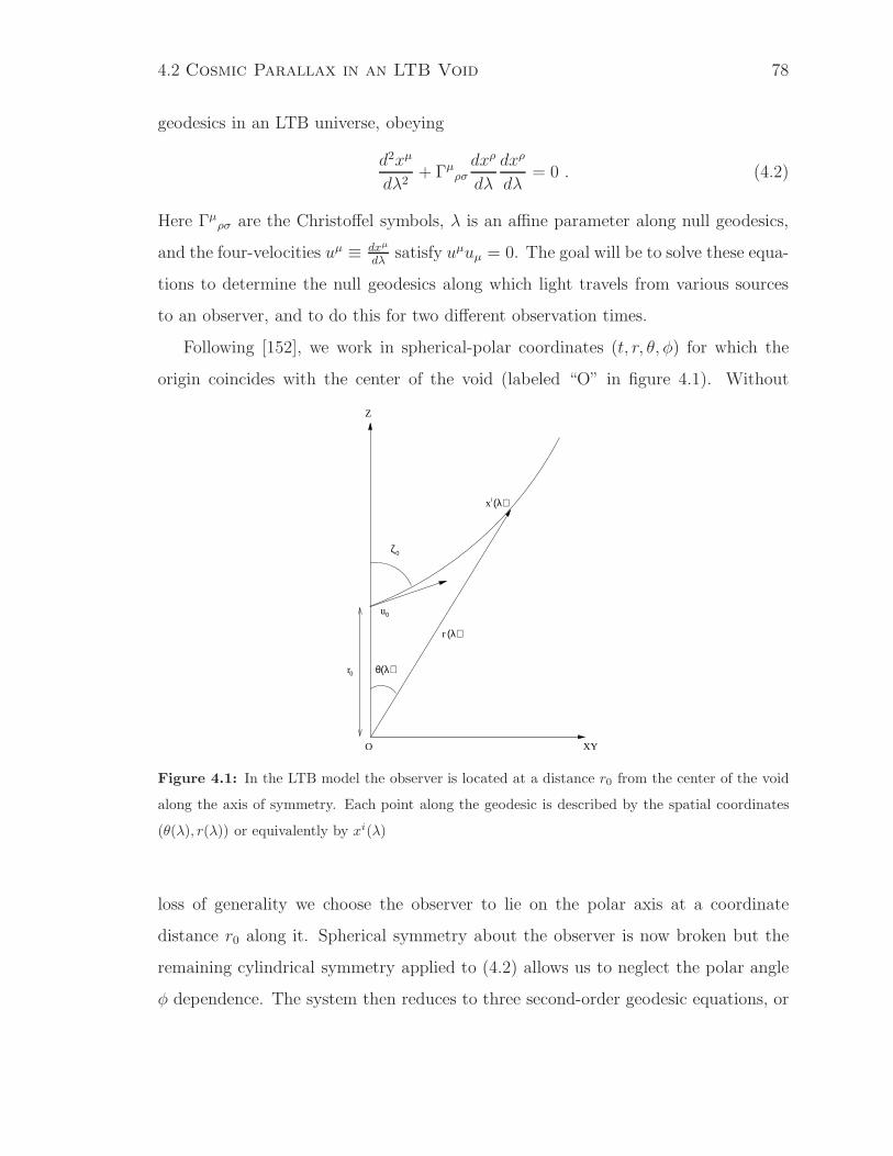
4.2 Cosmic Parallax in an LTB Void 78
geodesics in an LTB universe, obeying
d2xµ
dλ2+ Γµρσ
dxρ
dλ
dxρ
dλ= 0 . (4.2)
Here Γµρσ are the Christoffel symbols, λ is an affine parameter along null geodesics,
and the four-velocities uµ ≡ dxµ
dλsatisfy uµuµ = 0. The goal will be to solve these equa-
tions to determine the null geodesics along which light travels from various sources
to an observer, and to do this for two different observation times.
Following [152], we work in spherical-polar coordinates (t, r, θ, φ) for which the
origin coincides with the center of the void (labeled “O” in figure 4.1). Without
(λ)r
0ζ
r0
u0
(λ)xi
θ(λ)
O
Z
XY
Figure 4.1: In the LTB model the observer is located at a distance r0 from the center of the void
along the axis of symmetry. Each point along the geodesic is described by the spatial coordinates
(θ(λ), r(λ)) or equivalently by xi(λ)
loss of generality we choose the observer to lie on the polar axis at a coordinate
distance r0 along it. Spherical symmetry about the observer is now broken but the
remaining cylindrical symmetry applied to (4.2) allows us to neglect the polar angle
φ dependence. The system then reduces to three second-order geodesic equations, or
4.2 Cosmic Parallax in an LTB Void 79
equivalently six first-order equations. Applying the null geodesic condition further
reduces the system to five independent first-order equations for t, r, θ, p ≡ dr/dλ
and the redshift z as [147, 152]
dt
dλ= −
√
(R′)2
1 + βp2 +
J2
R2(4.3)
dr
dλ= p (4.4)
dθ
dλ=
J
R2(4.5)
dz
dλ=
(1 + z)√
(R′)2
1+βp2 + J2
R2
[
R′R′
1 + βp2 +
R
R3J2
]
(4.6)
dp
dλ= 2R′p
√
p2
1 + β+
(
J
RR′
)2
+1 + β
R3R′J2 +
(
β ′
2 + 2β− R′′
R′
)
p2 , (4.7)
where J ≡ R2dθ/dλ = J0, is constant along the geodesic.
To completely specify the system we require five initial conditions, which we pro-
vide for convenience at the initial observation event, and denote with a subscript “0”.
Since one would like to specify initial conditions in terms of physically measurable
quantities, we consider the angle ξ0 between the polar axis and the line of sight along
an incoming photon trajectory arriving at the observer (see figure 4.1). This angle ξ0
coincides with the coordinate angle θ when r0 = 0, but in general it is given by [147]
cos ξ0 = −R′(t, r)p
dtdλ
√
1 + β(r). (4.8)
This expression can be used to express J0 and p0 in terms of t0, r0, and ξ0, via
J0 = R(t0, r0) sin ξ0
p0 =cos ξ0
R′(t0, r0)
√
1 + β(r0) . (4.9)
Therefore, the system is completely determined by specifying t0, r0, θ0, z0, and ξ0.
Clearly, our coordinate choice means that θ0 = 0, and our conventional definition
of redshift yields z0 = 0. Following [152] we choose r0 = 15Mpc, which is the largest

4.2 Cosmic Parallax in an LTB Void 80
value consistent with the CMB dipole [147]. What remains is to specify a direction on
the sky and the time of observation to uniquely determine a geodesic that terminates
at the spacetime event of observation. This picks out an initial geodesic along which
light from a distant source travels to reach the observer.
Given the redshift and line of sight angle of a source at an initial time, we can
determine the trajectory of light from that source at a later time in the following way.
As just mentioned, the line of sight angle ξ0 picks out an initial geodesic, terminating
at the initial observation event. The observed redshift determines how far backwards
in time along this initial geodesic the source lies. We extract the comoving coordi-
nates of the source by numerically integrating backwards along this initial geodesic.
Once the comoving coordinates of the observer and source are determined, and the
interval of time between observations is specified, we solve a boundary-value problem
to determine the final geodesic. We then extract the line of sight angle of this final
geodesic ξf .
After repeating this procedure for two sources we have four angles: the input
angles ξa0 and ξb0 and the output angles ξaf and ξbf . We may then compute the
difference
∆γ ≡ γf − γ0 = (ξaf − ξbf)− (ξa0 − ξb0) , (4.10)
which is the main quantity of interest, hereafter referred to as the cosmic parallax.
In [152] this quantity is calculated for LTB models characterized by the functions
β(r) =(
HOUT0
)2r2∆α
2
(
1− tanhr − rvo2∆r
)
(4.11)
α(r) =(
HOUT0
)2r3 − rβ(r) , (4.12)
which characterize the smooth transition from the inner underdense region to the
outer, higher density region. The quantities ∆α, rvo, ∆r, and HOUT0 are free pa-
rameters of the model that can be tuned to fit CMB and supernovae measurements.
Following [152] and [143], we choose a model which is in good agreement with SNIa
observations and the location of the first peak of the CMB, namely ∆α = 0.9,
4.3 Bianchi Type I Models 81
rvo = 1.3Gpc, ∆r = 0.4 rvo, and HOUT0 = 51 km s−1Mpc−1. Although this Hub-
ble parameter outside the void seems to be in conflict with the measured Hubble
Key project value of 72 ± 8 km s−1Mpc−1 [165], one should keep in mind that the
measurements made to determine this value are all made at less than a few hundred
megaparsecs (z ≈ 0.1), whereas the size of the void in this model is about 1Gpc
(z ≈ 0.2). The Hubble parameter inside the void in this model turns out to be
65 km s−1Mpc−1, which is consistent with the Hubble Key project value. Recently
the SHOES Team [166] was able to reduce the uncertainty on the value of the Hubble
parameter to H0 = 74.2 ± 3.6 km s−1Mpc−1, raising more doubts about the validity
of this model. Although LTB models have partly motivated this study, our purpose
is not to discuss their validity. At worst, they will serve as useful toy models to study
the characteristics and magnitude of the parallax signal.
The authors of [152] numerically compute the cosmic parallax for two different
models. They find an angle-dependent signal with maximal value roughly 0.18µas
for sources at redshift of 1. It is claimed that this signal is within reach of the
forthcoming Gaia mission, provided Gaia produces a sky map of the expected number
of quasars (roughly 500, 000) with final positional error less than 30µas, and that such
measurements are repeated after 10 years.
4.3 Bianchi Type I Models
As we have discussed, anisotropic expansion of the universe around a given observer
contributes to cosmic parallax. In the case of LTB models, this may allow us to
constrain the distance of our galaxy from the center of the void. The further we
are from the center of the void, the more anisotropic the universe would look to us.
Of course, LTB spacetimes are not the only ones that can give rise to anisotropic
expansion around a point. This raises the question of how we might interpret any
observation of an anomalously large cosmic parallax, since such an observation would

4.3 Bianchi Type I Models 82
not itself be evidence that we live in an LTB universe. To understand this therefore,
we study cosmic parallax in alternative anisotropic cosmologies and compare our
results with those obtained in [152].
For simplicity we consider anisotropic spacetimes that are spatially homogeneous
[167, 168]. In particular, we focus on a subclass of Bianchi Type I spacetimes, the
metric for which may be written as
ds2 = −dt2 + a21(t)dx2 + a22(t)dy
2 + a23(t)dz2 . (4.13)
In general, a1(t), a2(t), and a3(t) are independent scale factors, describing how the
three spatial directions scale with time, which reduces to the standard FLRW case
when a1(t) = a2(t) = a3(t). We specialize to the case when only one of the scale
factors differs from the others, say a1(t) = a2(t) 6= a3(t), in which case the expansion
is axisymmetric. We do so because we want to compare our results to observations
made by an off-center observer in an LTB void. Such an observer will experience
axisymmetric cosmic expansion, and so the most direct comparison will be to an
axisymmetric Bianchi-I universe. There is, however, an important difference in the
symmetries around observers in these two spacetimes. In the axisymmetric Bianchi-I
universe there is an additional plane of symmetry normal to the axis of symmetry.
The same is not true for an off-center observer in an LTB universe. To see this, it
is sufficient to consider the extremal case of an observer outside the void, who can
obviously distinguish the two directions along the polar axis: toward the void and
away from it. This suggests that cosmic parallax in these two types of anisotropic
models will differ at least qualitatively, if not in magnitude.
Setting a1 = a2 = a(t) and a3 = b(t) in (4.13), the Einstein equations become
H2a + 2HaHb = 8πGρ (4.14)
2Ha + 3H2a = −8πGPz (4.15)
Ha + H2a + Hb +H2
b +HaHb = −8πGPx , (4.16)
where an overdot denotes a derivative with respect to t, Px = Py and Pz are anisotropic
4.3 Bianchi Type I Models 83
pressures in the different directions, and we have defined the Hubble parameters
Ha ≡ a/a and Hb ≡ b/b. The conservation of energy equation in this case is
ρ = −2Ha(ρ+ Px)−Hb(ρ+ Pz) . (4.17)
The observational success of FLRW cosmology places tight constraints on how ani-
sotropic the universe can be. In order to restrict ourselves to solutions that remain
close to an FLRW cosmology, we split each of these exact equations into an FLRW
part which evolves according the FLRW equations of motion, and a non-FLRW part
which we require to remain small, in a sense that we will now make clear. A similar
approach was used in [169]. We define
Ha(t) = H(t) + εf(t) (4.18)
Hb(t) = H(t) + εg(t) (4.19)
ρ(t) = ρ(t) + εr(t) (4.20)
Px(t) = Py(t) = P (t) (4.21)
Pz(t) = P (t) + εs(t) (4.22)
where overbars denote the FLRW quantities and ε is a small perturbative param-
eter for which we will determine an upper bound later. Substituting these defini-
tions into equations (4.14)-(4.17) and collecting powers of ε gives the zeroth-order (or
background) equations, which are just the usual ones of the FLRW metric, and the
first-order equations
2H(f + 2g) = 8πGr (4.23)
6Hf + 2f = −8πGs (4.24)
3H(f + g) + f + g = 0 (4.25)
r = −3Hr − ρ(2f + g)− Hs (4.26)
These constitute four equations in four variables, but only three of these equations are
independent. To close the system we need additional information, which we obtain
4.3 Bianchi Type I Models 84
by assuming an equation of state of the form
s(t) = σr(t) (4.27)
where the parameter σ is taken to be constant. Note that this is analogous to P = wρ,
except that it relates the anisotropic component of the pressure to the non-FLRW
correction of the energy density. The value of σ will be important in determining
whether the non-FLRW parts of equations (4.23)-(4.26) grow or decay in time.
Realistic models will be those for which the amount of anisotropy is sufficiently
small in the past and present. Assuming the anisotropy is set (for example by in-
flation) to be sufficiently small at some early epoch, the question then is whether
the anisotropy grows or not. In our set-up this corresponds to asking whether the
non-FLRW parts of equations (4.23)-(4.26) grow or not, and if so, how quickly. We
will see that σ governs the general behavior of the non-FLRW quantities, but for
a given σ, the details will depend on the background (FLRW) solution. Since we
are integrating from the present up to redshifts of order 1, our background is well
described by the ΛCDM model. Using this background we can analytically find the
asymptotic behavior of the non-FLRW quantities for different values of the equation
state parameter σ.
The background energy density and pressure for ΛCDM are
ρ = ρm + ρΛ
P = −ρΛ ,
where ρm is the background energy density of matter and ρΛ is the effective energy
density of the cosmological constant. The background equations become
3H2 = 8πG(ρΛ + ρm) (4.28)
2 ˙H + 3H2 = 8πGρΛ (4.29)
˙ρm = −3Hρm . (4.30)
4.3 Bianchi Type I Models 85
The solutions can be written simply
H(t) = A coth
(
3
2At
)
(4.31)
ρm = ρΛ
[
sinh
(
3
2At
)]−2
(4.32)
A =
√
8πGρΛ3
. (4.33)
Using (4.27) and (4.23) in (4.26) then gives
r = −[
(3 + σ)A coth
(
3
2At
)
+12AπG
sinh(
32At)
]
r(t) , (4.34)
which can be integrated to find
r(t) = c1 cosh
(
3
2At
)[
sinh
(
3
2At
)]−(3+ 2
3σ)
. (4.35)
Using the equation of state (4.27) immediately gives s(t). Equations (4.24) and (4.25)
can then be integrated to find the remaining solutions (for σ 6= −9/2)
f(t) =A
[
sinh(
32At)]2
c2 +3c1
2[
sinh(
32At)] 2
3σ
(4.36)
g(t) = −f(t)− Ac2[
sinh(
32At)]2 . (4.37)
Now we consider the asymptotic behavior of these solutions for t→∞ and t→ 0 in
turn.
The behavior as t→∞ is
r(t) ∼ s(t) ∼ c1
[
sinh
(
3
2At
)]−2(1+ 1
3σ)
. (4.38)
f(t) ∼ −g(t) ∼ c1
[
sinh
(
3
2At
)]Max[−2,−2(1+ 1
3σ)]
. (4.39)
Here we see that σ = −3 is the boundary between growing and decaying solutions. If
we require all of the non-FLRW quantities to decay as t→∞, then we must restrict
ourselves to σ > −3.
4.3 Bianchi Type I Models 86
As t → 0, the situation is slightly more complicated. The behavior of f(t) and
g(t) have a part that depends on the value of σ and a part that does not. The part
that does not behaves as
c2A
[
sinh(
32At)]2 ∼ c2t
−2 , t→ 0 ,
whereas the part that depends on σ behaves as
c13A
2[
sinh(
32At)]2(1+ 1
3σ)∼ c1t
−2(1+ 1
3σ) , t→ 0 .
We require that the expansion history is close to FLRW in the far past, which amounts
to demanding that |f/H|, |g/H|, etc remain . O(1) as t → 0. From the first term,
this requires that c2 = 0, while the second term requires that σ < −3/2. Therefore
solutions with decaying anisotropy have an equation of state parameter lying in the
range −3 < σ < −3/2. Turning to r(t) and s(t), as t→ 0 we have
r(t) ∼ s(t) ∼ c1
[
sinh
(
3
2At
)]−(3+ 2
3σ)
. (4.40)
When σ > −3 these solutions diverge as t→ 0, but if σ < −3/2 they diverge slower
than ρ and P , respectively. So the condition
−3 < σ < −32
(4.41)
will ensure that all non-FLRW quantities remain small in the far past, as required.
We will restrict ourselves to these models in the rest of this chapter.
What remains is to fix c1 and the constant A in the solutions (4.35)-(4.37). We do
this by imposing observational constraints on the models of interest. First we impose
a condition at the surface of last scattering. For an anisotropically expanding universe
to be viable it must at the very least predict angular variations in the temperature of
the CMB no bigger than 10−5. We can estimate the maximum temperature difference
at the time of last scattering by
∆T0 = |T xy0 − T z0 |
=
∣
∣
∣
∣
Tlss
(
alssa0
)
− Tlss(
blssb0
)∣
∣
∣
∣
, (4.42)
4.3 Bianchi Type I Models 87
where T z is the temperature along the axis of symmetry and T xy is the temperature
in the transverse plane; subscripts “0” and “lss” refer to quantities today and at the
last scattering surface, respectively. Recall that b(t) is the scale factor along the axis
of symmetry and a(t) is the scale factor in the transverse plane. From the definitions
of Ha and Hb, we have
a(t) = a0 exp
∫ t
t0
(H(t′) + εf(t′))dt′ (4.43)
b(t) = b0 exp
∫ t
t0
(H(t′) + εg(t′))dt′ . (4.44)
Using these, and choosing a0 = b0 = 1, we can re-write the expression for ∆T0 to first
order in ε as
∆T0 = Tlss
(
blssb0
) ∣
∣
∣
∣
1−(
alssblss
b0a0
)∣
∣
∣
∣
' 2εT z0
∣
∣
∣
∣
∫ tlss
t0
f(t)dt
∣
∣
∣
∣
, (4.45)
where we have used the fact that g(t) = −f(t), which is a consequence of requiring
c2 = 0. Inserting the solution for f(t) gives
∆T0T z0' 3Aεc1
∫ tlss
t0
[
sinh
(
3
2At
)]−2(1+σ3)
dt . (4.46)
Demanding the left-hand side to be at most 1.3× 10⁻⁶ [170] yields one condition on
the product εc1 and A for a given equation of state parameter σ.
In order to break the degeneracy between εc1 and A, we need one further condition.
Equation (4.46) already requires the difference between Ha and Hb to be small – well
within the accepted uncertainty in the measured value of the Hubble parameter [166].
We find it convenient to choose to set the arithmetic average of the Hubble parameters
in the three directions equal to the observed value.
Hobs =2Ha +Hb
3
= H +ε
3f(t) , (4.47)
where again we have used the fact that when c2 = 0, g(t) = −f(t). Alternative
choices, such as settingHa orHb equal to the measured value of the Hubble parameter,
4.3 Bianchi Type I Models 88
would not change the order of magnitude of εc1 and A and would leave the final result
essentially unaltered. Inserting the solution for f(t) into equation (4.47) gives a second
condition on εc1 and A
εc1 =2
A(Hobs − H)
[
sinh
(
3
2At
)]2(1+σ3)
. (4.48)
We can (numerically) solve this equation for A in terms of εc1 and then substitute it
back into the first condition (4.46) to obtain an upper bound on εc1. By taking the
maximal allowed value for εc1, we can then find A using (4.48). For σ = −2 we find
A ' 62(km/s)/Mpc and εc1 ' 1.3 × 10⁻⁶. We always take c1 to be O(1), and so in
this case we choose c1 = 1.3 and ε = 10−6.
In this way we can fully determine solutions to the non-FLRW quantities for a
given equation of state parameter σ. By restricting ourselves to −3 < σ < −3/2 we
have chosen to focus on models for which these solutions decay in the distant future
and which diverge slower than the respective background quantities in the far past as
one approaches the initial singularity. These models seem to be the most conservative
realizations of a Bianchi-I cosmology, in the sense that they are the easiest to make
consistent with observations, or alternatively, the most difficult to rule out. One
might try to push the boundaries slightly, for example by considering models with
anisotropies that approach a constant in the distant future rather than vanishing.
It may be that such models can be carefully tuned to match observations. We do
not consider these more general models here, since our main interest is not model-
building, but rather to explore a general effect (cosmic parallax) arising in a Bianchi-I
universe.
4.4 Geodesics and Parallax in Axisymmetric Bianchi-I Models 89
4.4 Geodesics and Parallax in Axisymmetric
Bianchi-I Models
As in section 4.2, in order to analyze cosmic parallax we need to find null geodesics
in the spacetime that connect an observer and various sources at two different times.
As before, letting latin indices run over 1, 2, 3 and (x0, x1, x2, x3) = (t, x, y, z), the
non-zero Christoffel symbol components for the Bianchi-I metric in (4.13) are
Γ0ij = a2iHiδij , Γi0j = Hiδ
ij ,
where no sum on the index i is implied and Hi is defined as above. The four geodesic
equations are then
d2t
dλ2= −
∑
i
Hi
(
aidxi
dλ
)2
(4.49)
d2xi
dλ2= −2Hi
dt
dλ
dxi
dλ, (4.50)
with the null geodesic condition, uµuµ = 0, becoming
(
dt
dλ
)2
=∑
i
(
aidxi
dλ
)2
. (4.51)
As before, uµ ≡ dxµ/dλ. We specialize to the axisymmetric case by setting a1 = a2 =
a(t) and a3 = b(t), and also H1 = H2 = Ha and H3 = Hb. The scale factors, a(t) and
b(t), and Hubble parameters, Ha(t) and Hb(t), are fixed after choosing σ and solving
the full set of equations as in the previous section.
After fixing the background Bianchi-I spacetime, equations (4.49) and (4.50) yield
four second-order differential equations and one constraint equation in four dependent
variables. To solve this system we must in principle specify initial conditions for the
four dependent variables as well as initial velocities (derivatives with respect to λ)
giving a total of eight conditions. However, using the constraint equation the system
can be reduced to seven independent first-order equations.
4.4 Geodesics and Parallax in Axisymmetric Bianchi-I Models 90
Considering the uµ(t) ≡ dxµ(t)/dλ as functions of time along the geodesic, equa-
tions (4.50) can be integrated immediately to give
ui(t) = ui0 e−2
∫ t
t0Hi(t′)dt′
= ui0 a−2i (t) , (4.52)
which can then be used in equation (4.51) to give
(
dt
dλ
)2
=∑
i
(
ui0ai(t(λ))
)2
. (4.53)
As in the LTB case it is again useful to find an expression for the redshift as it will
be one of our observational inputs. To find this expression, as usual, we consider
two photons emitted from a source at times t and t + τ , respectively, where τ is
taken to be infinitesimally small. The trajectory of the first photon is described
by equation (4.53), while to first order in τ , the trajectory of the second photon is
described by the geodesic equation(
dt
dλ
)2
+ 2dt
dλ
dτ
dλ=∑
i
(
uiai)2
(1 + 2τHi) . (4.54)
Here the variation in time corresponds to a time-delay, and so to a change in geodesic,
and not to a change of the time coordinate along a fixed geodesic. Since the ui(λ)
are directional derivatives along a given geodesic, they remain unaffected by time
variations (derivatives) in obtainig this equation. Using the standard definition of
redshift, 1 + z(λem) ≡ τ(λob)/τ(λem), we find the relation
d log(1 + z(λem))
dλem= − 1
τ(λem)
dτ(λem)
dλem, (4.55)
where λem and λob are the values of the affine parameter at the emission and obser-
vation event, respectively. Using this in (4.54) gives
d log(1 + z)
dλ= −
∑
i (uiai)
2Hi
√
∑
i (uiai)
2
=d log
√
∑
i (uiai)
2
dλ. (4.56)

4.4 Geodesics and Parallax in Axisymmetric Bianchi-I Models 91
In the last step we have also made use of (4.52) and the chain rule
d
dλ(ui(λ)ai(λ)) = − dt
dλ(ui(t)ai(t)Hi(t)) .
With the initial condition z(λ0) = 0, integrating (4.56) then gives
(1 + z) =
√
∑
i (uiai)
2
√
∑
i (ui0)
2. (4.57)
As in section 4.2, we would like to express our results not only in terms of redshift
but also in terms of angles, since these are the actual observables. In general there
are four pieces of data for each object in the sky, namely the time of observation, two
angles with respect to an arbitrary coordinate system, and the observed redshift of
the source. In the case of cylindrical symmetry one angle is enough. In contrast with
LTB spacetimes, not much is gained in this case by rewriting the geodesic equations
in terms of angles and redshift. Instead, we numerically integrate the equations in
the above coordinates and then express the results in terms of angles and redshift.
Our procedure for computing the cosmic parallax for these models is analogous
to that in section 4.2. We work in local Cartesian coordinates (t, x1, x2, x3) in which
the observer is located at the origin. As seen above, the system of four second-
order differential equations plus a constraint reduces to seven independent first-order
equations, some of which can be integrated immediately by hand. We are then left
with the problem of fixing initial conditions for our complete set of equations
dt
dλ= −
√
∑
i
(uiai)2 (4.58)
ui(λ) =ui0a2i
(4.59)
dxi
dλ= ui , (4.60)
where the subscripts “0” refer to quantities at the initial observation event, corre-
sponding to λ = 0. To close the system requires seven initial conditions that unfor-
tunately cannot be all specified at the observation event. By construction we have
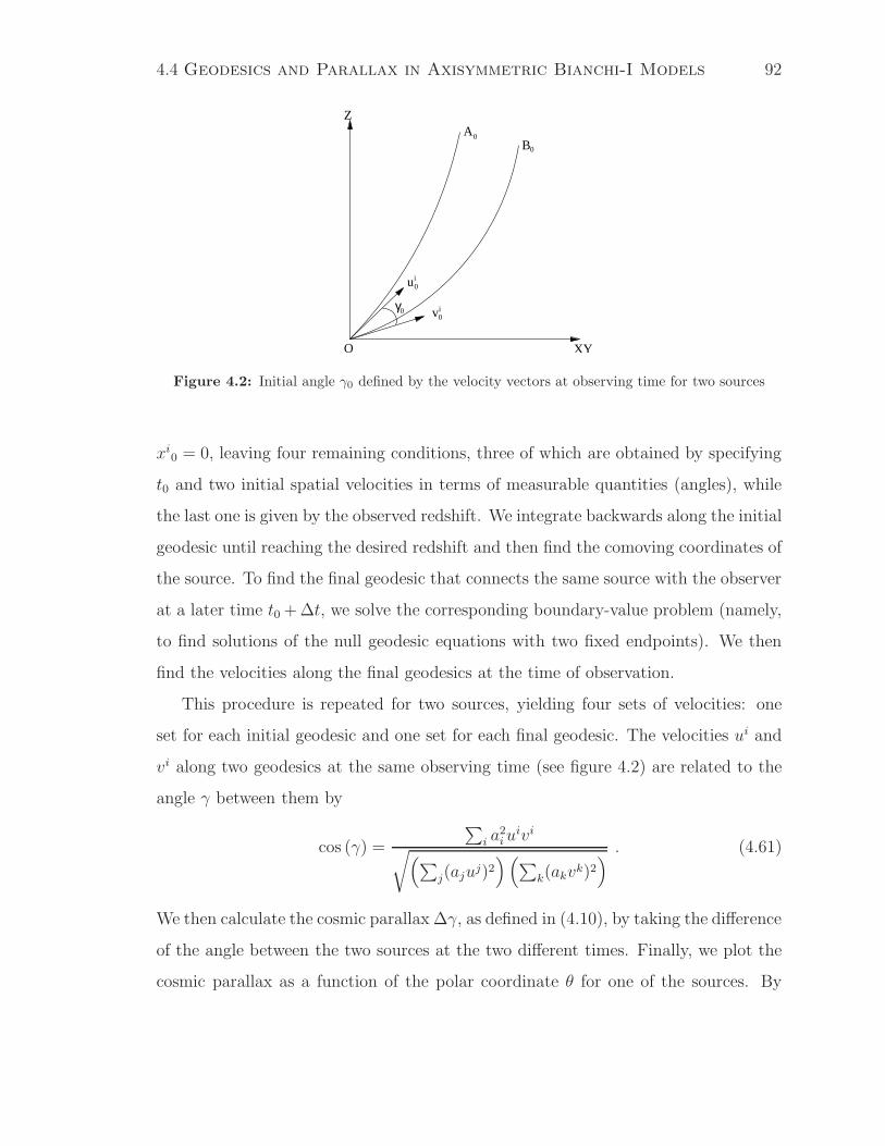
4.4 Geodesics and Parallax in Axisymmetric Bianchi-I Models 92
vi0
u0i
γ0
A0B0
XYO
Z
Figure 4.2: Initial angle γ0 defined by the velocity vectors at observing time for two sources
xi0 = 0, leaving four remaining conditions, three of which are obtained by specifying
t0 and two initial spatial velocities in terms of measurable quantities (angles), while
the last one is given by the observed redshift. We integrate backwards along the initial
geodesic until reaching the desired redshift and then find the comoving coordinates of
the source. To find the final geodesic that connects the same source with the observer
at a later time t0 +∆t, we solve the corresponding boundary-value problem (namely,
to find solutions of the null geodesic equations with two fixed endpoints). We then
find the velocities along the final geodesics at the time of observation.
This procedure is repeated for two sources, yielding four sets of velocities: one
set for each initial geodesic and one set for each final geodesic. The velocities ui and
vi along two geodesics at the same observing time (see figure 4.2) are related to the
angle γ between them by
cos (γ) =
∑
i a2iu
ivi√
(
∑
j(ajuj)2)(
∑
k(akvk)2)
. (4.61)
We then calculate the cosmic parallax ∆γ, as defined in (4.10), by taking the difference
of the angle between the two sources at the two different times. Finally, we plot the
cosmic parallax as a function of the polar coordinate θ for one of the sources. By
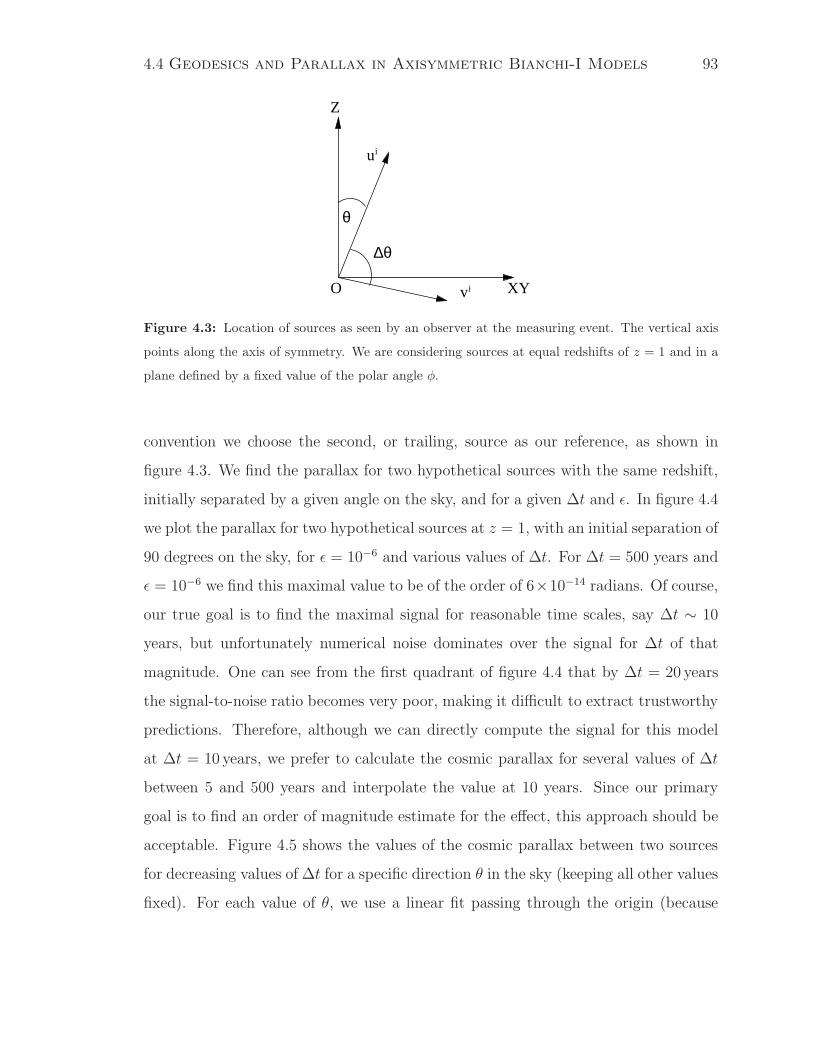
4.4 Geodesics and Parallax in Axisymmetric Bianchi-I Models 93
ui
vi
θ
∆θ
O XY
Z
Figure 4.3: Location of sources as seen by an observer at the measuring event. The vertical axis
points along the axis of symmetry. We are considering sources at equal redshifts of z = 1 and in a
plane defined by a fixed value of the polar angle φ.
convention we choose the second, or trailing, source as our reference, as shown in
figure 4.3. We find the parallax for two hypothetical sources with the same redshift,
initially separated by a given angle on the sky, and for a given ∆t and ε. In figure 4.4
we plot the parallax for two hypothetical sources at z = 1, with an initial separation of
90 degrees on the sky, for ε = 10−6 and various values of ∆t. For ∆t = 500 years and
ε = 10−6 we find this maximal value to be of the order of 6×10⁻¹⁴ radians. Of course,
our true goal is to find the maximal signal for reasonable time scales, say ∆t ∼ 10
years, but unfortunately numerical noise dominates over the signal for ∆t of that
magnitude. One can see from the first quadrant of figure 4.4 that by ∆t = 20 years
the signal-to-noise ratio becomes very poor, making it difficult to extract trustworthy
predictions. Therefore, although we can directly compute the signal for this model
at ∆t = 10 years, we prefer to calculate the cosmic parallax for several values of ∆t
between 5 and 500 years and interpolate the value at 10 years. Since our primary
goal is to find an order of magnitude estimate for the effect, this approach should be
acceptable. Figure 4.5 shows the values of the cosmic parallax between two sources
for decreasing values of ∆t for a specific direction θ in the sky (keeping all other values
fixed). For each value of θ, we use a linear fit passing through the origin (because
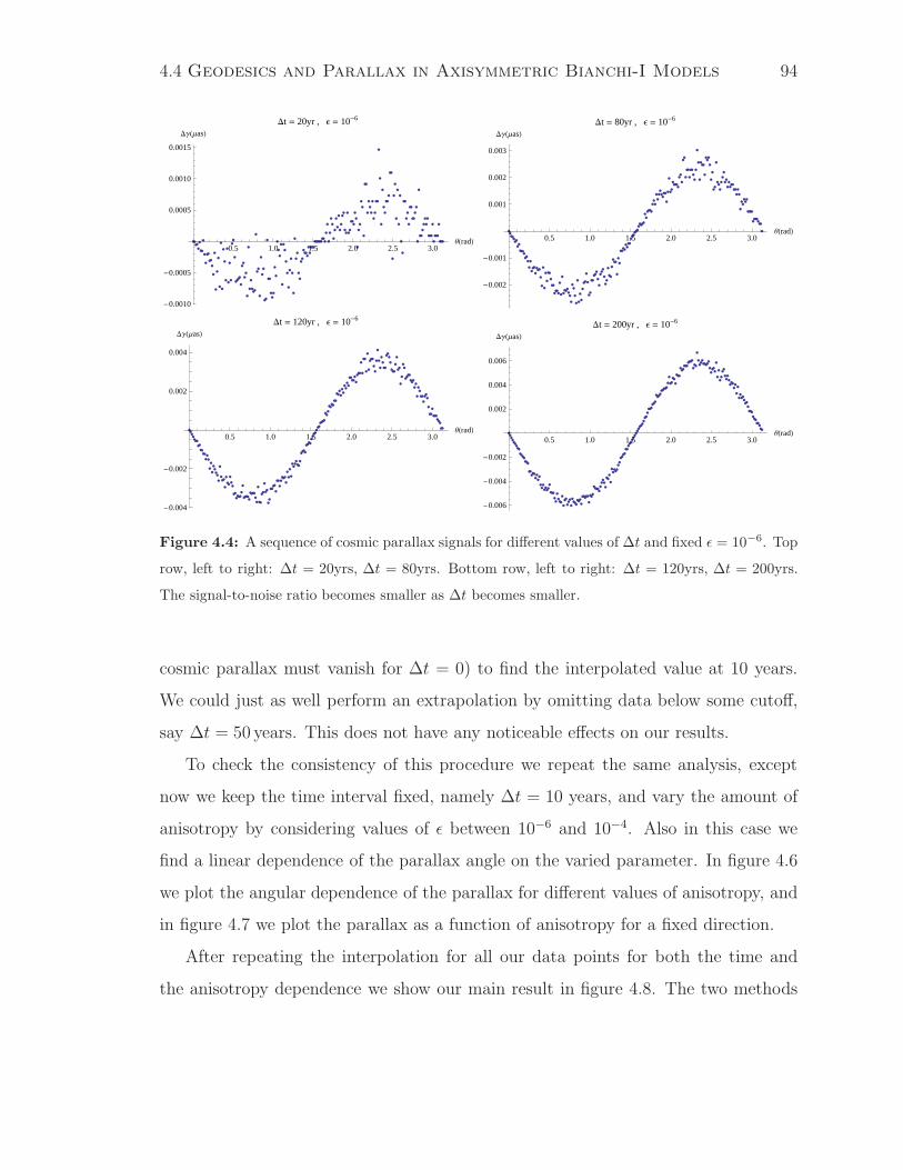
4.4 Geodesics and Parallax in Axisymmetric Bianchi-I Models 94
0.5 1.0 1.5 2.0 2.5 3.0ΘHradL
-0.0010
-0.0005
0.0005
0.0010
0.0015
DΓHΜasL
Dt = 20yr , Ε = 10-6
0.5 1.0 1.5 2.0 2.5 3.0ΘHradL
-0.002
-0.001
0.001
0.002
0.003
DΓHΜasL
Dt = 80yr , Ε = 10-6
0.5 1.0 1.5 2.0 2.5 3.0ΘHradL
-0.004
-0.002
0.002
0.004
DΓHΜasL
Dt = 120yr , Ε = 10-6
0.5 1.0 1.5 2.0 2.5 3.0ΘHradL
-0.006
-0.004
-0.002
0.002
0.004
0.006
DΓHΜasL
Dt = 200yr , Ε = 10-6
Figure 4.4: A sequence of cosmic parallax signals for different values of ∆t and fixed ε = 10−6. Top
row, left to right: ∆t = 20yrs, ∆t = 80yrs. Bottom row, left to right: ∆t = 120yrs, ∆t = 200yrs.
The signal-to-noise ratio becomes smaller as ∆t becomes smaller.
cosmic parallax must vanish for ∆t = 0) to find the interpolated value at 10 years.
We could just as well perform an extrapolation by omitting data below some cutoff,
say ∆t = 50 years. This does not have any noticeable effects on our results.
To check the consistency of this procedure we repeat the same analysis, except
now we keep the time interval fixed, namely ∆t = 10 years, and vary the amount of
anisotropy by considering values of ε between 10−6 and 10−4. Also in this case we
find a linear dependence of the parallax angle on the varied parameter. In figure 4.6
we plot the angular dependence of the parallax for different values of anisotropy, and
in figure 4.7 we plot the parallax as a function of anisotropy for a fixed direction.
After repeating the interpolation for all our data points for both the time and
the anisotropy dependence we show our main result in figure 4.8. The two methods
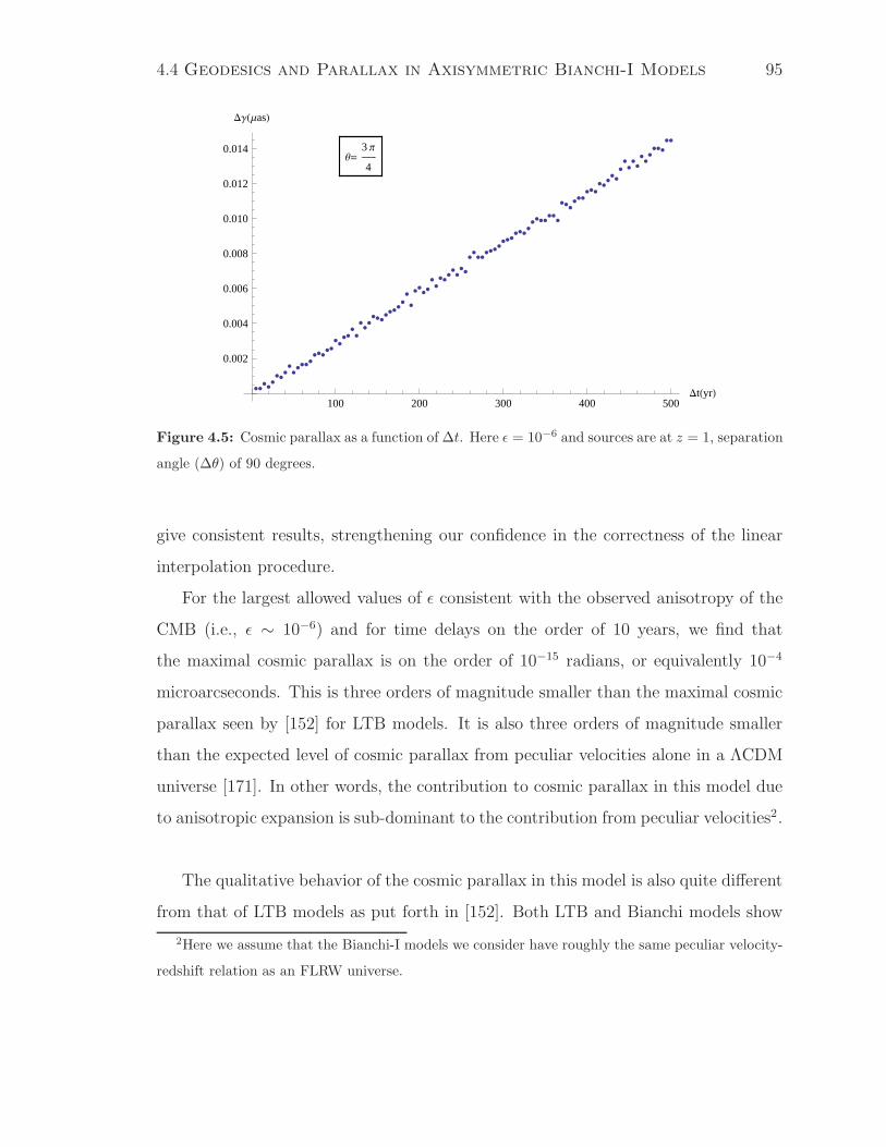
4.4 Geodesics and Parallax in Axisymmetric Bianchi-I Models 95
Θ= 3 Π
4
100 200 300 400 500DtHyrL
0.002
0.004
0.006
0.008
0.010
0.012
0.014
DΓHΜasL
Figure 4.5: Cosmic parallax as a function of ∆t. Here ε = 10−6 and sources are at z = 1, separation
angle (∆θ) of 90 degrees.
give consistent results, strengthening our confidence in the correctness of the linear
interpolation procedure.
For the largest allowed values of ε consistent with the observed anisotropy of the
CMB (i.e., ε ∼ 10−6) and for time delays on the order of 10 years, we find that
the maximal cosmic parallax is on the order of 10−15 radians, or equivalently 10−4
microarcseconds. This is three orders of magnitude smaller than the maximal cosmic
parallax seen by [152] for LTB models. It is also three orders of magnitude smaller
than the expected level of cosmic parallax from peculiar velocities alone in a ΛCDM
universe [171]. In other words, the contribution to cosmic parallax in this model due
to anisotropic expansion is sub-dominant to the contribution from peculiar velocities2.
The qualitative behavior of the cosmic parallax in this model is also quite different
from that of LTB models as put forth in [152]. Both LTB and Bianchi models show
2Here we assume that the Bianchi-I models we consider have roughly the same peculiar velocity-
redshift relation as an FLRW universe.
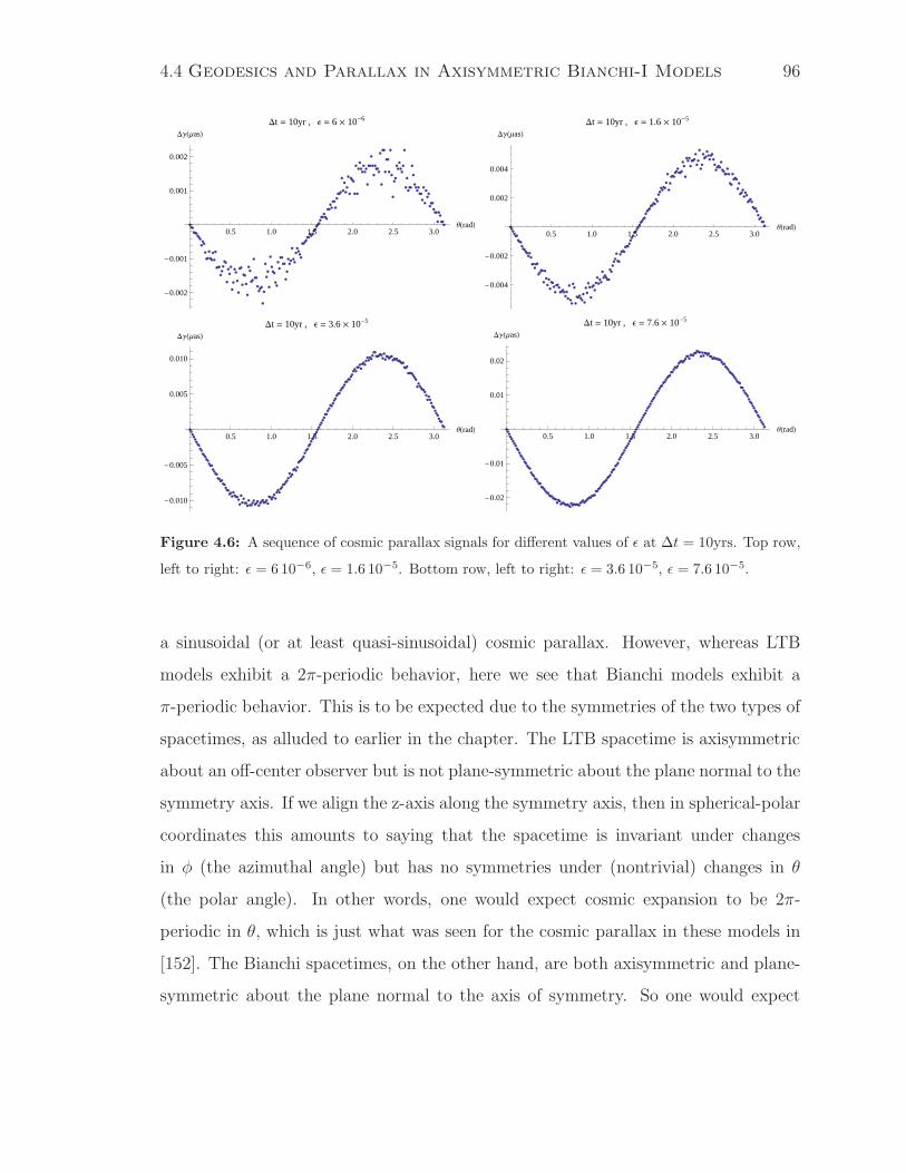
4.4 Geodesics and Parallax in Axisymmetric Bianchi-I Models 96
0.5 1.0 1.5 2.0 2.5 3.0ΘHradL
-0.002
-0.001
0.001
0.002
DΓHΜasL
Dt = 10yr , Ε = 6 ´ 10-6
0.5 1.0 1.5 2.0 2.5 3.0ΘHradL
-0.004
-0.002
0.002
0.004
DΓHΜasL
Dt = 10yr , Ε = 1.6 ´ 10-5
0.5 1.0 1.5 2.0 2.5 3.0ΘHradL
-0.010
-0.005
0.005
0.010
DΓHΜasL
Dt = 10yr , Ε = 3.6 ´ 10-5
0.5 1.0 1.5 2.0 2.5 3.0ΘHradL
-0.02
-0.01
0.01
0.02
DΓHΜasL
Dt = 10yr , Ε = 7.6 ´ 10-5
Figure 4.6: A sequence of cosmic parallax signals for different values of ε at ∆t = 10yrs. Top row,
left to right: ε = 6 10−6, ε = 1.6 10−5. Bottom row, left to right: ε = 3.6 10−5, ε = 7.6 10−5.
a sinusoidal (or at least quasi-sinusoidal) cosmic parallax. However, whereas LTB
models exhibit a 2π-periodic behavior, here we see that Bianchi models exhibit a
π-periodic behavior. This is to be expected due to the symmetries of the two types of
spacetimes, as alluded to earlier in the chapter. The LTB spacetime is axisymmetric
about an off-center observer but is not plane-symmetric about the plane normal to the
symmetry axis. If we align the z-axis along the symmetry axis, then in spherical-polar
coordinates this amounts to saying that the spacetime is invariant under changes
in φ (the azimuthal angle) but has no symmetries under (nontrivial) changes in θ
(the polar angle). In other words, one would expect cosmic expansion to be 2π-
periodic in θ, which is just what was seen for the cosmic parallax in these models in
[152]. The Bianchi spacetimes, on the other hand, are both axisymmetric and plane-
symmetric about the plane normal to the axis of symmetry. So one would expect

4.4 Geodesics and Parallax in Axisymmetric Bianchi-I Models 97
Θ= 3 Π
4
0.00002 0.00004 0.00006 0.00008Ε
0.005
0.010
0.015
0.020
0.025
DΓHΜasL
Figure 4.7: Cosmic parallax as a function of ε for a fixed value of ∆t = 10yrs.
cosmic expansion to be π-periodic in θ, which is what we see for the cosmic parallax
in these models.
Although here we have only considered a particular model, preliminary investiga-
tions into other models suggest that these results are robust. For example, one might
consider models with other constant values for the equation of state parameter σ, a
time-varying rather than constant σ, or an equation of state that takes a different
form than equation (4.27). None of these modifications seem to affect the order of
magnitude of the cosmic parallax (which, due to the symmetry of the metric, is the
only free parameter). What this suggests is that the contribution to the cosmic par-
allax from viable Bianchi-I models is much smaller than the contribution from viable
LTB-void models. If the observed cosmic parallax deviates from what is expected in
an FLRW universe, it is unlikely that this is due to our living in a Bianchi-I spacetime.
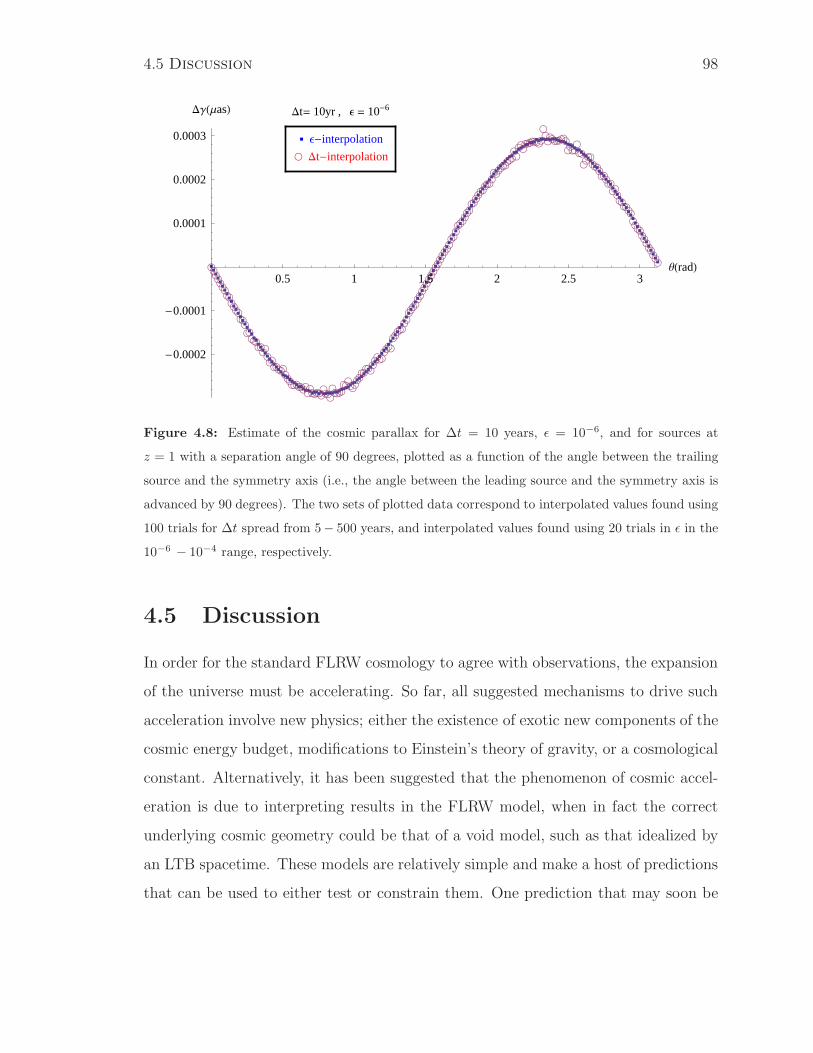
4.5 Discussion 98
ääääääääääääääääääääääääääääääääääääääääääääääääääääääääää
ääääääääääääääääääääääääääääääääääääääääääääääääääääääääääääääääääääääääääääääääääääääääääääääääääääääääääääääääääääääääääääää
ääääääääääääääää
ççççççççççççççççççççççççççççççççççççççççççççççççççççççççççççççççççççççççççççççççç
ççççççççççççççççççççççççççççççççççççççççççççççççççççççççççççççççççç
çççççççççççççççççç
çççççççççççççççççççççççççççççççççç
0.5 1 1.5 2 2.5 3ΘHradL
-0.0002
-0.0001
0.0001
0.0002
0.0003
DΓHΜasL Dt= 10yr , Ε = 10-6
ä Ε-interpolation
ç Dt-interpolation
Figure 4.8: Estimate of the cosmic parallax for ∆t = 10 years, ε = 10−6, and for sources at
z = 1 with a separation angle of 90 degrees, plotted as a function of the angle between the trailing
source and the symmetry axis (i.e., the angle between the leading source and the symmetry axis is
advanced by 90 degrees). The two sets of plotted data correspond to interpolated values found using
100 trials for ∆t spread from 5− 500 years, and interpolated values found using 20 trials in ε in the
10−6 − 10−4 range, respectively.
4.5 Discussion
In order for the standard FLRW cosmology to agree with observations, the expansion
of the universe must be accelerating. So far, all suggested mechanisms to drive such
acceleration involve new physics; either the existence of exotic new components of the
cosmic energy budget, modifications to Einstein’s theory of gravity, or a cosmological
constant. Alternatively, it has been suggested that the phenomenon of cosmic accel-
eration is due to interpreting results in the FLRW model, when in fact the correct
underlying cosmic geometry could be that of a void model, such as that idealized by
an LTB spacetime. These models are relatively simple and make a host of predictions
that can be used to either test or constrain them. One prediction that may soon be
4.5 Discussion 99
testable is cosmic parallax. For observers located 10 Mpc from the center of a 1 Gpc
LTB void, this effect would have a magnitude of the order of 10−1µas per decade for
sources at redshift 1. Since the effect in an FLRW universe (due to peculiar velocities)
is expected to be roughly the same order of magnitude, one might hope to subtract
the signal due to peculiar velocities from the signal due to anisotropic expansion
about a point. Measuring this additional contribution to the cosmic parallax would
clearly indicate a departure from FLRW.
However, what is less clear is how we might interpret detection of an additional
contribution to cosmic parallax. Here we have examined an axisymmetric Bianchi-I
universe as an alternative explanation for any cosmic parallax component that is not
attributable to peculiar velocities. We find that for a class of models whose anisotropy
is consistent with the observed temperature anisotropies of the CMB and Hubble ex-
pansion today, the maximum amount of cosmic parallax is three orders of magnitude
smaller than the maximal signal in LTB models. Perhaps more importantly, the
maximum effect is also three orders of magnitude smaller than the expected level of
cosmic parallax from peculiar velocities in an FLRW universe. Although we have
focused our discussion in this chapter on a particular model, we have found these
results to be fairly model-independent. Thus it seems unlikely that measurements
of cosmic parallax can constrain Bianchi-I models that are not already ruled out
by the CMB or other cosmological observations. Therefore, while cosmic parallax
will be nonzero for any anisotropic expansion, the magnitude of the effect suggested
in [152] appears to be significantly larger, and qualitatively different than in the class
of models considered here.
Conclusions
General Relativity and Field Theory are the basics tools cosmologists can use to de-
scribe the universe. In this framework, fields describing matter as well as corrections
to the background geometry are treated as quantum objects living in an otherwise un-
perturbed classical background fully described by some classical GR solution. Luckily
enough, this treatment seems to be sufficient to take into account the main features
of cosmological systems, as encoded in the standard model of cosmology.
During most of the evolution of the universe, GR does an incredibly good job in
providing the right background for all the physical phenomena that cosmologists and
astro-physicists are interested in. It only fails where by definition it is expected to
fail, namely when a full quantum theory of gravity is required as the times under
exam are too close to the initial singularity. The need for a more fundamental theory
though, is not the only reason why physicists venture into the research of alternative
descriptions and models. The more data, the more special features of our universe
emerge, and suggest that the simplest description may not be suitable to provide an
explanation of what we see in the sky.
In order to go beyond the simplest description, there are only few possible steps
that can be taken. One way to proceed is to consider modifications of the theory of
gravity, and propose alternative descriptions such as scalar-tensor theories, bouncing
cosmologies, or even inhomogeneous models. Each of these ideas has been proposed
to address some specific problem or feature such as late time acceleration, inflation
with a proper end and reheating of the universe, and so on. Another way to proceed
4.5 Discussion 101
which we have discussed here is via the parametrization of the unknown by using
the effective field theory approach. The great advantage of this bottom-up point of
view is the wide scope of application, as it can be used for calculating predictions
for all of the above mentioned problems, as well as any other physical features for
which nonlinearities are not strong and a series expansion makes sense – a necessary
assumption to obtain sensible results for corrections of the “zeroth-order theory”.
Chapter 2 of this work describes the application of the effective field theory ap-
proach to the study of the validity of perturbation theory during the inflationary early
stages of the universe. The aim was finding when perturbations cease to be such and
the formalism breaks down. In other words we have looked for an estimate of the
upper momentum cutoff for the inflating theory when the background considered is
not fully Lorentz-invariant. We have found that the perturbative expansion holds to
higher physical momenta than naıvely expected.
In chapter 3, we adopted a more radical point of view in modifying gravity, and
allowed for the existence of extra degrees of freedom. Via an intricate regularization
scheme we have calculated the corrections to the GR description of late time accel-
eration due to the extra degrees of freedom. In particular we have considered the
effect of a sixth order term to check the consistency of the Euclidean path integral
method at orders higher than four. We have found that in an accelerated background
ambiguities emerge and that, if this method is applied to all orders, perturbations
grow at higher orders leading to a divergent result.
Finally in chapter 4, we considered an alternative approach to the interpretation
of supernovae dimming. We have studied an anisotropic universe described by a
Bianchi-I model and its signature on a parallax proposed experiment. We have then
compared the results of our calculations and simulations with similar studies for LTB
models that share some similarities with the one considered, and showed that the
signatures of these models are in principle different in shape. We have also discussed
the magnitude of cosmic parallax for viable anisotropic models, and showed it to be
4.5 Discussion 102
orders of magnitude smaller than in the case of LTB.
While in the work we have restricted our attention to particular problems and
areas of cosmology, such as early and late time acceleration, we point out that the
analyzed methods apply in general to almost any topic in cosmology. As we tried
to stress in chapter 1 introduction, the EFT approach can be applied to any system
either to integrate out some degrees of freedom that do not participate in the process
under consideration (see for example heavy fields that at low energies effectively
work as possibly classical spectators for the physics of other lighter ones), or to
parametrize what is assumed to exist in the spectrum of a more fundamental theory
at higher energies. Higher dimensional theories are a typical example. In these
models extra dimensions beside the four that we experience in everyday life have
some effect on the physics that we observe. In order to calculate such effects one
has to integrate out the extra dimensional components, at least at the energies at
which lab experiments do not give sensible deviations from the usual four dimensional
physics. For instance any braneworld theory makes use of EFT calculations, and so
do bouncing cosmologies such as Ekpyrosis. The same applies to models with extra
scalar fields in the gravitational sector of the theory such as DGP, Galileons and many
others.
When gravity is involved, higher derivatives often appear and and requires to
decide whether or not to consider as physical the degrees of freedom that they may
introduce. It follows that methods like the one analyzed in chapter 3 are of general
interest when alternatives to EFT are taken into consideration. It is then important to
investigate the robustness and the limits of applicability of such methods as difficulties
may emerge once they are applied to general systems, as shown in chapter 3 for the
case of the Euclidean path integral.
Finally, it can be noted that even cosmic parallax, and the analysis presented in
chapter 4 are quite general and may be applied to any model that predicts anisotropy.
It only requires minor code tuning for the simulation to take into account the partic-

4.5 Discussion 103
ular equations for the geodesics of the chosen cosmology.
As a way of conclusion, this work has been devoted to studying some of the most
commonly used mathematical tools in cosmology along with their application to open
problems such as cosmic acceleration, and the investigation of their limits of appli-
cability. The two-folded objective was trying to go beyond the effective field theory
on the one side and studying the regularization of infinities from higher derivative
ghosts on the other. Apart from the results we have found and discussed, this work is
meant to serve as a basis for future research and as a deeper analysis of fundamental
cosmological concepts.
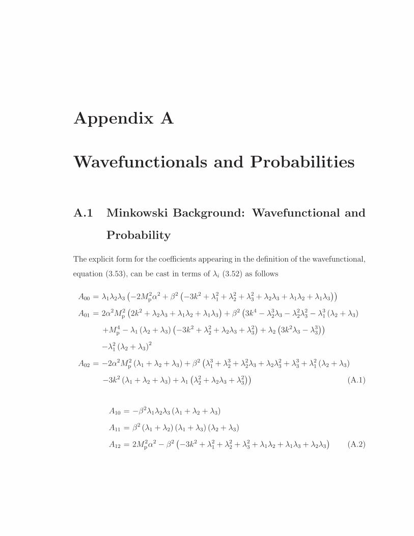
Appendix A
Wavefunctionals and Probabilities
A.1 Minkowski Background: Wavefunctional and
Probability
The explicit form for the coefficients appearing in the definition of the wavefunctional,
equation (3.53), can be cast in terms of λi (3.52) as follows
A00 = λ1λ2λ3(
−2M2pα
2 + β2(
−3k2 + λ21 + λ22 + λ23 + λ2λ3 + λ1λ2 + λ1λ3))
A01 = 2α2M2p
(
2k2 + λ2λ3 + λ1λ2 + λ1λ3)
+ β2(
3k4 − λ32λ3 − λ22λ23 − λ31 (λ2 + λ3)
+M4p − λ1 (λ2 + λ3)
(
−3k2 + λ22 + λ2λ3 + λ23)
+ λ2(
3k2λ3 − λ33))
−λ21 (λ2 + λ3)2
A02 = −2α2M2p (λ1 + λ2 + λ3) + β2
(
λ31 + λ32 + λ22λ3 + λ2λ23 + λ33 + λ21 (λ2 + λ3)
−3k2 (λ1 + λ2 + λ3) + λ1(
λ22 + λ2λ3 + λ23))
(A.1)
A10 = −β2λ1λ2λ3 (λ1 + λ2 + λ3)
A11 = β2 (λ1 + λ2) (λ1 + λ3) (λ2 + λ3)
A12 = 2M2pα
2 − β2(
−3k2 + λ21 + λ22 + λ23 + λ1λ2 + λ1λ3 + λ2λ3)
(A.2)

A.2 de Sitter Background: Classical Solutions and Probability 105
A20 = β2λ1λ2λ3
A21 = −β2 (λ2λ3 + λ1λ2 + λ1λ3)
A22 = β2 (λ1 + λ2 + λ3) . (A.3)
The traced probability in Lorentzian time then reads
P [γ0] = NN∗ exp
[
1
4M2pβ
2(λ1 + λ2 + λ3)
[
− 4β2λ1λ2λ3(λ1 + λ2 + λ3)[
−2M2pα
2
+β2(
−3k2 + λ21 + λ22 + λ2λ3 + λ23 + λ1(λ2 + λ3))]
+[
−2M2pα
2(λ1 + λ2 + λ3) + β2(
λ31 + λ32 + λ33 + λ22λ3 + λ2λ23 + λ21λ2 + λ21λ3
+λ1(λ2 + λ3)2 − 3k2(λ1 + λ2 + λ3)
)]2]
|γ0|2]
(A.4)
A.2 de Sitter Background: Classical Solutions and
Probability
The equations of motion in a de Sitter background, equation (3.57), admit solu-
tions in terms of Bessel functions. To find the general solution shown in the text,
equation (3.61), it is convenient to search for a factorization of the full sixth order
differential operator D6 defined in equation (3.58). D6 can be split into a fourth order
operator acting on a second order operator via
D6[z]γcl(z) = D4[z]D2[z]γcl(z) , (A.5)
where
D4[z] =1
z2d4
dz4−(
2
z2+
1
4z4
(
25− 4λ2i − 8M2
p
H2
α2
β2
))
d2
dz2
+1
2z5
(
25− 4λ2i − 8M2
p
H2
α2
β2
)
d
dz+
1
z2− 2
M2p
H2
α2
β2z4+
25− 4λ2i4z4
+1
16z6β2H4
[
8M4p − 8H2M2
p
(
α2 − 48Λ2 − 4α2λ2i)
+β2H4(
153− 104λ2i + 16λ4i)]
, (A.6)
D2[z] = z2d2
dz2− 2z
d
dz−(
z2 + λ2i −9
4
)
. (A.7)
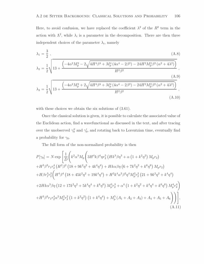
A.2 de Sitter Background: Classical Solutions and Probability 106
Here, to avoid confusion, we have replaced the coefficient λ2 of the R2 term in the
action with Λ2, while λi is a parameter in the decomposition. There are then three
independent choices of the parameter λi, namely
λ1 =3
2, (A.8)
λ2 =1
2
√
√
√
√
13 +
(
−4α2M2p − 2
√
4H4β4 +M4p (4α
4 − 2β2)− 24H2M2pβ
2 (α2 + 4λ2))
H2β2,
(A.9)
λ3 =1
2
√
√
√
√
13 +
(
−4α2M2p + 2
√
4H4β4 +M4p (4α
4 − 2β2)− 24H2M2pβ
2 (α2 + 4λ2))
H2β2,
(A.10)
with these choices we obtain the six solutions of (3.61).
Once the classical solution is given, it is possible to calculate the associated value of
the Euclidean action, find a wavefunctional as discussed in the text, and after tracing
over the unobserved γ′′0 and γ′0, and rotating back to Lorentzian time, eventually find
a probability for γ0.
The full form of the non-normalized probability is then
P [γ0] = N exp
[
1
D
(
k2α3Mp
(
3H4kβ4ηr52(
Hk3βη3 + α(
1 + k2η2)
Mpr2)
+H3β3r1r42
(
H2β2(
18 + 9k2η2 + 4k4η4)
+Hkαβη(
6 + 7k2η2 + k6η6)
Mpr2)
+Hβr31r22
(
H4β4(
18 + 45k2η2 + 19k4η4)
+H2k4α2β2η4M2pr
22
(
21 + 9k2η2 + k4η4)
+2Hkα3βη(
12 + 17k2η2 + 5k4η4 + k6η6)
M3pr
32 + α4
(
1 + k2η2 + k4η4 + k6η6)
M4pr
42
)
+H3β3r1r42α
2M2pr
22
(
1 + k2η2) (
1 + k4η4)
+M5p (A1 + A2 + A3) + A4 + A5 + A6
))]
,
(A.11)
A.2 de Sitter Background: Classical Solutions and Probability 107
where the denominator at the exponent and the Ai are given by
D = H2β2η(
1 + k2η2)
(r1 − r2)[
−H4β4r1(
3 + 2k2η2)
−H4β4r2(
3 + 2k2η2)
+α3(
1 + k2η2)
M3pr
41
(
Hβk3η3 + αMpr2(
1 + k2η2))
+Hα2βk3η3M2pr
21r2(
Hβk3η3 + αMpr2(
1 + k2η2))
+ α2M2pr
31
(
H2β2k6η6
+3Hαβk3η3Mpr2(
1 + k2η2)
+ α2M2pr
22
(
1 + k2η2)2)]
A1 = α3r81(
1 + k2η2)
(
H2β2k3η3
M2p
− Hαβr2 (2 + k2η2 + k4η4)
Mp− α2r22kη
(
1 + k2η2)
)
A2 = −α2r71
(
− H3β3k6η6
M3p
− H2αβ2k3η3r2 (12 + 17k2η2 + 3k4η4)
M2p
+Hα2βr22 (8 + 20k2η2 + 21k4η4 + 9k6η6)
Mp
+ α3kηr32(
1 + k2η2)2
)
A3 = r51
(
H5β5 (6 + 4k2η2 − 3k4η4)
M5p
− H4αβ4kηr2 (3 + 2k2η2 − 2k4η4 + k6η6)
M4p
−H3α2β3r22 (+1 + k2η2 + 2k4η4 − 10k6η6 − 4k8η8)
M3p
+ α5kηr52(
1 + k2η2)2
+H2α3β2kηr32 (18 + 39k2η2 + 26k4η4 + 5k6η6)
M2p
+2Hα4βk4η4r42 (1 + k2η2)
Mp
)
A4 = H2β2r21r32
(
H3β3(
18 + 9k2η2 + k4η4)
+Hα2βM2pr
22
(
1 + k2η2 + 5k4η4 + 2k6η6)
+H2αβ2kηMpr2(
18 + 29k2η2+ 10k4η4+ k6η6)
+ α3kηM3pr
32
(
4 + 5k2η2+ k4η4)
)
A5 = −HMpαβr61
(
3H3β3kη(
1 + k2η2)
+ α3M3pr
32
(
6 + 17k2η2 + 18k4η4 + 7k6η6)
+H2αβ2Mpr2(
1 + k2η2 + k4η4 − 12k6η6 − 4k8η8)
−Hα2βkηM2pr
22
(
−1 + 17k2η2 + 21k4η4 + k6η6)
)
A6 = r41r2
(
H5β5(
24 + 49k2η2 + 16k4η4)
+H4αβ4k3η3Mpr2(
16 + 27k2η2 + 9k4η4)
+H3α2β3k4η4M2pr
22
(
18 + 9k2η2 + k4η4)
+Hα4βM4pr
42
(
1 + k2η2) (
1 + 4k4η4)
+H2α3β2kηM3pr
32
(
39 + 57k2η2 + 20k4η4 + 4k6η6)
+ α5kηM5pr
52
(
1 + k2η2)2)
,
and where r1 and r2 are defined as
r1,2 =
√
1±√
1− β2
2α4. (A.12)
Bibliography
[1] J. A. Peacock, Cosmological Physics (1999).
[2] C. Armendariz-Picon, M. Fontanini, R. Penco, and M. Trodden, Class. Quant.
Grav. 26, 185002 (2009), 0805.0114.
[3] M. Fontanini and M. Trodden, Phys. Rev. D83, 103518 (2011), 1102.4357.
[4] M. Fontanini, E. J. West, and M. Trodden, Phys. Rev. D80, 123515 (2009),
0905.3727.
[5] A. Einstein, Annalen Phys. 49, 769 (1916).
[6] J. W. York, Physical Review Letters 28, 1082 (1972).
[7] G. W. Gibbons and S. W. Hawking, Phys. Rev. 15, 2752 (1977).
[8] S. Weinberg, The Quantum theory of fields (1995).
[9] K. Hinterbichler (2011), 1105.3735.
[10] S. N. Gupta, Phys. Rev. 96, 1683 (1954).
[11] R. H. Kraichnan, Phys. Rev. 98, 1118 (1955).
[12] S. Weinberg, Phys. Rev. 138, B988 (1965).
[13] S. Deser, Gen. Rel. Grav. 1, 9 (1970), gr-qc/0411023.
BIBLIOGRAPHY 109
[14] D. G. Boulware and S. Deser, Ann. Phys. 89, 193 (1975).
[15] J. Fang and C. Fronsdal, J. Math. Phys. 20, 2264 (1979).
[16] R. M. Wald, Phys. Rev. D33, 3613 (1986).
[17] F. A. Berends, G. J. H. Burgers, and H. Van Dam, Z. Phys. C24, 247 (1984).
[18] E. Komatsu et al. (WMAP), Astrophys. J. Suppl. 192, 18 (2011), 1001.4538.
[19] K. N. Abazajian, J. K. Adelman-McCarthy, M. A. Agueros, S. S. Allam, C. Al-
lende Prieto, D. An, K. S. J. Anderson, S. F. Anderson, J. Annis, N. A. Bahcall,
et al., Astrophys. J. Suppl. 182, 543 (2009), 0812.0649.
[20] G. Lemaitre, Gen. Rel. Grav. 29, 641 (1997).
[21] R. C. Tolman, Proc. Nat. Acad. Sci. 20, 169 (1934).
[22] H. Bondi, Mon. Not. Roy. Astron. Soc. 107, 410 (1947).
[23] D. Baumann, A. Nicolis, L. Senatore, and M. Zaldarriaga (2010), 1004.2488.
[24] E. W. Kolb, S. Matarrese, and A. Riotto, New J. Phys. 8, 322 (2006),
astro-ph/0506534.
[25] L. Boubekeur, P. Creminelli, J. Norena, and F. Vernizzi, JCAP 0808, 028
(2008), 0806.1016.
[26] T. Appelquist and J. Carazzone, Phys. Rev. D11, 2856 (1975).
[27] W. D. Goldberger (2007), hep-ph/0701129.
[28] C. P. Burgess, Ann. Rev. Nucl. Part. Sci. 57, 329 (2007), hep-th/0701053.
[29] A. Pich (1998), hep-ph/9806303.
[30] S. M. Carroll (2004), san Francisco, USA: Addison-Wesley (2004) 513 p.
BIBLIOGRAPHY 110
[31] D. Larson, J. Dunkley, G. Hinshaw, E. Komatsu, M. R. Nolta, C. L. Bennett,
B. Gold, M. Halpern, R. S. Hill, N. Jarosik, et al., Astrophys. J. Suppl. 192,
16 (2011), 1001.4635.
[32] S. Perlmutter et al. (Supernova Cosmology Project), Astrophys.J. 517, 565
(1999), the Supernova Cosmology Project, astro-ph/9812133.
[33] A. G. Riess et al. (Supernova Search Team), Astrophys. J. 607, 665 (2004),
astro-ph/0402512.
[34] P. Astier et al., Astron. Astrophys. 447, 31 (2006), astro-ph/0510447.
[35] S. M. Carroll, W. H. Press, and E. L. Turner, Ann. Rev. Astron. Astrophys.
30, 499 (1992).
[36] V. Sahni and A. A. Starobinsky, Int. J. Mod. Phys. D9, 373 (2000),
astro-ph/9904398.
[37] E. J. Copeland, M. Sami, and S. Tsujikawa, International Journal of Modern
Physics D 15, 1753 (2006), arXiv:hep-th/0603057.
[38] R. R. Caldwell, M. Kamionkowski, and N. N. Weinberg, Physical Review Letters
91, 071301 (2003), arXiv:astro-ph/0302506.
[39] T. Damour and G. Esposito-Farese, Classical and Quantum Gravity 9, 2093
(1992).
[40] T. Clifton, P. G. Ferreira, A. Padilla, and C. Skordis, ArXiv e-prints (2011),
1106.2476.
[41] S. Nojiri and S. D. Odintsov, ArXiv e-prints (2010), 1011.0544.
[42] S. M. Carroll, A. de Felice, V. Duvvuri, D. A. Easson, M. Trodden, and M. S.
Turner, Phys. Rev. D 71, 063513 (2005), arXiv:astro-ph/0410031.
BIBLIOGRAPHY 111
[43] K. Koyama, General Relativity and Gravitation 40, 421 (2008), 0706.1557.
[44] D. Bazeia, A. R. Gomes, L. Losano, and R. Menezes, Physics Letters B 671,
402 (2009), 0808.1815.
[45] J. M. Cline, J. Descheneau, M. Giovannini, and J. Vinet, Journal of High Energy
Physics 6, 48 (2003), arXiv:hep-th/0304147.
[46] F. Zwicky, Helvetica Physica Acta 6, 110 (1933).
[47] M. Milgrom, Astrophys. J. 270, 384 (1983).
[48] S. Colafrancesco, AIP Conf. Proc. 1206, 5 (2010), 1004.3869.
[49] D. H. Lyth and A. Riotto, Phys. Rept. 314, 1 (1999), hep-ph/9807278.
[50] S. Dodelson, W. H. Kinney, and E. W. Kolb, Phys. Rev. D56, 3207 (1997),
astro-ph/9702166.
[51] W. H. Kinney, E. W. Kolb, A. Melchiorri, and A. Riotto, Phys. Rev. D69,
103516 (2004), hep-ph/0305130.
[52] C. Cheung, P. Creminelli, A. Fitzpatrick, J. Kaplan, and L. Senatore, JHEP
0803, 014 (2008), 0709.0293.
[53] G. R. Dvali, G. Gabadadze, and M. Porrati, Phys. Lett. B485, 208 (2000),
hep-th/0005016.
[54] M. Ostrogradski, Mem. Acad. St. Petersburg 4, 385 (1850).
[55] A. Hindawi, B. A. Ovrut, and D. Waldram, Phys. Rev. D53, 5583 (1996),
hep-th/9509142.
[56] A. Hindawi, B. A. Ovrut, and D. Waldram, Phys. Rev. D53, 5597 (1996),
hep-th/9509147.
BIBLIOGRAPHY 112
[57] K. van Acoleyen and J. van Doorsselaere, Phys. Rev. D 83, 084025 (2011),
1102.0487.
[58] A. Nicolis, R. Rattazzi, and E. Trincherini, Phys. Rev. D79, 064036 (2009),
0811.2197.
[59] M. Trodden and K. Hinterbichler (2011), 1104.2088.
[60] A. I. Vainshtein, Phys. Lett. B39, 393 (1972).
[61] J. Lee and R. M. Wald, Journal of Mathematical Physics 31, 725 (1990).
[62] K. Andrzejewski, J. Gonera, P. Machalski, and P. Maslanka, Phys. Rev. D 82,
045008 (2010), 1005.3941.
[63] H.-J. Schmidt, Phys. Rev. D 49, 6354 (1994), arXiv:gr-qc/9404038.
[64] F. J. de Urries and J. Julve, Journal of Physics A Mathematical General 31,
6949 (1998), arXiv:hep-th/9802115.
[65] J. M. Pons, Letters in Mathematical Physics 17, 181 (1989).
[66] T. Nakamura and S. Hamamoto, Progress of Theoretical Physics 95, 469 (1996),
arXiv:hep-th/9511219.
[67] R. P. Woodard, Lect. Notes Phys. 720, 403 (2007), astro-ph/0601672.
[68] H. J. Schmidt, Class. Quant. Grav. 7, 1023 (1990).
[69] D. Wands, Class. Quant. Grav. 11, 269 (1994), gr-qc/9307034.
[70] A. A. Starobinsky, Phys. Lett. B91, 99 (1980).
[71] A. H. Guth, Phys. Rev. D23, 347 (1981).
[72] A. D. Linde, Phys. Lett. B108, 389 (1982).
BIBLIOGRAPHY 113
[73] A. Albrecht and P. J. Steinhardt, Phys. Rev. Lett. 48, 1220 (1982).
[74] V. F. Mukhanov and G. V. Chibisov, JETP Lett. 33, 532 (1981).
[75] S. W. Hawking, Phys. Lett. B115, 295 (1982).
[76] A. H. Guth and S. Y. Pi, Phys. Rev. Lett. 49, 1110 (1982).
[77] A. A. Starobinsky, Phys. Lett. B117, 175 (1982).
[78] J. M. Bardeen, P. J. Steinhardt, and M. S. Turner, Phys. Rev. D28, 679 (1983).
[79] R. H. Brandenberger (1999), hep-ph/9910410.
[80] S. Hollands and R. M. Wald, Gen.Rel.Grav. 36, 2595 (2004), 5th prize Essay,
Gravity Research Foundation, gr-qc/0405082.
[81] J. Martin and R. H. Brandenberger, Phys.Rev. D63, 123501 (2001),
hep-th/0005209.
[82] R. H. Brandenberger and J. Martin, Mod.Phys.Lett. A16, 999 (2001),
astro-ph/0005432.
[83] J. C. Niemeyer, Phys.Rev. D63, 123502 (2001), astro-ph/0005533.
[84] A. Kempf, Phys.Rev. D63, 083514 (2001), astro-ph/0009209.
[85] A. A. Starobinsky, Pisma Zh.Eksp.Teor.Fiz. 73, 415 (2001),
astro-ph/0104043.
[86] R. Easther, B. R. Greene, W. H. Kinney, and G. Shiu, Phys.Rev. D64, 103502
(2001), hep-th/0104102.
[87] R. Easther, B. R. Greene, W. H. Kinney, and G. Shiu, Phys.Rev. D67, 063508
(2003), hep-th/0110226.
BIBLIOGRAPHY 114
[88] J. C. Niemeyer and R. Parentani, Phys.Rev. D64, 101301 (2001),
astro-ph/0101451.
[89] A. Kempf and J. C. Niemeyer, Phys.Rev. D64, 103501 (2001),
astro-ph/0103225.
[90] R. H. Brandenberger and J. Martin, Int.J.Mod.Phys. A17, 3663 (2002),
hep-th/0202142.
[91] U. H. Danielsson, Phys.Rev. D66, 023511 (2002), hep-th/0203198.
[92] R. Easther, B. R. Greene, W. H. Kinney, and G. Shiu, Phys.Rev. D66, 023518
(2002), hep-th/0204129.
[93] L. Bergstrom and U. H. Danielsson, JHEP 0212, 038 (2002), hep-th/0211006.
[94] N. Kaloper, M. Kleban, A. E. Lawrence, and S. Shenker, Phys.Rev. D66,
123510 (2002), hep-th/0201158.
[95] C. Armendariz-Picon and E. A. Lim, JCAP 0312, 006 (2003), hep-th/0303103.
[96] J. Martin and R. Brandenberger, Phys.Rev. D68, 063513 (2003),
hep-th/0305161.
[97] O. Elgaroy and S. Hannestad, Phys.Rev. D68, 123513 (2003),
astro-ph/0307011.
[98] J. Martin and C. Ringeval, Phys.Rev. D69, 083515 (2004), astro-ph/0310382.
[99] T. Okamoto and E. A. Lim, Phys.Rev. D69, 083519 (2004), astro-ph/0312284.
[100] S. Shankaranarayanan and L. Sriramkumar, Phys.Rev. D70, 123520 (2004),
hep-th/0403236.
[101] J. Martin and C. Ringeval, JCAP 0501, 007 (2005), hep-ph/0405249.
BIBLIOGRAPHY 115
[102] K. Schalm, G. Shiu, and J. P. van der Schaar, JHEP 0404, 076 (2004),
hep-th/0401164.
[103] B. R. Greene, K. Schalm, G. Shiu, and J. P. van der Schaar, JCAP 0502, 001
(2005), hep-th/0411217.
[104] K. Schalm, G. Shiu, and J. P. van der Schaar, AIP Conf.Proc. 743, 362 (2005),
hep-th/0412288.
[105] R. Easther, W. H. Kinney, and H. Peiris, JCAP 0505, 009 (2005),
astro-ph/0412613.
[106] B. Greene, K. Schalm, J. P. van der Schaar, and G. Shiu, p. 0001 (2004),
astro-ph/0503458.
[107] A. Kempf and L. Lorenz, Phys.Rev. D74, 103517 (2006), gr-qc/0609123.
[108] R. Holman and A. J. Tolley, JCAP 0805, 001 (2008), 0710.1302.
[109] S. Weinberg, Phys.Rev. D77, 123541 (2008), 0804.4291.
[110] B. Losic and W. Unruh, Phys.Rev.Lett. 101, 111101 (2008), 0804.4296.
[111] W. Hu (2004), astro-ph/0402060.
[112] V. F. Mukhanov, Sov. Phys. JETP 67, 1297 (1988).
[113] S. Weinberg, Phys.Rev. D72, 043514 (2005), hep-th/0506236.
[114] J. F. Donoghue, Phys.Rev. D50, 3874 (1994), gr-qc/9405057.
[115] D. Spergel et al. (WMAP Collaboration), Astrophys.J.Suppl. 170, 377 (2007),
astro-ph/0603449.
[116] C. Armendariz-Picon, JCAP 0702, 031 (2007), astro-ph/0612288.
BIBLIOGRAPHY 116
[117] N. Arkani-Hamed, H.-C. Cheng, M. A. Luty, and S. Mukohyama, JHEP 0405,
074 (2004), hep-th/0312099.
[118] N. Arkani-Hamed, P. Creminelli, S. Mukohyama, and M. Zaldarriaga, JCAP
0404, 001 (2004), hep-th/0312100.
[119] F. Piazza and S. Tsujikawa, JCAP 0407, 004 (2004), hep-th/0405054.
[120] T. Chiba, JCAP 0503, 008 (2005), gr-qc/0502070.
[121] G. Calcagni, B. de Carlos, and A. De Felice, Nucl.Phys. B752, 404 (2006),
hep-th/0604201.
[122] C. de Rham and A. J. Tolley, JCAP 0607, 004 (2006), hep-th/0605122.
[123] K. Koyama, Class.Quant.Grav. 24, R231 (2007), 0709.2399.
[124] P. D. Mannheim (2011), 1101.2186.
[125] C. M. Bender and P. D. Mannheim, J.Phys.A 41, 304018 (2008), * Temporary
entry *, 0807.2607.
[126] S. Hawking and T. Hertog, Phys.Rev. D65, 103515 (2002), hep-th/0107088.
[127] T. Clunan and M. Sasaki, Class.Quant.Grav. 27, 165014 (2010), 0907.3868.
[128] R. Di Criscienzo and S. Zerbini, J.Math.Phys. 50, 103517 (2009), 0907.4265.
[129] R. Forman, Inventiones Mathematicae 88, 447 (1987).
[130] I. M. Gel’Fand and A. M. Yaglom, Journal of Mathematical Physics 1, 48
(1960).
[131] S. Levit and U. Smilansky, Proc. Amer. Math. Soc. 65, 299 (1977).
[132] A. G. Riess et al. (Supernova Search Team), Astron.J. 116, 1009 (1998),
astro-ph/9805201.
BIBLIOGRAPHY 117
[133] N. A. Bahcall, J. P. Ostriker, S. Perlmutter, and P. J. Steinhardt, Science 284,
1481 (1999), astro-ph/9906463.
[134] P. Peebles and B. Ratra, Rev.Mod.Phys. 75, 559 (2003), astro-ph/0207347.
[135] E. J. Copeland, M. Sami, and S. Tsujikawa, Int.J.Mod.Phys. D15, 1753 (2006),
hep-th/0603057.
[136] J. Frieman, M. Turner, and D. Huterer, Ann.Rev.Astron.Astrophys. 46, 385
(2008), 0803.0982.
[137] R. R. Caldwell and M. Kamionkowski, Ann.Rev.Nucl.Part.Sci. 59, 397 (2009),
* Brief entry *, 0903.0866.
[138] A. Silvestri and M. Trodden, Rept.Prog.Phys. 72, 096901 (2009), * Brief entry
*, 0904.0024.
[139] K. Tomita, Mon.Not.Roy.Astron.Soc. 326, 287 (2001), * Brief entry *,
astro-ph/0011484.
[140] K. Tomita, Prog.Theor.Phys. 106, 929 (2001), astro-ph/0104141.
[141] K. Tomita, Prog.Theor.Phys. 108, 103 (2002), astro-ph/0203125.
[142] J. W. Moffat, JCAP 0510, 012 (2005), astro-ph/0502110.
[143] H. Alnes, M. Amarzguioui, and O. Gron, Phys.Rev. D73, 083519 (2006),
astro-ph/0512006.
[144] K. T. Inoue and J. Silk, Astrophys.J. 648, 23 (2006), astro-ph/0602478.
[145] K. T. Inoue and J. Silk, Astrophys.J. 664, 650 (2007), astro-ph/0612347.
[146] D. J. Chung and A. E. Romano, Phys.Rev. D74, 103507 (2006), * Brief entry
*, astro-ph/0608403.
BIBLIOGRAPHY 118
[147] H. Alnes and M. Amarzguioui, Phys.Rev. D74, 103520 (2006),
astro-ph/0607334.
[148] J. Garcia-Bellido and T. Haugboelle, JCAP 0804, 003 (2008), * Brief entry *,
0802.1523.
[149] J. Garcia-Bellido and T. Haugboelle, JCAP 0809, 016 (2008), * Brief entry *,
0807.1326.
[150] J. Garcia-Bellido and T. Haugboelle, JCAP 0909, 028 (2009), * Brief entry *,
0810.4939.
[151] J. Zibin, A. Moss, and D. Scott, Phys.Rev.Lett. 101, 251303 (2008), 0809.3761.
[152] C. Quercellini, M. Quartin, and L. Amendola, Phys.Rev.Lett. 102, 151302
(2009), 0809.3675.
[153] M. Perryman, K. S. de Boer, G. Gilmore, E. Hog, M. Lattanzi, et al., As-
tron.Astrophys. 369, 339 (2001), * Brief entry *, astro-ph/0101235.
[154] S. Kanno, M. Kimura, J. Soda, and S. Yokoyama, JCAP 0808, 034 (2008),
0806.2422.
[155] M.-a. Watanabe, S. Kanno, and J. Soda, Phys.Rev.Lett. 102, 191302 (2009),
0902.2833.
[156] S. Yokoyama and J. Soda, JCAP 0808, 005 (2008), * Brief entry *, 0805.4265.
[157] L. Ackerman, S. M. Carroll, and M. B. Wise, Phys.Rev. D75, 083502 (2007),
astro-ph/0701357.
[158] T. Jaffe, A. Banday, H. Eriksen, K. Gorski, and F. Hansen, Astrophys.J. 629,
L1 (2005), astro-ph/0503213.

BIBLIOGRAPHY 119
[159] T. Jaffe, A. Banday, H. Eriksen, K. Gorski, and F. Hansen, Astron.Astrophys.
460, 393 (2006), astro-ph/0606046.
[160] L. Campanelli, P. Cea, and L. Tedesco, Phys.Rev.Lett. 97, 131302 (2006),
astro-ph/0606266.
[161] L. Campanelli, P. Cea, and L. Tedesco, Phys.Rev. D76, 063007 (2007),
0706.3802.
[162] B. Himmetoglu, C. R. Contaldi, and M. Peloso, Phys.Rev.Lett. 102, 111301
(2009), 0809.2779.
[163] C. Armendariz-Picon, JCAP 0407, 007 (2004), astro-ph/0405267.
[164] T. Koivisto and D. F. Mota, JCAP 0806, 018 (2008), * Brief entry *,
0801.3676.
[165] W. Freedman et al. (HST Collaboration), Astrophys.J. 553, 47 (2001),
astro-ph/0012376.
[166] A. G. Riess, L. Macri, S. Casertano, M. Sosey, H. Lampeitl, et al., Astrophys.J.
699, 539 (2009), * Brief entry *, 0905.0695.
[167] G. F. R. Ellis and M. A. H. MacCallum, Commun. Math. Phys. 12, 108 (1969).
[168] L. D. Landau and E. M. Lifshitz, The classical theory of fields (1975).
[169] J. D. Barrow, Phys.Rev. D55, 7451 (1997), gr-qc/9701038.
[170] G. Hinshaw et al. (WMAP Collaboration), Astrophys.J.Suppl. 180, 225 (2009),
0803.0732.
[171] F. Ding and R. A. Croft (2009), * Brief entry *, 0903.3402.

Biographical Information
NAME OF AUTHOR: Michele Fontanini
PLACE OF BIRTH: Udine, UD, Italy
DATE OF BIRTH: March 9, 1979
GRADUATE AND UNDERGRADUATE SCHOOLS ATTENDED:
Universita degli Studi di Trieste, Trieste, Italy
Syracuse University, Syracuse, New York
DEGREES AWARDED:
Bachelor of Science in Physics, 2001, Universita degli Studi di Trieste
Masters of Science in Theoretical Physics, 2005, Universita degli Studi di Trieste
PROFESSIONAL EXPERIENCE:
Teaching Assistant, Department of Physics, Syracuse University, 2006-2008
Instructor, Department of Physics, Syracuse University, Summer 2007