J. Parallel Distrib. Comput. 63 (2003) 1164–1172

ARTICLE IN PRESS

�Corresp

E-mail

julio@uxde

(I. Stojmen

0743-7315/$

doi:10.1016

Higher dimensional hexagonal networks

Fabian Garcıa,a Julio Solano,a Ivan Stojmenovic,b,� and Milos Stojmenovicb

aDISCA, IIMAS, UNAM, Circuito Escolar S/N, Ciudad Universitaria, Coyoacan, Mexico City 04510, MexicobDeptartment of Computer Science, University of Ottawa, SITE, 550 Cumberland St., Ottawa, ON, Canada K1N 6N5

Received 11 February 2003; revised 18 June 2003

Abstract

We define the higher dimensional hexagonal graphs as the generalization of a triangular plane tessellation, and consider it as a

multiprocessor interconnection network. Nodes in a k-dimensional (k-D) hexagonal network are placed at the vertices of a k-D

triangular tessellation, so that each node has up to 2k þ 2 neighbors. In this paper, we propose a simple addressing scheme for the

nodes, which leads to a straightforward formula for computing the distance between nodes and a very simple and elegant routing

algorithm. The number of shortest paths between any two nodes and their description are also provided in this paper. We then

derive closed formulas for the surface area (volume) of these networks, which are defined as the number of nodes located at a given

distance (up to a given distance, respectively) from the origin node. The number of nodes and the network diameter under a more

symmetrical border conditions are also derived. We show that a k-D hexagonal network of size t has the same degree, the same or

lower diameter, and fewer nodes than a ðk þ 1Þ-D mesh of size t. Simple embeddings between two networks are also described. That

is, we show how to reduce the dimension of a mesh by removing some nodes, and converting it into a hexagonal network, while

preserving the simplicity of basic data communication schemes such as routing and broadcasting.

r 2003 Elsevier Inc. All rights reserved.

Keywords: Interconnection networks; Hexagonal networks; Addressing; Routing

1. Introduction

Direct interconnection networks can be modeled bygraphs, with nodes and edges corresponding to proces-sors and communication links between them, respec-tively. A survey of these networks is given in [23]. Thispaper proposes a new direct interconnection networkmodel. It also studies addressing and routing schemesfor some topological properties of the new model, suchas: degree (maximal number of edges from a node), nodeand edge symmetry and surface area (defined as thenumber of nodes at a given distance from the originnode).There exist three regular plane tessellations, com-

posed of the same kind of regular (equilateral) polygons:triangular, square, and hexagonal. They are the basis forthe designs of direct interconnection networks withhighly competitive overall performance. Mesh con-

onding author. www.site.uottowa.ca/Bivan.

addresses: fabian@uxdea4.iimas.unam.mx (F. Garcıa),

a4.iimas.unam.mx (J. Solano), ivan@site.uottawa.ca

ovic).

- see front matter r 2003 Elsevier Inc. All rights reserved.

/j.jpdc.2003.07.001

nected computers and tori (tori are meshes with addedlinks between the first and the last processor in any rowor column, that is, in any direction for the higherdimensional case) are based on regular square tessella-tions, and are popular and well-known models forparallel processing. Their extension, the m-ary k-cube,has been used as the underlying topology for mostpractical multicomputers (e.g. J-machine [17], iWarp[19], Ncube-2 [16], Cray T3E [1] and Cray T3D [12]),and has been extensively studied in the literature. Thetopological properties and routing algorithms for the m-ary k-cubes have been extensively studied in the past[10]. An expression for the surface area of a t-ary k-cubeis provided in [2,3].Hexagonal and honeycomb networks are based on

regular triangular and hexagonal tessellations, respec-tively. The inconsistency in the name selection (note thata hexagonal network is not based on a hexagon, but ona triangular tessellation) is due to the duality of the twotessellations (one can be obtained from the other byjoining the centers of the neighboring polygons) and thename selection taken in the past, which other authorskept afterwards.

ARTICLE IN PRESS

k

i

j

x

y

z

(0 ,0 ,0 )

(-1,0,0)=(0,1,1)(-1,0,2) (-1,0,1)

(0,-2,1)

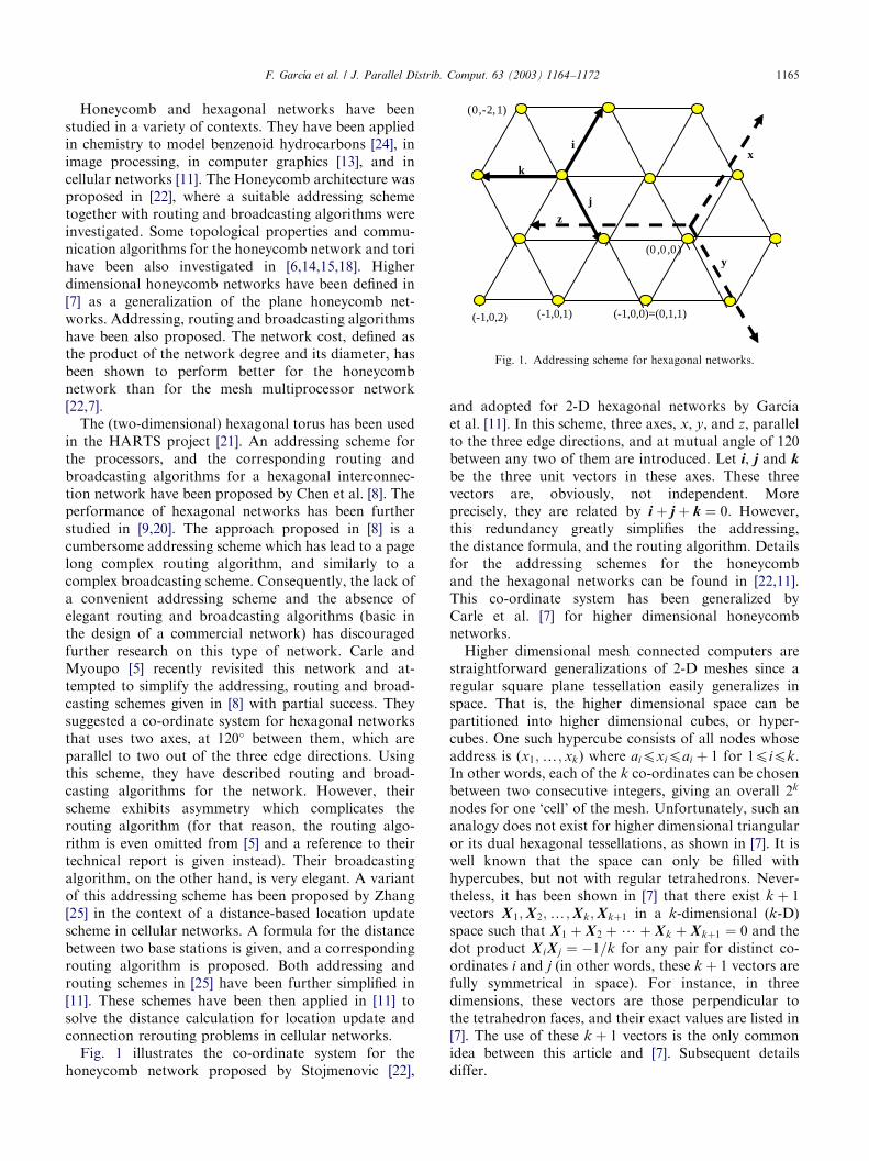
Fig. 1. Addressing scheme for hexagonal networks.

F. Garc!ıa et al. / J. Parallel Distrib. Comput. 63 (2003) 1164–1172 1165

Honeycomb and hexagonal networks have beenstudied in a variety of contexts. They have been appliedin chemistry to model benzenoid hydrocarbons [24], inimage processing, in computer graphics [13], and incellular networks [11]. The Honeycomb architecture wasproposed in [22], where a suitable addressing schemetogether with routing and broadcasting algorithms wereinvestigated. Some topological properties and commu-nication algorithms for the honeycomb network and torihave been also investigated in [6,14,15,18]. Higherdimensional honeycomb networks have been defined in[7] as a generalization of the plane honeycomb net-works. Addressing, routing and broadcasting algorithmshave been also proposed. The network cost, defined asthe product of the network degree and its diameter, hasbeen shown to perform better for the honeycombnetwork than for the mesh multiprocessor network[22,7].The (two-dimensional) hexagonal torus has been used

in the HARTS project [21]. An addressing scheme forthe processors, and the corresponding routing andbroadcasting algorithms for a hexagonal interconnec-tion network have been proposed by Chen et al. [8]. Theperformance of hexagonal networks has been furtherstudied in [9,20]. The approach proposed in [8] is acumbersome addressing scheme which has lead to a pagelong complex routing algorithm, and similarly to acomplex broadcasting scheme. Consequently, the lack ofa convenient addressing scheme and the absence ofelegant routing and broadcasting algorithms (basic inthe design of a commercial network) has discouragedfurther research on this type of network. Carle andMyoupo [5] recently revisited this network and at-tempted to simplify the addressing, routing and broad-casting schemes given in [8] with partial success. Theysuggested a co-ordinate system for hexagonal networksthat uses two axes, at 120� between them, which areparallel to two out of the three edge directions. Usingthis scheme, they have described routing and broad-casting algorithms for the network. However, theirscheme exhibits asymmetry which complicates therouting algorithm (for that reason, the routing algo-rithm is even omitted from [5] and a reference to theirtechnical report is given instead). Their broadcastingalgorithm, on the other hand, is very elegant. A variantof this addressing scheme has been proposed by Zhang[25] in the context of a distance-based location updatescheme in cellular networks. A formula for the distancebetween two base stations is given, and a correspondingrouting algorithm is proposed. Both addressing androuting schemes in [25] have been further simplified in[11]. These schemes have been then applied in [11] tosolve the distance calculation for location update andconnection rerouting problems in cellular networks.Fig. 1 illustrates the co-ordinate system for the

honeycomb network proposed by Stojmenovic [22],

and adopted for 2-D hexagonal networks by Garcıaet al. [11]. In this scheme, three axes, x, y, and z, parallelto the three edge directions, and at mutual angle of 120between any two of them are introduced. Let i, j and kbe the three unit vectors in these axes. These threevectors are, obviously, not independent. Moreprecisely, they are related by i þ j þ k ¼ 0: However,this redundancy greatly simplifies the addressing,the distance formula, and the routing algorithm. Detailsfor the addressing schemes for the honeycomband the hexagonal networks can be found in [22,11].This co-ordinate system has been generalized byCarle et al. [7] for higher dimensional honeycombnetworks.Higher dimensional mesh connected computers are

straightforward generalizations of 2-D meshes since aregular square plane tessellation easily generalizes inspace. That is, the higher dimensional space can bepartitioned into higher dimensional cubes, or hyper-cubes. One such hypercube consists of all nodes whoseaddress is (x1;y; xk) where aipxipai þ 1 for 1pipk:In other words, each of the k co-ordinates can be chosenbetween two consecutive integers, giving an overall 2k

nodes for one ‘cell’ of the mesh. Unfortunately, such ananalogy does not exist for higher dimensional triangularor its dual hexagonal tessellations, as shown in [7]. It iswell known that the space can only be filled withhypercubes, but not with regular tetrahedrons. Never-theless, it has been shown in [7] that there exist k þ 1vectors X1;X2;y;Xk;Xkþ1 in a k-dimensional (k-D)space such that X1 þ X2 þ?þ Xk þ Xkþ1 ¼ 0 and thedot product X iX j ¼ �1=k for any pair for distinct co-ordinates i and j (in other words, these k þ 1 vectors arefully symmetrical in space). For instance, in threedimensions, these vectors are those perpendicular tothe tetrahedron faces, and their exact values are listed in[7]. The use of these k þ 1 vectors is the only commonidea between this article and [7]. Subsequent detailsdiffer.

ARTICLE IN PRESSF. Garc!ıa et al. / J. Parallel Distrib. Comput. 63 (2003) 1164–11721166

Carle and Myoupo [5] defined a 3-D hexagonal graphas a generalization of the hexagonal network in a plane.Carle [4] further generalized the network for higherdimensions. Each node in a k-D hexagonal graph isdefined in [5,4] as the node with integer co-ordinates(x1;y;xk). The network has two kinds of edges. Twonodes (x1;y; xk) and (x0

1;y; x0k) are connected by an

edge if their addresses differ by one in exactly onedirection, that is, |x1 � x0

1|+?+|xk � x0k|=1. Therefore,

higher dimensional meshes are sub-graphs of higherdimensional hexagons, as defined in [5,4] (with networkborders being defined in a different manner). Somediagonal edges are added to the network as follows. Twonodes are connected by an edge when there exist exactlytwo co-ordinates i and j such that ðxi � x0

iÞðxj � x0jÞ ¼ 1

(the product is otherwise equal to 0). Therefore, eachnode has kðk � 1Þ=2 diagonal edges. The overall numberof edges at each node (that is, the network degree) istherefore quadratic with the network dimension, asopposed to being linear for higher dimensional meshesand honeycombs. This is a significant drawback for theproposed generalization [4,5]. Moreover, no formulafor the distance between two nodes in the networkhas been given in [4,5], and the routing scheme offered isnot shown to follow the shortest path between twonodes. Clearly, an adapted routing scheme shouldfollow the shortest path between any two nodes.The addressing scheme proposed in [4,5] for thenetwork is therefore sophisticated, has an excessivedegree, and is discouraging for further study of thenetwork.In this paper, we suggest a variation for the general-

ization of the plane hexagonal graph to a higherdimensional hexagonal network. This new generaliza-tion presents a linear degree (more precisely, 2k þ 2) andhas a very simple addressing scheme, which leads to astraightforward formula for the distance between twonodes and to a straightforward routing algorithm, notonly for one shortest path but also for all the shortestpaths. Further, it allows to count and list the number ofshortest paths between two nodes and to count thenumber of nodes at a given distance from a given node(that is, to find a closed formula for the surface area ofthe network). Thus, this new generalization will beshown to be a viable alternative to the well-knownhigher dimensional mesh connected computer,and the higher dimensional honeycomb network.We will also show embeddings and analogies betweenthe two networks, and a simple broadcastingalgorithm for the hexagonal networks. The proposednetwork can be physically implemented with existingtechnology like any other interconnection network,with processors replacing nodes and communicationlinks added between processors according to thegraph definition of higher dimensional hexagonalnetwork.

2. An addressing scheme for higher dimensional

hexagonal networks

The goal of this paper is to describe a higherdimensional hexagonal network as a generalization of2-D one, preserving desirable properties such as lowdiameter, small degree and symmetries. We observethat, starting from an origin node, all nodes of a 2-Dhexagonal network are obtained by adding unit sizevectors along three symmetrically positioned directionsin the plane. We will therefore extend this constructionto k-D space. Starting from the origin, unit size vectorswill be added and will lead to new nodes along k þ 1symmetrically positioned vectors (in both positive ornegative orientations along these vectors), so that eachnode has at most 2k þ 2 neighbors. Two nodes areneighbors in such graph if and only if they differ by oneof such 2k þ 2 unit size vectors (in vector sense). Whilesuch construction is intuitively clear, the addressing ofnodes in such networks is not obvious. Our maincontribution is to propose a co-ordinate system that canbe used to assign ids to the nodes in a higherdimensional hexagonal network. We will then showthat the distance between any two nodes can becomputed easily if the proposed node id assignmentscheme is utilized. Let X1;X2;y;Xk;Xkþ1 be k þ 1(unit) vectors in a k-D space such that X1 þ X2 þ?þXk þ Xkþ1 ¼ 0 (the dot product property is not neededin the sequel). The nodes in a k-D hexagonal networkcan be defined as follows.

Definition 1. Choose any node as the origin and assign(0; 0;y; 0) (k þ 1 zeros) as its address. For any othernode A on the network, if there is a path from the originto node A, and the path has altogether |ai| units ofvector sign(ai)X i (that is, X i for ai 40 and –X i

otherwise), 1pipk þ 1; then an address for node A isða1;y; akþ1Þ ¼ a1x1 þ?þ Akþ1Xkþ1:

Clearly, more than one ðk þ 1Þ-tuple point corre-sponds to the same node. For example, in Fig. 1,(�1,0,0)=(0,1,1) since –i=j+k and thus the twopaths, the direct one, and using the two other sidesof the equilateral triangle, end in the same point.In general, we have ða1;y; akþ1Þ ¼ ða0

1;y; a0kþ1Þ

3a1X1 þ?þ akþ1Xkþ1 ¼ a01X1 þ?þ a0

kþ1Xkþ1: Inparticular, if (a1;y; akþ1)=(a0

1;y; a0kþ1), then there

exists an integer r such that a0i ¼ ai þ r; 1pipk þ 1:

Combining those two facts, we have the following. If(a1;y; akþ1) is an address for node A, then allpossible addresses for node A are of the form(a1 þ r;y; akþ1 þ r) for any integer r. Starting fromthe nonunique addressing, we shall now find a way toarrive at a unique node address. We will first define theshortest path form for the address, and then will

ARTICLE IN PRESSF. Garc!ıa et al. / J. Parallel Distrib. Comput. 63 (2003) 1164–1172 1167

define the distinguished shortest path form for thenode address.

Definition 2. An address (a1;y; akþ1) for node A is ofthe shortest path form if there is a path from the originto node A, consisting of |ai| units of either vector X i; (forai40) or vector �X i (for aio0), 1pipk þ 1; and thepath has the shortest possible length.

Corollary 1. The distance between two nodes A and B,

isja1j þ?þ jakþ1j; where B � A ¼ ða1;y; akþ1Þ is in

the shortest path form. Therefore the shortest path form

ða1;y; akþ1Þ minimizes ja1j þ?þ jakþ1j:

We shall now investigate the uniqueness of theshortest path form. Let np, nn, and nz denote thenumber of positive, negative and zero co-ordinates in ashortest path form ða1;y; akþ1Þ; respectively. Clearlynp þ nn þ nz ¼ k þ 1:

Theorem 1. If k is an even number then ða1;y; akþ1Þ is in

a shortest path form if and only if nzX1, nppk=2,

nnpk=2. The shortest path form is also the unique

shortest path form. The number of shortest paths

between two nodes A and B with B � A ¼ ða1;y; akþ1Þin the shortest path form is ðja1j þ?þ jakþ1jÞ!=ðja1j!yjakþ1j!Þ:

Proof. We will prove the theorem by contradiction.Assume that ða1;y; akþ1Þ is in a shortest path form, andnp4k=2: Without loss of generality, we assume thatai40; 1pipnp: Since a1X1 þ?þ akþ1Xkþ1 ¼ a1X1þ?þ akþ1Xkþ1–ðX1 þ?þ Xkþ1Þ ¼ ða1 � 1ÞX1 þ?þðakþ1 � 1ÞXkþ1; ða1 � 1;y; akþ1 � 1Þ is another addressfor node A. The length of the path corresponding to(a1 � 1;y; akþ1 � 1) is ja1 � 1j þ?þ jakþ1 � 1jpja1j�1þ?þ janpj � 1þ janpþ1j þ 1þ?þ jakþ1j þ 1¼ja1j þ?þ jakþ1j�np þ ðk þ 1� npÞoja1j þ?þ jakþ1jsince k þ 1o2np: It means that the path correspondingto (a1 � 1;y; akþ1 � 1) is shorter than the shortest path,a contradiction. Therefore we proved that nppk=2; andsimilarly nnpk=2: Then nz ¼ k þ 1� np � nnXk þ 1�2k=2 ¼ 1: Assume now that nzX1; nppk=2; nnpk=2 issatisfied. Then for node (a1 þ r;y; akþ1 þ r) and r40(the proof for ro0 is similar) we get ja1 þ rjþ ?þjakþ1 þ rjXja1j þ?þjakþ1j þ rðnp þ nz�nnÞ4ja1j þ?þjakþ1j(since np þ nz � nn ¼ k þ 1� 2nn40), thus (a1þr;y; akþ1 þ r) is not in the shortest path form. &

However, the shortest path form is not always uniquefor k odd. For example, for k ¼ 3; (4,4,0,0)=(3,3,�1,�1)=(2,2,�2,�2)=(1,1,�3,�3)=(0,0,�4,�4), andall these representations have the shortestpath length 8. Using similar arguments as in theproof of Theorem 1, we can prove the followingcorollaries.

Corollary 2. A node address ða1;y; akþ1Þ is in the

shortest path form if and only if nppðk þ 1Þ=2 and

nnpðk þ 1Þ=2. This is valid for both cases of k being an

odd or an even number.

Corollary 3. If k is an odd number then a shortest path

form ða1;y; akþ1Þ is unique if and only if nz4jnp � nnj.

We shall now define the median for an addressða1;y; akþ1Þ (not necessarily in the shortest path form).Let ðb1;y; bkþ1Þ be the permutation of elementsða1;y; akþ1Þ in sorted order, that is b1p?pbkþ1:The median is any integer m which satisfiesbðkþ1Þ=2pmpbðkþ1Þ=2þ1: If ða1;y; akþ1Þ is in the shortestpath form then an alternative definition of median canbe given as follows. Let mn and mp be the maximalnegative and minimal positive elements of sequenceða1;y; akþ1Þ; respectively; if there are less than ðk þ1Þ=2 negative (positive) elements then mn (mp, respec-tively) is set to 0. The median is any integer m whichsatisfies mnpmpmp.

Corollary 4. If ða1;y; akþ1Þ is an address for node A

then ða1 � m;y; akþ1 � mÞ is an address for node A in a

shortest path form for any median m.

Corollary 5. The number of shortest paths between two

nodes A and B with B � A ¼ ða1;y; akþ1Þ in a shortest

path form isPmp

m¼mnðja1 � mj þ?þ jakþ1 � mjÞ!=ðja1 �mj!yjakþ1 � mj!Þ:

Theorem 2. The address of each node can be uniquelyrepresented in the distinguished shortest path form

ða1;y; akþ1Þ; where nppIðk þ 1Þ=2m; nnpIk=2m;and nzX1:

Proof. For k even the theorem is equivalent to Theorem1. If k is odd then Corollary 4 can be applied for m=mn,leading to a (unique) distinguished shortest pathrepresentation. &

3. Routing in higher dimensional hexagonal networks

We shall now describe a corresponding routingalgorithm from a source S to a destination D, whereD � S ¼ ða1;y; akþ1Þ is in a shortest path form. Thealgorithm reduces the path length at each step. Therouting algorithm is quite simple and can be described asfollows:

Algorithm route(S;D) (�D � S ¼ ða1;y; akþ1Þ is in ashortest path form �) {

For i ¼ 1 to k þ 1 do

For j ¼ 1 to |ai| do Send message |ai| times indirection sign(ai) X i }

ARTICLE IN PRESS

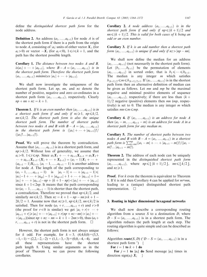
able 1

urface area of a k-D hexagonal network at distance n

n

1 2 3 4 5 6 7

2 2 2 2 2 2 2

6 12 18 24 30 36 42

8 26 56 98 152 218 296

10 50 150 340 650 1110 1750

12 72 272 762 1752 3512 6372

14 98 462 1596 4410 10,374 21,658

16 128 680 2722 8679 23,331 55,073

18 162 978 4482 16,470 50,718 135,702

20 200 1340 6800 27,752 94,940 281,360

F. Garc!ıa et al. / J. Parallel Distrib. Comput. 63 (2003) 1164–11721168

The algorithm may be easily modified to offerflexibility in selecting one of the possible shortest paths,whose number is given in Corollary 5. At each step, themessage can be sent along any edge that will shorten thedestination distance. These edges are easy to detect.Such flexible routing is important in case of congestionin a corresponding interconnection network. The levelof congestion at each node corresponds to the amountof traffic at that node (for instance, the queue length ininterconnection networks). Various heuristics for select-ing a path based on the network conditions can bederived from the analysis of congestion, but this isbeyond the scope of this paper. Note that the algorithmassumes the availability of intermediate nodes in thenetwork. Given some boundary conditions for thenodes, the algorithm might need to be modified toavoid missing nodes.

4. The surface area of higher dimensional hexagonal

networks

We shall now count the number of nodes at a givendistance n from the origin node (0,y,0). Because of thesymmetry, the same number is obtained from any node,subject to the network border conditions that can reducethe count. The surface area at distance n is equal to thenumber of nodes ða1;y; akþ1Þ in the unique shortestpath representation which satisfy ja1j þ?þ jakþ1j ¼ n

(Corollary 1). Let Cðp; qÞ ¼ p!=ðq!ðp � qÞ!Þ be thebinomial coefficient. In order to make the expressionclearer, let np max ¼ minðk þ 1� nz;Iðk þ 1Þ=2mÞ andnp min ¼ maxð0;Iðk þ 3Þ=2m� nzÞ:

Theorem 3. The surface area of a k-D hexagonal network

at distance n is

Xk

nz¼1fCðk þ 1; nzÞCðn � 1; k � nzÞ

�Xnpmax

np¼npmin

Cðk þ 1� nz; npÞg:

Proof. The number of elements nz in sequenceða1;y; akþ1Þ which are equal to zero can be between 1and k, according to Theorem 2, and the count isconsidered separately for each possible value of nz.There are Cðk þ 1; nzÞ ways to choose nz zero positionsin vector ða1;y; akþ1Þ: The remaining elements in thevector area0. Integer compositions of n into s parts arerepresentations of n as sums of s positive integers, calledparts; that is, n ¼ u1 þ?þ us; ui40; 1pips: It iswell-known that the number of such compositions isCðn � 1; s � 1Þ: In our case s ¼ k þ 1� nz: Each ofthese nonzero parts can be either a positive or a negativenumber, and the numbers np and nn of the positive and

T

S

k

1

2

3

4

5

6

7

8

9

negative numbers must be chosen in accordance toTheorem 2. Since nn ¼ k þ 1� np � nz; it suffices tofind the bounds for np. It is bounded above byboth k þ 1� nz and Iðk þ 1Þ=2mÞ; thus itsmaximum is npmax=min(k þ 1� nz;Iðk þ 1Þ=2m).Since nnpIk=2m; it follows that np ¼ k þ 1� nz �npXk þ 1� nz � Ik=2m ¼ Iðk þ 3Þ=2m� nz: It is alsobounded below by 0, therefore npmin=max(0;Iðk þ 3Þ=2m� nz). Among k þ 1� nz nonzero parts,np parts are selected to be positive, others are negative.The theorem then follows. &

Table 1 gives the surface areas of k-D hexagonalnetworks at distance n for small values of k and n. Thevolume of the network can be then calculated as thesummation over distances up to n, applied on formula inTheorem 3. The network can be bounded using themaximum distance n from the origin as a criterion for anode to belong to the network. The diameter of thenetwork is obviously 2n; which is the distance betweennodes (n; 0;y; 0) and (�n; 0;y; 0). The network degree2k þ 2 and diameter 2n can be considered as a functionof the volume, and be compared with similar analysisfor the honeycomb and mesh connected computers, inorder to compare network costs. The closed formulasfor comparison seem difficult to obtain, so one can relyon computer data to compare small size networks andderive conclusions.

5. A border with better connectivity

A k-D hexagonal network can be defined with theorigin as a center and with all nodes up to certaindistance from the origin as part of the network.However, using such border definitions, some nodeshave only one neighbor. For example, node (n; 0;y; 0)is connected only to node (n � 1; 0;y; 0) (for k42). Weshall define now a ‘friendlier’ border condition. Let a k-

ARTICLE IN PRESS

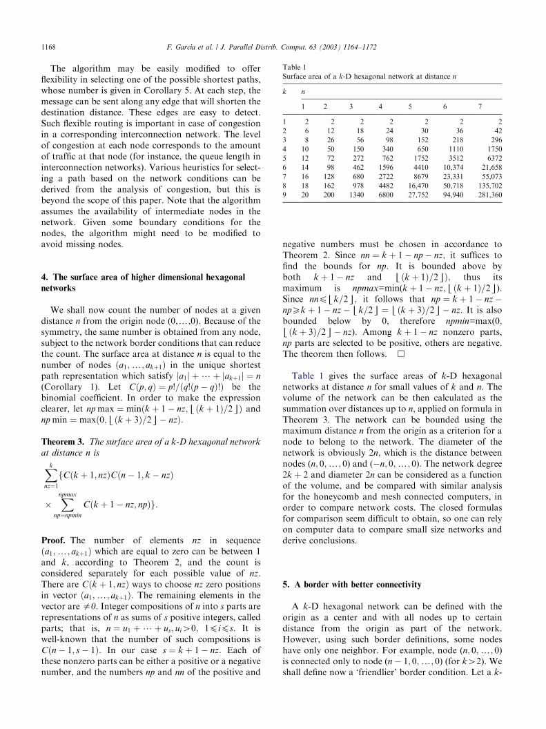
Table 2

Volume of k-D hexagonal networks of size t

k t

1 2 3 4 5 6

1 3 5 7 9 11 13

2 13 37 73 121 181 253

3 39 185 511 1089 1991 3289

4 141 1141 4441 12,201 27,301 53,341

5 423 5705 31,087 109,809 300,311 693,433

6 1429 32,845 252,169 1.1E6 3.8E6 1.0E7

7 4254 163,361 1.7E6 1.0E7 4.2E7 1.3E8

8 13,981 911,845 1.4E7 1.0E8 5.2E8 2.0E9

9 41,898 4.5E6 9.6E7 9.3E8 5.7E9 2.6E10

1100 11-10 000-1 001-1

010-1 100-1

110-1

101-1 011-1

F. Garc!ıa et al. / J. Parallel Distrib. Comput. 63 (2003) 1164–1172 1169

D hexagonal network of size t be defined as the set ofnodes whose unique shortest path form (a1;y; akþ1)satisfies jaijpt; 1pipk þ 1:

Theorem 4. The diameter of a k-D hexagonal network of

size t is 4tIðk þ 1Þ=2m:

Proof. The distance between nodes (�t;y;�t; t;y; t)and (t;y; t; �t;y;�t) (with Iðk þ 1Þ=2m positiveand negative parts in each, and with an additionalcomponent equal to 0 at the end of both for k

even) is 4tIðk þ 1Þ=2m: The distance cannot belarger since for the k even X1 part in both vectorsmust be 0. &

Theorem 5. The number of nodes in a k-D hexagonal

network of size t is

1þXk

nz¼1fCðk þ 1; nzÞtkþ1�nz

Xnpmax

np¼npmin

Cðk þ 1� nz; npÞ:

Proof. The count is considered separately for each nz.

0000 0010 00-10

0100

0-100

1000

-1000

0110 01-10

0-110

1010 10-10

-1010

1-100

-1100

1-110

-1110

0001 00-11

0101

0-101

1001

-1001

1-101

-1101

10-11

01-11

0-111

-1011

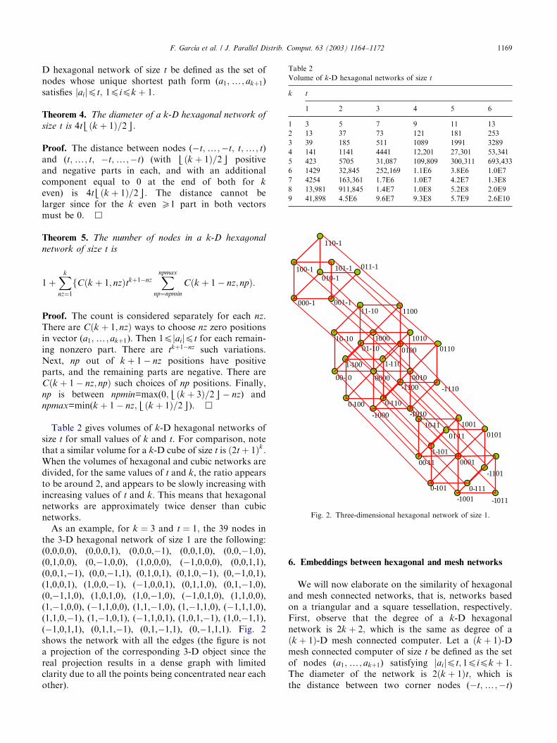
Fig. 2. Three-dimensional hexagonal network of size 1.

There are Cðk þ 1; nzÞ ways to choose nz zero positionsin vector (a1;y; akþ1). Then 1pjaijpt for each remain-ing nonzero part. There are tkþ1�nz such variations.Next, np out of k þ 1� nz positions have positiveparts, and the remaining parts are negative. There areCðk þ 1� nz; npÞ such choices of np positions. Finally,np is between npmin=max(0;Iðk þ 3Þ=2m� nz) andnpmax=min(k þ 1� nz;Iðk þ 1Þ=2m). &

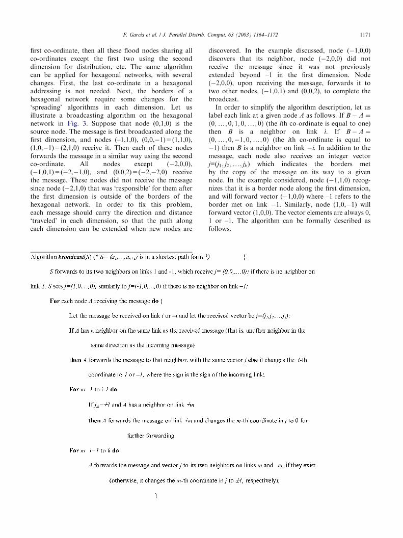
Table 2 gives volumes of k-D hexagonal networks ofsize t for small values of k and t. For comparison, notethat a similar volume for a k-D cube of size t is ð2t þ 1Þk:When the volumes of hexagonal and cubic networks aredivided, for the same values of t and k, the ratio appearsto be around 2, and appears to be slowly increasing withincreasing values of t and k. This means that hexagonalnetworks are approximately twice denser than cubicnetworks.As an example, for k ¼ 3 and t ¼ 1; the 39 nodes in

the 3-D hexagonal network of size 1 are the following:(0,0,0,0), (0,0,0,1), (0,0,0,�1), (0,0,1,0), (0,0,�1,0),(0,1,0,0), (0,�1,0,0), (1,0,0,0), (�1,0,0,0), (0,0,1,1),(0,0,1,�1), (0,0,�1,1), (0,1,0,1), (0,1,0,�1), (0,�1,0,1),(1,0,0,1), (1,0,0,�1), (�1,0,0,1), (0,1,1,0), (0,1,�1,0),(0,�1,1,0), (1,0,1,0), (1,0,�1,0), (�1,0,1,0), (1,1,0,0),(1,�1,0,0), (�1,1,0,0), (1,1,�1,0), (1,�1,1,0), (�1,1,1,0),(1,1,0,�1), (1,�1,0,1), (�1,1,0,1), (1,0,1,�1), (1,0,�1,1),(�1,0,1,1), (0,1,1,�1), (0,1,�1,1), (0,�1,1,1). Fig. 2shows the network with all the edges (the figure is nota projection of the corresponding 3-D object since thereal projection results in a dense graph with limitedclarity due to all the points being concentrated near eachother).

6. Embeddings between hexagonal and mesh networks

We will now elaborate on the similarity of hexagonaland mesh connected networks, that is, networks basedon a triangular and a square tessellation, respectively.First, observe that the degree of a k-D hexagonalnetwork is 2k þ 2; which is the same as degree of aðk þ 1Þ-D mesh connected computer. Let a ðk þ 1Þ-Dmesh connected computer of size t be defined as the setof nodes (a1;y; akþ1) satisfying jaijpt; 1pipk þ 1:The diameter of the network is 2ðk þ 1Þt; which isthe distance between two corner nodes (�t;y;�t)

ARTICLE IN PRESS

1-10

100

000

00-1

-100

0-10

-101 001

10-1

01-1

0-11

-200

00-2

200

002

020

010

-100

0-10

0-11

01-1

1-10

110 10-1 -10-1

-101

11-1

-110

-1-10

-1-11 1-11

1-1-1

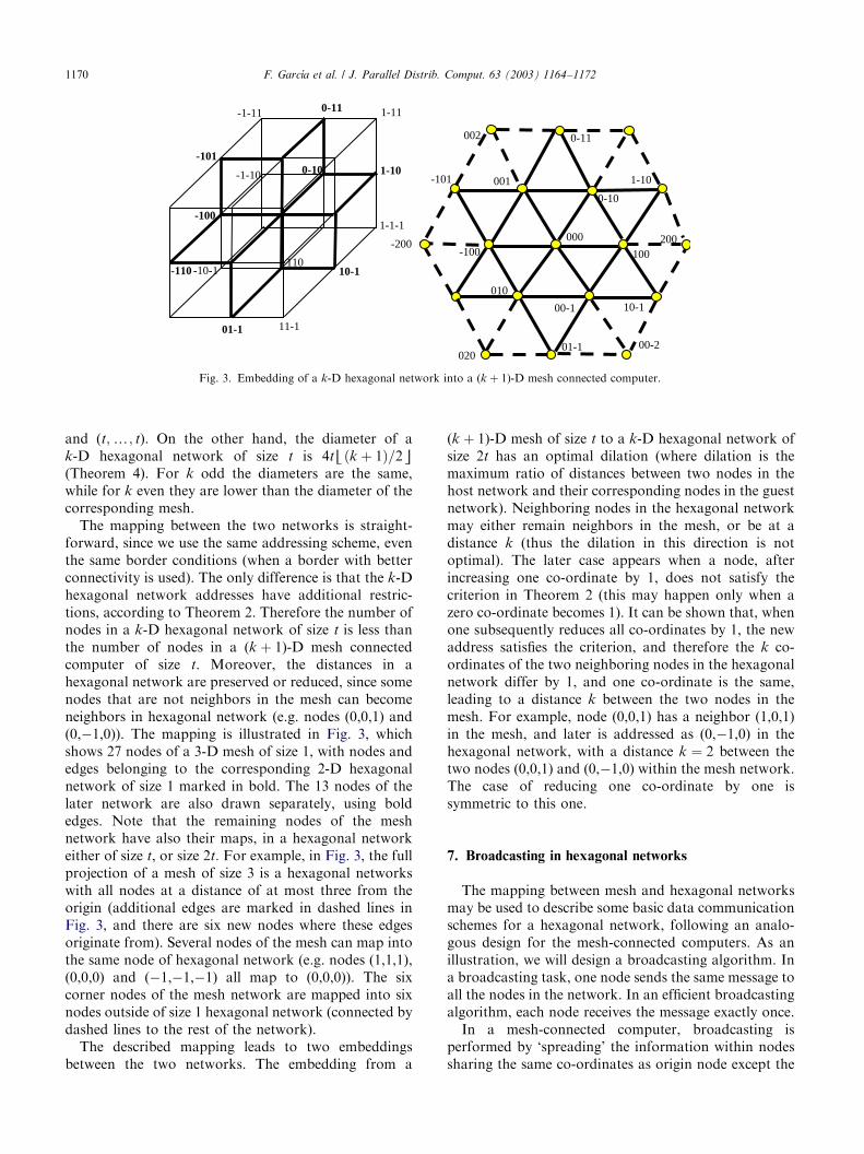
Fig. 3. Embedding of a k-D hexagonal network into a (k þ 1)-D mesh connected computer.

F. Garc!ıa et al. / J. Parallel Distrib. Comput. 63 (2003) 1164–11721170

and (t;y; t). On the other hand, the diameter of ak-D hexagonal network of size t is 4tIðk þ 1Þ=2m(Theorem 4). For k odd the diameters are the same,while for k even they are lower than the diameter of thecorresponding mesh.The mapping between the two networks is straight-

forward, since we use the same addressing scheme, eventhe same border conditions (when a border with betterconnectivity is used). The only difference is that the k-Dhexagonal network addresses have additional restric-tions, according to Theorem 2. Therefore the number ofnodes in a k-D hexagonal network of size t is less thanthe number of nodes in a (k þ 1)-D mesh connectedcomputer of size t. Moreover, the distances in ahexagonal network are preserved or reduced, since somenodes that are not neighbors in the mesh can becomeneighbors in hexagonal network (e.g. nodes (0,0,1) and(0,�1,0)). The mapping is illustrated in Fig. 3, whichshows 27 nodes of a 3-D mesh of size 1, with nodes andedges belonging to the corresponding 2-D hexagonalnetwork of size 1 marked in bold. The 13 nodes of thelater network are also drawn separately, using boldedges. Note that the remaining nodes of the meshnetwork have also their maps, in a hexagonal networkeither of size t, or size 2t: For example, in Fig. 3, the fullprojection of a mesh of size 3 is a hexagonal networkswith all nodes at a distance of at most three from theorigin (additional edges are marked in dashed lines inFig. 3, and there are six new nodes where these edgesoriginate from). Several nodes of the mesh can map intothe same node of hexagonal network (e.g. nodes (1,1,1),(0,0,0) and (�1,�1,�1) all map to (0,0,0)). The sixcorner nodes of the mesh network are mapped into sixnodes outside of size 1 hexagonal network (connected bydashed lines to the rest of the network).The described mapping leads to two embeddings

between the two networks. The embedding from a

(k þ 1)-D mesh of size t to a k-D hexagonal network ofsize 2t has an optimal dilation (where dilation is themaximum ratio of distances between two nodes in thehost network and their corresponding nodes in the guestnetwork). Neighboring nodes in the hexagonal networkmay either remain neighbors in the mesh, or be at adistance k (thus the dilation in this direction is notoptimal). The later case appears when a node, afterincreasing one co-ordinate by 1, does not satisfy thecriterion in Theorem 2 (this may happen only when azero co-ordinate becomes 1). It can be shown that, whenone subsequently reduces all co-ordinates by 1, the newaddress satisfies the criterion, and therefore the k co-ordinates of the two neighboring nodes in the hexagonalnetwork differ by 1, and one co-ordinate is the same,leading to a distance k between the two nodes in themesh. For example, node (0,0,1) has a neighbor (1,0,1)in the mesh, and later is addressed as (0,�1,0) in thehexagonal network, with a distance k ¼ 2 between thetwo nodes (0,0,1) and (0,�1,0) within the mesh network.The case of reducing one co-ordinate by one issymmetric to this one.

7. Broadcasting in hexagonal networks

The mapping between mesh and hexagonal networksmay be used to describe some basic data communicationschemes for a hexagonal network, following an analo-gous design for the mesh-connected computers. As anillustration, we will design a broadcasting algorithm. Ina broadcasting task, one node sends the same message toall the nodes in the network. In an efficient broadcastingalgorithm, each node receives the message exactly once.In a mesh-connected computer, broadcasting is

performed by ‘spreading’ the information within nodessharing the same co-ordinates as origin node except the

ARTICLE IN PRESSF. Garc!ıa et al. / J. Parallel Distrib. Comput. 63 (2003) 1164–1172 1171

first co-ordinate, then all these flood nodes sharing allco-ordinates except the first two using the seconddimension for distribution, etc. The same algorithmcan be applied for hexagonal networks, with severalchanges. First, the last co-ordinate in a hexagonaladdressing is not needed. Next, the borders of ahexagonal network require some changes for the‘spreading’ algorithms in each dimension. Let usillustrate a broadcasting algorithm on the hexagonalnetwork in Fig. 3. Suppose that node (0,1,0) is thesource node. The message is first broadcasted along thefirst dimension, and nodes (–1,1,0), (0,0,�1)=(1,1,0),(1,0,�1)=(2,1,0) receive it. Then each of these nodesforwards the message in a similar way using the secondco-ordinate. All nodes except (�2,0,0),(�1,0,1)=(�2,�1,0), and (0,0,2)=(�2,�2,0) receivethe message. These nodes did not receive the messagesince node (�2,1,0) that was ‘responsible’ for them afterthe first dimension is outside of the borders of thehexagonal network. In order to fix this problem,each message should carry the direction and distance‘traveled’ in each dimension, so that the path alongeach dimension can be extended when new nodes are

discovered. In the example discussed, node (�1,0,0)discovers that its neighbor, node (�2,0,0) did notreceive the message since it was not previouslyextended beyond –1 in the first dimension. Node(�2,0,0), upon receiving the message, forwards it totwo other nodes, (�1,0,1) and (0,0,2), to complete thebroadcast.In order to simplify the algorithm description, let us

label each link at a given node A as follows. If B � A ¼ð0;y; 0; 1; 0;y; 0Þ (the ith co-ordinate is equal to one)then B is a neighbor on link i. If B � A ¼ð0;y; 0;�1; 0;y; 0Þ (the ith co-ordinate is equal to�1) then B is a neighbor on link �i. In addition to themessage, each node also receives an integer vectorj=(j1; j2;y; jk) which indicates the borders metby the copy of the message on its way to a givennode. In the example considered, node (�1,1,0) recog-nizes that it is a border node along the first dimension,and will forward vector (�1,0,0) where –1 refers to theborder met on link �1. Similarly, node (1,0,�1) willforward vector (1,0,0). The vector elements are always 0,1 or –1. The algorithm can be formally described asfollows.

ARTICLE IN PRESSF. Garc!ıa et al. / J. Parallel Distrib. Comput. 63 (2003) 1164–11721172

8. Conclusion

It is an interesting open problem to extend ouraddressing and routing schemes and define a higherdimensional hexagonal tori as an alternative to thepopular t-ary k-cubes. A similar open problem is todefine a higher dimensional honeycomb tori, extendingthe work done in [7].There are a number of topological properties and data

communication algorithms that need to be investigatedfor the proposed network before a final conclusion canbe made. This paper certainly provides a promisingstarting point. In particular, the prefix computation, theHamiltonian path and the disjoint path problems, theembeddings with other networks, the bisection width andthe fault tolerance, among others. Given some borderconditions, it is also interesting to design formulas forranking and unranking the nodes, that is matching theintroduced addresses with the addresses 1; 2;y; n; wheren is the number of nodes in the network.

Acknowledgments

This research is supported by CONACYT Project37017-A and NSERC grants.

References

[1] E. Anderson, J. Brooks, C. Grass, S. Scott, Performance of the

Cray T3E multiprocessor, Proceedings of the Supercomputing

Conference, 1997.

[2] M.M. Bae, B. Bose, Resource placement in torus-based networks,

IEEE Trans. Comput. 46 (10) (1997) 1083–1092.

[3] B. Bose, B. Broeg, Y. Kwon, A. Ashir, Lee distance and

topological properties of k-ary n-cubes, IEEE Trans. Comput.

44 (1995) 1021–1030.

[4] J. Carle, Etude des proprietes des reseaux d’interconnexion de

type nid d’abeilles, Ph.D.Thesis, Laboratoire de Recherche en

Informatique d’Amiens LARIA, Universite de Picardie, Jules

Verne, Amiens, France, December 2000.

[5] J. Carle, J.F. Myoupo, Topological properties and optimal

routing algorithms for three dimensional hexagonal networks,

Proceedings of the High Performance Computing in the

Asia-Pacific Region HPC-Asia, Vol. I, Beijing, China, 2000,

pp. 116–121.

[6] J. Carle, J.F. Myoupo, D. Seme, All-to-all broadcasting

algorithms on honeycomb networks and applications, Parallel

Process. Lett. 9 (4) (1999) 539–550.

[7] J. Carle, J.F. Myoupo, I. Stojmenovic, Higher dimensional

honeycomb networks, J. Interconnect. Networks 2(4) (December

2001) 391–420.

[8] M.S. Chen, K.G. Shin, D.D. Kandlur, Addressing, routing and

broadcasting in hexagonal mesh multiprocessors, IEEE Trans.

Comput. 39 (1) (1990) 10–18.

[9] J.W. Dolter, P. Ramanathan, K.G. Shin, Performance

analysis of virtual cut-through switching in HARTS: a hexagonal

mesh multicomputer, IEEE Trans. Comput. 40 (6) (1991)

669–680.

[10] J. Duato, S. Yalamanchili, L. Ni, Interconnection Networks: An

Engineering Approach, IEEE Computer Society Press, Silver

Spring, MD, 1997.

[11] F. Garcıa, I. Stojmenovic, J. Zhang, Addressing and

routing in hexagonal networks with applications for

location update and connection rerouting in cellular networks,

IEEE Trans. Parallel Distrib. Systems 13(9) (September 2002)

963–971.

[12] R.E. Kessler, J.L. Schwarzmeier, Cray T3D: A new dimension for

Cray Research, in: CompCon, Spring 1993, pp. 176–182.

[13] L.N. Laster, J. Sandor, Computer graphics on hexagonal grid,

Comput. Graph. 8 (1984) 401–409.

[14] G.M. Megson, X. Liu, X. Yang, Fault-tolerant ring embedding in

a honeycomb torus with node failures, Parallel Process. Lett. 9 (4)

(1999) 551–562.

[15] G.M. Megson, X. Yang, X. Liu, Honeycomb tori are Hamilto-

nian, Inform. Process. Lett. 72 (1999) 99–103.

[16] N-Cube Company, NCUBE-2 Processor Manual, N-Cube

Company, 1990.

[17] M. Noakes, W.J. Dally, System design of the J-machine,

Proceedings of the Advanced Research in VLSI, MIT Press,

Cambridge, MA, 1990, pp. 179–192.

[18] B. Parhami, D.-M. Kwai, A unified formulation of honeycomb

and diamond networks, IEEE Trans. Parallel Distrib. Systems

12(1) (January 2001) 74–79.

[19] C. Peterson, et al., iWarp: a 100-MOPS VLIW microprocessor for

multicomputers, IEEE Micro 11 (2) (1991) 26–37.

[20] B. Robic, J. Silc, High performance computing on a honeycomb

architecture, Proceeedings of the International ACPC Parallel

Computation Conference, Lecture Notes in Computer Science,

Austria, 1993.

[21] K.G. Shin, HARTS: a distributed real-time architecture, IEEE

Comput. 24 (5) (1991) 25–35.

[22] I. Stojmenovic, Honeycomb networks: topological properties and

communication algorithms, IEEE Trans. Parallel Distrib. Systems

8(10) (October 1997) 1036–1042.

[23] I. Stojmenovic, Direct interconnection networks, in: A.Y.

Zomaya (Ed.), Parallel and Distributed Computing Handbook,

McGraw-Hill, Inc., Tokyo, 1996, pp. 537–567.

[24] R. Tosic, D. Masulovic, I. Stojmenovic, J. Brunvoll, B.N. Cyvin,

S.J. Cyvin, Enumeration of polyhex hydrocarbons up to h=17, J.

Chem. Inform. Comput. Sci. 35 (1995) 181–187.

[25] J. Zhang, A cell ID assignment scheme and its applications,

Proceedings of the Workshop on Wireless Networks and Mobile

Computing, IEEE International Conference on Parallel Proces-

sing, Toronto, Canada, August 2000, pp. 507–512.