higher-order delta processing for dynamic, frequently fresh views

DBToaster: Higher-order Delta Processing for

Dynamic, Frequently Fresh Views∗

Yanif Ahmad Oliver Kennedy, Christoph Koch, and Milos [email protected] {christoph.koch, oliver.kennedy, milos.nikolic}@epfl.ch

Johns Hopkins University Ecole Polytechnique Federale de Lausanne

ABSTRACTApplications ranging from algorithmic trading to scientificdata analysis require realtime analytics based on views overdatabases that change at very high rates. Such views haveto be kept fresh at low maintenance cost and latencies. Atthe same time, these views have to support classical SQL,rather than window semantics, to enable applications thatcombine current with aged or historical data.

In this paper, we present viewlet transforms, a recursivefinite differencing technique applied to queries. The viewlettransform materializes a query and a set of its higher-orderdeltas as views. These views support each other’s incremen-tal maintenance, leading to a reduced overall view mainte-nance cost. The viewlet transform of a query admits efficientevaluation, the elimination of certain expensive query oper-ations, and aggressive parallelization. We develop viewlettransforms into a workable query execution technique, presenta heuristic and cost-based optimization framework, and re-port on experiments with a prototype dynamic data man-agement system that combines viewlet transforms with anoptimizing compilation technique. The system supports tensof thousands of complete view refreshes a second for a widerange of queries.

1. INTRODUCTIONData analytics has been dominated by after-the-fact ex-

ploration in classical data warehouses for multiple decades.This is now beginning to change: Today, businesses, engi-neers and scientists are increasingly placing data analyticsengines earlier in their workflows to react to signals in freshdata. These dynamic datasets exhibit a wide range of up-date rates, volumes, anomalies and trends. Responsive an-alytics is an essential component of computing in finance,telecommunications, intelligence, and critical infrastructuremanagement, and is gaining adoption in operations, logis-tics, scientific computing, and web and social media analysis.

Developing suitable analytics engines remains challenging.The combination of frequent updates, long-running queriesand a large stateful working set precludes the exclusive use

∗This work was supported by ERC Grant 279804.

of OLAP, OLTP, or stream processors. Furthermore queryrequirements on updates often do not fall singularly intothe functionality and semantics provided by the availabletechnologies, from CEP engines to triggers, active databases,and database views.

Our work on dynamic data management systems (DDMS)in the DBToaster project [3, 19, 18] studies the foundations,algorithms and architectures of data management tools de-signed for large datasets that evolve rapidly through high-rate update streams. A DDMS focuses on long-runningqueries as the norm, alongside sporadic exploratory query-ing. A guiding design principle for DDMS is to take fulladvantage of incremental processing techniques that max-imally reuse prior work. Incremental computation is cen-tral to both stream processing to minimize work as windowsslide, and to database views with incremental view mainte-nance (IVM). DDMS aim to combine some of the advantagesof DBMS (expressive queries over both recent and histori-cal data, without the restrictions of window semantics) andCEP engines (low latency and high view refresh rates).

An example use case is algorithmic trading. Here, strategydesigners want to use analytics expressible in a declarativelanguage like SQL on order book data in their algorithms.Order books consist of the orders waiting to be executed at astock exchange and change very frequently. However, someorders may stay in the order book relatively long before theyare executed or revoked, precluding the use of stream engineswith window semantics. Applications such as scientific sim-ulations and intelligence analysis also exhibit entities whichcapture our attention for widely ranging periods of time,resulting in large stateful and dynamic computation.

The technical focus of this paper is on an extreme formof incremental view maintenance that we call higher-orderIVM. We make use of discrete forward differences (deltaqueries) recursively, on multiple levels of derivation. Thatis, we use delta queries (“first-order deltas”) to incremen-tally maintain the view of the input query, then materializethe delta queries as views too, maintain these views usingdelta queries to the delta queries (“second-order deltas”),and continue alternating between materializing views andderiving higher-order delta queries for maintenance. Thetechnique’s use of higher-order deltas is quite different fromearlier work on trading off choices in which query subex-pressions to materialize and incrementally maintain for bestperformance [27]. Instead, our technique for constructinghigher-order delta views is somewhat reminiscent of discretewavelets and numerical differentiation methods, and we usea superficial analogy to the Haar wavelet transform as mo-tivation for calling the base technique a viewlet transform.

Example 1 Consider a query Q that counts the numberof tuples in the product of relations R and S. For now,we only want to maintain the view of Q under insertions.

Denote by ∆R (resp. ∆S) the change to a view as one tupleis inserted into R (resp., S). Suppose we simultaneouslymaterialize the four views

• Q (0-th order),

• ∆RQ = count(S) and ∆SQ = count(R) (first order), and

• ∆R(∆SQ) = ∆S(∆RQ) = 1 (second order, a “delta of adelta query”).

Then we can simultaneously maintain all these views usingeach other, using exclusively summation and avoiding thecomputation of any products. The fourth view is constantand does not depend on the database. Each of the otherviews is refreshed when a tuple is inserted by adding theappropriate delta view. For instance, as a tuple is insertedinto R, we add ∆RQ to Q and ∆R∆SQ to ∆SQ. (No changeis required to ∆RQ, since ∆R∆RQ = 0.) Suppose R con-tains 2 tuples and S contains 3 tuples. If we add a tuple toS, we increment Q by 2 (∆SQ) to obtain 8 and ∆RQ by 1(∆S∆RQ) to get 4. If we subsequently insert a tuple intoR, we increment Q by 4 (∆RQ) to 12 and ∆SQ by 1 to 3.Two further inserts of S tuples yield the following sequenceof states of the materialized views:

time insert ∆R∆SQ,point into ||R|| ||S|| Q ∆RQ ∆SQ ∆S∆RQ

0 – 2 3 6 3 2 11 S 2 4 8 4 2 12 R 3 4 12 4 3 13 S 3 5 15 5 3 14 S 3 6 18 6 3 1

Again, the main benefit of using the auxiliary views is thatwe can avoid computing the product R × S (or in general,joins) by simply summing up views. In this example, theview values of the (k + 1)-th row can be computed by justthree pairwise additions of values from the k-th row. ✷

This is the simplest possible example query for which theviewlet transform includes a second-order delta query, omit-ting any complex query features (e.g., predicates, self-joins,nested queries). Viewlet transforms can handle general up-date workloads including deletions and updates, as well asqueries with multi-row results.

For a large fragment of SQL, higher-order IVM avoidsjoin processing in any form, reducing all the view refresh-ment work to summation. Indeed, joins are only neededin the presence of inequality joins and nested aggregates inview definitions. The viewlet transform performs repeated(recursive) delta rewrites. Nested aggregates aside, each k-th order delta is structurally simpler than the (k − 1)-thorder delta query. The viewlet transform terminates, as forsome n, the n-th order delta is guaranteed to be constant,only depending on the update but not on the database. Inthe above example, the second-order delta is constant, notusing any database relation.

Our higher-order IVM framework, DBToaster, realizes as-incremental-as-possible query evaluation over SQL with aquery language extending the bag relational algebra, querycompilation and a variety of novel materialization and opti-mization strategies. DBToaster bears the promise of provid-ing materialized views of complex long-running SQL queries,without window semantics or other restrictions, at very highview refresh rates. The data may change rapidly, and stillpart of it may be long-lived. A DDMS can use this func-tionality as the basis for richer query constructs than thosesupported by stream engines. DBToaster takes as inputSQL view queries, and automatically incrementalizes theminto procedural C++ trigger code where all work reduces tofine-grained, low-cost updates of materialized views.

Example 2 Consider the query

Q = select sum(LI.PRICE * O.XCH)from Orders O, LineItem LI where O.ORDK = LI.ORDK;

on a TPC-H like schema of Orders and Lineitem in whichlineitems have prices and orders have currency exchangerates. The query asks for total sales across all orders weightedby exchange rates. We materialize the views for query Q aswell as the first-order views Q LI (∆LIQ) and Q O (∆OQ).The second-order deltas are constant w.r.t. the database andhave been inlined in the following insert trigger programsthat our approach produces for query Q.

on insert into O values (ordk, custk, xch) do {Q += xch * Q_O[ordk];Q_LI[ordk] += xch;

}on insert into LI values (ordk, partk, price) do {

Q += price * Q_LI[ordk];Q_O[ordk] += price;

}

The query result is again scalar, but the auxiliary views arenot, and our language generalizes them from SQL’s multi-sets to maps that associate multiplicities with tuples. Thisis again a very simple example (more involved ones are pre-sented throughout the paper), but it illustrates somethingnotable: while classical incremental view maintenance has toevaluate the first-order deltas, which takes linear time (e.g.,(∆OQ)[ordk] is select sum(LI.PRICE) from Lineitem LIwhere LI.ORDK=ordk), we get around this by performingIVM of the deltas. This way our triggers can be evaluatedin constant time for single-tuple inserts in this example.

The delete triggers for Q are the same as the insert triggerswith += replaced by -= everywhere. ✷

This example presents single-tuple update triggers. View-let transforms are not limited to this but support bulk up-dates. However, delta queries for single-tuple updates haveconsiderable additional optimization potential, which ourcompiler leverages to create very efficient code that refreshesviews whenever a new update arrives. We do not queue up-dates for bulk processing, and so maximize view availabilityand minimize view refresh latency, enabling ultra-low la-tency monitoring and algorithmic trading applications.

On paper, higher-order IVM clearly dominates classicalIVM. If classical IVM is a good idea, then doing it recur-sively is an even better idea. The same efficiency improve-ment argument in favor of IVM of the base query also holdsfor IVM of the delta query. Considering that joins are expen-sive and this approach eliminates them, higher-order IVMhas the potential for excellent query performance.

In practice, how well do our expectations of higher-orderIVM translate into real performance gains? A priori, thecosts associated with storing and managing additional auxil-iary materialized views for higher-order delta queries mightbe more considerable than expected. This paper presentsthe lessons learned in an effort to realize higher-order IVM,and to understand its strengths and drawbacks. Our contri-butions are as follows:

1. We present the concept of higher-order IVM and describethe viewlet transform. This part of the paper generalizesand consolidates our earlier work [3, 19].

2. There are cases (inequality joins and certain nesting pat-terns) when a naive viewlet transform is too aggressive,and certain parts of queries are better re-evaluated thanincrementally maintained. We develop heuristics and acost-based optimization framework for trading off mate-rialization and lazy evaluation for best performance.

3. We have built the DBToaster system which implementshigher-order IVM. It combines an optimizing compilerthat creates efficient update triggers based on the tech-niques discussed above, and a runtime system (currentlysingle-core and main-memory based1) to keep views con-tinuously fresh as updates stream in at high data rates.

4. We present the first set of extensive experimental re-sults on higher-order IVM obtained using DBToaster.Our experiments indicate that frequently, particularlyfor queries that consist of many joins or nested aggrega-tion subqueries, our compilation approach dominates thestate of the art, often by multiple orders of magnitude.On a workload of automated trading and ETL queries,we show that current systems cannot sustain fresh viewsat the rates required in algorithmic trading and real-timeanalytics, while higher-order IVM takes a significant stepto making these applications viable.

Most of our benchmark queries contain features such asnested subqueries that no commercial IVM implementationsupports, while our approach handles them all.

2. RELATED WORK2.1 A Brief Survey of IVM Techniques

Database view management is a well-studied area withover three decades of supporting literature. We focus on theaspects of view materialization most pertinent to DDMS.

Incremental Maintenance Algorithms, and FormalSemantics. Maintaining query answers has been consid-ered under both the set [6, 7] and bag [8, 14] relational alge-bra. Generally, given a query on N relations Q(R1, . . . , RN ),classical IVM uses a first-order delta query ∆R1Q = Q(R1∪∆R1, R2, . . . RN ) − Q(R1, . . . , RN ) for each input relationRi in turn. The creation of delta queries has been studiedfor query languages with aggregation [25] and bag seman-tics [14], but we know of no work that investigates deltaqueries of nested and correlated subqueries. [17] has con-sidered view maintenance in the nested relational algebra(NRA), however this has not been widely adopted in anycommercial DBMS. Finally, [33] considered temporal views,and [22] outer joins and nulls, all for flat SPJAG querieswithout generalizing to subqueries, the full compositional-ity of SQL, or the range of standard aggregates.

Materialization and Query Optimization Strategies.Selecting queries to materialize and reuse during processinghas spanned fine-grained approaches from subqueries [27]and partial materialization [20, 28], to coarse-grained meth-ods as part of multiquery optimization and common subex-pressions [16, 35]. Picking views from a workload of queriestypically uses the AND-OR graph representations from mul-tiquery optimization [16, 27], or adopts signature and sub-sumption methods for common subexpressions [35]. [27]picks additional views to materialize amongst subqueries ofthe view definition, but only performs first-order mainte-nance and does not consider the full framework (bindingpatterns, etc) required with higher-order deltas. Further-more, the optimal set of views is chosen based on the main-tenance costs alone, from a search space that can be doublyexponential in the number of query relations.

Physical DB designers [2, 36] often use the query opti-mizer as a subcomponent to manage the search space ofequivalent views, reusing its rewriting and pruning mecha-nisms. For partial materialization methods, ViewCache [28]1This is not an intrinsic limitation of our method, in fact ourtrigger programs are particularly nicely parallelizable [19].

and DynaMat [20] use materialized view fragments, the for-mer materializing join results by storing pointers back toinput tuples, the latter subject to a caching policy based onrefresh time and cache space overhead constraints.

Evaluation Strategies. To realize efficient maintenancewith first-order delta queries, [9, 34] studied eager and lazyevaluation to balance query and update workloads, and asbackground asynchronous processes [29], to achieve a vari-ety of view freshness models and constraints [10]. Evaluat-ing maintenance queries has also been studied extensivelyin Datalog with semi-naive evaluation (which also uses first-order deltas) and DRed (delete-rederive) [15]. Finally, [13]argues for view maintenance in stream processing, whichreinforces our position of IVM as a general-purpose changepropagation mechanism for collections, on top of which win-dow and pattern constructs can be defined.

2.2 Update Processing MechanismsTriggers and Active Databases. Triggers, active databaseand event-condition-action (ECA) mechanisms [4] providegeneral purpose reactive behavior in a DBMS. The litera-ture considers recursive and cascading trigger firings, andrestrictions to ensure restricted propagation. Trigger-basedapproaches require developers to manually convert queriesto delta form, a painful and error-prone process especiallyin the higher-order setting. Without manual incremental-ization, triggers suffer from poor performance and cannotbe optimized by a DBMS when written in C or Java.

Data Stream Processing. Data stream processing [1, 24]and streaming algorithms combine two aspects of handlingupdates: i) shared, incremental processing (e.g. sliding win-dows, paired vs paned windows), ii) sublinear algorithms(i.e. polylogarithmic space bounds). The latter are approx-imate processing techniques that are difficult to programand compose, and have had limited adoption in commercialDBMS. Advanced processing techniques in the streamingcommunity also focus almost entirely on approximate tech-niques when processing cannot keep up with stream rates(e.g. load shedding, prioritization [30]), on shared process-ing (e.g. on-the-fly aggregation [21]), or specialized algo-rithms and data structures [11]. Our approach to stream-ing is about generalizing incremental processing to (non-windowed) SQL semantics (including nested subqueries andaggregates). Of course, windows can be expressed in thissemantics if desired. Similar principles are discussed in [13].Automatic Differentiation and Incrementalization,and Applications. Beyond the database literature, theprogramming language literature has studied automatic in-crementalization [23], and automatic differentiation. Au-tomatic incrementalization is by no means a solved chal-lenge, especially when considering general recursion and un-bounded iteration. Automatic differentiation considers deltasof functions applied over scalars rather than sets or collec-tions, and lately in higher-order fashion [26]. Bridging thesetwo areas of research would be fruitful for DDMS to supportUDFs and general computation on scalars and collections.

3. QUERIES AND DELTASIn this section, we fix a formalism for queries that makes

it easy to talk cleanly and concisely about delta processing,and we describe the construction of delta queries.

3.1 Data Model and Query LanguageOur data model generalizes multiset relations (as in SQL)

to tuple multiplicities that are rational numbers. This forone allows us to treat databases and updates uniformly (for

R �A, B� #�a, b1� �→ 2�a, b2� �→ −3

S1 �B, C� #�b1, c1� �→ 2�b1, c2� �→ −10

S2 �B, C� #�b1, c1� �→ 3�b1, c2� �→ 3�b2, c1� �→ −11

S1 + S2 �B, C� #�b1, c1� �→ 5�b1, c2� �→ −7�b2, c1� �→ −11

R �� (S1 + S2) �A, B, C� #�a, b1, c1� �→ 10�a, b1, c2� �→ −14�a, b2, c1� �→ 33

SumAC;1/2(R �� (S1 + S2)) �A, C� #�a, c1� �→ 21.5�a, c2� �→ −7

Figure 1: Examples of union, join, and aggregationof generalized multiset relations with rational num-ber tuple multiplicities.

instance, a delete is a relation with negative multiplicities,and applying it to a database means unioning/adding it tothe database). It also allows us to use multiplicities to rep-resent aggregate query results (which do not need to be inte-gers). As a consequence, when performing delta-processingon aggregate queries, growing an aggregate means addingto the aggregate value rather than to delete the tuple withthe old aggregate value and insert a tuple with the new ag-gregate value. Maintaining aggregates in the multiplicitiesallows for simpler and cleaner bookkeeping. It is a cosmeticchange that does not keep us from supporting SQL queries.

Formally, a thus generalized multiset relation (GMR) is afunction from tuples to rational numbers, with finite support(i.e., only a finite number of tuples have nonzero multiplic-ity). The union, join, selection, and grouping-sum-aggregateoperations are defined in the way that naturally generalizesthe same operations on multiset relations:

R + S : �t �→ R(�t) + S(�t)

R �� S : �t �→

8<

:

R(πsch(R)�t) ∗ S(πsch(S)�t). . . �t = πsch(R)∪sch(S)(�t)

0 . . . otherwise

σθR : �t �→

R(�t) . . . θ(�t) is true0 . . . otherwise

Sum �A;fR : �a �→X

π �A(�t)=�a

R(�t) ∗ f(�t)

Here, π is the projection of records, rather than relations,removing fields of �t whose labels are not among the columnnames �A, and sch(R) denotes the list of column names ofGMR R. An aggregation Sum �A;fR almost works like the

SQL query select �A, sum(f) from R group by �A, withthe difference that SQL puts the aggregate value into a newcolumn, while Sum �A;fR puts it into the multiplicity of thegroup-by tuple. Aggregations can also serve as multiplicity-preserving projections, and a query Sum �A;1(R) corresponds

equivalently to SQL queries select �A from R and select�A, sum(1) from R group by �A. Examples of join, union,and aggregation are shown in Figure 1.

Our query language includes relational atoms R, constantsingleton relations, natural join, union (denoted +), selec-tion, grouping sum-aggregates, and column renaming ρ:

Q ::= R | { �A : �a �→ c} |Q �� Q |Q + Q |σφQ | Sum �A;fQ | ρ �AQ

where the c are rational numbers, f are terms, and φ areconditions over terms. Terms are define using arithmeticsover rational constants and column names. Additionallywe can use non-grouping aggregates as terms (the value is

the multiplicity), specifically in selection conditions. Thatway we can express queries with nested aggregates. Nestedaggregates may be correlated with the outside in the way weare used to from SQL. For example, we write σC<SumA;BRS

for the SQL query

select * from Swhere S.C < (select sum(B) from R where R.A=S.A)

We can perform deletions writing R − S, and this is nofundamentally new operation since we can define R − S :=R + (S �� {�� → −1}). Here {�� → −1} is a nullary case ofsingleton GMR construction { �A : �a �→ c}.

There is no explicit syntax for universal quantification/re-lational difference or aggregates other than Sum, but allthese features can be expressed using (nested) sum-aggregatequeries (a popular homework exercise in database courses).Special handling of these features in delta processing andquery optimization could yield performance better than whatwe report in our experiments. However, granting these de-finable features specialized treatment is beyond the scope ofthis paper. As a consequence, our implementation providesnative support for only the fragment presented above andthe experiment use only techniques described in the paper.

We will use relational algebra and SQL syntax interchange-ably as we are used to from bag relational algebra and SQL.

3.2 Computing the Delta of a QueryWe next show how to construct delta queries. The reader

familiar with incremental view maintenance may skip thissection, but note that the algebra just fixed has the niceproperty of being closed under taking deltas. For each queryexpression Q, there is an expression ∆Q of the same algebrathat expresses how the result of Q changes as the databaseD is changed by update workload ∆D,

∆Q(D, ∆D) := Q(D + ∆D)−Q(D).

Thanks to the strong compositionality of the language,we only have to give delta rules for the individual operators.These rules are given and studied in detail in [19]. In short,

∆(Q1 + Q2) := (∆Q1) + (∆Q2),

∆(Sum �A;f Q) := Sum �A;f (∆Q),

∆(Q1 �� Q2) := ((∆Q1) �� Q2) + (Q1 �� (∆Q2))

+ ((∆Q1) �� (∆Q2)),

∆(σθQ) := σθ(∆Q).

∆R is the update to R. In the case that the update doesnot change R (but other relation(s)), ∆R is empty.

Here we assume that f and θ do not contain nested ag-gregates. Achieving the full generality is not a technicalproblem, but requires notation beyond the scope of thispaper; we refer to [19] for the general case. We will seein Section 5 that, in practice, we will not need deltas forconditions with nested aggregates, as we will decide to re-evaluate rather than materialize and incrementally maintainsuch conditions.

Example 3 Given schema R(AB), S(CD), and query

select sum(A * D) from R, S where B = C

or, in the algebra, Sum��;A∗D(σB=C(R �� S)). Modulo names,this is the query of Example 2. The delta for this query as

we apply a change ∆R to relation R but leave S unchanged(∆S is empty) is

∆Sum��;A∗D(σB=C(R �� S)) =

Sum��;A∗D∆(σB=C(R �� S)) =

Sum��;A∗D(σB=C∆(R �� S))

and by the delta rule for ��,

∆(R �� S) = (∆R) �� S + R �� (∆S) + (∆R) �� (∆S).

Thus the delta query is Sum��;A∗D(σB=C((∆R) �� S)). ✷

The delta rules work for bulk updates. The special caseof single-tuple updates is interesting since it allows us tosimplify delta queries further and to generate particularlyefficient view refresh code.

Example 4 We continue the Example 3, but now assumethat ∆R is an insertion of a single tuple �A : x, B : y�. Thedelta query Sum��;A∗D(σB=C({�A : x, B : y�} �� S)) can besimplified to Sum��;x∗D(σy=CS). ✷

3.3 Binding PatternsQuery expressions have binding patterns: There are in-

put variables or parameters without which we cannot eval-uate these expressions, and there are output variables, thecolumns of the schema of the query result. Each expres-sion Q has input variables or parameters �xin and a set ofoutput variables �xout, which form the schema of the queryresult. We denote such an expression as Q[ �xin][ �xout]. Theinput variables are those that are not range-restricted in acalculus formulation, or equivalently have to be understoodas parameters in an SQL query because their values cannotbe computed from the database: They have to be providedso that the query can be evaluated.

The most interesting case of input variables occurs in acorrelated nested subquery, viewed in isolation. In such asubquery, the correlation variable from the outside is suchan input variable. The subquery can only be computed if avalue for the input variable is given.

Example 5 We illustrate this by an example. Assume re-lation R has columns A, B and relation S has columns C, D.The SQL query

select * from Rwhere B < (select sum(D) from S where A > C)

is equivalent to Sum∗;1(σB<Sum��;D(σA>C(S))R) in the al-gebra. Here, all columns of the schema of R are outputvariables. In the subexpression Sum��;D(σA>C(S)), A is aninput variable; there are no output variables since the ag-gregate is non-grouping. ✷

Also note that taking a delta adds input variables param-eterizing the query with the update. In Example 4 for in-stance, the delta query has input variables x and y to passin the update. Delta queries for bulk updates have relation-valued parameters.

4. THE VIEWLET TRANSFORMWe are now ready for the viewlet transform. If we restrict

the query language to exclude aggregates nested into con-ditions2 (for which the delta query was complicated), thequery language fragment has the following nice property.

2We will eliminate this restriction on the technique in thenext section.

∆Q is structurally strictly simpler than Q when query com-plexity is measured as follows. For union(+)-free queries,the degree deg(Q) of query Q is the number of relationsjoined together. We can use distributivity to push unionsabove joins and so give a degree to queries with unions: themaximum degree of the union-free subqueries. Queries arestrongly analogous to polynomials, and the degree of queriesis defined precisely as it is defined for polynomials (wherethe relation atoms of the query correspond to the variablesof the polynomial).

Theorem 1 ([19]) If deg(Q) > 0, then

deg(∆Q) = deg(Q)− 1.

The viewlet transform makes use of the simple fact thata delta query is a query too. Thus it can be incrementallymaintained, making use of a delta query to the delta query,which again can be materialized and incrementally main-tained, and so on, recursively. By the above theorem, thisrecursive query transformation terminates in the deg(Q)-threcursion level, when the rewritten query is a “constant” in-dependent of the database, and dependent only on updates.

All queries, aggregate or not, map tuples to rational num-bers (= define GMRs). Thus it is natural to think of theviews as map data structures (dictionaries). In this section,we make no notational difference between queries and (ma-terialized) views, but it will be clear from the context thatwe are using views when we increment them.

Definition 1 The viewlet transform turns a query into aset of update triggers that together maintain the view ofthe query and a set of auxiliary views. Assume the queryQ has input variables (parameters) �xin. For each relation R

used in the query, the viewlet transform creates a trigger

on update R values DR do TR.

where DR is the update – a generalized multiset relation –to the relation named R and TR is the trigger body, a set ofstatements. The trigger bodies are most easily defined bytheir computation by a recursive imperative procedure V T

defined below (initially, the statement lists TR are empty):

procedure VT(Q, �xin):foreach relation name R used in Q do {

TR += (foreach �xin do Q[�xin] += ∆RQ[�xinDR])if deg(Q) > 0 then {

let D be a new variable of type relation of schema R;VT(∆RQ, �xinD)

} }

Here, += on TR appends a statement to an imperative codeblock, and += on generalized multiset relations uses the + ofSection 3.1. Exactly those queries occurring in triggers thathave degree greater than zero are materialized. Of course,these are exactly those queries that are added to by triggerstatements: those that are incrementally maintained. ✷

Example 6 For example, if the schema contains two rela-tions R and S and query Q has degree 2, then VT(Q, ��)returns as TR the code block

Q += ∆RQ[DR];foreach D1 do ∆RQ[D1] += ∆R∆RQ[D1, DR];foreach D2 do ∆SQ[D2] += ∆R∆SQ[D2, DR]

The body for the update trigger of S, TS , is analogous. Notethat the order of the first two statements matters. For cor-rectness, we read the old versions of views in a trigger. ✷

The viewlet transform bears a superficial analogy withthe Haar wavelet transform, which also materializes a hi-erarchy of differences; however, these are not differences ofdifferences but differences of recursively computed sums.

At runtime, each trigger statement loops over a relevantsubset of the possible valuations of the parameters of theviews used in the statement. For relation-typed parame-ters, this is a priori astronomically expensive. There arevarious ways of bounding the domains to make this feasible.Furthermore, parameters can frequently be optimized away.Nevertheless, single-tuple updates offer particular optimiza-tion potential, and we focus on these in this paper.

We will study single-tuple insertions, denoted +R(�t) forthe insertion of tuple �t into relation R, and single-tuple dele-tions −R(�t). Here we create insert and delete triggers inwhich the argument is the tuple, rather than a generalizedmultiset relation, and we avoid looping over relation-typedvariables.

Example 7 We return to the query Q of Example 4, withsingle-tuple updates. The query has degree two. The second-order deltas (∆sgnRR(x,y)∆sgnSS(z,u)Q)[x, y, z, u] have valuesgn

Rsgn

SSum��;x∗u(σy=z{��}), which is equivalent to �� →

sgnRsgn

Sif y = z then x ∗ u else 0; here sgn

R, sgn

S∈ {+,−}.

Variables x and y are arguments of the trigger and are boundat runtime, but variables z and u need to be looped over.On the other hand, the right-hand side of the trigger is onlynon-zero in case that y = z. So we can substitute z by y

everywhere and eliminate z. Using this simplification, theon-insert into R trigger +R(x, y) according to the viewlettransform is the program

Q += ∆+R(x,y)Q[x, y];foreach u do ∆+S(y,u)Q[y, u] += {�� → x ∗ u};foreach u do ∆−S(y,u)Q[y, u] -= {�� → x ∗ u}The remaining triggers are constructed analogously. Thetrigger contains an update rule for the (in this case, scalar)view Q for the overall query result, which uses the auxiliaryview ∆±R(x,y)Q which is maintained in the update triggersfor S, plus update rules for the auxiliary views ∆±S(z,u)Q

that are used to update Q in the insertion and deletion trig-gers on updates to S.

The reason why we did not show deltas ∆±R(... )∆±R(... )Q

or ∆±S(... )∆±S(... )Q is that these are guaranteed to be 0,as the query does not have a self-join.

A further optimization, exploiting distributivity and pre-sented in the next section, eliminates the loops on u andleads us to the triggers of Example 2. ✷

We observe that the structure of the work that needs to bedone is extremely regular and (conceptually) simple. More-over, there are no classical large-granularity operators left,so it does not make sense to give this workload to a classicalquery optimizer. There are for-loops over many variables,which have the potential to be very expensive. But thework is also perfectly data-parallel, and there are no datadependencies comparable to those present in joins. All thisprovides justification for making heavy use of compilation.

Note that there are many optimizations not exploited inthe presentation of viewlet transforms. Thus, we will referto the viewlet transform as presented in this section as naiverecursive IVM in the experiments section. We will presentimprovements and optimizations next.

5. OPTIMIZING VIEWLETSIn this section, we present optimizations of the viewlet

transform as well as heuristics and a cost model that allowus to avoid materializing views with high maintenance cost.

Query Decomposition

M(Sum �A �B:f1∗f2(Q1 �� Q2)) ⇒

M(Sum �A:f1(Q1)) �� M(Sum�B:f2

(Q2)) (1)

Q1 and Q2 have no common columns�A and �B are the group-by terms of each

Factorization and Polynomial Expansion

M(QL �� (Q1 + Q2 + . . .) �� QR) ⇔M(QL �� Q1 �� QR) +M(QL �� Q2 �� QR) + . . . (2)

Input Variables

M(Sum �A;f( �B �C)(σθ( �B �C)(Q))) ⇒

Sum �A;f( �B �C)(σθ( �B �C)(M(Sum �A �B;1(Q)))) (3)

f, θ are functions over terms�A is the group-by variables of the aggregate over Q

�B is the output variables of Q used by f, θ

�C is the input variables that do not appear in Q

Nested Aggregates and Decorrelation

M(Sum �A;f (σθ(QN , �B)(QO))) ⇒

Sum �A;1(σθ(M(QN ), �B)(M(Sum �A �B;f (QO)))) (4)

QN is a non-grouping aggregate termf, θ are functions over terms�A is the group-by variables of the aggregate over QO

�B is the output variables of QO used by f, θ and QN

Figure 2: Rewrite rules for partial materialization.

Bidirectional arrows indicate rules that are applied

heuristically or using the cost model from Section 5.1.

5.1 Materialization DecisionsFor any query Q, the naive viewlet transform produces a

single materialized view MQ. However, it is frequently moreefficient to materialize Q piecewise, as a collection of incre-mentally maintained materialized views �MQ and an equiva-lent query Q

� that is evaluated over these materialized views.We refer to the rewritten query and its piecewise maps as amaterialization decision for Q, denoted �Q�

, �MQ�.DBToaster selects a materialization decision for a query

Q iteratively, by starting with the naive materialization de-cision �(MQ,1), (MQ,1 := Q)� and applying several rewriterules up to a fixed point. These rewrite rules are presentedin Figure 2, and are discussed individually below. Figure3 shows the applicability of these rules to the experimentalworkload discussed in Section 6 and Appendix A.

For clarity, we will use a materialization operator M toshow materialization decisions juxtaposed with their corre-sponding queries. For example, one possible materializationdecision for the query Q := Q1 �� Q2 is:

M(Q1) �� M(Q2) ≡ �(MQ,1 �� MQ,2), {MQ,i := Qi}�.

We will first discuss the use of these rules in a heuristicoptimizer, which when applied as aggressively as possibleproduces near-optimal trigger programs for maintaining thevast majority of queries. We also briefly discuss a cost-basedoptimization strategy to further improve performance.Duplicate View Elimination. As the simplest optimiza-tion, we observe that the naive viewlet transform producesmany duplicate views. This is primarily because the deltaoperation typically commutes with itself; ∆R∆SQ = ∆S∆RQ

for any Q that does not contain nested aggregates over R orS. Even simple structural equivalence effectively identifiesthis sort of view duplication. View de-duplication substan-tially reduces the number of views created.

Query Decomposition. DBToaster makes extensive useof the generalized distributive law[5] (which plays an impor-tant role for probabilistic inference with graphical models)to decompose the materialization of expressions with dis-connected join graphs. This rule is presented in Figure 2.1.

If the join graph of Q includes multiple disconnected com-ponents �Qi, Q2, . . . (i.e., Q := Q1 × Q2 × . . .), it is betterto materialize each component independently. The cost ofselecting from, or iterating over Q is identical for both ma-terialization strategies. Furthermore, maintaining each indi-vidual Qi is less computationally expensive; the decomposedmaterialization stores (and maintains) only

Pi|Qi| values,

while the combined materialization handlesQ

i|Qi| values.

This optimization plays a major role in the efficiency ofDBToaster, and in the justification of compilation. Takinga delta of a query with respect to a single-tuple update re-places a relation in the query by a singleton constant tuple,effectively eliminating one hyperedge from the join graphand creating new disconnected components that can be fur-ther decomposed. Query decomposition is also critical forensuring that the number of maps created for any acyclicquery is polynomial.

Polynomial Expansion and Factorization. As describedabove, query decomposition operates exclusively over con-junctive queries. In order to decompose across unions, weobserve that the union operation can be pushed through ag-gregate sums (i.e, Sum(Q1 + Q2) = Sum(Q1) + Sum(Q2)),and distributed over joins.

Any query expression can be expanded into a flattenedpolynomial representation, which consists of a union of purelyconjunctive queries. Query decomposition is then applied toeach conjunctive query individually. This rewriting rule ispresented in Figure 2.2.

Note that this rewrite rule can also be applied in reverse.A polynomial expression can be factorized into a smaller rep-resentation by identifying common subexpressions (QL andQR in the rewrite rule) and pulling them out of the union.The cost-based optimizer makes extensive use of factoriza-tion to fully explore the space of possible materializationdecisions. The heuristic optimizer does not attempt to fac-torize while making a materialization decision. However,after a materialization decision �MQ, {. . .}� is finalized, thematerialized query MQ itself is simplified by factorization.

Input Variables. Queries with input variables have in-finite domains and cannot be fully materialized. By de-fault, DBToaster’s heuristics ensures that input variablesare avoided, in the query and all its subexpressions.

Input variables are originally introduced into an expres-sion by nested aggregates, and as part of deltas. They ap-pear exclusively in selection and aggregation operators.

The rewrite rule shown in Figure 2.3 ensures that mate-rialized expressions do not have input variables by pullingoperators with input variables out of the materialized ex-pression. If an operator can be partitioned into componentswith output variables only and components with input vari-ables, only the latter are pulled out of the expression.

In addition to this heuristic approach, the cost-based op-timizer explores alternative materialization decisions wheresome (or all) of the input variables in an expression are keptin the materialized expression. With respect to Figure 2.3,these input variables are treated as elements of �A instead of�C. At runtime, only a finite portion of the domain of theseinput variables is maintained in the materialized view.

A materialized view with input variables acts, in effect, asa cache for the query results. Unlike a traditional cache how-ever, the contents of this map are not invalidated when theunderlying data changes, but instead maintained incremen-

tally. These sorts of view caches are analogous to partiallymaterialized views [20, 28].

View caches are only beneficial when the size of the activedomain of an input variable is small, and so the heuristicoptimizer does not attempt to create them3.

Deltas of Nested Aggregates. Thus far, we have ignoredqueries containing nested subqueries. When the delta of thenested subquery is nonzero, the delta of the entire query isnot simpler than the original. The full delta rule for nestedpresented in [19] effectively computes the nested aggregatetwice: once to obtain the original value, and once to obtainthe value after incorporating the delta.

Example 8 Consider the following query, with relations R

and S with columns A and B respectively:

Q := Sum��;1(σSum��;1(S)=A(R))

By the delta rule for nested aggregates,

∆+S(B�) := Sum��;1(σSum��;1(S)+1)=A(R))−Sum��;1(σSum��;1(S)=A(R))

Because the original nested query appears in the deltaexpression, the naive viewlet transform will not terminatehere. To address this, the delta query is is decorrelated intoseparate materialized expressions for the nested subqueryand the outer query. The rewrite rule of Figure 2.4 is appliedtwice (once to each instance). Each materialized expressionnow has a lower degree than the original query.

Although this rule is necessary for termination, it intro-duces a computation cost when evaluating the delta query.Note however, that this rule is only required (and thus, onlyused) when the delta of the nested subquery is nonzero.

Example 9 Continuing Example 8, the materialization de-cision for ∆+S(B�)Q uses two materialized views:MQ,1 := Sum��;1(S) and MQ,2 := R, and uses each twice.However, ∆+R(A�)Q naturally has a lower degree than Q,and is thus materialized in its entirety.

Additionally, we observe that for some queries, it is moreefficient to entirely recompute the query Q on certain up-dates. Consider the general form of a nested aggregate:

Q := Sum �A;f1(σ(Sum �A �B;f2

(QO)))

The delta of Q evaluates two nearly identical expressions.Naively, computing the delta costs twice as much as the orig-inal query and so re-evaluation is more efficient. However, ifthe delta’s trigger arguments bind one or more variables in�B, then the delta query only aggregates over a subset of thetuples in QO and will therefore be faster. Based on this anal-ysis, the heuristic optimizer decides whether to re-evaluateor incrementally maintain any given delta query.

Cost Model. While DBToaster’s full cost-based optimizeris beyond the scope of this paper, we now briefly discussits cost model. The dominant processing overheads are: (1)Updating maps with query results, and (2) Sum aggregates,which compound tuples into aggregate values.

The cost of a materialization decision �Q�, �MQ� includes

both an evaluation component (coste) and a maintenancecomponent (costm) for both the view materialized for theoriginal query and all of the higher-order views.3View caching is required for any materialized expressionwithout finite support. This includes some forms of nestedaggregates without input variables. A precise characteriza-tion of these expressions is beyond the scope of this paper.

Rule (1) Rule (2) Rule (3) Rule (4)

Query (S)ubquery (R)e-eval

(C)ache (I)ncremental

Fin

ance

AXF - ✓ S -

BSP - ✓ - -

BSV - ✓ - -

MST - ✓ S R,I

PSP - ✓ S R,I

VWAP - ✓ C R

TPC

H

Q3 ✓ ✓ - -

Q11 - - - -

Q17 ✓ ✓ S I

Q18 ✓ ✓ S I

Q22 ✓ ✓ S R,I

SSB4 ✓ - - -

Figure 3: Rewrite rules applied to our workload.

DBToaster uses standard cardinality estimation [12, 32]for the number of distinct tuples when projecting the resultof query Q down to columns �A. We refer to this as the sizeof the domain of �A in Q (|dom �A

(Q)|). If �A is the full set ofoutput variables of Q, then we refer to this as the completedomain of Q (|dom(Q)|).

Let Q be the set of all subexpressions of Q. The cost ofquery Q is the sum of the sizes of the complete domains ofthe outer query Q and all queries nested immediately insideaggregate sums Qi in Q:

coste(Q) = |dom(Q)| +X

{Qi|Sum(Qi)∈Q}|dom(Qi)|

The maintenance cost of Q is based on the cost of main-taining all the MQ,i ∈ �MQ. Every MQ,i must be updated forevery change to a relation Rj that appears in it. If the deltaquery of MQ,i is materialized using materialization decision�Q�

i,j ,�MQi,j

�, and the rate of insertions into Rj is rateRj,

then the cost of maintaining MQ,i is

costm(MQ,i) =X

Rj

rateRj·coste(Q

�i,j)+

X

M∈ �MQi,j

costm(M)

This definition recurs on the cost of maintaining the mapsrequired to evaluate Qi,j . The maintenance cost of a mapthat is already being materialized by another query is zero.

The full cost of processing query Q is now

cost(Q) = (raterefresh · coste(Q�)) + (

X

i

costm(MQ,i))

where the refresh rate of Q depends on how frequently afresh view must be made available. For the typical usagescenario a refresh occurs on every update, and raterefresh =P

jrateRj

.

5.2 Optimized Viewlet Transform ExampleFigure 4 shows the trigger program compiled from query

Q18 from our test workload (see Appendix A).For simplicity, we use the condensed schema C(CK),

O(CK, OK), and LI(OK, QTY ). The query Q[][CK] is:

SumCK;QTY (

σ100<Sum��;QT Y � (σOK=OK� (ρOK�,QT Y �LI))(C �� O �� LI))

Due to space limitations we only show the derivation of in-sertions into Orders O and Lineitem LI. Insertions intoCustomer C are a simple extension, while deletions are du-als of insertions and are omitted entirely.

Insertions into Orders. The first-order delta of Q forinsertion of a single tuple �CK : ck, OK : ok� is

∆+O�ck,ok�Q := SumCK;QTY (σOK=ok∧CK=ck∧Qns(C �� LI))

where Qns =(100 < Sum��;QTY �(σok=OK�ρOK�,QTY �LI))

on insert into C values (ck) do {01 Q[][ck] += QC [][ck]

02 foreach OK do QLI [][ck, OK] += QLI,C [][ck, OK]

03 QO1[][ck] += 1

}on insert into O values (ck,ok) do {04 Q[][ck] += QO1[][ck] �� QO2[][ok] �� σ100<QO2[][ok](1)

05 QLI [][ck, ok] += QO1[][ck]

06 QLI,C [][ck, ok] += 1

07 QC [][ck] += QO2[][ok] �� σ100<QO2[][ok](1)

}on insert into LI values (ok,qty) do {08 foreach CK do

Q[][CK] += QLI [][CK, ok] �� (

((QO2[][ok] + {�� → qty}) �� σ100<qty+QO2[][ok](1))

− (QO2[][ok] �� σ100<QO2[][ok](1)))

09 foreach CK do

QC [][CK] += QLI,C [][CK, ok] �� (

((QO2[][ok] + {�� → qty}) �� σ100<qty+QO2[][ok](1))

− (QO2[][ok] �� σ100<QO2[][ok](1)))10 QO2[][ok] += qty

}

Figure 4: DBToaster insert trigger program for Q18.

By rewrite rule 1, this delta expression can be decomposedinto two separate maps, since C and LI share no commoncolumns. Furthermore, the nested subexpression does notcontain relation O, so we do not apply rewrite rule 4 here.The delta expression can be materialized as follows:

M(Sum�CK�;1(σCK=ckC)) �� M(Sum��;QTY (

σOK=ok∧(100<Sum��;QT Y � (σok=OK� (ρOK�,QT Y �LI)))LI))

The second materialized map can be simplified further byrules 1 and 4. OK is bound to trigger parameter ok, whichbreaks the join graph between the selection predicate andLI. Then, since the selection predicate is being applied toa singleton, we can safely materialize only the aggregate inthe predicate. Applying these optimizations gives us thefollowing materialization decision (with 1 := {�� → 1}):

M(Sum�CK�;1(σCK=ckC)) ��

M(Sum��;QTY (σOK=okLI)) ��

Sum��;1(σ100<M(Sum��;QT Y (σok=OKLI))(1))

Trigger statement 04 uses the following set of views (notethat QO2 is used twice):

QO1 := SumCK;1(C) QO2 := SumOK;QTY (LI)

QO1[][CK] is maintained on insertions into C with:

∆+C�ck�QO1 := {�CK : ck� �→ 1}which corresponds to trigger statement 03. QO2[][OK] ismaintained similarly with trigger statement 10.

Insertions into Lineitem. The first-order delta of Q forinsertion of a single tuple �OK : ok, QTY : qty� is

∆+LI�ok,qty�Q := SumCK;QTY

`σOK=ok∧100<qty+Qns (

C �� O �� (LI + {�OK : ok, QTY : qty� �→ 1}))− σOK=ok∧100<Qns (C �� O �� LI)

´

When computing the above delta, we extend the delta ruleof [19] for nested aggregates. The delta of a (decorrelated)

0.1

1

10

100

1000

10000

100000

Q3 Q11 Q17 Q18 Q22 SSB4BSV BSP AXF PSP MST

VWAP

Aver

age

Ref

resh

Rat

e (R

elat

ive

To R

epea

ted

Eval

uatio

n)DBXSPY

Depth 0 (Repeated)Depth 1 (IVM)

Naive Recursive*DBToaster

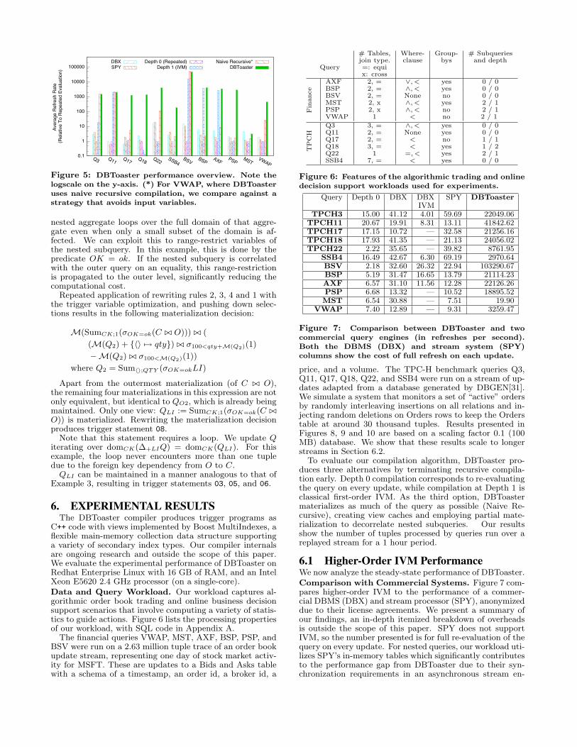
Figure 5: DBToaster performance overview. Note the

logscale on the y-axis. (*) For VWAP, where DBToaster

uses naive recursive compilation, we compare against a

strategy that avoids input variables.

nested aggregate loops over the full domain of that aggre-gate even when only a small subset of the domain is af-fected. We can exploit this to range-restrict variables ofthe nested subquery. In this example, this is done by thepredicate OK = ok. If the nested subquery is correlatedwith the outer query on an equality, this range-restrictionis propagated to the outer level, significantly reducing thecomputational cost.

Repeated application of rewriting rules 2, 3, 4 and 1 withthe trigger variable optimization, and pushing down selec-tions results in the following materialization decision:

M(SumCK;1(σOK=ok(C �� O))) �� (

(M(Q2) + {�� → qty}) �� σ100<qty+M(Q2)(1)

−M(Q2) �� σ100<M(Q2)(1))

where Q2 = Sum��;QTY (σOK=okLI)

Apart from the outermost materialization (of C �� O),the remaining four materializations in this expression are notonly equivalent, but identical to QO2, which is already beingmaintained. Only one view: QLI := SumCK;1(σOK=ok(C ��

O)) is materialized. Rewriting the materialization decisionproduces trigger statement 08.

Note that this statement requires a loop. We update Q

iterating over domCK(∆+LIQ) = domCK(QLI). For thisexample, the loop never encounters more than one tupledue to the foreign key dependency from O to C.

QLI can be maintained in a manner analogous to that ofExample 3, resulting in trigger statements 03, 05, and 06.

6. EXPERIMENTAL RESULTSThe DBToaster compiler produces trigger programs as

C++ code with views implemented by Boost MultiIndexes, aflexible main-memory collection data structure supportinga variety of secondary index types. Our compiler internalsare ongoing research and outside the scope of this paper.We evaluate the experimental performance of DBToaster onRedhat Enterprise Linux with 16 GB of RAM, and an IntelXeon E5620 2.4 GHz processor (on a single-core).Data and Query Workload. Our workload captures al-gorithmic order book trading and online business decisionsupport scenarios that involve computing a variety of statis-tics to guide actions. Figure 6 lists the processing propertiesof our workload, with SQL code in Appendix A.

The financial queries VWAP, MST, AXF, BSP, PSP, andBSV were run on a 2.63 million tuple trace of an order bookupdate stream, representing one day of stock market activ-ity for MSFT. These are updates to a Bids and Asks tablewith a schema of a timestamp, an order id, a broker id, a

# Tables, Where- Group- # Subqueries

join type. clause bys and depth

Query =: equi

x: cross

Fin

ance

AXF 2, = ∨, < yes 0 / 0

BSP 2, = ∧, < yes 0 / 0

BSV 2, = None no 0 / 0

MST 2, x ∧, < yes 2 / 1

PSP 2, x ∧, < no 2 / 1

VWAP 1 < no 2 / 1

TPC

H

Q3 3, = ∧, < yes 0 / 0

Q11 2, = None yes 0 / 0

Q17 2, = < no 1 / 1

Q18 3, = < yes 1 / 2

Q22 1 =, < yes 2 / 1

SSB4 7, = < yes 0 / 0

Figure 6: Features of the algorithmic trading and online

decision support workloads used for experiments.

Query Depth 0 DBX DBX SPY DBToasterIVM

TPCH3 15.00 41.12 4.01 59.69 22049.06TPCH11 20.67 19.91 8.31 13.11 41842.62TPCH17 17.15 10.72 — 32.58 21256.16TPCH18 17.93 41.35 — 21.13 24056.02TPCH22 2.22 35.65 — 39.82 8761.95

SSB4 16.49 42.67 6.30 69.19 2970.64BSV 2.18 32.60 26.32 22.94 103290.67BSP 5.19 31.47 16.65 13.79 21114.23AXF 6.57 31.10 11.56 12.28 22126.26PSP 6.68 13.32 — 10.52 18895.52MST 6.54 30.88 — 7.51 19.90

VWAP 7.40 12.89 — 9.31 3259.47

Figure 7: Comparison between DBToaster and two

commercial query engines (in refreshes per second).

Both the DBMS (DBX) and stream system (SPY)

columns show the cost of full refresh on each update.

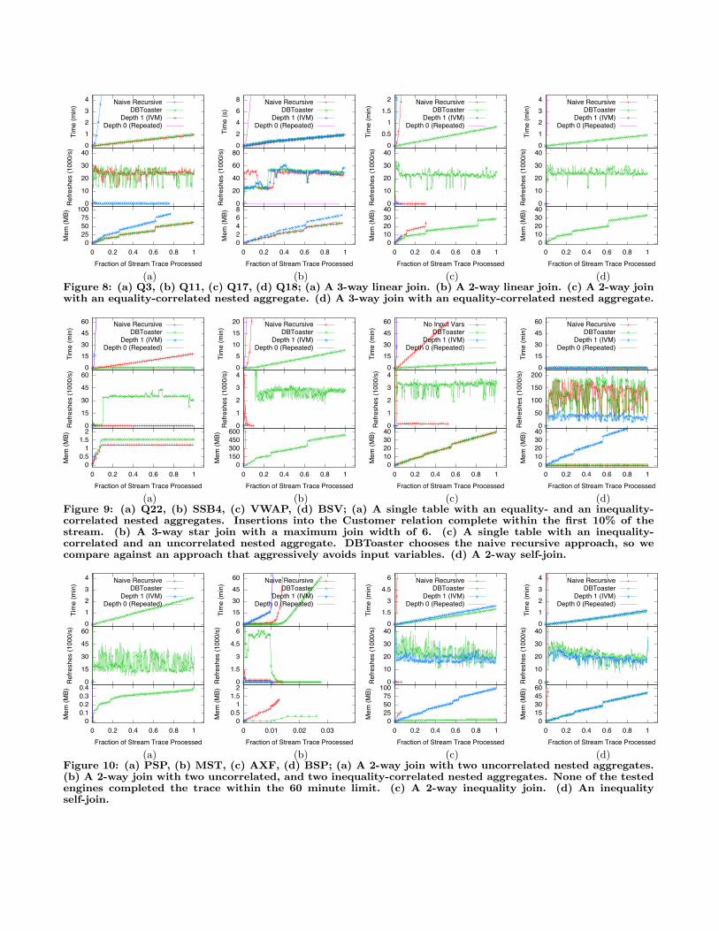
price, and a volume. The TPC-H benchmark queries Q3,Q11, Q17, Q18, Q22, and SSB4 were run on a stream of up-dates adapted from a database generated by DBGEN[31].We simulate a system that monitors a set of “active” ordersby randomly interleaving insertions on all relations and in-jecting random deletions on Orders rows to keep the Orderstable at around 30 thousand tuples. Results presented inFigures 8, 9 and 10 are based on a scaling factor 0.1 (100MB) database. We show that these results scale to longerstreams in Section 6.2.

To evaluate our compilation algorithm, DBToaster pro-duces three alternatives by terminating recursive compila-tion early. Depth 0 compilation corresponds to re-evaluatingthe query on every update, while compilation at Depth 1 isclassical first-order IVM. As the third option, DBToastermaterializes as much of the query as possible (Naive Re-cursive), creating view caches and employing partial mate-rialization to decorrelate nested subqueries. Our resultsshow the number of tuples processed by queries run over areplayed stream for a 1 hour period.

6.1 Higher-Order IVM PerformanceWe now analyze the steady-state performance of DBToaster.Comparison with Commercial Systems. Figure 7 com-pares higher-order IVM to the performance of a commer-cial DBMS (DBX) and stream processor (SPY), anonymizeddue to their license agreements. We present a summary ofour findings, an in-depth itemized breakdown of overheadsis outside the scope of this paper. SPY does not supportIVM, so the number presented is for full re-evaluation of thequery on every update. For nested queries, our workload uti-lizes SPY’s in-memory tables which significantly contributesto the performance gap from DBToaster due to their syn-chronization requirements in an asynchronous stream en-

0 1 2 3 4

Tim

e (m

in) Naive Recursive

DBToasterDepth 1 (IVM)

Depth 0 (Repeated)

0

10

20

30

40

Ref

resh

es (1

000/

s)

0 25 50 75

100

0 0.2 0.4 0.6 0.8 1

Mem

(MB)

Fraction of Stream Trace Processed

0 2 4 6 8

Tim

e (s

)

Naive RecursiveDBToaster

Depth 1 (IVM)Depth 0 (Repeated)

0

20

40

60

80

Ref

resh

es (1

000/

s)

0 2 4 6 8

0 0.2 0.4 0.6 0.8 1

Mem

(MB)


0 0.5

1 1.5

2

Tim

e (m

in) Naive Recursive


Depth 0 (Repeated)

0

10

20

30

40

Ref

resh

es (1

000/

s)

0 10 20 30 40

0 0.2 0.4 0.6 0.8 1

Mem

(MB)


0 1 2 3 4

Tim

e (m

in) Naive Recursive


Depth 0 (Repeated)

0

10

20

30

40

Ref

resh

es (1

000/

s)

0 10 20 30 40

0 0.2 0.4 0.6 0.8 1

Mem

(MB)


(a) (b) (c) (d)Figure 8: (a) Q3, (b) Q11, (c) Q17, (d) Q18; (a) A 3-way linear join. (b) A 2-way linear join. (c) A 2-way joinwith an equality-correlated nested aggregate. (d) A 3-way join with an equality-correlated nested aggregate.

0 15 30 45 60

Tim

e (m

in) Naive Recursive


Depth 0 (Repeated)

0

15

30

45

60

Ref

resh

es (1

000/

s)

0 0.5

1 1.5

2

0 0.2 0.4 0.6 0.8 1

Mem

(MB)


0 5

10 15 20

Tim

e (m

in) Naive Recursive


Depth 0 (Repeated)

0

1

2

3

4

Ref

resh

es (1

000/

s)

0 150 300 450 600

0 0.2 0.4 0.6 0.8 1

Mem

(MB)


0 15 30 45 60

Tim

e (m

in) No Input Vars


Depth 0 (Repeated)

0

1

2

3

4R

efre

shes

(100

0/s)

0 10 20 30 40

0 0.2 0.4 0.6 0.8 1

Mem

(MB)


0 15 30 45 60

Tim

e (m

in) Naive Recursive


Depth 0 (Repeated)

0

50

100

150

200

Ref

resh

es (1

000/

s)

0 10 20 30 40

0 0.2 0.4 0.6 0.8 1

Mem

(MB)


(a) (b) (c) (d)Figure 9: (a) Q22, (b) SSB4, (c) VWAP, (d) BSV; (a) A single table with an equality- and an inequality-correlated nested aggregates. Insertions into the Customer relation complete within the first 10% of thestream. (b) A 3-way star join with a maximum join width of 6. (c) A single table with an inequality-correlated and an uncorrelated nested aggregate. DBToaster chooses the naive recursive approach, so wecompare against an approach that aggressively avoids input variables. (d) A 2-way self-join.

0 1 2 3 4

Tim

e (m

in) Naive Recursive


Depth 0 (Repeated)

0

15

30

45

60

Ref

resh

es (1

000/

s)

0 0.1 0.2 0.3 0.4

0 0.2 0.4 0.6 0.8 1

Mem

(MB)


0 15 30 45 60

Tim

e (m

in) Naive Recursive


Depth 0 (Repeated)

0

1.5

3

4.5

6

Ref

resh

es (1

000/

s)

0 0.5

1 1.5

2

0 0.01 0.02 0.03

Mem

(MB)


0 1.5

3 4.5

6

Tim

e (m

in) Naive Recursive


Depth 0 (Repeated)

0

10

20

30

40

Ref

resh

es (1

000/

s)

0 25 50 75

100

0 0.2 0.4 0.6 0.8 1

Mem

(MB)


0 1 2 3 4

Tim

e (m

in) Naive Recursive


Depth 0 (Repeated)

0

10

20

30

40

Ref

resh

es (1

000/

s)

0 15 30 45 60

0 0.2 0.4 0.6 0.8 1

Mem

(MB)


(a) (b) (c) (d)Figure 10: (a) PSP, (b) MST, (c) AXF, (d) BSP; (a) A 2-way join with two uncorrelated nested aggregates.(b) A 2-way join with two uncorrelated, and two inequality-correlated nested aggregates. None of the testedengines completed the trace within the 60 minute limit. (c) A 2-way inequality join. (d) An inequalityself-join.

gine. For DBX, although this does support IVM, more thanhalf of the queries in our test workload require features ofSQL that cannot be handled incrementally by DBX’s viewssubsystem. In our experiments, we found two significantcontributors to DBX’s overheads. First, because DBX onlyperforms IVM after commits, transaction overheads greatlyadd to the cost of achieving fast refresh. Second, maintain-ing catalog information across many tables for high-rate up-dates also substantially impacts latencies and throughput.Equijoins. Q3 and Q11 (Figure 8a,b) are 2- and 3-way lin-ear joins respectively, SSB4 (Figure 9b) is a 3-way star joinwith a maximum join-width of 6, and BSV (Figure 9d) isa 2-way self-join. As there are no inequalities, DBToasterand Naive Recursive Compilation produce mostly identicalresults. In the case of many 2-way joins, the first level deltasare very nearly the base relations, and so on Q11, IVM isable to perform as effectively as DBToaster. On BSV how-ever, DBToaster gets a substantial performance improve-ment by representing the materialized delta view with onlya single aggregate value, making the update cost constant.SSB4 normally has a join width of 6. However, because thecontents of the Nation table are static, DBToaster does notattempt to materialize any deltas needed to support updatesto Nation, reducing the join width to 4 and eliminating sev-eral maps with high maintenance costs.Nested Aggregates. Q17 and Q18 (Figure 8c,d) are multi-way join nested-aggregate queries with simple nested aggre-gates, in both case with the nested aggregate correlated onan equality. Here, DBToaster’s strong performance comesfrom decorrelating the nested subquery for only the deltasof Lineitem (on which both nested subqueries are based).

Q22 (Figure 9a) includes two nested aggregates, an uncor-related aggregate on Customer that is compared against onthe top level using an inequality and an equality-correlatedaggregate on Orders that is compared against using an in-equality. The first nested subquery causes DBToaster tochoose a strategy of re-evaluating the top-level query sincethe delta of the subquery with respect to updates to Cus-tomer is not simpler than the original subquery. The secondsubquery by itself would not have made this necessary sincewe can decorrelate it (due to the absence of both inequalitiesand the Customer relation) and avoid input variables in anyquery subexpression. Nevertheless, the two subqueries aswell as the top-level aggregation without the inequality canbe materialized, reducing re-evaluation to a loop over na-tions. This is seen in the performance graph as the query’sslow startup ends once the last customer has been inserted.

VWAP (Figure 9c) has a nested aggregate correlated onan inequality. The small domain of the correlation variable(price) makes this an ideal candidate for view caching.

PSP (Figure 10a) has two uncorrelated nested aggregates.This query benefits from full re-evaluation on each execu-tion. However, polynomial expansion actually enables agraph decomposition that splits the query into 4 parts: 2constant time components and 2 independent linear timecomponents in the number of distinct values of the columnbeing compared to the nested aggregate (volume).

MST (Figure 10b) is fundamentally similar to PSP, butrather than comparing its uncorrelated aggregates againstcolumns from the base relations, they are each comparedagainst another nested aggregate correlated on an inequality.This is a worst case scenario for DBToaster, as it cannotincrementally process this query in better than O(n2) timewithout specialized indexes (e.g., aggregate range trees).Inequijoins. AXF and BSP are both 2-way joins (Figure10c,d), with BSP being a self-join. In the case of AXF, boththe join variable (price) and one of the aggregate variables(volume) are treated as input variables by naive recursive

0

0.2

0.4

0.6

0.8

1

1.2

1.4

Q3 Q11 Q17 Q18 Q22 SSB4

Ref

resh

Rat

e R

elat

ive

to 1

00 M

B 100 MB500 MB

1 GB5 GB

10 GB

Figure 11: Performance scaling on the TPCH queries.

materialization. In BSP, the join variable (t) has an ex-tremely large domain. In both cases, partial materializationoutperforms naive. Since both are 2-way joins, IVM is nearlyoptimal – DBToaster achieves a small speed boost in bothcases by not materializing the entire base relation.

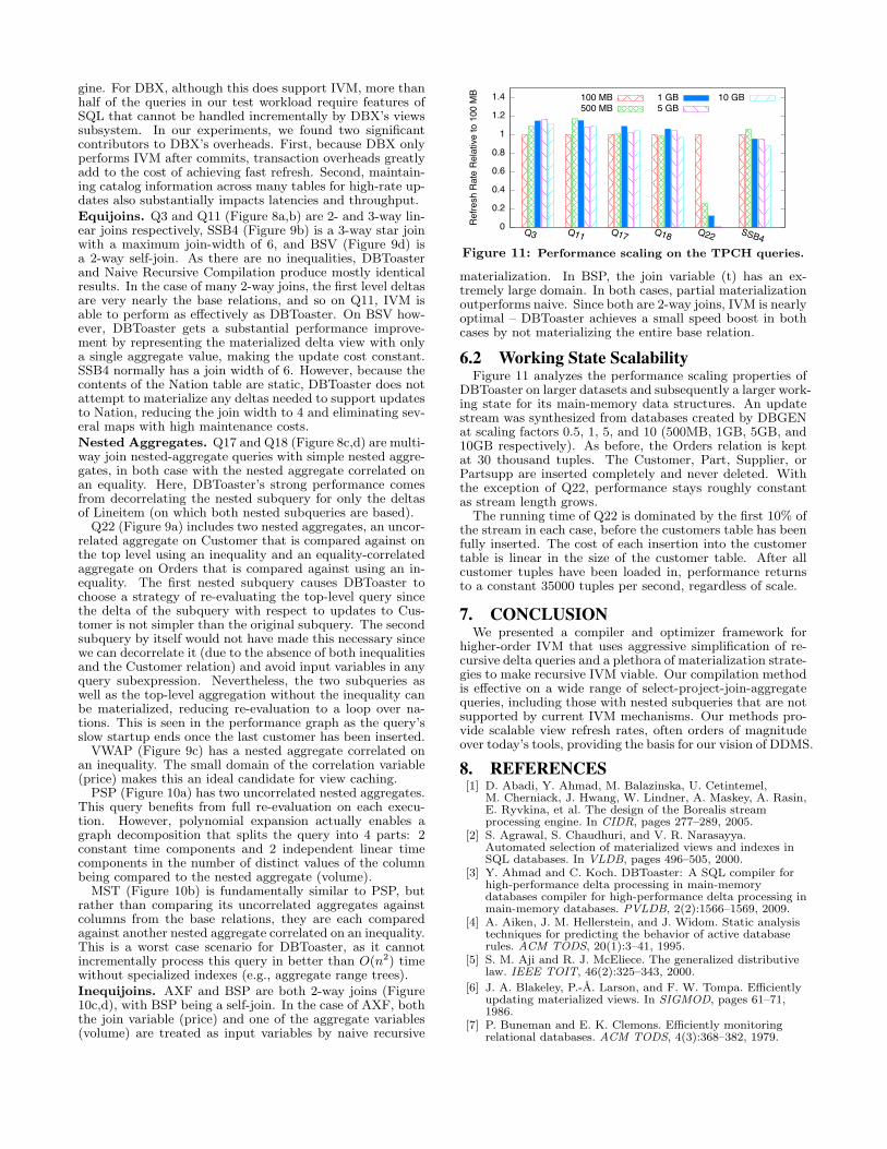
6.2 Working State ScalabilityFigure 11 analyzes the performance scaling properties of

DBToaster on larger datasets and subsequently a larger work-ing state for its main-memory data structures. An updatestream was synthesized from databases created by DBGENat scaling factors 0.5, 1, 5, and 10 (500MB, 1GB, 5GB, and10GB respectively). As before, the Orders relation is keptat 30 thousand tuples. The Customer, Part, Supplier, orPartsupp are inserted completely and never deleted. Withthe exception of Q22, performance stays roughly constantas stream length grows.

The running time of Q22 is dominated by the first 10% ofthe stream in each case, before the customers table has beenfully inserted. The cost of each insertion into the customertable is linear in the size of the customer table. After allcustomer tuples have been loaded in, performance returnsto a constant 35000 tuples per second, regardless of scale.

7. CONCLUSIONWe presented a compiler and optimizer framework for

higher-order IVM that uses aggressive simplification of re-cursive delta queries and a plethora of materialization strate-gies to make recursive IVM viable. Our compilation methodis effective on a wide range of select-project-join-aggregatequeries, including those with nested subqueries that are notsupported by current IVM mechanisms. Our methods pro-vide scalable view refresh rates, often orders of magnitudeover today’s tools, providing the basis for our vision of DDMS.

8. REFERENCES[1] D. Abadi, Y. Ahmad, M. Balazinska, U. Cetintemel,

M. Cherniack, J. Hwang, W. Lindner, A. Maskey, A. Rasin,E. Ryvkina, et al. The design of the Borealis streamprocessing engine. In CIDR, pages 277–289, 2005.

[2] S. Agrawal, S. Chaudhuri, and V. R. Narasayya.Automated selection of materialized views and indexes inSQL databases. In VLDB, pages 496–505, 2000.

[3] Y. Ahmad and C. Koch. DBToaster: A SQL compiler forhigh-performance delta processing in main-memorydatabases compiler for high-performance delta processing inmain-memory databases. PVLDB, 2(2):1566–1569, 2009.

[4] A. Aiken, J. M. Hellerstein, and J. Widom. Static analysistechniques for predicting the behavior of active databaserules. ACM TODS, 20(1):3–41, 1995.

[5] S. M. Aji and R. J. McEliece. The generalized distributivelaw. IEEE TOIT, 46(2):325–343, 2000.

[6] J. A. Blakeley, P.-A. Larson, and F. W. Tompa. Efficientlyupdating materialized views. In SIGMOD, pages 61–71,1986.

[7] P. Buneman and E. K. Clemons. Efficiently monitoringrelational databases. ACM TODS, 4(3):368–382, 1979.

[8] S. Chaudhuri, R. Krishnamurthy, S. Potamianos, andK. Shim. Optimizing queries with materialized views. InICDE, pages 190–200, 1995.

[9] L. S. Colby, T. Griffin, L. Libkin, I. S. Mumick, andH. Trickey. Algorithms for deferred view maintenance. InSIGMOD, pages 469–480, 1996.

[10] L. S. Colby, A. Kawaguchi, D. F. Lieuwen, I. S. Mumick,and K. A. Ross. Supporting multiple view maintenancepolicies. In SIGMOD, pages 405–416, 1997.

[11] G. Cormode and S. Muthukrishnan. What’s hot and what’snot: Tracking most frequent items dynamically. ACM

TODS, 30(1):249–278, 2005.[12] U. Dayal, N. Goodman. Query optimization for CODASYL

database systems. In SIGMOD, pages 138–150, 1982.[13] T. M. Ghanem, A. K. Elmagarmid, P.-A. Larson, and

W. G. Aref. Supporting views in data stream managementsystems. ACM TODS, 35(1):1–47, 2010.

[14] T. Griffin and L. Libkin. Incremental maintenance of viewswith duplicates. In SIGMOD, pages 328–339, 1995.

[15] A. Gupta, I. S. Mumick, V. S. Subrahmanian. Maintainingviews incrementally. In SIGMOD, pages 157–166, 1993.

[16] H. Gupta and I. S. Mumick. Selection of views tomaterialize in a data warehouse. IEEE TKDE, 17(1):24–43,2005.

[17] A. Kawaguchi, D. F. Lieuwen, I. S. Mumick, and K. A.Ross. Implementing incremental view maintenance innested data models. In DBPL, pages 202–221, 1997.

[18] O. Kennedy, Y. Ahmad, and C. Koch. DBToaster: Agileviews for a dynamic data management system. In CIDR,pages 284–295, 2011.

[19] C. Koch. Incremental query evaluation in a ring ofdatabases. In PODS, pages 87–98, 2010.

[20] Y. Kotidis and N. Roussopoulos. A case for dynamic viewmanagement. ACM TODS, 26(4):388–423, 2001.

[21] S. Krishnamurthy, C. Wu, and M. J. Franklin. On-the-flysharing for streamed aggregation. In SIGMOD, pages623–634, 2006.

[22] P.-A. Larson and J. Zhou. Efficient maintenance ofmaterialized outer-join views. In ICDE, pages 56–65, 2007.

[23] Y. A. Liu, S. D. Stoller, and T. Teitelbaum. Static cachingfor incremental computation. ACM TOPLAS,20(3):546–585, 1998.

[24] R. Motwani, J. Widom, et. al. Query processing,approximation, and resource management in a data streammanagement system. In CIDR, 2003.

[25] T. Palpanas, R. Sidle, R. Cochrane, and H. Pirahesh.Incremental maintenance for non-distributive aggregatefunctions. In VLDB, pages 802–813, 2002.

[26] B. A. Pearlmutter and J. M. Siskind. Lazy multivariatehigher-order forward-mode AD. In POPL, pages 155–160,2007.

[27] K. A. Ross, D. Srivastava, and S. Sudarshan. Materializedview maintenance and integrity constraint checking:Trading space for time. In SIGMOD, pages 447–458, 1996.

[28] N. Roussopoulos. An incremental access method forViewCache: Concept, algorithms, and cost analysis. ACM

TODS, 16(3):535–563, 1991.[29] K. Salem, K. S. Beyer, R. Cochrane, and B. G. Lindsay.

How to roll a join: Asynchronous incremental viewmaintenance. In SIGMOD, pages 129–140, 2000.

[30] N. Tatbul, U. Cetintemel, S. B. Zdonik, M. Cherniack, andM. Stonebraker. Load shedding in a data stream manager.In VLDB, pages 309–320, 2003.

[31] Transaction Processing Performance Council. TPC-Hbenchmark specification. http://www.tpc.org/hspec.html.

[32] S. D. Viglas and J. F. Naughton. Rate-based queryoptimization for streaming information sources. InSIGMOD, pages 37–48, 2002.

[33] J. Yang and J. Widom. Incremental computation andmaintenance of temporal aggregates. VLDB Journal,12(3):262–283, 2003.

[34] J. Zhou, P.-A. Larson, H. G. Elmongui. Lazy maintenanceof materialized views. In VLDB, pages 231–242, 2007.

[35] J. Zhou, P.-A. Larson, J. C. Freytag, and W. Lehner.Efficient exploitation of similar subexpressions for queryprocessing. In SIGMOD, pages 533–544, 2007.

[36] D. C. Zilio, C. Zuzarte, S. Lightstone, W. Ma, G. M.Lohman, R. Cochrane, H. Pirahesh, L. S. Colby, J. Gryz,E. Alton, D. Liang, and G. Valentin. Recommendingmaterialized views and indexes with IBM DB2 designadvisor. In ICAC, pages 180–188, 2004.

Appendix A. QUERIES

AX

F SELECT b.broker_id, sum(a.volume-b.volume)FROM Bids b, Asks aWHERE b.broker_id = a.broker_id

AND (a.price-b.price > 1000 OR b.price-a.price > 1000)GROUP BY b.broker_id;

BSP SELECT x.broker_id, sum(x.volume*x.price - y.volume*y.price)

FROM Bids x, Bids yWHERE x.broker_id=y.broker_id AND x.t>y.tGROUP BY x.broker_id;

BSV SELECT x.broker_id, sum(x.volume*x.price*y.volume*y.price*0.5)

FROM Bids x, Bids yWHERE x.broker_id = y.broker_id GROUP BY x.broker_id;

MST SELECT b.broker_id, sum(a.price*a.volume - b.price*b.volume)

FROM Bids b, Asks aWHERE 0.25*(select sum(a1.volume) from Asks a1) >

(select sum(a2.volume) from Asks a2 where a2.price>a.price)AND 0.25*(select sum(b1.volume) from Bids b1) >

(select sum(b2.volume) from Bids b2 where b2.price>b.price)GROUP BY b.broker_id;

PSP SELECT sum(a.price - b.price) FROM Bids b, Asks a

WHERE b.volume>0.0001*(select sum(b1.volume) from Bids b1)AND a.volume>0.0001*(select sum(a1.volume) from Asks a1);

VW

AP SELECT sum(b1.price * b1.volume) FROM Bids b1

WHERE 0.25 * (select sum(b3.volume) from Bids b3) >(select sum(b2.volume) from Bids b2where b2.price>b1.price);

Q3 SELECT o.orderkey, o.orderdate, o.shippriority,

sum(li.extendedprice * (1 - li.discount))FROM Customer c, Orders o, Lineitem liWHERE c.mktsegment = ’BUILDING’

AND o.custkey = c.custkeyAND li.orderkey = o.orderkeyAND o.orderdate < DATE(’1995-03-15’)AND li.shipdate > DATE(’1995-03-15’)

GROUP BY o.orderkey, o.orderdate, o.shippriority;

Q11 SELECT ps.partkey, sum(ps.supplycost * ps.availqty)

FROM Partsupp ps, Supplier sWHERE ps.suppkey = s.suppkey GROUP BY ps.partkey;

Q17 SELECT sum(l.extendedprice) FROM Lineitem l, Part pWHERE p.partkey = l.partkeyAND l.quantity < 0.005 * (select sum(l2.quantity)

from Lineitem l2 where l2.partkey = p.partkey);

Q18 SELECT c.custkey, sum(l1.quantity)

FROM Customer c, Orders o, Lineitem l1WHERE 1 <= (select sum(1) where

100 < (select sum(l2.quantity) from Lineitem l2where l1.orderkey = l2.orderkey))

AND c.custkey = o.custkey AND o.orderkey = l1.orderkeyGROUP BY c.custkey;

Q22 SELECT c1.nationkey, sum(c1.acctbal) FROM Customer c1

WHERE c1.acctbal <(select sum(c2.acctbal) from Customer c2 where c2.acctbal>0)

AND 0=(select sum(1) from Orders o where o.custkey=c1.custkey)GROUP BY c1.nationkey;

SSB

4 SELECT sn.regionkey, cn.regionkey, p.type,sum(li.quantity)

FROM Customer c, Orders o, Lineitem li,Part p, Supplier s, Nation cn, Nation sn

WHERE c.custkey = o.custkeyAND o.orderkey = li.orderkeyAND p.partkey = li.partkeyAND s.suppkey = li.suppkeyAND o.orderdate >= DATE(’1997-01-01’)AND o.orderdate < DATE(’1998-01-01’)AND cn.nationkey = c.nationkeyAND sn.nationkey = s.nationkey

GROUP BY sn.regionkey, cn.regionkey, p.type;

higher-order delta processing for dynamic, frequently fresh views

Documents