higher order expectations, illiquidity, and short …...iese business school-university of navarra...
TRANSCRIPT

IESE Business School-University of Navarra - 1
HIGHER ORDER EXPECTATIONS, ILLIQUIDITY, AND SHORT-TERM
TRADING
Giovanni Cespa
Xavier Vives
IESE Business School – University of Navarra Av. Pearson, 21 – 08034 Barcelona, Spain. Phone: (+34) 93 253 42 00 Fax: (+34) 93 253 43 43 Camino del Cerro del Águila, 3 (Ctra. de Castilla, km 5,180) – 28023 Madrid, Spain. Phone: (+34) 91 357 08 09 Fax: (+34) 91 357 29 13 Copyright © 2011 IESE Business School.
Working Paper
WP-915
March, 2011

IESE Business School-University of Navarra
The Public-Private Sector Research Center is a Research Center based at IESE Business School. Its mission is to develop research that analyses the relationships between the private and public sectors primarily in the following areas: regulation and competition, innovation, regional economy and industrial politics and health economics.
Research results are disseminated through publications, conferences and colloquia. These activities are aimed to foster cooperation between the private sector and public administrations, as well as the exchange of ideas and initiatives.
The sponsors of the SP-SP Center are the following:
Accenture Ajuntament de Barcelona Caixa Manresa Cambra Oficial de Comerç, Indústria i Navegació de Barcelona Departament d’ Economia i Coneixement de la Generalitat de Catalunya Departament d’ Empresa i Ocupació de la Generalitat de Catalunya Diputació de Barcelona Endesa FOBSIC Fundació AGBAR Institut Català de les Indústries Culturals Mediapro Sanofi Aventis ATM, FGC y TMB
The contents of this publication reflect the conclusions and findings of the individual authors, and not the opinions of the Center's sponsors.

IESE Business School-University of Navarra
HIGHER ORDER EXPECTATIONS, ILLIQUIDITY, AND SHORT-TERM
TRADING
Giovanni Cespa1
Xavier Vives2
Abstract We propose a theory that jointly accounts for an asset illiquidity and for the asset price potential over-reliance on public information. We argue that, when trading frequencies differ across traders, asset prices reflect investors' Higher Order Expectations (HOEs) about the two factors that influence the aggregate demand: fundamentals information and liquidity trades. We show that it is precisely when asset prices are driven by investors' HOEs about fundamentals that they over-rely on public information, the market displays high illiquidity, and low volume of informational trading; conversely, when HOEs about fundamentals are subdued, prices under-rely on public information, the market hovers in a high liquidity state, and the volume of informational trading is high. Over-reliance on public information results from investors' under-reaction to their private signals which, in turn, dampens uncertainty reduction over liquidation prices, favoring an increase in price risk and illiquidity. Therefore, a highly illiquid market implies higher expected returns from contrarian strategies. Equivalently, illiquidity arises as a byproduct of the lack of participation of informed investors in their capacity of liquidity suppliers, a feature that appears to capture some aspects of the recent crisis. Keywords: Expected returns, multiple equilibria, average expectations, over-reliance on public information, Beauty Contest. JEL Classification Numbers: G10, G12, G14
We thank Marcelo Fernandes, Peter Kondor, Ioanid Rosu, and seminar participants in the Econometrics Workshop at Queen Mary University of London, the 2010 European Finance Association meeting (Frankfurt), the ELSE-UCL Workshop in Financial Economics (UCL, September 2010), and the IESEG workshop on Asset Pricing (IESEG, May 2010) for their comments. 1 Cass Business School, CSEF, and CEPR. 2 Professor of Economics, Abertis Chair of Regulation, Competition and Public Policy, IESE. The research leading to these results has received funding from the European Research Council under the European Advanced Grants scheme, Grant Agreement no. 230254. I also thank the support of project ECO2008-05155 of the Spanish Ministry of Education and Science at the Public-Private Sector Research Center at IESE.

1 Introduction
Liquidity plays an important role in the valuation of financial assets.1 A relevant aspect of
liquidity relates to the provision of immediacy, i.e. investors’ readiness to hold a position
in an asset in order to bridge the offsetting needs of agents who enter the market at different
points in time (Grossman and Miller (1988)). A higher uncertainty over the price at which asset
inventories can be unwound creates inventory risk, thereby reducing investors’ ability to provide
immediacy, and curtailing liquidity.2 In markets with heterogeneous information, the risk of
facing adverse selection at interim liquidation dates adds to inventory risk, potentially further
increasing illiquidity. When prices reflect more efficiently the fundamentals, adverse selection
is less of an issue, as the speculative opportunities offered by private information are scarcer.
Price efficiency, in turn, hinges on investors’ responses to their private signals. This implies
that in equilibrium, both market illiquidity and investors’ response to private information are
jointly determined. Equivalently, illiquidity must proxy for the amount of information that,
via equilibrium prices, investors transmit to the market.
The impact of private information on asset prices is also at the core of the recent literature
that emphasises the role of investors’ Higher Order Expectations (HOEs) over asset payoffs
in asset price determination (i.e., investors’ expectations about other investors’ expectations
about . . . the liquidation value). It is a basic tenet of this literature that if prices are driven
by HOEs over the final payoff, they over-rely on public information, systematically departing
from fundamentals compared to consensus (Allen, Morris, and Shin (2006)). While this result
speaks to the informational properties of asset prices, it is less clear what its implications for
market quality are.
In this paper we propose a theory that jointly accounts for an asset illiquidity and for
the asset price potential over-reliance on public information. We argue that in general asset
prices reflect investors’ HOEs about the two factors that influence the aggregate demand:
fundamentals and liquidity trades. We show that it is precisely when asset prices are driven
by investors’ HOEs about fundamentals (and therefore over-rely on public information) that
the market displays high illiquidity, and the volume of informational trading is low; conversely,
when HOEs about fundamentals are subdued, asset prices under-rely on public information, the
market hovers in a high liquidity state, and the volume of informational trading is high. Over-
reliance on public information results from investors’ under-reaction to their private signals
which, in turn, dampens uncertainty reduction over liquidation prices, favoring an increase in
adverse selection risk and illiquidity. Therefore, a highly illiquid market implies higher expected
returns from contrarian strategies. Equivalently, illiquidity arises as a byproduct of the lack of
participation of informed investors in their capacity of liquidity suppliers, a feature that seems
to capture some aspects of the recent crisis (see, e.g. Distaso, Fernandes, and Zikes (2010) and
Nagel (2010)).
1There is by now a well established literature showing that illiquid assets command a return premium (see,e.g., Pastor and Stambaugh (2003), and Acharya and Pedersen (2005)).
2Several authors document intermediarys’ concern over the time-varying patterns of asset illiquidity. Seee.g. Comerton-Forde, Hendershott, Jones, Moulton, and Seasholes (2010).
2

More in detail, we study a market in which overlapping generations of risk-averse, rational
investors interact with liquidity traders. The former live for two periods and are informed
about a pay-off that will be announced at a future date, which occurs beyond their investment
horizon; the latter, instead, are uninformed and submit a random market order, potentially
holding their positions during more than one trading round. When young, rational investors
absorb liquidity traders’ orders, thereby acting as “market-makers.” Once old, the former
unwind their positions against the reverting portion of the latter demand and take advantage
of the new cohort of rational investors to unload the residual part of their inventory. Thus, as
trading frequencies are heterogenous across investors’ types, rational investors provide liquidity
when young and consume it when old. This implies that when they determine their holdings,
they take into account the inventory and adverse selection risk they will face at the liquidation
date. We show that this feature of the model generates a number of important implications.
If in a given period rational investors anticipate that their next period peers will increase
their exposure to the risky asset, they face adverse selection risk at the liquidation date which
will make the market more illiquid. As a consequence, the price at which they unwind becomes
more difficult to forecast with their private signal, and they scale down their response to private
information. This, in turn, lowers the informativeness of equilibrium prices, opening more
opportunities to speculate on private information to the informed investors who enter the
market in the following period, justifying the anticipated increase in illiquidity. If, on the other
hand, in a given period investors anticipate that their next period peers lower their exposure
to the risky asset, the market in which they unwind will be more liquid. As a consequence,
the liquidation price becomes more easy to forecast with their information, and they step up
the use of private signals. This, in turn, increases the informativeness of equilibrium prices,
reducing the opportunities to speculate on private information opened to the next generation
of informed investors, justifying the anticipated decrease in illiquidity. We thus show that the
presence of such a positive feedback loop across trading dates is conducive to multiple equilibria
which can be ranked in terms of illiquidity.
As rational investors hold disparate signals, the illiquidity result also has implications for the
information aggregation properties of asset prices. Differently from the existing literature, we
show that in our setup the occurrence of over-reliance on public information is closely related
to the type of equilibrium that arises. Along the equilibrium in which investors anticipate
high future illiquidity, the risk of adverse price movements at the time of position unwinding
causes over-reaction to public information; this generates a price that is poorly related to
fundamentals. Conversely, when investors anticipate low future illiquidity, the price under-
reacts to public information and tracks more closely the fundamentals. Thus, while HOEs over
fundamentals are necessary for over-reaction to public information, they are not sufficient.
The existence of multiple equilibria leaves open the question of which equilibrium is more
likely to arise. As our intuitive argument has clarified, in our setup multiple equilibria rely on
the positive feedback loop that links investors’ response to private information in a given period
to the illiquidity of the following period market. Thus, any effect that moderates such a loop is
3

likely to restore uniqueness. With this idea in mind we show that when either liquidity traders’
demand becomes transient or when a spike in the residual uncertainty affecting fundamentals
hits the market, a unique equilibrium arises. In this equilibrium the market is more illiquid
and prices always over-react to public information. Indeed, when agents’ liquidity needs are
fully synchronized, the cohort of rational investors who enters the market in a given period
anticipates that liquidity traders will completely revert their position in the following period,
providing the natural counterpart to their position unwinding. This, in turn, reduces the need
to anticipate the liquidation price, and enforces an equilibrium in which rational investors over-
react to public information.3 Similarly, when fundamentals uncertainty spikes, asset prices
increasingly reflect liquidity shocks and rational investors have little use for their signals. In
both cases, thus, it is the possibility to focus on servicing the needs of liquidity traders that
“distracts” rational investors from forecasting the fundamentals, yielding an equilibrium with
higher price risk and higher illiquidity.
Our model can shed light on the impact that heterogeneous trading frequencies have on
market liquidity. Indeed, the low illiquidity equilibrium arises precisely because when the
horizon of liquidity traders differs from the one of informed investors, the latter anticipate
a potential adverse selection risk at the liquidation date. Along this equilibrium, liquidity
traders’ losses are minimized, which leads to conclude that if they had access to the same
trading technology available to informed investors, liquidity traders would adopt it. However,
in this case as trading frequencies coincide, the adverse selection risk at the liquidation date
disappears together with the low illiquidity equilibrium. Thus, an implication of our analysis
is that while trading at high frequencies may generate liquidity improvements (as empirically
documented, for example, by Hendershott, Jones, and Menkveld (2010)), these improvements
are not necessarily exploitable by those who are to gain the most from it, namely liquidity
traders. A further implication of our model is that with differential information, the existence
of a discrepancy in the speed at which different types of investors can turn around their positions
can be responsible for indeterminacy, making liquidity dependent on a coordination problem
across different generations of investors, and thereby endogenously creating a source of liquidity
risk.
Our model also provides a theoretical underpinning for the empirically documented positive
association between illiquidity and asset expected returns.4 In fact we show that it is precisely
along the high illiquidity equilibrium that the asset expected returns are higher and rational
investors concentrate on the supply of immediacy to liquidity traders acting as “contrarians.”
If, on the other hand, price risk is low, the market is liquid, liquidity supply is not very prof-
itable (low price risk and thus low risk compensation) and investors act as “trend chasers.”
As argued above, whether price risk is high or low depends on a coordination problem and we
predict that high price risk occurs when informed investors refrain from using private infor-
3In this case our model coincides with Allen, Morris and Shin (2006).4Acharya and Pedersen (2005), estimate that low liquidity stocks command a 4.6% higher expected return
over high liquidity stocks. Brennan and Subrahmanyam (1996) find that low liquidity portfolios earn an extra6.6% yearly return over high liquidity portfolios.
4

mation exactly because prices are mainly driven by liquidity shocks which are orthogonal to
fundamentals. Therefore, our model implies that liquidity provision is profitable when there is
little informational trading in the market.
The rest of the paper is organized as follows: in the next section we review the related
literature. We spell out the model’s assumptions and analyse the model in a setting with
no private information. We then turn to the market with heterogeneous information. In
the following section we relate our illiquidity result to the literature on HOEs. We conclude
analyzing extensions and providing a discussion of our results.
2 Related literature
This paper is related to a growing literature that points out the relevance of higher order
expectations in influencing asset prices. As our previous discussion suggests, we depart from
the main tenet of this literature and point out that price over-reliance on public information is
intimately related to the transience of liquidity traders’ demand.5 Bacchetta and van Wincoop
(2008) study the role of higher order beliefs in asset prices in an infinite horizon model showing
that higher order expectations add an additional term to the traditional asset pricing equation,
the higher order “wedge,” which captures the discrepancy between the price of the asset and the
average expectations of the fundamentals. Kondor (2009), in a model with short-term Bayesian
traders, shows that public announcements may increase disagreement, generating high trading
volume in equilibrium. Nimark (2007), in the context of Singleton (1987)’s model, shows that
under some conditions both the variance and the impact that expectations have on the price
decrease as the order of expectations increases. Other authors have analyzed the role of higher
order expectations in models where traders hold different initial beliefs about the liquidation
value. Biais and Bossaerts (1998) show that departures from the common prior assumption
rationalise peculiar trading patterns whereby traders with low private valuations may decide
to buy an asset from traders with higher private valuations in the hope to resell it later on
during the trading day at an even higher price. Cao and Ou-Yang (2005) study conditions for
the existence of bubbles and panics in a model where traders’ opinions about the liquidation
value differ.6 Banerjee, Kaniel, and Kremer (2009) show that in a model with heterogeneous
priors, differences in higher order beliefs may induce price drift. Ottaviani and Sørensen (2009),
in a static model of a binary prediction market where agents hold heterogeneous prior beliefs
and are wealth constrained (either exogenously, by the rules of the market, or because of their
attitude towards risk), show that the fully revealing REE price underweights aggregate private
information.
The paper is also related to the literature that investigates the relationship between the
impact of short-term information on prices and investors’ reaction to their private signals (see,
e.g. Vives (1995), Cespa (2002), and Vives (2008) for a survey). Several authors have argued
5In a related paper, we show that a similar conclusion holds in a model with long term investors (see Cespaand Vives (2009)).
6Kandel and Pearson (1995) provide empirical evidence supporting the non-common prior assumption.
5

that when private information is related to an event which occurs beyond the date at which
investors liquidate their positions, the latter act on their signals only if they expect them to
be reflected in the price at which they liquidate (see, e.g., Dow and Gorton (1994) and Froot,
Scharfstein, and Stein (1992)). In our context the main driver in investors’ reaction to private
signals is the uncertainty over the illiquidity of the market in which they unwind their positions.
Indeed, the impossibility to pin down a particular level of future illiquidity is responsible for
investors’ over- or under-reaction to private information which in turn feeds back into different
equilibrium levels of illiquidity.
Our analysis is also related to the literature that emphasizes the impact of illiquidity on
asset prices. Amihud and Mendelson (1986) argue that the presence of an exogenous trans-
action cost due to illiquidity leads investors to anticipate higher costs when unwinding their
positions, thereby leading to an increase in the discount factor with which they evaluate the
asset payoff. Vayanos (1998) in a multi-asset model with proportional transaction costs, shows
that in equilibrium a number of counterintuitive results can arise. In our paper illiquidity arises
endogenously, as a result of investors’ uncertainty over the price at which they unwind their
positions. Furthermore, we relate illiquidity to investors’ contrarian strategies, and to the role
that HOEs about fundamentals have in driving the asset price, showing that in an illiquid
market liquidity provision is more profitable, and that prices over-rely on public information.
Finally, our paper is also related to the literature on behavioral finance (see Barberis and
Thaler (2003) for a survey). As we will argue, our setup can accommodate overreaction to
private information as well as high volumes of informational trading and low returns from
short-term trading in a model where all investors, except for liquidity traders, are free from
behavioral biases.
3 A three-period market with short term investors
Consider a three-period version of the noisy rational expectations market analyzed by Admati
(1985) where a single risky asset with liquidation value v ∼ N(v, τ−1v ), and a risk-less asset with
unitary return are traded by a continuum of risk-averse speculators in the interval [0, 1] together
with liquidity traders. At any trading date n, a cohort of of risk averse, rational investors in the
interval [0, 1] enters the market, loads a position in the risky asset which it unwinds in period
n + 1. A rational investor i has CARA preferences (denote with γ the common risk-tolerance
coefficient) and maximizes the expected utility of his short term profit πin = (pn+1−pn)xin.7 An
investor i who enters the market in period n receives a signal sin = v+εin, where εin ∼ N(0, τ−1ε ),
v and εin are independent for all i, n and error terms are also independent both across time
periods and investors. We assume an investor i who enters the market in period n observes the
past period prices up to period n−1, denoted by pn−1 ≡ {pt}n−1t=1 , and submits a linear demand
schedule (generalized limit order) to the market Xn(sin, pn−1, pn) = ansin − ϕn(pn) indicating
the desired position in the risky asset for each realization of the equilibrium price pn. The
7We assume, without loss of generality, that the non-random endowment of investors is zero.
6

constant an denotes the private signal responsiveness, while ϕn(·) is a linear function of the
equilibrium prices pn.
The stock of liquidity trades is assumed to follow an AR(1) process:
θn = βθn−1 + un, (3.1)
where un ∼ N(0, τ−1u ) is orthogonal to θn−1, and β ∈ [0, 1]. To interpret, suppose β < 1,
then at any period n > 1 four groups of agents are in the market: the n − 1-th and n-th
generations of rational investors with demands xn−1 ≡∫ 1
0xin−1di, and xn ≡
∫ 1
0xindi, a fraction
1 − β of the n − 1-th generation of liquidity traders who revert their positions, and the new
generation of liquidity traders. Considering the first two trading dates and letting ∆x2 ≡ x2−x1,∆θ2 ≡ θ2 − θ1 = u2 + (β − 1)θ1, at equilibrium this implies
x1 + θ1 = 0
∆x2 + ∆θ2 = 0⇔ x2 + βθ1 + u2 = 0.
At date 1 the first cohort of rational investors clears the share supply θ1. At date 2 a fraction
(1− β)θ1 of the trades initiated by liquidity traders at time 1 reverts. Hence, period 1 rational
investors clear the complementary fraction βθ1 = −βx1 against the new aggregate demand:
x2 + u2. In general, the lower is β, the higher is the fraction of period n liquidity traders who
revert their positions at time n + 1, and the lower is the fraction of rational investors’ trades
that are cleared against the n+ 1-th aggregate demand. 8
Besides capturing an empirically documented feature of the demand of liquidity traders
(see, e.g., Easley et al. (2008)), assuming persistence in liquidity trades allows to model in a
parsimonious way the possibility that agents in the market have different horizons: when β = 0
each generation of rational investors and liquidity traders have the same investment horizon; as
β grows, investment horizons become increasingly different. Different investment horizons can
be justified on grounds of asynchronous liquidity needs, or of differential access to a trading
technology. Accordingly, as we will argue in section 8.1, informed investors can be seen as
high frequency traders that are able to turn around their positions at a faster speed compared
to liquidity traders. Table 1 displays the evolution of liquidity trades and rational investors’
positions in the three periods.9
We denote by Ein[Y ] = E[Y |sin, pn], En[Y ] = E[Y |pn] (Varin[Y ] = Var[Y |sin, pn], Varn[Y ] =
Var[Y |pn]), respectively the expectation (variance) of the random variable Y formed by a trader
conditioning on the private and public information he has at time n, and that obtained condi-
tioning on public information only. The consensus opinion about the fundamentals at time
n is denoted by En[v] ≡∫ 1
0Ein[v]di =
∫ 1
0Ein[v]di. Finally, we let αEn = τ ε/τ in, where
8The AR(1) assumption for liquidity traders’ demand is not new in the literature. For instance, He andWang (1995) consider a model with long term investors in which liquidity trading is generated by an AR(1)process.
9For a sufficiently large number of trading rounds N , the stock of liquidity trades reverts completely. Indeed,according to the table, at any generic time N the fraction of the first period stock of liquidity that has revertedis given by θ1(1− β)
∑N−2t=0 βt = (1− βN−1)θ1 → θ1 as N grows large.
7

Trading Date 1 2 3
Liquidity traders
Position θ1 = u1 θ2 = βθ1 + u2 θ3 = β(βθ1 + u2) + u3
Holding − βθ1 β(βθ1 + u2)
New shock u1 u2 u3
Reverting − (1− β)θ1 (1− β)(βθ1 + u2)
Rational investorsPosition x1 x2 x3
Reverting − x1 x2
Table 1: The evolution of liquidity trades and rational investors’ positions in the three periods.The position of liquidity traders in every period is given by the sum of “Holding” and “Newshock.”
τ in ≡ (Varin[v])−1 and make the convention that, given v, at any time n the average sig-
nal∫ 1
0sindi equals v almost surely (i.e. errors cancel out in the aggregate:
∫ 1
0εindi = 0).
Therefore, we have Ein[v] = αEnsin + (1− αEn)En[v], and En[v] = αEnv + (1− αEn)En[v].
4 The market without private information
In this section we assume away private information (i.e., we impose τ εn = 0). In this case,
rational investors can perfectly observe the stock of liquidity trades and always act as market
makers, providing immediacy as in Grossman and Miller (1988). It is then possible to show
that
Proposition 1. In the market without private information, there exists a unique equilibrium
in linear strategies where for n = 1, 2, 3:
Xn(θn) = −θn (4.1)
pn = v + Λnθn, (4.2)
and for n = 1, 2:
Λn =Varn[pn+1]
γ+ βΛn+1, (4.3)
while Λ3 = (γτ v)−1.
Proof. See the appendix. 2
According to (4.1) and (4.2), rational investors always take the other side of the order flow,
buying the asset at a discount when θn < 0 and selling it at a premium otherwise. Indeed, as
demand shocks are only driven by liquidity trading, rational investors anticipate return reversal
and profit from the supply of immediacy to liquidity traders:
pn+1 − pn = Λn+1un+1 + (βΛn+1 − Λn) θn
= Λn+1un+1 −Varn[pn+1]
γθn. (4.4)
8

The larger is the stock of liquidity trades θn, the larger is the adjustment in the price rational
investors require in order to absorb it. Therefore, the price impact of trades Λn proxies for the
illiquidity of the market. A higher price risk increases illiquidity and also investors’ expected
profits, as one can see by taking the expectation of (4.4):
En[pn+1 − pn] = −Varn[pn+1]
γθn. (4.5)
According to (4.3), at any time n < 3, market illiquidity captures two effects, both of
which are related to the inventory risk due to liquidity traders’ demand. On the one hand,
due to the randomness of liquidity trades, investors bear the risk related to the price at which
they will unwind their position; on the other hand, due to the persistence of liquidity traders’
demand, they anticipate the impact that the unwinding of a fraction of their holdings to the
next cohort of rational investors will have on the next period price as a result of the increased
risk exposure this implies for the next cohort of rational investors. The former effect is reflected
in the conditional variance of the liquidation price (scaled by risk tolerance) Varn[pn+1]/γ; the
latter, is instead captured by the anticipated illiquidity component βΛn+1.
More persistent liquidity trades imply a stronger effect due to investors’ position unwinding.
This, in turn, pushes investors to adjust more harshly the price for a given realization of liquidity
traders’ demand: 10
Corollary 1. In the market with homogeneous information ∂Λn/∂β > 0, for n = 1, 2.
5 The market with heterogeneous information
With heterogeneous information, the aggregate demand is driven by liquidity trades and funda-
mental information shocks, and illiquidity thus proxies for the two risks investors face: inventory
and adverse selection. This creates two types of adverse selection problems: On the one hand,
when loading their position, investors cannot perfectly observe the stock of noise and need to
infer it from the aggregate demand to decide how to position themselves with respect to the
market; on the other hand, when trading frequencies differ, when unwinding their position,
investors do not know who will take the other side of their orders. These two problems are
interrelated since, if in period n investors anticipate that their next period peers will increase
their exposure to the risky asset (i.e. that they will unwind in the hands of informed investors),
this implies that they will suffer from adverse selection risk at the liquidation date. This,
added to the inventory risk will increase the illiquidity of the market, making the liquidation
price harder to forecast, potentially leading period n investors to scale down their reliance on
private information. As a consequence, the aggregate demand in period n is less influenced by
informed trading, a fact that in turn affects investors’ decision on how to position themselves
with respect to the market, and opens more speculative opportunities to informed investors in
10Equivalently, all else equal, a larger β by making the demand of liquidity traders more persistent increasesthe risk that investors at n shed on the shoulders of their next period peers who in turn require a largercompensation which feeds back into the illiquidity of the period n market.
9

period n + 1. If investors in period n anticipate that their next period peers will reduce their
exposure to the risky asset, the illiquidity of the market in which the former liquidate is set
to decrease (as adverse selection risk now is reduced). This implies that investors in period n
can better forecast the liquidation price with their information, leading them to scale up their
reliance on their private signal. This can reinforce the impact of informed trading in period
n aggregate demand, influencing informed investors’ position in the market, an reducing the
speculative opportunities of informed investors in period n+ 1. As we will argue in Section 5.1,
this leads to equilibria with self-fulfilling illiquidity (see Figure 1).
We start by giving a general characterisation of the equilibrium. The following proposition
characterises equilibrium prices:
Proposition 2. In the market with heterogeneous information, the equilibrium price is given
by
pn = αPn
(v +
θnan
)+ (1− αPn)En[v], (5.1)
where θn = un+βθn−1, and an, αPn denote respectively the responsiveness to private information
at time n displayed by investors and the equilibrium price.
According to (5.1), at period n the equilibrium price is a weighted average of the market
expectation about the fundamentals v, and a monotone transformation of the n-th period
aggregate demand intercept.11 A straightforward rearrangement of (5.1) yields
pn − En[v] =αPnan
En[θn] (5.2)
= Λn (an (v − En[v]) + θn) ,
implying that there is a discrepancy between pn and En[v] which, as in (4.2), captures a premium
which is proportional to the expected stock of liquidity that is available at time n. Given that
via the observation of the aggregate demand, investors infer fundamentals information this
premium drives a wedge between the equilibrium price pn and the semi-strong efficient price
En[v]:
Corollary 2. At any linear equilibrium of the market, the price incorporates a premium above
the semi-strong efficient price:
pn = En[v] + ΛnEn[θn], (5.3)
where for n = 1, 2,
Λn =Varin[pn+1]
γ+ βΛn+1, (5.4)
while Λ3 = 1/(γτ i3).
11This is immediate since in any linear equilibrium∫ 1
0xindi+ θn = anv + θn − ϕn(pn).
10

Different trad-ing frequencies(β > 0).
n-period in-vestors unwindagainst n + 1 ag-gregate demand.
n + 1-periodinvestors increasetheir exposure tothe asset.
n + 1-periodinvestors lowertheir exposure tothe asset.
Higher illiquid-ity at n+ 1.
Lower illiquidityat n+ 1.
Less aggres-sive informedspeculation atn.
More aggres-sive informedspeculation atn.
Figure 1: Information driven liquidity spillovers across time.
11

Expressions (5.3) and (5.4) parallel (4.2) and (4.3), in that also in the presence of hetero-
geneous information rational investors require a compensation to clear the market. However,
in this case due to the presence of informed investors, price changes also reflect the arrival of
new information about the asset liquidation value, and Λn only captures one component of the
illiquidity at time n. More formally, denoting by ∆an = an − βan−1, and by zn = ∆anv + un
the “new” information reflected in the n-th period aggregate demand by the change in position
of informed investors and the new liquidity shock, we obtain
Corollary 3. At any linear equilibrium of the market, short term returns are given by
pn − pn−1 = λn
(zn + ∆an
αPn−1 − αEn−1
an−1En−1[θn−1]−∆anpn−1
), (5.5)
where
λn = Λn + (1− Λnan)∆anτuτn
, (5.6)
captures the illiquidity of the market at time n.
According to (5.6), illiquidity reflects the “total” price impact of net trades and is given by
the sum of two components: the first component (Λn) corresponds to the illiquidity measure
in the market with no private information, and reflects the inventory risk investors bear when
clearing the position of liquidity traders. The second component ((1−Λnan)∆anτu/τn) reflects
the adverse selection risk investors face owing to the presence of heterogeneous information.12
Note that if β > 0, adverse selection risk can either magnify or reduce illiquidity, depending on
the sign of ∆an. Intuitively, when β > 0 informed investors in period n−1 unwind a fraction of
their orders against the new cohort of investors who enter the market in the following period.
How informed investors in period n decide to react to these orders depends on the speculative
opportunities that they envisage to exploit. If, given the information that has been revealed in
the previous trading rounds, period n informed investors anticipate the possibility to exploit
their private information, they absorb these orders, increasing their exposure to the risky asset.
In this case an > βan−1 and thus ∆an > 0 and, as more private information is reflected in the
price in period n, adverse selection has a positive effect on illiquidity. However, if in period n
informed investors view little speculative opportunities, they choose to lower their exposure to
the risky asset. In this case an < βan−1, ∆an < 0, and the adverse selection component has a
negative impact on (i.e., it lowers) illiquidity.13
An immediate consequence of (5.5) is that
Corollary 4. At any linear equilibrium of the market
En[pn+1 − pn] = −Varin[pn+1]
γEn[θn]. (5.7)
12Indeed, ∆atτu/τ t denotes the OLS regression coefficient assigned to zt in the regression of v over{z1, z2, . . . , zn}.
13In this discussion we are taking Λnan < 1, which, as we will argue in the next section is always true in theequilibrium of the 2-period market.
12

Expression (5.7) has two implications: on the one hand, it shows that short term returns are
predictable based on public information and that such predictability depends on the possibility
to correctly extrapolate liquidity traders’ demand from the aggregate demand; on the other
hand, similarly to the market with no information (see equation (4.5)), for a given expected
demand of liquidity traders in period n, higher price risk commands higher expected returns.14
Due to the presence of informed trading, however, an estimated positive (negative) liquidity
shock, does not necessarily lead investors to take the other side of the market:
Corollary 5. At any linear equilibrium of the market, a rational investor’s strategy is given
by
Xn(sin, zn) =
anαEn
(Ein[v]− pn) +αPn − αEn
αEnEn[θn], (5.8)
where zn = {zt}nt=1, αEn = τ ε/τ in,
αPn = αEn
(1 + γτn
N∑t=n+1
Λt
(βρt−1 − ρt
)), n = 1, 2, (5.9)
αP3 = αE3 , ρn = an/(γτ ε), a3 = γτ ε, and for n = 1, 2,
an = γλn+1∆an+1
Varin[pn+1]αEn . (5.10)
According to (5.8), at any period n < 3, a rational investor’s strategy is the sum of two
components. The first component captures the investor’s activity based on his private estima-
tion of the difference between the fundamentals and the n-th period equilibrium price. This is
akin to “long-term” speculative trading, aimed at taking advantage of the investor’s superior
information on the liquidation value of the asset. The second component captures the investor’s
activity based on the extraction of order flow, i.e. public, information. This trading is instead
aimed at timing the market by exploiting short-run movements in the asset price determined by
the evolution of the future aggregate demand. Upon observing this information, and depending
on the sign of the difference αPn − αEn , rational investors engage either in “market making”
(when αPn − αEn < 0, thereby accommodating the aggregate demand) or in “trend chasing”
(when αPn−αEn > 0, thus following the market). To fix ideas, suppose that En[θn] > 0 (which,
given (5.7), implies En[pn+1 − pn] < 0). Given that
En[θn] = an (v − En[v]) + θn,
rational investors’ reaction to this observation depends on whether they believe it to be driven
by liquidity trades or fundamentals information. In the former case, they anticipate that the
impact of their position unwinding on the n + 1 price will be negative. Hence, if αPn < αEn ,
they take the other side of the market, acting as market makers and shorting the asset (at a
premium above En[v]) in the expectation of buying it back at a lower price in period n + 1.
If, on the other hand, they attribute their estimate to fundamentals information, they instead
14If prices were set by risk neutral market makers (as, e.g., in Vives (1995)) the marginal investor would notbear price risk, and expected returns would be unpredictable based on public information.
13

anticipate that their position unwinding will have a positive impact on the n+ 1 price. Hence,
if αPn > αEn , they buy the asset (once again at a premium above En[v]), expecting to resell it
at a price that reflects the positive news, effectively chasing the trend.
Accordingly, the impact that rational investors’ estimate of the supply shock has on pn and
on pn+1 − pn changes depending on whether they act as contrarians or trend chasers. To see
this it suffices to impose market clearing on (5.8) and solve for the equilibrium price, obtaining:∫ 1
0
Xn(sin, zn)di+ θn = 0⇔ pn = En[v] +
αPn − αEnan
En[θn] +αEnan
θn, (5.11)
where En[v] ≡∫ 1
0Ein[v]di = αEnv+ (1−αEn)En[v], and αEn = τ ε/τ in. Shifting the time index
one period ahead in (5.5), we obtain:
pn+1 − pn = λn+1
(zn+1 + ∆an+1
αPn − αEnan
En[θn]−∆an+1pn
). (5.12)
According to (5.11) and (5.12) when rational investors act as contrarians (αPn < αEn), an
estimated positive supply shock at time n (En[θn] > 0) has a negative impact on pn and on
pn+1−pn; conversely, when they chase the market (αPn > αEn), the same estimate has a positive
impact both on pn and on pn+1−pn. This latter possibility can never occur in a market without
private information. Indeed, as noted in the previous section, in such a market prices are not
tied to a persistent factor, and thus are never expected to trend.
5.1 Multiple equilibria and illiquidity
When N = 2, we can prove existence and analytically characterize the set of equilibrium
solutions:
Proposition 3. When N = 2, linear equilibria always exist. If β ∈ (0, 1]:
1. There are two equilibria in which the responsiveness to private signals are a2 = γτ ε, and
a∗1 =1 + γτua2(1 + β)−
√(1 + γτua2(1 + β))2 − 4β(γτua2)2
2βγτu(5.13)
a∗∗1 =1 + γτua2(1 + β) +
√(1 + γτua2(1 + β))2 − 4β(γτua2)2
2βγτu, (5.14)
where a∗1 < a∗∗1 . When a1 = a∗1 investors are contrarians (αP1 < αE1), while when a1 = a∗∗1 ,
they chase the market (αP1 > αE1);
2. When a1 = a∗1, λ2(a∗1, a2) > 0, while when a1 = a∗∗1 , λ2(a
∗∗1 , a2) < 0. Furthermore,
|λ2(a∗∗1 , a2)| < λ2(a∗1, a2), and prices are more informative along the low illiquidity equi-
librium.
If β = 0, the equilibrium is unique: a2 = γτ ε,
a1 =γa22τu
1 + γa2τu, (5.15)
investors are contrarians (αP1 < αE1), and the second period market is more illiquid.
14

According to the above result, multiple equilibria where investors display different levels
of private signal responsiveness a1 can arise. The intuition is as follows. In the first period,
investors use their private signals to forecast the price at which they unwind their position, p2.
However, with heterogeneous information, prices are driven by fundamentals information, and
liquidity trades. The less illiquid is the second period market (i.e., the lower is λ2), the weaker
is the reaction of p2 to the information contained in the second period aggregate demand, and
the easier it is for informed investors in the first period to predict the second period price with
their signals. When β > 0, if first period investors anticipate that their second period peers
will absorb part of their orders, they expect the market in period 2 to be more illiquid. As a
consequence, they scale down their response to private information, conveying less information
to the price and opening more speculative opportunities to second period investors. In this
case, indeed, the second period market is more illiquid. If, on the other hand, first period
investors anticipate that investors in the second period reduce their exposure to the risky asset,
they expect a more liquid market in period 2. As a consequence, they ramp up their response
to their private signals, conveying more information to the price and narrowing the speculative
opportunities available to second period investors. In this case, thus, the market in the second
period is less illiquid. When β = 0, first period investors anticipate unwinding their position
against the reverting demand of liquidity traders. In this case, the adverse selection component
of the second period price impact is always positive, implying that prices react more aggressively
to z2. As a consequence, first period investors scale back their response to private information.
The existence of a negative (and small) price impact of trades, along the low illiquidity
equilibrium, is consistent with Boehmer and Wu (2006) who find a negative association between
“uninformed” investors’ imbalances and contemporaneous returns.15 Saar and Linnainmaa
(2010) in their analysis of brokers’ activity in the Helsinki Stock Exchange, also find that price
impacts of households (who are arguably uninformed) are negative. In our context, in the low
illiquidity equilibrium, the price impact is small and negative exactly because, in view of a very
informative first period price, second period informed investors reduce their exposure to the
risky asset, implying that liquidity (i.e., uninformed) traders end up having a more relevant
role in clearing the market.
Proposition 3 clarifies that the responsiveness to private information and the reaction to
the estimated demand of liquidity traders (measured by (αP1 −αE1)/αE1 , see (5.8)) are closely
related. Indeed, the stronger is investors’ reaction to private signals, the more likely that
the latter estimate of the liquidity stock is influenced by fundamentals information, implying
that investors chase the trend. This is what happens in the equilibrium with low second period
illiquidity. Conversely, in the equilibrium along which second period illiquidity is high, investors
scale back the responsiveness to private signals, implying that estimates of liquidity trades are
more likely to signal non-fundamentals driven orders. This justifies contrarian behavior.
Other authors have argued that when private information is related to an event which occurs
beyond the date at which investors liquidate their positions, the latter act on their signals only
15In Boehmer and Wu (2006), uninformed investors are individuals, market makers, and institutions whoadopt program trades.
15

if they expect them to be reflected in the price at which they liquidate. This effect is responsible
for Dow and Gorton (1994)’s arbitrage chains, as well as for Froot, Sharfstein and Stein (1992)’s
herding on short term private information. In the present context a similar effect is at work.
Note, however, that the main driver in first period investors’ reaction to private signals is not
the anticipation of a strong impact of private information on the liquidation price. Indeed,
if that happened the second period market would not necessarily be liquid. It is rather the
anticipation of a lower informational advantage held by second period investors, which implies
a lower illiquidity for first period investors when unwinding their positions that matters.
As the persistence in liquidity trading is reduced, in both equilibria first period informed
investors speculate more aggressively on their private information:
Corollary 6. When N = 2, and β ∈ (0, 1), in any equilibrium of the market ∂a1/∂β < 0.
Proof. When N = 2, rearranging (5.10) yields
φ(a1) ≡ λ2τ i2a1 − γ∆a2τuτ ε = 0.
The result follows immediately, since from implicit differentiation of the above with respect to
β:∂a1∂β
= − γτua1(a2 − a1)(1 + γτu∆a2) + γβτu(a2 − a1)
< 0,
independently of the equilibrium that arises; in the high illiquidity equilibrium we have βa1 <
a1 < a2 ≡ γτ ε, and in the low illiquidity equilibrium a1 > a2/β > a2 and 1 + γτu∆a2 < 0. 2
The intuition for this result is as follows: along the equilibrium with high illiquidity, a higher
β implies that a larger fraction of the position informed investors hold in the first period will be
cleared by second period informed investors. This, in turn, amplifies both the inventory risk and
the adverse selection risk to which first period investors are exposed when liquidating, making
p2 less predictable and leading them to lower their response to private information. Along the
low illiquidity equilibrium, more persistent liquidity trading means that more informed investors
are escalating their responsiveness to private information, making p2 more dependent on p1. As
a consequence, individually each trader scales down his reliance on private information. Note
that as β → 0, along the high illiquidity equilibrium a1 converges to (5.15), while along the
low illiquidity equilibrium a1 diverges. Intuitively, along the low illiquidity equilibrium, the
smaller is β, the lower is the number of first period informed investors who cannot count on the
reversion of liquidity traders to unwind their positions. As a consequence, the more aggressively
each informed investor needs to respond to private information in the first period for second
period investors to lower their exposure to the risky asset.
We now show that the expected volume of informational trading is higher along the low
illiquidity equilibrium. Indeed, as investors step up their response to their signals, the position
change due to private information is higher along such equilibrium. Defining the volume of
informational trading as expected traded volume in the market with heterogeneous information
16

net of the expected volume that obtains in the market with no private information analyzed in
Section 4, yields:16
V2 ≡∫ 1
0
E[∣∣X2(si2, z
2)−X1(si1, z1)∣∣] di− ∫ 1
0
E [|X2(θ2)−X1(θ1)|] di
=
∫ 1
0
√2
πVar [X2(si2, z2)−X1(si1, z1)]di−
∫ 1
0
√2
πVar [X2(θ2)−X1(θ1)]di
=
√2
π
(√(a21 + a22)τ
−1ε + (1 + (β − 1)2)τ−1u −
√(1 + (β − 1)2)τ−1u
). (5.16)
Corollary 7. When N = 2, for all β ∈ (0, 1] the expected volume of informational trading
is higher along the low illiquidity equilibrium. When β = 0 only the equilibrium with a low
volume of informational trading survives.
Proof. Rearranging the expressions for investors’ strategies obtained in Corollary 5 yields
xin = anεin − θn, for n = 1, 2. Owing to the fact that for a normally distributed random
variable Y we have
E[|Y |] =
√2
πVar[Y ],
which implies (5.16). Recall that while a2 = γτ ε, in the first period the response to private
information is higher along the equilibrium with low illiquidity: a∗∗1 > a∗1, and the result follows.
Finally, from Proposition 3 when β = 0,
a1 =γa22τu
1 + γa2τu< a∗∗1 .
2
We conclude this section by showing that along the high illiquidity equilibrium, price risk
is larger. As a consequence, consistently with Corollary 4, liquidity supply is more profitable.
Corollary 8. When N = 2, for all β ∈ (0, 1] liquidity provision entails higher expected returns
along the high illiquidity equilibrium.
Proof. We need to prove that along the equilibrium with low illiquidity, price risk (captured
by Vari1[p2]) is lower compared to the equilibrium with high illiquidity. To see this, note that
according to (5.10)
a1 = γλ2∆a2
Vari1[p2]αE1 .
Now, given that a2 = γτ ε, by direct comparison one can verify that λ2(a∗1, a2)(a2 − βa∗1) >
λ2(a∗∗1 , a2)(a2 − βa∗∗1 ). Given that a∗∗1 > a∗1 and αE1(a
∗1) > αE1(a
∗∗1 ), this implies that Vari1[p2]
must be lower along the equilibrium with low illiquidity compared to the other equilibrium. 2
16This is consistent with He and Wang (1995).
17

6 Illiquidity and over-reliance on public information
In this section we investigate the implications that asynchronous liquidity needs have for over-
reliance on public information. We start by obtaining a general expression for the equilibrium
price which shows that in general asset prices are driven by investors’ HOEs about the two
factors that influence the aggregate demand: fundamentals and liquidity trades.
Starting from the third period, and imposing market clearing yields∫ 1
0
X3(si3, p3)di+ θ3 = 0. (6.1)
At any linear equilibrium, the price will be a normally distributed random variable, which,
owing to the fact that investors’ utility display CARA implies that
X3(si3, p3) = γ
Ei3[v]− p3Vari3[v]
.
Replacing the above in (6.1) and solving for the equilibrium price we obtain
p3 = E3[v] + Λ3θ3,
where Λ3 = Vari3[v]/γ. Similarly, in the second period, imposing market clearing yields:∫ 1
0
X2(si2, p2)di+ θ2 = 0,
and solving for the equilibrium price we obtain
p2 = E2[p3] +Vari2[p3]
γθ2. (6.2)
Substituting the above obtained expression for p3 in (6.2) yields
p2 = E2
[E3[v] +
Vari3[v]
γθ3
]+
Vari2[p3]
γθ2
= E2
[E3[v]
]+
Vari3[v]
γβE2 [θ2] +
Vari2[p3]
γθ2. (6.3)
According to (6.3), there are three terms that form the second period price: investors’ second
order average expectations over the liquidation value (E2[E3[v]]), the risk-adjusted impact of
the second period stock of liquidity trades (θ2), and investors’ average expectations over second
period liquidity trades (E2[θ2]). As liquidity trades are persistent, rational investors anticipate
unwinding a fraction β of their inventory (θ2) to third period investors, thereby affecting p3.
Due to heterogeneous information, however, θ2 cannot be perfectly assessed. Thus, p2 reflects
the second period market consensus over the size of liquidity traders’ demand.
In the first period, a similar argument yields
p1 = E1
[E2
[E3 [v]
]]+
Vari3[v]
γβE1
[E2[θ2]
]+
Vari2[p3]
γβE1[θ1] +
Vari1[p2]
γθ1, (6.4)
18

and generalizing (6.4) to an arbitrary number of periods N we obtain
pn = En[En+1
[En+2
[· · · EN [v] · · ·
]]](6.5)
+β
γVariN [pN+1]En
[En+1
[En+2
[· · · EN−1[θN−1] · · ·
]]]+β
γVariN−1[pN ]En
[En+1
[En+2
[· · · EN−2[θN−2] · · ·
]]]+ · · ·
+Varin[pn+1]
γθn.
The above expression shows that in period n the equilibrium price reflects investors’ HOEs over
the liquidation value and over the liquidity trades in periods n, n + 1, . . . , N − 1. The former
factor reflects the findings of Morris and Shin (2002), and Allen et al. (2006) who prove that
when investors have heterogeneous information, the law of iterated expectations fails to hold:
En[En+1
[En+2
[· · · EN [v] · · ·
]]]6= En[v].
When prices are only driven by HOEs over the final payoff, they are systematically farther
away from fundamentals compared with consensus or, equivalently, they over-rely on public
information (compared to optimal statistical weights). In our context, the presence of asyn-
chronous liquidity needs implies that an additional factor adds to the weight contributed by
HOEs. Computing the expectations (6.3) and (6.4) we obtain
E2
[E3[v]
]= αE2v + (1− αE2)E2[v], E1
[E2
[E3 [v]
]]= αE1v + (1− αE1)E1[v],
where
αE1 = αE1
(1− τ 1
τ 2(1− αE2)
), αE2 = αE2
(1− τ 2
τ 3(1− αE3)
), (6.6)
denote the weights that HOEs about the final payoff assign to v in the first and second period
price, and τn = 1/Var[v|pn]. Similarly,
En[θn] = an(1− αEn)(v − En[v]) + θn
E1[E2[θ2]] = (a2(αE1 − αE1) + βa1(1− αE1))(v − E1[v]) + βθ1.
According to Proposition 2, at any linear equilibrium, the price can be expressed as follows:
pn = αPn
(v +
θ
an
)+ (1− αPn)En[v].
Hence, we obtain:
Lemma 1. When β > 0, the weights the price assigns to the fundamentals in the first and
second period are given by
αP1 = αE1 + β ((1− αE1)Λ2a1 + (αE1 − αE1) Λ3a2) (6.7)
αP2 = αE2 + β(1− αE2)Λ3a2. (6.8)
19

Similarly as in Allen et al. (2006), we say that at time n the price is systematically farther
away from investors’ consensus opinion if the following condition holds true:
|E [pn − v|v]| >∣∣E [En[v]− v|v
]∣∣ . (6.9)
The above condition holds if, for any liquidation value, averaging out the impact of noise
trades, the discrepancy between the price and the fundamentals is always larger than that
between investors’ average opinion and the fundamentals.17 Using the expression obtained in
Proposition 2, the following result offers two alternative characterizations of condition (6.9).
Lemma 2. At any linear equilibrium of the 3-period market the following three conditions are
equivalent:
|E[pn − v|v]| >∣∣E [En[v]− v|v
]∣∣ (6.10)
αPn < αEn (6.11)
Cov[pn, v] < Cov[En[v], v
]. (6.12)
Thus, as intuition suggests, the equilibrium price is systematically farther away from funda-
mentals compared to consensus, whenever the price overweights public information (compared
to optimal statistical weights); equivalently, whenever the price scores worse than investors’
average opinion in predicting the fundamentals.
When β = 0, it is easy to see that αP1 = αE1 < αE1 , so that over-reliance on public
information occurs. However, as we argued is Proposition 3, when β > 0, αP1 < αE1 if and
only if a1 = a∗1. Thus, we can immediately conclude
Proposition 4. When N = 2 and β > 0, along the equilibrium with high illiquidity the
first period price over-relies on public information. Conversely, along the equilibrium with low
illiquidity, the price under-relies on public information.
Thus, the existence of different trading frequencies (due to persistence in liquidity trades)
generate an effect that can offset the gravitational pull towards over-reliance on public infor-
mation due to HOEs over fundamentals. This effect works precisely by forcing investors to
internalize the negative impact that their position unwinding has on future periods’ illiquidity.
Thus, short-term investment horizons per-se do not warrant over-reliance on public informa-
tion. It is rather a matter of how heterogeneous investment horizons are across agents’ types.
The need to forecast a price that reflects investors’ valuations which are also based on a pub-
lic signal (the equilibrium price), leads to over-reliance on public information. On the other
hand, the need to minimize the illiquidity cost borne when unwinding their positions, pushes
investors to over-rely on their private signals. Along the equilibrium with high illiquidity, the
former effect prevails and the price is driven by HOEs over the final payoff. Conversely, along
the equilibrium with low illiquidity, HOEs over the payoff are subdued and prices track funda-
mentals more efficiently. Our analysis thus portrays a more complex picture of Keynes’ Beauty
Contest asset pricing allegory.
17Condition (6.9) can be given the following intuitive interpretation. In the market, two estimators of thefundamentals are available: the equilibrium price, pn, and the average opinion traders hold about v, En[v].
20

Table 2 collects our results stressing the interplay between illiquidity, expected returns, price
informativeness, volume, and the impact of HOEs on asset prices.
β = 0β ∈ (0, 1]
High Illiq. Eq. Low Illiq. Eq.
Over-reliance on public information αP1 < αE1 αP1 < αE1 αP1 > αE1
Illiquidity High High Low
Expected returns High High Low
Expected volume of informational trading Low Low High
Price informativeness Low Low High
Table 2: A summary of our results. When β = 0 liquidity traders’ demand is transient whilewhen β > 0 it is persistent.
7 Extensions
In this section we check the robustness of our conclusions, extending the model to account for
the presence of an additional trading round and for the impact of an increase in fundamentals
uncertainty.
7.1 An additional trading round
If we add an extra trading round to the market analyzed in Section 5.1, the coordination prob-
lem across different cohorts exacerbates, and the cardinality of the equilibrium set increases.
Intuitively, in the second period rational investors anticipate either a liquid or an illiquid third
period market. Accordingly, two different levels of second period equilibrium signal respon-
siveness arise. One period before, the same problem is now faced by first period investors for
each equilibrium on which second period investors coordinate. This gives rise to four equi-
librium candidates: first period investors anticipate low second and third period illiquidity;
alternatively, they anticipate low illiquidity in the second, followed by high illiquidity in the
third period, or high illiquidity in the second followed by low illiquidity in the third period;
finally, they may anticipate that illiquidity will stay high in both the second and third periods.
Correspondingly, four different levels of first period signal responsiveness can arise.
We illustrate our findings with a numerical simulation. In Figure 2 we plot market illiquidity
across the three trading dates (panel (a)) and the difference between αPn and αEn in the first
two trading periods (panel (b)).18 There are four equilibria, two “extreme” ones in which
illiquidity is persistently high or low across all trading dates and the price over- or under-reacts
to public information at dates 1 and 2. However, there are also two “intermediate” equilibria
18In the last trading round we know that αP3 = αE3 .
21

in which illiquidity is high (low) in the first period and low (high) in the second period and the
market over- (under-) reacts in the first period and under- (over-) reacts in the second period.
0
0.2
0.4
0.6
0.8
1
1.2
1.4
1 2 3
|λn|
(a)
−0.8
−0.6
−0.4
−0.2
0
0.2
0.4
1 2
αPn − αEn
(b)
Figure 2: In panel (a) we plot |λn| for n = 1, 2, 3, and in panel (b) αPn − αEn for n = 1, 2,along the four equilibria. The solid lines in panel (b) correspond to equilibria in which themarket over- (under-) reacts to public information in both periods. Correspondingly, the solidlines in panel (a) show that when the market is over- (under-) reacting to public informationilliquidity is high (low) in both periods (along the high illiquidity equilibrium λ1 = 26.9 andλ2 = 3.4). The dotted lines in both panels correspond to equilibria in which the market over-(under-) reacts in the first (second) period and under- (over-) reacts in the second (first) periodimplying an illiquidity pattern of high (low) illiquidity in the first period, low (high) illiquidityin the second period and finally high (low) illiquidity in the third period. Other parametervalues are as follows: τ v = τ ε = τu = 1, γ = .5, and β = .8.
7.2 An increase in the residual uncertainty affecting fundamentals
In this section we redefine the final liquidation value as v + δ, with δ ∼ N(0, τ−1δ ), orthogonal
to v and to all the other random variables of the model. As in our baseline model, informed
investors’ private signals are only informative about v: sin = v + εin. Hence, δ captures a
factor that matters for the final liquidation value and about which no investor in the market
is informed. The presence of an additional layer of fundamentals uncertainty complicates the
analysis but does not affect our main conclusion. In particular, when N = 2, we can prove the
following result:
Corollary 9. When N = 2, linear equilibria always exist.
1. If β ∈ (0, 1] and 0 < 1/τ δ < ∞, there are two equilibria in which the responsiveness to
private signals are (a∗1, a∗2) and (a∗∗1 , a
∗∗2 ), with
a∗1 =1 + γτu(a
∗2 + βγτ ε)−
√1 + γτu(2(a∗2 + βγτ ε) + γτu(a∗2 − βγτ ε)2)
2βγτu(7.1)
a∗∗1 =1 + γτu(a
∗∗2 + βγτ ε) +
√1 + γτu(2(a∗∗2 + βγτ ε) + γτu(a∗∗2 − βγτ ε)2)
2βγτu, (7.2)
22
and a∗2 (a∗∗2 ) obtains as the unique real solution to the cubic equation φ2(a∗1, a2) ≡ a2(τ δ +
τ i2) − γτ δτ ε = 0 (φ2(a∗∗1 , a2) ≡ a2(τ δ + τ i2) − γτ δτ ε = 0). Furthermore, a∗1 < a∗∗1 , and
0 < a∗∗2 < a∗2 < γτ ε. When an = a∗n first period investors are contrarians, while when
an = a∗∗n , they chase the market.
2. If β = 0 or 1/τ δ → ∞, the equilibrium is unique, αP1 < αE1 , and the second period
market is more illiquid.
Thus, an increase in the residual uncertainty that affects fundamentals loosens the relation-
ship between prices and fundamentals, crowding out informed trading – thereby eliminating
the “trend chasing” equilibrium – and prompting rational investors to act as liquidity suppliers
in view of the higher expected profits that this entails.
8 Discussion
In this section we discuss some implications of our results and relate them to the literature on
behavioral finance.
8.1 Endogenous illiquidity and High Frequency Trading
Our model can shed light on the impact that heterogeneous trading frequencies have on market
liquidity. In particular, when β > 0, we can interpret the informed traders as High Frequency
Traders (HFTs) that are able to turn around their positions at a higher speed compared to
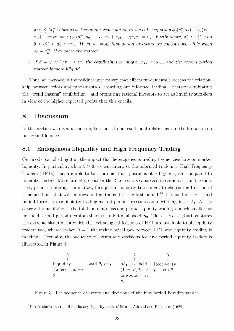
liquidity traders. More formally, consider the 2-period case analyzed in section 5.1, and assume
that, prior to entering the market, first period liquidity traders get to choose the fraction of
their positions that will be unwound at the end of the first period.19 If β = 0 in the second
period there is more liquidity trading as first period investors can unwind against −θ1. At the
other extreme, if β = 1, the total amount of second period liquidity trading is much smaller, as
first and second period investors share the additional shock u2. Thus, the case β = 0 captures
the extreme situation in which the technological features of HFT are available to all liquidity
traders too, whereas when β = 1 the technological gap between HFT and liquidity trading is
maximal. Formally, the sequence of events and decisions for first period liquidity traders is
illustrated in Figure 3.
0
Liquiditytraders chooseβ
1
Load θ1 at p1
2
βθ1 is held,(1 − β)θ1 isunwound atp2
3
Receive (v −p1) on βθ1
Figure 3: The sequence of events and decisions of the first period liquidity trader.
19This is similar to the discretionary liquidity traders’ idea in Admati and Pfleiderer (1988).
23
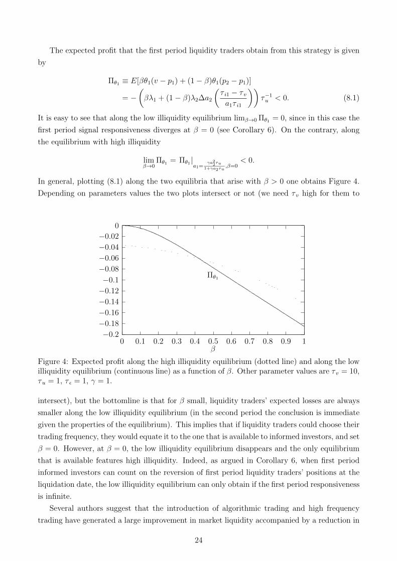
The expected profit that the first period liquidity traders obtain from this strategy is given
by
Πθ1 ≡ E[βθ1(v − p1) + (1− β)θ1(p2 − p1)]
= −(βλ1 + (1− β)λ2∆a2
(τ i1 − τ va1τ i1
))τ−1u < 0. (8.1)
It is easy to see that along the low illiquidity equilibrium limβ→0 Πθ1 = 0, since in this case the
first period signal responsiveness diverges at β = 0 (see Corollary 6). On the contrary, along
the equilibrium with high illiquidity
limβ→0
Πθ1 = Πθ1|a1=
γa22τu
1+γa2τu,β=0
< 0.
In general, plotting (8.1) along the two equilibria that arise with β > 0 one obtains Figure 4.
Depending on parameters values the two plots intersect or not (we need τ v high for them to
−0.2
−0.18
−0.16
−0.14
−0.12
−0.1
−0.08
−0.06
−0.04
−0.02
0
0 0.1 0.2 0.3 0.4 0.5 0.6 0.7 0.8 0.9 1β
Πθ1
Figure 4: Expected profit along the high illiquidity equilibrium (dotted line) and along the lowilliquidity equilibrium (continuous line) as a function of β. Other parameter values are τ v = 10,τu = 1, τ ε = 1, γ = 1.
intersect), but the bottomline is that for β small, liquidity traders’ expected losses are always
smaller along the low illiquidity equilibrium (in the second period the conclusion is immediate
given the properties of the equilibrium). This implies that if liquidity traders could choose their
trading frequency, they would equate it to the one that is available to informed investors, and set
β = 0. However, at β = 0, the low illiquidity equilibrium disappears and the only equilibrium
that is available features high illiquidity. Indeed, as argued in Corollary 6, when first period
informed investors can count on the reversion of first period liquidity traders’ positions at the
liquidation date, the low illiquidity equilibrium can only obtain if the first period responsiveness
is infinite.
Several authors suggest that the introduction of algorithmic trading and high frequency
trading have generated a large improvement in market liquidity accompanied by a reduction in
24

adverse selection risk (see, e.g. Hendershott, Jones, and Menkveld (2010)). This finding is con-
sistent with the low illiquidity equilibrium where, short of profitable speculative opportunities,
informed investors in the second period lower their exposure to the risky asset (see Proposi-
tion 3), adverse selection decreases across the two periods, and the first period price under-relies
on public information (and thus over-relies on private information, see Proposition 4).20 As
argued above, our model suggests, however, that the liquidity improvement that is brought by
HFT is not necessarily exploitable by those who are to gain the most from it, namely liquidity
traders. A further implication of our model is that with differential information, the existence of
a discrepancy in the speed at which different types of investors can turn around their positions
can be responsible for indeterminacy, making liquidity dependent on a coordination problem
across different generations of investors, and thereby endogenously creating a source of liquidity
risk.
8.2 Illiquidity and contrarian behavior
Our model predicts that investors are contrarians, acting as dealers, when the level of private
information (as measured by the difference αPn−αEn) affecting the aggregate demand is low (see
Corollary 5, and Proposition 3). In this case, indeed, as the trading process does not lead to a
considerable reduction in the uncertainty on the liquidation price, the supply of liquidity entails
high expected returns (see Corollary 8). This is what occurs in the high illiquidity equilibrium.
Conversely, in the low illiquidity equilibrium, investors step up their response to private signals,
the aggregate demand is more driven by fundamentals information, and liquidity provision is
less profitable. Based on this, we should expect that information on the supply of liquidity
represents a better proxy for price changes in the high illiquidity equilibrium, compared to
the low illiquidity equilibrium. Using (5.5), we can analyze the covariance between investors’
aggregate positions in period 1 (−θ1) and the subsequent price change (∆p2) across the two
equilibria that arise with β > 0:
Cov[−θ1,∆p2] =Vari1[p2]Var[θ1]
γ
(1 + a21
Var[εi1]
Var[θ1]
). (8.2)
The above expression captures the idea that for investors to accept clearing the market, prices
must move in a way to allow for a risk-based compensation. Several studies (see, e.g. Hen-
dershott and Seasholes (2007)) use a measure like (8.2) to document the ability of dealers’
inventory positions to forecast future returns at short horizons. While in both equilibria the
above covariance is positive, it is easy to see that for “small” values of β, Cov[−θ1,∆p2] is higher
along the equilibrium with high illiquidity. Using the result of Proposition 3, and computing
20If we measure adverse selection at time n via the OLS conditional regression coefficient of the liquidationvalue over the time n informational addition, we can verify that along the low illiquidity equilibrium adverseselection decreases between periods 1 and 2. To see this, note that along the low illiquidity equilibrium adverseselection at time 1 is a∗∗1 τu/τ1, whereas at time 2 we have (a2−βa∗∗1 )τu/τ2. As in this case ∆a2 < 0, we look atthe absolute value and check that a∗∗1 /τ1 > a∗∗1 /τ2 > |∆a2/τ2|. The first inequality is trivially always satisfied,whereas the second one requires a∗∗1 > a2/(1 + β), a condition that is always satisfied along the equilibriumwith low illiquidity.
25

the limit of (8.2) when a1 = a∗1,
limβ→0
Cov[−θ1,∆p2] =Vari1[p2]Var[θ1]
γ
(1 + a21
Var[εi1]
Var[θ1]
)∣∣∣∣a1=
γa22τu
1+γa2τu,β=0
> 0,
whereas along the low illiquidity equilibrium given that with β → 0, a∗∗1 diverges to infinity
(see Proposition 3), prices become fully revealing and Cov[−θ1,∆p2] tends to 0. Numerical
simulations confirm that this result holds also for larger values of β, as shown in Figure 5. The
0
0.1
0.2
0.3
0.4
0.5
0.6
0.7
0.8
0 0.1 0.2
Cov[−θ1,∆p2]
0.3 0.4 0.5 0.6 0.7 0.8 0.9 1
Figure 5: The figure displays the evolution of Cov[−θ1,∆p2] along the high illiquidity equi-librium (continuous line) and the low illiquidity equilibrium (dotted line) as a function of β.Parameters’ values are as follows: γ = 1, τu = τ v = τ ε = 1.
figure displays the evolution of Cov[−θ1,∆p2] along the high illiquidity equilibrium (continuous
line) and the low illiquidity equilibrium (dotted line) as a function of β. When β increases, a
lower fraction of liquidity traders revert their positions, and thus first period inventories are
a worse predictor of the next period price change along the high illiquidity equilibrium. This
explains why along the high illiquidity equilibrium Cov[−θ1,∆p2] declines with β.
The above results and Corollaries 4, 7, and 8 suggest the following interpretation for our
findings. If price risk is high, the market is illiquid, liquidity supply is thus profitable, and
informed investors act in a “market making” fashion, absorbing liquidity traders’ demand with
large price concessions (and thereby earning high expected returns from liquidity provision). If,
on the other hand, price risk is low, the market is liquid, liquidity supply is not very profitable,
and investors act as “trend chasers” (low price risk and thus low risk compensation). Whether
price risk is high or low depends on a coordination problem and we predict that high price
risk occurs when informed investors refrain from using private information exactly because
prices are mainly driven by liquidity shocks which are orthogonal to fundamentals. Conversely,
price risk is low when investors use private signals exactly because the main driver of asset
prices is fundamentals information. Therefore, liquidity provision is more profitable when there
is little informational trading in the market. Conversely, liquidity provision is less profitable
26

when the market is rife with informed trading. As argued in the introduction many authors
document the existence of a positive relationship between illiquidity and expected returns. In
our model, this effect is due to the lack of participation of rational agents in their capacity of
informed investors which prevents the reduction in fundamentals uncertainty due to order flow
and private information, thus making holding the asset more risky.
This intuition allows us to put into perspective our findings in Section 7.2. There we argued
that a shock to the residual uncertainty affecting fundamentals “crowds out” informed investors
from the market. Intuitively, a sudden increase in residual uncertainty is one of the features of
a crisis, as it implies that investors’ information is a poor guide to investment decisions based
on fundamentals. In this respect, our findings are consistent with the recent literature that
analyzes the impact of the crisis started in 2007 on investors’ behavior. Nagel (2010), shows that
expected returns from contrarian strategies for Nasdaq stocks were highly positively correlated
with the level of the VIX index during the recent crisis (2007–2009).21 Distaso, Fernandes, and
Zikes (2010), supply evidence that hedge funds of different styles reduced their exposure to the
market when the liquidity dry up climaxed. Our model provides a theoretical interpretation for
both of these facts. Indeed, our analysis shows that investors reduce their reliance on private
information, yielding a lower volume of informational trading, and act as contrarians exactly
when due to high price risk, illiquidity and the (expected) returns due to liquidity provision
are high, and the risk to face informed investors is instead low. This suggests that part of the
spike in illiquidity documented in the literature was favored by an increase in price risk due to
a lack of participation of informed investors in their capacity of liquidity suppliers.
8.3 Relationship to behavioral finance
Our results also provide an alternative interpretation for several findings in the literature on
behavioral finance.
Barber and Odean (2000), analyzing the trading activity of investors at discount brokerage
firms in the period 1991–1996, find that taking into account trading costs, the average returns
of their portfolios are consistently below those of standard benchmarks. Their conclusion is that
investors are overconfident and tend to trade even in the absence of relevant information. Our
results can accommodate these findings. In the low illiquidity equilibrium investors overreact
to their information (compared to the static solution). 22 This is because they anticipate that
at the interim liquidation date they face lower adverse selection and thus lower illiquidity, so
that their signals allow a better prediction of the liquidation price. Overreaction to private
information has two implications: (1) it heightens information impounding, lowering price risk
and reducing expected returns (Corollary 8) and (2) it yields higher volume of informational
trading (Corollary 7). Taken together the above two points provide an alternative explanation
for the pattern of poor return performance and “excessive” trading which does not rely on the
existence of behavioral biases.
21The VIX is traditionally interpreted as a measure of financial intermediaries’ risk-appetite (this is, e.g., theinterpretation in Adrian and Shin (2010)).
22Indeed, the static solution calls for a1 = γτ ε, and it is easy to check that 0 < a∗1 < γτ ε < a∗∗1 .
27

Our results are also related to the literature on noise traders’ risk (De Long et al. (1990)).
In our setup, the inability to pin down the illiquidity of the market at which short term in-
vestors unwind their position, creates liquidity risk. This can prevent investors from acting
aggressively on their information, making prices poor indicators of the underlying liquidation
value (Proposition 3). Therefore, our paper shows that liquidity risk can play a role similar to
that of noise traders’ risk in hindering the action of informed investors, and eventually making
prices worse estimators of fundamentals.
9 Conclusions
When a market is populated by short term investors, the persistence of liquidity traders’ demand
implies that only a fraction of the latters’ orders is bound to revert when informed investors
close out their positions. Hence, each cohort of investors unwinds part of its holdings against
the aggregate demand coming from the next period cohort, thereby shifting part of the risk
it incorporates and potentially facing an adverse selection problem at the liquidation date.
This makes portfolio decisions more sensitive to the illiquidity of the market in which investors
plan to unwind their positions. With heterogeneous information, a more illiquid market in the
future, lowers price dependence on fundamentals, reducing investors’ reliance on their private
information. Conversely, when investors anticipate a more liquid future market they over-rely
on their private signals. Thus, with persistent liquidity trades and heterogeneous infomation,
short term horizons deliver multiple equilibria which can be ranked in terms of illiquidity.
We show that along the equilibria in which investors anticipate higher future illiquidity,
prices are driven by HOEs about fundamentals, and therefore over-rely on public information.
In these equilibria investors scale down their response to private signals yielding an increase in
price risk, which implies that returns from liquidity provision are higher. Indeed, it is precisely
in these equilibria that contrarian strategies are profitable, as the aggregate demand for the
stock features little private information. When instead investors anticipate a more liquid market
in the future, they step up their response to private signals, reducing price risk and returns from
liquidity provision. In this case, indeed, investors are trend chasers as the aggregate demand
for the stock is rife with private information.
Our model sheds light on the implications that heterogeneous trading frequencies have for
market illiquidity. Indeed, while along the low illiquidity equilibrium, liquidity traders’ losses
are minimized, this equilibrium disappears whenever trading frequencies coincide. Thus, an
implication of our analysis is that while trading at high frequencies may generate liquidity im-
provements, these improvements are not necessarily exploitable by those who are to gain the
most from it, namely liquidity traders. A further implication of our model is that with differen-
tial information, heterogenous trading frequencies make liquidity dependent on a coordination
problem across different generations of investors, and thereby can endogenously create liquidity
risk.
Our model also provides a theoretical foundation to the empirical regularity that links
illiquidity to expected returns. In our story, a more illiquid market is one in which price risk
28

is huge exactly because the response to private information is subdued, and investors require
a higher compensation (price concession) to hold the inventory of the risky asset. Based on
this intuition we show that a spike in the residual uncertainty that affects fundamentals causes
the impact of private information on the aggregate demand to wane, singling out as a unique
equilibrium the one in which investors are contrarians.
Finally, our paper is related to several findings of the behavioral finance literature. As
we argued, our results can capture overreliance on private information without requiring that
investors suffer from overconfidence, thereby implying that patterns of high informational vol-
ume and low expected returns can be generated within a model in which, except for liquidity
traders, all investors are rational. Furthermore, as explained, liquidity risk (as opposed to noise
traders’ risk) can act as a powerful deterrent to the action of short-term, informed investors,
leading prices to reflect poorly the impact of fundamentals information.
Our paper raises a number of potentially interesting issues. First, as pointed out in sec-
tion 8.3, in our context short term investors’ inability to effectively coordinate on one equilib-
rium creates liquidity risk, which similarly to behavioral finance noise traders’ risk, is responsible
for investors’ lack of action on their information and poor price informativeness. This raises
the issue of limits to arbitrage.23 Also, as argued in section 8.1, with short-term investors
persistence in liquidity trades can be seen as a reduced form for the existence of differential
trading frequencies across investors’ classes. This raises the issue of the welfare impact of High
Frequency Trading. We leave these and other issues to future research.
23For instance, short term trading can distract prices from the benchmark they achieve when all investorshave a long term horizon (Cespa and Vives (2009)).
29

References
Acharya, V. V. and L. H. Pedersen (2005). Asset pricing with liquidity risk. Journal of
Financial Economics 77 (2), 375–410.
Admati, A. R. and P. Pfleiderer (1988). A theory of intraday patterns: volume and price
variability. Review of Financial Studies 1 (1), 3–40.
Adrian, T. and H. S. Shin (2010). Liquidity and leverage. Journal of Financial Intermedia-
tion 19 (3), 418–437.
Allen, F., S. Morris, and H. S. Shin (2006). Beauty contests and iterated expectations in
asset markets. Review of Financial Studies 19 (3), 719–752.
Amihud, Y. and H. Mendelson (1986). Asset pricing and the bid-ask spread. Journal of
Financial Economics 17 (2), 223–249.
Bacchetta, P. and E. van Wincoop (2008). Higher order expectations in asset pricing. Journal
of Money, Credit and Banking 40 (5), 837–866.
Banerjee, S., R. Kaniel, and I. Kremer (2009). Price drift as an outcome of differences in
higher order beliefs. Review of Financial Studies 22 (9), 3707–3734.
Barber, B. M. and T. Odean (2000). Trading is hazardous to your wealth: the common stock
performance of individual investors. Journal of Finance 55, 773–806.
Barberis, N. and R. Thaler (2003). A survey of behavioral finance, Chapter 18, pp. 1051–1121.
Handbook of the Economics of Finance. Elsevier Science B.V.
Biais, B. and P. Bossaerts (1998). Asset prices and trading volume in a beauty contest.
Review of Economic Studies 65 (2), 307–340.
Boehmer, E. and J. Wu (2006). Order flow and prices. Working Paper .
Brennan, M. J. and A. Subrahmanyam (1996). Market microstructure and asset pricing: On
the compensation for illiquidity in stock returns. Journal of Financial Economics 41 (3),
441–464.
Cao, H. H. and H. Ou-Yang (2005). Bubbles and panics in a frictionless market with hetero-
geneous expectations. Working Paper .
Cespa, G. (2002). Short-term investment and equilibrium multiplicity. European Economic
Review 46 (9), 1645–1670.
Cespa, G. and X. Vives (2009). Dynamic trading and asset prices: Keynes vs. Hayek. CEPR
Discussion Paper n. 7506 .
Comerton-Forde, C., T. Hendershott, C. M. Jones, P. C. Moulton, and M. S. Seasholes
(2010). Time variation in liquidity: The role of market-maker inventories and revenues.
Journal of Finance 65 (1), 295–331.
De Long, J. B., A. Shleifer, L. H. Summers, and R. J. Waldmann (1990). Noise trader risk
in financial markets. Journal of Political Economy 98 (4), 703–738.
30

Distaso, W., M. Fernandes, and F. Zikes (2010). Tailing tail risk in the hedge fund industry.
Working Paper, Queen Mary Univerity of London and Imperial College Business School .
Dow, J. and G. Gorton (1994). Arbitrage chains. Journal of Finance 49 (3), 819–49.
Easley, D., R. F. Engle, M. O’Hara, and L. Wu (2008). Time-varying arrival rates of informed
and uninformed trades. Journal of Financial Econometrics 6 (2), 171–207.
Froot, K. A., D. S. Scharfstein, and J. C. Stein (1992). Herd on the street: Informational
inefficiencies in a market with short-term speculation. Journal of Finance 47 (4), 1461–
1484.
Grossman, S. J. and M. H. Miller (1988). Liquidity and market structure. Journal of Fi-
nance 43 (3), 617–37.
He, H. and J. Wang (1995). Differential information and dynamic behavior of stock trading
volume. Review of Financial Studies 8 (4), 919–972.
Hendershott, T., C. M. Jones, and A. Menkveld (2010). Does algorithmic trading improve
liquidity? Journal of Finance 66 (1), 1–33.
Hendershott, T. and M. S. Seasholes (2007). Market maker inventories and stock prices. The
American Economic Review 97 (2), 210–214.
Kandel, E. and N. D. Pearson (1995). Differential interpretation of public signals and trade
in speculative markets. Journal of Political Economy 103 (4), 831–872.
Kondor, P. (2009). The more we know, the less we agree: higher-order expectations, public
announcements and rational inattention. Working Paper .
Morris, S. and H. S. Shin (2002). The social value of public information. American Economic
Review 92, 1521–1534.
Nagel, S. (2010). Evaporating liquidity. MIMEO Stanford University .
Nimark, K. P. (2007). Dynamic higher order expectations. Working Paper .
Ottaviani, M. and P. N. Sørensen (2009). Aggregation of information and beliefs: asset
pricing lessons from prediction markets. Working Paper .
Pastor, L. and R. F. Stambaugh (2003). Liquidity risk and expected stock retums. The
Journal of Political Economy 111 (3), pp. 642–685.
Saar, G. and J. Linnainmaa (2010). Lack of anonimity and the inference from order flow.
Working Paper .
Singleton, K. J. (1987). Asset prices in a time-series model with disparately informed, com-
petitive traders. In W. Barnett and K. Singleton (Eds.), New approaches to monetary
economics. Cambridge University Press, Cambridge.
Vayanos, D. (1998). Transaction costs and asset prices: A dynamic equilibrium model. Review
of Financial Studies 11 (1), 1–58.
31

Vives, X. (1995). Short-term investment and the informational efficiency of the market.
Review of Financial Studies 8 (1), 125–160.
Vives, X. (2008). Information and Learning in Markets: The Impact of Market Microstruc-
ture. Princeton University Press.
32

A Appendix
Proof of Proposition 1
Assume that in a linear equilibrium xn = −φn(pn), with φn(·) a linear function of pn. This
implies that the market clearing equation at time n reads as follows:
xn + θn = 0⇔ −φn(pn) + θn = 0.
Hence, at equilibrium pn is observationally equivalent to θn, i.e. at time n rational investors
know the realisation of the noise shock θn. To solve for the equilibrium we proceed by backward
induction and start from the third trading round, where due to CARA and normality, we have
X3(p3) = γE3[v]− p3
Var3[v](A.1)
= −Λ−13 (p3 − v),
with
Λ3 ≡1
γτ v, (A.2)
and
p3 = v + Λ3θ3. (A.3)
In the second period, we have
X2(p2) = γE2[p3]− p2
Var2[p3](A.4)
= −Λ−12 (p2 − v),
with
Λ2 ≡1 + γβΛ−13 τu
γΛ−23 τu, (A.5)
and
p2 = v + Λ2θ2. (A.6)
Similar calculations show that in the first period x1 = −Λ−11 (p1 − v) and p1 = v + Λ1θ1, with
Λ1 ≡1 + γβΛ−12 τu
γΛ−22 τu.
QED
Proof of Corollary 1
In the third period Λ3 = 1/γτ v, implying that ∂Λ3/∂β = 0. In the second period, us-
ing (A.5), ∂Λ2/∂β = Λ3 > 0. Finally, in the first period we have
Λ1 =Λ2
2
γτu+ βΛ2,
which is increasing in β. QED
The following lemma establishes that working with the sequence zn ≡ {zt}nt=1 is equivalent
to working with pn ≡ {pt}nt=1:
33

Lemma 3. In any linear equilibrium the sequence of informational additions zn is observation-
ally equivalent to pn.
Proof. Consider a candidate equilibrium in linear strategies xin = ansin − ϕn(pn). In the first
period imposing market clearing yields∫ 1
0a1si1 − ϕ1(p1)di + θ1 = a1v − ϕ1(p1) + θ1 = 0 or,
denoting with z1 = a1v+θ1 the informational content of the first period order-flow, z1 = ϕ1(p1),
where ϕ1(·) is a linear function. Hence, z1 and p1 are observationally equivalent. Suppose now
that zn−1 = {z1, z2, . . . , zn−1} and pn−1 = {p1, p2, . . . , pn−1} are observationally equivalent and
consider the n-th period market clearing condition:∫ 1
0Xn(sin, p
n−1, pn)di + θn = 0. Adding
and subtracting∑n−1
t=1 βn−t+1atv, the latter condition can be rewritten as follows:
n∑t=1
zt − ϕn(pn) = 0,
where ϕn(·) is a linear function, zt = ∆atv + ut denotes the informational content of the t-th
period order-flow, and ∆at = at − βat−1,. As by assumption pn−1 and zn−1 are observationally
equivalent, it follows that observing pn is equivalent to observing zn. 2
Proof of Proposition 2
We provide this proof assuming that residual uncertainty affects the final liquidation value
(τ δ <∞). As the reader can easily verify our argument goes through also when we set τ δ →∞.
To prove our argument, we proceed by backwards induction. In the last trading period traders
act as in a static model and owing to CARA and normality we have
X3(si3, z3) = γ
Ei3[v]− p3Vari3[v + δ]
, (A.7)
and
p3 = αP3
(v +
θ3a3
)+ (1− αP3)E3[v], (A.8)
where
a3 =γτ ε
1 + κ, (A.9)
αP3 =τ ετ i3
, (A.10)
κ = τ−1δ τ i3. An alternative way of writing the third period equilibrium price is
p3 = λ3z3 + (1− λ3∆a3)p2, (A.11)
where
λ3 = αP3
1
a3+ (1− αP3)
∆a3τuτ 3
, (A.12)
34

captures the price impact of the net informational addition contained in the 3rd period aggregate
demand, while
p2 =αP3τ 3β(
∑2t=1 β
2−tzt) + (1− αP3)a3τ 2E2[v]
αP3τ 3βa2 + (1− αP3)a3τ 2
=γτ 2E2[v] + β(1 + κ)(z2 + βz1)
γτ 2 + βa2(1 + κ), (A.13)
zn = ∆anv + un, and ∆an = an − βan−1.
Second Period
In the second period owing to CARA and normality, an agent i trades according to
X2(si2, z2) =
γ(Ei2[p3]− p2)Vari2[p3]
, (A.14)
where
Ei2[p3] = λ3∆a3Ei2[v] + (1− λ3∆a3)p2. (A.15)
Vari2[p3] = λ23
(τ i3τ i2τu
). (A.16)
Replacing (A.15) and (A.16) in (A.14) yields
X2(si2, z2) =
γ∆a3τ i2τuλ3τ i3
(Ei2[v]− p2) +γτ i2τu
λ23τ i3(p2 − p2).
Imposing market clearing and identifying equilibrium parameters yields
p2 = αP2
(v +
θ2a2
)+ (1− αP2)E2[v], (A.17)
where
αP2 ≡ αE2
(1 +
(βρ2 − 1)τ 2τ i3
)(A.18)
a2 =γ∆a3τuτ ελ3τ i3
, (A.19)
and ρ2 ≡ a2(1 + κ)/(γ∑2
t=1 τ εt). Alternatively, in the spirit of what done for the third period
analysis
p2 = λ2z2 + (1− λ2∆a2)p1, (A.20)
where
λ2 = αP2
1
a2+ (1− αP2)
∆a2τuτ 2
, (A.21)
and
p1 =αP2τ 2βz1 + (1− αP2)a2τ 1E1[v]
αP2τ 2βa1 + (1− αP2)a2τ 1. (A.22)
Finally, note that using (A.18) and (A.19) and rearranging the expression for the second period
strategy yields
X2(si2, z2) =
a2αE2
(Ei2[v]− p2) +αP2 − αE2
αE2
a2αP2
(p2 − E2[v]).
35

First period
To compute the first period equilibrium we can use the results of the second period analysis.
Indeed, X1(si1, z1) = (γ/Vari1[p2])(Ei1[p2]− p1) and using (A.20)
Ei1[p2] = λ2∆a2Ei1[v] + (1− λ2∆a2)p1
Vari1[p2] = λ22
(τ i2τ i1τu
),
The above expressions highlight the recursive structure of the problem and imply
X1(si1, z1) =γ∆a2τ i1τuλ2τ i2
(Ei1[v]− p1) +γτ i1τu
λ22τ i2(p1 − p1),
and
p1 = αP1
(v +
θ1a1
)+ (1− αP1)E1[v], (A.23)
where
αP1 = αE1
(1 + τ 1
(γαP2(βρ1 − ρ2)
a2+
(βρ2 − 1)
τ i3
)), (A.24)
a1 =γ∆a2τuτ ελ2τ i2
, (A.25)
and ρ1 ≡ a1(1 + κ)/(γτ ε1). In the first period too we can express the price as
p1 = λ1z1 + (1− λ1a1)v,
with
λ1 = αP1
1
a1+ (1− αP1)
a1τuτ 1
,
and, using (A.24), obtain that
X1(si1, z1) =a1αE1
(Ei1[v]− p1) +αP1 − αE1
αE1
a1αP1
(p1 − E1[v]). (A.26)
QED
Proof of Corollary 2
The first part of the Corollary is proved in the paper. For the second part, we show how
to obtain the expression for Λ2, the argument for Λ1 being similar. Imposing market clearing
on (A.7) yields
p3 = E3[v] +Vari3[v + δ]
γθ3,
where E3[v] ≡∫ 1
0Ei3[v]di. Similarly, due to short term horizons, the second period price is
given by
p2 = E2[p3] +Vari2[p3]
γθ2
= E2
[E3[v]
]+
Vari3[v + δ]
γβE2 [θ2] +
Vari2[p3]
γθ2
= αP2v + (1− αP2)E2[v] +
(β
Vari3[v + δ]
γ+
Vari2[p3]
γ
)θ2, (A.27)
36
where
αP2 = αE2 +Vari3[v + δ]
γβa2(1− αE2),
and αE2 is given by:
αE2 = αE2
(1− τ 2
τ 3(1− αE3)
).
Now, we know that at a linear equilibrium
p2 = αP2
(v +
θ2a2
)+ (1− αP2)E2[v]. (A.28)
Comparing (6.3) and (A.28), we then see that an alternative expression for a2 is the following:
a2 = γαP2
Vari2[p3] + βVari3[v + δ].
Given that we define the reciprocal of market depth in period 2 as Λ2 ≡ αP2/a2, from the last
equation we can conclude that
Λ2 =Vari2[p3] + βVari3[v + δ]
γ. (A.29)
QED
Proof of Corollary 3
To obtain equation (5.5) we start from the equilibrium price equation at time n:
pn = αPn
(v +
θnan
)+ (1− αPn)En[v],
and expanding the expression for θn, we obtain
pn =αPnan
(anv + un + βθn−1) + (1− αPn)En[v].
Adding and subtracting (αPn/an)βan−1v at the r.h.s. of the above expression and rearranging
pn = λnzn +βαPnan
(an−1v + θn−1) + (1− αPn)τn−1τn
En−1[v], (A.30)
where zn ≡ ∆anv + un = (an − βan−1)v + un, and
λn = αPn1
an+ (1− αPn)
∆anτuτn
.
Adding and subtracting (1− λn∆an)pn−1 to the r.h.s. of (A.30) yields
pn = λnzn + (1− λn∆an)pn−1 − (1− λn∆an)×(αPn−1
an−1(an−1v + θn−1) + (1− αPn−1)En−1[v]
)+βαPnan
(an−1v + θn−1) + (1− αPn)τn−1τn
En−1[v]
= λnzn + (1− λn∆an) pn−1 +
(βαPnan− (1− λn∆an)
αPn−1
an−1
)En−1[θn−1]. (A.31)
37

We now prove that
βαPnan− (1− λn∆an)
αPn−1
an−1= λn∆an
αPn−1 − αEn−1
an−1.
Starting from the third period price we have
p3 = αP3
(v +
θ3a3
)+ (1− αP3)E3[v] (A.32)
= λ3z3 + (1− λ3∆a3) p2 +
(βαP3
a3− (1− λ3∆a3)
αP2
a2
)E2[θ2].
Now using the definition for αP3 we obtain
βαP3
a3− (1− λ3∆a3)
αP2
a2=β(1 + κ)
γτ i3− γτ 2 + β(1 + κ)a2
γτ i3
αP2
a2
=β(1 + κ)a2 + γτ 2
γτ i3
(β(1 + κ)
β(1 + κ)a2 + γτ 2− αP2
a2
)=
(1 + κ)(β(1 + κ)a2 + γτ 2)
γτ i3
(β
β(1 + κ)a2 + γτ 2− 1
γρ2τ i2
(1 +
(βρ2 − 1)τ 2τ i3
))=
1 + κ
γ2ρ2τ i2τ i3
(γτ 1(βρ2 − 1)− (β(1 + κ)a2 + γτ 2)
(βρ2 − 1)τ 2τ i3
)=
(1 + κ)(βρ2 − 1)τ 2γ2ρ2τ i2τ
2i3
(γτ i3 − β(1 + κ)a2 − γτ 2)
=(1 + κ)(βρ2 − 1)τ 2
γρ2τ i2τ i3λ3∆a3
= λ3∆a3αP2 − αE2
a2,
where we use the definition of αP2 to move from the second to the third row of the above
expression. Summarizing, using the above result the second period price can be expressed as
follows:
p3 = λ3z3 + (1− λ3∆a3) p2 + λ3∆a3αP2 − αE2
a2E2[θ2]. (A.33)
Going back one period, we need to prove that
βαP2
a2− (1− λ2∆a2)
αP1
a1= λ2∆a2
αP1 − αE1
a1. (A.34)
To prove this, we start by noting that
βαP2
a2− (1− λ2∆a2)
αP1
a1=
1
a1
(αP1λ2∆a2 +
βαP2
a2a1 − αP1
),
which in turn implies that (A.34) is correct if and only if
αP1 = αE1λ2∆a2 +βαP2
a2a1. (A.35)
38

To prove that the above expression is correct, we manipulate the definition of αP1 to obtain:
αP1 = αE1
(1 +
γτ 11 + κ
(αP2(βρ2 − ρ1)
a2+αP3(βρ2 − 1)
a3
))= αE1
(1 + τ 1
(αP2
a2
(βa1τ ε1− a2∑2
t=1 τ εt
)+βρ2 − 1
τ i3
))
=αP2
a2βa1 + αE1
(1− αP2
a2βa1 +
(βρ1 − 1
τ i3− αP2∑2
t=1 τ εt
)). (A.36)
Thus, to prove our claim we need to show that
1− αP2
a2βa1 +
(βρ1 − 1
τ i3− αP2∑2
t=1 τ εt
)= λ2∆a2. (A.37)
According to our definition of αP2 we have
αP2 = αE2
(1 +
(βρ2 − 1)τ 2τ i3
),
which in turn implies that
1− αP2 = (1− αE2)
(1−
∑2t=1 τ εtτ i3
(βρ2 − 1)
). (A.38)
Rearranging (A.37) yields
1− αP2
a2βa1 +
(βρ1 − 1
τ i3− αP2∑2
t=1 τ εt
)=αP2
a2∆a2 + (1− αP2)−
τ 1∑2t=1 τ εt
(αP2 −
∑2t=1 τ εt(βρ2 − 1)
τ i3
)=αP2
a2∆a2 + (1− αP2)−
τ 1τ 2
(1− αP2)
= λ2∆a2, (A.39)
where we use (A.38) to simplify the first row of the above expression. This allows us to write
p2 = λ2z2 + (1− λ2∆a2)p1 + λ2∆a2αP1 − αE1
a1E1[θ1], (A.40)
and completes our proof. QED
Proof of Proposition 4
Rearranging (5.5) yields
pn+1 − pn = λn+1
(zn+1 + ∆an+1
αPn − αEnan
En[θn]−∆an+1pn
)= λn+1∆an+1
((1− αEn)(v − En[v])− αEn
anθn
)+ λn+1un+1,
and recalling that
an = γλn+1∆an+1αEn
Varin[pn+1],
39

we can see that from the point of view of period n investors
En[pn+1 − pn] = −λn+1∆an+1αEnan
En[θn]
= −Varin[pn+1]
γEn[θn]. (A.41)
QED
Proof of Corollary 5
The expression for rational investors’ strategies are obtained in the proof of Proposition 2,
whereas those for αP2 and αP1 follow immediately after rearranging (A.18) and (A.24). The
recursive equation defining the couple a1, a2 follows from (A.19) and (A.25).
QED
Proof of Proposition 3
For any β ∈ [0, 1], in the second period an equilibrium must satisfy a2 = γτ ε. In the first
period an equilibrium must satisfy
φ1(a1, a2) ≡ a1λ2(τ 2 + τ ε)− γτ ε∆a2τu= a1(1 + γτu∆a2)− γ2τ ε∆a2τu = 0. (A.42)
The above equation is a quadratic in a1 which for any a2 > 0 and β > 0 possesses two positive,
real solutions:
a∗1 =1 + γτu(a2 + βγτ ε)−
√1 + γτu(2(a2 + βγτ ε) + γτu(a2 − βγτ ε)2)
2βγτu(A.43)
a∗∗1 =1 + γτu(a2 + βγτ ε) +
√1 + γτu(2(a2 + βγτ ε) + γτu(a2 − βγτ ε)2)
2βγτu, (A.44)
with a∗∗1 > a∗1. This proves that for β > 0 there are two linear equilibria.
Inspection of the above expressions for a1 shows that βa∗1 < a2, while βa∗∗1 > a2. This implies
that βρ1 > 1 for a1 = a∗∗1 and βρ1 < 1 otherwise. Thus, using (5.9), we obtain αP1(a∗1, a2) <
αE1(a∗1, a2), and αP1(a
∗∗1 , a2) > αE1(a
∗∗1 , a2). The result for second period illiquidity follows from
substituting (A.43) and (A.44) in λ2. To see that prices are more informative along the low
illiquidity equilibrium note that in the first period Var[v|z1]−1 = τ 1 = τ v + a21τu. In the second
period, the price along the low illiquidity equilibrium is more informative than along the high
illiquidity equilibrium if and only if
(1 + β2 + γa2τu((1− β2) + β(1 + β2)))√
(1 + γa2τu(1 + β))2 − 4β(γa2τu)2
γ2β2τu> 0,
which is always true.
40

To see that with β = 0, a unique equilibrium arises, note that
limβ→0
1 + γτu(a2 + βγτ ε) +√
1 + γτu(2(a2 + βγτ ε) + γτu(a2 − βγτ ε)2)2βγτu
=∞,
while, using l’Hospital’s rule,
limβ→0
1 + γτu(a2 + βγτ ε)−√
1 + γτu(2(a2 + βγτ ε) + γτu(a2 − βγτ ε)2)2βγτu
=γa22τu
1 + γa2τu.
From (5.9) it then follows that in this case αP1 < αE1 . Finally, taking the limit of λ2 as β → 0
when a1 = a∗1 yields
limβ→0
λ2(a∗1, a2) =
1 + γτua2γ(τ v + (a∗1)
2τu + a22τu + τ ε)> 0,
whereas limβ→0 λ2(a∗∗1 , a2) = 0. QED
Proof of Lemma 2
Note that at any linear equilibrium En[θn] = an(v−En[v]) + θn. This, in turn, allows us to
express the equilibrium price as follows:
pn = En[v] +αPn − αEn
anEn[θn] +
αEnan
θn.
As a consequence
pn − v = En[v]− v +αPn − αEn
anEn[θn] +
αEnan
θn.
Thus, if αPn > αEn the price is closer to the fundamentals compared the consensus opinion,
while the opposite occurs whenever αPn < αEn .
We now prove that at equilibrium (6.11) and (6.12) are equivalent. To see this, note that
using (5.1) the covariance between pn and v is given by
Cov[v, pn] = αPn1
τ v+ (1− αPn)
(1
τ v− 1
τn
), (A.45)
and carrying out a similar computation for the time n consensus opinion
Cov[En[v], v
]= αEn
1
τ v+ (1− αEn)
(1
τ v− 1
τn
), (A.46)
where τn ≡ Var[v|pn] = τ v +τu∑n
t=1 ∆a2t . We can now subtract (A.46) from (A.45) and obtain
Cov[pn − En[v], v
]=αPn − αEn
τn, (A.47)
implying that the price at time n over relies on public information if and only if the covariance
between the price and the fundamentals falls short of that between the consensus opinion and
the fundamentals. QED
41

Proof of Corollary 9
For any 1/τ δ > 0, β ∈ [0, 1], in the second period an equilibrium must satisfy a2 = (1 +
κ)−1γτ ε. Rearranging the latter condition we obtain the following cubic in a2:
φ2(a1, a2) ≡ a32τu − 2a22a1βτu + a2(τ 1 + τ δ + (βa1)
2 τu + τ ε)− γτ δτ ε = 0. (A.48)
Differentiating (A.48) with respect to a2 yields
∂φ2(a1, a2)
∂a2= 3a22τu − 4a2a1βτu + τ 1 + τ δ + (βa1)
2 τu + τ ε,
a quadratic whose discriminant is given by
∇ = 4τu(a21τu(β
2 − 1)− 3τu (τ v + τ δ + τ ε)− 2a21τu),
which is always negative for all β < 1. This implies that for any a1,
∂φ2(a1, a2)
∂a2> 0, (A.49)
and thus that for any a1, there always exists a unique real solution a∗2 ∈ (0, γτ ε) to (A.48) which
defines the second period equilibrium signal responsiveness. In the first period an equilibrium
must satisfy
φ1(a1, a2) ≡ a1λ2(τ 2 + τ ε)− γτ ε∆a2τu= a1(1 + γτu∆a2)− γ2τ ε∆a2τu = 0. (A.50)
The above equation is a quadratic in a1 which for any a2 > 0 and β > 0 possesses two positive,
real solutions:
a∗1 =1 + γτu(a2 + βγτ ε)−
√1 + γτu(2(a2 + βγτ ε) + γτu(a2 − βγτ ε)2)
2βγτu(A.51)
a∗∗1 =1 + γτu(a2 + βγτ ε) +
√1 + γτu(2(a2 + βγτ ε) + γτu(a2 − βγτ ε)2)
2βγτu, (A.52)
with a∗∗1 > a∗1. This proves that for β > 0 there are two linear equilibria.
From implicit differentiation we have
∂a2∂a1
=∂φ2(a1, a2)/∂a2
∆a2.
According to (A.49), the numerator in the above expression is positive, and since using (A.51)
and (A.52) a∗2−βa∗1 > 0, while a∗∗2 −βa∗∗1 < 0, we can conclude that a∗∗2 < a∗2. As argued above
βa∗1 < a∗2, while βa∗∗1 > a∗∗2 . This implies that βρ1 > 1 for a1 = a∗∗1 and βρ1 < 1 otherwise.
Thus, using (5.9), we obtain αP1(a∗1, a∗2) < αE1(a
∗1, a∗2), and αP1(a
∗∗1 , a
∗∗2 ) > αE1(a
∗∗1 , a
∗∗2 ).
The result for second period illiquidity follows immediately from the fact that Λ2 = Vari2[v+
δ]/γ = (τ−1i2 + τ−1δ )/γ, where τ i2 = τ v + τu(a21 + (∆a2)
2) + τ ε.
42

To see that with β = 0, a unique equilibrium arises, note that
limβ→0
1 + γτu(a2 + βγτ ε) +√
1 + γτu(2(a2 + βγτ ε) + γτu(a2 − βγτ ε)2)2βγτu
=∞,
while, given that a2 < γτ ε, and using l’Hospital’s rule
limβ→0
1 + γτu(a2 + βγτ ε)−√
1 + γτu(2(a2 + βγτ ε) + γτu(a2 − βγτ ε)2)2βγτu
=γa22τu
1 + γa2τu.
From (5.9) it then follows that in this case αP1 < αE1 .
We now check what happens to ρ1 = a1(τ δ + τ 2 + τ ε)/(γτ δτ ε) as τ δ → 0. Notice that
limτδ→0
a1 = limτδ→0
γ2τ δτ ετu∆a2 (τ 2 + τ ε)
(τ 2 + τ ε) (τ δ(1 + γ∆a2τu) + (τ 2 + τ ε))= 0,
and limτδ→0 a2 = limτδ→0 γτ δτ ε/(τ δ + (τ 2 + τ ε)) = 0. Then,
limτδ→0
ρ1 = limτδ→0
γτu∆a2 (τ 2 + τ ε)
τ 2 + τ ε= 0,
since, as argued above, in the limit a1 = a2 = 0. By continuity of ρ1 as a function of (a1, a2),
there must then exist an interval (0, τ ∗δ), such that for all τ δ ∈ (0, τ ∗δ) we have ρ1 < 1. As an → 0,
second period illiquidity coincides with the one of the market without private information, and
since Var[v + δ|si2, p2] ≤ Var[v + δ], the result follows. QED
43