higher-order finite-difference methods for partial ... · pending upon characteristic directions a...
TRANSCRIPT

Higher-Order Finite-Difference Methods for
Partial Differential Equations
by Tasleem Akhter Cheema
Department of Mathematics and Statistics,
BruneI University,
Uxbridge, Middlesex, England. UB8 3PH
A thesis submitted for the degree of
Doctor of Philosophy
September 1997

To my parents and my children
Shozab Ali, Tansheet Ali and Aisha Tasneem.
Abstract
This thesis develops two families of numerical methods, based upon rational
approximations having distinct real poles, for solving first- and second-order
parabolic/ hyperbolic partial differential equations. These methods are third
and fourth-order accurate in space and time, and do not require the use of
complex arithmetic. In these methods first- and second-order spatial deriv
atives are approximated by finite-difference approximations which produce
systems of ordinary differential equations expressible in vector-matrix forms.
Solutions of these systems satisfy recurrence relations which lead to the devel
opment of parallel algorithms suitable for computer architectures consisting
of three or four processors. Finally, the methods are tested on advection,
advection-diffusion and wave equations with constant coefficients.
11

ACKNOWLEDGEMENTS
I am pleased to express my warmest thanks to my supervisor Professor E. H.
Twizell for his invaluable suggestions, continuous encouragement and con
structive criticism during both the period of research and the writing of this
thesis. He has always given patiently of his time and tolerated my untimely
disturbance.
I also express my sincere gratitude to Dr. S.A . Matar for his continuous
guidance in using the computer packages La1EX and MATLAB.
I would like to thank the Government of Pakistan for granting ex-Pakistan
leave during the period of study.
I am indebted to my husband for his moral and financial support.
III

Contents
1 Preliminaries
1.1 Introduction.
1.2 Method of Lines.
1.3 Rational Approximations to exp(t)
1.4 Notations ........... .
1.5 Analysis of Difference Schemes .
1.5.1
1.5.2
1.5.3
1.5.4
1.5.5
Local Truncation Error .
Local Discretization Error
Consistency
Stability ..
Convergence .
. . . . . . . . . . . . . . . . .
2 Third-Order Numerical Methods for the Advection Equa-
1
1
3
3
4
5
5
5
5
6
8
tion 10
IV

2.1 Introduction............................ 10
2.2 The Model Problem. . . . . . . . . . . . . . . . . . . . . . .. 11
2.3 The Method. . . . . . . . . . . . . . . . . . . . . . . . . . .. 11
2.4 Algorithm .. ....................... 20
2.5 Numerical Examples . . . . . . . . . . . . . . . . . . . . . .. 22
2.5.1 Example 1 . . . . . . . . . . . . . . . . . . . . . . . .. 23
2.5.2 Example 2. ....................... 24
2.6 Non-linear Problem . . . . . . . . . . . . . . . . . . . . . . . . 2.5
3 Fourth-Order Numerical Methods for the Advection Equa-
tion 42
3.1 The Method . · ................... 42
3.2 Algorithm .. · . . . . . . . . . . . . . . . . . . . 58
3.3 Numerical Examples · ................... 62
3.3.1 Example 1 . · ................... 62
3.3.2 Example 2 . . . . . . . . . . . . . . . . . . . . . . . . . 63
4 Third-Order Methods for the Advection-Diffusion Equation 71
4.1 The Model Problem. . . . . . . . . . . . . . . . . . . . . . .. 71
4.2 The Method. . . . . . . . . . . . . . . . . . . . . . . . . . .. 72
v

4.3 Algorithm . . . . . . . . . . . . . . . . . . . . . . . . . . . .. 77
4.4 Numerical Example. . . . . . . . . . . . . . . . . . . . . . .. 79
5 Fourth-Order Numerical Methods for the Advection-Diffusion
Equation 85
5.1 The Method. . . . . . . . . . . . . . . . . . . . . . . . . . . . 85
5.2 Algorithm .. . ...................... 93
5.3 Numerical Example. . . . . . . . . . . . . . . . . . . . . . .. 96
6 Third-Order Finite-Difference Methods for Second-Order Hy-
perbolic Partial Differential Equations 102
6.1 The Model Problem. . . · 102
6.2 Discretization of R U oR · 103
6.3 The Method . . . . . . . · 103
6.4 Solution at the First Time-Step · 106
6.5 Rational Approximation to Matrix Exponential Function . 107
6.6
6.7
6.8
Accuracy .............. .
Development of Parallel Algorithm
Numerical Examples
6.8.1
6.8.2
Example 1 .
Example 2 .
VI
· 108
· 110
· 111
111
113

7 Fourth-Order Finite-Difference Methods for Second-Order
Hyperbolic Partial Differential Equations 120
7.1 The method . . . . . . . . . . . · 120
7.2 Solution at the First Time-Step · 122
7.3 Rational Approximation to Matrix Exponentional Function .. 124
7.4 Accuracy .............. .
7.5 Development of Parallel Algorithm
7.6 Numerical Examples
7.6.1
7.6.2
Example 1 .
Example 2 .
8 Summary and Conclusions
8.1
8.2
Summary .
Conclusions
VB
· 125
· 127
· 128
· 129
· 130
135
· 135
· 138

List of Figures
2.1 Theoretical solution of example 1 for k = 2 at time t=O.S . .. 32
2.2 Numerical solution of example 1 for k = 2, h = s.!o and I = io at time t=0.5 . . . . . . . . . . . . . . . . . . . . . . . . . 33
2.3 Theoretical solution of example 1 for k = 4 at time t=1O.0 34
2.4 Numerical solution of example 1 for k = 4, h = 6!O and I = io at time t=10.0. . . . . . . . . . . . . . . . . . . . . . . . . . . 35
2.5 Theoretical solution of example 2 at time t=l.O 36
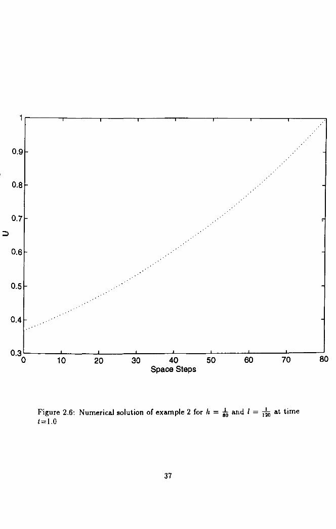
2.6 Numerical solution of example 2 for h = io and I = l~O at
time t=1.0 . . . . . . . . . . . . . . . . . . . . . . . . . . . . . 37
2.7 Theoretical solution of example 2 at time t=1O.0 . 38
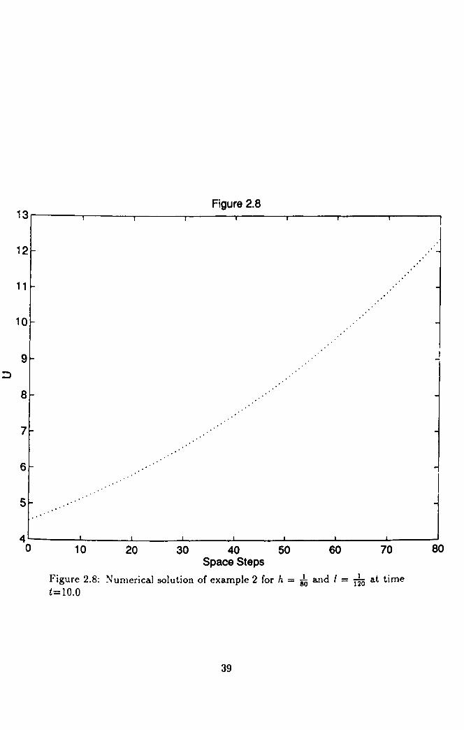
2.8 Numerical solution of example 2 for h = io and I = I~O at
timet=lO.O ............................ 39
2.9 Theoretical solution of Non-Linear Problem at t=lS. 40
2.10 Numerical solution of Non-Linear Problem using h=O.l and
r=1.0 at t=lS. .......................... 41
V 111

3.1 Numerical solution of example 1 for k = 2, h = 6!0 and I = io at time t=0.5 . . . . . . . . . . . . . . . . . . . . . . . .. , 67
3.2 Numerical solution of example 1 for k = 4, h = s!o and I = io at time t=IO.0. . . . . . . . . . . . .. ......... 68
3.3 Numerical solution of example 2 for h = io and 1 = 1;0 at
time t=I.0 . . . . . . . . . . . . . . . . . . . . . . . . . . . . . 69
3.4 Numerical solution of example 2 for h = io and I = rio at
time t=10.0 . . . . . . . . . . . . . . . . . . . . . . . . . . .. 70
4.1 Theoretical solution of example 1 for time t=0.5 . . . . . . . . 83
4.2 Numerical solution of example 1 for h = 0.1, and 1 = 0.1 at
time t=0.5 . . . . . . . . . . . . . . . . . . . . . . . . . . . . . 84
5.1 Numerical solution of example 1 for h = 0.1, and I = 0.1 at
time t=0.5 ............................. 101
6.1 Theoretical solution of example 1 for time t=1.0 ........ 116
6.2 Numerical solution of example 1 for h = 0.1, and I = 0.1 at
time t=1.0 . . . . . . . . . . . . . . . . . . . . . . . . . . .. 117
6.3 Theoretical solution of example 2 for time t=0.5 . 118
6.4 Numerical solution of example 2 for h,I=0.05 at time t=0 .. 5 . . 119
7.1 Numerical solution of example 1 for h, 1= 112 at time t=1.0 . 133
7.2 Numerical solution of example 1 for h, I = 214 at time t=0.5 . 134
IX
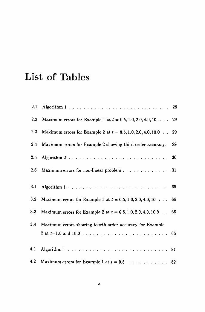
List of Tables
2.1 Algorithm 1 . . . . . . . . . . . . . . . . . . . . . . . . . 28
2.2 Maximum errors for Example 1 at t = 0.5,1.0,2.0,4.0, 10 29
2.3 Maximum errors for Example 2 at t = 0.5,1.0,2.0,4.0,10.0 29
2.4 Maximum errors for Example 2 showing third-order accuracy. 29
2.5 Algorithm 2 . . . . . . . . . . . . . . . . . . . . . . . . . . .. 30
2.6 Maximum errors for non-linear problem. . . . . . . . . . . . . 31
3.1 Algorithm 1 . . . . . . . . . . . . . . . . . . . . . . . . . 65
3.2 Maximum errors for Example 1 at t = 0.5, 1.0,2.0,4.0, 10 66
3.3 Maximum errors for Example 2 at t = 0.5,1.0,2.0,4.0,10.0 66
3.4 Maximum errors showing fourth-order accuracy for Example
2 at t= 1.0 and 10.0 . . . . . . . . . . . . . . . . . . . . . . . . 66
4.1 Algorithm 1 . . . . . . . . . . . . . . . . . . . . . . . . . . . . 81
4.2 Maximum errors for Example 1 at t = 0.5 ........... 82
x

5.1 Algorithm 1 99
5.2 Maximum errors for Example 1 at t = 0.5 100
6.1 Algorithm 1 114
6.2 Maximum absolute errors for Example 1 115
6.3 Maximum absolute errors for Example 2 115
7.1 Algorithm 1 131
7.2 Maximum absolute errors for Example 1. 132
7.3 Maximum absolute errors for Example 2. 132
Xl

Chapter 1
Preliminaries
1.1 Introduction
With the increasing availability of powerful computing machines and the im
provement in numerical techniques finite difference methods are being used
more and more in the solution of physical problems that arise in various
branches of continuum physics such as heat flow, diffusion, fluid dynamics,
magneto-fluid dynamics, electromagnetism, wave mechanics, radiation trans
fer, neutron transfer, elastic vibrations ([IJ, [33]), medical fluid dynamics,
bioengeering, soil physics and chemistry [1] and population dynamics [16].
In the description of these physical problems partial differential equations
and systems of such equations appear which involve two or more indepen
dent variables that determine the behaviour of the dependent variable.
It is often useful to classify partial differential equations into two kinds:
steady-state equations (for example, the Poisson equation and the bihar
monic equation) and evolutionary equations which model systems that un
dergo change as a function of time and they are important inter alia in the
1
description of wave phenomena, thermodynamics, diffusive processes and
population dynamics [16].
According to a natural classification of partial differential equations de
pending upon characteristic directions a partial differential equation may be
elliptic, parabolic or hyperbolic (see [35], [41], etc). Elliptic equations are of
the steady-state type whilst both parabolic and hyperbolic partial differential
equations are evolutionary (unsteady).
The method of characteristics (see [35], [41], etc) is undoubtedly the
most effective method for solving hyperbolic equations in one space dimen
sion, but loses its impact in higher dimensions where it is less satisfactory
[5], and where, therefore, finite differences still have a role to play. So in
the last two decades much attention has been given in the literature to the
development, analysis and implementation of stable and accurate methods
for the numerical solution of partial differential equations with mixed initial
and boundary conditions specified.
There are many forms of model hyperbolic partial differential equations
that are used in analysing various finite difference methods. These range
from simple one-dependent variable first-order partial differential equations
through multiple dependent-variable second-order partial differential equa
tions with as many as three space variables [23]; for example, finite-difference
methods for the wave equation are used in [4), [9], [11], [12], [24], [27], [30],
[34), [40], [47], [49], and [50] and accurate methods for first-order hyperbolic
partial differential equations are developed in [5], [20] and [31].
In this thesis third- and fourth-order numerical methods for the solution
of hyperbolic partial differential equations which do not require complex
2

arithmetic will be developed and tested on well-known problems with exact
solutions known.
1.2 Method of Lines
Covering the region, in which a numerical solution is to be solved, by a rec
tangular grid with sides parallel to the axes and then replacing the spatial
derivatives in the partial differential equation by their finite-difference ap
proximations, thus transforming the partial differential equations, is called
the Method of Lines. Time-dependent problems in Partial Differential Equa
tions (PDEs) are often solved by the Method of Lines (MOL). By this method
the initial/boundary-value problem is transformed into an initial-value in sys
tem form; it can be written in vector-matrix form and its solution satisfies
a recurrence relation. Then numerical methods are developed using suitable
approximations in this recurrence relation.
1.3 Rational Approximations to exp( t )
Several algorithms for the numerical solution of partial differential equations
can be generated through an approximation to the elementary function ap
pearing in the recurrence relation, which is satisfied by the exact solution of
the initial value problem. The use of rational functions for this purpose has
a long and rich history (see, for example, [4], [5J, [27J, [32J, [38J, [39J, [47J,
[54J and referrences therein). Perhaps the most well known and frequently
used are the Pade approximants due to their order and/or stability proper
ties. But methods for solving partial differential equations corresponding to
higher-order Pade approximations entail the use of complex arithmetic in a
3

splitting context. Third- and fourth-order,L-acceptable rational approxima
tions to exp(t), introduced by Taj and Twizell in [38] and [39], which possess
real and distinct poles are given, for a real scalar t, as
and
1 + (1 - a)t + (i - a + b )t2
E3(t) = 1 _ at + bt2 - (~ - ~ + b)t3 ( 1. 1 )
1 + (1 - a)t + (1 - a + b)t2 + (1 - .!! + b - c)t3
E (t) = 2 6 2 ( 1. 2 ) .. 1 - at + bt 2 - ct3 + (_...L + .!! - k + C)t4 24 6 2
in which a, b and c are real numbers, respectively. The error constants for
these rational approximations are
1 a b -- + - --832
and 1 abc
- 30 + 8 - 3 + 2 respectively. These approximations to exp(t) will playa particular role in
later chapters.
1.4 Notations
Usually the theoretical solution of a hyperbolic partial differential equation
is denoted by u and the theoretical solution of a finite-difference equation is
denoted by V, while the computed solution is denoted by {;. The position
at which the solution is taken is shown by appropriate indices, for example,
u~ denotes the theoretical solution of a certain hyperbolic partial differential
equation in one space dimension at mesh point (x, t) = (mh, nl) and V::,
denotes the theoretical solution of a finite-difference scheme at the same
mesh point. A description of each mesh used in this thesis is given as it is
introduced.
4
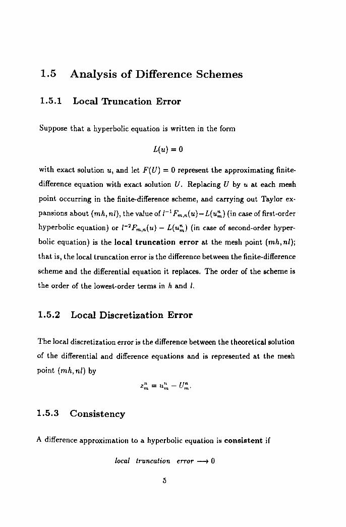
1.5 Analysis of Difference Schemes
1.5.1 Local Truncation Error
Suppose that a hyperbolic equation is written in the form
L(u) = 0
with exact solution u, and let F( U) = 0 represent the approximating finite
difference equation with exact solution U. Replacing U by u at each mesh
point occurring in the finite-difference scheme, and carrying out Taylor ex
pansions about (mh, nl), the value of I-I Fm.n{u)- L{ u:!,) (in case of first-order
hyperbolic equation) or /-2Fm,n{u) - L(u::.) (in case of second-order hyper
bolic equation) is the local truncation error at the mesh point (mil, nl);
that is, the local truncation error is the difference between the finite-difference
scheme and the differential equation it replaces. The order of the scheme is
the order of the lowest-order terms in h and I.
1.5.2 Local Discretization Error
The local discretization error is the difference between the theoretical solution
of the differential and difference equations and is represented at the mesh
point (mh, nl) by
z~ = u~ - U~.
1.5.3 Consistency
A difference approximation to a hyperbolic equation is consistent if
local truncation error ~ 0
5
as space and time steps are refined.
1.5.4 Stability
A finite difference scheme used to solve a P DE is said to be stable if the
difference between the theoretical solution of the difference equation and the
solution actually obtained at the mesh point (mh, nl) remains bounded as n
increases, for fixed h, I and h, 1 --+ 0 for a fixed value of t = nl. The concept
of stability is concerned with the boundedness of the solution of the finite
difference equation (Twizell [41]) and this is examined by finding conditions
under which
zn = un - {;n m m m
remains bounded as n increases for fixed h, I.
There are two methods which are commonly used for examining this na
tion of stability of a finite difference scheme for hyperbolic partial differential
equations namely, the von Neumann Method and the Matrix Method.
(a) The von Neumann Method
Consider the local discretization error
zn = un - ir m m m
and introduce the error function at a given time level t
where (3 is real and a is, in general, complex, such that
z~ = G(x,t) # O.
To investigate the error propagation as t increases, it is necessary to find a
solution of the finite-difference equation which reduces to eifh: when t = O.
6
Let such a solution be
The original error component will not grow with time if
for all a. This is von Neumann's necessary condition for stability. Here the
quantity
is called the amplification factor.
(b) The Matrix Method
The totality of difference equations connecting values of U at two neighbouring
time levels can be written in the matrix form
( 1. 3 )
where Uk(k = n - l,n,n + 1) denotes the column vector
lut, U;, ... ,u~f,
b n is a vector which depends on the boundary conditions and D, B, C are
square matrices of order N (where N is the number of mesh points at each
time level). In the case of a differential equation with constant coefficients the
matrices D, B, C are constant, in the case of a variable coefficients problems,
the matrices D, B, C are evaluated at times (n+ 1)/, nl, (n-1)! respectively.
Wri ting (l.1) in the form
follows that a perturbation ZO of the initial conditions will satisfy
zn+l = D-1 BZn + D-1CZn - 1.
7

This may be written as
[ zn+I]=[D-IA D-IC][ zn] zn I 0 zn-l ( 1. 4 )
which is of the form
where II . " denotes a suitable norm. The necessary and sufficient condition
for the stability of a scheme based on a constant time step and proceeding
indefini tely in time is
II w II~ 1,
for all n, and so the stability condition for the difference scheme, used III
this way, depends on obtaining a suitable estimate for " W ". When W is
symmetric,
where A.(S = 1,2, ... , N) are the eigenvalues of W and II . 112 denotes the
L2-norm. Here, max. I ,X. I is the spectral radius of W and W is called the
amplification matrix.
1.5.5 Convergence
A finite-difference method for hyperbolic partial differential equations is said
to be convergent if the local discretization error
at the fixed mesh point (xm, tn), tends to zero as the mesh is refined by letting
h, I -t 0 simultaneously. In carrying out the convergence analysis, it may be
8

convenient to assume that h and I do not tend to zero independently but
according to a relationship of the form
I = rho,
where r is a constant and Q ~ 1 is some parameter.
9

Chapter 2
Third-Order Numerical Methods for the Advection Equation
2.1 Introduction
There are many finite-difference approximations which can be used to develop
numerical methods for first-order hyperbolic partial differential equations of
the type
8u(x, t) A 8u(x, t) = 0 A 0 at + ax ' >, ( 2. 1 )
with appropriate initial and boundary conditions specified. For example,
central-difference approximations for Ut and U,r, or alternatively a forward
difference approximation for U,r and a central-difference approximation for
ut,etc, can be used. But in this chapter only the space derivative in the par
tial differential equation (2.1) is replaced by new third-order finite-difference
approximations resulting in a system of first-order ordinary differential equa
tions. The solution of this system satisfies a recurrence relation. The accu
racy in time is controlled by choosing a third-order approximation (intro-
10
duced by Taj and Twizell [38]) to the matrix exponential function and after
wards a parallel algorithm is developed and tested on well-known problems
with exact solutions are already known in the literature.
2.2 The Model Problem
A typical problem in applied mathematics consisting of the first-order hy
perbolic partial differential equation is the advection equation. This initial/
boundary-value problem (rBVP) is given by
au(x, t) A au(x, t) = 0 at + ax '
A > 0, x > 0, t > 0 ( 2. 2 )
with the boundary conditions
u(O, t) = I(t), t > 0 ( 2. 3 )
and the initial condition
u(x,O) = g(x), x ~ ° ( 2. 4 )
where g(O) = /0(0) and g(x) is a given continuous function of x. There
will exist a discontinuity between the initial-condition and the boundary
condition at origin if
g(O) =f /0(0).
2.3 The Method
Suppose that the solution u(x, t) of {(2.2)-(2.4)} is to be determined in some
arbitrary region R = [0 $ x ~ XJ x [t > OJ. Dividing the interval [0, XJ into
N subintervals each of width h, so that N h = X, and the time variable
11

t into time steps each of length I gives a rectangular mesh of points with
co-ordinates
(m = 0,1,2, ... , N and n = 0,1,2, ... ) covering the region R = [0 < x <
X] x [t > 0] and its boundary 8R consisting of the lines x = 0, x = X and
t = O.
To approximate the space derivative in (2.2) to third-order accuracy at
some general point (x, t) of the mesh, assume that it may be replaced by the
four-point formula
8u(x, t) 8x
1 = h {a u(x, t) + bu{x - h, t) + eu(x - 2h, t)
+ du(x - 3h,t)}. ( 2. 5 )
Expanding the terms u(x - h, t), u(x - 2h, t) and u(x - 3h, t) as Taylor series
about (x, t) in (2.5) gives
h 8u(x, t) = (a+b+e+d)u(x,t)
8x
+ (-b - 2e - 3d) h 8u(x, t) 8x
+ ~(b 4 9d) h'l8'lu(x, t) 2! + e + 8x2
+ ~(-b - Be _ 27d) h3 ff'u(x, t) 3! 8x3
+ -.!.(b + I6e + BId) h4 {)4U(X, t) 4! 8x4
+ O(hri) as h -+ O. ( 2. 6 )
Equating powers of hi(i = 0, 1,2,3) in (2.6) gives
a + b+ e+ d = 0,
-b - 2e - 3d = 1,
12

b + 4c + 9d = 0, ( 2. 7 )
-b- Be - 27d O.
The solution of the linear system (2.7) is
Thus
ou(x, t) ox
11 3-1 a = 6' b = -3, c = 2' d = T· ( 2. 8 )
1 - 6h {-2u(x - 3h, t) + 9u(x - 2h, t) - 18u(x - h, t)
h3 ()'4u{x i) + llu(x,t)} +"4 ox'" + O(h4) as h --+ 0 ( 2. 9)
is the desired third-order approximation to the first-order space derivative at
(x, i).
Equation (2.9) is valid only for (x, i) = (xm, tn) with Tn = 3,4, ... , N.
To attain the same accuracy at the end points (Xl, tn) and (Xl, in), special
formulae must be developed which approximate ou( x, t) / ax not only to third
order but also with dominant error term ~h304u(x, i)/ax4 for x = Xl, X2 and
t = tn. To achieve both of these, five-point formulae will be needed in
each case. Consider, then, the approximation to ou(x, t)/ox at the point
(x, i) = (xt, in): let
6h ou(x, t) = ax
a u(x - h, t) + bu(x, i) + eu(x + h, i)
3 ()4u(x,i) + du(x+2h,i)+eu{x+3h,t)+-h4 a"
2 x
+ O(h5) as h --+ O. ( 2. 10 )
Then expanding the terms u{x - h, t), u(x + h, t), u(x + 2h, t) and u(x + 3h, t)
as Taylor series about the point (x, t) gives
6h au(x, t) = ax
(a + b + c + d + e) u( x, i)
13

au(x, t) + (-a + c + 2d + 3e) h ax
1 a2u(x,t) + ,(a+c+4d+ge)h2 a 2 2. x
~(- 8d 27 )h3iJ3U(x,t) + 3! a + c++ e ax3
1 8"u(x t) + ,(a + c + I6d + 81 e + 36) h" a" 4. x
+ O(h5) as h ~ O. ( 2. 11 )
Equating powers of hi(i = 0,1,2,3,4) in (2.11) gives
a+b+c+d+e = 0,
-a + c + 2d + 3e = 6,
a + c + 4d + ge = 0, ( 2. 12 )
-a + c + 8d + 27 e = 0,
a + c + I6d + 8Ie = -36.
The solution of the linear system (2.12) is
a = -3, b = 1, c = 0, d = 3, e = -1. ( 2. 13 )
Thus, at the mesh point (Xl! tn), the desired third-order approximation to 8,,(zo,t) • h d . ", 84 ,,(.,t) .
8zo WIt omlDant error term.. 8zo IS
au(x, t) ax
1 = 6h {-3u(x - h, t) + u(x, t) + 3 u(x + 2h, t) - u(x + 3h, t)}
+ h3
8"u(x, t) O(h") h 0 ( 2. 14 ) 4 ax" + as ~.
Suppose, now, that at the point (x, t) = (X2, tn) the approximation to
the first-order space derivative au(x, t)/ax is given by
6h ou(x, t) = a u(x - 2h, t) + bu(x - h, t) + cu(x, t) ax
3 a4u(x,t) + du(x+h,t)+eu(x+2h,t)+2 h4 ax4
+ O(h5) as h ~ O. ( 2. 15 )
14
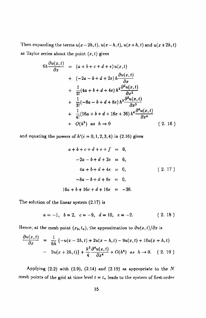
Then expanding the terms u(x-2h, t), u(x-h,t), u(x+h, t) and u(x+2h, t)
as Taylor series about the point (x, t) gives
6h au(x, t) = (a + b + c + d + e) u(x, t) ax
+ au(x, t)
( - 2a - b + d + 2e) h ax
1 a 2u(x t) + ,(4a+b+d+4e)h2 a 2' 2. x
+ 2.( -8a - b + d + 8e) h3lJ3U(X, t) 3! ax3
1 fru(x t) + ,(16a + b + d + 16e + 36) h4 a" 4. x
+ O(h5) as h -.. ° and equating the powers of hi(i = 0,1,2,3,4) in (2.16) gives
a + b + c + d + e + f = 0,
-2a-b+d+2e - 6,
4a + b + d + 4e = 0,
-8a - b + d + 8e 0,
16a + b + 16c + d + 16e = -36.
The solution of the linear system (2.17) is
a=-I, b=2, c=-9, d=10, e=-2.
( 2. 16 )
( 2. 17 )
( 2. 18 )
Hence, at the mesh point (X2' tn), the approximation to {)u(x, t)/8x is
au(x, t)
ax 1
= 6h {-u(x - 2h, t) + 2u(x - h, t) - 9u(x, t) + 10u(x + h, t)
h3 a4u(x t) - 2u(x + 2h, t)} +"4 ax; + O(h4) as h -.. o. (2. 19 )
Applying (2.2) with (2.9), (2.14) and (2.19) as appropriate to the N
mesh points of the grid at time level t = in leads to the system of first-order
15
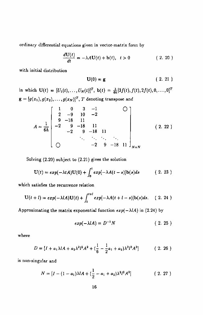
ordinary differential equations given in vector-matrix form by
~;t) = -,xAU(t) + b(t), t > 0 ( 2. 20 )
with initial distribution
U(O) = g ( 2. 21 )
in which U(t) = [Udt), ... ,UN(t)f, b(t) = 6Ah[3f(t),f(t),2f(t),0,,,.,O]T
g = [g(Xt),g(X2),'" ,g(XN)]T, T denoting transpose and
1 0 3 -1 0 2 -9 10 -2 9 -18 11
1 -2 9 -18 11 ( 2. 22 ) A=-6h -2 9 -18 11
0 -2 9 -18 11 NxN
Solving (2.20) subject to (2.21) gives the solution
U(t) = exp( -,xtA)U(O) + l' exp[-,xA(t - s)]b(s)ds ( 2. 23 )
which satisfies the recurrence relation
11+1
U(t + l) = exp(-,xlA)U(t) + 1 exp[-,xA(t + /- s)]b(s)ds. ( 2. 24 )
Approximating the matrix exponential function exp( -MA) in (2.24) by
exp( -,xIA) = D- ' N ( 2. 25 )
where
( 2. 26 )
is non-singular and
( 2. 27 )
16
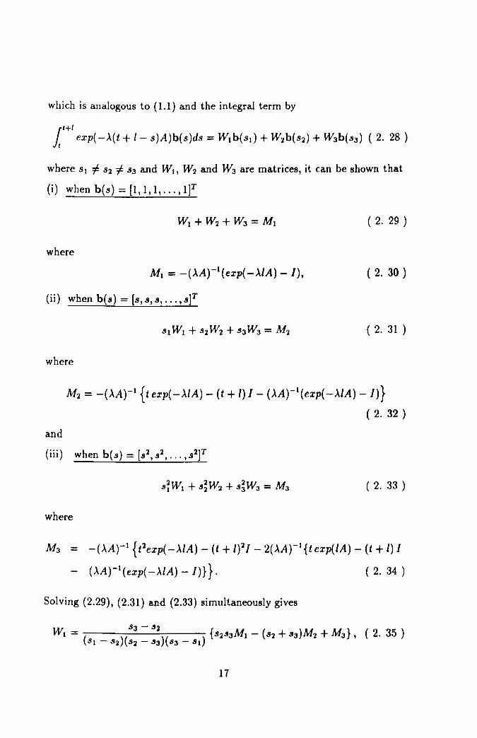
which is analogous to (1.1) and the integral term by
where 81 =f 82 =f 83 and WI, W2 and W3 are matrices, it can be shown that
(i) when b(s) = [1,1,1,.", IJT
( 2. 29 )
where
Ml = -(..\Atl(exp( --\IA) -/), ( 2. 30 )
(ii) when b(s) = [s,s,s,,,.,slT
( 2. 31 )
where
M2 = -(-\Atl {t exp( --\IA) - (t + I) 1- (-\Atl(exp( --\IA) -/)}
( 2. 32 )
and
(iii) when b(s) = [s2,s2, ... ,s2JT
( 2. 33 )
where
M3 = _(-\Atl {t 2exp(--\IA) - (t + /)2/_ 2(-\A)-I{tcxp(lA) - (t + J) I
- (-\A)-l(exp(--\IA) - I)}}. ( 2. 34 )
Solving (2.29), (2.31) and (2.33) simultaneously gives
17
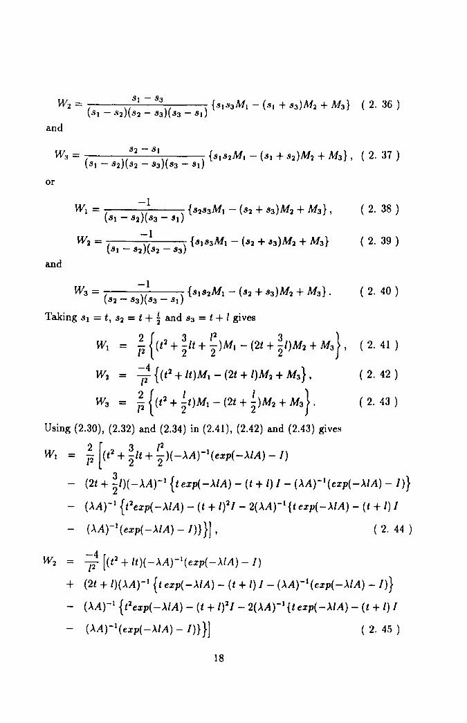
and
or
and
-1 W3 = ( )( ) {8182Ml - (82 + 83)M2 + M3} .
82 - 83 83 - 81
Taking 81 = t, 82 = t + ~ and 83 = t + 1 gives
WI - ~ {(t2 + ~It + ~ )MI - (2t + ~/)M2 + M3} ,
W2 - ~; {(t2 + It)Ml - (2t + I)M2 + M3} I
2{ 2 I (I } W3 = /2 (t +'2 t )MI - 2t+'2)M2+M3 .
( 2. 38 )
( 2. 39 )
( 2. 40 )
( 2. 41 )
( 2. 42 )
( 2. 43 )
Using (2.30), (2.32) and (2.34) in (2.41), (2.42) and (2.43) gives
W 2 [2 3 /2 1 I = J2 (t + '2/t + "2)( -~A)- (exp( -~/A) - I)
- (2t + ~/)( _~Atl {t exp( -~IA) - (t + I) I - (~A)-l (exp( -~/A) - I)}
- (~A)-l {t2exp(-~IA) - (t + 1)2/_ 2(~Atl{texp(-~/A) - (t + I) I
- (~Arl(exp(-~/A) - In}] , (2. 44 )
-4( W2 = [2 (t 2 + 1t)(-~A)-l(exp(-~IA) - I)
+ (2t + /)(AA)-I {t exp( -AlA) - (t + I) I - (~A)-1 (exp( -~/A) - I)}
- (~A)-l {t2exp( -~IA) - (t + 1)21 - 2(AAtl {t exp( -MA) - (t + I) I - (~A)-l(exp(-MA) - In}] ( 2. 45 )
18

and
W 2 [2 I J2 1 3 = i2 (t + 2t + "2)( -AA)- (exp( -AlA) - I)
or
+ (2t + ~)(AAtl {texp(-AIA) - (t + 1)1 - (AA)-l(exp(-AIA) - I)}
- (AA)-l {t2exp( -AlA) - (t + 1)21 - 2(AAt l {t exp( -AlA) - (t + I) I
- (AA)-l(exp( -AlA) - In}] ( 2. 46 )
2 [ 3 12 WI - [2((AAtI)3 _(t2 + 2ft + "2)(AAfZ(exp(-AIA) - I)
+ (2t + ~/)(AA)2 {t exp( -AlA) - (t + I) I - (AAtl(exp( -AlA) - I)} - (AA)2 {t2exp(IA) - (t + 1)2 1- 2(AA)-1{t exp( -AlA) - (t + I) I
- (AAtl(exp( -AlA) - In}] I ( 2. 47 )
W2 = ~24((AAtl)3 [_({Z + It)(AA)2(exp(-AIA) - I)
and
+ (2t + I)(AA)2 {t exp( -AlA) - (t + I) I - (AAtl(exp( -AlA) - I)}
- (AA)2 {t2exp(lA) - (t + 1)2 I - 2(AAtl {t exp( -AlA) - (t + /) I
- (AA)-l(exp( -AlA) - I)}}] ( 2. 48 )
2 [ I 12 W3 - [2(A-1)3 _(t 2 + 2t + "2)A2(exp(IA) - I)
+ (2t + ~)(AA)2 {t exp( -AlA) - (t + I) 1- (AA)-I(exp( -AlA) - I)} - (AA)2 {t 2exp(lA) - (t + 1)21 - 2(AA)-1 {t exp( -AlA) - (t + I) I
- AA)-l (exp( -ALA) - I)}}] . ( 2. 49 )
Then it is easy to show that
2 {A2[2 3Al WI = 12 ((AA)-1)3 -(-2- A2 + TA + 21) exp( -AlA)
19
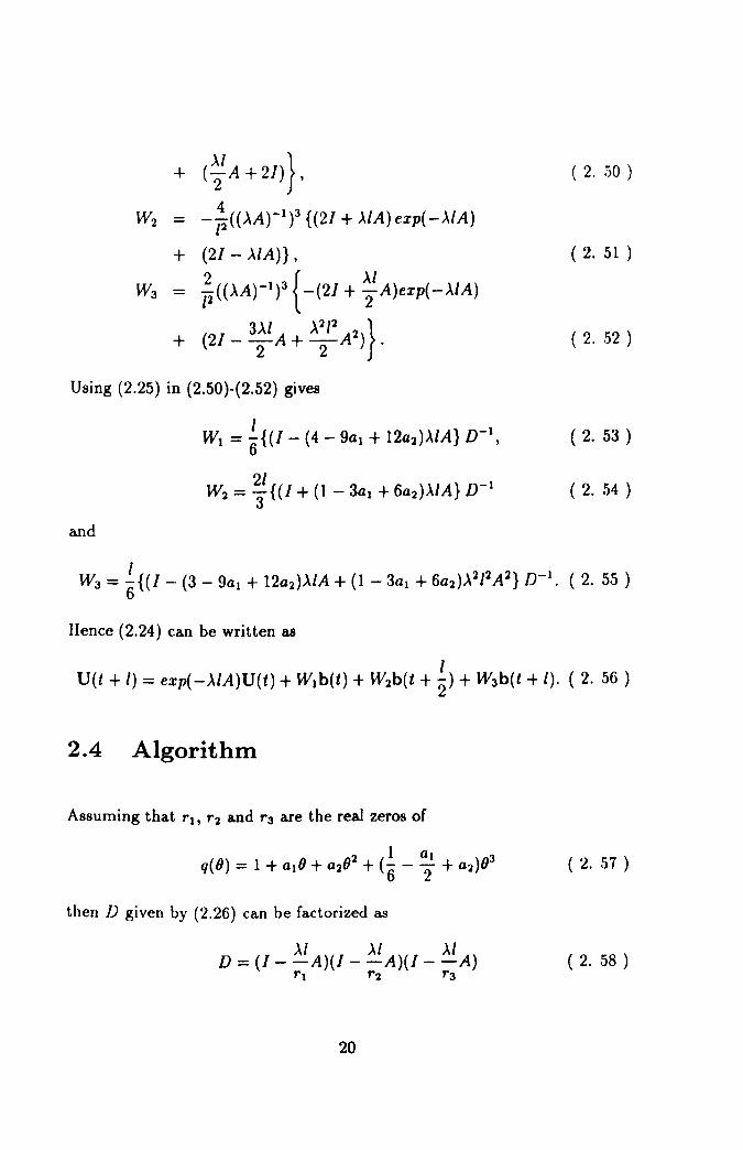
+ (~l A + 21) } ,
W2 = - ~ ((~A)-1)3 ({2/ + ~/A) exp( -~/A)
+ (21 - ~IA)} ,
2 { ~I W3 - 12 ((~Atl)3 -(2/ + "2 A )exp( -~/A)
+ (21 _ 3~1 A + ~2/2 A2)} 2 2 .
Using (2.25) in (2.50)-(2.52) gives
WI = ~{(1 - (4 - 9al + 12a2)~/A} D- I,
W2 = ~I {(I + (1 - 3a1 + 6a2)~/A} D- I
and
Hence (2.24) can be written as
( 2 .. jO )
( 2. 51 )
( 2. 52 )
( 2. 53 )
( 2. 54 )
1 U(t + I) = exp( -~/A)U(t) + Wlb(t) + W2b(t + '2) + W3b(t + I). ( 2. 56 )
2.4 Algorithm
Assuming that rJ, r2 and r3 are the real zeros of
( 2. 57 )
then /J given by (2.26) can be factorized as
~I ~I AI D = (I - -A)(I - -A)(I - -A)
rl r2 r3 ( 2. 58 )
20
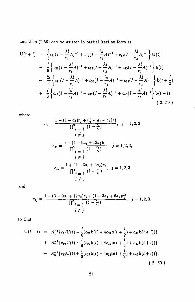
and then (2.56) can be written in partial fraction form as
where 1 - (1 - adrj + (~ - al + a2)rJ
elj = n3. (1 _ !:J.) , z = 1 r,
j = 1,2,3,
ii=j 1 - (4 - gal + 12a2)rj
c2i = n3 . (1 _ ~ ) , 1 = 1 r,
j = 1,2,3,
ii=j 1 + (1 - 3al + 6a2)rj
c3i = n3 . (1 _ !:J.) , 1 = 1 r,
j = 1,2,3
i i= j
and
c . _ 1 - (3 - gal + 12a2)ri + (1 - 3al + 6a2)rl 4) - n3. (1 _ ~) , , = 1 r,
j = 1,2,3.
i i= j
so that
21

where
or
where
Let
then
>'1 Ai=/--A, i=1,2,3,
rj
3
U(t + l) = L A;-IZi i=1
A -I i Zi = Yi
in which Yl, Y2 and Y3 are the solutions of the systems
AiYi = Zi, i = 1,2,3.
( 2. 61 )
( 2. 62 )
( 2. 63 )
( 2. 64 )
respectively. This algorithm is presented in tabular form in Table 2.1.
2.5 Numerical Examples
In this section only a representative of many other methods based on (2.25)
will be used. So taking
and
65431 al = 50000
171151 a2 = 300000
Taj and Twizell [38], which give a very small local truncation error, gives
rl = 2.18837132239, r2 = 2.33987492248, r3 = 2.35690139372
22

as the real zeros of (2.57). These values produce
Cll = -176.185066638, Cn = 2051.11129521, el3 = -1873.92622858,
C2l = -224.317807049, C22 = 2358.75587416, C23 = -2133.43806711,
C3l = -19.0008161810, C32 = 326.498892802, C33 = -306.498076621,
C41 = -182.736963963, C42 = 1594.78928297, C43 = -1411.05231901
2.5.1 Example 1
Consider the one space variable partial differential equation
ou + ou _ 0 0 < x < 1, t > O. at ax - , subject to the boundary conditions
u(O, t) = -sin(2k1rt), t > 0,
where k is a positive integer and the initial condition
u(x,O) = sin(2k1rx), 0 ~ x ~ 1.
This problem has theoretical solution
u(x, t) = sin{2k1r(x - t)}
( 2. 65 )
( 2. 66 )
( 2. 67 )
( 2. 68 )
(see Oliger [31]). The integer k gives the number of complete waveR in the
interval ° ~ x ~ 1. Using the algorithm developed in section 2.4 with
the information given at the beginning of this section, the problem ((2.65)
(2.67)} is solved for h = s.!o and I = io so that r = 8.0(r = k), using k = 2
and 4 and compared with the results obtained by Arigu et al. [5J whose
algorithm requires the use of complex arithmetic. The theoretical solutions
23

and the numerical solutions for k = 2 and k = 4 at time t = 0.5 and
t=lO.O respectively are depicted in Figure 2.1 - 2.4. In these experiments the
method behaves smoothly over the whole interval 0 ::; x ::; 1 and no contrived
oscillations are observed. The apparent decay in amplitude in Figure 2.4 is
due to the build-up of round-off errors. Maximum errors at time t=O.5, 1.0,
2.0, 4.0, 10.0, are given in Table 2.2.
2.5.2 Example 2
Consider again the one space variable partial differential equation
au au at + ax = 0, 0 < x < 1, t > O. ( 2. 69 )
subject to the boundary conditions
u(O,t) = e- t, t > 0, ( 2. 70 )
and the initial condition
( 2. 71 )
This problem has theoretical solution
u(x,t) = er-
t ( 2. 72 )
(see Arigu et al. [5]), which decays as time increases. Using once again
the algorithm developed in Section 2.4 with the information given at the
beginning of this section the problem {(2.69)-(2. 71)} is solved for h = 8~ and I = l~O and compared once again with the results obtained by Arigu
et al. [5]. In these experiments the method behaves smoothly over the
whole interval 0 ::; x ::; 1 and no contrived oscillations are observed. From
Table 2.3 it is clear that accuracy of this method is much much better than
24

the O(h2 + [4) method of Arigu et al. From Table 2.4 it is also clea.r tha.t
the method is third-order at time t=l.O and 10.0 because, as h and I are
both successively halved, the errors decrease in magnitude by a factor of
8( approximately). Theoretical and numerical solutions at time t= 1.0, 10.0
are depicted in Figure 2.5 - 2.8. Maximum errors at time t=0.5, 1.0, 2.0, 4.0
and 10.0 are given in Table 2.3.
2.6 Non-linear Problem
Consider the first-order non-linear hyperbolic partial differential equation
au ~ au2 _ ° at + 2 ax - , ,O$x$X, t>O ( 2. 73 )
where u = u(x, t), which is ubiquitous in wave theory and in quantum me
chanics, with the boundary conditions
u(O, t) = f(t), t > 0 ( 2. 74 )
and the initial condition
u(x,O) = g(x), 0:5 x :5 X ( 2. 7.5 )
where g(x) is a given continuous function of x. There will exist a discontinuity
between the initial condition and the boundary condition at the origin if
g(O) 'f f(O}.
Equation (2.73) may be written as
au au at + u ax = 0, 0 :5 x :5 X, t > O. ( 2. 76 )
25
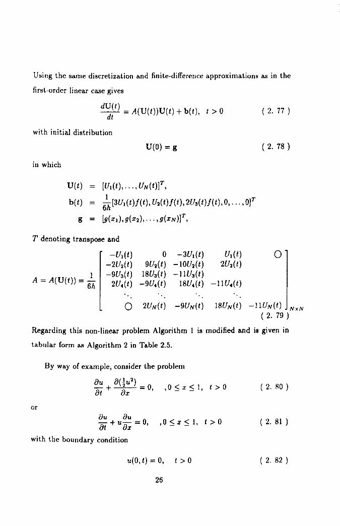
Using the same discretization and finite-difference approximations as in the
first-order linear case gives
dU(t) = A(U(t))U(t) + b(t), t > 0 dt
with initial distribution
U(O) = g
in which
U(t) = [U1(t), ... , UN(t)]T,
b(t) 1 ]T = 6h [3U1(t)f(t), U2(t)f(t), 2U3(t)f(t), 0, ... ,0
g = [g(Xt},g(X2),,,.,g(XN)]T,
T denoting transpose and
1 A = A(U(t)) = -
6h
-U1(t) -2U2(t) -9U3 (t)
2U .. (t)
o 9U2(t)
18U3 ( t) -9U .. (t)
-3U1(t) -lOU2(t) -l1U3 (t)
18U .. (t) -l1U .. (t)
( 2. 77 )
( 2. 78 )
o
o 2UN(t) -9UN(t) 18UN(t) -llUN(t) NxN ( 2. 79 )
Regarding this non-linear problem Algorithm 1 is modified and is given in
tabular form as Algorithm 2 in Table 2.5.
By way of example, consider the problem
au a(~u2) _ 0 at + ax -, ,0 ~ x ~ 1, t > 0 ( 2. 80 )
or au au -+u-=O ,O<_x<_I, t>O at ax ' ( 2. 81 )
with the boundary condition
u(O, t) = 0, t > 0 ( 2. 82 )
26
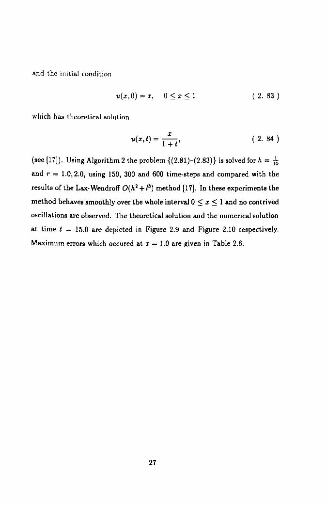
and the initial condition
u(x,O)=x, O~x~l
which has theoretical solution
x u(x, t) = -1-' +t
( 2. 83 )
( 2. 84 )
(see [17]). Using Algorithm 2 the problem {(2.81)-(2.83)} is solved for h = l~
and r = 1.0,2.0, using 150, 300 and 600 time-steps and compared with the
results of the Lax-Wendroff O(h2 + 13 ) method [17]. In these experiments the
method behaves smoothly over the whole interval 0 ~ x ~ 1 and no contrived
oscillations are observed. The theoretical solution and the numerical solution
at time t = 15.0 are depicted in Figure 2.9 and Figure 2.10 respectively.
Maximum errors which occured at x = 1.0 are given in Table 2.6.
21
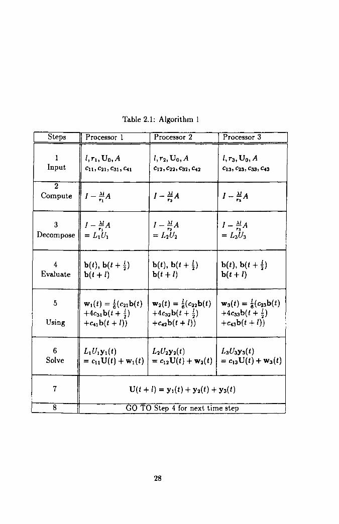
Table 2.1: Algorithm 1
Steps II Processor 1 I Processor 2 I Processor 3
1 /, rl, Vo,A I,r:h Vo, A I, r3, Vo, A Input Cll, C2l! C3l , Cn Cn, C22, C32, C42 C13, C23, C33, c..3
2 Compute / - ,\1 A
rl /-MA
rl /_ .\IA
r3
3 / - ,\1 A / - ,\1 A / - ,\1 A rl rl r3
Decompose = L1Ul = L2U2 = L3U3
4 b(t), b(t + 4) b(t), b(t + 4) b( t), b( t + 4) Evaluate b(t + I) b(t + /) b(t + /)
5 Wl(t) = ~(C21b(t) W2(t) = ~(C22b(t) W3(t) = ~(C23b(t) +4C31 b(t+4) +4C32b(t + 4) +4C33b( t + 4)
Using +c..lb(t + I)) +C42 b(t + I)) +C43b( t -+ /))
6 L1U1Yl(t) L2U2Y2(t) L3 U3Y3(t) Solve = Cll V ( t) + WI ( t ) = cnV(t) + W2(t) = C13V(t) + W3(t)
7 V(t + /) = Yl(t) + Y2(t) + Y3(t)
8 GO TO Step 4 for next time step
28

Table 2.2: Maximum errors for Example 1 at t = 0.5, 1.0,2.0,4.0, 10
It" 0.5 1.0 2.0 4.0 10.0
k=2 -0.6160-3 -0.1100-2 -0.1100-2 -0.1100-2 -0.1100-2
* 0.2710-2 0.2690-1 0.2610-1 0.2600-2 -
k=4 -0.9620-2 -0.1810-1 -0.1810-1 -0.1810-1 -0.1810-1
* - - - - 0.6410-1
* Maximum absolute errors of Arigu et al.[5] O(h2 + P) Method
Table 2.3: Maximum errors for Example 2 at t = 0.5,1.0,2.0,4.0, 10.0
It" 0.5 1.0 2.0 4.0 10.0
-0.3940-6 -0.4500-6 -0.1650-6 -0.2240-7 -0.5550-10
* - -- 0.5110-2 0.2150-4 0.8690-6
* Maximum absolute errors of Arigu et al.[5] O(h'J + 14) Method
Table 2.4: Maximum errors for Example 2 showing third-order accuracy.
h, I " 0.1 0.05 0.025 0.0125
t = 1.0 -0.1920-03 -0.2360-04 -0.3080-05 -0.423D-06
t = 10.0 0.3410-05 0.5570-06 0.8200-07 0.112D-07
29

Table 2.5: Algorithm 2
I Steps Processor 1 Processor 2 Processor 3
1 I, rl! Vo I, r2, Vo I, r3, Vo Input Cn, C2l! C3l, en C12, C22, C3l, e42 C13, C23, C33, C .. 3
2 Update A A A
3 Compute / _ AI A / _ AI A /_ AlA
rl r2 r3
4 / _ AlA / _ AlA / _ AlA rl r2 r3
Decompose = Ll UI = L2U2 = L3U3
5 b(t), b(t + 4) b(t), b(t + 4) b(t), b(t + 4) Evaluate b(t + I) b(t + I) b(t + I)
6 Wl(t) = ~(C21b(t) W2(t) = ~(C22b(t) W3( t) = ~ (C23b( t) +4C3l b(t + 4) +4C32 b(t + 4) +4C33b(t + 4)
Using +C .. l b( t + I)) +C"2b(t + I» +C"3b(t + I»
7 L1U1Yl(t) L2Ul Y2(t) L3U3Y3(t) Solve =CllU(t)+Wl(t) = CI2 U(t) + W2(t) = CI3U(t) + W3(t)
8 U(t + I) = Yl(t) + Y2(t) + Y3(l)
9 GO TO Step 2 for next time step
30

Table 2.6: Maximum errors for non-linear problem
" Time steps I h I r I Maximum absolute errors I • " 150 0.1 1 0.540-03 0.790-03
150 0.1 2 0.360-03 0.380-03
300 0.1 1 0.lBO-03 0.120-02
300 0.1 2 0.110-03 0.610-03
600 0.1 1 0.330-04 -
600 0.1 2 0.660-05 -
* Maximum absolute errors of Lax-Wendroff O(h2 + [3) Method [17](p. 426)
31

0.8
0.6
o
-0.2
-0.4
-0.6
-0.8
_'~ ____ ~ ________ ~ ________ L-~~ ________ ~ ________ L-__ ~ ________ ~~~L-----~
o 0.8 0.9 1 0.2 0.3 0.4 0.5 x
0.6 0.7
Figure 2.1: Theoretical solution of example I for k = 2 at time t=O.5
32

Figure 2.2 1r----,~------~------_r------~------._------r_----_.
0.8
o
-0.2
-0.4
-0.6
-0.8
.... I I
J
-1~------~----~~~~~~----~------~--~~~------~ o 100 200 300 400 500 600 700 Space Steps
Figure 2.2: Numerical solution of example 1 for k = 2, h = &!o and 1= io at time t=O.5
33

Figure 2.3 1
0.8
0.6
0.4
0.2
0
-0.2
-0.4
-0.6
-0.8
-1 0 0.1 0.2 0.3 0.4 0.5 0.6 0.7 0.8 0.9 1
x
Figure 2.3: Theoretical solution of example 1 for k = 4 at time t=10.0
34

Figure 2.4 'r-~----r------'r-----~r---~-.r-----~~----~------~
0.8
0.6
0.4
0.2
o
-0.2
-0.4
-0.6
-0.8
-,--------~~----~----~~------~~~----~------~------~ o 100 200 300 400 500 600 Space Steps
Figure 2.4: Numerical solution of example 1 for k = 4, It = 6!O and I = ~ at time t=10.0
35
700

1r----,r----.----~----_.----_r----_.----,_----._----._--~
0.9
0.8
0.7
0.6
0.5
0.4
0.3~--~----~----L---~----~--~~--~----~--~----~ o 0.1 0.2 0.3 0.4 0.5
x 0.6 0.7 0.8
Figure 2.5: Theoretical solution of example 2 at time t= 1.0
36
0.9 1
1r-------r------,T-------.-I------.-------.-----~------~T------~
0.9'"
0.8~ -
0.7
0.6'"
0.5 -
0.4
0.3~------~----~------~-------~'------L------J------~------~ 80 o 10 20 30 40 50 60 70
Space Steps
Figure 2.6: Numerical solution of example 2 for h = ;0 and I = I~O at time t=l.O
37
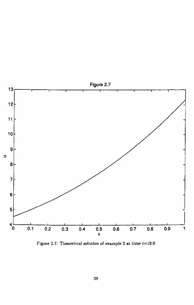
Figure 2.7 13r----.----.---~----_r----r_--~----,_--~r_--_r--__,
4----~~--~----~----~----~----~----~----~--~----~ o 0.1 0.2 0.3 0.4 0.5 x
0.6 0.7 0.8
Figure 2.7: Theoretical solution of example 2 at time t=lO.O
38
0.9 1
13 Figure 2.8
12
11
10
9 ::>
8
7
6
5
4 0 10 20 30 40 50 60 70 80
Space Steps
Figure 2.8: ~umerical solution of example 2 for It = io and I = l~O at time t=10.0
39
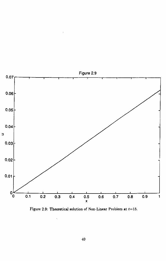
Figure 2.9 0.07r----.----~--_,----_r----._--~----~--_,----_r--~
0.06
0.05
0.04
0.03
0.02
0.01
o----~----~--~----~----~--~----~--~~--~--~ o 0.1 0.2 0.3 0.4 0.5 x
0.6 0.7 0.8
Figure 2.9: Theoretical solution of Non-Linear Problem at t=15.
40
0.9 1

Figure 2.10 0.07 r----,--""T"-----.-----.----r------.---...,..------.----.------.
0.06
0.05
0.04
0.03
0.02
0.01
1 2 3 456 Space Steps
7 8 9
Figure 2.10: Numerical solution of Non-Linear Problem using h=O.1 and r=1.0 at t=15.
41
10

Chapter 3
Fourth-Order Numerical Methods for the Advection Equation
To develop fourth-order numerical methods for first-order hyperbolic partial
differential equations of the type (2.1) with appropriate initial and boundary
conditions specified, the space derivative in the partial differential equation
is replaced by new fourth-order finite-difference approximations resulting in
a system of first-order ordinary differential equations the solution of which
satisfies a recurrence relation. The accuracy in time is controlled by a fourth
order approximation to the matrix exponential function which is introduced
by Taj and Twizell [39].
3.1 The Method
Assume that the combination
au(x - 4h,t) + bu(x - 3h,t) + cu(x - 2h,t) + du(x - h,t) + eu(x,t)
42

gives the fourth-order approximation to ~; at (x, t). Then expanding the
terms u(x - 4h,t),u(x - 3h,t),u(x - 2h,t) and u(x - h,t) as Taylor series
about the point (x,t) gives
a u(x - 4h, t) + bu(x - 3h, t) + cu(x - 2h, t) + du(x - h, t) + e u(x, t)
= (a+b+c+d+e)u(x,t)
ou + (-4a - 3b - 2e - d)h ox
1 o'2u + ,(16a + 9b + 4e + d)h 2
0 '2
2. x 1 3~u + -(-64a - 27b - Be - d)h -3! ox3
1 ~u + ,(256a + BIb + 16e + d)h"
o ..
4. x 1 ~u + -(-1024a - 243b - 32e - d)h 5
-5! ax!>
+ O(h6) as h ~ O. ( 3. 1 )
Equating the powers of hi(i = 0,2,3,4) in (3.1) to zero and the power of h
to 1 gives
e+d+c+b+a = 0
-d - 2c - 3b - 4a = d+4c+9b+16a = 0 ( 3. 2 )
-d - 8e - 27b - 64a = 0
d + 16e + 81 b + 256a = O.
The solution of this linear system is
1 a =-,
4
Thus
-4 b=T' e = 3, d = -4,
25 e =-.
12
1 4'u(x-4h,t) -
4 25 3u(x - 3h, t) + 3 u(x - 2h, t) - 4 u(x - h, t) + 12 u(x, t)
_ h ou _ !hrJ)5u + O(h6) as h -+ O. ( 3. 3 )
ax 5 ax5
43

or
1 12 {3u(x - 4h, i) - 16u(x - 3h, t) + 36u(x - 2h, t) - 48u(x - h, t)
+25u(x, tn ( 3. 4 )
Thus the desired approximation to ~; is given by
au 1 ax - 12h {3u(x - 4h, t) - 16u(x - 3h, t)
+ 36u(x - 2h, t) - 48u(x - h, t) + 25u(x, t)}
1 .. a5u O( Ii) h + 5 h ax5 + h as -+ O. ( 3. 5 )
Equation (3.5) is valid only for (x, t) = (xm, tn) with m = 4,5, ... , N. To
attain the same accuracy at the end point (Xl, tn), (X'l' in) and (X3, in) special
formulae must be devolped which approximate ~; not only to fourth-order
but also with dominant error term lh"~ for X = Xl, X2, X3 and t = tn.
Consider then the approximation to ~; at the point (x, t) = (Xl, tn); let
12h ~: = a u(x - h, t) + bu(x, t) + cu(x + h, t) + du(x + 2h, t)
12 5 a5u + eu(x+3h,t)+f u(x+4h,t)+5 h axs
+ 0(h6) as h -+ O. ( 3. 6 )
Expending the terms u(x - h,t),u(x + h,t),u(x + 2h,t),u(x + 3h,t) and
u( X + 4 h, t) as Taylor series abou t the point (x, t) gi ves
12hau
= (a+b+c+d+e+f)u(x,t) ax
au + ( -a + c + 2d + 3e + 4f)h ax
1 a2u + 2(a+c+4d+ge+16f)h'lax
'l
1 ~u + ii( -a + c + 8d + 27e + 64f)hl axl
1 ~u + 24 (a + c + 16d + 81e + 256f)h" ax"
44
1 12 fl)u + 120 (-a + c + 32d + 243e + 1024/ + 5" )h 5
ax 5
+ O(h6) as h -+ O.
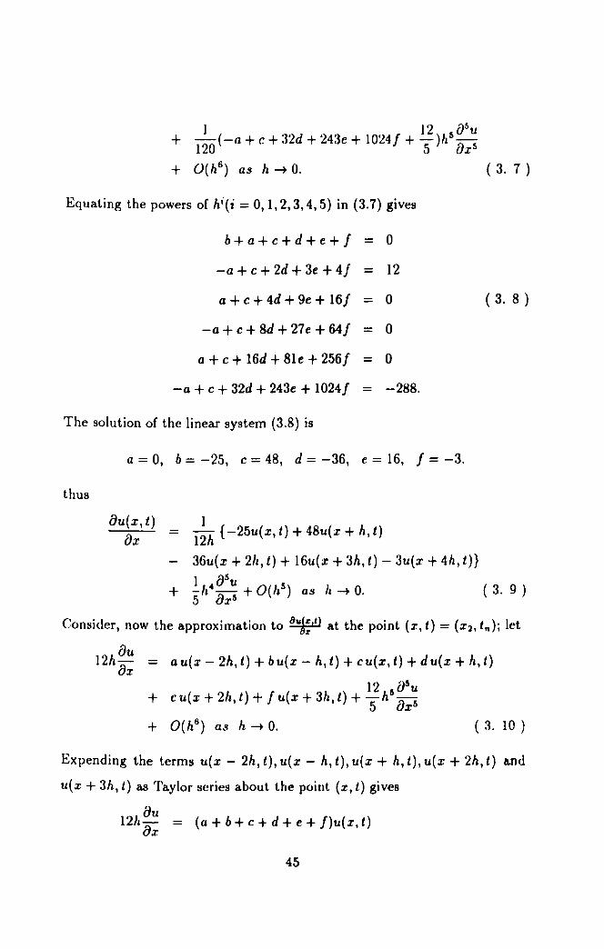
Equating the powers of hi(i = 0,1,2,3,4,5) in (3.7) gives
b+a+c+d+e+/ = 0
-a + c + 2d + 3e + 4/ = 12
a + c + 4d + ge + 16/ = 0
-a + c + 8d + 27 e + 64/ = 0
a + c + 16d + 81 e + 256/ = 0
-a + c + 32d + 243e + 1024/ = -288.
The solution of the linear system (3.8) is
a = 0, b = -25, c = 48, d = -36, e = 16, / = -3.
thus
au(x, t)
ax
1 = 12h {-25u(x, t) + 48u(x + h, t)
( 3. 7 )
( 3. 8 )
- 36u(x + 2h, t) + 16u(x + 3h, t) - 3u(x + 4h, t)}
1 B5u + Sh4 ax5 + O(h5) as h -+ O. ( 3. 9 )
Consider, now the approximation to 8vJ:,t) at the point (x, t) = (X:h tn); let
12h:: = au(x-2h,t)+bu(x-h,t)+cu(x,t)+du(x+h,t)
12 lJ5u + cu(x + 2h,t) + /u(x + 3h,t) + 5' h5 ax5
( 3. 10 )
Expending the terms u(x - 2h, t), u(x - h, t), u(x + h, t), u(x + 2h, t) and
u(x + 3h, t) as Taylor series about the point (x, t) gives
12hBu
= (a+b+c+d+e+f)u(x,t) ax
45

iJu + (-2a - b + d + 2e + 3f)h ax 1 iJ2u
+ 2(4a + b+ d + 4e + 9f)h2 ax2
1 3~u + "6( -8a - b + d + 8e + 27 f)h ax3
1 ~u + 24 (16a + b + d + 16e + 81f)h
4 ox4
1 12 585U + 120 (-32a - b + d + 32e + 243/ + 5")h ax5
+ O(h6) as h --+ O. ( 3. 11 )
Equating the powers of hi(i = 0,1,2,3,4,5} in (3.11) gives the system
c+b+a+d+e+/ = 0
-b - 2a + d + 2e + 3/ = 12
b + 4a + d + 4e + 9/ ::: 0 ( 3. 12 )
-b - 8a + d + 8e + 27/ = 0
b + 16a + d + 16e + 81/ = 0
- b - 32a + d + 32e + 243/ = -288
which has solution
Thus
8u(x, t) ax
a=3, b=-18, c=20, d=-12, e=9, /=-2.
1 = 12h {3u(x - 2h, t) - 18u(x - h, t)
+ 20u(x, t) - 12u(x + h, t) + 9u(x + 211, t) - 2u(x + 311, t)}
1 4 a5u 5 ) + "5 h ax" + O(h } as h --+ O. ( 3. 13
is the desired fourth-<>rder approximation to alt,t) with dominant error term h' 8~u(r.t) . "5 8r5 at the pomt (X2' tn).
46

let
Consider, next the approximation to OUJ:,I) at the point (x, t) = (X3, tn);
12h f)u = f)x
a u(x - 3h, t) + bu(x - 2h, t) + cu(x - h, t) + du(x, t)
12 f)5 u + eu{x + h,t) + /u(x + 2h,t) + 5" h5 f)x 5
+ O(h6) as h ~ O. ( 3. 14 )
Expanding the terms u(x - 3h,t),u(x - 2h,t),u(x - h,t),u(x + h,t) and
u(x + 2h, t) as Taylor series about the point (x, t) gives
12h au ax
= (a + b + c + d + e + f)u(x, t)
au + ( -3a - 2b - c + e + 2f)h-
{)x 1 {)~u
+ -(9a + 4b + c + e + 4f)h~ {) ~ 2 x 1 3~U
+ - ( - 27 a - 8b - c + e + 8 f) h -6 ox3
1 ~u + 24 (81a + 16b + c + e + 16f)h" ax"
1 12 {)6U
+ -(-243a - 32b - c+ e + 32/ + _)h6_
120 5 axt;
+ O(h6) as h ~ O. ( 3. 15 )
Equating the powers of hi(i = 0,1,2,3,4,5) in (3.15) gives
d+e+c+b+a+/ = 0
e - c - 2b - 3a + 2/ = 12
e + c + 4b + 9a + 4/ = 0 ( 3. 16 )
e - c - 8b - 27a + 8/ = 0
e + c + 16b + 81 a + 16/ = 0
e - c - 32b - 243a + 32/ = -288
47

The solution of the linear system (3.16) is
Thus
8u{x, i) Ox
a = 2, b = -9, c = 12, d = -20, c = 18, / = -3.
1 = 12h {2u(x - 3h, t) - 9u{x - 2h, t)
+ 12u(x - h, t} - 20u(x, t) + 18u{x + h, t) - 3u{x + 2h, i)}
1 .. 05U (5) h ( ) + Sh OX5 + 0 h as -+ O. 3. 17
is the desired approximation to But,,) at the point (X3, tn).
Applying (2.2) with (3.5) or (3.9) or (3.13) or (3.17) as appropriate to
the N mesh points at the time level t = nl, leads to the system of first-order
ordinary differential equations given in vector-matrix form as
cIU(t} ---;Jt = -~AU(t) + b(t), t > 0
with initial distribution
in which
U(O) = g
U(t) = [Ul(t), ... , UN(t)]T, b(t) - l;h [0, -3/(t), -2/(t), -3/(t), 0, ... , O]T,
g = [g(xd, g(Xl),'" ,g(XN )]T,
T denoting transpose and
-25 48 -36 16 -3 0 -18 20 -12 9 -2 -9 12 -20 18 -3
I -16 36 -48 2.5 0 A=- 3 -16 36 -48 25 12h
3 -16 36 -48 25
o 3 -16 36 -48 25 NxN
48
( 3. 18 )
( 3. 19 )
( 3. 20 )

It is observed that the matrix A has distinct eigenvalut>s with negative rt>al
parts for N=7, 9, 19 and 39 given in Appendix A.
Solving (3.18) subject to (3.19) gives the solution
U(t) = exp(-..\tA)U(O) + fo' exp[-AA(t - s)]b(s)ds ( 3. 21 )
which satisfies the recurrence relation
1,+1
U(t + l) = exp( -"\IA)U(t) +, exp[-"\A(t + 1- s)]b(s)ds. ( 3. 22 )
Approximating the matrix exponential function exp( -ALA) in (3.22) by
exp( -ALA) = D-1 N ( 3. 23 )
where
is non-singular and
which is analogous to (1.2) and the integral term by
where 81 f; 82 f; S3 f; s" and W), W2 , W3 and W" are matrices, it can be
shown that
(i) when b(8) = (l,l,l, ... ,I)T
( 3. 27 )
where
( 3. 28 )
49
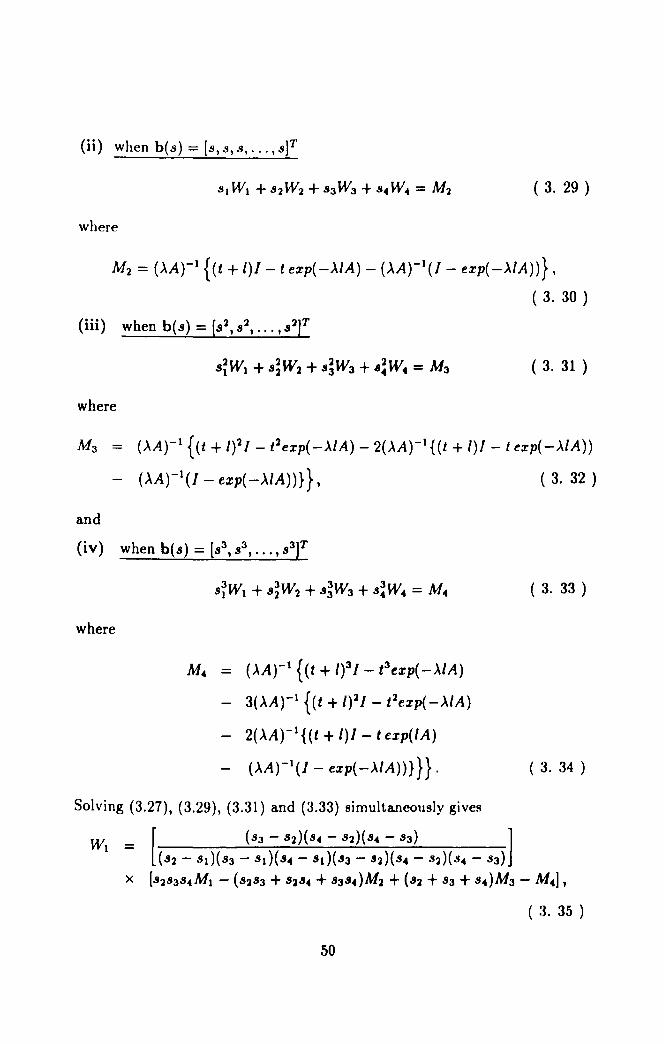
(ii) 1 [ JT Wlen b(8) = 8,8,8, ... ,8
( 3. 29 )
where
M2 = (AAr l {(t + 1)1 - t exp( -ALA) - (AA)-I(l- exp( -ALA»},
( 3. 30 )
( 3. 31 )
where
M3 = (AA)-I {(t + 1)2 I - t 2exp( -ALA) - 2(AAr 1 {(t + 1)1 - t exp( -ALA»
- (AArl(I - exp( -AlA»}} I ( 3. 32 )
and
where
M. = pArt {(t + 1)31- t3exp( -AlA)
- 3(AA)-' {(t + 1)2 I - t'lexp( -AlA)
- 2(AAr' {(t + 1)1 - t exp(lA)
- (AArt(l- exp( -AlA»))}} .
Solving (3.27), (3.29), (3.31) and (3.33) simultaneously gives
WI _ [ (.'13 - .'12)(.'1. - S'l)(s. - .'13) 1 (.'12 - .'1.)(.'13 - sd(s. - Sd(S3 - S'l)(s. - .'12)(.'1. - .'13)
( 3. 33 )
( 3. 34 )
X [S'lS3s.M, - (.'12.'13 + .'12.'1. + s3s.)M'l + (.'12 + .'13 + s.)M3 - M.J, ( 3. 35 )
50
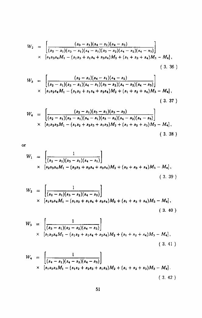
W2 = [ (S3 - sd(s .. - sd(s .. - S3) 1 (82 - 81)(83 - 81)(8 .. - SI)(83 - 82)(84 - 82)(84 - 83)
X [8IS3S .. MI - (SIS3 + SIS .. + s3s .. )M2 + (Sl + S3 + s .. )M3 - M .. J ,
( 3. 36 )
W3 = [ (S2 - S.)(S .. - S.)(S .. - S2) 1 (S2 - S.)(S3 - S.)(S .. - S')(S3 - S2)(S .. - S2)(S .. - S3)
x [SIS2S .. Ml - (SIS2 + SIS .. + s2s .. )M2 + (SI + S2 + s .. )M3 - M .. J ,
( 3. 37 )
W.. _ [ (S2 - S.)(S3 - 8.)(83 - 82) 1 (S2 - Sd(83 - S.)(S .. - 8.)(83 - S2)(8 .. - S2)(84 - 83)
X [SIS2S3Ml - (SIS2 + S283 + 8183)M2 + (81 + 82 + 83)M3 - M .. J ,
( 3. 38 )
or
( 3. 39 )
( 3. 40 )
( 3. 41 )
( 3. 42 )
51

Taking 8] = t, 82 = t + 4, 83 = t + ~I and 8. = t + I give~
W 9 {( 3 2 11 2 2 3 2 11 2 ] = 2/3 t + 2ft + -I t + -I )MI - (3t + 41t + -I )M2 9 9 9
+ {3t + 2l)M3 - M.} , ( 3. 43 )
W2 = -~ {(tJ + ~/t2 + ~/2t)MI - (3t 2 + .!E./t + ~/2)M2 2[3 3 3 3 3
+ (3t + ~/)M3 - M.} , ( 3. 44 )
W 27 {( 3 4 2 1 2 ) (2 8 1 2 J = 213 t + '3 1t + '31 t MI - 3t + '3 ft + '31 )M2
+ (3t + ~/)M3 - M. } , ( 3. 45 )
W 9 {3 2 22) (2 22 4 = - 213 (t + It + 91 t MI - 3t + 2ft + 91 )M2
+ (3t + I)MJ - M.}. ( 3. 46 )
Using (3.28), (3.30), (3.32) and (3.34) in (3.43)- (3.46) simultaneously gives
WI = 2~3 [(t3 + 2ft2 + 191/2t + ~/3)(AA)-I(l- exp( -AlA))
- (3t 2 + 4ft + 191/2 )(AA)-1 {(t + 1)1 - t exp( -,xIA)
- (AAtl(I - exp( -ALA))}
+ (3t + 2/)(AAtl {(t + 1)21 - t2exp( -ALA)
-2(AAtl {(t + 1)1 - t exp( -,xIA))
- (AA)-I(I - exp( -ALA))}}
- (AA)-l {(t + 1)31- t3exp( -AlA)
-3(AA)-1 {(t + 1)21- t 2exp( -ALA)
-2(AA)-1 {(t + 1)/ - t exp( -AlA)
- (AA)-l(1 - eXP(-AIA))}}}],
W2 - - ~~ [(t3 + ~lt2 + ~/2t)(AArl(l- exp(-MA))
10 2 (3t2 + "3lt + '3(Z)(AA)-1 {(t + 1)/ - t exp( -AlA)
52
( 3. 47 )

- (AA)-I(J - exp( -AlA»}
+ (3t + ~/)(AA)-l {(t + 1)2/ - t2exp( -AlA)
-2(AArl ({t + 1)/ - t exp( -ALA»
- (AA)-I(J - exp( -ALA»}}
(AAr l {(t + 1)3 1- t3exp( --\IA)
-3(AA)-1 {(t + 1)2/ - t2exp( -ALA)
-2(AA)-1 ({t + 1)/ - t exp( -AlA)
- (AA) -1 (/ - exp( - AI A» } } } J '
W3 = :~ [(t3 + ~1t2 + 1r1t)(AA)-I(J - exp( -ALA»
8 1 - (3t 2 + 3lt + 3/2)(AArl {(t + 1)/ - t exp( -ALA)
- (-\Arl(J - exp( --\IA»}
+ (3t + ~/)(AArl {(t + 1)2/ - t2exp( -ALA)
-2(-\Arl ({t + 1)/ - t exp( --\IA»
- (-\A)-I(J - exp( -MA))}}
- (-\Arl {(t + 1)3/ - t3exp( -ALA)
-3(AAr l {(t + 1)2/ - t 2exp( -ALA)
-2(AAr l ({t + 1)/ - t exp( -AlA)
- (-\At1(J-exp(-AIA»}}}],
W. = - 2~3 [(t3 + U2 + ~/2t)(AA)-I(I - exp( -ALA»
2 (3t 2 + 21t + g/2)(-\A)-1 {(t + 1)/ - t cxp( -AlA)
- (AA)-I(J - exp( -ALA»}
+ (3t + I)(AA)-1 {(t + l)2/ - t2exp( -AlA)
-2(AA)-1 {(t + 1)/ - t exp( -ALA»
53
( 3. 48 )
( 3. 49 )
or
- (~A)-I(I- exp( -MA»}}
(~A)-I {(t + 1)3J - t3 exp( -~/A)
-3(AAr l {(t + l)2J - t2exp( -~/A)
-2(~Arl Ht + 1)1 - t exp( -~/A)
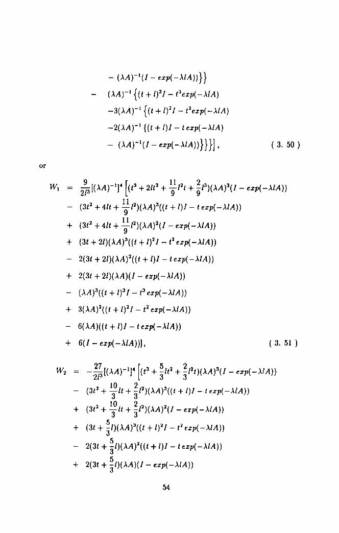
- (AArl(l- exp( -~/A»}}}] , ( 3. 50 )
WI - 2~3 [(AA)-1]4 [(t3 + 2lt2 + 191/2t + ~/3)(~A)3(1 - exp( -~/A»
- (3t 2 + 4lt + 191/2)(~A)3«t + 1)1 - t exp( -~/A»
+ (3t 2 + 4lt + 1; 12)(~A)2(1 - exp( -MA»
+ (3t + 2/)(~A)3«t + 1)21 - t'l exp( -MA»
- 2(3t + 2/)(AA)2«t + 1)/ - t exp( -~/A»
+ 2(3t + 2/)(~A)(/ - exp( -~/A»
- (AA)3«t + 1)3J - t3exp(-~/A»
+ 3(~A)'l«t + 1)2 J - t2 exp( -~/A»
- 6(~A)(t + I)J - t exp( -~/A»
+ 6(/ - exp( -AlA»], ( 3. 51 )
W2 = - ~~[(AA)-1]4 [(t3 + ~lt'l + ~/2t)(~A)3(1_ exp(-~IA» 10 2
- (3t 2 + :fit + 3/2)(~A)3«t + 1)/ - t exp( -~/A»
10 2 + (3t 2 + :fit + 3/2)(~A)2(1- exp( -~/A»
+ (3t + ~/)(~A)3«t + I)'lJ - t:l cxp( -~IA» 5
- 2(3t + 31)(~A)2«t + 1)/ - t exp( -~IA»
5 + 2(3t + 3/)(~A)(I- exp( -~/A»
54
- (,xA)3((t + 1)3/_ t3exp(-,xIA))
+ 3(,xA)2((t + 1)2/ - t2 exp( -,xIA))
- 6(,xA)((t + 1)/ - t exp( -,xIA))
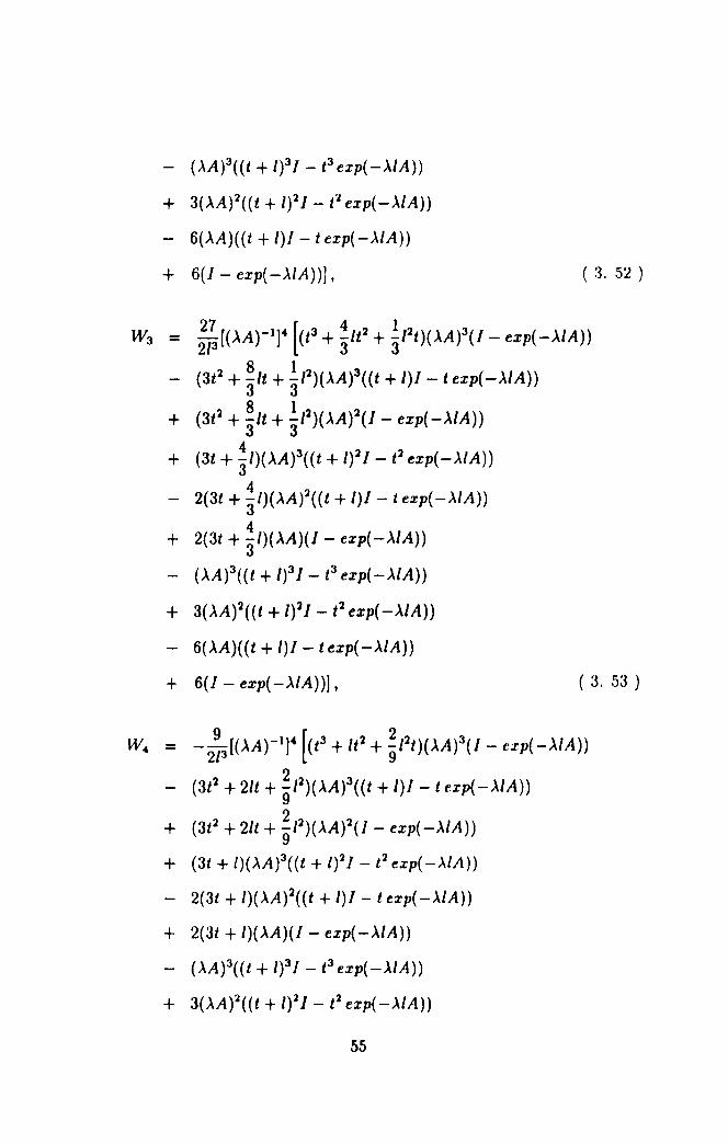
+ 6(/ - exp( -,xIA))] , ( 3. 52 )
W3 = ~/~ [(,xAtl]4 [(t3 + ~1t2 + ~rlt)(,xA)3(1- exp( -,xIA))
8 1 - (3t2 + 31t + 3/2)(,xA)3((t + 1)/ - t exp( -,xIA))
8 1 + (3t2 + 31t + 3/2)('\A)2(I - exp( -'\IA))
+ (3t + ~/)('\A)3((t + 1)2/ - t2 exp( -'\IA))
4 - 2(3t + a/)(,xA)2((t + 1)/ - t exp( -,xIA))
4 + 2(3t + 3/)(,xA)(I - exp(-,xIA))
_ (AA)3((t + 1)3/ - t3 exp( -'\IA))
+ 3('\A)2((t + 1)2/ - t2 exp( -'\IA))
- 6('\A)((t + 1)/- texp(-MA))
+ 6(1 - exp( -'\IA))), ( 3. 53 )
W4 = - 2~3[(AA)-l]4 [(t3 + /t 2 + ~/2t)('\A)3(J - exp( -'\IA))
2 - (3t2 + 21t + g/2)('\A)3((t + 1)/ - t exp( -'\IA))
+ (3t2 + 21t + ~/2)('\A)2(J - exp( -,xIA))
+ (3t + 1)(,xA)3((t + 1)2/ - t 2 exp( -,xIA))
- 2(3t + 1)(,xA)2((t + 1)/ - t eXIJ( -'\IA))
+ 2(3t + I)('\A)(/ - exp( -MA))
- (,xA)3((t + 1)3/ - t3exp(-.\IA))
+ 3(,xA)2((t + 1)2/_ t2 exp( -,xIA))
55

- 6('\A)((t + 1)1 - 1 exp( -AlA)
+ 6(1 - exp( -'\IA)].
Simplification gives
( 3. 54 )
WI = _(PA)-l),' t3 + 2/t' + -/'t + _/3 - (I + 1)(31' + 41t + _I') 9 [{ 11 2 11
2J3 9 9 9
+ (3t + 2/)(t + I)' - (t + 1)3} ('\A)3
+ {3t' + 4lt + 191/2 - 2(3t + 2/)(t + I) + 3(t + I)'} ('\A)'
+ {2(3t + 2/) - 6(t + I)} ('\A) + 61
+ {{ _(t3 + 2lt' + 1; (It + ~/3) + t(3t2 + 41t + 191/,)
- (3t + 2/)t2 + t3} PA)3
+ {-(3t 2 + 41t + 191/,) + 2t(3t + 2/) - 3t:l} ('\A):l
+ {-2(3t + 2/) + 6t)} ('\A) - 61} exp( -'\A)] , ( 3. 55 )
W2 = -_(PA)-1)4 t3 + _It' + -/'t - (t + 1)(3t' + -It + _I') 27 [{ 5 2 10 2 213 3 3 3 3
+ (3t + ~/)(t + I)' - (t + 1)3} pA)3
+ {3t2 + 1; It + ~/' _ 2(3t + ~/)(t + I) + 3(t + I)'} PA)'
+ {2(3t + ~/) - 6(t + I)} ('\A) + 61
+ {{ _(t3 + ~It' + ~/:lt) + t(3t' + 1; It + ~/:l)
- (3t + ~/)t2 + t3} pA)3
+ {-(3t 2 + 13° It + ~/') + 2t(3t + ~/) - 3t2} ('\A)'
+ {-2(3t + ~/) + 6t)} ('\A) - 61} tXp( -.\A)] , ( 3. 56 )
W3 _ ~(('\A)-1)4 [{t3 + ~/t' + !/2t - (t + 1)(3t' + ~It + !/') 2/3 3 3 3 3
+ (3t + ~I)(t + I)' - (t + 1)3} ('xA)3
56

+ {3t2 + ~tt + ~/2 - 2(3t + ~/)(t + l) + 3(t + 1)2} (..\A)2 333
+ {2(3t + ~/) - 6(t + l) } (..\A) + 61
{{ 4 1 8 1 + _(t3 + 3 lt2 + 3 /2t ) + t(3t2 + 3ft + 3/2)
- (3t + ~/)t2 + t3} (AA)3
+ {-(3t 2 + ~lt + ~/2) + 2t(3t + ~/) - 3t2} (AA)2
+ {-2(3t + ~/) + 6t)} (AA) - 61} exp( -AA)] , ( 3. 57 )
W4 = -~«,xA)-1)4 [{t3 + /t 2 + ~/2t - (t + 1)(3t2 + 2lt + ~rl) 2[3 9 9
+ (3t + I)(t + I? - (t + 1)3} (AA)3
+ {3t2 + 2lt + ~/2 - 2(3t + I)(t + I) + 3(t + 1)2} (AA)2
+ {2(3t + I) - 6(t + In (AA) + 61
+ {{ _(t3 + tt2 + ~/2t) + t(3t2 + 21t + ~/2) - (3t + l)t2 + t3} (AA)3
+ {-(3t 2 + 21t + ~/2) + 21(31 + I) - 3{1} (AA)2
+ {-2(3t + I) + 6t)} (AA) - 61} exp( -AA)].
Then it is easy to show that
WI - 2~3 [(,xA)-1)4 { 61 - 2AIA + ~(AIA)2
( 3. 58 )
- (61 + 4 AlA + 1: (AIA)2 + ~(AIA)3) exp( -ALA)} ,( 3. 59 )
W2 - - ~~ [(AA)-1]4 {61 - ~AIA + ~(..\IAf'
- (61 + 13° AlA + ~(AIA)2) exp( -AlA) } , ( 3. 60 )
W3 = 27 [(AAfl)4 {61 - ~AIA + ~(AIA)2 2[3 3 3
- (61 + ~AIA + ~(AlA)2) exp( -AlA)} , ( 3. 61 )
57
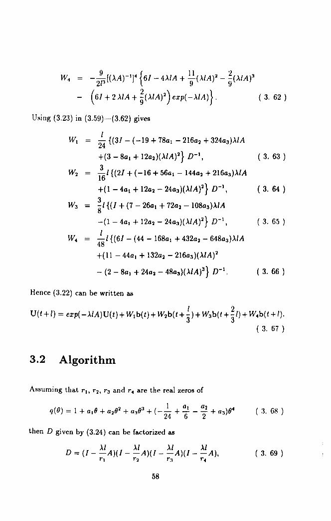
W.. = -~[(AA)-II'. {61 - 4AIA + .!..!.(AIA)l - ~(A1A)3 2P 9 9
- (61 + 2 ALA + ~(AIA)l) exp( -ALA)} . ( 3. 62 )
Using (3.23) in (3.59)-(3.62) gives
I WI = 24 {(31 - (-19 + 78al - 216a2 + 324a3)AIA
+(3 - 8a1 + 12a2)(AIA)2} D- I, ( 3. 63 )
3 W2 = 161 {(21 + (-16 + 56al - 144a2 + 216a3)AIA
+(1 - 4a1 + 12a2 - 24a3)(AIA)2} D-1, ( 3. 64 ) 3
W3 = 81 {(I + (7 - 26a1 + 72a2 - 108a3)AIA
-(1 - 4al + 12a2 - 24a3)(AIA)2} D- 1, ( 3. 6.5 )
I W" - 481 {(61 - (44 - 168al + 432a2 - 648a3)AIA
+( 11 - 44al + 132a2 - 216a3)(AlAf"
- (2 - 8al + 24a2 - 48a3)(AIA)3} D- I. ( 3. 66 )
Hence (3.22) can be written as
I 2 U(t + /) = exp( -AlA)U(t) + WI b(t) + W2b(t + 3) + W3b(t + 3/) + W"b(t + I).
( 3. 67 )
3.2 Algorithm
Assuming that rlt r2, r3 and r" are the real zeros of
( :~. 68 )
then D given by (3.24) can be factorized as
AI AI Al AI D = (J - -A)(I - -A)(1 - -A)(I - -A),
rl rl r3 r4 ( 3. 69 )
58
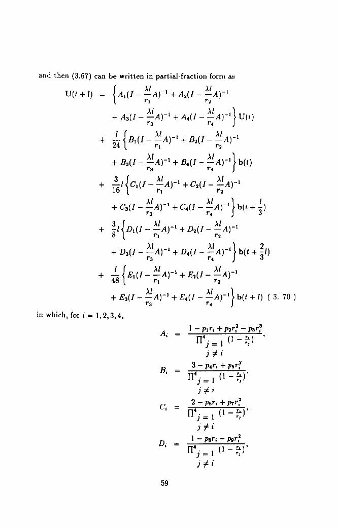
in which, for i = 1,2,3,4,
59
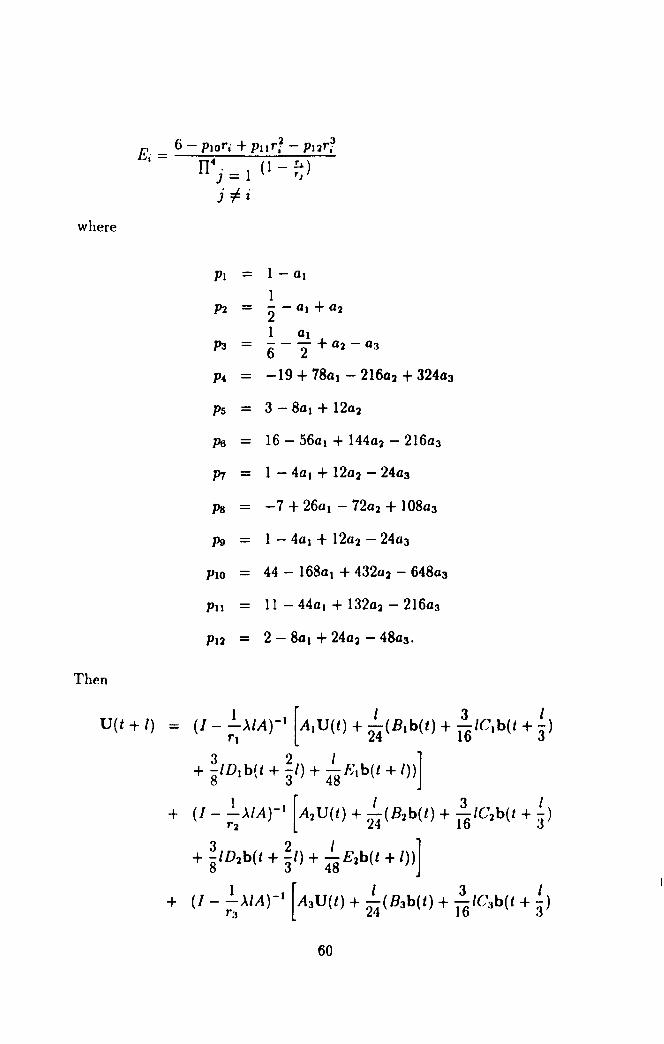
2 3
Ej = 6 - PlOr, + Pl1 r, - pur,
n4 . (1 - ~) } = 1 r J
j#i
where
PI = 1 - al
1 1'2 - - - at + a2
2 1 al
1'3 = - - - + a2 - a3 6 2
P4 = -19 + 78al - 216a2 + 324a3
ps = 3 - 8al + 12a2
1'6 - 16 - 56al + 144a2 - 216a3
P7 - 1 - 4al + 12a2 - 24a3
Ps = -7 + 26al - 72a2 + 108a3
pg = 1 - 4al + 12a2 - 24a3
PIO = 44 - 168al + 432a2 - 648a3
Pll = 11 - 44al + 132a2 - 216a3
P12 = 2 - 8al + 24a2 - 48a3.
Then
60
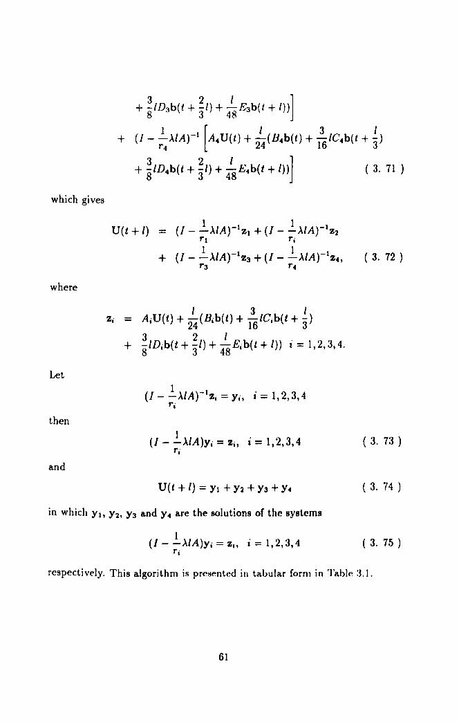
which gives
where
Let
then
and
U(t + /)
(1- .!.A1AtlZi = Yi, i = 1,2,3,4 ri
1 (1- -~IA)yj = Zi, i = 1,2,3,4
rj
U(t + /) = Yl + Y:z + Y3 + Y.
in which y., Y:z, Y3 and Y. a.re the solutions of the systems
(l - .!.A1A)Yi = Zi, i = 1,2,3,4 ri
( 3. 72 )
( 3. 73 )
( 3. 74 )
( 3. 75 )
respectively. This algorithm is presented in tabular form in 'I'abl(· ~J.l.
61

3.3 Numerical Examples
In this section a representative of many other methods ba.'ied on (:3.23) will
be used. So taking
and
64 at =-
25 1
al = -3
547 a3 = 600
Taj and Twizell [39], which give a small local trunction error, it is found that
rt =-0.931580908085238, rl=-1.81471985800593, r3=-2.00000000000000, r .. =-2.26051914612921
are the real zeros of (3.24). These values produce
Al = 0.211455566708523, A3= 108.000000000009, B t = -92.8251781314359, B3=-81O.000000000074, Ct = 68.1850562154185, C3 =972.000000000081, D t = -37.3634484931130, D3=-486.000000000044 , Et = 255.352513419023, E3 =4212.00000000038,
3.3.1 Example 1
A 2= -53.3503067445635, A .. = -53.8611488221542, B 2= 164.030220881621, B .. = 141.194951249882, C2=-160.226330382964 , C .. =-217.958125892541, D l = 399.961234456115, D .. = 124.402214036502, E l =-:3296.46069786R71 , E .. =-1164.89181555069
Consider the one space variable partial differential equation
au au at+ax=O' O<x<l, t>O.
62
( 3. 76 )

subject to the boundary conditions
u(O, t) = -sin(2k7rt), t > 0, ( 3. 77 )
where k is a positive integer and the initial condition
u(x,O) = sin(2k7rx), 0 ~ x $ 1. ( 3. 78 )
This problem has theoretical solution
u(x, t) = sin[2k1l'"(x - i)] ( 3. 79 )
(see Oliger [31)). The integer k gives the number oC complete waves in the
interval 0 $ x ~ 1. Using the Algorithm 1 with the inCormation given at the
beginning of this section the problem ({3. 76)-(3. 78)} is solved Cor h = 6!0 and I = io so that r = 8.0(r = *), using k = 2 and 4 and compared with
the results obtained by Arigu et al. [5] whose method requires the use of
complex arithmatic. The numerical solutions Cor k = 2 and k = 4 at time
t = 1.0 and t=1O.0 respectively are depicted in Figure 3.1 and Figure 3.2.
In these experiments the method behaves smoothly over the whole interval
o $ x $ 1 and no oscillations are observed. Maximum errors at time t=O .. '),
1.0, 2.0, 4.0, 10.0, are given in Table 3.2.
3.3.2 Example 2
Consider again the one space variable partial differential equation (3.2)
au au at + ax = 0, 0 < x < 1, t > O. ( :J. 80 )
subject to the boundary conditions
u(O,t) = e-', t > 0, ( 3. 81 )
63
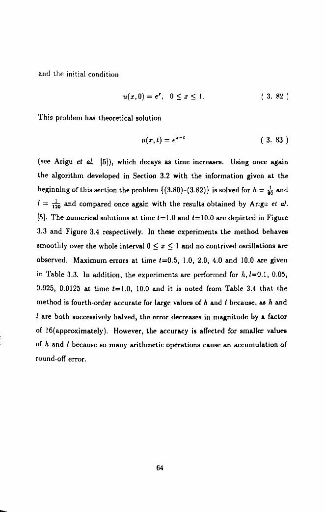
and the initial condition
( 3. 82 )
This problem has theoretical solution
u(x, t) = ez - I ( 3. 83 )
(see Arigu et al. [5]), which decays as time increases. Using once again
the algorithm developed in Section 3.2 with the information given at the
beginning of this section the problem {(3.80)-(3.82)} is solved for h = 810 and
I = l~O and compared once again with the results obtained by Arigu et al.
[5]. The numerical solutions at time t=1.0 and t=IO.0 are depicted in Figure
3.3 and Figure 3.4 respectively. In these experiments the method behaves
smoothly over the whole interval 0 ~ x ~ 1 and no contrived osciJIations are
observed. Maximum errors at time t=0.5, 1.0, 2.0, 4.0 and 10.0 are given
in Table 3.3. In addition, the experiments are performed for h, 1=0.1, 0.05,
0.025, 0.0125 at time t=1.0, 10.0 and it is noted from Table 3.4 that the
method is fourth-order accurate for large values of h and I because, as h and
I are both successively halved, the error decreases in magnitude by a factor
of 16(approximately). However, the accuracy ill affected for smaller values
of h and I because so many arithmetic operations cause a.1I accumulation of
round-off error.
64

Table 3.1: Algorithm 1
Steps Processor 1 Processor 2 Processor 3 Processor 4
1 I, rh V o, A, Al I, r2, V o, A, A2 I, r3. V o, A. A3 I. r ... VOl A, A .. Input BI.CI,DI.EI B2• C2, D2 , E2 B3• C3, D3• E3 B ... C ... D ... E ..
2 Comp 1- ~'A
rl 1- ).,/A
r, 1- ).,/A
r3 1- ~, A
r.
3 1- ~'A 1- ~I A I - ,\1 A I - ,\1 A rl r, r3 r.
Decom = LlUl = L2U2 = L3U3 = L .. U ..
4 b I = b(t) bl = b(t) bI = b(t) bl = b(t) b2 = b(t + 1) b2 = b(t + i)
Comp b3 = b(t + ¥) b3 = b(t + -t) b1 = b(t + ~} b3 = b(t + :f}
b:l = b(t + i) b3 = b(t + ~)
b .. = b(t + I) b .. = b(t + I) b .. = b(t + I) b .. = b(t + I)
5 WI(t) Wl(t) W3(t) w .. (t) Using = "'8 {2B l b l = "'8 {2B2b I = .. ~ {2B3 b l = 18 {2B .. b l
+9CI b2 +9C2bl +9C3 b1 +9C.lb2
+18Dlb3 +18D2b3 +18D3 b3 +18D .. b3
+ Elb .. } + Elb .. } + E3b .. } +E .. b .. }
6 LIUlYI(t) L2U2Y2(t} L3U3Y3(t} L .. U .. y .. (t) Solve = AIU(t) = AlV(t) = A3U (t) = A .. U(t)
+Wl (t) +W2(t} +W3(t) +w .. (t}
7 U(t + l) = ydt) + Y2(t) + Y:I(t) + y .. (t}
8 GO TO Step 4 for next time step I
65
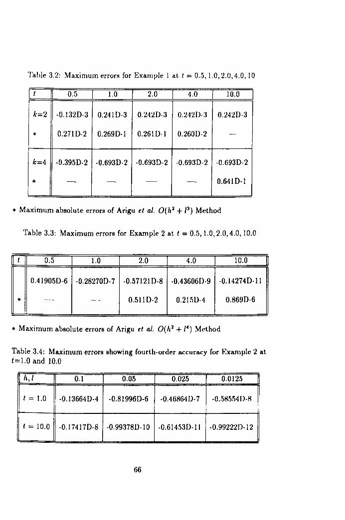
Table 3.2: Maximum errors for Example 1 at t = 0.5,1.0,2.0,4.0,10
I t II 0.5 1.0 2.0 4.0 10.0
k=2 -0.1320-3 0.2410-3 0.242D-3 0.2420-:1 0.2420-3
* 0.2710-2 0.2690-1 0.2610-1 0.2600-2 --~
k=4 -0.3950-2 -0.693D-2 -0.693D-2 -0.693D-2 -0.693D-2
* - - - - 0.6410-1
* Maximum absolute errors of Arigu et al. O(h'l + 13) Method
Table 3.3: Maximum errors for Example 2 at t = 0.5,1.0,2.0,4.0,10.0
II t II 0.5 1.0 2.0 4.0 10.0
0.419050-6 -0.282700-7 -0.571210-8 -0.436060-9 -0.142740-11
* -- -- 0.5110-2 0.2150-4 0.8690-6
• Maximum absolute errors of Arigu d al. O(h2 + 1") Method
Table 3.4: Maximum errors showing fourth-order accuracy for Example 2 at t=l.O and 10.0
h, I 0.1 0.05 0.025 0.0125
t = 1.0 -0.13664 0-4 -0.819960-6 -0.46864 D- 7 -0 .. 1)85.',)4 D-8 I
I;
t = 10.0 -0.174170-8 -0.99378D-10 -0.614530-11 -0.99222D-12
66
II

1
0.8
0.6 -0.4
0.2 ~:
~ 0-
-0.2,",
-0.4
-0.6
-O.8~
-1 0
Figure 3.1
I
.
I
100 200 300 400 500 600 Space Steps
Figure 3.1: Numerical solution of example 1 for k = 2, h = ts!o and I = 'io at time t=O.5
67
-
-
-
-
-
-
700

:;)
Figure 3.2 1r-~---.------__ ----__ ~ __ ~~,-______ ~~ ____ .-____ -. ..
0.8
0.6
0.4
-0.2
-0.4
-0.6
-0.8
-1 0
I
.. 100 200 300 400 500 600
Space Steps
Figure 3.2: N umerica.l solution of example 1 for k = 4, h = e!o and I = io at time t=10.0
68
l
.., i
I
700

Figure 3.3 1r------.�------~------T_I-----,,-------r------T,------~----~
0.9f- -
0.8~ .
-
0.6 r-
0.5~ . I
I
0.4 f- -
0.3~----~------~----~------~~------~----~~------~----~ o 10 20 30 40 50 60 70 Space Steps
Figure 3.3: Numerical solution of example 2 for h = io and I = 1~ at time t=1.0
69
80

13 Figure 3.4
, 1 , , ,
12 r- .. -
11 r- -
10 -
9f- . ::l
8f- -
7f-
Sf-
5f- -
4 i I i
0 10 20 30 40 50 60 70 80 Space Steps
Figure 3.4: Numerical solution of example 2 for h = 8~ and I = 1;0 at time t=1O.0
70

Chapter 4
Third-Order Methods for the Advection-Diffusion Equation
4.1 The Model Problem
A typical problem in applied mathematics is the advection-diffusion equation.
This initial/ boundary-value problem (IBVP) is given by
au(x, t) + au(x, t) _ aa2u f( t) at a ax - tJ ax2 + x, , a,/3 > 0, 0 < x < X, t > 0
with the boundary conditions
and the initial condition
u(O, t) - h1(t), t> 0
u(X, t) - h2(t), t > 0
u(x,O)=g(x), O~x~X
(4. 1 )
( 4. 2 )
( 4. 3 )
( 4. 4 )
where g(x) is a given continuous function of x and h1(t), h2(t) are given
continuous functions of t.
71
, ' f I L '
, I I,

4.2 The Method
Dividing the interval [0, X] into N + 1 subintervals each of width h, so that
(N + l)h = X, and the time variable t into time steps each of length I gives
a rectangular mesh of points with co-ordinates
(m = 0,1,2, ... ,N + 1 and n = 0,1,2, ... ) covering the region R = [0 < x <
X] x [t > 0] and its boundary 8R consisting of the lines x = 0, x = X and
t = 0.
To approximate the first-order space deri vati ve in (4.1) to third -order
accuracy at some general point (x, t) of the mesh, assume that it may be
replaced by the four-point formula
8u(x, t) 8x - *{au(x-h,t)+bu(x,t)+CU(X+h,t)
+ du(x + 2h, tn. ( 4. 5 )
Expanding the terms u(x - h, t), u(x + h, t) and u(x + 2h, t) as Taylor series
about (x, t) in (4.5) gives
h 8u(x,t) _ (a+b+c+d)u(x,t) 8x
( 2d) h8u(x, t)
+ -a+c+ 8x
+ ~( 4d) h282u(x, t) 2! a + c+ 8x2
+ ~(_ 8d)h3lJ3U(x,t) 3! a + c+ 8x3
+ ~( 16d) h4 tru(x, t) 4! a+c+ 8x"
+ O(h") as h ~ O.
72
( 4. 6 )
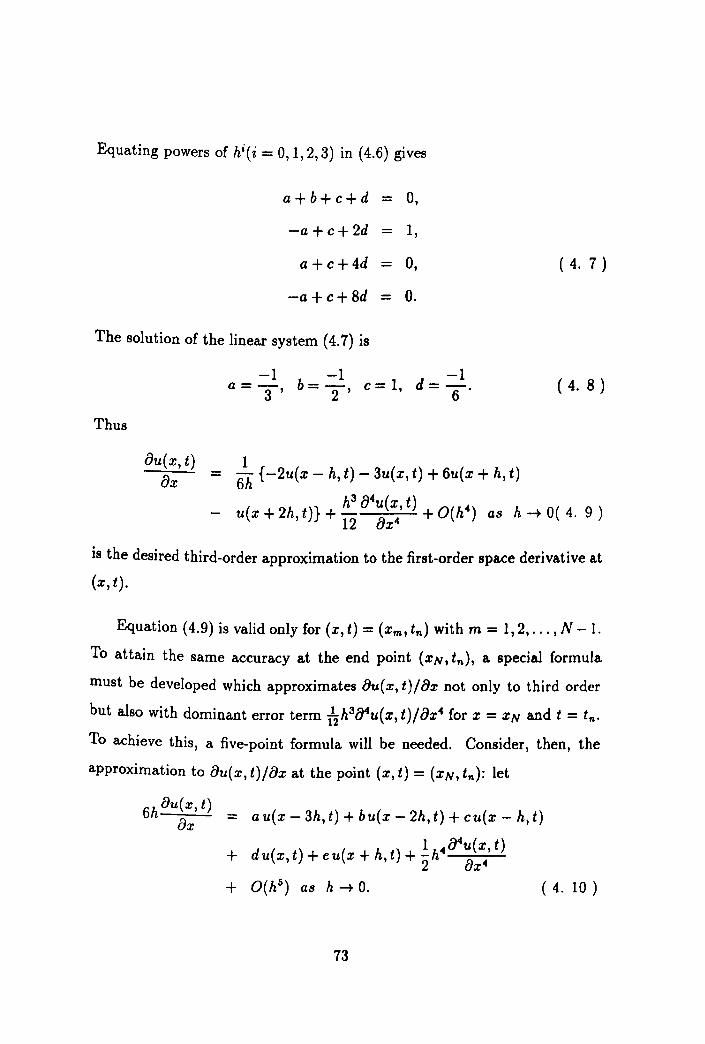
Equating powers of hi(i = 0,1,2,3) in (4.6) gives
a + b+ c+ d - 0,
-a+c+2d - 1,
a + c+ 4d - 0,
-a +c+8d - O.
The solution of the linear system (4.7) is
Thus
8u(x, t) 8x
-1 -1 -1 a = 3' b = 2' c = 1, d = T'
1 - 6h {-2u(x - h, t) - 3u(x, t) + 6u(x + h, t)
( 4. 7 )
( 4. 8 )
h3 84u(x t) u(x + 2h, tn + 12 8X4' + O(h4) as h ~ O( 4. 9 )
is the desired third-order approximation to the first-order space derivative at
(x, t).
Equation (4.9) is valid only for (x, t) = (xm' tn) with m = 1,2, ... ,N - 1.
To attain the same accuracy at the end point (XN' tn), a special formula
must be developed which approximates 8u(x, t)/8x not only to third order
but also with dominant error term 112h3B4u(x, t)/8x4 for x = XN and t = tn.
To achieve this, a five-point formula will be needed. Consider, then, the
approximation to 8u(x, t)/8x at the point (x, t) = (XN' t n ): let
6h 8u(x, t) 8x - a u(x - 3h, t) + bu(x - 2h, t) + cu(x - h, t)
1 4B4U(X,t) + du(x,t)+eu(x+h,t)+2"h 8x4
+ O(h5) as h ~ O. ( 4. 10 )
73
Then expanding the terms u(x - 3h, t), u(x - 2h, t), u(x - h, t) and u(x + h, t)
as Taylor series about the point (x, t) gives
6hou
(x,t) (a+b+c+d+e)u(x,t) ox
au(x, t) + ( -3a - 2b - c + e) h ax
1 a2u(x t) + ,(9a++4b+c+e)h2 a 2' 2. x
1 ) 3l)3U(X,t) + - ( -27 a - 8b - c + e h -..,~....:.. 3! ax3
+ ~(81a + +16b + c + e - 12) h404ua(:, t) 4. x
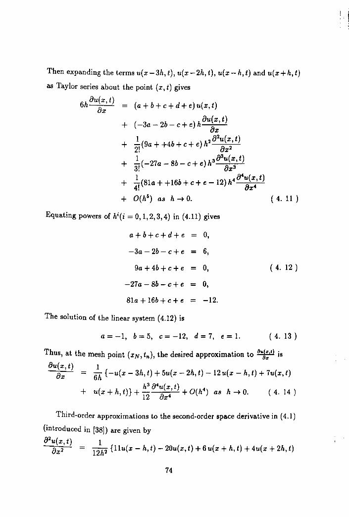
+ O( h5) as h ~ O. ( 4. 11 )
Equating powers of hi(i = 0,1,2,3,4) in (4.11) gives
a+b+c+d+e - 0,
-3a - 2b - c+ e - 6,
9a + 4b+ c+ e - 0, ( 4. 12 )
-27a - 8b - c + e - 0,
81a + 16b + c + e - -12.
The solution of the linear system (4.12) is
a=-1, b=5, c=-12, d=7, e=l. ( 4. 13 )
Thus, at the mesh point (XN, tn), the desired approximation to ovJ:") is
ou(x, t) 1 ox - 6h {-u(x - 3h, t) + 5u(x - 2h, t) - 12 u(x - h, t) + 7u(x, t)
h3 04u(x t) + u(x + h, in + 12 ox4' + O(h4) as h ~ O. ( 4. 14 )
Third-order approximations to the second-order space derivative in (4.1)
(introduced in [38]) are given by
02U(x, t) 1 OX2 = 12h2 {l1u(x - h, t) - 20u(x, t) + 6 u(x + h, t) + 4u(x + 2h, t)
74

- u(x + 3h, tn + h3 8S~(~, t) + O(h4) as h -+ O.
12 x ( 4. 15 )
for (x,t) = (xm,tn ), m = 1,2, ... ,N - 2,
82u(x, t) 1 8x2 - 12h2 {u(x - 3h, t) - 6u(x - 2h, t) + 26 u(x - h, t)
- 40u(x, t) + 21u(x + h, t) - 2u(x + 2h, tn
h3
8Su(x, t) O(h4) as h -+ O.
+ 12 8xs + ( 4. 16 )
for (x, t) = (XN-b tn) and
82u(x,t) 1 8x2 = 12h2 {2u(x - 4h, t) - llu(x - 3h, t) + 24 u(x - 2h, t)
- 14u(x - h, t) - 10u(x, t) + 9u(x + h, tn + h
3 8
Su(x, t) + O(h4) as h -+ O.
12 8xs
for (x, t) = (XN, tn).
( 4. 17 )
Applying (4.1)-(4.4) with (4.9), (4.14), (4.15), (4.16) and (4.17) as ap
propriate to the N mesh points of the grid at time level t = tn leads to the
system of first-order ordinary differential equations given in vector-matrix
form as
~;t) = AU(t) + bet), t > 0
with initial distribution
U(O) = g,
where
( 4. 18 )
( 4. 19 )
U(t) = [U1(t), ... , UN(t)V, 1
bet) = [!t(t) + 12h2 (4ah + ll,O)hl(t), ll(t), 13(t), ... , IN-3(t),
{3 1 IN-2(t) - 12h2h2(t),IN-l(t) + 12h2(2ah - 2{3)h2(t),
1 IN(t) + 12h2 (-2ah + 9{3)h2(t)V,
g = [g(Xl),g(X2), .. ' ,9(XN)]T,
75
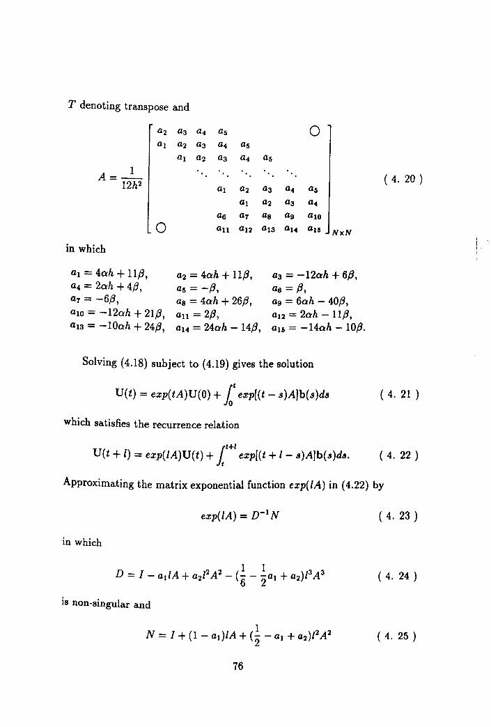
T denoting transpose and
1 A=-
12h2
in which
al = 4a:h + 11,8, a4 = 2ah + 4{3, a1 = -6,8,
a2 al
0
alO = -12ah + 21,8, al3 = -10a:h + 24,8,
a3 a4 as a2 a3 a4 as al a2 a3 a4
al a2 al
a6 a1 all al2
a2 = 4ah + 11,8, as = -(3, as = 4a:h + 26{3, an = 2{3, al4 = 24ah - 14,8,
0
as
a3 a4 as a2 a3 a4 as a9 alO al3 al4 au NxN
a3 = -12a:h + 6{3, a6 =,8, a9 = 6a:h - 40,8, al2 = 2ah - 11,8, au = -14a:h - 10{3.
Solving (4.18) subject to (4.19) gives the solution
U(t) = exp(tA)U(O) + fot exp[(t - s)A]b(s)ds
which satisfies the recurrence relation
{HI U(t + I) = exp(IA)U(t) + Jt exp[(t + /- s)A]b(s)ds.
( 4. 20 )
( 4. 21 )
( 4. 22 )
Approximating the matrix exponential function exp(lA) in (4.22) by
exp(lA) = D- I N ( 4. 23 )
in which
D 22 (1 1 )33 = I - aliA + a21 A - - - -at + a2 I A 6 2
( 4. 24 )
is non-singular and
( 4. 25 )
76
, I I.

as in Chapter 2 and the integral term by
rt+1
it exp((t + 1- s)A)b(s)ds = Wlb(sl) + W2b(S2) + W3b(S3) (4. 26 )
where SI =f S2 =f S3 and WI, W 2 and W3 are matrices.
These matrices can be obtained by putting" = -1 in (2.53)-(2.55) giving
I _ WI = '6{(I + (4 - gal + 12a2)IA} D I, ( 4. 27 )
W. 21{ } 1 () 2 - 3" (I - (1 - 3al + 6a2)IA D- , 4. 28
W3 = f{(I + (3 - 9al + 12a2)lA + (1 - 3al + 6a2)/2 A2} D-1•
( 4. 29 )
Hence (4.22) can be written as
1 U(t + I) = exp(lA)U(t) + Wlb(t) + W2b(t + 2) + W3b(t + I). (4. 30 )
4.3 Algorithm
The algorithm is very similar to that given in Section 2.4 of Chapter 2 but
it is included in the interests of completeness.
Assuming that rl, r2 and r3 are the real zeros of
( 4. 31 )
then D given by (4.24) can be factorized as
I I I D = (I - -A)(I - -A)(I - -A)
rl r2 r3 ( 4. 32 )
and then (4.54) can be written in partial fraction form as
U(t + I) = {Cll (I - ~A)-I + c12(I - ~A)-l + CI3(I _ -\l A)-I} U(t) rl r2 r3
77

1 {( 1 I ( I) I I I} + -6 C21 1- -A)- + C22 I - -A - + C23(i- -A)- bet) rl r2 r3
21 { 1 I I I II} 1 + -3 C31(i- -At + C32(i- -At + c33(I - -A)- bet + -2) rl r2 r3
I { 1 1 I I I I} + - C41(I - -At + c42(I - -At + C43(I - -At bet + l) 6 ~ ~ ~
( 4. 33 )
where
j = 1,2,3,
i = 1,2,3
and
C . = 1 + (3 - gal + 12a2)rj + (1 - 3al + 6a2)rJ 4) n3. (1 _ !J.) ,
1=1 r,
i = 1,2,3.
i:f:i So that
U(t + I) - All{cu U(t) + ~(C2Ib(t) + 4c3l b(t + ~) + C4l b(t + I))}
+ A;I{CI2U(t) + ~(C22b(t) + 4C32b(t + ~) + C42b(t + I))}
where
l{ 1 I } + A3" C13U (t) + 6(C23b(t) + 4C33b(t + 2') + C43b(t + I)) ,
1 Ai = I - - A, i = 1, 2, 3,
ri
78
( 4. 34 )
( 4. 35 )

or
where
Let
then
3
U(t + I) = E A;lZi ;=1
A- 1z - y' i i - •
in which yt, Y2 and Y3 are the solutions of the systems
AiYi = Z;, i = 1,2,3.
( 4. 36 )
( 4. 37 )
( 4. 38 )
respectively. This algorithm is presented in tabular form in Table 4.1.
4.4 Numerical Example
In this section only a representative of many other methods based on (4.23)
will be used. So taking
and
as in chapter 2, gives
65431 at = 50000
171151 a2 = 300000'
r1 = 2.18837132239026, r2 = 2.33987492247039, r3 = 2.356901393726.52
as the real zeros of (4.55). These values produce
ell = -176.185066638, C12 = 2051.11129521, C13 = -1873.92622858,
79
I .~
C21 = -224.317807049, C22 = 2358.75587416, C23 = -2133.43806711,
C31 = -19.0008161810, C32 = 326.498892802, C33 = -306.498076621,
C41 = -182.736963963, C42 = 1594.78928297, C43 = -1411.05231901
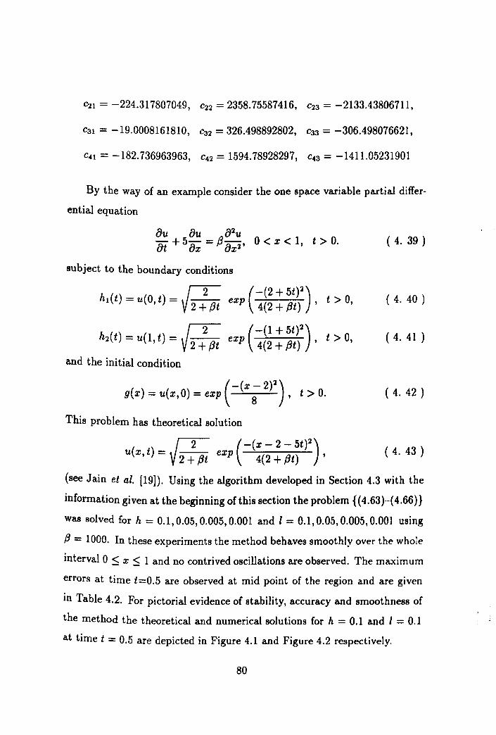
By the way of an example consider the one space variable partial differ
ential equation
au au a 2u at + 5 ax = p ax2 ' 0 < x < 1, t > O. ( 4. 39 )
subject to the boundary conditions
h (t) _ ( ) _ f2 (-(2 + 5t)2) I - u O,t - V2+7ii exp 4(2 + pt) , t > 0, ( 4. 40 )
f2 (-(1 + 5t)2) h2(t) = u(l, t) = V 2+7ii exp 4(2 + pt) ,t > 0, ( 4. 41 )
and the initial condition
g(x) = u(x,O) = exp (-(x; 2)2), t > O. ( 4. 42 )
This problem has theoretical solution
f2 (-(X - 2 - 5t)2) u(x, t) = V 2+7ii exp 4(2 + pt) , ( 4. 43 )
(see Jain et al. [19]). Using the algorithm developed in Section 4.3 with the
information given at the beginning of this section the problem {( 4.63)-( 4.66)}
was solved for h = 0.1,0.05,0.005,0.001 and I = 0.1,0.05,0.005,0.001 using
f3 = 1000. In these experiments the method behaves smoothly over the whole
interval 0 $ x $ 1 and no contrived oscillations are observed. The maximum
errors at time t=0.5 are observed at mid point of the region and are given
in Table 4.2. For pictorial evidence of stability, accuracy and smoothness of
the method the theoretical and numerical solutions for h = 0.1 and I = 0.1
at time t = 0.5 are depicted in Figure 4.1 and Figure 4.2 respectively.
80
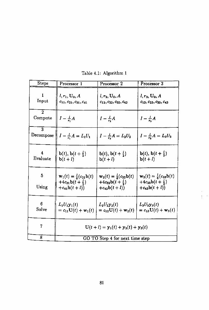
Table 4.1: Algorithm 1
Steps " Processor 1 I Processor 2 I Processor 3
1 l,rll Uo,A l,r2, U o, A I, T3, U O, A Input cu, C211 C3t, C4I CI2, C22, C32, c..2 CI3,C23,C33,c..3
2 Compute I - .LA
rl I - .LA
r2 I - .LA
r3
3 Decompose I - .LA = LIUI rl
I - .LA = L2U2 r2 I - .LA = L3U3 r,
4 b(t), b(t + 4) b(t), b(t + 4) b(t), b(t + 4) Evaluate b(t + /) b(t + /) b(t + /)
5 Wl(t) = ~(C21b(t) W2(t) = ~(C22b(t) W3(t) = HC23b(t) + 4C31 b(t + 4) +4C32b(t + 4) + 4C33b( t + 4)
Using +c41b(t + I)) +C42b(t + I)) +C43b(t + I))
6 L1U1Yl(t) L2U2Y2(t) L3U3Y3(t) Solve = Cll U(t) + Wl(t) = c12U(t) + W2(t) = C13U(t) + W3(t)
7 U(t + I) = Yl(t) + Y2(t) + Y3(t)
8 GO TO Step 4 for next time step
81
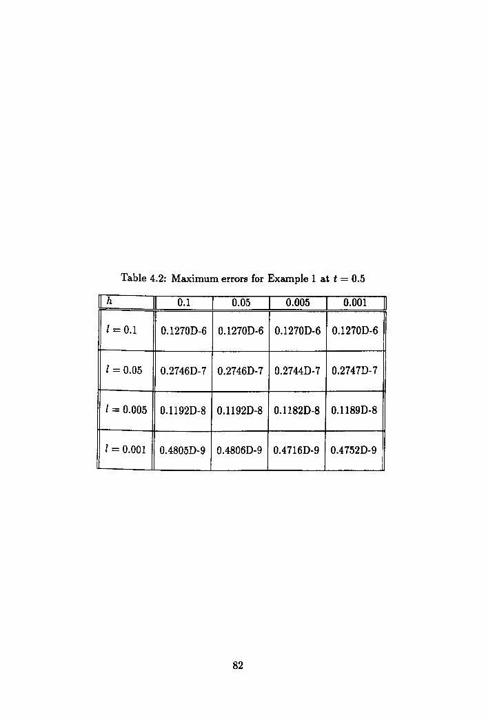
Table 4.2: Maximum errors for Example 1 at t = 0.5
II h " 0.1 0.05 0.005 0.001 "
1 = 0.1 0.1270D-6 0.1270D-6 0.1270D-6 0.1270D-6
1=0.05 0.2746D-7 0.2746D-7 0.2744D-7 0.2747D-7
1 = 0.005 0.1192D-8 0.1192D-8 0.1182D-8 0.U89D-8
1 = 0.001 0.4805D-9 0.4806D-9 0.4716D-9 0.4752D-9
82
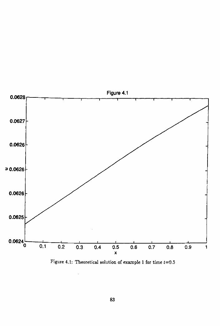
Figure 4.1 0.~28r----r----r----r----r---~---.r---'----'----.----,
0.0627
0.0626
:::J 0.0626
0.~26
0.0625
0.0624~--~--__ L-__ ~ __ ~~ __ ~ __ ~ ____ ~ __ ~ ____ ~ __ ~ o 0.1 0.2 0.3 0.4 0.5
x 0.6 0.7 0.8
Figure 4.1: Theoretical solution of example 1 for time t=O.5
83
0.9 1
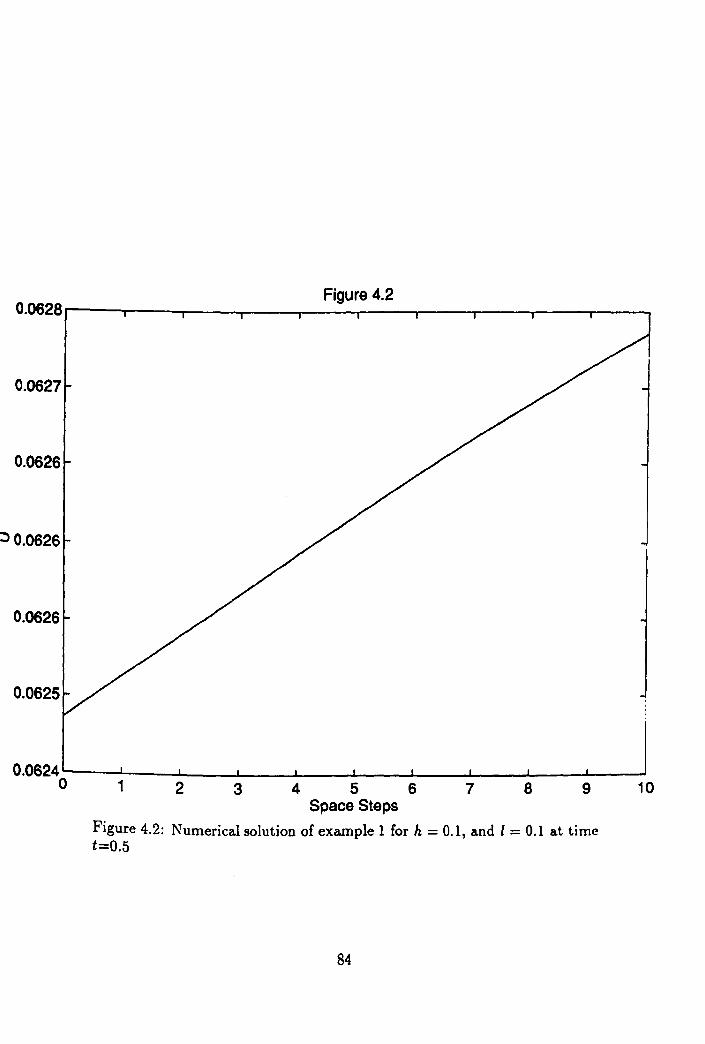
Figure 4.2 0.~28r----.----~--~--~----~--~----~--~----~--~
0.0627
0.~26
:) 0.0626
0.0626
0.0625
0.0624~--~--~ ____ ~ __ -L ____ ~ __ ~ __ ~ ____ ~ __ ~ __ ~ o 1 2 3 456
Space Steps 7 8 9
Figure 4.2: Numerical solution of example 1 for h = 0.1, and 1= 0.1 at time t=O.5
84
10

Chapter 5
Fourth-Order Numerical Methods for the Advection-Diffusion Equation
To develop fourth-order numerical methods for advection-diffusion equations
of the type (4.1) with appropriate initial and boundary conditions speci
fied, the space derivatives in the partial differential equation are replaced by
fourth-order finite-difference approximations resulting in a system of first
order ordinary differential equations the solution of which satisfies a recur
rence relation. The accuracy in time is controlled by a fourth-order approx
imation to the matrix exponential function as in Cha.pter 3.
5.1 The Method
Consider the advection-diffusion equa.tion (4.1), mentioned here for convenience ,
£..u(x,.!2 + au(x, t) _ (302u(x, t) f( t). {3 0 X 0 at 0 ax - ox2 + X, , 0, > 0, < x < , t >
( 5. 1 )
85

with the boundary conditions
u(O,t) = !t(t)} t> ° u(l, t) = h(t) , ( 5. 2 )
in which fl(t), f2(t) are given continuous functions of t and the initial con
dition
u(x,O) = g(x), ° ~ x ~ X, ( 5. 3 )
in which g(x) is a given continuous functions of x. For a positive integer
N, let h = N~l' Considering the discretization of the region R = [0 <
x < X] x [t > 0] and its boundary oR as in Section 4.2, assume that the
combination
a u(x - 2h, t) + bu(x - h, t) + cu(x, t) + du(x + h, t) + eu(x + 2h, t)
gives the fourth-order approximation to ~; at some general point (x, t) of the
mesh. Expanding the terms u(x-2h, t), u(x -h, t), u(x+h, t) and u(x+2h, t)
as Taylor series about the point (x, t) gives
a u(x - 2h, t) + bu(x - h, t) + cu(x, t) + du(x + h, t) + e u(x + 2h, t)
- (a + b + c + d + e)u(x, t) ou
+ (-2a - b + d + 2e)h-ox
1 o'lu + 2! (4a + b + d + 4e )h'l ox2
1 3 {flu + - ( -Sa - b + d + Se)h -
3! ox3
1 lru + ,(16a + b + d + 16e)h4 0 4
4. x 1 ~u
+ -( -324a - b + d + 32e)h5-
5! ox5
+ O(h6) as h ~ O. ( 5. 4 )
Equating the powers of hi(i = 0,2,3,4) in (5.4) to zero and the power of h
to 1 gives
c+d+b+e+a = 0
86
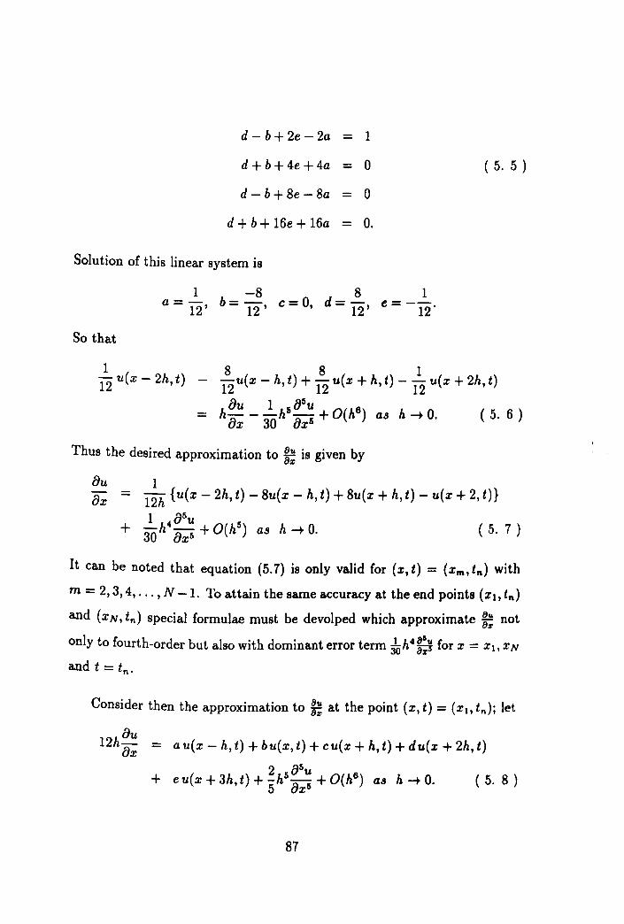
d - b + 2e - 2a - 1
d + b + 4e + 4a - 0
d - b + 8e - 8a - 0
d + b + 16e + 16a - O.
Solution of this linear system is
1 -8 8 1 a = 12' b = 12' c = 0, d = 12' e = - 12'
So that
1
( 5. 5 )
- u(x - 2h t) 12 '
8 8 1 12 u(x - h,t) + 12 u(x + h,t) - 12 u(x + 2h, t)
_ h 8u _ ~hs85U + O(h6) as h -+ O. ( 5. 6 ) 8x 30 8xs
Thus the desired approximation to ~: is given by
au 1 ax - 12h {u(x - 2h, t) - 8u(x - h, t) + 8u(x + h, t) - u(x + 2, tn
1 48su
5 (5 7) + 30 h ax5 + O( h) as h -+ O. .
It can be noted that equation (5.7) is only valid for (x, t) = (xm , tn ) with
m = 2,3,4, ... , N -1. To attain the same accuracy at the end points (XI! tn)
and (XN, tn) special formulae must be devolped which approximate ~; not
only to fourth-order but also with dominant error term ;Oh4~ for x = Xl. XN
and t = tn.
Consider then the approximation to ~; at the point (x, t) = (XlJ in); let
12h au ax - a u(x - h, t) + bu(x, t) + cu(x + h, t) + du(x + 2h, t)
( 5. 8 )
87
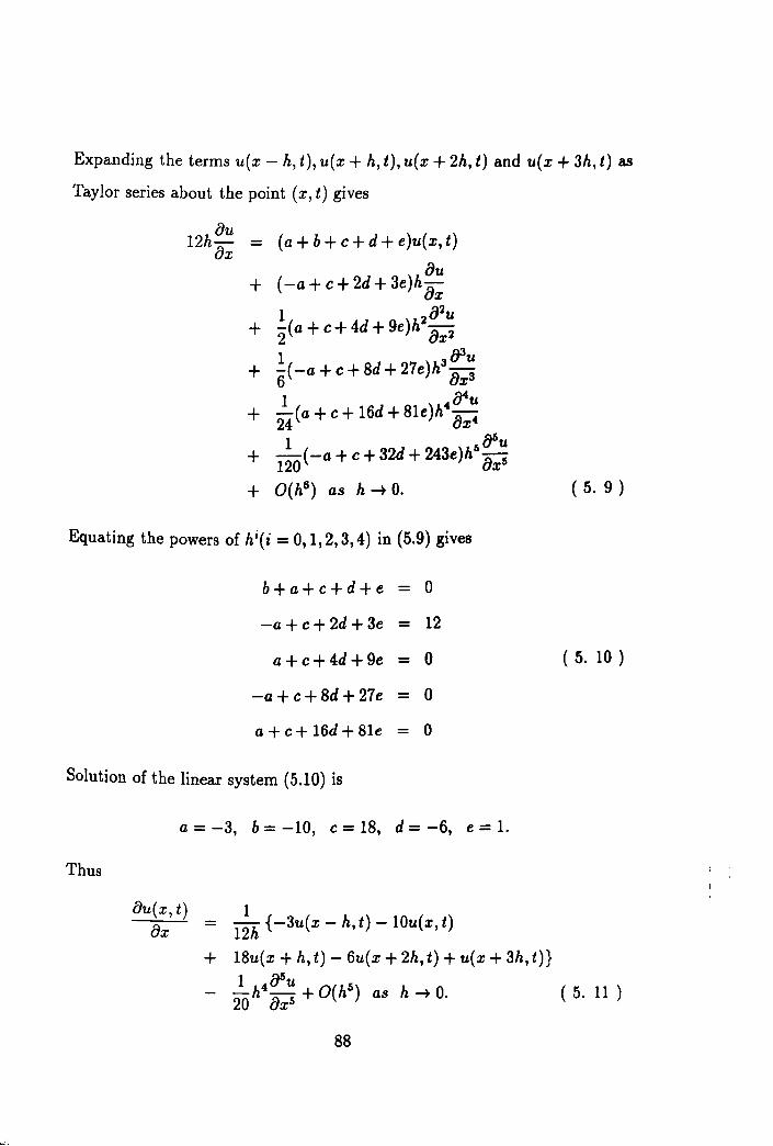
Expanding the terms u(x - h, t), u(x + h, t), u(x + 2h, t) and u(x + 3h, t) as
Taylor series about the point (x, t) gives
12hoU _ (a+b+c+d+e)u(x,t) ox
au + (-a+c+2d+3e)h
ax 1 a2u
+ -(a+c+4d+ge)h2
a 2
2 x 1 alf3u
+ -(-a+c+8d+27e)h a 3 6 x 1 • {)4u
+ 24 (a + c + 16d + 81e)h ax.
1 5a~ + 120 (-a + c + 32d + 243e)h ax5
+ O(h6) as h -+ O.
Equating the powers of hi(i = 0,1,2,3,4) in (5.9) gives
b+a+c+d+e - 0
-a+ c+ 2d +3e - 12
a +c+4d +ge - 0
-a+c+8d+27e = 0
a + c + I6d + 8Ie = 0
Solution of the linear system (5.10) is
Thus
a = -3, b = -10, c = 18, d = -6, e = 1.
ou(x, t) ox
1 - 12h {-3u(x - h, t) - 10u(x, t)
+ 18u(x + h, t) - 6u(x + 2h, t) + u(x + 3h, t)}
- ~h4a5u O(h5) as h -+ O. 20 ox5 +
88
( 5. 9 )
( 5. 10 )
( 5. 11 )

Consider, now the approximation to 8U~:.t) at the point (x, t) = (XN, tn); let
12h :: - a u(x - 3h, t) + bu(x - 2h, t) + cu(x - h, t) + du(x, t)
( 5. 12 )
Expanding the terms u(x-3h, t), u(x-2h, t), u(x- h, t) and u(x+h, t) about
the point (x, t) gives
12h:: - (a+b+c+d+e)u(x,t)
au + (-3a - 2b - c + e)h ax
1 a2u + 2(9a+4b+c+e)h2
ax2 1 3[J3u + 6 ( - 27 a - 8b - c + e) h ax3
1 tru + -(81a + 16b + c + e)h"a "
24 x 1 a"u
+ 120 (-243a - 32b - c + e)h" ax"
+ O(hB) as h -t O.
Equating the powers of hi(i = 0,1,2,3,4) in (5.13) gives
a+b+c+d+e - 0
-3a - 2b - c+ e - 12
9a + 4b+ c+ e - 0
- 27 a - 8b - c + e - 0
81a + 16b + c + e = O.
Solving the linear system (5.14) gives
a=-I, b=6, c=-18, d=10, e=3.
89
( 5. 13 )
( 5. 14 )
, I' I
I. J I •

Thus
8u(x, t) 8x
1 12h {-u(x - 3h, t) + 6u(x - 2h, t)
18u(x - h, t) + 10u(x, t) + 3u(x + h, tn 1 8su + -h4
-8
+ O(hS) as h -+ O. 20 XS
( 5. 15 )
is the desired approximation to 8uJ:,t) at the point (XN, tn).
Consider, next the fourth-order a.pproxima.tions to 83;i;,t) [39];
1 - 12h2 {-u(x - 2h, t) + 16u(x - h, t)
30u{x, t) + 16u(x + h, t) - u{x + 2h, tH 1 fJ6u 5 + -h4
-a
+ O(h) as h -+ O. 90 x6
( 5. 16 )
valid for points (x,t) = (mh,nl) m = 2,3,4, ... ,N -1,
= 121h2 {9u(x - h, t) - 9u(x, t) - 19u(x + h, t)
+ 34u(x + 2h, t) - 21u(x + 3h, t) + 7u(x + 4h, t)
1 4 EJ6u Ii) h (5 7) - u(x + 5h, tn + 90 h ax6 + O(h as -+ 0", . 1
the approximation to 82;i~,t) at the point (Xl, tn) and
- 12\2 {-u(x - 5h, t) + 7u(x - 4h, t) - 21u(x - 3h, t)
+ 34u(x - 2h, t) - 19u(x - h, t)
- 9u(x, t) + 9u(x + h, tn 1 4
asu (5) h + -h a 6 + 0 h as -+ O. 90 X ( 5. 18 )
the approximation to 82;~2,t) at the point (XN, tn).
Applying (5.1) with (5.7) or (5.11) or (5.16) or (5.17) or (5.18) as appro
priate to the N mesh points at the time level t = nl, leads to the system of
90

first-order ordina.ry differentia.l equations given by vector-matrix form as
d~?) = AU(t) + b(t), t> 0 ( 5. 19 )
with initial distribution
U(O) = g ( .5. 20 )
in which
U(t) - [UI(t), U2(t) ... , UN(t)]T, b(t) - [!t(t) + ~(9;3 + 3ah), h(t) - rks(;3 + ah), h(t), ... ,
fN-2, fN-I(t) - 12Ih2 (;3 - ah), fN(t) + 1'J~2(9f3 - 3ah)]T,
g - (g(xt} , g(X2),'" ,g(XN )]T,
T denoting transpose and
al a2 a3 a4 all as 0 as a9 alO an
1 a7 as a9 alO an
A=- ( 5. 21 ) 12h2
aT as a9 alO an a7 as a9 alO
0 a6 all a4 a3 a2 at NxN
where
al = -9;3 + lOah a2 - -19;3 - ISah a3 - 34;3 + 6ah a4 = -21;3 - ah all - 7;3 a6 - -;3 a7 - -;3 - ah as - 16{J + Sah a9 - -30;3 alO - 16;3 - Sah an - -{J + oh
Solving (5.19) subject to (5.20) gives the solution
U(t) = exp(tA)U(O) + lo' exp[(t - s)A]b(s)ds ( 5. 22 )
which satisfies the recurrence relation
{HI U(t + I) = exp(1A)U(t) + 1, exp[(t + 1 - s)A]b(s)ds. ( 5. 23 )
91
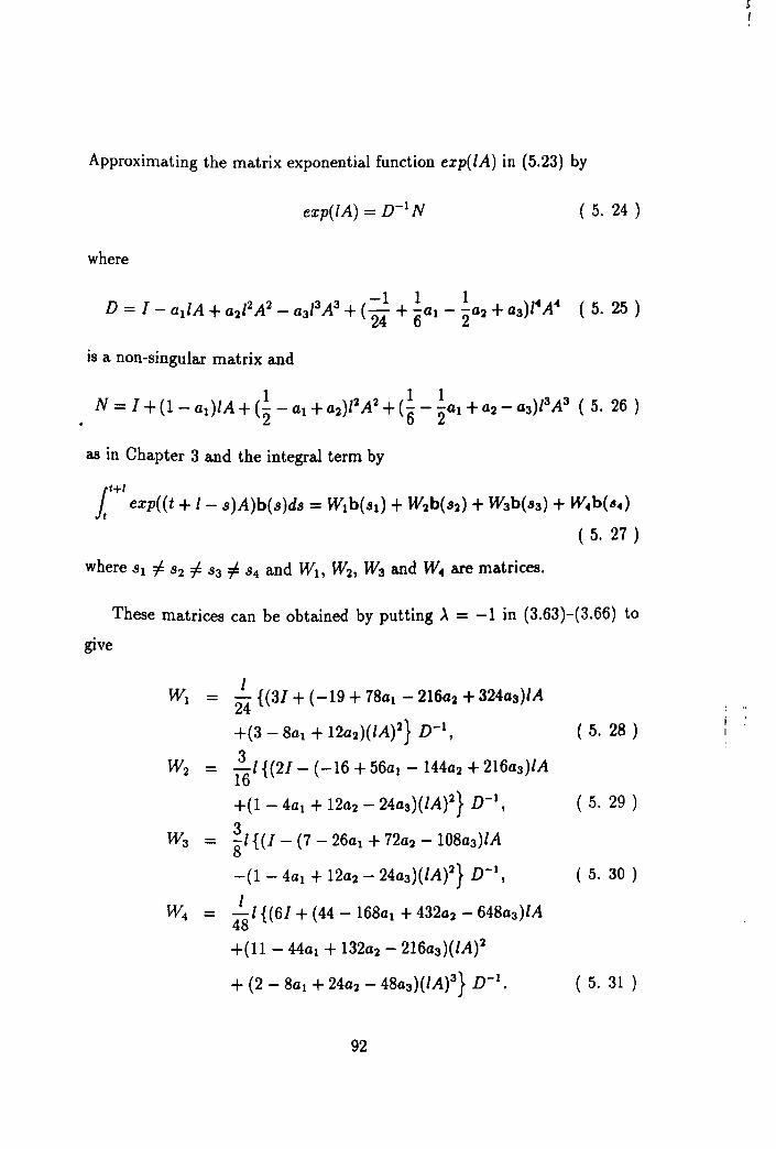
Approximating the matrix exponential function exp(lA) in (5.23) by
exp(lA) = n- I N ( 5. 24 )
where
is a non-singular matrix and
as in Chapter 3 and the integral term by
These matrices can be obtained by putting ,\ = -1 in (3.63)-(3.66) to
give
1 WI = 24 {{31 + (-19 + 78al - 216a2 + 324a3)IA
+(3 - 8al + 12a2)(IA)2} n-1, ( 5. 28 )
3 W2 = 161 {{21 - (-16 + 56al - 144a2 + 216a3)IA
+(1 - 4al + 12a2 - 24a3)(IA)2} n- I, ( 5. 29 )
3 Wa - 81 {(I - (7 - 26al + 72a2 - 108a3)IA
-(1 - 4al + 12a2 - 24a3)(lA)2} n-1, ( 5. 30 )
1 W4 - 481 {(61 + (44 -168al + 432a2 - 648a3)IA
+(11 - 44al + 132a2 - 216a3)(IA)2
+ (2 - 8a1 + 24a2 - 48aa)(lA)3} n-1• ( 5. 31 )
92

Hence (5.23) can be written as
I 2 U(t + /) = exp(lA)U(t) + W1b(t) + W2b(t + 3) + W3b(t + 31) + W.b(t + I).
( 5. 32 )
5.2 Algorithm
The algorithm is similar to that detailed in chapter 3 but it is included for
completeness. Assuming that rt, r2, r3 and r. (ri :F 0) are the real zeros of
( 5. 33 )
then D given by (5.25) can be factorized as
/ I I I D = (I - -A)(I - -A)(J - -A)(I - -A)
rl r2 r3 r. ( 5. 34 )
and then (5.68) can be written in partial-fraction form as
U(t + /) = {Al(I - .i.Atl + A2(I - .i.Atl
rl r2
/ 1 I I} () + A3(J - -At + A.(I - -At U t r3 r.
+ - B1(I - -At + B2(I - -A)-I { I 1 I 1
24 rl r2
+ B3(I - .i.Atl + B.(I - .i.Atl} bet) r3 r.
+ 2./ {CI(J - .i.A)-l + C2(J - .i.At l
16 rl r2
+ C3 (I - .i.Atl + C.(J - .i.Atl} bet + ~) r3 r. 3
+ ~l {Dl (J - .i.Atl + D2 (J - .i.A)-1 8 ~ ~
+ D3(I - .i.A)-l + D.(J - .i.Atl} bet + -32/) r3 r.
93
I ·.f I"
I L

( 5. 35 )
in which for i = 1,2,3,4
Ai 1 + Piri + P2rl + P3r? - 114 (1") j= 1 -~
j:/:i
B, 3 + P4r, + P5rl - 114 . (1 - !i )'
J = 1 'J
j:/: i
Ci 2 - Pari + P7rl
- 114. (1 - !i) , J = 1 'J
j:/: i
Di 1 - PSri - P9r~
- 114 . (1 - !i) , J = 1 'J
j:/: i
E, 6 + PlOr, + pu rl + pur? = 114 (1 - !a.)
j = 1 'J
j:/: i
where
PI - 1 - at,
1 P2 - '2 - al + a2,
1 al Pa - '6 -"2 + a2 - aa,
P4 = -19 + 78al - 216a2 + 324a3,
ps = 3 - 8al + 12a2,
P6 = -16 + 56al - 144a2 + 216a3,
P7 - 1 - 4al + 12a2 - 24a3,
ps - 7 - 26al + 72a2 - 108aa,
94

Hence
which gives
where
PlO = 44 - 168al + 432a2 - 648a31
Pu = 11 - 44al + 132a2 - 216a31
U(t + I) - (I - ~/AtlZl + (I - 2.1AtlZ2 rl ri
+ (I - ~/AtlZ3 + (I - ~/AtlZ4' r3 r.
I 3 I Zi = AiU(t) + 24 (Bib(t) + 161Cib(t + '3)
+ ~/Dib(t + ~l) + 4~ Eib(t + I)) i = 1,2,3,4.
95
( 5. 37 )

Let
then
and
1 1 (I - -IAt Zi = Yi, i = 1,2,3,4 ri
1 (I - -IA)Yi = Zi, i = 1,2,3,4
ri
in which Yl, Y2, Y3 and Y4 are the solutions of the systems
(/ - .!.-\IA)Yi = Zi, i = 1,2,3,4 ri
( 5. 38 )
( 5. 39 )
( 5. 40 )
respectively. This algorithm is presented in tabular form in Table 5.1.
5.3 Numerical Example
In this section a representative of many other methods based on (5.24) will
only be used. Taking
and 547
a3 = 600
it is found that
rl = 2.1883713223893, r2 = 2.3398749224808
r3 = 2.18837132239, r4 = 2.33987492248
are the real zeros of (5.69). These values produce
Al = -176.18490160503, A2 = 2051.1048759736,
96
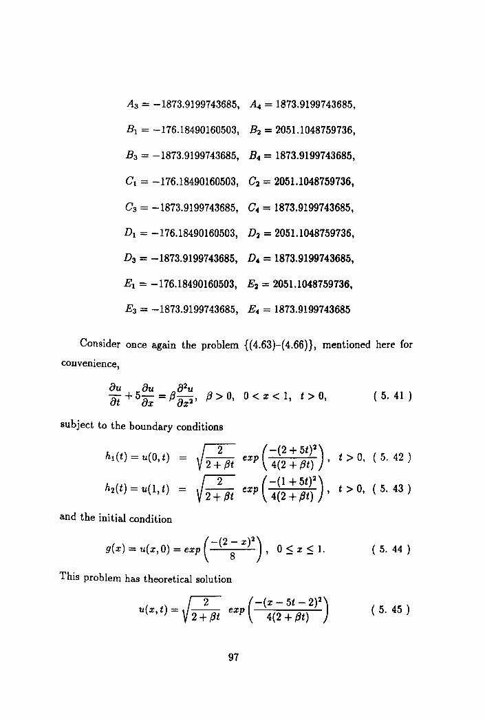
A3 = -1873.9199743685, A .. = 1873.9199743685,
Bl = -176.18490160503, B2 = 2051.1048759736,
B3 = -1873.9199743685, B .. = 1873.9199743685,
C1 = -176.18490160503, C2 = 2051.1048759736,
C3 = -1873.9199743685, C .. = 1873.9199743685,
Dl = -176.18490160503, D2 = 2051.1048759736,
D3 = -1873.9199743685, D. = 1873.9199743685,
El = -176.18490160503, E2 = 2051.1048759736,
E3 = -1873.9199743685, E .. = 1873.9199743685
Consider once again the problem {(4.63)-(4.66)}, mentioned here for
convenience,
( 5. 41 )
subject to the boundary conditions
h1(t) = u(O, t) = J2 (-(2+5t)2) V 2"+ji exp 4(2 + ,Bt) , t > 0, (5. 42 )
~ (-(1 + 5t)2) - V 2"'+"Pt exp 4(2 + pt) , t > 0, (5. 43 )
and the initial condition
g(x) = u(x,O) = exp (-(2; X)2) , 0 $ x :5 1. ( 5. 44 )
This problem has theoretical solution
J2 (-(X - 5t - 2)2) u(x, t) = V 2"+ji exp 4(2 + ,Bt) ( 5. 45 )
97

(see Jain et el. [19]). Using the Algorithm developed in Section 5.2 with
the information given at the beginning of this section the problem {(5.41)
(5.45)} is solved for h = 0.1,0.05,0.025,0.01,0.005 and 1=0.1,0.05,0.025,
0.01,0.005 using f3 = 1000. In these experiments the method behaves smoothly
with third-order accuracy over the whole interval 0 ~ x ~ 1 and no contrived
oscillations are observed. Maximum errors at time t=0.5 are observed at the
mid-point of the region except for very small values of h and I and are given
in Table 5.2. For h = 0.05 and I = 0.001 the maximum error and relative
percentage error obtained are -0.980D-14 and -0.157D-1O respectively at
point 8 of the discretization. It is noticed that the numerical solution crosses
the analytical solution in this experiment but no oscillations are observed.
The numerical solutions for h = 0.1 and 1= 0.1 at time t = 0.5 is depicted
in Figure 5.1.
98
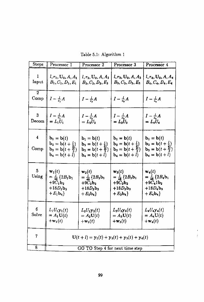
Table 5.1: Algorithm 1
Steps Processor 1 Processor 2 Processor 3 Processor 4
1 I,rl, Uo,A,Al I, r2, Uo, A, A2 I, r3, Uo, A, A3 I, r .. , Uo, A, A .. Input B l , Cl , D l , El B2, C2, D2, E2 B3 , C3 , D3, E3 B ... C .. , D .. , E ..
2 Comp I - .LA
rl I - .LA
r2 I -.LA
ra I - .LA
r,
3 I - .LA I - .LA I -LA I - .LA Decom
rl r2 ra r, = LlUl = L2U2 = L3U3 = L .. U ..
4 b I = b(t) bl = b(t) b l = b(t) b l = b(t) b2 = b(t + 1) b2 = b(t + i) b2 = b(t + 1) b2 = b(t + 1)
Comp b3 = b(t +~) b3 = b(t +-/) b3 = b(t +~) b3 = b(t + ~) b4 = b(t + I) b4 = b(t + 1) b4 = b(t + I) b .. = b(t + I)
5 wt{t) W2(t) W3(t) w .. (t) Using = f8 {2Bl b l = is {2B2bl = is {2B3b l = .. 's {2B .. b1
+9Cl b2 +9C2b2 +9C3b2 +9C .. lb2
+18D1b3 +18D2h3 +18D3h3 +18D .. h3
+El b4 } +E2b .. } +E3b4 } +E.b .. }
6 LIUlYl(t) L2U2Y2(t) L3U3Y3(t) L4U4Y4(t) Solve = Al U(t) = A2U(t) = A3U(t) = A .. U(t)
+Wl (t) +W2(t) +W3(t) +W4(t)
7 U(t + I) = Yl(t) + Y2(t) + Y3(t) + Y4(t)
8 GO TO Step 4 for next time step
99

Table 5.2: Maximum errors for Example 1 at t = 0.5
h 0.1 0.05 0.025 0.01 0.005 N 9 19 39 99 199
1=0.1 -0.107D-7 -0.107D-7 -0.107D-7 -0.107D-7 -0.107D-7 5 10 20 50 100
1=0.05 -0.10SD-S -0.10SD-S -0.107D-8 -0.108D-S -0.107D-S 5 10 20 50 100
1=0.025 -0.119D-9 -0.119D-9 -0.1l9D-9 -0.117D-9 -0.115D-9 5 10 20 50 100
1=0.01 -0.650D-ll -0.645D-11 -0.646D-l1 -0.555D-l1 -0.602D-ll 5 10 20 51 107
1 = 0.005 -0.660D-12 -0.61SD-12 -0.669D-12 -0.S15D-12 -0.709D-13 5 10 20 49 80
100

Figure 5.1 0.0628r---,----,---,------r--r---'T"'"----r--...,..----.----,
0.0627
0.0626
::l 0.0626
0.0626
0.0624~-......I---.l----L.-_...l..----1..-_...L..-_---L-_..J.----L----' o 1 2 3 456 Space Steps
7 8 9
Figure 5.1: Numerical solution of example 1 for h = 0.1, and 1= 0.1 a.t timt" t=0.5
101
10

Chapter 6
Third-Order Finite-Difference Methods for Second-Order Hyperbolic Partial Differential Equations
6.1 The Model Problem
Consider the one-dimensional initial/boundary-value (I BV P) problem con
sisting of the partial differential equation (P DE)
{Pu f)2u 2
ot2 = C ox2' 0< x < X, t > ° (6. 1 )
in which u = u(x, t) subject to the homogeneous boundary conditions
u(O,t) = u(X,t) = 0, t > 0
and the initial conditions
u(x,O) 8u(x, 0)
8t
= g(x),
= f(x),
102
( 6. 2 )
( 6. 3 )
( 6. 4 )
j
in which g(x) and f(x) are given continuous functions of x.
There will exist discontinuities between the initial and the boundary
conditions if
g(O) ::I 0 and/or g(X)::I 0.
6.2 Discretization of R U oR
The region R (the open rectangle bounded by the lines x = 0, t = 0, x = X)
and its boundary 8R are covered by a grid, consisting of lines parallel to the
time axis and lines parallel to the space axis (x-axis). Assuming h > 0 and
I > 0, the interval 0 ~ x ~ X is divided into N + 1 subintervals each of width
h, so that
(N + l)h = X
and the time t ;::: 0 is divided into equal time steps of length I. The parameter
h is called the space-step and I is the time-step. Each discrete mesh point
has co-ordinates of the form
for m =: 0,1,2, ... , N + 1 and n = 0,1,2, ....
6.3 The Method
Replacing the space derivative 82;~!t) in the P DE (6.1) by the third-order
difference approximations [38]
82u{x, t) 1 8x2 = 12h2 {ll u(x - h, t) - 20 u(x, t) + 6 u{x + h, t)
103

h3 85u(x, t) + 4u(x + 2h, t) - u(x + 3h, tn + 12 8x5
+ O(h4)as h~O ( 6. 5 )
for the mesh points (xm, tn) with m = 1,2, ... ,N - 2,
1 = I2h2 {u(x - 3h,t) - 6u(x - 2h,t) + 26u(x - h,t)
h3 85u(x t) - 40 u(x, t) + 21 u(x + h, t) - 2u(x + 2h, tn + 12 8x'"
+ O(h4) as h ~ 0 ( 6. 6 )
for the mesh point (XN-t. tn) and
1 - I2h2 {2 u(x - 4h, t) - 11 u(x - 3h, t) + 24 u(x - 2h, t)
h3 8'u(x, t) - I4u(x - h,t) -IOu(x,t) - 9u(x + h,t)} + 12 8x"
+ 0 ( h 4 ) as h ~ 0 ( 6. 7 )
for the mesh point (XN, tn), provides a system of N second-order ordinary
differential equations (ODE's) which can be written in matrix-vector form
as
with initial conditions
and
in which
tPU(t) = AU(t) t > 0 dt2 '
U(O) = g
dU(O) = f(x) dt
U(t) - [Ut (t), U2(t), ... , UN(t)]T, g - [g(Xt},g(X2), ... ,g(XN)]T, f = [J(Xt},/(X2), ... ,/(XN)]T,
104
( 6. 8 )
( 6. 9 )
( 6. 10 )
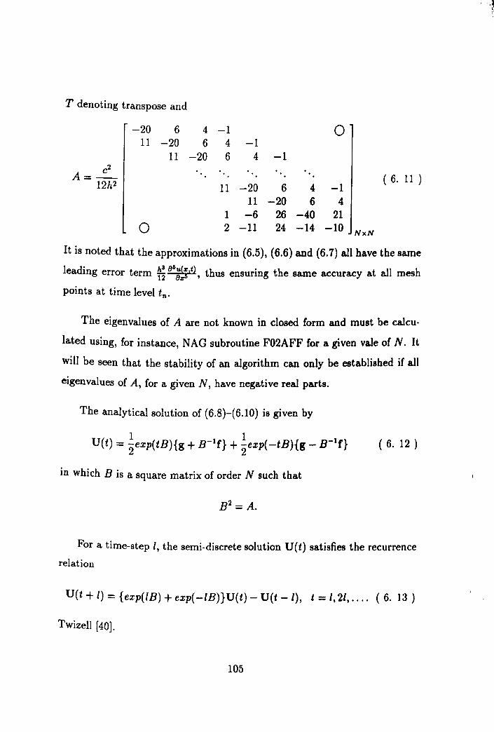
T denoting transpose and
-20 6 4 -1 0 11 -20 6 4 -1
11 -20 6 4 -1 c2
A=- ( 6. 11 ) 12h2 11 -20 6 4 -1 11 -20 6 4
1 -6 26 -40 21 0 2 -11 24 -14 -10
NxN
It is noted that the approximations in (6.5), (6.6) and (6.7) all have the same
leading error term ~~ 86;~,t), thus ensuring the same accuracy at all mesh
points at time level tn.
The eigenvalues of A are not known in closed form and must be calcu
lated using, for instance, NAG subroutine F02AFF for a given vale of N. It
will be seen that the stability of an algorithm can only be established if all
eigenvalues of A, for a given N, have negative real parts.
The analytical solution of (6.8)-(6.10) is given by
11_ U(t) = "2exp(tB){g + B-1f} + "2exp( -tB){g - B If}
in which B is a square matrix of order N such that
( 6. 12 )
For a time-step I, the semi-discrete solution U(t) satisfies the recurrence
relation
U(t + I) = {exp(lB) + exp( -IB)}U(t) - U(t - I), t = 1,2/, .... (6. 13 )
Twizell [40].
105
· .; ~.

6.4 Solution at the First Time-Step
Using Taylor's series
Substituting t = I in (6.12) gives
1 1 U(l) = 2exp(lB){g + B- l f} + 2exp( -IB){g - B- l f} ( 6. 14 )
which can be written as
1 1 U(l) = 2 {exp(lB) + exp( -IB)} g + 2 {exp(lB) - exp( -IB)} B-1f.
( 6. 15 )
Now
and
exp( -IB) = I -IB+.!.12 B2_.!./3 B3+~/4B4_~/5B5+~z6B6_ ~f B7 + ... 2! 3! 4! 5! 6! 7!
( 6. 17 )
Thus
( 6. 18 )
and
exp(lB) - exp( -IB) = 2 (IB + ~/3 B3 + ~/5 B 5 + ~z7 B7 + ) (6. 19 ) 3! 5! 7! " .
or
{Ill} exp(lB) - exp( -IB) = 2 1+ 3! /2 B2 + 5! I"B4 + 7! f3 B6 + . .. lB.
( 6. 20 )
106

Substituting these values in (6.15) gives
U(l) (1221[44 1 166 ) - 1+ ,[ B +, B + 6,rB + ... g 2. 4. .
( 1 2 2 1 4 4 1 r6B6 ) If + 1+ ,/ B + ,I B + 7"- + ... 3. 5. .
( 6. 21 )
or
6.5 Rational Approximation to Matrix Exponential Function
To approximate the matrix exponential function in (6.13) consider the ratio
nal approximant (1.1)
E3( fJ) = 1 + (1 - adO + (il
- al + a2)02 . ( 6. 23 ) 1 - atO + a202 - (-6 - T + a2)03
where al and a2 are parameters. Let
( 6. 24 )
and
1- atO + a202 - (~- ~l + a2)()3 = q(O). ( 6. 25 )
Now consider the sum
_ p(fJ) + p( -0) = P(O) q( 0) q( -0) Q( 0)
( 6. 26 )
where
( 6. 27 )
107
i I

and
Q( 0) q( 0) x q( -0)
- 1 + (2a2 - an02 - (~al - a~ + 2ala2 - an04
1 1)2 6 (6 + a2 - 2"a1 O. ( 6. 28 )
Assuming 4> = 02 gives
( 6. 29 )
and
( 6. 30 )
6.6 Accuracy
It is convenient to consider the single initial-value problem
D2y == y"{t) = f(t,y),t > to, y{tO) = Yo, y'(tO) = zo ( 6. 31 )
where y = y(t) and D2 = ~. The numerical solution to this problem may
be obtained from the formula
y(t + I) = {exp(lD) + exp(-ID)}y{t) - y(t -I). ( 6. 32 )
Replacing 0 by ID in (6.26) and then substituting the value of exp(lD) + exp( -ID) in (6.32) leads to
Yn+l =
108

( 6. 33 )
in which Yn is an approximation to y(tn). The associated local truncation
error is
L[y(t); I)
( 6. 34 )
which may be expanded as a Taylor series about t to give
L[ () ] I 1 II 1 3 III 1 " 1111 1 5 11/11
Y t ; 1 = y(t) + Iy (t) + 2r~y (t) + '6 1 y (t) + 241 y (t) + 1201 Y (t)
1 6 111111
+720 1 y + ... ( 2 )[2{ "() 1 III() 1 (~ IIII() 1/3 1I111( ) 1 1" 111111 - a 1 - 2a2 y t + y t + 2 y t + 6 y t + 24 Y
+ ... }
109

1 [6 111111 +720 y - ...
+ (2 2) 2{ "() 1 III() 1/2 IIII() 1/3 1II11( ) 1 I" 111111 a2 - a1 1 y t - Y t + 2 y t - '6 y t + 24 Y
- ... }
After simplification (6.35) becomes
1 1 4 1111 6 L[y(t); 1] = (-4 + 2a1 - a2)1 Y (t) + 0(1 ). ( 6. 36 )
6.7 Development of Parallel Algorithm
Suppose that ri(i = 1,2,3,rj =f:. 0) are distinct real zeros of Q(tI» defined by
(6.30) then
3 ( 1)-1 exp(lB) + exp( -IB) = ~ c; 1 - rj A ( 6. 37 )
where B2 = A and Cj (i = 1,2,3), the partial-fraction coefficients, are defined
by
( 6. 38 )
in which
P(rd - 2{1+(2a2-a~+~)rj 3 2 2 1 2 1 2} + (2a2 - 2a1a2 + a2 - 3a1 + 2 a1 + '6 )rj
i = 1,2,3. So, using (6.31) in (6.13) gives
(
3 ( 12) -1) U(t + I) = ~ c; 1 - Tj A U(t) - U(t -I). ( 6. 39 )
110

t = 1,21,31,. '" Now let
( 12)-1
Ci 1 - r. A U(t) = Wi(t), i = 1,2,3, ( 6. 40 )
Then the systems of linear equations
(1 - ~: A) Wi(t) = csU(t), i = 1,2,3 ( 6. 41 )
can be solved for wi(t)(i = 1,2,3) on three different processors simultane
ously, and finally
3
U(t + 1) = Ew.(t) - U(t -1) t = 1,21,31, .... ( 6. 42 ) .=1
This algorithm is given in tabular form in Table 6.1.
6.8 Numerical Examples
In this section a representative of many other methods based on (6.23) will
only be used. So taking at = :~ and a2 = i~ as before gives
rl = 4.788969044658795, r2 = 5.475014652818082, r3 = 5.554994179738606
as the real zeros of (6.30). Using these values in (6.38) gives
Cl = -352.369803216, C2 = 4102.20974857, C3 = -3747.83994535
6.8.1 Example 1
Considering the one dimensional wave equation with constant coefficients
(6.1) and taking X = 1, g(x) = lsin(1rx) and f(x) = 0 in {(6.1)-(6.4)} the
model problem becomes
( 6. 43 )
111
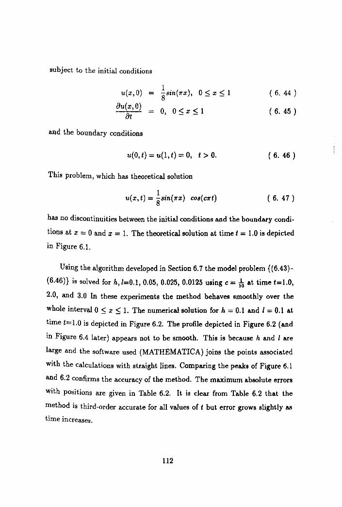
subject to the initial conditions
u(x,O)
au(x, O) at
and the boundary conditions
- ~Sin(1rx), 0 ~ x ~ 1
- 0, 0 ~ x ~ 1
u(O,t) = u(l,t) = 0, t > O.
This problem, which has theoretical solution
u(x, t) = ~Sin(1rx) cos (C1I"t)
( 6. 44 )
( 6. 45 )
( 6. 46 )
( 6. 47 )
has no discontinuities between the initial conditions and the boundary condi
tions at x = 0 and x = 1. The theoretical solution at time t = 1.0 is depicted
in Figure 6.1.
Using the algorithm developed in Section 6.7 the model problem {(6,43)
(6.46)} is solved for h, 1=0.1,0.05, 0.025, 0.0125 using c = }10 at time t=1.0,
2.0, and 3.0 In these experiments the method behaves smoothly over the
whole interval 0 :$ x :$ 1. The numerical solution for h = 0.1 and I = 0.1 at
time t=1.0 is depicted in Figure 6.2. The profile depicted in Figure 6.2 (and
in Figure 6.4 later) appears not to be smooth. This is because h and I are
large and the software used (MATHEMATICA) joins the points associated
with the calculations with straight lines. Comparing the peaks of Figure 6.1
and 6.2 confirms the accuracy of the method. The maximum absolute errors
with positions are given in Table 6.2. It is clear from Table 6.2 that the
method is third-order accurate for all values of t but error grows slightly as
time increases.
112
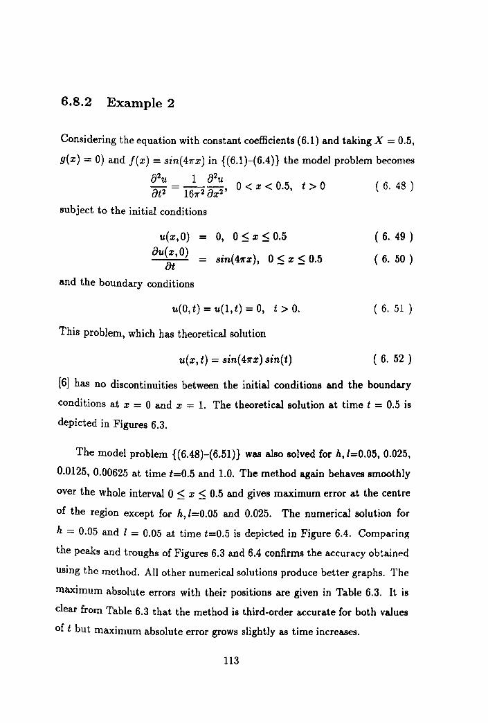
6.8.2 Example 2
Considering the equation with constant coefficients (6.1) and taking X = 0.5,
g(x) = 0) and f(x) = sin(411"x) in {(6.1)-(6.4)} the model problem becomes
{)2u 1 82u 8t2 = 1611"2 8x2 ' 0 < x < 0.5, t > 0
subject to the initial conditions
0, 0 ~ x ~ 0.5 u(x, 0) -8u(x, 0)
- sin(42rx), 0 ~ x ~ 0.5 at
and the boundary conditions
'11(0, t) = '11(1, t) = 0, t > O.
This problem, which has theoretical solution
u(x, t) = sin{41rx) sin(t)
( 6. 48 )
( 6. 49 )
( 6. 50 )
( 6. 51 )
( 6. 52 )
[6] has no discontinuities between the initial conditions and the boundary
conditions at x = 0 and x = 1. The theoretical solution at time t = 0.5 is
depicted in Figures 6.3.
The model problem ({6.48)-(6.51)} was also solved for h,I=0.05, 0.025,
0.0125, 0.00625 at time t=0.5 and 1.0. The method again behaves smoothly
over the whole interval 0 ~ x ~ 0.5 and gives maximum error at the centre
of the region except for h,I=0.05 and 0.025. The numerical solution for
h = 0.05 and I = 0.05 at time t=0.5 is depicted in Figure 6.4. Comparing
the peaks and troughs of Figures 6.3 and 6.4 confirms the accuracy obtained
using the method. All other numerical solutions produce better graphs. The
maximum absolute errors with their positions are given in Table 6.3. It is
clear from Table 6.3 that the method is third-order accurate for both values
of t but maximum absolute error grows slightly as time increases.
113

f 1
Table 6.1: Algorithm 1
Steps II Processor 1 I Processor 2 I Processor 3
1 I, rh C., I, r2, C2, I, ra, C3, Input Uo,A Uo,A Uo,A
2 Compute 1- .l..A
rl 1- .l..A
r2 1- .l..A
r3
3 1- .l..A 1- .l..A I - .l..A Decompose
rl r2 r3
= LtUt = L2U2 = L3U3
4 Find Solution at the first time step
5 LtUtWt(t) L2U2W2(t) L3U3W3(t) Solve = Cl U(t) = C2 U(t) = C3U(t)
6 U(t + 1) = Wl(t) + W2(t) + W3(t) - U(t -I)
7 GO TO Step 5 for next time step
114

Table 6.2: Maximum absolute errors for Example 1
II 9 19 39 79
0.1 0.05 0.025 0.0125
t=1.0 0.124847D-4 O.177997D-5 0.231373D-6 O.305657D-7 Positions 1 17 4 72
I: I
t=2.0 0.399566D-4 O.612910D-5 0.785875D-6 O.106804D-6 Positions 8 16 7 66
t=3.0 0.741103D-4 O.107269D-4 0.135521D-5 0.190258D-6 Positions 7 15 9 61
POlilion. are Ihowll by Ipace .Iepl.
Table 6.3: Maximum absolute errors for Example 2
N 9 19 39 79 h,l 0.05 0.025 0.0125 0.00625
t = 0.5 0.386306D-3 O.512678D-4 0.650840D-5 0.818575D-6 Positions 4 9 20 40
t = 1.0 0.286251D-2 O.379984D-3 0.482384D-4 0.606705D-5 Positions 4 9 20 40
POlilioll1 are Ihowll by Ipace .Iepl.
115

Figure 6.1 0.12r---r----.----.---.-~~~--r---.---~----,---,
0.1
0.08
:J 0.06
0.04
0.02
0.2 0.3 0.4 0.5 x
0.6 0.7 0.8
Figure 6.1: Theoretical solution of example 1 for time t=l.O
116
0.9 1

Figure 6.2 O.14r----r----r---~----~--~----~--_,----._--_.,_--~
0.1
1 2 3 4 5 6 7 8 9 10 Space Steps
Figure 6.2: Numerical solution of example 1 for h = 0.1, and 1= 0.1 at time t=1.0
117
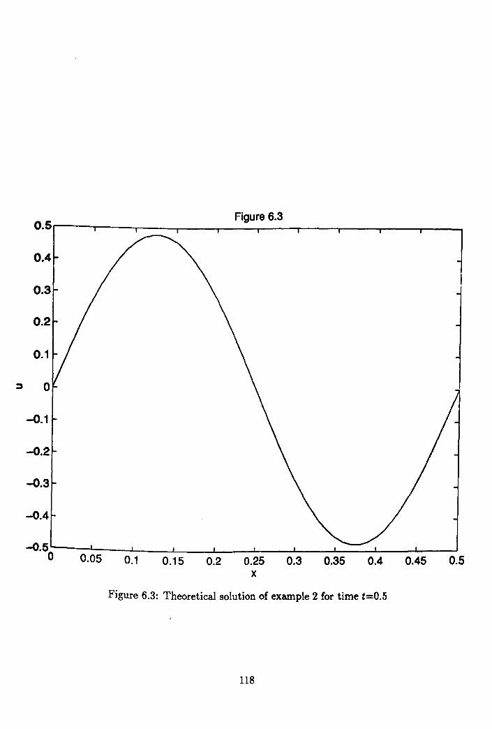
Figure 6.3 0.5r----.----r---~----~--~--_.----,_--~----~--~
0.4
0.3
0.1
::J
-0.1
-0.2
-0.3
-0.4
-0.5 0 0.05 0.1 0.15 0.2 0.25 0.3 0.35 0.4 0.45 0.5
x
Figure 6.3: Theoretical solution of example 2 for time t=O.5
118

Figure 6.4 0.5r----r----r---~----~--~--_,----,_--_,----~--_,
0.1
-0.1
-0.2
-O.5~--~--~~--~--~----J---~----~--~----~--~ o 1 2 3 456 Space Steps
7 8 9
Figure 6.4: Numerical solution of example 2 for h, 1=0.05 at time t=0.5
119
10

Chapter 7
Fourth-Order Finite-Difference Methods for Second-Order Hyperbolic Partial Differential Equations
7.1 The method
Considering the model problem of Chapter 6 consisting of the partial differ-
ential equation
821.1. 282
1.1. 8t2 = C 8x2 ' 0 < x < X, t > 0 (7. 1 )
in which 1.1. = u(x, t) subject to the boundary conditions
u(O, t) = u(X, t) = 0, t > 0
and the initial conditions
u(x,O) 8u(x, 0)
8t
= g(x),
- lex),
120
0:5 x:5 X,
( 7. 2 )
( 7. 3 )
( 7. 4 )

in which g(x) and f(x) are given continuous functions of x, the method
can be developed by replacing the space derivative 83;£2,t) in (7.1) by the
fourth-order difference approximations [39)
(j2u(x, t) 8x2
1 '" 12h2 {9u(x - h, t) - 9u(x, t) - 19u(x + h, t)
+ 34u(x + 2h, t) - 21u(x + 3h, t) + 7u(x + 4h, t) h4 lJ6u(x, t)
- u(x + 5h, tn + 90 8x6
( 7. 5 )
for the mesh point (XI, tn),
82u(x, t) 1 {)x2 '" 12h2 {-u(x - 2h, t) + 16u(x - h, t) - 30u(x, t)
h4 lJ6u(x, t) + 16u(x + h, t) - u(x + 2h, tn + 90 8x6
( 7. 6 )
for the mesh points (xm' tn) with m = 2,3, ... , N - 1 and
()2u(x, t) 1 {)X2 '" 12h2 {-u(x - 5h, t) + 7u(x - 4h, t) - 21 u(x - 3h, t)
+ 34u(x - 2h, t) - 19u(x - h, t) - 9u(x, t) + 9u(x + h, t)}
+ ~~ ()6~~~,t) + O(h5)as h ~ 0 ( 7. 7 )
for the mesh point (XN, tn), provides a system of N second-order ordinary
differential equations which can be written in vector-matrix form as
with initial conditions
and
in which
cPU(t) = AU(t) t > 0 dt2 '
U(O) = g
dU(O) = f(x) dt
121
( 7. 8 )
( 7. 9 )
( 7. 10 )
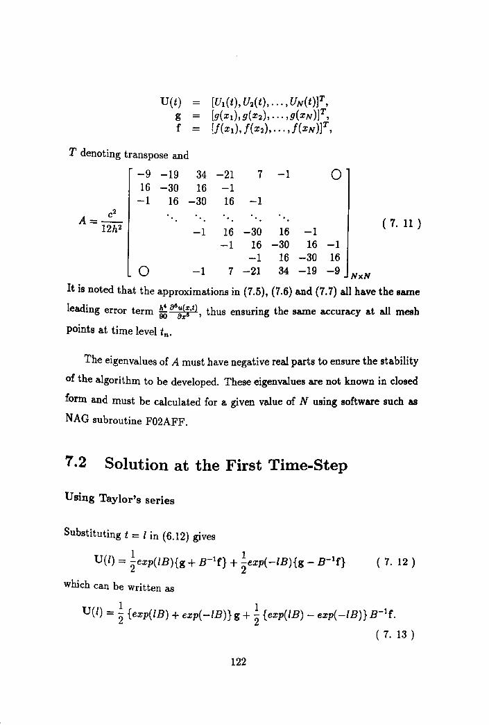
U(t) - [U1(t), U2(t), ... , UN(t)]T, g - [g(Xl),g(X2),'" ,g(XN)]T, f [J(Xl), !(X2),'" ,!(XN)]T,
T denoting transpose and
-9 -19 34 -21 7 -1 0 16 -30 16 -1 -1 16 -30 16 -1
-1 16 -30 16 -1 ( 7. 11 )
-1 16 -30 16-1 -1 16 -30 16
o -1 7 -21 34 -19 -9 NxN
It is noted that the approximations in (7.5), (7.6) and (7.7) all have the same
leading error term ~ 88;~:.t), thus ensuring the same accuracy at all mesh
points at time level tn.
The eigenvalues of A must have negative real parts to ensure the stability
of the algorithm to be developed. These eigenvalues are not known in closed
form and must be calculated for a given value of N using software such as
NAG subroutine F02AFF.
7.2 Solution at the First Time-Step
U sing Taylor's series
Substituting t = I in (6.12) gives
1 1 U{l) = 2exp{lB){g + B- l f} + 2exp( -IB){g - B- l f} ( 7. 12 )
which can be written as
1 1 U{l) = 2 {exp(lB) + exp( -IB)} g + 2 {exp{lB) - exp( -IB)} B-1r.
( 7. 13 )
122

Now
and
Thus
exp(lB) + exp( -IB) = 2 (I + ~/2 B2 + ~/4B" + i~ B6 + ... ) (7. 16 ) 2. 4. 6.
and
exp(1B) - exp( -IB) = 2 (IB + ~13 B3 + ~/5 B5 + ~f B7 + ... ) (7. 17 ) 3. 5. 7.
or
exp{lB)-exp( -IB) = 2 {I + i/2 B2 + ~/4B4 + 7\ZSB6 + ... } IB ( 7. 18 ) 3. 5. .
Substituting these values in (7.13) gives
or
U(l)
U(l) - (I + ;,12A + :,/4A2 + 0(16») g
+ (I + ;,12A + 0(15») If.
123
( 7. 19 )
( 7. 20 )

7.3 Rational Approximation to Matrix Exponentional Function
To approximate the matrix exponential functions in (7.13) consider the ra
tional approximant (1.2), given for a real scalar (), by
E (() = 1 + (1 - ad() + (! - at + a2)()2 + a -!al + a2 - a3)()3 (7. 21 ) 4 ( 1 G G )04 • 1 - al() + a2()2 - a3()3 + -2,i + It - !f + a3
where at a2 and a3 are parameters . Let
and
1 fJ 2 3 1 at a2 )()4 (fJ) - al + a2() - a3() + (-- + - - - + a3 = q . 24 6 2
( 7. 23 )
Now consider the sum
p( 0) + p( -() = P( () - q( 0) q( -0) Q( 0)
( 7. 24 )
where
and
Q( () - q( () x q( -()
( 7. 26 )
124
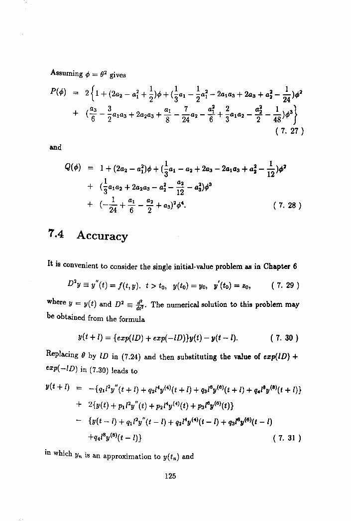
and
Q(¢»
( 7. 28 )
7.4 Accuracy
It is convenient to consider the single initial-value problem as in Chapter 6
D2 " '( ) y = Y (t) = f(t, y). t > to, y(to) = Yo, Y to = %0, ( 7. 29 )
where y = yet) and D2 = ,. The numerical solution to this problem may
be obtained from the formula
yet + I) = {exp(lD) + exp(-ID)}y(t) - yet -I). ( 7. 30 )
Replacing () by ID in (7.24) and then substituting the value of exp(lD) + exp( -ID) in (7.30) leads to
yet + I) - -{ql /2y"(t + I) + q2/4y(4)(t + 1) + Q3 /6y(6)(t + I) + q,,/8y(8)(t + I)}
+ 2{y(t) + Pl /2y"(t) + p2/4y(4)(t) + P316y(6)(t)}
- {yet - I) + Ql /2y"(t -I) + Q2/4y(")(t -I) + Q3z6y(6)(t -I)
( 7. 31 )
in which Yn is an approximation to y( t n ) and
125

PI = P2 = ]13=
ql = q2 = q3 = q4 =
The associated local truncation error is
or
L[y(t); /] = yet + I) + q1/2y"(t + I) + q21"y(4)(t + I) + q3tJy(8)(t + I)
+q4/8y(8)(t + I)
- 2{y(t) + pt/2y" (t) + P2/4y(4)(t) + P3fy(8)(t)}
+ {yet -I) + qt/2y"(t -I) + q2/4y(4)(t - I) + q3tJy(8)(t -I)
+q4/Sy(8)( t - In ( 7. 32 )
L[y(t); I] - yet + I) + yet -I)
+ qt/2{y"(t + I) + y"(t -I)}
+ Q2 /4 {y(4)(t + I) + y(4)(t - In
+ Q3tJ {y(6)( t + I) + y(6)( t - I)}
+ Q4 /8 {y(S)(t + I) + y(8)(t - I)}
- 2{y(t) + Pt/2y"(t) + P2/4 y(4)(t) + P3tJy(6)(t)} ( 7. 33 )
which may be expanded as a Taylor series about yet) to give
L[y( t); I]
126
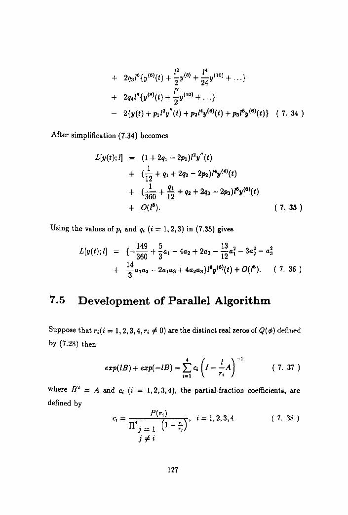
[2 14 + 2q316{y(6)(t) + "2 y(8) + 24 y(lO) + ... }
12 + 2q4[8{y(8)(t) + "2y (lO) + ... }
- 2{y(t) + Pl/2y"(t) + P2/4y(4)(t) + P3f1y(6)(t)} (7. 34 )
After simplification (7.34) becomes
L[y(t); I] - (1 + 2ql - 2Ft )[2y" (t) 1
+ (12 + ql + 2q2 - 2P2)l"y{")(t)
+ (_1_ + !!! + q2 + 2q3 - 2P3)fly{6)(t) 360 12
+ 0(/8). ( 7. 35 )
Using the values of Pi and q, (i = 1,2,3) in (7.35) gives
L[y( t)j I] 149 5 13 2 2 2
- {- 360 + 3'al - 4a2 + 2a3 - 12 a l - 3a2 - a J
+ 134
ala2 - 2ala3 + 4a2a3}fly(6)(t) + 0(18). ( 7. 36 )
7.S Development of Parallel Algorithm
Suppose that r,( i = 1,2,3,4, r, :f: 0) are the distinct real zeros of Q( <p) defined
by (7.28) then
" ( I)-I exp(lB) + exp( -IB) = ~ Ci J - ri A ( 7. 37 )
where B2 = A and Ci (i = 1,2,3,4), the partial-fraction coefficients, arc
defined by
P(rd . Ci = ()' ,= 1,2,3,4 rr" . 1 - !L
J = 1 r J
( 7. 3S )
j =F i
127

in which
i = 1,2,3,4. So, using (7.37) in (6.13) gives
(
4 ( 12) -1) U(t + I) = ~ ct 1- rj A U(t) - U(t -I), ( 7. 40 )
t = 1,2/,3/, . ... Now let
( 12)-1 Cj 1- rj A U(t) = Wi(t), i = 1,2,3,4 ( 7. 41 )
Then the systems of linear equations
(I - ~:A) Wj(t) = £;U(t), i = 1,2,3,4 ( 7. 42 )
can be solved for wi(t)(i = 1,2,3,4) on four different processors simultane
ously, and finally
4
U(t + I) = LWi(t) - U(t -I) t = 1,2/,3/, .... ( 7. 43 ) i=l
This algorithm is given in tabular form in Table 7.1.
7.6 Numerical Examples
As in Chapter 6, a representative of methods based on (7.21) will be USN!.
SO, taking c = 0.1, al = ~, a2 = ~ and a3 = ~ as before gives
rl = 0.879057959205939, r:z = 3.293208163041111,
r3 = 4.000000000000405, r. = 5.109949525352754
128

as the real zeros of (7.28). Using these values in (7.38) gives
Cl = -0.243656912725722D + 03, C2 = 0.506244897959209D + 03,
C3 = -0.262087555440892D + 03, c.c = 0.149957020740562D + 01
7.6.1 Example 1
Considering the one dimensional problem {(7.1)-(7.4)} with X = 1, g(x) = ~sin(1I'x) and f(x) = ° the model problem becomes
82u 82u - c2
8t2 - 8x2 '
subject to the initial conditions
0< x < 1, t > 0
u(x,O) = ~sin(1I'x), 0:5 x:5 1,
8u(x,0) 8t = 0, 0:5x:51,
and the boundary conditions
u(O,t) = u(1,t) = 0, t > O.
This problem has theoretical solution
u(x,t) = ~sin(1I'x)cos(crt).
The theoretical solution at time t = 1.0 is depicted in Figure 6.1.
( 7. 44 )
( 7. 45 )
( 7. 46 )
( 7. 47 )
( 7. 48 )
Using Algorithm 1 the model problem {(7.44)-(7.47)} is solved for I, h = 112 , 2
14' 18' ~, using c = 110 at t= 1.0, 2.0 and 3.0. In these experiments
the method behaves smoothly over the whole interval 0 :5 x :5 1 and gives
maximum error at the centre of the region except (or h = Ill' The numerical
solution for h, I = 112 at time t=1.0 is depicted in Figure 7.1. All othf"r
129

numerical solutions produce similar graphs. Maximum absolute error~ with
positions are given in Table 7.2. It is clear from Table 7.2 that the new
method is better than fourth order for larger values of h and I and it is
fourth-order over all. Table 7.2 shows that with the passage of time the
maximum absolute error grows slightly.
7.6.2 Example 2
Considering the one dimensional hyperbolic problem
82u 1 82u 8t2 = 161r2 8x2 ' 0 < x < 0.5, t > 0
subject to the initial conditions
u(x,O) - 0, 0 ~ x ~ 0.5
8u(x,0) _ sin(41rx), 0 ~ x ~ 0.5 at and the boundary conditions
u(O, t) = u(l, t) = 0, t > O.
The theoretical solution of this problem
u(x,t) = sin(41rx)sin(t)
([6]) at time t = 0.5 is depicted in Figure 6.3.
( 7. 49 )
( 7. 50 )
( 7. 51 )
( 7. 52 )
( 7. 53 )
Using again Algorithm 1 the model problem ({7.49)-(7.52)} is solved for
1, h= 214' 4~' ie, 1!2 at t=0.5 and 1.0. In these experiments the method behaves
smoothly over the whole interval 0 ~ x ~ 0.5. The numerical solution for
h, 1=214 at time t=O.5 is depicted in Figure 7.2. All other numerical ~ollltions
produce better graphs. Maximum absolute errors with positions are given
in Table 7.3. It is clear from Table 7.3 that the method is fourth order but
with the passage of time maximum absolute error grows slightly.
130
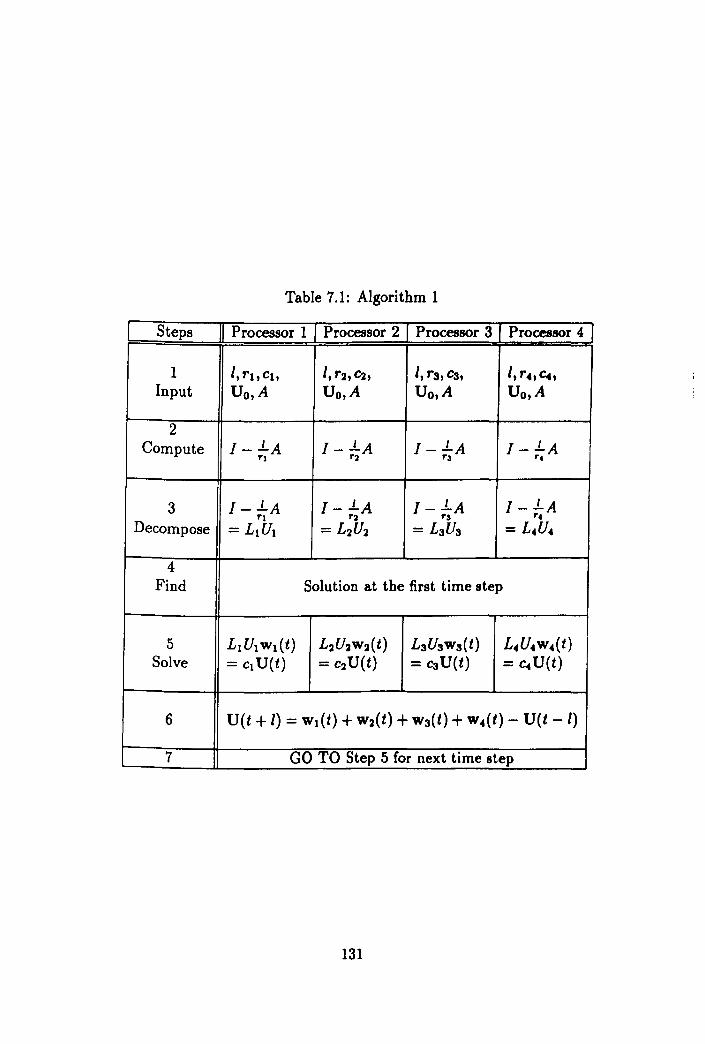
Table 7.1: Algorithm 1
Steps Processor 1 Processor 2 Processor 3 Processor 4
1 I, rl, Cl, l,r2,c2, I, rs, C3, l,r.,4, Input Uo,A Uo,A Uo,A Uo,A
2 Compute I -1.A I -1.A I -1.A I -1.A
rl r2 r3 r,
3 I -1.A I -1.A I -1.A I -.LA rl r2 r3 r,
Decompose = Ll UI = L2U2 = LsUs = L .. U.
4 Find Solution at the first time step
5 L1U1W l(t) L2U2W 2(t) L3U3W 3(t) L.U .. w .. (t) Solve = Cl U(t) = c2U(t) = C3U(t) = c .. U(t)
6 U(t + I) = Wl(t) + W2(t) + ws(t) + w.(t) - U(t -I)
7 GO TO Step 5 for next time step
131

Table 7.2: Maximum absolute errors for Example 1.
I ~,l II 11 23 47 95 J.. 12
.1 24
.1 4A
t=1.0 0.52028D-6 0.19602D-7 0.12301D-8 O.92815D-1O Positions 1,11 12 24 50
t=2.0 O.13930D-5 O.74557D-7 O.46802D-8 0.35069D-9 Positions 1,11 12 24 48
t=3.0 0.24834D-5 O.15392D-6 0.96614D-8 0.72430D-9 Positions 3,9 12 24 48
Po.ilion. a.re .bOWD by .pace "'p"
Table 7.3: Maximum absolute errors for Example 2.
N 11 23 47 95 h,l -i4 1a ~ ski
t = 0.5 0.23782D-4 0.16556D-5 O.65911D-7 OA1566D-8 Positions 1,11 1,23 12,36 72
t = 1.0 0.16556D-3 0.77784D-5 0.488780-6 0.30810D-7 Positions 1,11 6,18 12,36 24,72
132

Figure 7.1 0.12r-------,--------r------~~------._------._------~
0.1
0.08
~0.06
0.04
0.02
O~------~-------L------~------~~------~------~ o 2 4 6 Space Steps
8 10
Figure 7.1: Numerical solution of example 1 for h, 1= 1~ at time t=l.O
133
12

Figure 7.2 0.5r-------~------~------_.------~r_------._------1
0.4
0.3
0.1
::J 0
-0.1
-0.2
-0.3
-0.4
-0.5 0 2 4 6 8 10 12
Space Steps
Figure 7.2: Numerical solution of example 1 for h, I = .} .. at time t=O.5
134
Chapter 8
Summary and Conclusions
8.1 Summary
The main theme of this thesis was to find some new numerical methods which
are stable, require only real arithmetic and are third- or fourth-order accurate
in space and time for parabolic/ hyperbolic partial differential equations and
to develop parallel algorithms for their implementation.
Chapter 1 was written for introductory purposes and covers some general
topics. For example, a basic introduction is given in Section 1.1, an intro
duction to the method of lines, very important in solving time-dependent
partial differential equations, is given in Section 1.2, important notations are
mentioned in Section 1.3, rational approximations to exp(t) are mentioned
in Section 1.4 and some mathematical properties of finite-difference meth
ods, for example, error analysis, consistency, stability and convergence, are
outlined in Section 1.5.
In Chapter 2 a family of third-order numerical methods for the advec
tion equation with constant coefficients was developed. In Section 2.2. thf'
135

model problem is outlined and third-order accuracy in the space component
is achieved at all points of the space discretization in Section 2.3 and a new
governing matrix was obtained. The third-order accuracy in the comple
mentary component is also obtained using a rational approximation to the
matrix exponential function, which can be resolved imto partial fractions,
in Section 2.3. Since efficiency is also an important object of this thesis, a
parallel algorithm which is implementable on an architecture consisting of
three processors is developed in Section 2.4. This chapter is concluded by
numerical examples which show that the methods are very effective. Picto
rial evidence is also appended for support. This method is also modified for
a non-linear problem in Section 2.6 and tested on a numerical example.
In Chapter 3 a family of fourth-order numerical methods for the advection
equation, with constant coefficients, subject to some boundary conditions, is
introduced. Fourth-order accuracy in the space component at all points of the
space discretization is derived in Section 3.1 and a new matrix is obtained.
A rational approximation, involving three parameters, is used to achieve
fourth-order accuracy in the time variable. A parallel algorithm which is
implementable on an architecture consisting of four processors is developed
in Section 3.2. At the end of this chapter the same numerical example!'!,
which are given in Chapter 2, are considered and it is found that numerica.l
results are very accurate. Two numerical results are compared with latest
research and depicted for pictorial evidence.
A family of third-order numerical methods is developed for the linear
advection-diffusion equation in Chapter 4. Derivation of the methods is out
lined in Section 4.2 in which the matrix exponential function is approxima.ted
by the rational approximation introduced in Section 1.3 of Chapter 1. Since
136
most of the mathematics needed in this section is concerned in solving a
system of linear equations so it was not presented in detail. In Section 4.3, a
parallel algorithm was developed and presented in tabular form in Table 4.1.
This algorithm is suitable for an architecture consisting of three processors.
In Section 4.4 a representative of these methods is used to find numerical
solution of a problem. The analytical and numerical solutions are depicted
at the end of the chapter.
Considering again the model problem, discussed in Section 4.1, a family
of fourth-order numerical methods is developed in Chapter 5. Derivation of
the methods is outlined in Section 5.1 in which the matrix exponential func
tion is approximated by the rational approximation introduced in Section 1.3.
Once again only essential steps are presented in this section. In Section 5.2 a
parallel algorithm was developed and presented in tabular form in Table 5.1.
This algorithm is suitable for an architecture consisting of four processors.
In Section 5.3 a representative of these methods is used to find numerical s0-
lutions of the problem given in Chapter 4. The numerical solution is graphed
and appended at the end of this chapter.
A family of third-order numerical methods is developed for the linear,
second-order wave equation in Chapter 6. The model problem is outlined
in Section 6.1 and the method is derived in Section 6.3 in which the matrix
exponential function is approximated again by the rational approximation
introduced in Section 1.3 of Chapter 1. In Section 6.6, a parallel algorithm
was developed and presented in tabular form in Table 6.1. This algorithm is
suitable for an architecture consisting of at least three processors. In Section
6.7 a representative of these methods is used to find numerical solutions of
two different problems. The analytical and some numerical solutions are
137
depicted at the end of the chapter.
Considering again the model problem, discussed in Section 6.1, a family of
fourth-order numerical methods is developed in Chapter 7. Derivation of the
methods is outlined in Section 7.1 in which the matrix exponential function
is approximated by the rational approximation introduced in Section 1.3. In
Section 7.4 accuracy is shown to be fourth-order and in Section 7.5 a parallel
algorithm is developed and presented in tabular form in Table 7.1. This
algorithm suitable for an architecture consisting of at least four processors
needs the solution at first time-step in different way which is outlined in
Section 7.2. In Section 7.6 a representative of these methods is used to
find numerical solutions of the problems given in Chapter 6. Two numerical
solutions are graphed and appended at the end of the chapter.
It has been shown that all the numerical methods developed for all the
problems discussed have a number of advantages over existing methods. The
development of each method ensures that the high-order accuracy is main
tained at mesh points adjacent to the boundaries of the region of integration.
To overcome the resulting increase in bandwidth of the governing matrix, a
pre-elimination routine can be used. The other main advantage of the meth
ods is that they require the use of only real arithmetic, compared to the need
of competing methods to use complex arithmetic in their implementation
[4,5).
8.2 Conclusions
Up-to-now there has been no numerical method which achieves higher-order
accuracy in time and the space variable. So the work considered in this thesis
138

regarded as a first attempt in this direction. I believe that this work is a
major contribution to the existing research.
139

Bibliography
[1] Abbott M.B. and Basco D.R.,Computational Fluid Dynamics: An Intro
duction For Engineers, Longman Singapore Publishers (Pte) Ltd. 1995.
[2] Ames W. A., Numerical Methods for Partial Differential Equations, Aca
demic Press, Inc. New Yark, 1977.
[3J Andrews, 1. C., Elementary Partial Differential Equations with Bound
ary Value Problems, Academic Press, Inc (London) Ltd. 1986.
[4] Arigu, M.A., Twizell, E.H. and Gumel, A.B., "Parallel algorithms for
second-order hyperbolic equations", Parallel Algorithms and Applica
tions, 5, 119-128, 1995.
[5] Arigu, M.A., Twizell, E.H. and Gumel, A.B., "Sequential and parallel
methods for solving first-order hyperbolic equations", Communications
in Numerical Methods in Engineering, 12,557-568, 1996.
[6] Burden, R. and Faires, J. D., Numerical Analysis, PWS-Kent Publishing
Company, Boston, 1993(fifth edition).
[7] Butler, R. and Kerr, E., Introduction to Numerical Methods, Sir Isaac
Pitman & Sons Ltd., London, 1962.
140

[8J Cheema, T.A., M.Sc. Dissertation, BruneI University, Uxbridge, Mid
dlesex, England, 1995.
[9J Ciment, M. and Levental, S.H., "High-order compact implicit schemes
for wave equation", Math. Comp., 29(132), 985-994, 1975.
[lOJ Conte, S. D. and Boor, C. de, Elementary Numerical Analysis, McGraw
Hill Book Company London, 1988.
[11] Fairweather, G. Gourlay, A.R. and Mitchell, A.R., "Some high accuracy
difference schemes with a splitting operator for equations of parabolic
and elliptic type", Numer. Math., 10, 56-66, 1967.
[12] Fairweather, G. and Mitchell, A.R., "A high accuracy alternating direc
tion method for the wave equation", J. Inst. Math. Applic., 1, 309-316,
1965.
[13] Gerald, C. F. and Wheatley, P.O., Applied Numerical Analysis,
Addison-Wesley Publishing Company, Inc., California, 1994.
[14] Gladwell, J. and Wait, R. A Survey of Numerical Methods for Partial
Differential Equations, Oxford University Press, New York, 1979.
[15] Gregory, J. and Redmond, D., Introduction to Numerical Analysis, Jones
and Bartlett Publishers, Boston, 1994.
[16} IserIes A., A First Course in the Numerical Solutions of Differential
Equations, Cambridge University Press, Cambridge, England, 1996.
[17] Jain, M.K., Numerical Solution of Differential Equations, Wiley Eastern
Limited, Delhi, 1991.
141
[18) Jain, M.K., Iyengar, S.R.K., and Jain, R.K. Computational Methods for
Partial Differential Equations, Wiley Eastern Limited, New Delhi, 1994.
[19) Jain, M.K., Jain, R.K. and Mohanty, R.K. "A fourth-order difference
method for the one-dimensional general quasilinear parabolic partial dif
ferential equations", Numerical Methods for Partial Differential Equa
tions, 6, 311-319, 1990.
[20) Khaliq, A. Q. M. and Twizell, E. H., "Backward difference replacements
of the space derivative in the first-order hyperbolic equations," Comput.
Methods Applic. Mech. Engng., 43,45-56, 1984.
[21] Khaliq, A. Q. M., Twizell, E. H. and Voss, D. A., "On parallel algo
rithms for semidiscretized parabolic partial differential equations based
on subdiagonal Parle approximations", Numer. Meth. Partial Diff. Equ.
9, 107-116, 1993.
[22J Lambert, J. D., Numerical Methods for Ordinary Differential Systems:
The Initial Value Problem, John Wiley & Sons, Chichester, 1991.
[23] Lapidus, L. and Pinder a.F., Numerical Solutions of Partial Differential
Equations in Science and Engineering, John Wiley & Sons, New York,
1982.
[24] Lees, M., "Alternating direction methods for hyperbolic differentia.!
equations", J. Soc. Indust. Applic. Math., 10, 610-616, 1962.
[25] Malik, S. A. T. and Twizell, E. H., "A third-order parallel splitting
method for parabolic partial differential equations" ,1CPAM 95, Bahrain,
19-22 November, 1995.
142

[26] Mitchell, A. R., Computational Methods for Partial Differential Equa
tions; John Wiley & Sons, Chichester, 1969.
[27] Mitchell, A. R. and Griffiths, D. F., The Finite Difference Method in
Partial Differential Equations; John Wiley, New York, 1980.
[28] Mostowski, A. and Stark, M., Introduction to Higher Algebra, Pergamon
Press London, 1964.
[29] Norsett, S. P. and Wolfbrandt, A., "Attainable order of rational ap
proximations to the exponential function with only real poles", BIT 17,
200-208, 1977.
[30] Noye, J., "Finite difference methods for partial differential equations",
Numerical Solutions of Partial Differential Equations, J. Noye (ed.)
North-Holland, 3-137, 1982.
[31 )
[32)
[33]
[3'tl
Oliger, J., "Fourth-order difference methods for the initial boundary-
\>a1ue problem for hyperbolic equations", Math. Comp., 28, 15-2.'S, 1974.
lteusch, M. F., Ratzan, L., Pomphrey, N. and Park, W., " Diagonal Parle
~pproximations for initial value problems", SIAM J. Sci. Stat. Comput.
Q,829-838, 1988.
~chtmyer, R.D. and Morton, K.W., Difference Methods for Initial-value
Problems, John Wiley & Sons, New York, 1967.
Samarskii, A.A., "Local one-dimensional difference schemes for multi
Qimensional hyperbolic equations in an arbitrary region", Z. Vycisl.
[3~l Mat. i Mat. Fiz., 44, 222-223, 1964.
Smith, G.D., Numerical Solution of PDE's: Finite Difference Methods,
Clarendon Press, Oxford, third edition, 1985.
143

[36] Stephenson, G., An Introduction to Partial Differential Equations for
Science Students, Longman Group Ltd London, 1968.
[37] Taj, M.S.A., Ph.D. Thesis, BruneI University, Uxbridge, Middlesex,
England, 1995.
[38] Taj, M.S.A. and Twizell, E.H., "A family of third-order parallel split
ting methods for parabolic partial differetial equations". To appear in
International Journal of Computer Mathematics, 1998.
[39] Taj, M.S.A.and Twizell, E.H., "A family of fourth-order parallel split
ting methods for parabolic partial differential equations", Numer. Meth
ods Partial Differential Eq, 13, 357-373, 1997.
[40] Twizell, E.H., " An explicit difference method for the wave equation with
extended stability range", BIT, 19, 378-383, 1979.
[41J Twizell, E. H., Computational Methods for Partial Differential Equa
tions, Ellis Horwood Limited Chichester and John Wiley & Sons, New
York, 1984.
[42] Twizell, E. H., "M.Sc. Lecture Notes", 1995.
[43] Twizell, E. H., Numerical Methods, with Applications in the Biomedical
Sciences, Ellis Horwood Limited Chichester and John Wiley & Sons,
New York, 1988.
[44] Twizell, E. H., Gumel, A. B., Arigu, M. A., Kubota, K. and Carey, C. M.
M., "Splitting methods for parabolic and hyperbolic partial differential
equations" , Brunei University Department of Mathematics and Statistics
Technical Report TR/08/99, 1993.
144
[45] Twizell, E. H., Gumel, A. B. and Arigu, M. A., "Second-order, Lo·
stable methods for the heat equation with time-dependent boundary
conditions", Advances in Computational Mathematics, 6, 333-352, 1996.
[46] TwizeU, E. H. and Khaliq, A. Q. M. "A family of predictor·corrector
methods for second·order hyperbolic equations", Commlmicat;oru in
Applied Numerical Methods, 5, 47-51, 1989.
[47] Twizell, E. H., Khaliq, A. Q. M. and V088, D. A., "Sequential and
parallel algorithms for second-order initial· value problt'mll", WSSIAA
2, 399-412, 1993.
[48] Twizell, E. H. and Smith, P. S., "Numerical modelling o( ht'At flow in the
human torso I: finite difference mt'thoda", Comput. Bioi. Mrtl., 12(2),
1982.
[49] Twizell, E. H. and Tirmizi, S.I.A., "A family o( mt'thod. (or tht" WAVfO
equations in one- and two-space dimensions", NumrncaJ MrthoJll lor
Partial Differential Equatioru, 2, 105-125, 1985.
[50J Voss, D. A. and Khaliq, A. Q. M., "Parallel LOD mt'thoda for lM't'ond
order time dependent PDEs", Computer, Math. AppJ,c., SO( 10), 7:19
755 1995.
[51) Watson, W. A., Philipson, T. and Oatt'!J, P. J., Numrnca/ A na/y" ... IJa'
Mathematic. 0/ Computing, Edward Arnold (Publiahrl'1l) Ltd, I.oudun,
1981.
[52) Wilkinson, J. II., The Algebraic EigtnwJlur Pro6/rrn, CIAlr .. d" .. Prru,
Oxford, 1965.
145

[53) Williams, W. E., Fourier Series and Boundary Value Problems, George
Allen & Unwin Ltd, London, 1973.
[54) Yevick, D., Glasner, M. and Hermansson, B., "Generalized Pade
approximations-Application to split operator alternating direction im
plicit finite difference and finite element techniques", App. Math. Lett.
5 (4), 85-90, 1992.
[55) Zakian, V., "Comment on rational approximations to the matrix expo
nential", Electron. Lett. 7, 261-262, 1971.
146