HIGHER-ORDER NUMERICAL SOLUTIONS USING CUBIC SPLINES

S. G. R22bh2 and P. K . Kbosla

Prepared by

POLYTECHNIC INSTITUTE OF NEW YORK

Farmingdale, N. Y . 1 1 7 3 5

for Langley Research Cerzter

N A T I O N A L A E R O Y A U T I C S A N D S P A C E A D M I N I S T R A T I O N W A S H I N G T O N , D. C. FEBRUARY 1976

https://ntrs.nasa.gov/search.jsp?R=19760011760 2018-06-26T18:13:49+00:00Z

TECH LIBRARY KAFB, NM -

1. Report No. 3. Recipient's Catalog No. 2. Government Accession No. NASA CR-2653

4. Title and Subtitle 5. Report Date

H i gher-Order Numeri c a l S o l u t i ons Usi ng Cubic Spl i nes February 1976

6. Performing Organization Code

I

7. Author(s1 8. Performing Organization Report No.

S. G. Rubin and P. K. Khosla POI Y-AF/AM R D t . NO. 75-15 10. Work Unit No.

9. Performing Organization Name and Address

P o l y t e c h n i c I n s t i t u t e o f New York Route 110 Farmingdale, NY 11735 NSG- 109 1

11. Contract or Grant No.

13. Type of Report and Period Covered 2. Sponsoring Agency Name and Address

Contractor Report National Aeronautics & Space Admin is t ra t ion

Washington, DC 20546 14. Sponsoring Agency Code

5. Supplementary Notes

Langley Technical Monitor: Randolph A. Graves, Jr.

Final report. 6. Abstract

A cubic sp l ine co l locat ion procedure has r e c e n t l y been developed for the numer ica l s o l u t i o n o f p a r t i a l d i f f e r e n t i a l e q u a t i o n s . I n t h e p r e s e n t paper, th is sp l ine procedure i s reformulated so that the accuracy of the second-derivative approximation i s improved and pa ra l l e l s t ha t p rev ious l y ob ta ined f o r l ower de r i va t i ve t e rms . The f i n a l r e s u l t i s a numerical procedure having overal l th i rd-order accuracy for a non-uniform mesh. Solut ions using both spl ine procedures, as we1 1 as t h r e e - p o i n t f i n i t e d i f f e r e n c e methods, will be presented fo r seve ra l model problems.

7. Key Words (Suggested by Author(s)) 18. Distribution Statement Polynomial sDlines AD1 Cub; c Ouanti c

Boundary 1 ayers I Unc lass i f i ed - Unl imi ted Fourth-order accuracy

Subject Category 64 9. Security Classif. (of this report)

~ ~~ ~ " - 20. Security Classif. (of this page) 22. Price' 21. NO. of Pager

Unc lass i f i ed $4.25 Gl Unc lass i f i ed ~~ ~~

For sale by the National Technical Information Service, Springfield, Virginia 22161

I 111 I1 I1 I I 111 I I I

TABLE OF CONTENTS

Sect ion

I

I1

I11

I V

V

V I

Paqe

Abstract 1

In t roduct ion 1

Sp l ine 2 - R e v i e w of Cubic Spl ine Theory 6

Spl ine 4 - Derivation and Discussion 1 2

Finite-Difference Theory/Spline 1 14

S t a b i l i t y 1 5

Resul ts 18

A .

B.

C.

D.

E.

F.

G.

Burgers Equation 19

Linear Burgers Equation 22

Linear Corner Flow 25

Laplace Equation 27

P o t e n t i a l Flow Over a C i r c u l a r Cylinder 30

S i m i l a r i t y Boundary Layers 31

Non-Similar Boundary Layer Analysis 34

V I I Summary

References

iii

35

36

LIST OF TABLES

Table

1 Solu t ion of Burgers Equation w=1/8, ~1.0, 31

Equally Spaced Po in t s

2 Solu t ion of Burgers Equation w = 1 / 8 , ~ 1 . 2 , 15

Po in t s

3 Solution of Burgers Equation: v=1/8, ~ 1 . 8 ,

15 Points

4 Solution of Burgers Equation: v=1/16, ~ 1 . 0 ,

19 Equally Spaced Points

5 Solution of Burgers Equation: v=1/24, ~ 1 . 2 ,

31 Po in t s

6 Linear Burgers Equation

7 Linearized Corner Flow

8

9

10

11

12

13

14

15

16

Solution of the Laplace Equation

P o t e n t i a l Flow Over a Circular Cyl inder

P o t e n t i a l Flow Over a Circular Cyl inder

Slip Veloci ty on the Front o f a C i rcu la r

Cylinder, ae=rr/lO

B l a s i u s P r o f i l e : ~1.0, h,=0.1, N = 6 1

B la s ius P ro f i l e : ~ 1 . 0 , h,=1,0, N = 2 1

B la s ius P ro f i l e : 0=1.8/~ , h,=0.5, N=21

f / ’ (o) for Blasius Equat ion

Stagnat ion Point Flow

.

38

39

40

41

42

43

44

45

46

47

48

49

50

51

52

53

iv

LIST OF FIGURES

Fiqure

1 Non-Linear Burgers Equation: v=1/8, o=l

2 Laplace Equation

3 Error Plot: Blasius Equation

4 Constant Pressure Boundary Layer Solu t ion - Physical Variables

Paqe

5 4

55

56

57

V

I-

HIGHER-ORDER

.~ ~ " ~~ ~ ".

NUMERICAL SOLUTIONS USING CUBIC SPLINES

S . G, Rubin and P, K, Khosla

Polytechnic I n s t i t u t e of New York Farmingdale, New York

ABSTRACT

A cubic sp l ine co l loca t ion procedure has recent ly been

deve loped fo r t he numer i ca l so lu t ion o f pa r t i a l d i f f e ren t i a l

equat ions. I n t he p re sen t pape r , t h i s sp l ine p rocedure i s

reformulated so that the accuracy of the second-derivat ive

approximation i s improved and p a r a l l e l s t h a t p r e v i o u s l y ob-

ta ined for lower der iva t ive terms. The f i n a l r e s u l t i s a

numerical procedure having overall third-order accuracy for

a non-uniform mesh and overal l fourth-order accuracy for a

uniform mesh. Solu t ions us ing bo th sp l ine p rocedures , as

w e l l a s t h r e e - p o i n t f i n i t e d i f f e r e n c e methods, w i l l be pre-

sen ted for severa l model problems.

I. INTRODUCTION

I n a recent s tudy Rubin and Graves 182 have presented a

cubic col locat ion procedure for the numerical solu-

t i o n o f pa r t i a l d i f f e ren t i a l equa t ions . Th i s t echn ique ex-

h i b i t s t h e f o l l o w i n g d e s i r a b l e f e a t u r e s : (1) The governing

matrix system is always t r idiagonal so that well-developed

and h igh ly e f f i c i en t i nve r s ion a lgo r i thms a r e app l i cab le :

(2) c u b i c s p l i n e i n t e r p o l a t i o n l e a d s t o second order accuracy

f o r second der ivat ives , e .g . , d i f fusion terms in the Navier-

Stokes equat ions. This order of accuracy i s maintained even

wi th r a the r l a rge non-un i fo rmi t i e s i n mesh width; ( 3 ) f i r s t

de r iva t ives o r convec t ion e f f ec t s a r e fou r th -o rde r accu ra t e

f o r a uniform mesh and third-order with mesh non-uniformity:

(4) der ivat ive boundary condi t ions can in many cases be appl ied

more accura te ly and wi th less d i f f i c u l t y t h a n w i t h conven-

t i o n a l f i n i t e - d i f f e r e n c e schemes: (5 ) a simple two-point

re la t ionship ex is t s be tween the sp l ine approximat ion for the

f i r s t and second d e r i v a t i v e s ; and ( 6 ) un l ike f in i te -e lement

or o the r Ga le rk in ( i n t eg ra l ) methods, which a r e g e n e r a l l y n o t

t r id iagonal , the eva lua t ion of l a rge numbers of quadratures i s

unnecessary.

Solutions have been obtained for a number of problems 1,2

with e x p l i c i t , i m p l i c i t and s p l i n e a l t e r n a t i n g d i r e c t i o n

i m p l i c i t ( S A D I ) temporal or s p a t i a l marching procedures,

Moreover, fo r t he v i scous and potential f low problems consid-

ered, it was found t h a t w i t h t he sp l ine p rocedure t he re was

no par t icular advantage gained with t h e equat ions in d ivergence

form. I n some r e c e n t s t u d i e s it has been found t h a t t h e

divergence form may be desirable with f lux boundary condi t ions.

These r e s u l t s a r e d e s c r i b e d l a t e r i n t h i s p a p e r .

Agreement of t he sp l ine so lu t ions w i th exac t ana ly t i c

r e su l t s and very accura te f in i te -d i f fe rence so lu t ions ob ta ined

with a very f ine mesh has been qui te good1* A l l comparisons 1,2

with convent iona l th ree-poin t f in i te d i f fe rence formula t ions

2

demonstrate the improved sp l ine accuracy assoc ia ted wi th

(i) the higher-order convection approximation, (ii) t h e t r e a t -

ment of derivative boundary conditions, or (iii) the higher-

order accuracy of spl ine second der ivat ives (diffusion) when

spec i fy ing a non-uniform mesh. Solu t ions for the Burgers

equation, the two-dimensional diffusion equation and t h e in-

compressible viscous f low in a d r i v e n c a v i t y a r e found i n

Refs. 1 and 2.

In the p resent paper , the cubic sp l ine p rocedure i s

reformulated so that the accuracy of the second-derivat ive

approximation i s improved and p a r a l l e l s t h a t o b t a i n e d for t h e

lower der iva t ive terms. The f i n a l r e s u l t i s a combined sp l ine-

f i n i t e difference numerical procedure having overal l th i rd-

o rde r spa t i a l accu racy fo r non-uniform meshes and o v e r a l l

fourth-order spat ia l accuracy with a uniform mesh. I n order

t o d i f f e r e n t i a t e t h e two spl ine procedures , w e sha l l des igna te

the o r ig ina l sp l ine fo rmula t ion a s sp l ine 2 and t h e improved

formulation presented here a s s p l i n e 4.

As shown i n s e c t i o n s I1 and 111, the cubic sp l ine co l loca-

t ion procedure involves a third-order interpolat ion polynomial

w i th t he func t ion and the s econd (o r f i r s t ) de r iva t ive o f t he

f u n c t i o n a s unknowns a t each mesh poin t . cont inui ty o f the

f i r s t ( o r second) der ivat ive leads to the t r idiagonal system

of equa t ions to be considered. In sect ion I V , it i s shown how

the fami l ia r cen t ra l d i f fe rence second-order accura te f in i te -

d i f f e r e n c e t h e o r y r e s u l t s from a quadra t i c sp l ine i n t e rpo la t ion

procedure . Us ing the ear l ie r sp l ine des igna t ion , the f in i te -

3

difference theory is classified as spline 1.

Recently, several higher-order finite-difference schemes

with similar properties have been proposed: i.e., the functions

and derivatives are considered unknown at each mesh point, or

the functions are collocated at three points instead of one.

The methods which have been termed Hermitian finite-difference

Pad4 approximation7 or compact differencing , and Mehrstellung

have been developed for a uniform mesh and have somewhat lower

truncation errors than the five-point pentadiagonal fourth-order

finite difference procedure. As with the spline formulation,

they remain of tridiagonal form.

5,6

8 9

The authors have examined these procedures, as well as a

fourth-order spline-on-spline method, and found them to be, in

fact, identical; i.e., any one can be derived from any of the

others. A s with spline 4 , these finite-difference or spline-

on methods are fourth-order with a uniform mesh and third-

order with a non-uniform mesh. The main differences are

handling of the boundary conditions, the relationship between

the approximations for the convection and diffusion terms, and

the truncation errors. The truncation errors for first deriv-

atives are identical. The truncation error for the second-

derivative to be discussed later for spline 4 is 50% smaller

than that found with t h e higher-order finite-difference or

4

spline-on-spline

I n o r d e r t o

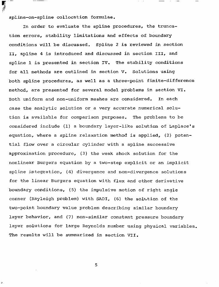
collocation formulae.

evaluate the spl ine procedures , the t runca-

t i o n e r r o r s , s t a b i l i t y l i m i t a t i o n s and effects of boundary

condi t ions w i l l be discussed. Spl ine 2 i s reviewed i n section

11, s p l i n e 4 i s introduced and discussed in sect ion 111, and

s p l i n e 1 i s presented i n s e c t i o n IV. The s t a b i l i t y c o n d i t i o n s

for a l l methods a r e o u t l i n e d i n s e c t i o n V. So lu t ions us ing

both spline procedures , as w e l l a s a t h ree -po in t f i n i t e -d i f f e rence

method, a r e p re sen ted fo r s eve ra l model problems i n s e c t i o n V I .

Both uniform and non-uniform meshes are considered. In each

c a s e t h e a n a l y t i c s o l u t i o n o r a very accurate numerical solu-

t i o n i s available for comparison purposes. The problems t o be

considered include (1) a boundary layer- l ike solut ion of Laplace 's

equation, where a s p l i n e r e l a x a t i o n method i s appl ied, ( 2 ) poten-

t i a l flow over a c i r cu la r cy l inde r w i th a sp l ine success ive

approximation procedure, ( 3 ) t h e weak shock solut ion for t h e

nonlinear Burgers equation by a two-step expl ic i t o r an imp l i c i t

s p l i n e i n t e g r a t i o n , (4 ) divergence and non-divergence so lu t ions

for the l inear Burgers equa t ion wi th f lux and o t h e r d e r i v a t i v e

boundary conditions, (5) the impulsive motion of r ight angle

corner (Rayleigh problem) with S A D I , ( 6 ) t he so lL t ion o f t he

two-point boundary value problem describing similar boundary

layer behavior, and ( 7 ) non-similar constant pressure boundary

layer so lu t ions for l a rge Reynolds number using physical var iables .

The r e s u l t s w i l l be summarized i n s ec t ion VII.

5

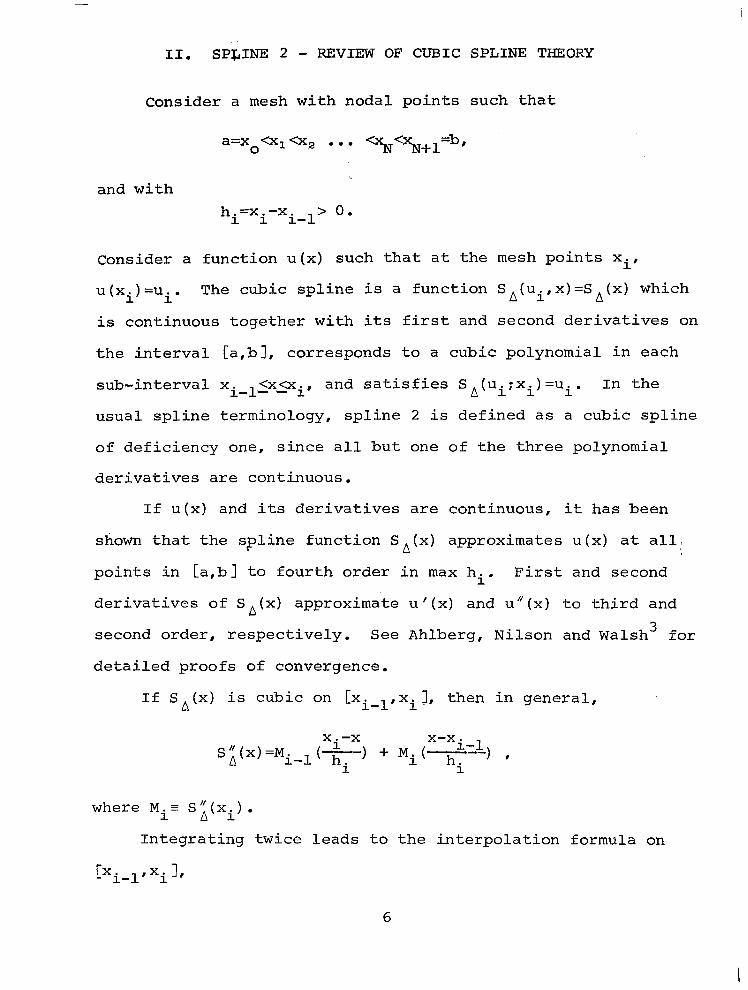
11. SP&INE 2 - REVIEW OF CUBIC SPLINE THEORY

Consider a mesh with nodal points such that

a=x oC,<x, . . . 0 <xN<xN+l=b'

and wi th

consider a func t ion u (x ) such t ha t a t t he mesh p o i n t s xi,

u ( x . ) =u The cub ic sp l ine i s a funct ion S (u x) =S (x) which 1 io A i' A

is continuous together with i t s f i r s t and second d e r i v a t i v e s on

the i n t e rva l [ a ,b ] , co r re sponds t o a cubic polynomial in each

sub-interval xi l z x s i , and s a t i s f i e s S (u - x . ) =u I n t h e

usua l sp l ine t e rminology, sp l ine 2 i s def ined as a cub ic sp l ine

o f de f i c i ency one , s ince a l l b u t one of the three polynomial

der iva t ives a re cont inuous .

A i' 1 i ' -

I f u ( x ) and i t s der iva t ives a re cont inuous , it has been

shown t h a t t h e s p l i n e f u n c t i o n S (x) approximates u(x) a t a l l ,

p o i n t s i n [ a , b ] t o f o u r t h o r d e r i n max hi. First and second

d e r i v a t i v e s of S (x) approximate u' (x) and u " ( x ) t o t h i r d and

A

n second order, respectively. See Ahlberg, Nilson and Walsh' f o r

detailed proofs of convergence.

If s (x) i s cubic on [xi l,xi 1, then in general , A - x "x i x-x

SI' (x ) =Mi (- ) + M. ("- , i-1) A - hi 1 hi

where M.= S/'(x ) . 1 A i

In tegra t ing twice l eads to the in te rpola t ion formula on

Lxi-l 8 xi 1 8

6

The cons tan ts of integrat ion have been

and S A (xim1) =uiml. s ,(x) on [xi, xi+l 1 rep lac ing i i n ( l a )

evaluated from S (x ) = u

i s obtained with i+l A i i

The unknown d e r i v a t i v e s Mi a r e r e l a t e d b y e n f o r c i n g t h e

cont inui ty condi t ion on- S '(x). With S '(x-)=rni on Ci-1, i] and

1, w e r e q u i r e my = rnz = m W e f i nd fo r A A i

s ' ( x . )=mi + + on [ X ~ , X ~ + ~ A 1 1 i'

i=l, . . .,N,

Addi t iona l sp l ine r e l a t ionsh ips t ha t a r e ea s i ly de r ived a r e

l i s t e d below:

m = - hi hi u -u Mi+ - + i i-1 .

i 3 6 Mi-l '2 I

3 ( u p ) i-1 hf I

+ -

7

I

2 m i - l 4mi u -u Mi - + - -6 - i i-1 .

hi hi hf I

Eqs. ( lb ) o r (IC) l e a d t o a system of N equa t ions fo r t he N+2

unknowns Mi o r m r e spec t ive ly . The a d d i t i o n a l two equat ions

a re ob ta ined from boundary conditions on mot %+1 o r M

i'

0' %+1 The resu l t ing t r id iagonal sys tem for Mi o r m i s diagonal ly

dominant and solved by an e f f i c i en t i nve r s ion a lgo r i thm . Spl ine 2 fo r So lv inq Pa r t i a l D i f f e ren t i a l Equa t ions l - 8

i 3

I f t h e v a l u e s ui a r e no t p re sc r ibed bu t r ep resen t t he so lu -

t i on o f a quas i - l i nea r s econd o rde r pa r t i a l d i f f e ren t i a l equa-

t i o n , u = f ( u 8 u u ) , then an approximate solution for ui can t x, xx

be obtained by cons ide r ing t he so lu t ion o f

This formulation i s des igna ted sp l ine 2 . I f t h e time d e r i v a t i v e

i s d i s c r e t i z e d i n a s imple f in i te -d i f fe rence fash ion , w e have

U n+l-un i = ( l - e ) fn+ef n + l

A t I

e=o, e x p l i c i t ; 8=1, i m p l i c i t ; e+# Crank-Nicolson. For the

e x p l i c i t i n t e g r a t i o n t h e s t a b i l i t y l i m i t a t i o n s a r e q u i t e s e v e r e ,

see Refs. 1 ' 2 and sec t ion V I . Therefore a two-step procedure i s

considered and i s given as:

8

U n+l-.p S tep 2: i i -n+l

A t = f

Example:

Consider the l inear Burgers equat ion

With ( lb) and (IC) w e ob ta in a system of 3N equat ions for

3-(N+2) unknowns (see R e f s . ' 1 8 2 f o r f u r t h e r d e t a i l s on t h e

de r iva t ion ) . The system ( 2 ) can be w r i t t e n a s t

where

A .= -l/hi 0

3/h: l /hi 0

53 a1 %! B . = 1 [ ( l + l / o ) / h i 0 ( ~ + l ) hi/3 :

-3 ( l - l / o a ) /ha 2 ( l+l/~) /hi 0 1 i

0

0

hi+l 1

* It i s poss ib l e t o t r e a t t h e v i s c o u s terms (Mi) i m p l i c i t l y (8=1) and the convect ion terms e x p l i c i t l y . A s shown i n R e f s . 1,2, t h e s t a b i l i t y o f t h e t w o - s t e p p r o c e d u r e fior viscous f lows i s improved.

r e l a t i o n s (1) .

"

'A number of v a r i a t i o n s on t h i s system can be der ived wi th the

9

P, P I .i=[ 0 0 E] ;

0 0 0

0 0 E.=[ 1 0 0

0 0 0

v.=[u m M ~ I J.

1 i' i'

and

A s ign i f i can t advan tage o f t he sp l ine 2 formulation is t h a t w i t h

expressions (1) it i s p o s s i b l e t o r e d u c e t h e 3x3 matrix system

( 3 ) t o a s c a l a r s e t of equat ions for M alone. The d e t a i l s o f

t h i s r educ t ion p rocess a r e found i n Refs. 1'2. j

For equations with two space dimensions such that u = f ( u 8 u

) a s p l i n e a l t e r n a t i n g d i r e c t i o n i m p l i c i t (SADI) t X'

uy' uxx' uyy procedure has been presented by Rubin and Graves'' '. A s p l i n e

successive approximation method can a lso be simply formulated.

Both techniques are discussed la ter i n th i s paper where severa l

example problems are p resented .

Truncation Error ""- For i n t e r i o r p o i n t s , t h e s p a t i a l a c c u r a c y o f t h e s p l i n e

approximation can be d i r ec t ly e s t ima ted from the formulas ( l b )

10

and ( le ) or ( I f ) . Expanding mi, M . and ui in Taylor series

and assuming the necessary cont inui ty o f der iva t ives for u (x#y)#

1

we obta in , wi th ~ h ~ + ~ / h ~ ,

('xx 1 ) .=Mi+ (uiv) ihf ( a3+l) /12 (o+l)

- (uV) ih: ( 0-1) ( 2 u2+5 ~-t -2) /180

-(uvi) .h~Ca2/360+(u-1)2(7~2-2a+7) /10801 1 1

and

(ux)i=m.+(u 1 i v )ih:u(o-1)/24 + t

+(uv) a [ l+a(a- l ) ]/180 + 0 (hz) .

Fyf e lo has presen ted s imi l a r r e l a t ions ,

fo r cons t an t hi, i n h i s co l loca t ion ana lys i s o f cub ic sp l ines

fo r t he so lu t ion o f two point boundary value problems.

Therefore , the spl ine approximation with a non-uniform mesh

i s second-order accurate for Mi and th i rd -o rde r fo r mi. For a

uniform mesh m becomes fourth-order with Mi remaining second-

order accura te . In the next sec t ion a f in i te -d i f fe rence expres-

s ion f o r (uiv) i s used t o increase the accuracy of Mi and hence

i

the overal l accuracy of the procedure. With this modif icat ion

th i s fo rmula t ion w i l l be termed spl ine 4.

'If (IC) i s used t o e v a l u a t e t h e t r u n c a t i o n error f o r mi, t h e cons tan t 24 i n t h e second expression on the r ight-hand s ide becomes 7 2 . For the uniform case, (4b) i s recovered i n a l l cases.

11

111. SPLINE 4 - DERIVATION AND DISCUSSION

In o rde r t o improve the overa l l accuracy of the s p l i n e 2

formulation, it i s necessary t o reduce the order of the t runca-

t i o n e r r o r f o r ( u ) i n ( 4 a ) . Although a nunher of procedures

a re poss ib l e , w e have chosen a very simple modification, whereby xx i

the e r r o r term i n ( 4 a ) f o r (uiv) i s approximated by a three-

p o i n t d i s c r e t i z a t i o n f o r Mi. This approximation i s f i r s t - o r d e r

accura te w i t h a non-uniform mesh and second-order w i t h a uniform

mesh. Therefore the spl ine approximation for (u ) i s improved,

and p a r a l l e l s t h a t for (uX).; i.e., third-order accuracy i s

achieved for a non-uniform grid and fourth-order accuracy for

xx i

uniform mesh. This improvement l e a d s t o what i s termed s p l i n e

8

where A= (1+a3)/a(1+a) . The fami l ia r th ree-poin t d i scre t iza t ion formula i s

1 2

Therefore, (4a) or (sa) becomes

) 1 . =Mi+ ( A / 6 ) ( Mi+l- (1+ a) Mi+ dli - 1> -7hT(1+02) (0-1) (uv) i/180-hf(uvi) [aa/360

With (4b) ,

(ux) i=mi+O (( 0-1) h9, h4) t

and w e ob ta in a uniform higher-order approximation termed

sp l ine 4 . When ~ l , s p l i n e 4 i s fourth-order accurate and t h e

t runca t ion e r ror o f (5b) i s smaller than that obtained with

Hermitian or Pad6 gnethods5-’, which are in turn smaller

than the error obtained witn five-point finite-different

$

discretizations.

I n t h e s p l i n e 4 p rocedure t he r e l a t ions ( l b - lh ) still apply;

however, the interpolat ion polynomial i s no longer appl icable as

spline 4 represents a hig,her-order interpolation. The governing s y s t e m

‘It i s poss ib l e t o app ly (5b ) t o (4b ) t o make (ux) fourth-order

*Higher-order procedures, e.g., spline 6, can be der ived i n a

even with a non-uniform mesh.

s i m i l a r manner , and s p l i n e 2 i s recovered from spline 4 wi th A set equal t o zero.

13

remains t r id iagonal . Unl ike sp l ine 2, where the system can be

reduced t o t h a t f o r M, alone, the appearance of off-diagonal I

terms i n (5b) restricts t h e

system i n ( u ~ , M ~ ) .

For the l inear Burgers

t h e form (3b) wi th

r educ t ion p rocess t o a 2x2

equation the system i s s t i l l of

A l l o t h e r e n t r i e s i n ( 3 c 8 3 d ) a r e unchanged.

I V . FINITE-DIFFERENCE THEORY/SPLINE 1

If the procedures given previously for s p l i n e 2 and s p l i n e 4

a re r epea ted fo r a quadra t ic po lynomia l in te rpola t ion wi th both

der iva t ives cont inuous (a quadra t ic sp l ine o f zero def ic iency) ,

we f i nd on [xi - 1 8 xi],

S A (x )=u . 1 (x-x i-1 )/h+ui,l(xi-x)/h+(ui-ui-l-hm.) 1 (x-xi - 1) (xi-x)/ha,

where

s A 1 (X.)’Ui, sA(xi-l)=ui-l, S A ’ (xi) =mi,

and - Mi = S ” ( x . ) = - 2(ui-u -m.h)/h“ . A 1 i-1 1

-

14

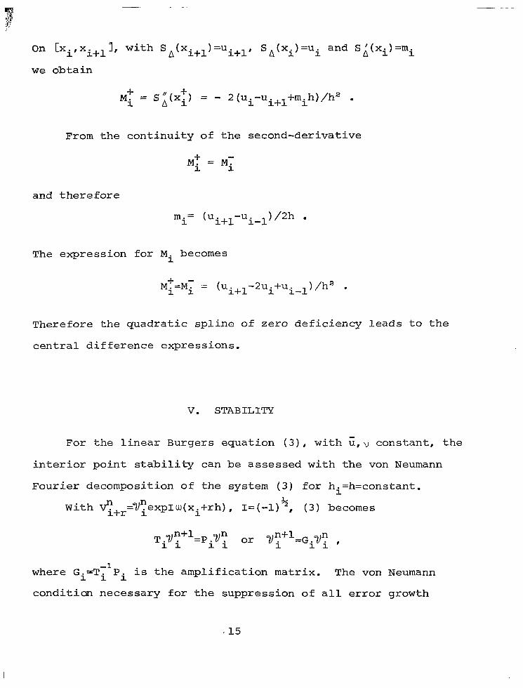
O n C X ~ , X ~ + ~ ~ , w i th s A S A 1 (x . )=u i and S ' ( x A i )=mi

w e ob ta in

" = S " ( X . ) = - 2(ui-u +mih)/h2 . 3. Mi A 1 i+l

From t h e c o n t i n u i t y of the second-derivat ive

Mi + - - Mi -

and t h e r e f o r e

The express ion for Mi becomes

M. + =M- = ( U ~ + ~ - ~ U . +u ) /h2 . 1 i 1 i-1

There fo re t he quadra t i c sp l ine of z e r o d e f i c i e n c y l e a d s t o t h e

cent ra l d i f fe rence express ions .

V. STABILITY

For t h e l inear Burgers equat ion (3), w i t h u , v constant , t h e

i n t e r i o r p o i n t s t a b i l i t y can be assessed w i t h t h e von Neumann

Fourier decomposition of the system ( 3 ) for h .=h=constant . 1

With q+r=vrexpIw(xi+rh), I=(-1) + , ( 3 ) becomes

where Gi=TflPi i s the ampl i f ica t ion mat r ix . The von Neumann

condi t ian necessary for the suppress ion of a l l e r r o r growth

r e q u i r e s t h a t t h e s p e c t r a l r a d i u s p ( G i ) l . The eigenvalues of

G. a r e X 1 io

For the one-dimensional equation ( 3 ) , t h r e e numerical pro-

cedures were considered: (1) convection (mi) and d i f f u s i o n (Mi)

explicit , (ii) convec t ion exp l i c i t , d i f fus ion implicit (two

s t e p s r e q u i r e d f o r i n v i s c i d s t a b i l i t y ) , and (iii) d i f f u s i o n and

convect ion implici t . With expl ic i t convect ion, (i) o r (ii) ,

both divergence and nondivergence forms of the equations have

been evaluated i n R e f s . 1 and 2.

The s t a b i l i t y c o n d i t i o n s imposed on t h e s e schemes i s determ-

ined from

lh, l 5 1

(i) Expl ic i t convec t ion and d i f fus ion : 0=0 i n (2a,3) .

limits a r e

These r e s u l t s a r e more r e s t r i c t i v e t h a n t h e limits found f o r t h e

forward time cen t r a l space exp l i c i t f i n i t e -d i f f e rence method

o r s p l i n e 1, which a r e

12

1 6

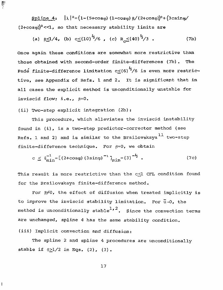
Spline 4: I X [ 2= (1- (S+cosep) (l-coscp) e/ (2+cos~p))~+ (3csind (2+c0scp))~<<l, so that necessary stability limits are

(a) e,51/48 (b) CZ(l0) 2/6 8 (C) R <(40) '/3 . k C- (7b)

Once again these conditions are somewhat more restrictive than

those obtained with second-order finite-differences (7b). The

Pad; finite-difference limitation cL(6) 2/6 is even more restric-

tive, see Appendix of Refs. 1 and 2. It is significant that in

all cases the explicit method is unconditionally unstable for

inviscid flow: i.e., p=O.

k

(ii) Two-step explicit integration (2b) :

This procedure, which alleviates the inviscid instability

found in (i), is a two-step predictor-corrector method (see

Refs. 1 and 2) and is similar to the Brailovskaya" two-step

finite-difference technique. For p=O, we obtain

This result is more restrictive than the ccl CFL condition found

for the Brailovskaya finite-difference method.

For p#O, the effect of diffusion when treated implicitly is

to improve the inviscid stability limitation. For E-0, the

method is unconditionally stable', '. Since the convection terms

are unchanged, spline 4 has the same stability condition.

17

I

( i v ) SADI :

In Ref. 1, t h e i n t e r i o r p o i n t s t a b i l i t y a n a l y s i s i s extended

t o t h e two-dimensional SADI procedure ; uncondi t iona l s tab i l i ty

i s demonstrated.

Al though the impl ic i t p rocedures l ead to uncondi t iona l ly

s t ab le fo rmula t ions , a s w i th f i n i t e -d i f f e rence methods, t h e tri-

diagonal system may no t be diagonal ly dominant . In this case

the invers ion a lgor i thm3 may l e a d t o l a r g e e r r o r growth. Diag-

onal dominance can be achieved by a sp l ine adap ta t ion o f t he

f ini te-difference procedure given in Ref . 12. For a l l t h e

problems t reated here this modif icat ion i s unnecessary. In other

app l i ca t ions it w i l l p l ay a s i g n i f i c a n t r o l e i f a c c u r a t e s o l u -

t i o n s a r e t o be obtained.

V I . RESULTS

Several model problems have been cons ide red i n o rde r t o

eva lua te t h e cub ic sp l ine co l loca t ion methods presented herein.

For each of these problems an analyt ic solut ion or re l iable

numerical solution i s available for comparison purposes. Spline

i n t e r p o l a t i o n ( s p l i n e 2 and s p l i n e 4) i s used t o approximate the

spat ia l gradients . For the one-dimensional Burgers equat ion the

in tegra t ion procedure ou t l ined in Sec t ion I1 i s adopted. Implici t

or two-step explicit methods are used. For the two-dimensional

d i f fus ion equat ion , so lu t ions a re ob ta ined wi th the S A D I formula-

t i o n . The Laplace equation in Cartesian and polar coord ina tes

i s evaluated with a spline successive approximation procedure.

F ina l ly , t he s imi l a r i t y equa t ions fo r t he f l a t p l a t e boundary - l aye r

18

and t h e two-dimensional s tagnat ion point are solved by direct

integration of the result ing two-point boundary value problems.

Solutions are obtained with both uniform and non-uniform

meshes. Three-point f ini te-difference calculat ions are included

i n o r d e r t o a s s e s s t h e r e l a t i v e i n c r e a s e i n accuracy associated

with the higher-order procedures. The r e s u l t s a r e p r e s e n t e d i n

t a b u l a r form so that meaningful comparisons are possible.

A . Burgers Equation

The nonl inear Burgers equat ion (3a) , wi th x=x, u=u(z, t ) "

and x=;;- (1 /2 ) t, becomes

ut+(u-1/2)ux=VUxx (8a)

w i t h w constant and the boundary conditions

u-l a s x+ "00 and 1.140 a s x-90 . (ab)

The s t e a d y s t a t e s o l u t i o n of (8a) i s

Spl ine 2 and the f i n i t e -d i f f e rence so lu t ions o f (8) have

been discussed in Refs. 1 and 2 . Both implicit and two-step

exp l i c i t i n t eg ra t ion t echn iques , a s ou t l i ned i n Sect ion 11,

have been applied successfully182. Spline 4 solut ions have now

been obtained with the implici t and/or two-step procedures of

( 2 a ) , ( 2 b ) . The sys tem (3) wi th the coef f ic ien ts ( 6 ) a r e con-

s idered . In t h e a c t u a l c a l c u l a t i o n s t h e 3x3 system ( 3 ) i s

*

*

* The n o n l i n e a r c o e f f i c i e n t u i s t r e a t e d i t e r a t i v e l y o r w i t h quas i - l i nea r i za t ion l r2 .

I

19

reduced t o a 2x2 system. mi i n Vi i s el iminated with ( le) or

(If) . The boundary conditions (8b) on u l , %+1 a r e s p e c i f i e d

a t x=xmax, w i t h xma&3. The boundary conditions on Mi a r e ob-

t a ined from t h e t h i r d - o r d e r a c c u r a t e r e l a t i o n

(a) (uxx) 1= (uxx) a- (M,-M1)

With (uxx) evaluated from (5c), we ob ta in

where ~ h , / h , . From the governing equat ion (8a) ,

(uxx) 1= (ux) 1/2 w=m& w

so t h a t w i t h ( l f ) ,

m,=-h2M,/3-h2M,/6 + (u2- l ) /h2

and (9b) becomes

M, (2vt~~A/3+h,/3)+M,(h,/6-~(1+0) A/3)+(vA/3)M,-u2/h,=-l/h2.

(9c)

(b) An a l t e r n a t e form of ( 9 a ) , r e l a t i n g o n l y t h e t w o po in t s ,

i=l and i = 2 , can be derived by evaluating (uxx) a from ( 8 a ) . The

tempora l d i scre t iza t ion i s given by (2a) . W e ob ta in

#+" + a Mn+l + a3u2 a1 1 2 2 = a4 (9d) l-i+l

20

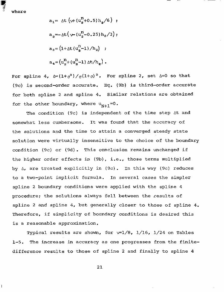
al= A t (vt(ut+0.5)h2/6) :

a3= (I+ A t (uz-1)/h2) :

For sp l ine 4, A = ( l + ~ ~ ) / ~ ( l + ( y ) ~ . For s p l i n e 2, set A=O so t h a t

(9c) i s second-order accurate. Eq. (9b) i s th i rd-order accura te

f o r b o t h s p l i n e 2 and s p l i n e 4. S imi l a r r e l a t ions a r e ob ta ined

for the other boundary, where U ~ + ~ = O .

The condi t ion (9c) i s independent of t h e time s t e p A t and

somewhat less cumbersome. I t was found tha t the accuracy of

t h e s o l u t i o n s and t h e time t o a t t a i n a converged s teady s ta te

s o l u t i o n w e r e v i r tua l ly i n sens i t i ve t o t he cho ice o f t he boundary

condi t ion (9c) or (9d) . This conclusion remains unchanged i f

t h e h i g h e r o r d e r e f f e c t s i n ( 9 b ) , i.e., those terms mul t ip l ied

by A , a r e t r e a t e d e x p l i c i t l y i n (9c) . I n t h i s way (9c) reduces

t o a two-point implicit formula. I n severa l cases the s impler

s p l i n e 2 boundary conditions were app l i ed w i th t he sp l ine 4

procedure: the solut ions a lways f e l l be tween the resu l t s of

s p l i n e 2 and s p l i n e 48 bu t gene ra l ly c lose r t o those o f sp l ine 4.

Therefore , i f s implici ty of boundary condi t ions i s d e s i r e d t h i s

i s a reasonable approximation.

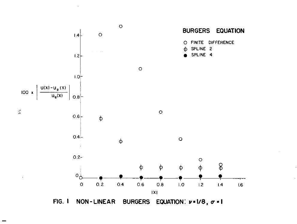
T y p i c a l r e s u l t s a r e shown, f o r w=1/8, 1/16, 1/24 on Tables

1-5. The inc rease i n accuracy as one progresses from t h e f i n i t e -

d i f f e r e n c e r e s u l t s t o those o f sp l ine 2 and f i n a l l y t o s p l i n e 4

21

i s apparent . This i s p a r t i c u l a r l y t r u e w i t h t h e non-uniform

meshes of Tables 2 and 3 . For the condi t ions of Table 3, the

f i n i t e - d i f f e r e n c e c a l c u l a t i o n s w i t h the two-step expl ic i t pro-

cedure did not converge. An osc i l l a to ry behav io r was observed

a f t e r 3200 i t e r a t i o n s . I n c e r t a i n c a s e s , where hi i s r e l a t i v e l y

l a rge , t he nature of the t runca t ion errors (4a84b) of s p l i n e 2

and s p l i n e 4 i s such t h a t a loca l va lue ob ta ined w i t h s p l i n e 2

may be a s a c c u r a t e o r more accura te than tha t ob ta ined w i t h

s p l i n e 4. These are except ional cases , however, and never occur

f o r hi<.cl. A percen tage e r ro r p lo t fo r the r e s u l t s of Table 1

i s shown on Figure 1. ue(x) denotes t h e exac t so lu t ion (8c) .

So lu t ions fo r o the r v va lues a r e of a s i m i l a r n a t u r e and

therefore have not been included here.

B. Linear Burgers Equation

Consider t h e equation

u +vuxx=O , . on 0 , o c ~ l X

w i t h boundary conditions u (1)=1 and on x=08 vux+u=O. The exac t

solution is ue(x)=exp(l-x)/v. In some unpublished work by

George J. Fix", it was shown that with this flux boundary

condition linear finite element theory naturally satisfies the

required conservation condition at the boundary and therefore

leads to more accurate solutions than obtained with non-divergence

versions of spline 2 or conventional finite-difference theory.

If finite-difference theory is developed in divergence or

conservation form, the resulting equations are identical with

*Institute for Computer Applications in Science and Engineering

22

those of the l inear , second-order accurate , f ini te element '

method. I f s p l i n e 2 i s recast in divergence form the solut ions

are considerably more accurate than the non-conservation r e s u l t s

and a l s o improve upon the conse rva t ion f i n i t e e l emen t ( f i n i t e -

difference) calculat ions. Therefore , wi th the f lux boundary

condi t ion it appears that d ivergence form may be r e q u i r e d i f

a c c u r a t e s p l i n e s o l u t i o n s a r e t o be obtained. On t h e o t h e r

hand, i f a modified derivative boundary condition was considered

i n l i e u o f t h e f l u x c o n d i t i o n , t h e s e n s i t i v i t y t o divergence 2orm

was no longer apparent . It i s p o s s i b l e t h e r e f o r e t h a t t h e f l u x

cond i t ion r ep resen t s a s ingular case.

The governing systems of equations and the boundary condi-

t i ons fo r t he d i f f e ren t fo rmula t ions a r e a s follows:

Finite-Difference/Non-Divergence Form

v ( U i + l + U i - l - 2 ~ . 1 ) /h + ( u ~ + ~ - u ~ - ~ ) /2 = 0 ( l o a )

El iminat ing uml from ( 1 O c ) wi th t he d i f f e rence equa t ion ( l oa ) ,

23

I

The governing equation ( l l a ) i s i d e n t i c a l w i t h the non-divergence

equat ion ( loa) . The a l t e r a t i o n s a p p e a r i n the boundary conditions

A t x=l , u =1 N

A t x=08 ( vux+u) = 0. Therefore, %

The boundary condition ( l l b ) d i f fe rs from t h e non-divergence

condi t ion (LOd) . Spl ine 2/Non-Diverqence Form

The governing equation (12a) i s combined

w i t h the s p l i n e r e l a t i o n s (1). The boundary conditions are

8 vmo+uo = 0 . (12b)

Spline 2/Diverqence Form

The governing equation (13a) i s combined

(vm+u) i+l= (vm+u) i.l ( 1 3 4

w i t h the s p l i n e r e l a t i o n ( IC) . The boundary conditions are

u =1 N

and vmo+uo+a( vm, +u, ) = 0 ,

where a=O corresponds to the exact boundary value and

a=l corresponds t o an averaged boundary condition.

24

The r e s u l t s o f t h e s e c a l c u l a t i o n s a r e shown on Table 6.

It i s seen that the non-conservation (NC) so lu t ions w i th t en

mesh p o i n t s (N=10) a re r a the r poor when compared w i t h e i t h e r

t h e f i n i t e element o r spline 2 conservation (C) so lu t ions . I t

i s s i g n i f i c a n t t h a t t h e s p l i n e d i v e r g e n c e s o l u t i o n s , f o r b o t h

a=O and a=l, are considerable improvements over the f ini te-

e lement resu l t s . A s t h e nuniber of mesh p o i n t s i n c r e a s e s t h e

non-divergence solutions do show some improvement, w i th sp l ine 2

more a c c u r a t e t h a n f i n i t e - d i f f e r e n c e s , b u t t h e s e r e s u l t s a r e

still less accura te than f in i te -e lement so lu t ions . The t e n po in t

s p l i n e 2 divergence form a=l so lu t ions a r e abou t a s accu ra t e a s

t h e 50 p o i n t f i n i t e e l e m e n t r e s u l t s .

Also shown on t h e t a b l e a r e t e n po in t so lu t ions w i th some-

what modi f ied der iva t ive condi t ions a t x=O. The exac t so lu t ion

i s unchanged. These derivative boundary conditions were treated

i n much t h e same manner a s t he f l ux cond i t ion fo r each of t h e

procedures . For the f ini te-element solut ions an average condi t ion

was app l i ed . S ign i f i can t ly t he l a rqe d i f f e rences between diverq-

ence so lu t ions no lonqer occur. The sp l ine so lu t ions a re a lways

t h e most accurate , wi th a small increase i n accuracy when diverg-

ence form i s assumed.

C. Linear Corner F l o w

The two-dimensional diffusion equation

*

w i t h t h e i n i t i a l c o n d i t i o n u ( o # x # y ) = o and boundary conditions

25

has the exac t so lu t ion

u=l-erf X e r f Y ,

where X = X ( R /t) 5 8 y = 5 ( R e / t ) % . 1

2 e

This solution describes the impulsive motion of a r i g h t -

angled corner formed by two i n f i n i t e f l a t p l a t e s and r e s u l t s o f

t h e SADI s p l i n e 2 ca lcu la t ion have been presented in Refs . l , 2 .

The S A D I procedure for the diffusion equat ion (14a) for both

s p l i n e 2 and s p l i n e 4 i s given as follows:

S tep 1:

Step 2:

where

and

Lij and

(lb) .

n+% - n n++ i j +(“YY 1 7 i j U - u + ((uxx) i j > n .) A t / ( 2 R e ) ( 1 5 4

n+l U i j = u n-& i j + ((uXx) n++ i j + (uYy) :;’) At / (2Re) ( 1 5 ~

(‘xx ) i j - - M. 17 .+(Ax/6) (Mi+l, j - ( l + O x ) M . 17 .+o x M i-l#-~ * ) . (1-1

(u yy 1 ij- - Lij+(Ay/6) ( L i , j + l - ( l + o ) L . .+OYLi, j-l Y 1 3 ) (16b)

Mi j each s a t i s fy a t r i d i agona l equa t ion o f t he form

*X

OX

= ( l + ~ ~ ~ ) / o ~ ( l + ~ ~ ) ; A = ( l+a3) /a ( 1 + 0 ~ ) ~ Y Y Y

= hi+l/hi ; u = k /k ; h . = x . -X ; k .=y .-y Y j+ l j 1 1 i-1 3 7 j-1.

The s p l i n e 2 formulation i s recovered with A = A =O. The boundary

cond i t ions fo r u are given by (14b). The boundary conditions X Y

i

26

f o r Lij,Mij are obtained from (16) with (uxx)ij= (u,) i j=O on

the boundar ies , o r from (9a) with (uxx) i+l, obtained from (14a) . * The s o l u t i o n f o r step 1 is ob ta ined w i th t he t r i d i agona l

2x2 system for M i j

s imi la r p rocedure for Li j , ui j i s r e q u i r e d f o r s t e p 2 . and uij as descr ibed by (15a) and (lb) . A

The s o l u t i o n f o r R e = l O O O is given on Table 7. A non-uniform

21x21 mesh wi th 0 =cr =1,5 was prescr ibed , The step s i z e At=0.01.

The s o l u t i o n i s shown for t=2.0. All o f t h e s o l u t i o n s a r e X Y

reasonably good fo r t h i s ca se , bu t once aga in t he spline s o l u t i o n s

a r e somewhat bet ter .

D . Laplace Equation

The Laplace equation

u +u = 0 ; u=u(x,y) , xx YY ( 1 7 4

w i t h the boundary conditions u(O,y)=u(l ,Y)=O; u(x,O)=sinnx;

lim ydm u (x,y)=O

* This procedure has been demonstrated for the Burgers equation by the d i scuss ion lead ing t o (9d) .

27

I II

Using the genera l express ion for second der iva t ives (16),

Eq. (17a) can be p u t i n t o a s p l i n e form. With t h e t r i d i a g o n a l

r e l a t i o n s h i p f o r L i j and Mij (lb), t h i s l e a d s t o a 3x3 system

fo r t he vec to r Vij a t a l l i n t e r i o r mesh poin ts :

‘i-jVi8j-1 +B i j V . 11 .+CijVi, j+l+DijVi-l, j+Eij V i+l, j- - 0 (18)

0

uyAy’6 li 1

0 0 0

6 1+ ax 7 - h i ‘x

Ay/6

3F y j

-6 0 Y

0 0

2 ( l + a ) Y

0

0

0 1 , 28

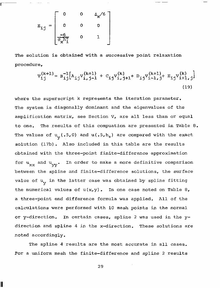
The so lu t ion i s obta ined wi th a success ive po in t r e l axa t ion

procedure,

where t h e s u p e r s c r i p t k r ep resen t s t he i t e r a t ion pa rame te r .

The system i s diagonally dominant and the eigenvalues of the

amplif icat ion matr ix , see Sect ion V, a r e a l l less than or equal

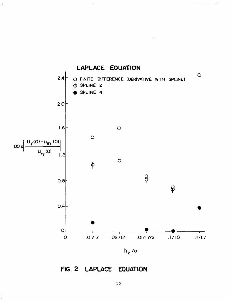
t o one. The r e s u l t s o f t h i s compuation a re p resented in Table 8.

The values of u ( - 5 , 0) and u ( - 5 , h a ) a r e compared w i t h t he exac t

so lu t ion (17b). Also inc luded in t h i s t a b l e a r e t h e r e s u l t s

ob ta ined wi th the th ree-poin t f in i te -d i f fe rence approximat ion

f o r u and u I n o r d e r t o make a more def ini t ive comparison

between t h e s p l i n e and f in i t e -d i f f e rence so lu t ions , t he su r f ace

value of u i n t h e l a t t e r c a s e was ob ta ined by sp l ine f i t t i ng

the numerical values of u(x,y) . I n one case noted on Table 8,

a three-point end difference formula was appl ied. All of the

c a l c u l a t i o n s were performed with 10 mesh p o i n t s i n t h e normal

o r y -d i r ec t ion . In ce r t a in ca ses , sp l ine 2 was used i n t h e y-

d i r e c t i o n and s p l i n e 4 i n t h e x-direct ion. These solut ions are

noted accordingly.

Y

xx YY-

Y

The s p l i n e 4 r e s u l t s a r e t h e most a c c u r a t e i n a l l c a s e s .

For a uniform mesh t h e f i n i t e - d i f f e r e n c e and s p l i n e 2 r e s u l t s

29

are o f equa l accuracy as there a re no convec t ion e f fec ts in the

problem. Moreover, i f t h e s p l i n e 2 and the f i n i t e - d i f f e r e n c e

so lu t ions a re averaged , the spline 4 r e s u l t s a r e c l o s e l y approx-

imated. For a non-uniform mesh t h e improved accuracy of spline 2

over the f ini te-difference approximation i s now apparent.

The s p l i n e 4 resu l t s a re remarkably accura te wi th ~ 1 . 7 ,

h,=0.1 and ~ ~ ~ ~ " 2 8 . 6 6 . For t h i s mesh the re a r e on ly fou r po in t s

i n the reg ion 0 3 < l - a s compared wi th a uniform mesh (h=0.1) and

t e n p o i n t s . The coarse mesh, s p l i n e 4 r e s u l t s a r e more accu ra t e

than the uniform mesh f i n i t e - d i f f e r e n c e s o l u t i o n s .

The 1.7/.2 n o t a t i o n f o r o means t h a t ~ 1 . 7 for h.<0.2. 1

For h.>0.2, u becomes un i ty . I n t h i s way t h e mesh width does

not exceed a spec i f i ed maximum value. This type of mesh alignment 1-

i s u s e f u l i n boundary layer problems, where a f i n e g r i d i s d e s i r e d

near the surface, and a uniform but coarser mesh i s r equ i r ed i n

the ou ter inv isc id reg ions . This p rocedure i s a l so app l i ed fo r

the boundary layer solut ions i n Sect ion V1.F. An e r r o r p l o t i s

given on Figure 2 .

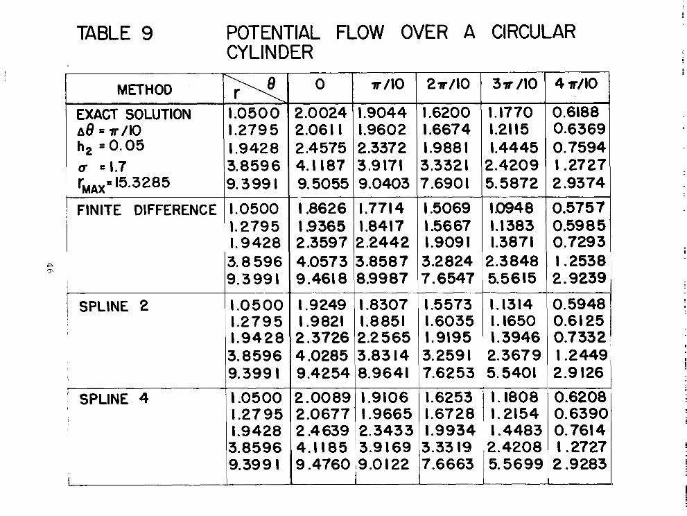
E. P o t e n t i a l Flow Over a Circular Cylinder

The govern ing equat ion in cy l indr ica l coord ina tes for the

potent ia l f low over a c i r c u l a r c y l i n d e r i s given by

1 1

u + k u + + - u = o rr r r r 8 8 . The boundary condi t ions are ur( l , 8 ) = 0 and l i m u ( r , 8)-trcos8. The

exac t so lu t ion of Eq. ( 2 0 ) with these boundary conditions i s r-m

... .

u=(r+r)cos8 . E q s . (17a) and (20) differ only by the appearance I

30

of the ur term which i s d i s c r e t i z e d b y t h e r e l a t i o n s ( l e ) or

( I f ) . The r e s u l t i n g 3x3 system for uij , L i j and M i j i s of t h e

form (19) . The coe f f i c i en t ma t r i ces i n t he p re sen t ca se w i l l

be somewhat a l t e r e d b y t h e ur t e r m .

The r e s u l t s of t h e i t e r a t i v e s o l u t i o n a r e p r e s e n t e d i n

Tables 9-11. A s in the p rev ious examples , the f in i te -d i f fe rence

so lu t ions a re ob ta ined by us ing th ree-poin t cen t ra l d i f fe rence

formulas. In Table 11, t h e s l i p v e l o c i t y on t h e f o r e s u r f a c e

of the cy l inder i s presented. The supe r io r i ty o f t he sp l ine

so lu t ions ove r t hose r e su l t i ng from f i n i t e - d i f f e r e n c e d i s c r e t i z a -

t i o n i s evident . It should be n o t e d t h a t t h e s l i p v e l o c i t y i n

t he f i n i t e -d i f f e rence ca se i s obtained by using a three-point

cen t ra l d i f fe rence formula , w h i l e t h e s p l i n e s o l u t i o n s r e q u i r e

only the two-point formula ( l e ) . The higher accuracy of the

two-point spl ine formula over the three-point f ini te-difference

re la t ions can be of considerable importance for problems with

derivative boundary conditions.

F. S i m i l a r i t y Boundary Layers

The boundary layer equat ions for the f low over a f l a t p l a t e

(p=O) and the two-dimensional stagnation point ( p = l ) can be

reduced t o the fo l lowing ord inary d i f fe ren t ia l sys tem by us ing

appropr ia te s imi la r i ty t ransformat ions , 1 4 .

f ’ = u ( 2 1 b )

The boundary conditions are

31

I n the s p l i n e 2 and s p l i n e 4 formulation, Eq. (21a) i s re-

duced t o a 2x2 system for ui and Mi and the two-point boundary

value problem i s solved subject t o (21c). For t h e first-order

equation ( 2 1 b ) , we ob ta in the following spline approximation

from (If) :

fi+l=fi+hi+lui+ 7 h!+l (MFi+.5MF 1 i+l ( 2 2

where MFi=(u’) f o r s p l i n e 2. For sp l ine 4, the fol lowing

r e l a t i o n t o e v a l u a t e MFi i s eas i ly de r ived from ( le ) and ( I f ) :

MFo= (u ’1 . E q s . ( 2 2 ) and ( 2 3 ) g ive rise t o an i n i t i a l v a l u e problem for f i

and MFi which i s solved by a marching procedure. Eq. ( 2 2 )

l eads to th i rd-order accura te express ion for f - t h e r e f o r e , f o r

non-uniform meshes and th i rd-order accura te so lu t ions , t h i s

i ‘

approximation i s adequate even for s p l i n e 4. For t h e f i n i t e -

d i f f e rence so lu t ions , a second-order accurate two-point formula

f o r f i , which i s cons i s t en t w i t h the accuracy of the o v e r a l l

scheme,is obtained w i t h t h e t r a p e z o i d a l r u l e . For p=1, the

nonl inear term u2 i s treated by quas i l i nea r i za t ion so t h a t

( U k + l ) . k i s the i te ra t ion parameter .

32

The resu l t s o f these computa t ions for both uniform as

w e l l a s non-uniform meshes a re t abu la t ed i n Tab le s 12-16. The

shear a t t h e w a l l i s propor t iona l t o f " ( o ) a n d t h i s term has

been eva lua ted for a v a r i e t y of meshes. The r e s u l t s a r e g i v e n

on Tables 1 5 and 16 f o r p=O and @=1, r e spec t ive ly . F in i t e -

d i f f e r e n c e s o l u t i o n s f o r ui a re ob ta ined by us ing the th ree-

po in t cen t ra l d i f fe rence approximat ion .

A s noted prev ious ly , the no ta t ion 0=1.8/1 means t h a t ~ 1 . 8

u n t i l hi reaches 1.0, a t which point ~1.0. h, i s t h e f i r s t .

mesh wid th o f f t he wa l l x=O; N i s t h e t o t a l number of mesh

p o i n t s , N6 is the nunher of mesh poin ts in the boundary l ayer

defined by xs6. A t x=6, ~ u - l , O ~ d O - s .

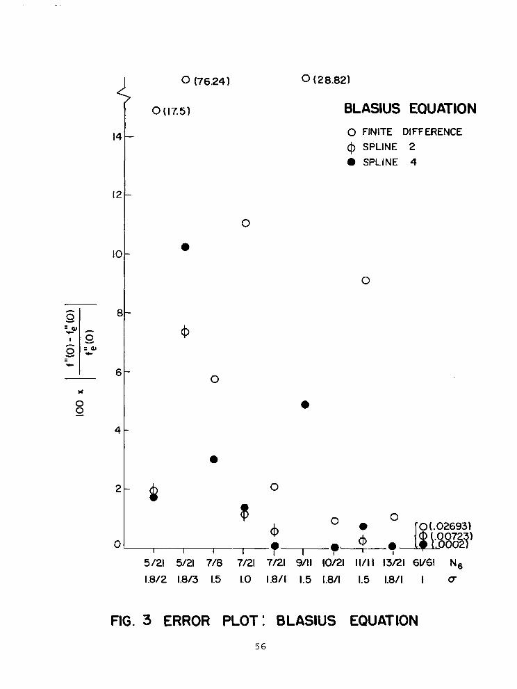
p=O Blas ius so lu t ion :

The s p l i n e 4 s o l u t i o n f o r N=61, h,=0.1 and ~ 1 . 0 i s almost

i den t i ca l w i th t he " exac t " so lu t ion o f f "(o)=O.469600. l4 I f

s p l i n e 2 boundary conditions are used with a s p l i n e 4 i n t e r i o r

po in t formulation,f(o)=O.469608. A s previous ly no ted , th i s va lue

l i e s between the spl ine 2 and s p l i n e 4 r e s u l t s . With 0=1.8/2,

h,=0.5, N = 2 1 and only 5 points in the boundary layer (N6=5),

t h e s p l i n e 2 value of f N ( o ) i s in e r ro r by on ly 2%. For the

l a r g e r h, v a l u e s t h e s p l i n e 2 s o l u t i o n s a r e everA more accura te

than those found wi th sp l ine 4. Similar behavior was observed

with Burgers equat ion in Sect ion V1.A. An e r r o r p l o t i s given

on Figure 3 .

B=1 staqnat ion point f low:

For B=O, the exact solution has u// ' (o)=uiv(o)=O and there-

f o r e t h e i n h e r e n t lower-order accuracy of the f ini te-difference

3 3

c a l c u l a t i o n i s somewhat obscured near the wal l x=O. For the

s t agna t ion po in t so lu t ion where f ” (0) =1.232588, t h e improvement

a s soc ia t ed w i th t he sp l ine fo rmula t ion i s clear ly demonstrated.

Therefore, it would appea r t ha t sp l ine i n t eg ra t ion shou ld be

extremely useful for boundary layer problems.

G. Non-Similar Boundary Layer Analysis

A s a f i n a l tes t of the sp l ine p rocedures the cons tan t

pressure boundary l ayer equa t ions wr i t ten in phys ica l var iab les

(x,y) were considered:

The boundary

uu + vu = Re -1

X Y

u + v = o X Y

cond i t ions a r e

The i n i t i a l c o n d i t i o n s w e r e

U YY

0

given by

The equat ions were i n t e g r a t e d f o r a Reynolds number Re=106 and

a non-uniform mesh of t en po in ts normal to the surface. The

so lu t ion for the normal ized sk in f r ic t ion i s shown on Figure 4.

The value N6 denotes the a c t u a l nunfber o f po in t s w i th in t he

boundary layer. The same c r i t e r i a of Sect ion V1.F was appl ied.

A s t h e boundary layer grows with distance x, N, increases .

With 6 t o 7 po in t s i n t he f i na l boundary l aye r p ro f i l e s , t he

34

spline 4 s o l u t i o n s a r e q u i t e a c c u r a t e .

VII. SUMMARY

It has been demonstrated that h igher-order calculat ion

procedures us ing cubic sp l ine co l loca t ion provide accura te

s o l u t i o n s t o a number of model problems. The s p l i n e methods

termed spl ine 2 and s p l i n e 4 can be used f o r two-point boundary

value problems, as w e l l a s impl ic i t , expl ic i t , two-s tep , AD1

and i t e r a t i v e i n t e g r a t i o n p r o c e d u r e s .

Sp l ine 4 i s fourth-order accurate w i t h a uniform mesh and

th i rd-order wi th a moderate non-uniform mesh. Spl ine 2 i s

second-order accurate for dif fusion terms and fourth-order

( th i rd-order ) for convec t ion wi th a uniform (non-uniform) mesh.

Derivat ive boundary values are obtained direct ly without the

need f o r end d i f f e renc ing . Fo r imp l i c i t l i nea r sys t ems , t he

s p l i n e methods remain unconditionally stable.

The resul ts confirm the higher-order accuracy of the spl ine

methods and lead to t he hope fu l conc lus ion t ha t accu ra t e so lu -

t i o n s f o r more practical flow problems can be obtained with

relat ively coarse non-uniform meshes.

There has been no at tempt to opt imize the temporal inte-

grat ion procedure so a s t o minimize computer times o r i nc rease

temporal accuracy. The f in i t e -d i f f e rence ca l cu la t ions run 20%

t o 25% f a s t e r t h a n t h e s p l i n e i n t e g r a t i o n s . When s p l i n e f i t t i n g

i s used t o e v a l u a t e f i n i t e - d i f f e r e n c e d e r i v a t i v e s , as i n

35

I I I Sect ion VI..C, t h e computer times are comparable. It i s a n t i c i -

pa ted tha t the reduced mesh r equ i r emen t s w i th t hese sp l ine

methods w i l l r e s u l t i n a n e t improvement i n computer storage

and time.

REFERENCES

1. Rubin, S.G. and Graves, R.A., "Cubic Spline Approximation

for Problems in Fluid Mechanics". NASA TR R-436, 1975.

2. Rubin, S.G. and Graves, R.A., "Viscous Flow So lu t ions w i th

a cubic Spline Approximation". Computers and Fluids, 2,

3. Ahlberg, J., Nilson, E. and Walsh, J., The Theory of Splines

and Their Applicat ions. Academic Press, New York, 1967.

4. Papamichael, N. and Whiteman, J., "A Cubic Spline Technique

f o r t h e One-Dimensional Heat conduction Equation". J. I n s t .

5. Peters, N., "Boundary-Layer Calculations by a Hermitian

F in i t e D i f f e rence Method". Four th In t ' l . Conference on

Numerical Methods in Fluid Mechanics, Boulder, Colorado,

1974.

6. Collatz, L., The Numerical Treatment of Differential Equations.

Springer-Verlag, Berlin, 3rd edition, 1960.

7. Orszag, S. and I s r a e l i , M., Numerical Simulation of Viscous

Incompressible Flows. Annual Review of Fluid Mechanics, 5,

1974.

8. HirSh, R., "Higher-Order Accurate Difference Solutions of

Fluid Mechanics Problems by a Compact Differencing Technique".

J . Comp. Phys, 1 9 , 1, Sept. 1 9 7 5 .

36

"

9. Krauss, E., Hirshel, E. H. and Kordulla, W., "Fourth Order

"Mehrste1len"-Integration for Three-Dimensional Turbulent

Boundary Layers". Proc. of AIAA Computational Fluid Dynamics

Conference, Palm Springs, Calif., pp. 92-102, 1973.

10. Fyfe, D. J., "The Use of Cubic Splines in the Solution of

Two-Point Boundary Value Problems". Comput. J., 1 2 ,

pp. 188-192 , 1969 .

11. Brailovskaya, I., " A Difference Scheme for Numerical Solu-

tion of the Two-Dimensional Nonstationary Navier-Stokes

Equations for a Compressible Gas". Soviet Physics-Doklady,

- 10, pp. 1 0 7 - 1 1 0 , 1 9 6 5 .

1 2 . Khosla, P. K. and Rubin, S. G., "A Diagonally Dominant Second-

Order Accurate Implicit Scheme". Computers and Fluids, - 2,

2 , pp. 207-209, 1 9 7 4 .

13 . Roache, P., Computational ~~ " . . Fluid Dynamics. Hermosa Publishers,

Albuquerque, N.M., 1 9 7 2 .

1 4 . Rosenhead, L . , Laminar Boundary Layers, Oxford at the

Clarendon Press, England, 1 9 6 3 .

37

TABLE I SOLUTION OF BURGERS EQUATION v=1/8,# CT = 1.0 31 EQUALLY SPACED POINTS

'x\", 0

- 0.2 - 0.4 - 0.6 - 0.8 - 1.0

- I .2 - 1.4 - 1.6

- 1.8

E 0.

0.5000 0.6999 0.8447 0.9269 0.9693 0.9857 0.9938 0.9973 0.9988 0.9995

SPLINE 2

0.5000 0.6860 0.8290 0.9 I60 0.9620 0.9830 0.9930 0.9970 0.9990 0.9990

____ _"

SPLINE 4

0.5000 0.6900 0.8322 0.9170 0.9609 0.9820 0.991 8 0.9963 0.9983 0.9993

EXACT

0.5000 0.6900 0.8320 0.9 170 0.961 0 0.9820 0.9920 0.9960 0.9980 0.9990

3 8

TABLE 2 SOLUTION OF BURGERS EQUATION v = 1/8, c = 1.2 15 POINTS

0

-0.3859 -0.8494

- I .406C -2.0750 -2.0770

-3.8420 -5.000

. ~~ I __ ~-

SPLINE 2

0.5000

0.82 I4 0.9778

I ,0004 1.0 1.0

I .o I .o

-~~ ~~ ~~~

SPLINE 4

0.5000

0.8297 0.9654 0.995 I 0.9989 0.9999

0.9996 1.0

EXACT

0.5000

0.8240 0.9676

0.9964

0.999 7 1.0

I .o I .o

39

TABLE 3 SOLUTION OF BURGERS EQUATION I/ =I /8, c = 1.8, 15 POINTS

0 -0.0662 -0.1855 -0.4001 -0.7864 - I .4818 -2.9334 -4.9864

SPLINE 2

0.5000 0.5740 0.6986 0.869 5 I .0012

1.0165 I .0267

1.0

SPLINE 4

0.5000 0.5691 0.6858 0.8452 0.9689 I .0083 I .0257

I .o

~ ~. ~___" - -

EXACT

0.5000 0.5659 0.6774 0.832 I 0.9587 0.997 3

1.0

I .o

~~ . ~ ~ . -

40

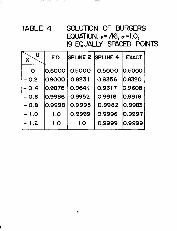
TABLE 4

ED. I-

O

I .o - I .2 I .0 - 1.0

0.9998 - 0.8 0.9986 - 0.6 0.9878 - 0.4 0.9000 - 0.2 0.5000

SOLUTION OF BURGERS

19 EQUALLY SPACED POINTS EQUATION: v=1/16,~=1.0 ,

SPLINE 2

0.5000 0.823 I 0.964 I 0.9952 0.9995

0.9999

1.0

SPLINE 4 1 EXACT

0.5000 0.8356 0.961 7 0.99 I6 0.9982

0.9996

0.9999

0.5000 0.8320 0.9608 0.99 I 8 0.9983

0.9997

0.9999

41

I

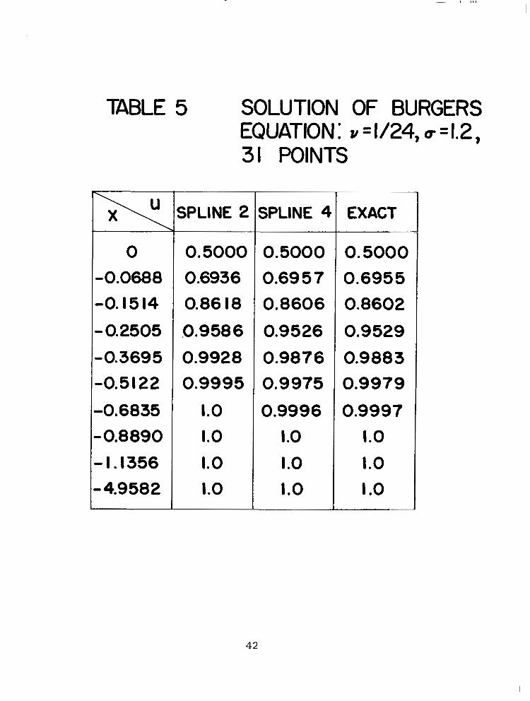
TABLE 5 SOLUTION OF BURGERS

31 POINTS EQUATION: v = 1 / 2 4 , ~ 4 . 2 ,

0 -0.0688 -0. I5 I4 - 0.2505 -0.3695 -0.5122

-0.6835 -0.8890 -1.1356 -4.9582

SPLINE 2

0.5000 0.6936 0.86 I8 .0.9586

0.9928 0.9995

1.0 1.0 1.0 1.0

SPLINE 41

0.5000 0.69 5 7 0.8606

0.9526

0.9876 0.9975 0.9996

I .o I .o I .o

EXACT

0.5000 0.6955 0.8602

0.9529

0.9883 0.9979

0.9997 1.0

I .o I .o

42

TABLE 6 LINEAR BURGERS EQUATION

N FINITE-ELEMENT SPLINE FINITE - DIFFERENCE

10 165.38 37.378(NC) 14.7 25 150.923 100.632 (NC) 50 149.034 132.668 (NC) 100 148.568 144. I37 (NC) 136.022 IO 138.6 (C) -

-

IO - 149. I I5 (C AVG.) - P W

IO ( vuH + 2 U ) = e ”’ AT THE BOUNDARY

165.38 151 552 (NC) 158.969 - 148.486 (C) - ( v u , ) = - e I” AT THE BOUNDARY

- 148.342 (C) - IO 16538 145.442 (NC) 139.296

EXACT SOLUTION U, 8 148.4, v =l/5

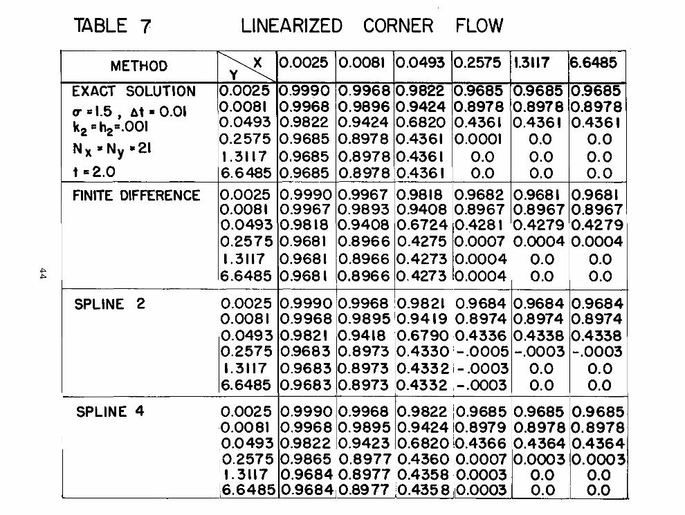
TABLE 7 LINEARIZED CORNER FLOW

P P

METHOD X 0.0025

0.8978 0.8978 0.8978 0.9424 0.9896 0.9968 0.0081 Q 4 . 5 , A t = 0.01 0.9685 0.9685 0.9685 0.9822 0.9968 0.9990 0.0025 EXAGT SOLUTION

6.6485 1.3117 0.2575 0.0493 0.0081

k, = h.p.001 0.0493 0.9822 0.9424 0.436 I 0.436 I 0.4361 0.6820 0.2575

0.0 0.0 0.0 0.4361 0.8978 0.9685 6.6485 t p2.0 0.0 0.0 0.0 0.4361 0.8978 0.9685 I .3117 Nx 'Ny ~ 2 1 0.0 0.0 0.0001 0.4361 0.8978 0.9685

FINITE DIFFERENCE 0.008 I 0.0025

0.2575 0.0493

6.6485 1.3117

SPLINE 2 0.0025 0.008 I 0.0493 0.2575 1.3117 6.6485

SPLINE 4 0.0025 0.0081 0.0493 r0.2575

0.9990

~0.0004 0.4273 0.8966 0.968 I '0.0004 0.4273 0.8966 0.968 I' 0.0007 0.4275 0.8966 0.9681 i0.428 I 0.6724 0.9408 0.98 18 ,0.8967 0.9408 0.9893 0.9967 0.9682 0.9818 0.9967

4- 0.9990 0.9968 0.9821 '10.9684 0.9968 0.9895 0.94 19 /0.8974 0.982 I 0.9418 0.6790 10.4336 0.9683

0.4332 t - .0003 0.8973 0.9683 0.4330 ~ -.0005 0.8973

0.9683 10.4332 ,-.0003 0.8973

0.9990

0.6820 10.4366 '0.9423 0.9822 0.9424 !0.8979 0.9895 0.9968 i0.9822 '0.9685 10.9968

0.4360 ,i0.0007 0.4358 ;0.0003 i0.435 8 j0.0003

0.968 I

0.0004 0.0004 0.4279 0.4279 0.8967 0.8967 0.968 I

0.0 0.0 0 .o 0.0

0.9684 0.9684 0.8974 0.8974 0.4338 0.4338 -.0003 -.0003 0.0 0.0 0.0 0.0

0.9685 ~ 0.9685 0.8978 10.897e 0.4364 10.4364 0.0003 !O.OOO? 0.0 ' 0.0

~ ~~~~~~

, 0.0 1 0.0

TABLE 8

EQUATION SOLUTION OF THE

METHOD EXACT SOLUTION FINITE DIFFERENCE SPLINE 2 SPLINE 4X, SPLINE 2 Y SPLINE 4 EXACT SOLUTION SPLINE 4 SPLINE 4 X , SPLINE 2 Y FINITE DIFFERENCE

EXACT SOLUTION FINITE DIFFERENCE SPLINE 2 SPLINE 4X, SPLINE 2Y SPLINE 4 EXACT SOLUTION FINITE DIFFERENCE SPLINE 2 SPLINE . . 4X, SPLINE 2 Y EXACT SOLUTION FINITE DIFFERENCE SPLINE 4X, SPLINE 2 Y SPLINE 4 EXACT SOLUTION FINITE DIFFERENCE SPLINE 2 SPLINE 4X, SPLINE 2 Y SPLINE 4

.. ~ ~

.. ". ~~ ~ ~

~~~ "~ "_ .. . . - -

~~ . . .. .-

_ _ - ~ - "" ~ ~ ~ "- ~ ~~~

~. ~ "- ~ - . ~ " ~ ~~

. ~ ". ~~~

-U p , O ] 3.142 3.123 3.164 3. I54 3. I42

3. I42 3.162 3.193 2.828*

3.142 3.189 3 . 175 3 . I62 3.137

3.142 3 193 3.177 3.164 3.142 3.220 3 185 3 .I30 3. I416 3.1694 3. I676 3.155l 3.1404

- - " . -

~~~~ ~~

-

. . ."

-

LAPLACE

"

u (-5,Q 0.7304 0.7322 0.7286 0.7295 0.7304 0.5335 0.5329 0.5277 0.540 I

0.969T 0.9686 0.9687 0.9689 0.969 I

0.939 I 0.938 I 0.9384 0.9387 0.7304 0.7233 0.7263 0.7313 0.9691 3.9688 0.9688 3.9689 D.9691

~- ~.

-~ ~~ ~~ ~ ~~

: 1 = /k, 1.0 0.1

I .o 0. I

I .7

I .7

I .7

3. I

0. I

0. I

0. I

h2 0. I

3.2

3.01

3.02

0. I

0.01

'MAX 1.0

2.0

2.86

2.73

28.66

1.063

* EVALUATED BY 3-POlNT END-DIFFERENCE FORMULA

45

!

TABLE 9

METHOD

EXACT SOLUTION A 8 = T/K) h, = 0.05 cr = 1.7 rMAX= 15.3285

~~ ~

FINITE DIFFERENCE

~

SPLINE 2

' SPLINE 4 I

I

I

POTENTIAL CYLINDER

1;0500 I .279 5 I .9428 3.8596 9.3991

I. 0500 1.2795 1.9428 3.8 596 9.3991

1.0500 1.2795 1.9428 3.8596 9.399 I

1.0500 I .27 95 1.9428 3.8596 9.399 I L

FLOW

0

2.0024 2.061 I 2.4 575 4. I I87 9.5055

I ,8626 I .9365 2.3597 4.0573 9.461 8

1.9249 I .9821 2.3726 4.0285 9.4254

2.0089 2.0677 2.4 639 4.1 I85 9.4760

OVER

T /IO

1.9044 1.9602 2.3372 3.9171 9.0403

1.7714 1.8417 2.2442 3.8587 0.9987

1.8307 1.8851 2.2 565 3.83 I 4 8.9641

I .9l06 I .9665 2* 343 Z 3.9 I69 9.0122

-

A

2 d I 0

1.6200 I .6674 I .988 I 3.332 I 7.690 I

I .5069 I .56 67 I .go9 I 3.2824 7.6547

I .5 573 1.6035 1.9195 3.259 I 7.6253

1.6253 1.6728 1.9934 3.33 19 7.6663

CIRCULAR

37-r /IO

I. I770 1.21 15 1.4445 2.4209 5.5872

10948 I . 1383 1.3871 2.3848 5.5615

1.1314 I. 1650 I. 3946 2.367 9 5.5401

I. I808 I. 2154 I . 4483 2.4208 5.5699

"~

4 d o 0.6188 0.6369 0.7594 I .2727 2.9374

0.5757 0.59 8 5 0.7293 I .2538 2.9239

0.5948 0.6 I 25 0.7 33 2 I .2449 2.9 126

0.6208 0.6390 0.761 4 I .2727 2.9283

TABLE IO POTENTIAL FLOW OVER A CIRCULAR CYLINDER

I

METHOD

EXACT SOLUTION Il.0500 ! A 8 = n /20 : L279 5 .I h2 00.05 1.9428 i Q 01.7 I 3.8596 1

MAX = 15.3285 #'9.399 I FIN IT€ DIFFERENCE

P ' 4 ,

I SPLINE 2

I

1.0500 1.2795 1.9 428 3.8596 9.399 I

1.0500 1.27 9 5 1.9428 3.8596 9.399 I

I .O 500 I .27 95 I .9 428 3.8596 9.399 I

0 ! n/10 2lr/10 1 3r/IO 1 4 d 0

2.0024 I1.9044 11.6200 ' 1.1770 0.6188 ~ I

I i

2.061 I 2.4575 4. I187 9.5055

I ,9246 I .9830 2.3816 4.0551 9.4506

I .94l3 1.9986 2.3898 4.0474 9.4399

2.0094 2.0682 2.464 3 4. I188 9.4762

i.

"

1.9602 ~ 1.6674 2.3372 j 1.9881 3.9 I7 I ,3.332 I 9.0403 i 16901

1.2115 1.4445

2.4209 5.58 7 2

0.6369 0.7594

I I .2727 ~ 2,9374 -

1.8304 11.5571 * ' 1.1313 0.5949 1.8859 1.6043 1.1657 0.6130 2.2650 1.9268 1.4000 ,0.7361

3.2807 2.3836 1.2532 7.6457 I5.5549 I2.9204

1 "

1.8463 1 1.5706 11.1412 I1 1.9008 11.6169

2.2728 I .9334 3.8494 8.9778

1.9111 I .9670 2.3437 3.9172 9.0 124

3.2745 7.6370

I .6257 I .6732 I .9938 3.3323 7.6664

I . 1749 I .4048 2.379 I 5.5486

I .I813 I .2158 I. 4487 2.421 I 5.5700

-c 1 0.600 I 0.6178 0.7387 I 2509 2.9171

0.62 12 0.6394 0.761 8 1'2730 2.9284

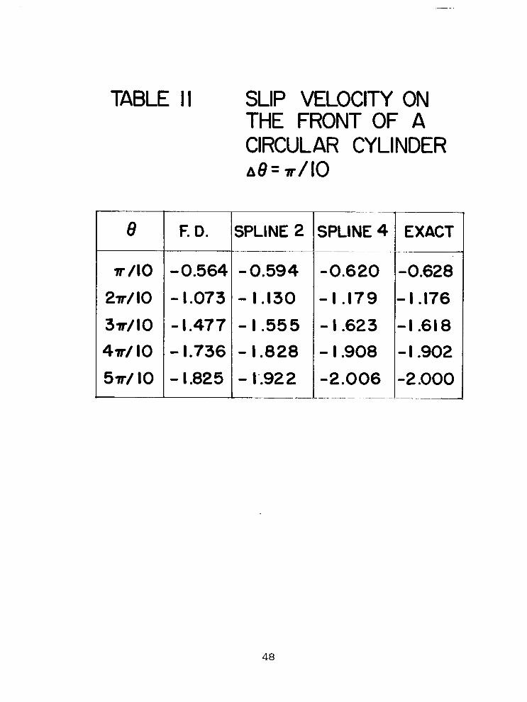
TABLE II SLIP VELOCITY ON THE FRONT OF A CIRCULAR CYLINDER ~ 8 = 4 0

8

7T /IO

27r/ IO

3d10 47r/ IO

57r/ IO

F. 0. SPLINE 2

-0.564 - I .073 - I .477 - 1.736

- I .825

-0.594

- I .I30

- 1.555 - 1.828

- 1‘.922 -___ ”

SPLINE 4

-0.620

- I .I79

- I .623 - I .908

-2.006

____ ~ . .

-0.628

- I .I76

-I .618 -I .902

-2 .ooo -

48

TABLE I2 BLASIUS PROFILE: u 4.0, h,=0.1, N=61

f f ' X EXACT SPLINE 4 SPLINE 2 E 0. SPLINE 4: EXACT SPLINE 2 F: 0.

~ _ _ ~

1

0. I

0.371963 0.371964 0.371934 0.372076 0.149675 0.149675 0.149673 0.149697 0.8 0.280575 0.280576 0.280563 0.280651 0.084386 0.084386 0.084387 0.084399 0.6 0. I87605 0.187605 0.187604 0.087648 0.0375490.037549 0.03755 I 0.037555 0.4 0.093905 0.093905 0.093908 0.093923 0.00939 I 'i0.00939 I 0.009392 0.009392 0.2 0.046959 0.046959 0.046967,0.046962 0.0023481.0.002348 0.002348.0.002348

I .O 0.233026 0.232982 0.2329900.232990 0.460788 0.460583

I .o 1.0 1.0 I .o 4.783217 4.783220 4.783110 4.783607 610 0.9W770 0.997771 0.997790 0.997824 2.783885 2.783890 2.783770 2.784256 4.0 0.816694 0.816695 0.816600 0.817023 0.886796 0,886798 0.8869380.886707 2.0 0.661473 0.661474 0.661379 0.661735 0.51503 I 0.515032 0.514990 0.5151 I I I .5 0.460632 0.460633

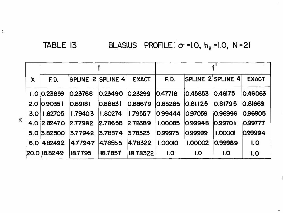
TABLE 13 BLASIUS PROFILE c =LO, h, =LO, N =21

X E 0.

1 .O 0.23859

2.0

3.82500 5 .O 2.82470 4.0 I ,82705 3.0 0.9035 I

18.8249 20.0

4.8249 2 6.0

f SPLINE 2 SPLINE 4

3.23768 0.23490

3.8918 I

3.78874 3.77942

2.78658 2.77982 I ,80274 I ,7940 3 0.8883 I

18.7857 18.7795

4.7855 5 4.77947

EXACT

0.23299

0.88679

I ,7955 7 2.78389

3.78323

4.78322

18.78322

F. 0.

0.47718

0.85265 0.99444 I ,00085

0.99975

I .00010 1.0

f ' SPLINE 2 EXACT SPLINE 4

0.45853 0.46175

0.81669 0.8179 5 0.81 I25 0.46063

I. 0 0.99989 I ,00002 0.99994 1 . o o o O 1 099999

099777 09970 I 3.99948 0.96905 0.96996 097059

I .o 1.0 1.0

TABLE 14 BLASIUS PROFILE:C=I.~/, , h,=0.5, N =21

X

0.5

I .4 2.4

3.4 4.4

5.4

19.4

f E 0. 2iSPLINE 4 SPLINE

0.05910

18.18380 18.1698 18.2155

4.18386 4.16985 4.21548

3.18422 3.16972 3.21568

2.19064 2.17478 2.21456

1.24067 I .2253 I I .24551 0.45722 0.4505 I 0.45557

0.05888 0.05835

EXACT

0.05864

0.45072 I .23153

2.18747

3.18338

4.18322

18. I8322

T f '

TABLE

XMAX

6.0 20.0

5.6665 I I .3=0 6.4344 13.365

16.063

19.400

37.020

53.936 ~

f " (0)

15

h2

0. I I .o

0.05 0. I 0.2 0.0 I

3.05

0.5

0.5

0.5

Q

I .o 1.0 1.5 1.5 I .5

1% 1.

f"(0) FOR

FIN IT€ DIFFERENCE 0.4697265 0.52804 I 0.516646 0.6049558 0.498214 0.474643

1.81 0.473974 1.

1.81 I 0.4797 15

I.8I2. 10.551803

l.8/3. 10.827648

BLASIUS EQUATION

SPLINE 2 I SPLINE 4

0.469634 0.469601 0.475357

0.466048 0.4707 I8 0.476359

-0.493598 - - 0.455623

0.469188

- - 0.469438

0.466839 0.469509

0.460823 0.477930

0.506798 0.523256

~- .. -

-

-

~~ ~-

10.469600 (ROSENHEAD ) (16)

~~~

Ne/N

31/61 71 21 II/ I I

9/1 I 7/8

13/21

10/2 I

7/21

5/21

5/21

52

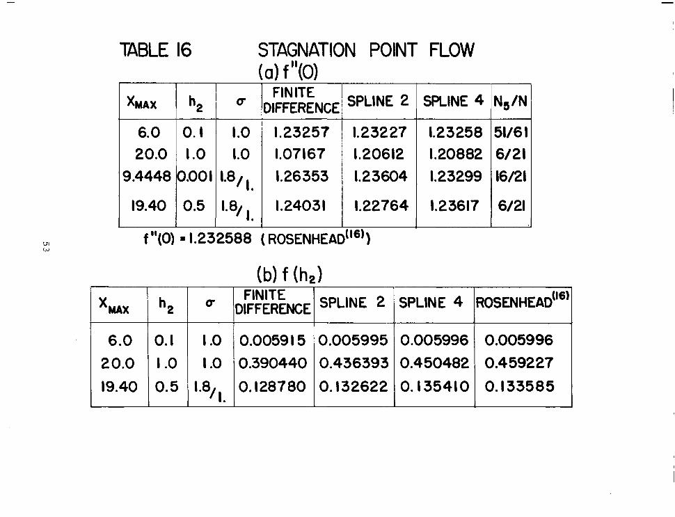
TABLE 16

6.0

0.00 I 9.4448 1.0 20.0 0.1

19.40 0.5

STAGNATION POINT FLOW

" FINITE IIFFERENCE

1.23257 1.07167 1.26353

1,24031

1.23227

16/21 1.23299 1.23604 6/21 1.20882 1.20612 51/61 1.23258

1 1.22764 1.23617 6/21

f "(0) = 1.232588 (ROSENHEAI

*MAX I h2

6.0

0.5 19.40

I .o 20.0 0.1 I .O 0.00591 5

I .O 0.390440 0. I28780 1.

SPLINE 2 ROSENHEAD SPLINE 4 ( 7

0.005995

0. I33585 0. I35410 0.132622 0.459227 0.450482 0.436393 0.005996 0.005996

1 . 4 -

1.2 -

I .o-

0.8 r

0

0

"

0.4 1-

BURGERS EQUATION

0 FINITE DIFFERENCE @ SPLINE 2 0 SPLINE 4

0

0

0

0.21- 0 I

1 , Q 0 Q 0 8 0 L o - e 0- 0 0 0 0 0.2 0.4 0.6 0.8 1.0 1.2 I .4 1.6

1x1

FIG. I NON-LINEAR BURGERS EQUATION: ~81/8, Q 8 I

2.4

2 .o

0.e

0.4

0

LAPLACE EQUATION 0

' 0 FINITE DIFFERENCE (DERIVATIVE WITH SPLINE) 4 SPLINE 2

0 SPLINE 4

0

0

9 8

8 0

0 0

I 1 1 P- O .01/17 .02 A.7 .01/1.7/2 . I /LO . I 11.7

h,

FIG. 2 LAPLACE EQUATION

5 5

14

12

IC

E

6

4

2

0

0 (76.24) 0 (28.82)

BLASIUS EQUATION 0 FINITE DIFFERENCE @ SPLINE 2 0 SPLINE 4

0

0

0

0

0

0

b 0

5 /21 5/21 7/8 7/21 7/21 911 I 10121 I1/1 I 13/21 6V61 N,

1.812 1.86 1.5 1.0 1.811 1.5 1.811 1.5 1.811 I U

FIG. 3 ERROR PLOT: BLASIUS EQUATION

5 6

. 4 0

c

0 x‘ CI

=I r

.36

.3 2

.2 0

4”

- ””“ c -~

/

SIMILARITY SOLUTION-.4696

FINITE DIFFERENCE ” - SPLINE 4

u =1.5 h, = .OOl

N = I O R, = lo5

2 4 I I I I I I I I I

0 0.2 0.4 0.6 0.8 I. 0 I .2 I .4 1.6 X

4 5 6 7 N6

FIG.4 CONSTANT PRESSURE BOUNDARY LAYER SOLUTION - PHYSICAL VARIABLES