Chapter 1

Higher Order SlidingModes as a NaturalPhenomenon in ControlTheory

Introduction

Sliding modes are used in order to keep a dynamic system to given con-straints with utmost precision. They are also insensitive to external andinternal disturbances. These features are provided due to a theoreticallyinfinite frequency of control switching. At the same time, any presence ofreal actuators and measuring devices may cause considerable change in thereal system behavior. There are also many arguments for the use of con-tinuous controllers as approximations for discontinuous ones. Both reasonslead to the replacement of regular sliding modes in real systems by somespecial ones. Consider the phenomenon more explicitly.

A. Presence of fast actuators

Let the constraint be given by the equality of some constraint functionσ to zero and the sliding mode σ ≡ 0 be provided by a relay control.Taking into account an actuator conducting a control signal to the processcontrolled, we achieve a more complicated dynamics. In this case a relaycontrol enters the actuator and continuous output variables of the actuator

Plant

Relay Controller

Actuator

¾

6

-

Figure 1.1: Control system with actuator

are transmitted to the plant input ( Fig. 1.1). As a result discontinuousswitching is hidden now in the higher derivatives of the constraint function[36, 37, 15, 16, 17, 18, 19, 20].

B. Artificial actuator-like dynamics

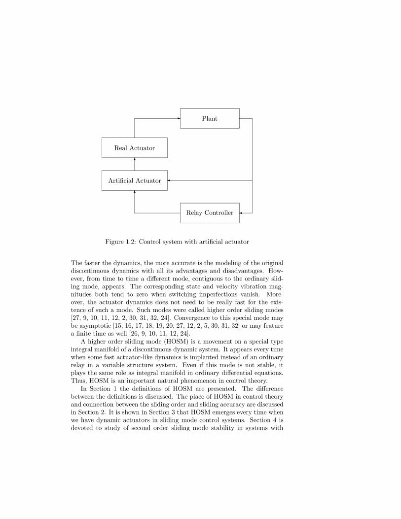
One of the main known drawbacks of regular sliding modes is the so-calledchattering effect which is exhibited by high frequency vibration of the plant.This vibration features some definite vibration magnitude of the plant itself(in the state space) and of the plant velocity. While the first magnitudeis infinitesimally small when switching imperfections (like switching delay)tend to zero, the second is approximately constant and eventually evenlarge. Therefore the high frequency vibration energy is also finite or evenlarge which may cause a system disaster. To avoid chattering several ap-proaches have been proposed. The main idea is to change the dynamics ina small vicinity of the discontinuity surface in order to avoid real discon-tinuity and at the same time to preserve the main properties of the wholesystem. A transition to the new dynamics defined near the switching sur-face has to be sufficiently smooth. The idea is realized by insertion of someartificial actuator (Fig. 1.2). This actuator may be a functional [33] ormay have its own dynamics [8, 7]. We are interested here in the latter case.

The actuator installed (artificial or real) has mainly some fast dynamics.

Plant

Relay Controller

Artificial Actuator

Real Actuator

¾

¾

6

6

-

Figure 1.2: Control system with artificial actuator

The faster the dynamics, the more accurate is the modeling of the originaldiscontinuous dynamics with all its advantages and disadvantages. How-ever, from time to time a different mode, contiguous to the ordinary slid-ing mode, appears. The corresponding state and velocity vibration mag-nitudes both tend to zero when switching imperfections vanish. More-over, the actuator dynamics does not need to be really fast for the exis-tence of such a mode. Such modes were called higher order sliding modes[27, 9, 10, 11, 12, 2, 30, 31, 32, 24]. Convergence to this special mode maybe asymptotic [15, 16, 17, 18, 19, 20, 27, 12, 2, 5, 30, 31, 32] or may featurea finite time as well [26, 9, 10, 11, 12, 24].A higher order sliding mode (HOSM) is a movement on a special type

integral manifold of a discontinuous dynamic system. It appears every timewhen some fast actuator-like dynamics is implanted instead of an ordinaryrelay in a variable structure system. Even if this mode is not stable, itplays the same role as integral manifold in ordinary differential equations.Thus, HOSM is an important natural phenomenon in control theory.In Section 1 the definitions of HOSM are presented. The difference

between the definitions is discussed. The place of HOSM in control theoryand connection between the sliding order and sliding accuracy are discussedin Section 2. It is shown in Section 3 that HOSM emerges every time whenwe have dynamic actuators in sliding mode control systems. Section 4 isdevoted to study of second order sliding mode stability in systems with

actuators. Various examples of second order sliding modes are presentedin Section 5. Section 6 deals with examples of higher order sliding modes,an example of third order sliding algorithm with finite convergence time ispresented.

1.1 Definitions of higher order sliding modes

Regular sliding mode features few special properties. It is reached in finitetime which means that the shift operator along the phase trajectory exists,but is not invertible in time at any sliding point. Other important featuresare that the manifold of sliding motions has a nonzero codimension andthat any sliding motion is performed on a system discontinuity surface andmay be understood only as a limit of motions when switching imperfectionsvanish and switching frequency tends to infinity. Any generalization of thesliding mode notion has to inherit some of these properties. A definitiondeveloped in [4] deals with the first property and allows, thus, extensionof the definition to dynamic systems of even completely different nature.The definitions developed below utilize the other properties mentioned. Inmany cases both definition systems are satisfied (not only in the case of theregular sliding mode).Let us remind first what are Filippov’s solutions [13, 14] of a discontin-

uous differential equationx = v(x),

where x ∈ Rn, v is a locally bounded measurable (Lebesgue) vector func-tion. In this case, the equation is replaced by an equivalent differentialinclusion

x ∈ V (x).

In the particular case when the vector-field v is continuous almost every-where, the set-valued function V (x) is the convex closure of the set of allpossible limits of v(y) as y → x, while {y} are continuity points of v. Anysolution of the equation is defined as an absolutely continuous function x(t),satisfying the differential inclusion almost everywhere.In the following Definitions we follow the works by Levantovsky [26],

Emelyanov et. al. [9, 10, 12], Levant [24].

1.1.1 Sliding modes on manifolds

Definition 1 Let L be a smooth manifold. Set L itself is called the firstorder sliding set with respect to L. The second order sliding set is definedas the set of points x ∈ L, where V (x) lies entirely in tangential space TLto manifold L at point x.

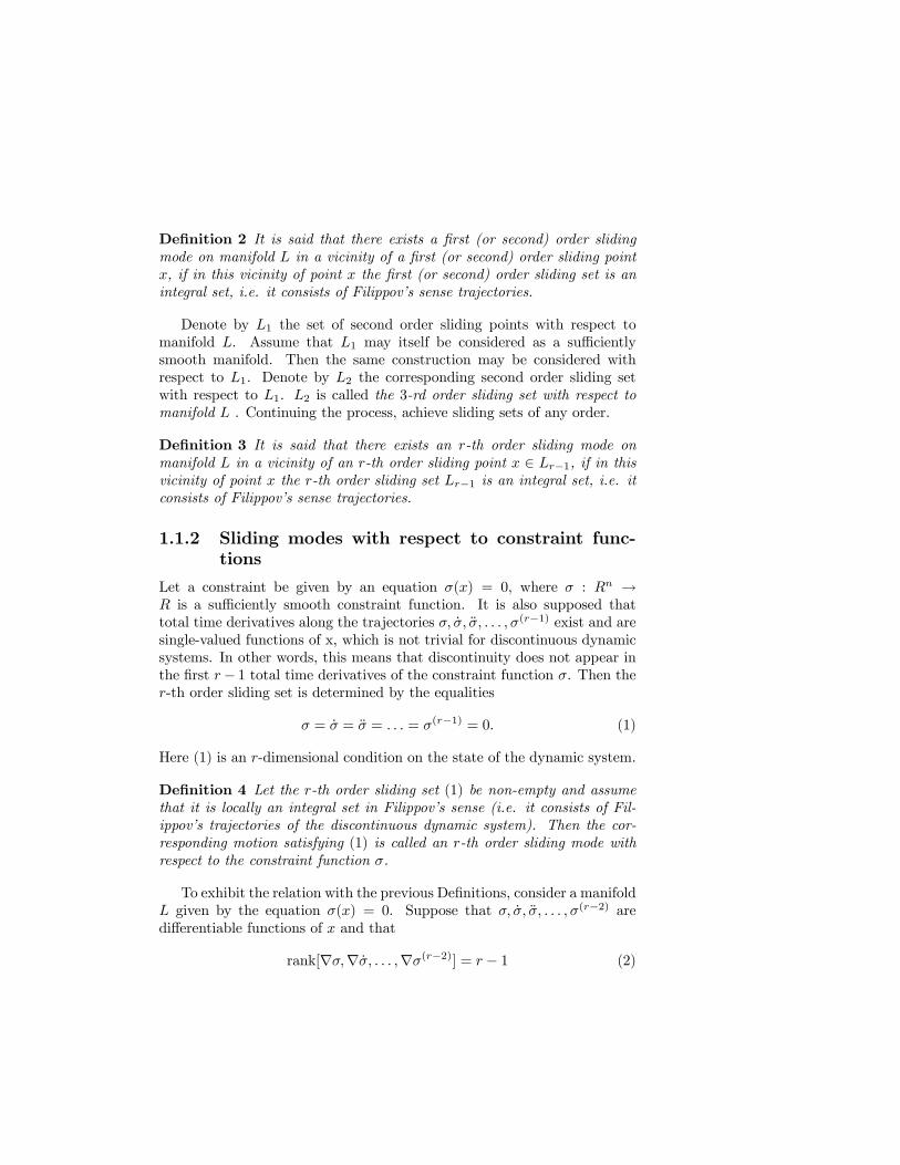
Definition 2 It is said that there exists a first (or second) order slidingmode on manifold L in a vicinity of a first (or second) order sliding pointx, if in this vicinity of point x the first (or second) order sliding set is anintegral set, i.e. it consists of Filippov’s sense trajectories.

Denote by L1 the set of second order sliding points with respect tomanifold L. Assume that L1 may itself be considered as a sufficientlysmooth manifold. Then the same construction may be considered withrespect to L1. Denote by L2 the corresponding second order sliding setwith respect to L1. L2 is called the 3-rd order sliding set with respect tomanifold L . Continuing the process, achieve sliding sets of any order.

Definition 3 It is said that there exists an r-th order sliding mode onmanifold L in a vicinity of an r-th order sliding point x ∈ Lr−1, if in thisvicinity of point x the r-th order sliding set Lr−1 is an integral set, i.e. itconsists of Filippov’s sense trajectories.

1.1.2 Sliding modes with respect to constraint func-tions

Let a constraint be given by an equation σ(x) = 0, where σ : Rn →R is a sufficiently smooth constraint function. It is also supposed thattotal time derivatives along the trajectories σ, σ, σ, . . . , σ(r−1) exist and aresingle-valued functions of x, which is not trivial for discontinuous dynamicsystems. In other words, this means that discontinuity does not appear inthe first r− 1 total time derivatives of the constraint function σ. Then ther-th order sliding set is determined by the equalities

σ = σ = σ = . . . = σ(r−1) = 0. (1)

Here (1) is an r-dimensional condition on the state of the dynamic system.

Definition 4 Let the r-th order sliding set (1) be non-empty and assumethat it is locally an integral set in Filippov’s sense (i.e. it consists of Fil-ippov’s trajectories of the discontinuous dynamic system). Then the cor-responding motion satisfying (1) is called an r-th order sliding mode withrespect to the constraint function σ.

To exhibit the relation with the previous Definitions, consider a manifoldL given by the equation σ(x) = 0. Suppose that σ, σ, σ, . . . , σ(r−2) aredifferentiable functions of x and that

rank[∇σ,∇σ, . . . ,∇σ(r−2)] = r − 1 (2)

holds locally. Then Lr−1 is determined by (1) and all Li, i = 1, . . . , r − 2are smooth manifolds. If in its turn Lr−1 is required to be a differentiablemanifold, then the latter condition is extended to

rank[∇σ,∇σ, . . . ,∇σ(r−1)] = r (3)

Equality (3) together with the requirement for the corresponding deriv-atives of σ to be differentiable functions of x will be referred to as the slidingregularity condition, whereas condition (2) will be called the weak slidingregularity condition.With the weak regularity condition satisfied and L given by the equation

σ = 0 Definition 4 is equivalent to Definition 3. If the regularity condition(3) holds, then new local coordinates may be taken. In these coordinatesthe system will take the form

y1 = σ, y1 = y2; . . . ; yr−1 = yr;

σ(r) = yr = Φ(y, ξ);

ξ = Ψ(y, ξ), ξ ∈ Rn−r.

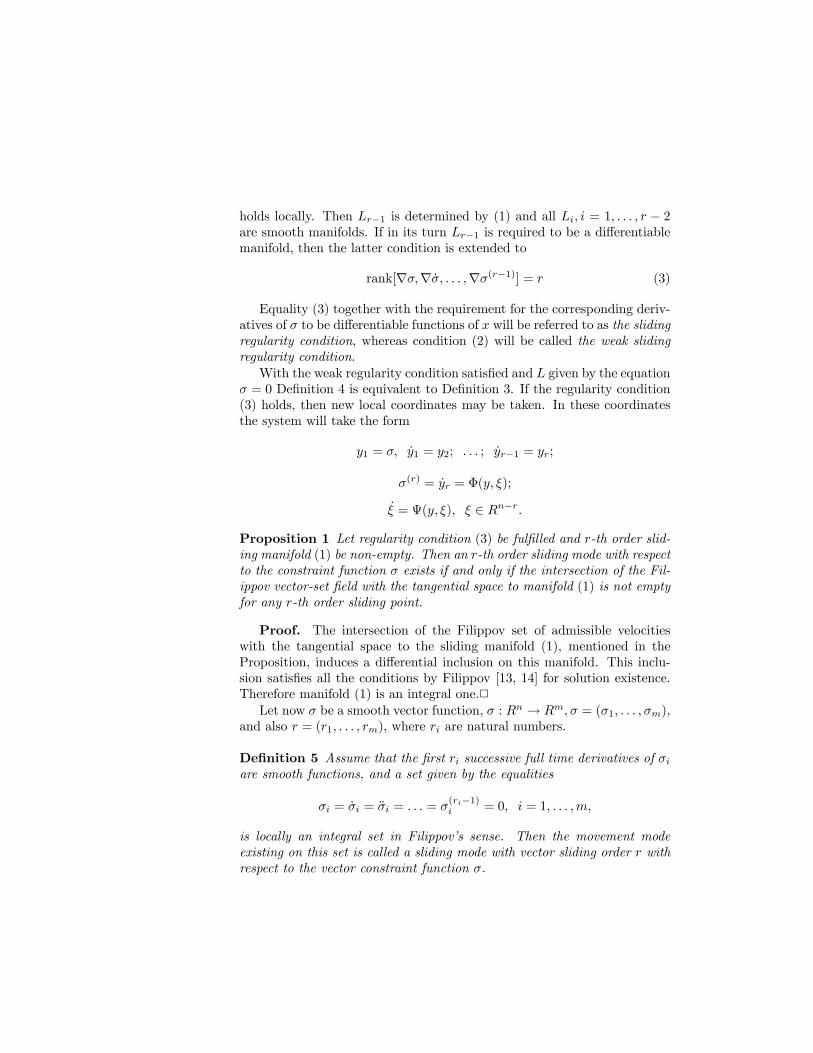
Proposition 1 Let regularity condition (3) be fulfilled and r-th order slid-ing manifold (1) be non-empty. Then an r-th order sliding mode with respectto the constraint function σ exists if and only if the intersection of the Fil-ippov vector-set field with the tangential space to manifold (1) is not emptyfor any r-th order sliding point.

Proof. The intersection of the Filippov set of admissible velocitieswith the tangential space to the sliding manifold (1), mentioned in theProposition, induces a differential inclusion on this manifold. This inclu-sion satisfies all the conditions by Filippov [13, 14] for solution existence.Therefore manifold (1) is an integral one.2Let now σ be a smooth vector function, σ : Rn → Rm, σ = (σ1, . . . , σm),

and also r = (r1, . . . , rm), where ri are natural numbers.

Definition 5 Assume that the first ri successive full time derivatives of σiare smooth functions, and a set given by the equalities

σi = σi = σi = . . . = σ(ri−1)i = 0, i = 1, . . . ,m,

is locally an integral set in Filippov’s sense. Then the movement modeexisting on this set is called a sliding mode with vector sliding order r withrespect to the vector constraint function σ.

The corresponding sliding regularity condition has the form

rank{∇σi, . . . ,∇σ(ri−1)i |i = 1, . . . ,m} = r1 + . . .+ rm.

Definition 5 corresponds to Definition 3 in the case when r1 = . . . = rmand the appropriate weak regularity condition holds.A sliding mode is called stable if the corresponding integral sliding set

is stable.

Remarks.

1. These definitions also include trivial cases of an integral manifold in asmooth system. To exclude them we may, for example, call a sliding mode”not trivial” if the corresponding Filippov set of admissible velocities V (x)consists of more than one vector.2. The above definitions are easily extended to include non-autonomous

differential equations by introduction of the fictitious equation t = 1

1.2 Higher order sliding modes in control sys-tems

All the previous considerations are translated literally to the case of aprocess controlled

x = f(t, x, u), σ = σ(t, x) ∈ R, u = U(t, x) ∈ R,

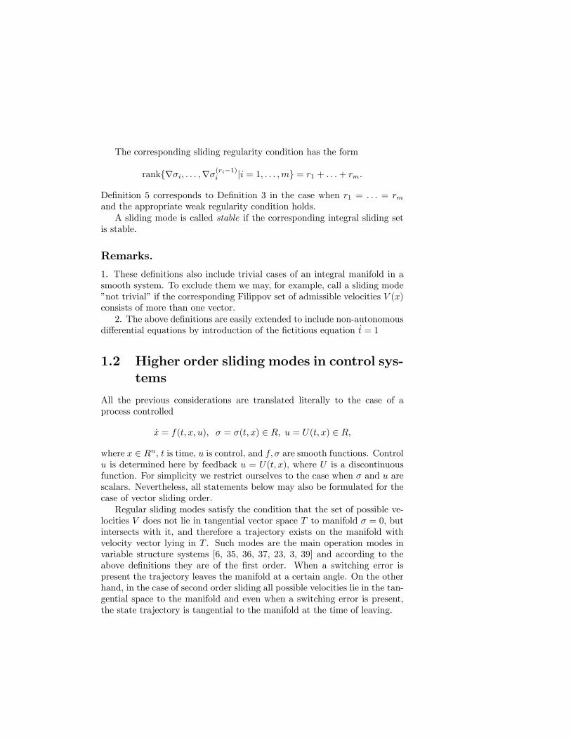
where x ∈ Rn, t is time, u is control, and f, σ are smooth functions. Controlu is determined here by feedback u = U(t, x), where U is a discontinuousfunction. For simplicity we restrict ourselves to the case when σ and u arescalars. Nevertheless, all statements below may also be formulated for thecase of vector sliding order.Regular sliding modes satisfy the condition that the set of possible ve-

locities V does not lie in tangential vector space T to manifold σ = 0, butintersects with it, and therefore a trajectory exists on the manifold withvelocity vector lying in T . Such modes are the main operation modes invariable structure systems [6, 35, 36, 37, 23, 3, 39] and according to theabove definitions they are of the first order. When a switching error ispresent the trajectory leaves the manifold at a certain angle. On the otherhand, in the case of second order sliding all possible velocities lie in the tan-gential space to the manifold and even when a switching error is present,the state trajectory is tangential to the manifold at the time of leaving.

To see connections with some well-known results of control theory, con-sider at first the case when

x = a(x) + b(x)u, σ = σ(x) ∈ R, u ∈ R,

where a, b, σ are smooth vector functions. Let the system have a relativedegree r with respect to the output variable σ (Isidory [22]). This meansthat Lie derivatives Lbσ,LbLaσ, . . . , LbL

r−2a σ equal zero identically in a

vicinity of a given point and LbLr−1a σ is not zero at the point. The equality

of the relative degree to r means, in a simplified way, that u first appearsexplicitly only in the r-th full time derivative of σ. It is known that in thiscase σ(i) = Liaσ for i = 1, . . . , r − 1, regularity condition (3) is satisfiedautomatically and also ∂uσ

(r) = LbLr−1a σ 6= 0. There is a direct analogy

between the relative degree notion and the sliding regularity condition.Loosely speaking, it may be said that the sliding regularity condition (3)means that the ”relative degree with respect to discontinuity” is not lessthan r. Similarly, the r-th order sliding mode notion is analogous to thezero-dynamics notion.The relative degree notion was originally introduced for the autonomous

case only. Nevertheless, we will apply this notion to the non-autonomouscase as well. As was already done above, we introduce for this purpose afictitious variable xn+1 = t, xn+1 = 1. It has to be mentioned that someresults by Isidory will not be correct in this case, but the facts listed in theprevious paragraph will still be true.Consider a dynamic system of the form

x = a(t, x) + b(t, x)u, σ = σ(t, x), u = U(t, x) ∈ R.

Theorem 1 Let the system have relative degree r with respect to the outputfunction σ at some r-th order sliding point (t0, x0). Let, also, the discontin-uous function U take on values from sets [K,∞) and (−∞,−K] on somesets of non-zero measure in any vicinity of any r-th order sliding pointnear point (t0, x0). Then this provides, with sufficiently large K, for theexistence of r-th order sliding mode in some vicinity of point (t0, x0).

Proof. This Theorem is an immediate consequence of Proposition 1,nevertheless, we will detail the proof. Consider some new local coordinatesy = (y1, . . . , yn), where y1 = σ, y2 = σ, . . . , yr = σ(r−1). In these coordi-nates manifold Lr−1 is given by the equalities y1 = y2 = . . . = yr = 0 andthe dynamics of the system is as follows:

y1 = y2, . . . , yr−1 = yr,yr = h(t, y) + g(t, y)u, g(t, y) 6= 0,ξ = Ψ1(t, y) +Ψ2(t, y)u, ξ = (yr+1, . . . , yn)

(4)

Denote Ueq = −h(t, y)/g(t, y). It is obvious that with initial conditionsbeing on the r-th order sliding manifold Lr−1 control u = Ueq(t, y) providesfor keeping the system within manifold Lr−1. It is also easy to see that thesubstitution of all possible values from [−K,K] for u gives us a subset ofvalues from Filippov’s set of the possible velocities. Let |Ueq| be less thanK0, then with K > K0 the substitution u = Ueq determines a Filippov’ssolution of the discontinuous system which proves the Theorem. 2The trivial control algorithm u = −K signσ satisfies Theorem 1. Usu-

ally, however, such a mode will not be stable.It follows from the proof above that the movement in the r-th order

sliding mode is described by the equivalent control method (Utkin [35]),on the other hand this dynamics coincides with the zero-dynamics [22] forcorresponding systems.There are some recent papers devoted to the higher order sliding mode

technique. The sliding mode order notion, which appeared in 1990 [2, 5],seems to be understood in a very close sense (the authors had no possibilityto acquaint themselves with the work by Chang [2]). The same idea isdeveloped in a very general way from the differential-algebraic point ofview in the papers by Sira-Ramirez [30, 31, 32]. In his papers sliding modesare not distinguished from the algorithms generating them. Consider thisapproach.Let the following equality be fulfilled identically as a consequence of the

dynamic system equations [32]:

P (σ(r), . . . , σ, σ, x, u(k), . . . , u, u) = 0. (5)

Equation (5) is supposed to be solvable with respect to σ(r) and u(k). Func-tion σ may itself depend on u. The r-th order sliding mode is considered asa steady state σ ≡ 0 to be achieved by a controller satisfying (5). In orderto achieve for σ some stable dynamics

Σ = σ(r−1) + a1σ(r−2) + . . .+ ar−1σ = 0

the discontinuous dynamics

Σ = −signΣ (6)

is provided. For this purpose the corresponding value of σ(r) is evaluatedfrom (6) and substituted into (5). The obtained equation is solved for u(k).Thus, a dynamic controller is constituted by the obtained differential

equation for u which has a discontinuous right hand side. With this con-troller successive derivatives σ, . . . , σ(r−1) will be smooth functions of closedsystem state space variables. The steady state of the resulting system will

satisfy at least (1) and under some relevant conditions also the regularityrequirement (3), and therefore Definition 4 will hold.Hence, it may be said that the relation between our approach and the

approach by Sira-Ramirez is a classical relation between geometric andalgebraic approaches in mathematics. Note that there are two differentsliding modes in system (5), (6): a regular sliding mode of the first orderwhich is kept on the manifold Σ = 0, and an asymptotically stable r-thorder sliding mode with respect to the constraint σ = 0 which is kept inthe points of the r-th order sliding manifold σ = σ = σ = . . . = σ(r−1) = 0.

Real sliding and finite time convergence

Remind that the objective is synthesis of such a control u that the constraintσ(t, x) = 0 holds. The quality of the control design is closely related to thesliding accuracy. In reality, no approaches to this design problem mayprovide for ideal keeping of the prescribed constraint. Therefore, thereis a need to introduce some means in order to provide a capability forcomparison of different controllers.Any ideal sliding mode should be understood as a limit of motions

when switching imperfections vanish and the switching frequency tends toinfinity [13, 14]. Let be some measure of these switching imperfections.Then sliding precision of any sliding mode technique may be featured by asliding precision asymptotics with → 0.

Definition 6 Let (t, x(t, e)) be a family of trajectories, indexed by ∈ Rµ,with common initial condition (t0, x(t0)), and let t ≥ t0 (or t ∈ [t0, T ]).Assume that there exists t1 ≥ t0 (or t1 ∈ [t0, T ]) such that on every segment[t|prime, t|prime|prime], where t|prime ∗ t1, (or on [t1, T ]) the functionσ(t, x(t, )) tends uniformly to zero with tending to zero. In this case wecall such a family a real sliding family on the constraint σ = 0. We call themotion on the interval [t0, t1] a transient process, and the motion on theinterval [t1,∞) (or [t1, T ]) a steady state process.Definition 7 A control algorithm, dependent on a parameter ∈ Rµ, iscalled a real sliding algorithm on the constraint σ = 0 if, with → 0, itforms a real sliding family for any initial condition.

Definition 8 Let γ( ) be a real-valued function such that γ( ) → 0 as→ 0. A real sliding algorithm on the constraint σ = 0 is said to be

of order r (r > 0) with respect to γ( ) if for any compact set of initialconditions and for any time interval [T1, T2] there exists a constant C, suchthat the steady state process for t ∈ [T1, T2] satisfies

|σ(t, x(t, ))| ≤ C|γ( )|r

.

In the particular case when γ( ) is the smallest time interval of controlsmoothness, the words ”with respect to γ” may be omitted. This is thecase when real sliding appears as a result of switching discretization.

As follows from [24], with the r-th order sliding regularity conditionsatisfied, in order to get the r-th order of real sliding with discrete switchingit is necessary to get at least the r-th order in ideal sliding (provided byinfinite switching frequency). Thus, the real sliding order does not exceedthe corresponding sliding mode order. The regular sliding modes provide,therefore, for the first order real sliding only. The second order of the realsliding was really achieved by discrete switching modifications of the secondorder sliding algorithms [26, 9, 10, 11, 12, 24]. A special discrete switchingalgorithm providing for the second order real sliding was constructed in[34]. Real sliding of the third order is demonstrated later in this paper.

Real sliding may also be achieved in a way different from the discreteswitching realization of sliding mode. For example, high gain feedbacksystems [29, 38] constitute real sliding algorithms of the first order withrespect to k−1, where k is a large gain. Another example is adduced inSection 5 (Example 2).

It is right that in practice the final sliding accuracy is always achievedin finite time. Nevertheless, besides the pure theoretical interest there arealso some practical reasons to search for sliding modes attracting in finitetime. Consider a system with an r-th order sliding mode. Assume thatwith minimal switching interval τ the maximal r-th order of real sliding isprovided. This means that the corresponding sliding precision |σ| ∼ τ r iskept, if the r-th order sliding condition holds at the initial moment. Supposethat the r-th order sliding mode in the continuous switching system wasasymptotically stable and does not attract the trajectories in finite time. Itis reasonable to conclude in this case that with τ → 0 the transient processtime for fixed general case initial conditions will tend to infinity. If, forexample, the sliding mode were exponentially stable, the transient processtime would be proportional to rlnτ−1. Therefore, it is impossible to observesuch an accuracy in practice, if the sliding mode is only asymptoticallystable. At the same time, the time of the transient process will not changedrastically, if it was finite from the very beginning.

1.3 Higher order sliding modes and systemswith dynamic actuators

Suppose that the plant has relative degree r with respect to the outputfunction σ. That means that we can describe the behavior of the first rcoordinates of the control system in form (4). Assume that relay control uis transmitted to the input of the plant (Fig. 1.1) by a dynamic actuatorwhich itself has an l-th order dynamics. The behavior of the first l actuatorcoordinates and of the first r plant coordinates is described by the equations

y1 = y2, . . . , yr−1 = yr,

yr = h(t, y) + g(t, y)z1, g(t, y) 6= 0,z1 = z2, . . . , zl−1 = zl (7)

zl = p(t, y, z) + q(t, y, z)u, q(t, y, z) 6= 0 (8)

where y1 = σ. This means that the complete model of the sliding modecontrol system has relative degree r + l, and, therefore, the (r + l)-slidingregularity condition holds. According to Theorem 1, a sliding mode withrespect to σ has to appear here, which has sliding order r+l. If the controlleritself is chosen in an actuator-like form (Fig. 1.2), the corresponding slidingorder will be still larger.Thus, higher order sliding modes emerge every time when we have to

take into account dynamic actuators in a sliding mode control system.Consider a special case when the actuator is fast. In this case equation

(8) has the formµzl = p(t, y, z, µ) + q(t, y, z, µ)u (9)

where µ is a small actuator time constant. In fact all motions in system(7), (9) have fast velocities in such a case.There are two approaches to investigation of systems with such actu-

ators: consideration of a small neighborhood of HOSM set [16, 18], andtransformation to a basis of eigenvectors. In both cases the complete modelof the control system will be a singularly perturbed discontinuous controlsystem. Fast motions in such systems are described by a system with an(r + l)-th order sliding mode.Adduce some simple informal reasoning valid under sufficiently general

conditions.Let an actuator be called precise if its output is used by the process

controlled exactly as a substitution for the control signal. This means, inparticular, that the dimensions of the actuator output and control coincide.Also require for such an actuator that for any admissible constant input the

output of the actuator be set at the input value after some time and thatthis transient time be small if the actuator is fast.No chattering is generally observed in a system with a precise actua-

tor, if the corresponding higher order sliding mode is stable. Indeed, letcommon conditions on regular sliding mode implementation be satisfiedfor the process controlled. This means, in particular, that σ = 0 impliesu = ueq where equivalent control ueq is a sufficiently smooth function ofthe state variables. Therefore, the output of the actuator inevitably tendsto this smooth function while the process enters the higher order slidingmode σ ≡ 0 and the chattering is removed. However, if a fast actuator isnot precise, fast motion stability in the higher order sliding mode is also tobe required in order to avoid chattering (see remark at the end of the nextsection).On the other hand instability of the sliding mode of corresponding order

r ≥ 2 leads to appearance of a real sliding mode which is usually accompa-nied by a chattering effect, if the system with a fast stable precise actuatoris considered (Fig. 1.1). Indeed, suppose that the actuator output is al-ways stabilized at some slow function value. This is possible only if therelay output is constant or an infinite frequency switching of the relay out-put takes place. The latter means that such a value may be achieved onlyif σ ≡ 0. Thus, also total derivatives of σ of orders up to r − 1 equal zeroin this mode and the higher order sliding mode is stable in contradictionto our conditions. On the other hand the actuator output will be set atthe relay output value before the system leaves some small vicinity of themanifold σ = 0. This prescribes the needed sign to σ and prevents leavingthis small vicinity of the manifold. Hence, the actuator output performsfast vibrations while the trajectory does not leave a small manifold vicinity.

1.4 Stability of second order sliding modes insystems with fast actuators

Consider a simple example of a dynamic system

y1 = y2, y2 = ay1 + by2 + cy3 + k sign y1yi =

Pnj=1 ai,jyj , i = 3, . . . , n

(10)

The second order sliding set is given here by equalities y1 = y2 = 0.Following [1], we single out the exponentially stable and unstable cases.

• Exponentially stable case. Under the conditionsb < 0, k < 0 (ES)

the set y1 = y2 = 0, |cy3| < k is an exponentially stable integralmanifold for system (10).

• Unstable case. Under the conditionk > 0 or b > 0 (US)

the second order sliding set of system (10) is an unstable integralmanifold.

• Critical case.k ≤ 0, b ≤ 0, bk = 0. (C)

With c = b = 0, k < 0 the second order sliding set of system (10)is stable but not asymptotically stable, with c 6= 0 stability is deter-mined by the properties of the whole system.

Condition (ES) is used in works by Fridman [18, 19, 20] for analysis ofsliding mode systems with fast dynamic actuators. It is not required thatactuators be precise. Adduce a simple outline of these reasonings. Let thesystem under consideration be rewritten in the following form:

µz = Az +Bη +D1x,µη = Cz + bη +D2x+ k signσ,σ = η,x = F (z, η, σ, x),

(11)

where z ∈ Rm, x ∈ Rn, η, σ ∈ R.With (ES) fulfilled and ReSpecA < 0 system (11) has an exponentially

stable integral manifold of slow motions being a subset of the second ordersliding manifold and given by equations

z = H(µ, x) = −A−1D1x+O(µ), σ = η = 0.

Function H may be evaluated with any desired precision with respect tothe small parameter µ .Therefore, according to [18, 19, 20], under the conditions

Re SpecA < 0, b < 0, k < 0 (CHA)

the motions in a system with a fast actuator of relative degree 1 consist offast oscillations, vanishing exponentially, and slow motions on a submani-fold of the second order sliding manifold.Thus, if conditions (CHA) of chattering absence hold, the presence of a

fast actuator of relative degree 1 does not lead to chattering in sliding modecontrol systems. For any chattering simulation in this case it is necessary totake into account some other factors like positive feedbacks [18] and timedelays [21] or to consider systems with relative degree of actuator morethan 1.

Remark

Stability of the fast actuator and of the second order sliding mode still donot guarantee absence of chattering if the actuator is not precise. Indeed,stability of a fast actuator corresponds to the stability of the fast actuatormatrix

Re Spec

µA BC b

¶< 0. (SA)

Consider the system

µz1 = z1 + z2 + η +D1x,µz2 = 2z2 + z3 +D2x;µη = 24z1 − 60z2 − 9η +D3x+ k signσ,σ = η,x = F (z1, z2, η, σ, x),

where z1, z2, η, σ are scalars. The dimensions of the actuator output z1, z2, ηand relay output signσ are not equal, so the actuator is not precise. It iseasy to check that the spectrum of the matrix is {−1,−2,−3} and condition(ES) holds for this system. On the other hand the motions in the secondorder sliding mode are described by the system

µz1 = z1 + z2 +D1x;µz2 = 2z2 +D2x;x = F (z1, z2, 0, 0, x).

The fast motions in this system are unstable and the absence of chatteringin the original system cannot be guaranteed.

1.5 Examples of second order sliding modes

Without loss of generality we shall illustrate the approach by some sim-ple examples. Consider, for instance, sliding mode usage for the trackingpurpose. Let the process be described by the equation

x = u, x, u ∈ R,

and the problem is to track a signal f(t) given in real time, where |f |, |f |, |f | <0.5. Only values of x, f, u are available. The problem is successfully solvedby the controller

u = −signσ, σ = x− f(t),

keeping σ = 0 in the sliding mode of the first order. In practice, however,there is always some actuator between the plant and the controller, which

inserts some additional dynamics and removes the discontinuity from thereal system. With respect to Fig. 1.1 let the system be described by thefollowing scheme:

x = z, u⇒ some dynamics⇒ z, u = −signσ,

σ = −f(t) + z.

Example 1. Assume that the actuator has some fast first order dy-namics. For example

µz = u− z

where µ is a small positive number. The second order sliding manifold L1is given here by the equations

σ = x− f(t) = 0, σ = z − f(t) = 0. (12)

Equality

σ =1

µ(u− z)− f(t)

shows that the relative degree here equals 2 and, according to Theorem 1,a second order sliding mode exists in the system, provided µ < 1. Themotion in this mode is described by the equivalent control method or byzero-dynamics, which is the same: from σ = σ = σ = 0 achieve u =µf(t) + z, z = f(t) and therefore

x = f(t), z = f(t), u = µf(t) + z.

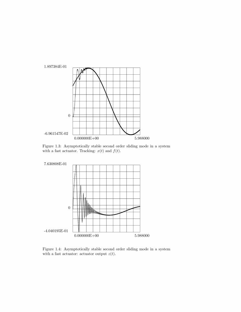
According to Section 4, the second order sliding mode is stable here with µsmall enough. Note that the last equality describes the equivalent control[35, 36, 37] and is kept actually only in the average, while the first and thesecond are kept accurately in this sliding mode.Here and further the examples are accompanied by simulation results

withf(t) = 0.08 sin t+ 0.12 cos 0.3t , x(0) = 0, z(0) = 0.

Here z is the actuator output. The plots of x(t) and f(t) with µ = 0.2are shown in Fig. 1.3, whereas the plot of z(t) is demonstrated in Fig.1.4.

Example 2. One of the main ideas of the binary system theory [8, 7] isto insert some artificial fast dynamics in the switching process. This may

0.000000E+00 5.988000-6.961547E-02

1.897384E-01

0 ```````````````````````````````````````````````````````````````````````````````````````````````````````````````````````````````````````````````````````````````````````

``````````````````````````````

`````````````````````````````````````````````````````````````````````````````````````````````````````````````````````````````````````````Figure 1.3: Asymptotically stable second order sliding mode in a systemwith a fast actuator. Tracking: x(t) and f(t).

0.000000E+00 5.988000-4.040195E-01

7.630808E-01

0 `````````````````````````````````` ```````````````````````` ``````````````````````````````````````````````````````````````````````````````````````````````````````````

```````````

Figure 1.4: Asymptotically stable second order sliding mode in a systemwith a fast actuator: actuator output z(t).

0.000000E+00 5.988000-7.492492E-02

1.941250E-01

0 ```````` `````````` ```````````` ```` `

`` ```` ````` ```` ``` ``` ``````````````````````` ```` ``````````````````````````````````` ```````````````````` ````````` ``` ````````` ``` ```` ```````

```````````````````````````````

````````````````````````````````````````````````````````````````````````````````````````````````````````````````````````````````````````Figure 1.5: Unstable second order sliding mode in a system with Aµ-controller. Tracking: x(t) and f(t).

be regarded as an installation of a fast actuator. For example, let

µz =

½ −z, |z| > |u|,−signu, |z| ≤ |u|,

where µ is a small positive number. This is a slightly modified Aµ-algorithmby Emelyanov and Korovin [8]. Having substituted u = −signσ achieve theclassical form of the algorithm with z being considered as a control.

z =

½ − 1µz, |z| > 1,− 1

µsignσ, |z| ≤ 1, (13)

Similarly to the previous example, achieve here a second order sliding modeprovided µ < 2. Simple calculation shows that the trajectories revolvearound the second order sliding manifold in coordinates t, x, z. Algorithm(13) provides for appearance of a real sliding mode of the first order withrespect to µ−1. Simulation results for µ = 0.01 are shown in Fig. 1.5, 1.6.The chattering is obvious here.

Example 3. The last actuator-like algorithm (13) may be modified inorder to receive finite time convergence to the second order sliding mode.

0.000000E+00 5.988000-1.000000

1.000000

0 `

````

`

`

`

`

`

`

``

``

`

`

`

`

`

`

`

``

``

`

`

`

`

`

`

`

``

``

`

`

`

`

`

`

`

`

`

`

`

`

`

`

``

`

`

`

`

``

`

`

`

`

``

`

`

`

``

``

`

`

`

`

``

`

`

`

`

``

`

`

`

`

``

`

`

`

``

``

`

`

`

`

``

`

`

`

`

`

`

`

``

`

`

`

`

``

`

`

`

`

``

`

`

`

`

``

`

`

`

`

``

`

`

`

`

``

`

`

`

`

`

`

`

`

`

`

`

`

`

`

``

``

`

`

`

`

`

`

`

``

``

`

`

`

``

`

``

``

`

``

`

`

`

`

`

`

`

`

`

``

`

``

``

`

``

`

`

`

`

`

`

`

``

`

``

`

`

`

`

`

`

``

``

`

`

`

`

`

``

`

`

`

`

`

`

`

`

`

`

`

``

``

`

``

``

`

`

`

`

`

`

`

`

`

`

`

`

`

`

`

`

`

`

`

`

`

`

`

`

`

`

`

``

`

`

`

`

`

`

`

`

`

`

``

``

`

`

`

`

`

`

`

``

``

`

`

`

`

`

`

`

``

``

`

`

`

`

`

`

`

``

`

`

`

`

``

`

`

`

`

``

`

`

`

`

``

``

`

`

`

``

`

`

`

`

``

`

`

`

`

``

`

`

`

`

``

`

`

`

`

``

`

`

`

`

``

`

`

`

`

``

`

`

`

`

``

``

`

`

`

`

``

`

`

`

`

``

`

`

`

``

``

`

`

`

``

`

`

`

`

``

`

``

`

`

`

`

`

`

`

Figure 1.6: Unstable second order sliding mode in a system with Aµ-controller: control z(t) (values are taken at discrete times).

The aim is gained by twisting algorithms [26, 28, 9, 10, 24]

z =

−z, |z| > 1,−5 signσ, σσ > 0, |z| ≤ 1,− signσ, σσ ≤ 0, |z| ≤ 1.

Derivative σ has to be calculated here in real time. Having substituted thefirst difference of σ for σ, achieve another version of the algorithm adaptedfor implementation:

z =

−z(ti), |z(ti)| > 1,−5 signσ(ti), σ(ti)∆σi > 0, |z(ti)| ≤ 1,− signσ(ti), σ(ti)∆σi ≤ 0, |z(ti)| ≤ 1.

Here ti ≤ ti+1. This algorithm modification constitutes a second order realsliding algorithm, which means that the sliding accuracy is proportionalto the measurement time interval squared. The corresponding simulationresults are shown in Fig. 1.7, 1.8.

Example 4. Another algorithm [12, 24] serving the same goal is the

0.000000E+00 5.988000-6.939553E-02

1.903470E-01

0 ``````````````` ````````````````````````````````````````````````````````````````````````````````````````````````````````````````````````````````````````````````````````

``````````````````````````````

`````````````````````````````````````````````````````````````````````````````````````````````````````````````````````````````````````````Figure 1.7: Second order sliding mode attracting in finite time: twistingalgorithm. Tracking: x(t) and f(t).

0.000000E+00 5.988000-1.077855E-01

3.919948E-01

0 ``````````````` ````````` `````````````````````````````````````````````````````````````````````````````````````````````````````````````

``````````````````````````````````

Figure 1.8: Second order sliding mode attracting in finite time: twistingalgorithm. Control z(t).

0.000000E+00 5.988000-6.939553E-02

1.884142E-01

0 ``````` `````````````````````````

```````````````````````````````````````````````````````````````````````````````````````````````````````````````````````````````````````

`````````````````````````````

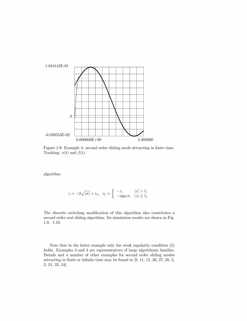
``````````````````````````````````````````````````````````````````````````````````````````````````````````````````````````````````````````Figure 1.9: Example 4: second order sliding mode attracting in finite time.Tracking: x(t) and f(t).

algorithm

z = −2p|σ|+ z1, z1 =

½ −z, |z| > 1,−signσ, |z| ≤ 1,

The discrete switching modification of this algorithm also constitutes asecond order real sliding algorithm. Its simulation results are shown in Fig.1.9, 1.10.

Note that in the latter example only the weak regularity condition (2)holds. Examples 3 and 4 are representatives of large algorithmic families.Details and a number of other examples for second order sliding modesattracting in finite or infinite time may be found in [9, 11, 12, 26, 27, 28, 2,5, 31, 32, 24].

0.000000E+00 5.988000-1.077609E-01

3.732793E-01

0 `````````````````````````````````````````````````````````````````````````````````````````````````````````````````````````````````````

````````````````````````````````````

Figure 1.10: Example 4: second order sliding mode attracting in finite time.Control z(t).

1.6 Sliding modes of order 3 and higher

Note, following [1], that for any l ≥ 3, ai,j , k 6= 0 the l-th order sliding setsin systems

y1 = y2, . . . , yl−1 = yl,yl =

Pnj=1 al,jyj + k sign y1,

yi =Pn

j=1 ai,jyj , i = l + 1, . . . , n

are always unstable with k 6= 0.This leads to an important conclusion. Even a stable high order actuator

may insert additional chattering into the closed dynamic system. Whenevera possibility of using actuators with r-th order dynamics (r > 2) for firstorder sliding mode control systems is concerned, one has to search for stableattractors of a corresponding (r + 1)-dimensional fast dynamic system oruse some special control algorithms.Example 5. Continuing the example series, let now the actuator have

second order dynamics:

z = z1, zl + 3αz1 + 2α2z = 2α2u,

where µ = 1/α → 0. Let also |f (3)(t)| < 0.5 be true. Calculation showsthat

σ(3) = −f (3)(t)− 3αz1 − 2α2z + 2α2u.

0.000000E+00 5.988000-7.370699E-02

1.925830E-01

0 ``````` ````` `` ````````````````` `` ``` `` ``````````````````` ````` `` ````````````````` ````` ``````````````````` `````````````````````````` ```````````````````````` ````````````

``````````````````````````````

`````````````````````````````````````````````````````````````````````````````````````````````````````````````````````````````````````````Figure 1.11: Unstable third order sliding mode in a system with actuatorof relative degree 2: x(t) and f(t).

It is easy to check (see Theorem 1) that, with µ <√3/3, there is a Filippov’s

solution lying on set σ = σ = σ = 0, which corresponds to the third ordersliding mode. However, it is unstable according to the classical result byAnosov [1]. Certainly, an approximation of ideal regular sliding mode isachieved with µ → 0 (Fig. 1.11). However, the actuator introduces hereconsiderable chattering (Fig. 1.12).

The following is the first published example of a third order slidingalgorithm with finite convergence time as well as of a third order slidingmode being attractive in finite time at all.Example 6. An example of a third order sliding algorithm with finite

convergence time. Define, determining by continuity when necessary,

Ψ(σ, σ) = max{0, min[1, 12+ 6(σ +

5

12|σ|2/3signσ)|σ|−2/3]},

Φ(σ, σ) =2

3(1− 2Ψ(σ, σ))(1

2|σ|3 + 1

2|σ|2) 16 .

In order not to change the notation, variable z is used below as an actualcontrol. Introduce also an auxiliary variable z1. The following algorithm

0.000000E+00 5.988000-7.211555E-01

9.999989E-01

0 ``````

`

``

`

``

``

`

`

`

`

`

`

`

``

``

`

`

``

``

`

`

`

`

`

``

``

``

`

`

``

``

`

`

`

`

`

`

`

``

``

`

`

`

``

`

`

`

`

`

`

`

``

``

`

`

`

``

`

`

`

`

`

``

``

``

`

`

``

``

`

`

`

`

`

``

``

`

`

``

``

`

`

`

`

`

`

`

``

``

`

`

``

``

`

`

`

`

`

`

`

``

``

`

`

``

``

`

`

`

`

`

`

`

``

``

`

`

``

``

`

`

`

`

`

`

`

``

``

`

`

``

``

``

`

`

`

`

`

``

``

`

`

`

``

``

``

`

`

`

``

``

`

`

``

``

`

`

`

`

`

`

`

``

``

`

`

``

``

`

`

`

`

`

`

`

``

``

`

`

``

``

`

`

`

`

`

`

`

``

``

`

`

``

``

`

`

`

`

`

`

`

``

``

`

`

``

``

`

`

`

`

`

`

`

``

``

`

`

`

`

``

``

`

`

`

``

``

`

`

`

``

``

`

`

`

`

`

``

``

`

`

`

``

`

`

`

`

`

`

`

``

``

`

`

``

``

``

`

`

`

`

`

``

``

`

`

``

``

`

`

`

`

`

``

``

``

`

`

``

``

`

`

`

`

`

``

``

`

`

`

``

``

`

`

`

`

`

``

``

`

`

``

``

`

`

`

`

`

`

`

``

``

`

`

``

``

`

`

`

`

`

`

`

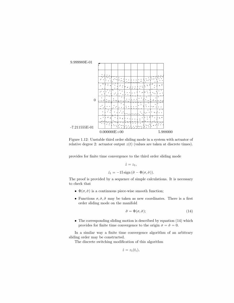
Figure 1.12: Unstable third order sliding mode in a system with actuator ofrelative degree 2: actuator output z(t) (values are taken at discrete times).

provides for finite time convergence to the third order sliding mode

z = z1,

z1 = −15 sign (σ − Φ(σ, σ)).The proof is provided by a sequence of simple calculations. It is necessaryto check that

• Φ(σ, σ) is a continuous piece-wise smooth function;• Functions σ, σ, σ may be taken as new coordinates. There is a firstorder sliding mode on the manifold

σ = Φ(σ, σ); (14)

• The corresponding sliding motion is described by equation (14) whichprovides for finite time convergence to the origin σ = σ = 0.

In a similar way a finite time convergence algorithm of an arbitrarysliding order may be constructed.The discrete switching modification of this algorithm

z = z1(ti),

0.000000E+00 9.980000-1.608659E-01

1.884106E-01

0 `````````````````````````````````````````````````````````````````````````````````````````````````````````````

``````````````````````````````````````````````````````````

`````````````````````````````````````````````````````````````````````````````````````````````````````````````

``````````````````````````````````````````````````````````Figure 1.13: Third order sliding mode attracting in finite time. Tracking:x(t) and f(t).

z1 = −15 sign (∆σ(ti)− τΦ(σ(ti), σ(ti))).

constitutes a third order real sliding algorithm providing for the slidingaccuracy being proportional to the third power of the discretization intervalτ . The simulation results are shown in Fig. 1.13, 1.14, 1.15. It wastaken that τ = 10−3, 10−4, 5 · 10−5 and the sliding precision sup |σ| =2.8 · 10−6, 1.9 · 10−9, 2.7 · 10−10 was achieved.

Note that the sliding algorithms from examples 3, 4, 6 cannot be pro-duced by the powerful differential-geometric methods by Sira-Ramirez. Atthe same time these algorithms are beyond any doubt of practical interest.One of the present authors has already successfully applied such algorithmsin solving avionics problems and constructing robust differentiators [25]. Ithas to be mentioned that these algorithms also provide for much higheraccuracy than the regular sliding modes [24].

0.000000E+00 9.980000-1.050930E-01

1.516734E-01

0 ``````````` ````````````````````` ```````````````````````````````````````

`````````````````````````````````````````````````````````````````````````````````````````````````

Figure 1.14: Third order sliding mode attracting in finite time. Controlz(t).

0.000000E+00 9.980000-1.380000E-01

2.850000E-01

0 ````````````````````` ````````````````````````````

`` ````````````````````````````` `````````````````````````````````````````````````````````````````````````````

``````````````````

Figure 1.15: Third order sliding mode attracting in finite time. Controlderivative z1(t) = z(t).

Conclusions

• Higher order sliding mode definitions were formulated.• It was shown that higher order sliding modes are natural phenomenafor control systems with discontinuous controllers if the relative degreeof the system is more than 1 or a dynamic actuator is present.

• A natural logic of actuator-like algorithm introduction was presented.Such algorithms also provide for the appearance of higher order slidingmodes.

• Stability was studied of second order sliding modes in systems withfast stable dynamic actuators of relative degree 1.

• A number of examples of higher order sliding modes were listed.Among them the first example was presented of a third order slidingalgorithm with finite time convergence. The discrete switching modi-fication of this algorithm provides for the third order sliding precisionwith respect to the minimal switching time interval.

Bibliography

[1] Anosov D.V.(1959). On stability of equilibrium points of relay systems,Automatica i telemechanica (Automation and Remote Control), 2,135-149.

[2] Chang, L.W.(1990). A MIMO sliding control with a second order slid-ing condition. ASME WAM, paper no. 90-WA/DSC-5, Dallas, Texas.

[3] DeCarlo, R.A., Zak, S.H. and Matthews, G.P. (1988). Variable struc-ture control of nonlinear multivariable systems: a tutorial. Proceedingsof the Institute of Electrical and Electronics Engineers, 76, 212-232.

[4] Drakunov, S.V. and Utkin, V.I., 1992, Sliding mode control in dynamicsystems. Int. J. Control, 55(4), 1029-1037.

[5] Elmali H. and Olgac N. (1992). Robust output tracking control of non-linear MIMO systems via sliding mode technique. Automatica, 28(1),145-151.

[6] Emelyanov, S.V., (1967) Variable Structure Control Systems, Moscow,Nauka, [in Russian].

[7] Emelyanov, S.V., (1984) Binary Systems of Automatic Control,Moscow, Institute of Control Problems, [in Russian].

[8] Emelyanov, S.V. and Korovin, S.K. (1981). Applying the principle ofcontrol by deviation to extend the set of possible feedback types. SovietPhysics, Doklady, 26(6), 562-564.

[9] Emelyanov, S.V., Korovin, S.K. and Levantovsky, L.V. (1986) Higherorder sliding modes in the binary control systems. Soviet Physics, Dok-lady, 31(4), 291-293.

[10] Emelyanov, S.V., Korovin, S.K. and Levantovsky, L.V. (1986). Secondorder sliding modes in controlling uncertain systems. Soviet Journal ofComputer and System Science, 24(4), 63-68.

29

[11] Emelyanov, S.V., Korovin, S.K. and Levantovsky, L.V. (1986). Driftalgorithm in control of uncertain processes. Problems of Control andInformation Theory, 15(6), 425-438.

[12] Emelyanov, S.V., Korovin, S.K., Levantovsky, L.V. (1990). A new classof second order sliding algorithms. Mathematical Modeling, 2(3), 89-100, [in Russian].

[13] Filippov, A.F. (1960). Differential Equations with DiscontinuousRight-Hand Side. Mathematical Sbornik, 51(1), 99-128 [in Russian].

[14] Filippov, A.F. (1988). Differential Equations with DiscontinuousRight-Hand Side. Kluwer, Dordrecht, the Netherlands.

[15] Fridman, L.M. (1983). An analogue of Tichonov’s theorem for onekind of discontinuous singularly perturbed systems. In: ApproximateMethods of differential equations research and applications. KuibyshevUniversity press., 103-109 (in Russian)

[16] Fridman, L.M. (1985) On robustness of sliding mode systems with dis-continuous control function, Avtomatica i Telemechanica (Automation& Remote Control), 5, 172 -175 (in Russian).

[17] Fridman, L.M. (1986) Singular extension of the definition of discon-tinuous systems, Differentialnye uravnenija (Differential equations), 8,1461-1463 (in Russian).

[18] Fridman, L.M. (1990) Singular extension of the definition of discontin-uous systems and stability, Differential equations, 10, 1307-1312.

[19] Fridman, L.M. (1991) Sliding Mode Control System Decomposition,Proceedings of the First European Control Conference, Grenoble, 1,13-17.

[20] Fridman, L.M. (1993) Stability of motions in singularly perturbed dis-continuous control systems Prepr.of XII World Congress IFAC, Sydney,4, 367-370.

[21] Fridman, L.M., Shustin E., Fridman E. (1992) Steady modes in dis-continuous equations with time delay, Proc. of IEEE Workshop Vari-able Structure and Lyapunoff Control of Uncertain Dynamic Systems,Sheffield, 65-70.

[22] Isidory, A.(1989). Nonlinear Control Systems. Second edition, SpringerVerlag, New York.

[23] Itkis, U., 1976, Control Systems of Variable Structure, Wiley, NewYork.

[24] Levant A. (Levantovsky, L.V.) (1993) Sliding order and sliding accu-racy in sliding mode control. International Journal of Control, 58(6),1247-1263.

[25] Levant A.(1993) Higher order sliding modes. In ”International Confer-ence on Control Theory and Its Applications: Scientific Program andAbstracts”, Kibbutz Maale HaChamisha, Israel, 84-85.

[26] Levantovsky, L.V. (1985). Second order sliding algorithms: their real-ization. In ”Dynamics of Heterogeneous Systems”, Institute for SystemStudies, Moscow, 32-43 [in Russian].

[27] Levantovsky, L.V. (1986). Sliding modes with continuous control. In”Proceedings of the All-Union Scientific-Practical Seminar on Applica-tion Experience of Distributed Systems, I. Novokuznezk, USSR, 1986”,79-80, Moscow [in Russian].

[28] Levantovsky, L.V. (1987). Higher order sliding modes in the systemswith continuous control signal. In ”Dynamics of Heterogeneous Sys-tems”, Institute for System Studies, Moscow, 77-82 [in Russian].

[29] Saksena, V.R., O’Reilly, J. and Kokotovic, P.V., 1984, Singular Pertur-bations and Time-Scale Methods in Control Theory. Survey 1976-1983,Automatica 20(3), 273-293.

[30] Sira-Ramirez, H. (1992). On the sliding mode control of nonlinear sys-tems. Systems & Control Letters, 19, 303-312.

[31] Sira-Ramirez, H. (1992). Dynamical sliding mode control strategies inthe regulation of nonlinear chemical processes. International Journalof Control, 56(1), 1-21.

[32] Sira-Ramirez, H. (1993). On the dynamical sliding mode control ofnonlinear systems. International Journal of Control, 57(5), 1039-1061.

[33] Slotine, J.-J. E., and Sastry, S.S. (1983). Tracking control of non-linearsystems using sliding surfaces, with applications to robot manipulators.International Journal of Control, 38, 465-492.

[34] Su W.-C., Drakunov S., Ozguner U. (1994). Implementation of vari-able structure control for sampled-data systems. Proceedings of IEEEWorkshop on Robust Control via Variable Structure & Lyapunov Tech-niques, Benevento, Italy (1994), 166-173.

[35] Utkin, V.I. (1977). Variable structure systems with sliding modes: asurvey. IEEE Transactions on Automatic Control, 22, 212-222.

[36] Utkin, V.I. (1981). Sliding Modes in Optimization and Control Prob-lems. Nauka, Moscow [in Russian].

[37] Utkin, V.I. (1992). Sliding Modes in Optimization and Control Prob-lems, Springer Verlag, New York.

[38] Young, K.K.D., Kokotovic, P.V. and Utkin, V.I., 1977, A singular per-turbation analysis of high-gain feedback systems. IEEE Transactionson Automatic Control, 22, 931-938.

[39] Zinober, A.S.I., (editor), (1990). Deterministic Control of UncertainSystems, Peter Peregrinus, London.