higher-order whep solutions of quadratic nonlinear...

Engineering, 2013, 5, 57-69 http://dx.doi.org/10.4236/eng.2013.55A009 Published Online May 2013 (http://www.scirp.org/journal/eng)

Higher-Order WHEP Solutions of Quadratic Nonlinear Stochastic Oscillatory Equation

Mohamed A. El-Beltagy1, Amnah S. Al-Johani2,3 1Department of Engineering Mathematics & Physics, Engineering Faculty, Cairo University, Giza, Egypt

2Department of Applied Mathematics, College of Science, Northern Borders University, Arar, KSA 3College of Home Economics, Northern Borders University, Arar, KSA

Email: [email protected], [email protected]

Received February 25, 2013; revised March 28, 2013; accepted April 7, 2013

Copyright © 2013 Mohamed A. El-Beltagy, Amnah S. Al-Johani. This is an open access article distributed under the Creative Com-mons Attribution License, which permits unrestricted use, distribution, and reproduction in any medium, provided the original work is properly cited.

ABSTRACT

This paper introduces higher-order solutions of the quadratic nonlinear stochastic oscillatory equation. Solutions with different orders and different number of corrections are obtained with the WHEP technique which uses the Wiener- Hermite expansion and perturbation technique. The equivalent deterministic equations are derived for each order and correction. The solution ensemble average and variance are estimated and compared for different orders, different number of corrections and different strengths of the nonlinearity. The solutions are simulated using symbolic computa- tion software such as Mathematica. The comparisons between different orders and different number of corrections show the importance of higher-order and higher corrected WHEP solutions for the nonlinear stochastic differential equations. Keywords: Oscillatory Equation; Nonlinear Differential Equations; Stochastic Differential Equation; Wiener-Hermite

Expansion; Perturbation Technique

1. Introduction

Analysis of the response of linear and nonlinear systems subjected to random excitations is of considerable inter- est to the fields of mechanical and structural engineering [1]. Stochastic differential equations based on the white noise process provide a powerful tool for dynamically modeling complex and uncertain aspects. In many prac- tical situations, it is appropriate to assume that the nonlinear term affecting the phenomena under study is small enough; then its intensity is controlled by means of a frank small parameter, say [2].

According to [3], the solution of stochastic partial differential equations (SPDEs) using Wiener-Hermite expansion (WHE) has the advantage of converting the problem to a system of deterministic equations that can be solved efficiently using the standard deterministic numerical methods. The main statistics, such as the mean, covariance, and higher order statistical moments, can be calculated by simple formulae involving only the deterministic Wiener-Hermite coefficients. In WHE approach, there is no randomness directly involved in the computa- tions. One does not have to rely on pseudo random number generators, and there is no need to solve the stochas-

tic PDEs repeatedly for many realizations. Instead, the deterministic system is solved only once.

The application of the WHE [4-10] aims at finding a truncated series solution to the solution process of a stochastic differential equation. The truncated series com- poses of two major parts; the first is the Gaussian part which consists of the first two terms, while the rest of the series constitute the non-Gaussian part. In non-linear cases, there exists always difficulties of solving the resultant set of deterministic integro-differential equations got from the applications of a set of comprehensive averages on the stochastic integro-differential equation obtained after the direct application of WHE. Many authors introduced different methods to face these obstacles. Among them, the WHEP technique [4] was introduced using the perturbation technique to solve perturbed nonlinear problems.

The WHE was originally started and developed by Norbert Wiener in 1938 and 1958 [11]. Wiener con- structed an orthonormal random bases for expanding ho- mogeneous chaos depending on white noise, and used it to study problems in statistical mechanics. Cameron and Martin [12] developed a more explicit and intuitive formulation for Wiener-Hermite expansion (now it is known

Copyright © 2013 SciRes. ENG

M. A. EL-BELTAGY, A. S. AL-JOHANI 58

as Wiener Chaos Expansion, WCE). Their development is based on an explicit discretization of the white noise process through its Fourier expansion, which was missed in Wiener’s original formalism. This approach is much easier to understand and more convenient to use, and hence replaced Wiener’s original formulation. Since Ca- meron and Martin’s work, WHE has become a useful tool in stochastic analysis involving white noise (Brow- nian motion) [3]. Also, another formulation was sug- gested and applied by Meecham and his co-workers [13, 14]. They have developed a theory of turbulence involving a truncated WHE of the velocity field. The randomness is taken up by a white-noise function associated, in the original version of the theory, with the initial state of the flow. The mechanical problem then reduces to a set of coupled integro-differential equations for deterministic kernels. In [1], the WHE (Imamura formulation, [13]) was used to compute the nonstationary random vibration of a Duffing oscillator which has cubic nonlinearity under white-noise excitation. Solutions up to second order are obtained by solving the equivalent deterministic system by an iterative scheme. M. El-Tawil and his co- workers [4-10] used the WHE together with the perturbation theory (WHEP technique) to solve a perturbed nonlinear stochastic diffusion equation.

As in [15], the analysis of nonlinear random vibration has been studied using several methods, such as, equivalent linearization method [16], stochastic averaging method [17], the WHE approach with nonstationary excitations [1], the WHE method combining with the small perturbation technique [18], eigenfunction expansions [19], and the method of detailed balance [20]. All the above methods are applied and used for nonlinear random oscillations of real systems subjected to random nonstationary (or stationary) excitations.

As in [5,6], quadrate oscillation arises through many applied models in applied sciences and engineering when studying oscillatory systems [21]. These systems can be exposed to a lot of uncertainties through the external forces, the damping coefficient, the frequency and/or the initial or boundary conditions. These input uncertainties cause the output solution process to be also uncertain. For most of the cases, getting the probability density function (p.d.f.) of the solution process may be impossi- ble. So, developing approximate techniques (through which approximate statistical moments can be obtained) is an important and necessary work. There are many techniques which can be used to obtain statistical moments of such problems. The main goal of this paper is to compare some of these methods when applied to a quadrate nonlinearity problem.

In [22], the WHEP technique is generalized to nth nonlinearity, general order of WHE and general number of corrections. Also, the extension to handle white noise

in more than one variable and general nonlinearities are outlined. The generalized algorithm is implemented and linked to MathML [23] script language to print out the resulting equivalent deterministic system.

In the current work the generalized WHEP technique developed in [22] is used to derive higher-order with higher corrections system of equations for the quadratic nonlinear stochastic oscillatory equation and then solve them. Up to fourth order equations are derived with different number of corrections. The mean and variance of the response will be simulated up to third order using Mathematica.

This paper is organized as follows. The formulation of the quadratic nonlinear stochastic oscillatory equation is outlined in Section 2. The WHEP technique is reviewed in Section 3. The equivalent deterministic system is derived in Section 4. In Section 5, the mean and variance of the solution is simulated with different order, different number of corrections and different values of the nonlinearity strengths.

2. Problem Formulation

In this paper, the nonlinear oscillatory equation:

2 ; 0,nL x t x f t g t N t t T (1)

is considered under stochastic excitation and with the proper set of initial conditions

0 00 and 0 0x x x x which is assumed to be deterministic. The operator L is a general linear operator and in the case of the oscillatory equation it will be:

22

2

d d2

ddL

tt

where is the undamped angular frequency of the oscillator and is the damping ratio. The nonlinearity is introduced as losses of degree strengthened by a deterministic small parameter

1n . The uncertainty is

introduced through white noise scaled by a deterministic envelope function g t . The white noise is considered here as a function of time but it can be generalized in time and space as it was declared in [22]. The function f t is a deterministic forcing function. Theorem (1)

will be used in the derivation of the WHEP technique. Theorem (1): The solution of Equation (1), if exists, is

a power series in , i.e.

0

ii

i

x t x

t (2)

The theorem can be proved using the mathematical induction with the Pickard iterative technique [22]. As a direct result of this theorem, it is expected that the average, the variance as well as the covariance are also power series of .

The WHEP technique will be used in this work to de-



te

3. WHEP Technique

ompleteness of the Wiener-

rmine the equivalent deterministic set of equations. The deterministic equations are then solved to obtain the solution kernels and hence the mean and variance of the response.

The average of almost all Wiener-Her ite functionals vanishes, particularly,

The expectation and variance of the solution will be:

m

As a consequence of the cHermite set [13], any arbitrary stochastic process can be expanded in terms of the Weiner-Hermite polynomial set and this expansion converges to the original stochastic process with probability one.

The solution function ;x t w can be expanded in te

Or after eliminating the parameters, for the sake of br

d

rms of Wiener-Hermite functionals as [4]:

x t w

0 1 11 1 1

2 21 2 1 2 1 2

3 31 2 3 1 2 3 1 2 3

;

; ; d

; , , ; d d

; , , , , ; d d d

x t x t t H t w t

x t t t H t t w t t

x t t t t H t t t w t t t

evity, we get:

0

1

,;k

k kk

k R

x t w x t x H

(3)

where 1 2d d d dk kt t t and is a k-dimensional

integral ver the variables The first term in n-random

kR

o 1 2, , , kt t t .

the expansion (3) is the no part or ensemble mean of the function. The first two terms represent the normally distributed (Gaussian) part of the solution. Higher terms in the expansion depart more and more from the Gaussian form. The Gaussian approximation is usually a bad approximation for nonlinear problems, especially when high order statistics are concerned [3].

The components ; , , ,j1 2 jx t t t t are called the

(deterministic) kernels of the WHE for x t . The variable w is a random output of a triple probability space , ,B P , where is a sample space, B is a -

sociated w h and P is a probability meas- ure. For simplicity, w w l be dropped later on.

The functional 1 2, , ,nn

algebra as itil

H t t t is the thn order Wiener-Hermite tim nctional. e Wie- ner-H functionals form a complete set with 0 1

e-independent fu ThH

and 11 1H t N t : the white noise. By cons

the W unctions are symmetric in their ar- guments and are statistically orthonormal, i.e.

i j

truction,iener-Hermite f

0, .E H H i j

0, 1iE H i

m

0

2

1

Var ! dk

ki k

k R

E x t x t

x t k x

(4)

The WHE method can be elementary used istochastic differential equations by expanding the solu- tio

n solving

n as well as the stochastic input processes via the WHE. The resultant equation is more complex than the original one due to being a stochastic integro-differential equation [4]. Taking a set of ensemble averages together with using the statistical properties of the WHE functionals, a set of deterministic integro-differential equations are obtained in the deterministic kernels

1 2; , , , ; 0,1, 2, .iix t t t t i To obtain approximate

solutions of these deterministic kernels, one can use pertur having a perturbed system depending on a small parameter

bation theory in the case of . Expanding the ker-

nels as a power series of , another set of simpler iterative equations in the kernel series components are obtained. This is the main idea of the WHEP algorithm.

The WHEP technique for general nonlinear exponent n , general order m and general number of corrections NC follow the steps [22]:

1. Truncate the e pansion (3) to contain only x 1, 1mm kernels ;0jx j m , i.e.

0 ;; dk km

t w x t x H1 kk R

kx and then

2. Substitute into the stochasti ifferential Equation (1);

c partial d

3. Use the multinomial theorem to expand the nonlinear term nx in (1);

4. Multiply by ;0jH j m and then apply the ensemble average. This will lead to 1m equations

the kernels ;0jx j m ; in

5. For each kernel ;0jx j m , the pertur- apply e up to i.e. bation techniqu NC corrections,

0

NCj ji

ii

x x

;

6. Equating t coefficients of in both sides to get

he ;0k k NC 1NC equations for each kernel

;0jx j m . This will l the following 1 1m NC equa-

tead to

ions [22]:

! jj L x f t 00 1

0

j j t

j

t tg

m

1 ;

(5)



, 1!

0 ,1

j j ;jb f f b

f

j L x c D E

j m b NC

f

where

(6)

, 1

var 0 0

dpg

z

m NC hj if b g p

i pR

D c x z

(7)

And the expectations jfE are computed as:

0

jf

m kj ij

fi

E H H

(8)

It was explained in [22] how to get jfE in terms of

the Dirac delta functions and then use

integrals appear in

them to reduce the

, 1j

f bD . The summation means var

that all variations ;0 ,0pqh q m p NC that satisfy

m NC

the equality 0 0

pqd p are selected. Th an be

q p h is c

g technique. For these vdone be a searchin ariations, the

factors

0

!

!if

NCgpg

p

h

k will bec multiplied by each other to

get g

c i.e. var

g gc c . The term 0j is the Kronecker

wise ilarly 1

delta function that equals one when and zero other- . Sim , the term

0j j is the Kron er delta

func hat equal en 1j and zer herwise. The counter

ecktion t s one w o oth

f , in the su right hand side

er

mmation in the

of (6), runs over all the n m

combinations of the

positive integ s 0 1, , , m

n

f f fk k k such that 0

mif

i

k n

.

Equations (5) and (6) ca s be solved using the

solved independen ;0

n alwayproper sequence. The first Equations (5) are

tly to get 1m

0

jx j m used to compute t ponents in (6

om

then they are he other c ). For 0j ,

the component 00u is obtained by solving

00 al iniL x f t with the origin tial conditions which

are assumed deterministic. For 1j , the component 10x is obtained solving by 1

0 g tL x t t 1 with

zero initial conand sid

fy the solutito b

ditions. The other components 0 ; 2jx j

will be zeros due to zero right h e and zero initial conditions. Equations (6) speci on sequence

e followed. The component jix is ev

f the previously computed c entsaluated in

terms o

ompon; ,p

kx p j k i . This means that the 1st corre all kernels,

1 ;0jctions for

x j m are solved firstly then solv-

ing the 2nd corrections for all kernels, 2 ;0j

x j m ,

up to the thNC corrections for kernels ;0jNC

all x j m .

These resultsg WHE. In W

e bottom, thrcing di

rectly we inant in

are consistent with the known results obtained usin HE, higher order kernels are driven by lower order kernels, and at th e Ga els a - ussian kern re driven by the random fo

. So, the r order kernels are usually dom lo magnitude [3]. The statistical properties of the solution will now be

calculated as:

0

0

NCi

ii

E x t x

Var ! dm NC

kii kx t k x

2

1 0kk iR

(9)

If

0

j jii

i

x x

, then it will be convergent if [22]:

1

ji

ji

x

x

for 0 ,Tt t means that . This should obey an up- pe ition after which divergence is obtained.

The formulation given in Equations (5) and (6) are quite general and could be used or analysis of the response of an any linear operator with degree non-

r bound cond

fL

rar

thnlinearity and subjected to an arbit y, stationary, or nonstationary Gaussian or non-Gaussian random excitation.

Consider the quadratic 2n nonlinear oscillatory equation with excitation function:

2 2 22x x x f (10)

With the initial conditions

x t

0 0 00 and 0x x x x

In case of zero initial conditions,

the exact solution can be obtained using different methods such as lin Laplace transform, an

the theory of ear differential equations or thed it will be the convolution:

0

dt

x t h t f t h t f (11)

where 1e sint

dd

h t t

with 21d ,

which is the angular frequency of the underdamped 1 harmonic oscillator.

For e tf t , the solution will results in:

2

1

1 2

e sin d

t

t

1

e e cost t td t

d

x



The solution (11) of the model Equation (10) can be used as a model solution that is used in all kernels after considering the proper right hand side for the nel equation.

4.

ar oscillatory equation and first order (m = 1) rrec-

deter-

ker

The Equivalent Deterministic System

Applying the above mentioned WHEP algorithm to get the following systems of equations of the quadratic (n = 2) nonlineGaussian approximation and different number of cotions NC . The initial conditions are assumed ministic and hence only the zero-order and zero-

correction kernel equation 00L x f t will has the

initial conditions 0 0andx x . Other kernels equations

will have zero initial conditions. 1NC :

0

1

0

0 0 12 21 0 0 1

1 0 121 0 0 1

d

2

R

L x f t

L x g t t t

L x x x t t

L x x x t

0 1

2 2

1

: The above equations in addition to:

d


2NC

0 0 0 1 12 22 0 1 0 1 1 1 1

1 0 1 0 12 22 0 1 1 1 0 1

2 2

2 2

R

L x x x x t x t t

L x x x t x x t

3NC

20 0 0 02 2

3 0 2 1

21 1 12 2

0 1 2 1 1 1 1 1

1 0 1 0 12 23 0 2 1 1 1 1

0 122 0 1

2

2 d

2 2

2

L x x x x

R R

dx t x t t x t t

L x x x t x x t

x x t

4NC : The above equations in addition to:

0 0 0 0 02 24 0 3 1 2

0 121 1 3 1 1

1 1 2 1 1

1 0 1 0 12 24 0 3 1 1 2

0 1 0 12 22 1 1 3 0 1

2 2

2 d

2 d

2 2

2 2

R

L x x x x x

x t x t t

x t x t t

L x x x t x x t

1

1 12

R

x x t x x t


20 0 0 0 02 2 25 0 4 1 3

1 120 1 4 1 1

1 121 1 3 1 1

2122 1 1

15 0 4 1 1 3 1

0 1 0 12 22 2 1 3 1 1

0 124 0 1

2 2

2 d

2 d

d

2 2

2 2

2

R

R

R

L x x x x x x

x t x t t

x t x t t

x t t

L x x x t x x t

x x t x x t

x x t

0 1 0 12 2

02

In case of zero initial conditions and zero deterministic excitation [i.e. 0

0 0x ], we shall have:

00

10 1

20 121 0 1 1

1

2

1 0 122 1 0 1

20 0 1 12 2

3 1 0 1 2 1

13

04

1 0 1 0 12 24 1 2 1 3 0 1

0 0 0 1 12 25 1 3 0 1 4 1

2122 1 1

0

d

0

0

2

2 d

0

0

2 2

2 2

d

R

R

R

R

L x

L x g t t t

L x x t t

L x

L x

L x x x t

L x x x t x t t

L x

L x

L x x x t x x t

L x x x x t x t t

x t t

L x

15 0

1

1

1d

Which means the all of

0

0 1 0 1 10 1 2 3 5, , , ,x x x x x and

00x are become zeros. The second order 2m equations will be:

1NC :



00

10 1

20

2 20 0 12 2

1 0 0 1

1 0 121 0 0 1

2 1 121 0 1 0 2

2 0

d

2

2 2

R

L x f t

L x g t t t

L x

L x x x t t

L x x x t

L x x t x t

1


1

2


2NC

0 0 0 1 12 22 0 1 0 1 1 1

1 0 1 0 12 22 0 1 1 1 0 1

1 220 2 1 1 2 2

2 0 2 1 12 22 0 1 1 2 0 1 1

2 2 d

2 2

4 , d

2 4 , 4

R

R

L x x x x t x t t

L x x x t x x t

x t x t t t

L x x x t t x t x t

3NC

2

20 0 0 02 23 0 2 1

1 120 1 2 1 1

1

21 1 2 1 2

1 0 1 0 12 23 0 2 1 1 1 1

0 122 0 1

1 220 2 2 1 2 2

1 221 2 1 1 2 2

2 0 22 23 0 2 1 2

2

2 d

d

2 , d d

2 2

2

4 , d

4 , d

2 4 , 4

R

R

R

R

L x x x x

x t x t t

t

x t t t t

L x x x t x x t

x x t

x t x t t t

x t x t t t

L x x x t t x

212

1 1R

x t

22

0 21 1 1 2

1 120 1 2 2

1 1 1 2

2 221 1 3 1 2 3 3

,

4

2

8 , , dR

1 12

x t t

x t x t

x t x t

x t t x t t t

4NC

2

0 0 0 0 02 24 0 3 1 2

1 120 1 3 1 1

1 121 1 2 1 1

2 221 1 2 2 1 2 1 2

1 0 1 0 12 24

0 1 0 12 22 1 1 3 0 1

1 220 2 3 1 2 2

1 221 2 2 1 2 2

1 222 2 1

2

2 d

2 d

4 , , d d

2 2

2 2

4 , d

4 , d

4

R

R

R

R

R

L x x x x x

x t x t t

x t x t t

x t t x t t t t

L x x x t x x t

x x t x x t

x t x t t t

x t x t t t

x t x

0 3 1 1 2 1

1 2 2

2 0 2 0 22 24 0 3 1 2 1 2

0 2 1 12 22 1 1 2 0 1 3 2

1 121 1 2 2

2 221 1 3 2 2 3 3

, d

2 4 , 4

4 , 4

4

8 , , d

R

R

t t t

L x x x t t x x t t1 2,

x x t t x t x t

x t x t

x t t x t t t

3m equations are: The third order 1NC :

00

10 1

20

30

2 20 0 12 21 0 0 1

1 0 121 0 0 1

1 0 1 0 2

31

2 0

6 0

d

2

2 2

6 0

R

L x f t

L x g t t t

L x

L x

L x x x t t

L x x x t

L x x t x t

L x

1

2 1 12


0 0 0 1 12 22 0 1 0 1 1 1 1

1 0 1 0 12 22 0 1 1 1 0 1

1 220 2 1 1 2 2

2 0 2 1 12 22 0 1 1 2 0 1 1

3 1 222 0 1 1 2 3

2 2 d

2 2

4 , d

2 4 , 4

6 12 ,

R

R

L x x x x t x t t

L x x x t x x t

x t x t t t

L x x x t t x t x t

L x x t x t t

2





2

20 0 0 02 2

3 0 2 1

1 120 1 2 1 1

2121 1 1

222

1 1 2 1 2

1 0 1 0 12 23 0 2 1 1 1 1

0 1 1 22 22 0 1 0 2 2 1 2 2

1 221 2 1 1 2 2

2 0 22 23 0 2 1 2

2

2 d

d

2 , d d

2 2

2 4 ,

4 , d

2 4 , 4

R

R

R

R

R

L x x x x

x t x t t

x t t

x t t t t

L x x x t x x t

dx x t x t x t t t

x t x t t t

L x x x t t x

0 21 1 1 2

1 1 1 12 20 1 2 2 1 1 1 2

2 221 1 3 1 2 3 3

3 0 322

1 220 1 2 2 3

1 221 1 1 2 3

,

4 2

8 , , d

6 1

12 ,

12 ,

R

x t t

x t x t x t x t

x t t x t t t

x x

x t x t t

x t x t t

3 0 1 2 32 , ,L x t t t


2

0 0 0 0 02 24 0 3 1 2

1 120 1 3 1 1

1 121 1 2 1 1

2 221 1 2 2 1 2 1 2

2

2 d

2 d

4 , , d

R

R

R

L x x x x x

x t x t t

x t x t t

dx t t x t t t t

2

1 0 1 0 12 24

2 1 1 3 0 1

1 220 2 3 1 2 2

1 221 2 2 1 2 2

1 222 2 1 1 2 2

2 321 2 3 2 1 2 3 2 3

2 2

2 2

4 , d

4 , d

4 , d

12 , , d, d

R

R

R

R

L x x x t x x t

x x t x x t

x t x t t t

x t x t t t

x t x t t t

0 3 1 1 2 1

0 1 0 12 2

x t t x t t t t t

2 0 2 0 22 24 0 3 1 2 1 2

0 2 1 12 22 1 1 2 0 1 3 2

1 121 1 2 2

1 320 3 3 1 2 3 3

1 321 3 3 1 2 3 3

2 22

2 222 1 3 1 2 3 3

2 4 , 4

4 , 4

4

12 , d

12 , d

8 , , d

8 , , d

,

,

R

R

R

L x x x t t x x t t1 2,

1 1 3 2 1 2 3R

x x t t x t x t

x t x t

x t x t t t t

x t x t t t t

x t t x t t t

x t t x t t t

3 0 324 0 3 1 2 3

0 321 2 1 2 3

1 220 1 3 2 3

1 221 1 2 2 3

1 222 1 1 2 3

2 321 1 4 2 2 3 4 4

2 321 2 4 2 1 3 4 4

2 321 3 4 2 1 2 4 4

6 12 , ,

12 , ,

12 ,

12 ,

12 ,

24 , , , d

24 , , , d

24 , , , d

R

R

R

L x x x t t t

x x t t t

x t x t t

x t x t t

x t x t t

x t t x t t t t

x t t x t t t t

x t t x t t t t

4m equations are: The fourth order 1NC :

00

10 1

20

30

4

2 20 0 12 21 0 0 1

1 0 121 0 0 1

2 1 121 0 1 0 2

31

41

2 0

6 0

24

d

2

2 2

6 0

24 0

R

L x f t

L x g t t t

L x

L x

L x x x t t

L x x x t

L x x t x t

L x

L x

0 0L x

1




0 0 0 1 12 22 0 1 0 1 1 1 1

1 0 1 0 12 22 0 1 1 1 0 1

1 220 2 1 1 2 2

2 0 2 1 12 22 0 1 1 2 0 1 1

3 1 222 0 1 1 2 3

42

2 2 d

2 2

4 , d

2 4 , 4

6 12 ,

24 0

R

R

L x x x x t x t t

L x x x t x x t

x t x t t t

L x x x t t x t x t

L x x t x t t

L x

2

5. Results

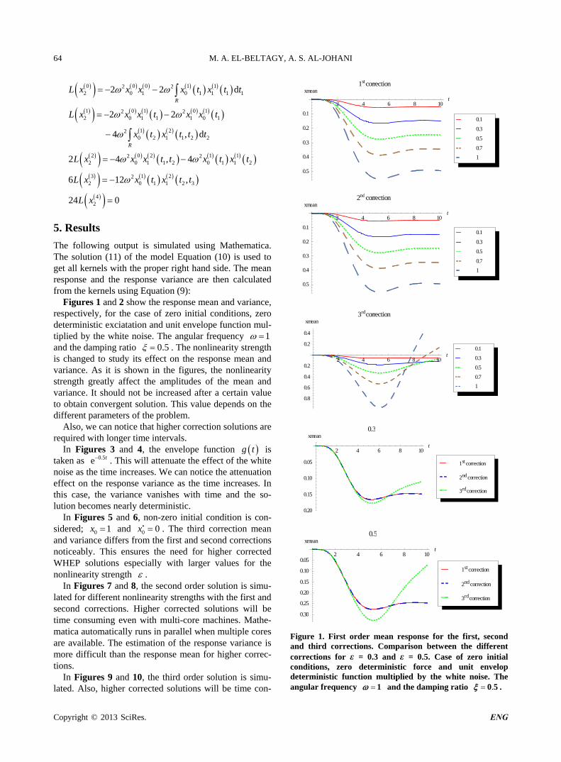
The following output is simulated using Mathematica. The solution (11) of the model Equation (10) is used to get all kernels with the proper right hand side. The mean response and the response variance are then calculated from the kernels using Equation (9):

Figures 1 and 2 show the response mean and variance, respectively, for the case of zero initial conditions, zero deterministic exciatation and unit envelope function multiplied by the white noise. The angular frequency 1 and the damping ratio 0.5 . The nonlinearity strenis changed to study its effect on the response mean and variance. As it is shown in the figures, the nonlinearity strength greatly affect the amplitudes of the mean and variance. It should not be increased after a certain value to obtain convergent solution. This value depends on the different parameters of the problem.

Also, we can notice that higher correction solutions are required with longer time intervals.

In Figures 3 and 4, the envelope function

gth

g the wh

ten

is taken as . This will attenuate the effect of t ite noise as t e time increases. We can notice the at n effect on the response variance as the time increases. In this case, the variance vanishes with time and the solution becomes nearly deterministic.

In Figures 5 and 6, non-zero initial condition is considered; and . The third correction mean and varia ffers first and second corrections noticeably. This ens need for higher corrected W es for the nonlinea rength

0.5e t

h uatio

0 1x nce di

ri st

0 0x

from the ures thepeciallyHEP solutions es with larger valu

ty .

2 4 6 8 10t

0.5

0.4

0.3

0.2

0.1

xmean1stcorrection

1

0.7

0.5

0.3

0.1

2 4 6 8 10t

0.5

0.4

0.3

0.2

0.1

xmean2ndcorrection

1

0.7

0.5

0.3

0.1

2 4 6 8 10t

0.8

0.6

0.4

0.2

0.2

0.4

xmean3rdcorrection

1

0.7

0.5

0.3

0.1

2 4 6 8 10t

xmean0.3

In Figures 7 and 8, the second order solution is simulated for different nonlinearity strengths with the first and second corrections. Higher corrected solutions will be time consuming even with multi-core machines. Mathe- matica automatically runs in parallel when multiple cores are available. The estimation of the response variance is more difficult than the response mean for higher corrections.

In Figures 9 and 10, the third order solution is simulated. Also, higher corrected solutions will be time con-

0.20

0.15

0.10

1stcorrection0.05

2ndcorrection

3rdcorrection

2 4 6 8 10t

0.30

0.25

0.20

0.15

0.10

0.05

xmean0.5

3rdcorrection

2ndcorrection

1stcorrection

Figure 1. First order mean response for the first, second and third corrections. Comparison between the different corrections for ε = 0.3 and ε = 0.5. Case of zero initial conditions, zero deterministic force and unit envelop deterministic function multiplied by the white noise. The

gular frequency an 1 and the damping ratio . 0 5 .



2 4 6 8 10t

0.20

0.25

0.30

0.35

0.40

0.45

50

xvar1stcorrection

0.

1

0.7

0.5

0.3

0.1

0 2 4 6 8 10t

1

2

3

4

5xvar

2ndcorrection

1

0.7

0.5

0.3

0.1

2 4 6 8 10t

0.5

1.0

1.5

2.0

xvar3rdcorrection

1

0.7

0.5

0.3

0.1

0 2 4 6 8 10t

0.1

0.2

0.3

0.4

0.5

0.6

0.7xvar

　　0.3

3rdcorrection

2ndcorrection

1stcorrection

0 2 4 6 8 10t

0.2

0.4

0.6

0.8

1.0

1.2

1.4

xvar　　0.5

3rdcorrection

2ndcorrection

1stcorrection

Figure 2. First order response variance for the first, second and third corrections. Comparison between the different corrections for ε = 0.3 and ε = 0.5. Case of zero initial conditions, zero deterministic force and unit envelop

eterministic function multiplied by the white noise. The ngular frequency

da 1

2 4 6 8 10t

0.15

0.10

0.05

xmean1stcorrection

1

0.7

0.5

0.3

0.1

2 4 6 8 10t

0.15

0.10

0.05

xmean2ndcorrection

1

0.7

0.5

0.3

0.1

2 4 6 8 10t

and the damping ratio .0 5 .

0.25

0.20

0.15

0.10

0.05

xmean3rdcorrection

0.3

0.5

0.7

1

0.1

2 4 6 8 10t

0.06

0.05

0.04

0.03

0.02

0.01

0.01xmean

0.3

3rdcorrection

2nd correction

1stcorrection

2 4 6 8 10t

0.08

0.06

0.04

0.02

xmean0.5

3rdcorrection

2ndcorrection

1stcorrection

Figure 3. First order mean response for the first, second and third corrections. Comparison between the different corrections for ε = 0.3 and ε = 0.5. Case of zero initial conditions, zero deterministic force and envelop deterministic function multiplied by the e noise. Thangular frequency

. t0 5e whit e

1 and the dampi o ng rati .0 5 .



2 4 6 8 10t

0.05

0.10

0.15

0.20xvar

1stcorrection

1

0.7

0.5

0.3

0.1

2 4 6 8 10t

0.05

0.10

0.15

0.20

xvar2ndcorrection

1

0.7

0.5

0.3

0.1

2 4 6 8 10t

0.05

0.10

0.15

0.20

xvar3rdcorrection

1

0.7

0.5

0.3

0.1

0 2 4 6 8 10t

0.05

0.10

0.15

0.20xvar

　　0.3

3rdcorrection

2ndcorrection

1stcorrection

0 2 4 6 8 10t

0.05

0.10

0.15

0.20xvar

　　0.5

3rdcorrection

2nd correction

1st correction

Figure 4. First order response variance for the first, second and third corrections. Comparison between the different corrections for ε = 0.3 and ε = 0.5. Case of zero initial

conditions, zero deterministic force and envelop deterministic function multiplied by the w ise. The angular frequency

. t0 5ehite no

1 and the damping ratio .0 5 .

2 4 6 8 10t

1.0

0.5

0.5

1.0

xmean1stcorrection

1

0.7

0.5

0.3

0.1

2 4 6 8 10t

3

2

1

1

xmean2ndcorrection

1

0.7

0.5

0.3

0.1

2 4 6 8 10t

10

8

6

4

2

2xmean

3rdcorrection

0.1

0.3

0.5

0.7

1

2 4 6 8 10t

　0.5

0.5

1.0

xmean0.3

3rdcorrection

2ndcorrection

1stcorrection

2 4 6 8 10t

2.0

1.5

1.0

0.5

0.5

1.0

xmean0.5

3rdcorrection

2nd correction

1stcorrection

Figure 5. First order mean response for the first, second and third corrections. Comparison between the different corrections for ε = 0.3 and ε = 0.5. Case of initial conditions

and 0 0x 0 1x , zero deterministic force and unit

dete nction multiplied by the white noise. gu ncy

envelopThe an

rministic fular freque 1 and the damping ratio

.0 5 .



0 2 4 6 8 10t

5

10

15

20xvar

1stcorrection

1

0.7

0.5

0.3

0.1

0 2 4 6 8 10t

10

20

30

40

50xvar

2ndcorrection

1

0.7

0.5

0.3

0.1

0 2 4 6 8 10t

50

100

150

200

250

300xvar

3rdcorrection

1

0.7

0.5

0.3

0.1

2 4 6 8 10t

0.5

1.0

1.5

2.0

2.5

xvar　　0.3

3rd correction

2ndcorrection

1stcorrection

2 4 6 8 10t

1

2

3

4

5

6

xvar　　0.5

3rd correction

2ndcorrection

1stcorrection

Figure 6. First order response variance for the first, second and third corrections. Comparison between the different corrections for ε = 0.3 and ε = 0.5. Case of initial conditions

and , zero deterministic force and unit

dete nction multiplied by the white noise. gu ncy

0 1x envelopThe an

0 0x rministic fu

lar freque 1 and the damping ra o ti.0 5 .

2 4 6 8 10t

0.5

0.4

0.3

0.2

0.1

xmean1stcorrection

1

0.7

0.5

0.3

0.1

2 4 6 8 10t

0.5

0.4

0.3

0.2

0.1

xmean2ndcorrection

1

0.7

0.5

0.3

0.1

Figure 7. Second order mean response for the first and second corrections. Case of zero initial conditions, zero deterministic force and unit envelop deterministic function multiplied by the white noise. The angular frequency 1 and the damping ratio . 0 5 .

0 2 4 6 8 10t

200

400

600

1200

800

1000

1400

xvar1stcorrection

0.5

0.3

0.1

0.7

1

0 2 4 6 8 10t

1000

2000

3000

4000

5000xvar

2ndcorrection

1

0.7

0.5

0.3

0.1

Figure 8. Second order response variance for the first and second corrections. Case of zero initial conditions, zero deterministic force and unit envelop deterministic function multiplied by the white noise. The angular frequency




2 4 6 8 10t

　0.5

　0.4

　0.3

　0.2

　0.1

xmean1stcorrection

1

0.7

0.5

0.3

0.1

2 4 6 8 10t

　0.5

　0.4

　0.3

　0.2

　0.1

xmean2ndcorrection

1

0.7

0.5

0.3

0.1

Figure 9. Third order mean response for the first and second corrections. Case of zero initial conditions, zero deterministic force and unit envelop deterministic function multiplied by the white noise. The angular frequency


0 2 4 6 8 10t

20

40

60

80

100xvar

1stcorrection

1

0.7

0.5

0.3

0.1

2 4 6 8 10t

50 000

100 000

150 000

200 000

250 000

300 000

350 000

xvar2ndcorrection

1

0.7

0.5

0.3

0.1

Figure 10. Third order response variance for the first and second corrections. Case of zero initial conditions, zero deterministic force and unit envelop deterministic function multiplied by the white noise. The angular frequency


suming especially when estimating the response variance.

The fourth order first correction solution is also obtained but it is the same as the third and the second order with first corrections. Higher corrections will be more and more expensive. There is a need for an alternative method such as the numerical estimations to overcome the difficulties in using symbolic packages.

6. Conclusion

In the present paper, we investigate the mean response of the quadratic nonlinear oscillatory system subjected to

rrec. The mean and variance are simu-

ted using Mathematica. It is observed that the WEHP technique can be applied to study the non-Gaussian response of any random systems. Moreover, the higher- order terms of the WHE should be adopted to obtain the responses of nonlinear random systems, and the integro- differential equations for the kernels should be calculated. There is a need for numerical estimations when higher order and higher corrections are required.

7. Acknowledgements

We should thank Prof. Magdy El-Tawil (has passed away for motivating us to cooperat and do this work.

REFERENCES [1] A. Jahedi and G. Ahmadi, “Application of Wiener-Her-

mite Expnasion to Nonstationary Random Vibration of a Duffing Oscillator,” Transactions of the ASME, Vol. 50, 1983, pp. 436-442.

[2] J. C. Cortes, J. V. Romero, M. D. Rosello and R. J. Vil- lanueva, “Applying the Wiener-Hermite Random Tech- nique to Study the Evolution of Excess Weight Popula-tion in the Region of Valencia (Spain),” American Jour-

nonstationary random excitation using WHEP technique. The equivalent deterministic equations have been derived up to fourth order. The corrections are considered up to the fifth correction for lower orders and second co - tions for higher ordersla

)e

nal of Computational Mathematics, Vol. 2, No. 4, 2012, pp. 274-281. doi:10.4236/ajcm.2012.24037

[3] W. Lue, “Wiener Chaos Expansion and Numerical Solu- tions of Stochastic Partial Differential Equations,” PhD Thesis, California Institute of ec T hnology, Pasadena, 2006.

[4] M. A. El-Tawil, “The Application of the WHEP Tech- nique on Partial Differential Equations,” Journal of Dif-ference Equations and Applications, Vol. 7, No. 3, 2003, pp. 325-337.

[5] M. A. El-Tawil and A. S. Al-Johani, “Approximate Solu- tion of a Mixed Nonlinear Stochastic Oscillator,” Com- puters & Mathematics with Applications, Vol. 58, No. 11- 12, 2009, pp. 2236-2259. doi:10.1016/j.camwa.2009.03.057

[6] M. A. El-Tawil and A. S El-Johani, “On Solutions ofStochastic Oscillatory Quadratic Nonlinear Equations Us-

.


M. A. EL-BELTAGY, A. S. AL-JOHANI


69

ing Different Techniques, A Comparison Study,” Journal of Physics: Conference Series, Vol. 96, No. 1, 2008. http://iopscience.iop.org/1742-6596/96/1/012009

[7] M. A. El-Tawil and A. Fareed, “Solution of Stochastic Cubic and Quintic Nonlinear Diffusion Equation Using WHEP, Pickard and HPM Methods,” Open Journal of Discrete Mathematics, Vol. 1, No. 1, 2011, pp. 6-21. doi:10.4236/ojdm.2011.11002

[8] M. A. El-Tawil and A. A. El-Shekhipy, “Approximations for Some Statistical Moments of the Solution Process oStochastic Navier-Stokes Equation Using WHEP Tech

n Using WHEP Technique,” Applied Mathematical Modelling, Vol. 37, No. 8, 2013, pp. 5756-5773. doi:10.1016/j.apm.2012.08.015

f -

nique,” Applied Mathematics & Information Sciences, Vol. 6, No. 3S, 2012, pp. 1095-1100.

[9] M. A. El-Tawil and A. A. El-Shekhipy, “Statistical Ana- lysis of the Stochastic Solution Processes of 1-D Stochas- tic Navier-Stokes Equatio

[10] A. S. El-Johani, “Comparisons between WHEP and Ho- motopy Perturbation Techniques in Solving Stochastic Cubic Oscillatory Problems,” AIP Conference Proceed-ings, Vol. 1148, 2010, pp. 743-752. doi:10.1063/1.3225426

[11] N. Wiener, “Nonlinear Problems in Random Theory,” MIT Press, John Wiley, Cambridge, 1958.

[12] R. H. Cameron and W. T. Martin, “The Orthogonal De-velopment of Non-Linear Functionals in Series of Fou- rier-Hermite Functionals, Annals of Mathematics, Vol48, 1947, pp. 385-392.

[13] T. Imamura, W. Meecham and A. Siegel, “Symbolic Cal-culus of the Wiener Process and Wiener-Hermite Func- tionals,” Journal of Mathematical Physics, Vol. 6, No. 5,1965, pp. 695-706.

[14] W. C. Meecham and D. T. Jeng, “Use of the Wiener-

” .

Hermite Expansion for Nearly Normal Turbulence,” Journal of Fluid Mechanics, Vol. 32, 1968, pp. 225-235.

[15] X. Yong, X. Wei and G. Mahmoud, “On a Complex Duf- fing System with Random Excitation,” Chaos, Solitons and Fractals, Vol. 35, No. 1, 2008, pp. 126-132. doi:10.1016/j.chaos.2006.07.016

[16] P. Spanos “Stochastic Linearization in Structural Dyna- mics,” Applied Mechanics Reviews, Vol. 34, 1980, pp. 1-8.

[17] W. Q. Zhu, “Recent Developments and Applications of the Stochastic Averaging Method in Random Vibration,” Applied Mechanics Reviews, Vol. 49, No. 10, 1996, pp. 72-80. doi:10.1115/1.3101980

[18] E. F. Abdel-Gawad and M. A. El-Tawil, “General Sto- s,” Applied Mathematical Mo- 3, pp. 329-335.

doi:10.1016/S0022-460X(73)80110-5

chastic Oscillatory Systemdelling, Vol. 17, No. 6, 199

[19] J. Atkinson, “Eigenfunction Expansions for Randomly Excited Nonlinear Systems,” Journal of Sound and Vi- bration, Vol. 30, No. 2, 1973, pp. 153-172.

[20] A. Bezen and ary Solutions and F. Klebaner, “StationStability of Second Order Random Differential Equa- tions,” Physica A, Vol. 233, No. 3-4, 1996, pp. 809-823. doi:10.1016/S0378-4371(96)00205-1

[21] A. Nayfeh, “Problems in Perturbation,” John Wiley & Sons, New York, 1993.

[22] M. A. El-Beltagy and M. A. El-Tawil, “Toward a Solu- tion of a Class of Non-Linear Stochastic Perturbed PDEs Using Automated WHEP Algorithm,” Applied Mathe-matical Modelling, in Press. doi:10.1016/j.apm.2013.01.038

[23] MathML Website. http://www.w3.org/Math/

higher-order whep solutions of quadratic nonlinear...

Documents