highlighting directional reflectance properties of retinal

HAL Id: hal-02559169https://hal.archives-ouvertes.fr/hal-02559169

Submitted on 30 Apr 2020

HAL is a multi-disciplinary open accessarchive for the deposit and dissemination of sci-entific research documents, whether they are pub-lished or not. The documents may come fromteaching and research institutions in France orabroad, or from public or private research centers.

L’archive ouverte pluridisciplinaire HAL, estdestinée au dépôt et à la diffusion de documentsscientifiques de niveau recherche, publiés ou non,émanant des établissements d’enseignement et derecherche français ou étrangers, des laboratoirespublics ou privés.

Highlighting directional reflectance properties of retinalsubstructures from D-OCT imagesFlorence Rossant, Grieve Kate, Paques Michel

To cite this version:Florence Rossant, Grieve Kate, Paques Michel. Highlighting directional reflectance properties ofretinal substructures from D-OCT images. IEEE Transactions on Biomedical Engineering, Instituteof Electrical and Electronics Engineers, 2019, �10.1109/TBME.2019.2900425�. �hal-02559169�

https://hal.archives-ouvertes.fr/hal-02559169

https://hal.archives-ouvertes.fr

TBME-02046-2018

1

Abstract— Optical Coherence Tomography (OCT), which is

routinely used in ophthalmology, enables transverse optical imaging of the retina and hence the identification of the different neuronal layers. Directional OCT (D-OCT) extends this technology by acquiring sets of images at different incidence angles of the light beam. In this way, reflectance properties of photoreceptor substructures are highlighted, enabling physicians to study their orientation, which is potentially an interesting biomarker for retinal diseases. Nevertheless commercial OCT devices equipped to automate D-OCT acquisition do not yet exist, meaning that physicians manually deviate the light beam to acquire a set of D-OCT images sequentially. Therefore, the intensities in the stack of images are not directly comparable and a normalization step is required before differential analysis. In this article, we present advanced image processing methods to perform differential analysis of a set of D-OCT images and extract the angle-dependent retinal substructures. Our approach relies on a robust and accurate normalization algorithm followed by a classification that is spatially regularized. We also propose a robust color representation that facilitates interpretation of D-OCT data in general, by detecting and highlighting angle-dependent structures in healthy and diseased eyes. Experimental results show evidence of photoreceptor disarray in a variety of retinal diseases, demonstrating the potential medical interest of the approach.

Index Terms— Directional Optical Coherence Tomography, D-OCT, Retina, Joint illumination correction, Reflectance properties of retinal structures, Intensity normalization, Markovian regularization, Fusion.

I. INTRODUCTION hotoreceptors of the human retina have unique optical properties, one of which is the angular dependence of their absorbance and reflectance, known as the Stiles-Crawford

effect (SCE) [1][2]. As a result, the distribution of backscattered light through the pupil is modulated by its angle of incidence. The angle-dependent absorbance and reflectance of individual cone photoreceptors follows a Gaussian curve, with a peak whose orientation defines the photoreceptor pointing and whose acceptance angle correlates with the span of photon capture [2]. Cones account for most of the SCE. Angle-dependent reflectance of photoreceptors can be observed with different fundus imaging modalities including scanning laser ophthalmoscopy (SLO) with [3] or without [4][5] adaptive

13 February 2019. F. Rossant, LISITE, Institut Supérieur d’Electronique de Paris (ISEP), 10

rue de Vanves, 92130 Issy-les-Moulineaux, France (correspondence e-mail: [email protected]);

optics, flood-illumination adaptive optics (FIAO) [6][7] and optical coherence tomography (OCT) [8]. Physiologically, in emmetropic eyes, adjacent photoreceptors are parallel, converging slightly nasal to the center of the cornea [4] with less than 1° disarray on average [3]. Therefore analysis of photoreceptor pointing offers a potentially interesting biomarker for retinal diseases since it reflects the organization of outer segments, the photoreceptor substructure sensitive to light. In diseased eyes alterations of the psychophysical SCE have been reported during aging, myopia, macular edema and retinitis pigmentosa [9][10][11][12][13]; but to our knowledge the corresponding changes in directional reflectance have never before been automatically extracted by image processing algorithms.

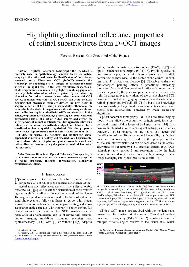
Optical coherence tomography (OCT) is a real time imaging modality that allows the acquisition of high-resolution cross-sectional images of thin layers of biological tissues [14]. It is now routinely used in ophthalmological settings, as it enables transverse optical imaging of the retina and hence the identification of the different neuronal layers (Fig. 1). Optical coherence tomography is based on the principle of the Michelson interferometer and can be considered as the optical equivalent of echography [15]. Spectral domain (SD) OCT technology now reaches 3 μm resolution while the high acquisition speed reduces motion artifacts, allowing reliable image averaging and good signal to noise ratio [16].

Fig. 1. OCT data acquired in a clinical setting [16] from a normal eye (on-axis image). Main retinal layers and interfaces: ILM – inner limiting membrane; RNFL – retinal nerve fiber layer; GCL – ganglion cell layer; IPL – inner plexiform layer; INL – inner nuclear layer; OPL – outer plexiform layer; HFL – Henle fiber layer; ONL – outer nuclear layer; IS – inner segments; OS – outer segments; IS/OS –inner segment/outer segment junction; COST – cone outer segment tips; RPE – retinal pigment epithelium; ChCap – chorio capillaris.

Clinical OCT images are acquired with the incident beam normal to the surface of the retina. Directional optical coherence tomography (D-OCT, Fig. 2) involves imaging at multiple off-axis angles relative to the visual axis, which

K. Grieve, M. Paques, Clinical Investigation Center 1423, Quinze-Vingts Hospital, 28 rue de Charenton, Paris, France.

Highlighting directional reflectance properties of retinal substructures from D-OCT images

Florence Rossant, Kate Grieve and Michel Paques

P

This is the author's version of an article that has been published in this journal. Changes were made to this version by the publisher prior to publication.The final version of record is available at http://dx.doi.org/10.1109/TBME.2019.2900425

Copyright (c) 2019 IEEE. Personal use is permitted. For any other purposes, permission must be obtained from the IEEE by emailing [email protected].

TBME-02046-2018

2

highlights the orientation of photoreceptor substructures and hence may detect misaligned photoreceptors. However, D-OCT is not yet available on standard OCT devices and custom OCT devices or specific protocols have to be designed along with image processing methods to analyse sets of images acquired at different angles.

Fig. 2. A set of D-OCT images acquired in a clinical setting from a normal eye. The yellow arrows show the direction of the incident light beam. The blue and red arrows point to areas of varying reflectance, in the Henle fiber layer (HFL).

Several research articles have already demonstrated the potential interest of D-OCT to highlight and analyse directional reflectance properties in the retina. Gao et al. first used a custom OCT setup to image off-axis macular photoreceptors and measure the contributions of macular photoreceptor substructures to the optical SCE (oSCE) [8]. They suggested that directional reflectance of the cone outer segment tip (COST) line and, to a lesser extent, of the inner/outer segment junction (IS/OS), accounts for most of the oSCE of macular photoreceptors. This was supported by the findings of Miloudi et al. who documented the directional reflectance of photoreceptors using a combined approach of en-face adaptive optics imaging and D-OCT [7].

The potential medical interest of D-OCT was highlighted by Lujan et al. who used D-OCT to delineate the Henle fiber layer, that is, the photoreceptor axons, and subsequently extract the thickness of the outer nuclear layer (ONL), which is an important biomarker of retinal degeneration [17]. Moreover, knowledge of the orientation of photoreceptors is essential because of the relationship between the direction of incident photons and the probability of their capture (and hence detection) by outer segments. The probability of capture is maximal when light is parallel to the physical orientation of the outer segment. This defines the Stiles-Crawford effect [1][2]. Hence, any change in the orientation of photoreceptors will decrease the efficiency of photon capture. Therefore, an automatic method to quantify the orientation of photoreceptors and disambiguate between loss and misorientation is of high interest for medical interpretation. Changes in photoreceptor anisotropy due to pathologies have been already observed using D-OCT in patients [18][19].

Nevertheless, few previous studies propose image processing solutions to finely highlight the directional reflectance

properties of photoreceptor substructures. In the literature, either standard commercial OCT devices [17][21][22] or custom multi-angle OCT devices [8][20] have been employed to acquire sets of multi-angle (directional) images. Custom OCT devices allow simultaneous acquisitions at several incidence angles, thus limiting aberrations due to the eye movement and allowing a better control of the incidence angles. In contrast, standard OCT devices are not designed for such use, and ad-hoc acquisition procedures are applied to sequentially acquire images at different angles, leading to higher variability in the set of multi-angle images (location of the slices, intensity distortions) and in the angles finally obtained. In all cases, image processing is limited in the literature to image registration, intensity normalization and color representation. An intensity normalization step is not always included in the processing algorithm, although it is a crucial issue. Indeed, there are possible variations of the measured signal due to optical properties of the tissues traversed (cornea, crystalline lens, nerve fiber layer), due to aberrations intrinsic to the eye and also due to the instrument (Fig. 3(a-c)), even in case of simultaneous acquisitions by a custom OCT apparatus [8]. So, without normalization, it is impossible to compare the intensity values across the stack of multi-angle images in a reliable and accurate way. Therefore, normalization is essential to highlight retinal structures showing directional reflectance properties and to estimate the relative amplitude of changes. In [8], each A-scan (i.e. each image column) is normalized to the same inner retinal reflection level, as the inner layers are assumed isotropic scatterers. In [20], data is normalized to the RPE layer, whose intensity is directionally invariant. Makhijani et al. rely on a region containing RPE and choroid to calculate a normalization function based on the measured mean and standard deviation; one function is calculated and applied per directional image [21]. These approaches all rely on a segmentation step to calculate the parameters of the normalization function(s), which may be complicated to achieve automatically in the case of diseased retinas where the retinal layers may be severely altered. Moreover, the processing is applied very locally without spatial regularization [8] or the same function is applied over the whole directional image [21], which does not deal with spatial variations of the overall image intensity. However, spatial variations of the signal intensity are obviously present in the directional images, especially when acquired with a standard commercial OCT device (Fig. 3(a-c)). Concerning colored representations of the directional reflectance properties, the common method is based on a chromatic visualization [17][20][21]. Given 3 directional images (one on-axis image and two off-axis images), each one is mapped to a color channel (red, green and blue) to generate the final color image. In this representation, isotropic pixels (i.e. with no significant intensity variation with respect to the angle) appear in gray levels, since the intensities are the same in the three color channels, while anisotropic pixels are attributed with a tint which reveals the angle of maximal intensity or a subset of dominant angles. The resulting colored images [17][20][21] may be challenging to interpret as the chromatic image is generally noisy and isotropic areas may be colored. This is probably because of the absence



TBME-02046-2018

3

or the weakness of the normalization step, as well as the lack of spatial regularization in the analysis of the angle-dependent intensity variations. Moreover, it is not possible to visualize the amplitude of the intensity variation with the angle.

In this article, we present advanced image processing methods to perform differential analysis of a set of D-OCT images and extract the angle-dependent retinal substructures. This work is an extension of our previous method [22] where we dealt with only 2 angles. We designed our algorithm to process directional images acquired with a standard SD-OCT device [16]. Our approach relies on a robust and accurate normalization algorithm, which includes two main steps: an individual correction applied to each directional image, to deal with inhomogeneous illumination over the image, and a joint illumination correction to normalize the directional images with respect to each other. Our algorithm does not need a prior segmentation of intra retinal layers or any assumption about isotropic areas. It only requires outlining of the whole retina (i.e. delineation of the inner limiting membrane (IML) and outer border of the retinal pigment epithelium (RPE), Fig. 5). Other strengths are the joint image processing and the possibility to estimate correction functions that spatially vary smoothly, allowing us to accurately compare pixel intensities. Finally, we also propose a robust color representation that facilitates interpretation of D-OCT data in general, by detecting and highlighting angle-dependent structures in healthy and diseased eyes. This colored representation is based on a pixel classification step followed by a Markovian regularization. It shows both the angle of maximal reflectance and the amplitude of the reflectance variation. Experimental results show evidence of photoreceptor disarray in a variety of retinal diseases, demonstrating the potential medical interest of the approach.

II. D-OCT

A. Subjects This was an observational, two center study. The study was

carried out according to the tenets of the Declaration of Helsinki and followed international ethical requirements. Informed consent was obtained from all patients. Eyes from 11 normal controls and eyes from 33 patients with various retinal diseases (macular edema, resolved macular edema, macular telangiectasia, acute macular neuropathy, serous detachment) were imaged during their routine follow-up. All eyes had a seemingly transparent ocular media.

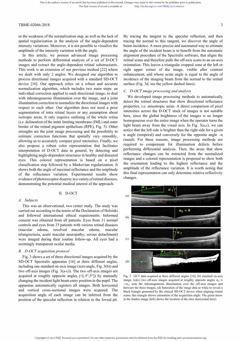
B. D-OCT acquisition protocol Fig. 3 shows a set of three directional images acquired by the

SD-OCT Spectralis apparatus [16] at three different angles, including one standard on-axis image (zero angle, Fig. 3(b)) and two off-axis images (Fig. 3(a-c)). The two off-axis images are acquired at roughly opposite angles (≈[-5°,5°]) by manually changing the incident light beam entry position in the pupil. The apparatus automatically registers all images. Both horizontal and vertical cross-sectional images were acquired. The acquisition angle of each image can be inferred from the position of the specular reflection in relation to the foveal pit.

By tracing the tangent to the specular reflection, and then tracing the normal to this tangent, we discover the angle of beam incidence. A more precise and automated way to estimate the angle of the incident beam is to benefit from the automatic alignment procedure of the Spectralis software, that aligns the retinal scans and therefore pulls the off-axis scans to an on-axis orientation. This leaves a triangular cropped zone at the left or right upper corner of the image, visible after contrast enhancement, and whose acute angle is equal to the angle of incidence of the imaging beam from the normal to the retinal surface (Fig. 3d, see the yellow dashed lines).

C. D-OCT image processing and analysis We developed image processing methods to automatically

detect the retinal structures that show directional reflectance properties, i.e. anisotropic areas. A direct comparison of pixel intensities across the D-OCT stack of images is not suitable here, since the global brightness of the images is no longer homogeneous over the entire image when the operator turns the light beam away from the visual axis. In Fig. 3(a,c), we can notice that the left side is brighter than the right side for a given α angle (temporal) and conversely for the opposite angle –α (nasal). For these reasons, image processing methods are required to compensate for illumination defects before performing differential analysis. Then, the areas that show reflectance changes can be extracted from the normalized images and a colored representation is proposed to show both the orientation leading to the highest reflectance and the amplitude of the reflectance variation. It is worth noting that this final representation can only determine relative reflectivity changes.

(a)

(b)

(c)

(d)

Fig. 3. OCT data acquired at three different angles [16]; (b) standard on-axis image, (a)(c) two off-axis images acquired at roughly opposite angles ≈− ; note the inhomogeneous illumination over the off-axis images and between the three images; (d) Saturation of the image data to white to reveal a black triangle generated by the clinical SD-OCT device when aligning retinal scans; this triangle allows estimation of the acquisition angle. The green arrow in the fundus image (left) shows the location of the slice (horizontal here).



TBME-02046-2018

4

The image processing methods (Fig. 4), developed in Matlab, are presented in Section III. They are based on three main steps: (i) a segmentation procedure to delineate the whole retinal area (Section III.A), (ii) a normalization algorithm to homogenize the intensities in the input images (Section III.B), (iii) a joint intensity analysis, including regularization procedures, to obtain a colored map showing the main anisotropic areas (Section III.C). The areas which have a peak of intensity in one of the three acquisition directions are represented by three colors, red, yellow and green for the negative, zero and positive angles respectively. The angle of each D-OCT acquisition is also estimated directly from the image itself (Section III.D). The quality of the results is assessed by checking that the RPE does not show directional reflectance in the final anisotropy map. The methods presented in Section III are an extension of our previous work [22]. The main improvements concern the method of joint illumination correction (Section III.B.2)), the estimation of the acquisition angle (Section III.D) and the differential analysis (Section III.C) which can now deal with three or more angles.

Fig. 4. Functional diagram of the proposed approach.

III. IMAGE PROCESSING METHODS Let us denote by ( , ) the standard on-axis OCT image

and by ( , ) and ( , ) the two off-axis images (Fig. 3(a-c)). The grayscale values are coded by floating point numbers in the interval [0,1]. The system of coordinates is defined by the origin at the upper left corner, the horizontal x axis and the vertical y axis (Fig. 5).

A. Preprocessing The delineation of the retina is necessary to determine the

area over which we have to correct the illumination. This is performed on the mean image that is calculated as the pixel-wise average of the input images. We apply the method of [23] to segment the inner limiting membrane (ILM) and the method of [24] to determine the outer edge of the retinal pigment epithelium (RPE) (Fig. 5). Horizontally, we restrict the region of interest (ROI) to the interval [ , ], 6mm wide, centered on the foveola

Fig. 5. Delineation of the region of interest (ROI).

These algorithms have proved to be robust even in cases of diseased retinas [23][24]. Contrary to [8][20][21], the complete delineation of the RPE and the segmentation of the inner layers (which are much more difficult to achieve) are not required.

B. Image normalization Image normalization aims to restore a homogeneous

brightness over the input images ( , ), ( , ) and ( , ) and normalize pixel intensities. This processing is necessary to compare the relative pixel intensities and detect anisotropic areas. We first propose an individual illumination correction, which is applied to each image separately. The underlying correction model is a linear function of the abscissa x, whose parameters are dynamically calculated from the image itself (Section III.B.1)). Then a joint optimization procedure is proposed to correct the two off-axis images and relative to the standard on-axis image , based on a polynomial regression applied iteratively (Section III.B.2)).

1) Individual illumination correction We first apply an illumination correction to the three images

separately to better balance their overall intensity. Let us denote the image to be processed by ( , ) (one of the three input images, , or , Fig. 6a). A classic background subtraction does not work on this type of image. Indeed, this type of correction assumes that the image is composed of small bright or dark objects over a homogeneous background. On the contrary, OCT images of the retina are made up of large stripes of different intensities. Therefore, our method relies on a model of intensity variation whose parameters are calculated from the image itself, considering its specific features. By observing the off-axis images, we note that the overall intensity mainly varies along the horizontal axis. So we propose to model the variation of the intensity ( ) as follows: ( , ) = ( )( , ) + ( )( , ) + (1)

In this equation, ( )( , ) represents the true value of

intensity of the pixel ( , ), i.e. the value we wish to recover, while ( , ) is the intensity measured in the source image; and are predefined positions (Fig. 6b). For pixels of abscissa

= , we have ( , ) = ( )( , ), i.e. no illumination distortion at the foveola. This model requires estimation of two parameters and . For that, we exploit the symmetry of the retinal layers with respect to the foveola to study the variation of intensity of the main clusters, as follows.

We divide the ROI of the input image ( , ) (Fig. 6a) into two sub-images (L) and (R), by slicing it vertically at the foveola . We classify the pixels of the retinal area into 3



TBME-02046-2018

5

classes with a K-means algorithm applied to both sub-images independently (Fig. 6b). We choose = 3 classes since three main reflectance levels are generally present in the OCT images, from very low levels (e.g. ONL, edema, etc.) to hyper reflective layers (e.g. RNFL, RPE, IS/OS) passing through intermediate values (e.g. OPL, GCL). Let us denote by ( ),

( ), k=1,2,3, the centers of the clusters (i.e. the mean intensity of the clusters) for the left (L) and right (R) sub-images. We use them to define three straight lines that each represent the variation of the actual value of the center of cluster k with respect to the x coordinate. The two points defining each of the three lines are set at about 2mm on either side of the foveola ( and x-coordinates), and take vertically the intensity value of the cluster ( ( ) and ( )) (Fig. 6b).

(a)

(b)

(c)

Fig. 6. Individual correction of the intensity of an input image; (b) k-means classification applied to input image (a), on the two half images separated at the foveola, and estimation of the intensity variation of the cluster centers; (c) corrected image.

The parameters a and b of (1) are estimated from points , ( ) and , ( ) , = 1,2,3. For each k, we assume that

( ) and ( ) are two distorted values of pixels of true intensity ( ) + ( ) 2⁄ , these pixels being respectively located at

and . This leads to a set of six equations (1), which can be reduced to a set of three linear equations (2).

( ) + ( ) + 2 = 2 ( ) − ( ) , = 1,2, … , 3 (2) Let us denote by and the least square solutions of (2).

We reverse equation (1) to get the transform to apply to each pixel ( , ) to correct its intensity ( , ):

( , ) = ( , ) − 1 + (3) We apply this processing to each input image separately and

we normalize the result in [0,1] by a linear contrast stretching. The corrected images are denoted by ′ , ′ and ′ . We can see

that the overall intensity of the off-axis images is better balanced after this correction (Fig. 6c, Fig. 8b). For the standard image , usually only contrast stretching is needed but we still apply the whole individual correction to deal with all cases and for the sake of homogeneity.

2) Joint illumination correction

The corrected images, denoted by ′ , = 1,2,3, are then jointly processed over the ROI. The standard on-axis image ′ is taken as reference and the two off-axis images ′ and ′ are corrected with respect to it. The idea is to minimize the number of pixels that differ in the reference image and in the processed off-axis image, assuming that most pixels of the ROI have the same reflectance whatever the light incidence.

We detail below the algorithm to process ′ . The same algorithm is applied to ′ . Our method relies on the approximation of the logarithm of the ratio of the two images (4) by a smooth surface.

( , ) = ln ( , )

( , ) (4)

( , ) is approximately equal to 0 for isotropic pixels, it is

positive or negative otherwise. The logarithmic scale is suitable here since inverse values for the ratio ( , ) ( , )⁄ are represented by opposite values of the same order of magnitude. To deal with noise, we approximate ( , ) by a polynomial function ( , ), whose order was empirically set to 3. Then, the off-axis image can be corrected as follows:

"( , ) = exp ( , ) ( , ) (5)

The coefficients of the polynomial function ( , ) are calculated by polynomial regression (least square minimization). It is important to fit the function only on pixels that are supposed to be isotropic (similar reflectance in ′ ( , ) and ′ ( , )). To do this, we calculate the histogram of over the ROI and we discard the % pixels that have the highest and lowest values. Moreover, we propose to apply this approach iteratively in order to refine the estimate of the correction function. The global algorithm is summarized below: Initialization: "( ) = Iterate: at iteration i

Calculate ( , ) = ln ( , )"( )( , )

Calculate the mask ℳ: discard p% pixels of the ROI, i.e. those with the lowest and highest values in .

Apply a polynomial regression to estimate the coefficients of the polynomial function ( )( , ) approximating ( , ) at pixels ( , ) ∈ ℳ.

Correct image: ∀( , ) ∈ , "( )( , ) = ( )( , ) "( )( , )

Until: max

( , )∈ℳ( )( , ) − min

( , )∈ℳ( )( , ) < and ≤ 25

The algorithm stops when the polynomial function is almost



TBME-02046-2018

6

flat, indicating that the pixels of the mask have similar values in images ′ ( , ) and "( ). The corrected image is the last

"( ) image, formally given by:

"( , ) = ( )( , ) ( , ) (6) with ( )( , ) = ∏ ( )( , )

The parameters are set to = 50% and = 10 . Fig. 7 shows the restoration functions ( ) and ( ) applied

respectively to ′ and ′ to get the normalized images " and " .

Fig. 7. Restoration functions ( ) (left) and ( ) (right). The function coefficients vary respectively in [0.8,1.1] and [0.8, 1.3].

(a) , , and

(b) , , and

(c) ", " , = " and "

Fig. 8. Main steps of the normalization algorithm: the three D-OCT images and the corresponding image of the standard deviation (7) calculated at each pixel; (a) input images; (b) after individual correction (Section III.B.1)); (c) after joint correction (Section III.B.2)).

Fig. 8 illustrates the main steps of the normalization algorithm: (a) the original images, (b) after the individual correction (Section III.B.1)) and (c) after the joint correction. At each step, the two first rows show the input or processed D-OCT images, and the third row shows the standard deviation calculated from the three images above:

( , ) = ∑ ( , ) − ∑ ( , ) (7) In (c), the anisotropic areas, including the Henle fiber and the

outer segments of the photoreceptors (Fig. 1), are highlighted in the standard deviation image, while isotropic areas appear now in black. The contrast between anisotropic and isotropic areas improves at each step of the normalization algorithm (see TABLE I in Section IV.B.2)). The individual correction step helps to homogenize the images and so to get a consistent mask in the first steps of the iterative joint correction algorithm. It is worth noting that the RPE is black in the final standard deviation image (c), which retrospectively validates our algorithm, as this layer is isotropic. In what follows, we will use the notation " = ′ to denote the normalized standard image.

C. Segmentation of the anisotropic areas and labelling 1) Classification and colored representation

We can now perform differential analysis on the normalized images. The aim is to classify the pixels into 4 classes. Class corresponds to pixels whose reflectance does not vary with the incidence of the light beam. Their value in the difference image

" = " − " (Fig. 9a) or in the standard deviation image " (Fig. 9b, (7)) is close to 0. Classes , and correspond respectively to pixels whose reflectance varies with the light angle, with a peak respectively in ", " or " .

(a)

(b)

(c)

(d)

Fig. 9. First classification in four classes. (a) difference image " = " − " , (b) standard deviation image " (7), (c) binary mask of anisotropic pixels, (d) resulting classification of the anisotropic pixels according to the angle leading to the maximal reflectance.

We first consider the images " and " , both normalized to 1, to detect the anisotropic pixels and calculate the mask (Fig. 9c). In theory, the difference image " reveals only pixels of classes 1 and 3. However, as it is of higher contrast than " , we rely on it to detect an initial set of anisotropic pixels, which are



TBME-02046-2018

7

then used to dynamically define the parameters of the processing to apply to " . Given a fixed threshold = 0.15 (experimentally tuned), we apply a hysteresis thresholding to " with low and high thresholds respectively set to and 2 . This gives an initial mask _ of anisotropic pixels. The mean and the standard deviation of the pixels of _ in " are calculated. We then apply a hysteresis thresholding to

" , with the high and low thresholds respectively set to and − . The resulting binary mask is denoted by (Fig. 9c).

Finally, we classify the anisotropic pixels with respect to the angle of maximal reflectance and so we get a first colored map

showing reflectance properties (Fig. 9d).

( , ) = ( , ) = 0

( , ) = 1 and arg max, ,

" ( , ) = (8)

2) Markovian regularization

The results presented in Fig. 9 can be regularized based on Markov random field (MRF) techniques [25], since the Markovian hypothesis allows us to take into account spatial interactions between connected pixels. We consider the K = 4 classes corresponding to the regions in black, green, yellow and red in (Fig. 9, equation (8)). Every pixel is characterized by the vector of its intensities in the three images ", i = 1,2,3:

( , ) =

"( , )"( , )"( , )

(9)

So we have a classification problem of dimension 3 with 4

classes. The initial classification enables us to estimate the probability density functions of intensities conditionally to the classes, denoted by ( ( , )| ( , ) = ). We assume that each one follows a Gaussian distribution. This assumption was verified experimentally on patches extracted from the images using the one-sample Kolmogorov-Smirnov test, with a 5% significance level. The parameters (mean vector) and Σ (covariance matrix) of the distributions are classically estimated from vectors belonging to class in the initial classification

(8). We refine this classification according to the Bayesian maximum a posteriori (MAP) criterion, i.e. by looking for the label configuration that maximizes the probability of the class field ( ( , )) conditionally to the observation field (the image data ( , )). This optimal configuration corresponds to a minimum state of an energy function U, defined as follows:

( | ) = ∑ ( , ) − ( , ) Σ ( , ) ( , ) −( , )

( , ) + ln (2 ) Σ ( , ) +

∑ φ ( , ), ( ′, ′)( , ),( , ) (10) where is the transpose of vector and ( ) the determinant of matrix . In this equation, ( , ) refers to the Potts model [26], expressing spatial dependencies between each

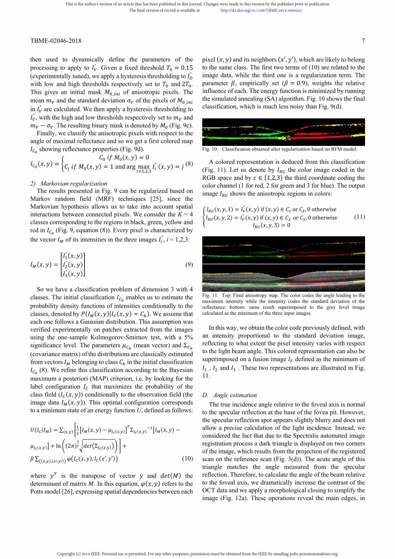
pixel ( , ) and its neighbors ( ′, ′), which are likely to belong to the same class. The first two terms of (10) are related to the image data, while the third one is a regularization term. The parameter , empirically set ( = 0.9), weights the relative influence of each. The energy function is minimized by running the simulated annealing (SA) algorithm. Fig. 10 shows the final classification, which is much less noisy than Fig. 9(d).

Fig. 10. Classification obtained after regularization based on RFM model.

A colored representation is deduced from this classification (Fig. 11). Let us denote by the color image coded in the RGB space and by ∈ {1,2,3} the third coordinate coding the color channel (1 for red, 2 for green and 3 for blue). The output image shows the anisotropic regions in colors:

( , , 1) = " ( , ) if ( , ) ∈ or , 0 otherwise( , , 2) = " ( , ) if ( , ) ∈ or , 0 otherwise

( , , 3) = 0 (11)

Fig. 11. Top: Final anisotropy map. The color codes the angle leading to the maximum intensity while the intensity codes the standard deviation of the reflectance; bottom: same result superimposed to the grey level image calculated as the minimum of the three input images.

In this way, we obtain the color code previously defined, with

an intensity proportional to the standard deviation image, reflecting to what extent the pixel intensity varies with respect to the light beam angle. This colored representation can also be superimposed on a fusion image defined as the minimum of

, and . These two representations are illustrated in Fig. 11.

D. Angle estimation The true incidence angle relative to the foveal axis is normal

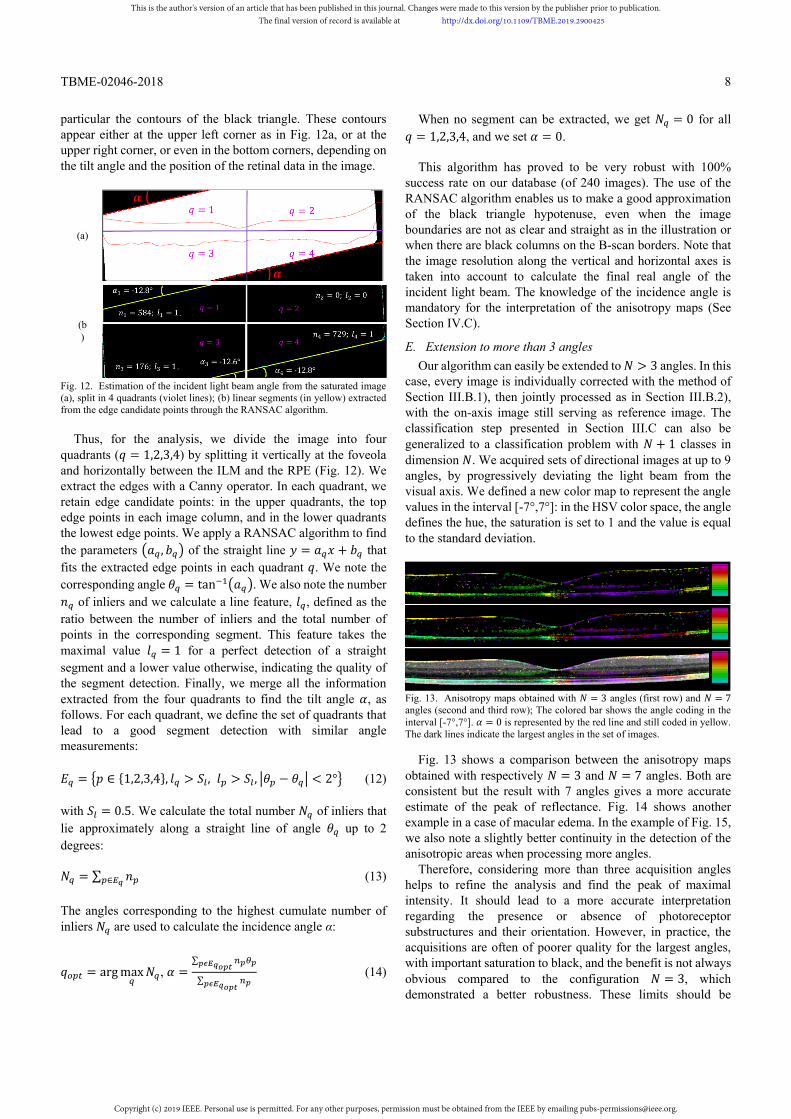
to the specular reflection at the base of the fovea pit. However, the specular reflection spot appears slightly blurry and does not allow a precise calculation of the light incidence. Instead, we considered the fact that due to the Spectralis automated image registration process a dark triangle is displayed on two corners of the image, which results from the projection of the registered scan on the reference scan (Fig. 3(d)). The acute angle of this triangle matches the angle measured from the specular reflection. Therefore, to calculate the angle of the beam relative to the foveal axis, we dramatically increase the contrast of the OCT data and we apply a morphological closing to simplify the image (Fig. 12a). These operations reveal the main edges, in



TBME-02046-2018

8

particular the contours of the black triangle. These contours appear either at the upper left corner as in Fig. 12a, or at the upper right corner, or even in the bottom corners, depending on the tilt angle and the position of the retinal data in the image.

(a)

(b)

Fig. 12. Estimation of the incident light beam angle from the saturated image (a), split in 4 quadrants (violet lines); (b) linear segments (in yellow) extracted from the edge candidate points through the RANSAC algorithm.

Thus, for the analysis, we divide the image into four

quadrants ( = 1,2,3,4) by splitting it vertically at the foveola and horizontally between the ILM and the RPE (Fig. 12). We extract the edges with a Canny operator. In each quadrant, we retain edge candidate points: in the upper quadrants, the top edge points in each image column, and in the lower quadrants the lowest edge points. We apply a RANSAC algorithm to find the parameters , of the straight line = + that fits the extracted edge points in each quadrant . We note the corresponding angle = tan . We also note the number

of inliers and we calculate a line feature, , defined as the ratio between the number of inliers and the total number of points in the corresponding segment. This feature takes the maximal value = 1 for a perfect detection of a straight segment and a lower value otherwise, indicating the quality of the segment detection. Finally, we merge all the information extracted from the four quadrants to find the tilt angle , as follows. For each quadrant, we define the set of quadrants that lead to a good segment detection with similar angle measurements:

= ∈ {1,2,3,4}, > , > , − < 2° (12)

with = 0.5. We calculate the total number of inliers that lie approximately along a straight line of angle up to 2 degrees:

= ∑ ∈ (13) The angles corresponding to the highest cumulate number of inliers are used to calculate the incidence angle α:

= arg max , =∑

∑ (14)

When no segment can be extracted, we get = 0 for all = 1,2,3,4, and we set = 0.

This algorithm has proved to be very robust with 100%

success rate on our database (of 240 images). The use of the RANSAC algorithm enables us to make a good approximation of the black triangle hypotenuse, even when the image boundaries are not as clear and straight as in the illustration or when there are black columns on the B-scan borders. Note that the image resolution along the vertical and horizontal axes is taken into account to calculate the final real angle of the incident light beam. The knowledge of the incidence angle is mandatory for the interpretation of the anisotropy maps (See Section IV.C).

E. Extension to more than 3 angles Our algorithm can easily be extended to > 3 angles. In this

case, every image is individually corrected with the method of Section III.B.1), then jointly processed as in Section III.B.2), with the on-axis image still serving as reference image. The classification step presented in Section III.C can also be generalized to a classification problem with + 1 classes in dimension . We acquired sets of directional images at up to 9 angles, by progressively deviating the light beam from the visual axis. We defined a new color map to represent the angle values in the interval [-7°,7°]: in the HSV color space, the angle defines the hue, the saturation is set to 1 and the value is equal to the standard deviation.

Fig. 13. Anisotropy maps obtained with = 3 angles (first row) and = 7 angles (second and third row); The colored bar shows the angle coding in the interval [-7°,7°]. = 0 is represented by the red line and still coded in yellow. The dark lines indicate the largest angles in the set of images.

Fig. 13 shows a comparison between the anisotropy maps obtained with respectively = 3 and = 7 angles. Both are consistent but the result with 7 angles gives a more accurate estimate of the peak of reflectance. Fig. 14 shows another example in a case of macular edema. In the example of Fig. 15, we also note a slightly better continuity in the detection of the anisotropic areas when processing more angles.

Therefore, considering more than three acquisition angles helps to refine the analysis and find the peak of maximal intensity. It should lead to a more accurate interpretation regarding the presence or absence of photoreceptor substructures and their orientation. However, in practice, the acquisitions are often of poorer quality for the largest angles, with important saturation to black, and the benefit is not always obvious compared to the configuration = 3, which demonstrated a better robustness. These limits should be



TBME-02046-2018

9

overcome when OCT technology integrates D-OCT functionality.

Fig. 14. Anisotropy maps obtained with = 3 angles (first row) and = 9 angles (second row) in case of macular edema. The detection of the peak of reflectance is more accurate with = 9.

Fig. 15. Anisotropy maps obtained with = 3 angles (first row) and = 9 angles (second row) in case of acute macular neuroretinopathy.

F. Summary We have presented in this section a complete algorithm to highlight and automatically extract the retinal structures which show variable reflectance properties. This method requires only the delineation of the whole retinal thickness and not the segmentation of individual retinal layers (Section III.A); The method first enhances the areas of anisotropy by compensating for illumination distortion (Section III.B), leading to a standard deviation image where the regions of variable reflectance are high contrast. The classification with Markovian regularization enables us to automatically extract these regions from the normalized D-OCT images and to label them according to the maximum reflectance angle (Section III.C). The corresponding incident angle is known accurately as it is calculated from the input images (Section III.D). The method can be extended to more D-OCT images and preliminary results are shown in Section III.E. The next section aims to present quantitative and qualitative results to demonstrate the improvements in comparison to previous algorithms [8][21][22] and to illustrate the medical interest.

IV. EXPERIMENTAL RESULTS We applied our algorithm on a database of 80 sets of D-OCT

images, acquired from 44 patients. Regarding pathologies, the database includes normal cases (37.5%), resolved macular edema (25%), macular edema (5%), macular telangiectasia (17.5%), acute macular neuropathy (2.5%), serous detachment (7.5%) and various other cases (5%). We checked for the presence of a specular reflection spot at the base of the foveal pit in each image to select acceptable sets of acquisitions.

A. Visual assessment The quality of the processing result was assessed by checking

that the RPE does not show directional reflectance in the final anisotropy map. An ophthalmologist also visually checked that the final anisotropy map is consistent with the observation of the input images. The new method of joint illumination correction has considerably improved the robustness of the algorithm, compared to [22] with now less than 10% failure. Overall, the final anisotropy maps are less noisy. They are also more accurate as we now deal with at least three angles instead of two. Cases of failure are mainly due to poor acquisition, i.e. a significant shift in the position of the slice between acquisitions, poor signal to noise ratio with bright speckles in at least one D-OCT image, or saturation of one off-axis image to white or black. The saturation to black or white results in loss of information and distorted correction functions ( )( , ) (6). Moreover, the new method of joint illumination correction (Section III.B.2)) and the angle calculus algorithm (Section III.D) have enabled us to extend our approach to more than three angles (Section III.E), demonstrating the possibility of accurately highlighting the orientation of photoreceptor substructures (Section IV.C).

B. Quantitative evaluation In this section, we provide quantitative results to demonstrate

the benefits of our normalization algorithm compared to previous ones [8][21][22]. We show how our method leads to a better contrast between isotropic and anisotropic areas and we evaluate the accuracy of the segmentation and classification of anisotropic structures.

1) Database for the quantitative evaluation

20 sets of D-OCT images are used for the quantitative evaluation. They were extracted from the complete database according to the following methodology: we first discarded sets of poor acquisitions,i.e. significant shift in the position of the slices (revealed by dissimilarities in the choroidal patterns) or very noisy images; then, we selected randomly 20 sets to encompass control cases (4 sets) and the various pathologies (16 sets). An ophthalmologist with 20-year’s experience in interpreting OCT images did manual segmentations, in order to delineate the inner layers (GCL+IPL+INL+OPL, denoted globally by IL in what follows), the retinal nerve fiber layer (RNFL), the Henle fiber layer (HFL), the COST line and the RPE (see Fig. 1). He also labelled the pixels of the COST line according to the classes defined in Section III.C.1). This work was done directly on the input D-OCT images, without any processing. Two other ophthalmologists did the same in order to study the inter-expert variability. These three experts are respectively denoted by Opht0, Opht1 and Opht2. 2) Contrast enhancement between isotropic and anisotropic areas

We analyze first the standard deviation image calculated from the D-OCT images (7) at different stages of the proposed normalization algorithm. Anisotropic layers such as the Henle fiber layer (HFL) and the COST line should be bright while isotropic layers such as the pigment epithelium (RPE), the inner layers (IL) and the retinal nerve fiber layer (RNFL) should be



TBME-02046-2018

10

dark. We estimate the mean power of the standard deviation image for a given region R by

( ) = 10 log

| |∑ ( , )( , )∈ (15)

The mean values obtained on the evaluation database are

indicated in TABLE I, with standard deviations: (a) before processing, (b) after the individual illumination correction (Section III.B.1)) and (c) after the complete normalization (Section III.B.2)). The overall contrast between isotropic and anisotropic structures is very low before any processing, with a mean power that may even be lower in the HFL than in the isotropic layers. The situation improves at each step of the method, with a final contrast of about 5-6 dB. This analysis shows that our normalization algorithm is efficient.

TABLE I

MEAN POWER (IN DB) OF RETINAL STRUCTURES IN THE STANDARD DEVIATION IMAGE AT DIFFERENT STAGES OF THE PROPOSED NORMALIZATION METHOD

(a) source images (b) after individual correction

(c) final normalization

( + ) −20.07 ± 2.20 −22.85 ± 0.92 −25.02 ± 1.22 ( ) −20.75 ± 2.61 −24.62 ± 1.62 −25.79 ± 1.19 ( ) −21.04 ± 2.31 −19.75 ± 2.32 −19.45 ± 2.62

3) Classification results We now evaluate our classification results (Section III.C) by

calculating sensitivity, precision and specificity indices. We first consider the isotropic vs. anisotropic binary classification. A true positive (TP) is a pixel belonging to an anisotropic region (HFL, COST line) which has been correctly classified as anisotropic (i.e. in class , or ) by our algorithm. A false negative (FN) is a pixel belonging to an anisotropic region (HFL, COST line) which has been set to class . A true negative TN (resp. false positive FP) is a pixel belonging to an isotropic region (RPE, IL, RNFL) classified in (resp. wrongly classified in , or ). Based on the manual segmentations, we calculate the sensitivity (true positive rate) and precision indices for the HFL and the COST line.

( ) = | |

| | | | (16)

( ) = | |

| | | | (17)

Note that isotropic pixels can be found on the COST line,

especially for pathological cases with damaged photoreceptors. Then we calculate the specificity (true negative rate) index for the isotropic regions (RPE, IL+RNFL):

( ) = | |

| | | | (18)

The closer these indices are to 1, the better the classification.

The ground truth is given by the manual segmentations and labelling of the most experienced ophthalmologist (Opht0). The averaged indices are reported in TABLE II.

TABLE II SENSITIVITY AND PRECISION INDICES FOR ANISOTROPIC RETINAL STRUCTURES

Auto/Opht0 Opht1/Opht0 Opht2/Opht0

HFL SENS 0.70 ± 0.16 0.82 ±0.10 0.84 ± 0.08 PREC 0.70 ± 0.11 0.73 ± 0.13 0.75 ± 0.11

COST line

SENS 0.88 ± 0.12 0.99 ± 0.02 0.87 ± 0.16 PREC 0.86 ± 0.17 0.84 ± 0.17 0.90 ± 0.12

TABLE III

CORRECT CLASSIFICATION RATE OF THE TP PIXELS OF THE COST LINE Auto/Opht0 Opht1/Opht0 Opht2/Opht0

CCR 0.66 ± 0.16 0.82 ± 0.16 0.77 ± 0.20

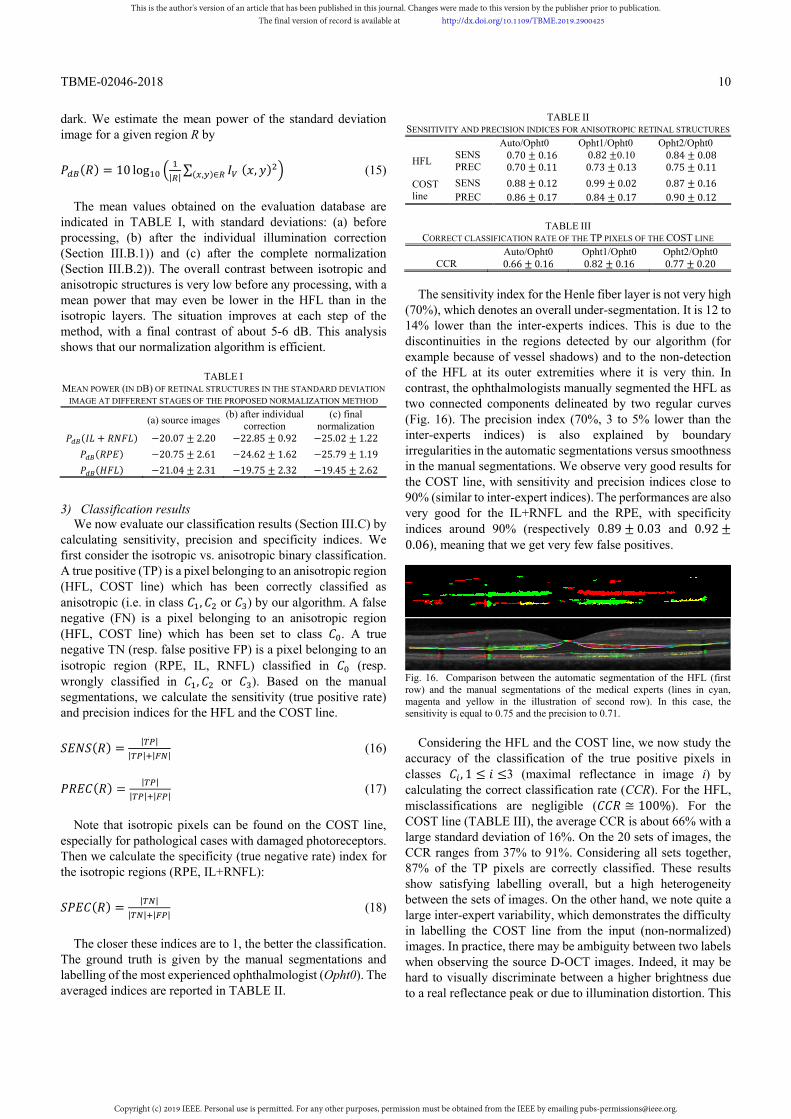
The sensitivity index for the Henle fiber layer is not very high (70%), which denotes an overall under-segmentation. It is 12 to 14% lower than the inter-experts indices. This is due to the discontinuities in the regions detected by our algorithm (for example because of vessel shadows) and to the non-detection of the HFL at its outer extremities where it is very thin. In contrast, the ophthalmologists manually segmented the HFL as two connected components delineated by two regular curves (Fig. 16). The precision index (70%, 3 to 5% lower than the inter-experts indices) is also explained by boundary irregularities in the automatic segmentations versus smoothness in the manual segmentations. We observe very good results for the COST line, with sensitivity and precision indices close to 90% (similar to inter-expert indices). The performances are also very good for the IL+RNFL and the RPE, with specificity indices around 90% (respectively 0.89 ± 0.03 and 0.92 ±0.06), meaning that we get very few false positives.

Fig. 16. Comparison between the automatic segmentation of the HFL (first row) and the manual segmentations of the medical experts (lines in cyan, magenta and yellow in the illustration of second row). In this case, the sensitivity is equal to 0.75 and the precision to 0.71.

Considering the HFL and the COST line, we now study the accuracy of the classification of the true positive pixels in classes , 1 ≤ ≤3 (maximal reflectance in image i) by calculating the correct classification rate (CCR). For the HFL, misclassifications are negligible ( ≅ 100%). For the COST line (TABLE III), the average CCR is about 66% with a large standard deviation of 16%. On the 20 sets of images, the CCR ranges from 37% to 91%. Considering all sets together, 87% of the TP pixels are correctly classified. These results show satisfying labelling overall, but a high heterogeneity between the sets of images. On the other hand, we note quite a large inter-expert variability, which demonstrates the difficulty in labelling the COST line from the input (non-normalized) images. In practice, there may be ambiguity between two labels when observing the source D-OCT images. Indeed, it may be hard to visually discriminate between a higher brightness due to a real reflectance peak or due to illumination distortion. This



TBME-02046-2018

11

ambiguity can only be solved by normalization. Since our normalization process leads to very consistent results on the HFL and RPE layers, as well as very consistent labels for normal COST lines, we can assume that our method actually solves this ambiguity and hence contributes to improved medical interpretation.

4) Comparison with other methods

We rely again on the analysis of the mean power of retinal layers in the standard deviation image (7)(15) to compare our normalization method with other described in the literature: our previous method [22], Gao’s method [8] and Makhijani’s algorithm [21]. Gao normalizes each A-scan to the same inner retinal reflection (i.e., the collective reflectance from the GCL, IPL, OPL and INL), which presumes prior segmentation of the RNFL/IPL+GCL interface and the OPL outer border (with the HFL). Makhijani detects the middle line of the RPE and calculates a normalizing function based on the mean and standard deviation in a region containing the RPE and the choroid. This process also relies on a segmentation step. In contrast, our previous algorithm [22] and the proposed method require only the delineation of the whole retina (i.e. ILM and RPE outer boundary, Fig. 5), which is not difficult to achieve automatically even for diseased eyes.

For a fair comparison, the mean power of the set of D-OCT images is adjusted to the same level over the ROI for the source images and the four evaluated methods. Thus, mean powers in the standard deviation images (7) can be compared directly.

TABLE IV

MEAN POWER (IN DB) OF RETINAL STRUCTURES IN THE STANDARD DEVIATION IMAGE FOR THE INPUT IMAGES AND AFTER NORMALIZATION

source Gao [8]

Makhijani [21]

Rossant [22] Our Method

(+ )

−20.07± 2.20

− .± .

−20.24± 1.94

−23.61± 1.10

−25.02± 1.22

( ) −20.75± 2.61

−18.62± 2.36

−22.07± 2.75

−24.22± 1.96

− .± .

( ) −21.04± 2.31

−20.38± 2.06

−21.14± 2.63

−19.67± 2.01

− .± .

All methods lead to a decrease of the mean power of isotropic

areas (IL+RNFL, RPE), with the exception of Gao’s, and an increase of the mean power of the anisotropic areas (HFL), with the exception of Makhijani’s. The best result for the IL+RNFL is achieved by Gao’s algorithm, which is not surprising as this algorithm normalizes the OCT data to the IL (segmented manually in this evaluation), however at the cost of poor performances on the RPE. Our method leads to the lowest power in the RPE and the highest in the HFL, to better balanced results for the isotropic regions, in a fully automated process. The quantitative results show also a significant improvement with respect to the previous method [22]: contrast between isotropic and anisotropic areas around 6 dB instead of 4 dB.

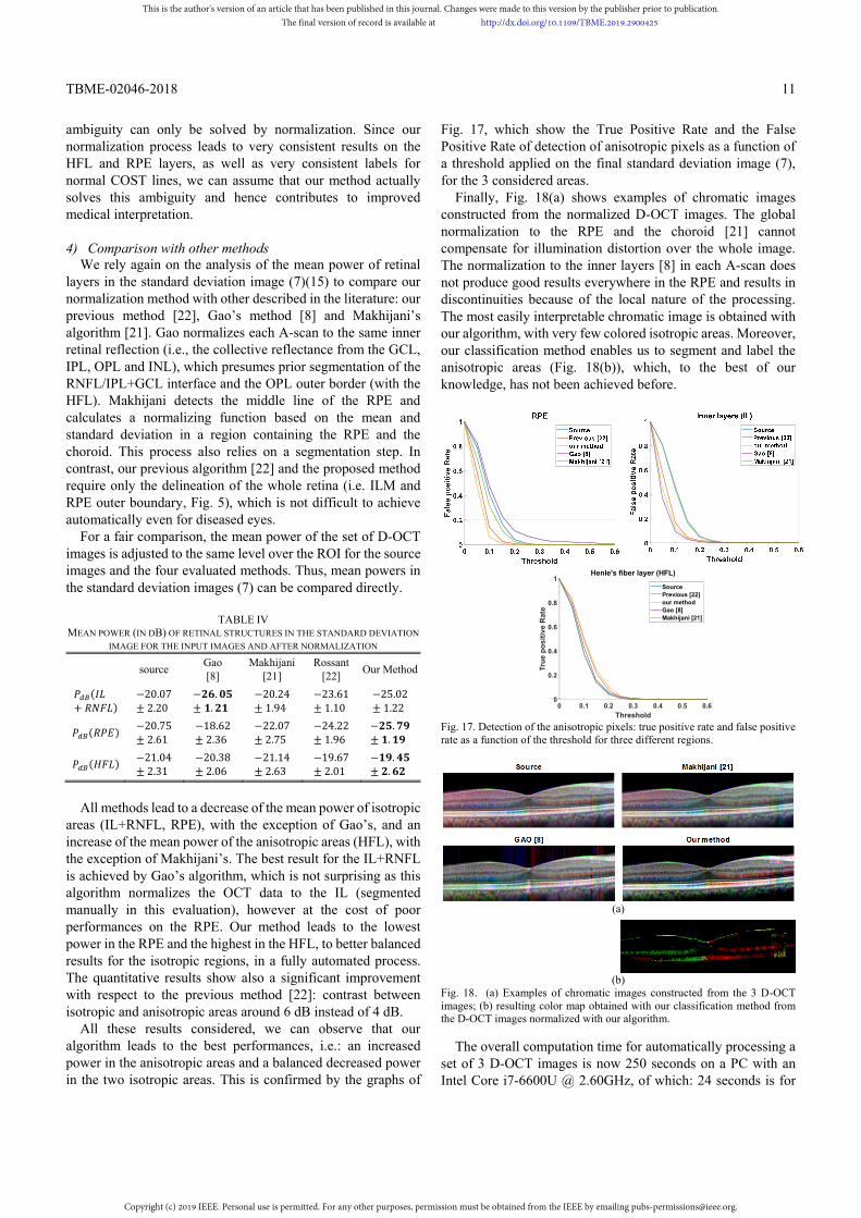
All these results considered, we can observe that our algorithm leads to the best performances, i.e.: an increased power in the anisotropic areas and a balanced decreased power in the two isotropic areas. This is confirmed by the graphs of

Fig. 17, which show the True Positive Rate and the False Positive Rate of detection of anisotropic pixels as a function of a threshold applied on the final standard deviation image (7), for the 3 considered areas.

Finally, Fig. 18(a) shows examples of chromatic images constructed from the normalized D-OCT images. The global normalization to the RPE and the choroid [21] cannot compensate for illumination distortion over the whole image. The normalization to the inner layers [8] in each A-scan does not produce good results everywhere in the RPE and results in discontinuities because of the local nature of the processing. The most easily interpretable chromatic image is obtained with our algorithm, with very few colored isotropic areas. Moreover, our classification method enables us to segment and label the anisotropic areas (Fig. 18(b)), which, to the best of our knowledge, has not been achieved before.

Fig. 17. Detection of the anisotropic pixels: true positive rate and false positive rate as a function of the threshold for three different regions.

(a)

(b)

Fig. 18. (a) Examples of chromatic images constructed from the 3 D-OCT images; (b) resulting color map obtained with our classification method from the D-OCT images normalized with our algorithm.

The overall computation time for automatically processing a set of 3 D-OCT images is now 250 seconds on a PC with an Intel Core i7-6600U @ 2.60GHz, of which: 24 seconds is for

0 0.1 0.2 0.3 0.4 0.5 0.6Threshold

0

0.2

0.4

0.6

0.8

1

True

pos

itive

Rat

e

Henle's fiber layer (HFL)

SourcePrevious [22]our methodGao [8]Makhijani [21]



TBME-02046-2018

12

the delineation of the region of interest (Section III.A), 25s for the normalization (Section III.B), 88 seconds for the classification (Section III.C) and 113 seconds for the estimation of the three incidence angles (Section III.D). The processing was 305 seconds long with our previous approach [22]. However, our software has not been optimized and we believe that the current overall computation time would be further reduced by using a C implementation.

C. Clinical interest Experimental results obtained from normal and pathological

cases are discussed below, demonstrating the potential of our image processing methods for clinical interpretation.

1) Normal cases

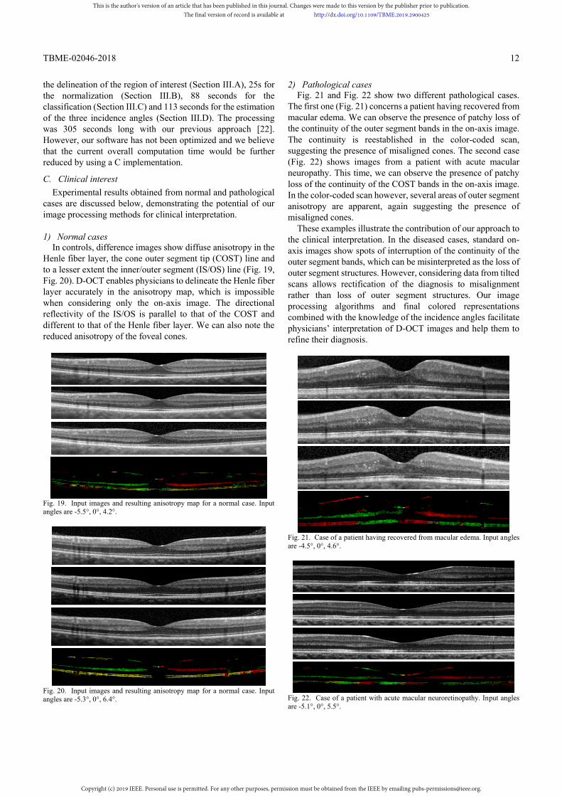
In controls, difference images show diffuse anisotropy in the Henle fiber layer, the cone outer segment tip (COST) line and to a lesser extent the inner/outer segment (IS/OS) line (Fig. 19, Fig. 20). D-OCT enables physicians to delineate the Henle fiber layer accurately in the anisotropy map, which is impossible when considering only the on-axis image. The directional reflectivity of the IS/OS is parallel to that of the COST and different to that of the Henle fiber layer. We can also note the reduced anisotropy of the foveal cones.

Fig. 19. Input images and resulting anisotropy map for a normal case. Input angles are -5.5°, 0°, 4.2°.

Fig. 20. Input images and resulting anisotropy map for a normal case. Input angles are -5.3°, 0°, 6.4°.

2) Pathological cases Fig. 21 and Fig. 22 show two different pathological cases.

The first one (Fig. 21) concerns a patient having recovered from macular edema. We can observe the presence of patchy loss of the continuity of the outer segment bands in the on-axis image. The continuity is reestablished in the color-coded scan, suggesting the presence of misaligned cones. The second case (Fig. 22) shows images from a patient with acute macular neuropathy. This time, we can observe the presence of patchy loss of the continuity of the COST bands in the on-axis image. In the color-coded scan however, several areas of outer segment anisotropy are apparent, again suggesting the presence of misaligned cones.

These examples illustrate the contribution of our approach to the clinical interpretation. In the diseased cases, standard on-axis images show spots of interruption of the continuity of the outer segment bands, which can be misinterpreted as the loss of outer segment structures. However, considering data from tilted scans allows rectification of the diagnosis to misalignment rather than loss of outer segment structures. Our image processing algorithms and final colored representations combined with the knowledge of the incidence angles facilitate physicians’ interpretation of D-OCT images and help them to refine their diagnosis.

Fig. 21. Case of a patient having recovered from macular edema. Input angles are -4.5°, 0°, 4.6°.

Fig. 22. Case of a patient with acute macular neuroretinopathy. Input angles are -5.1°, 0°, 5.5°.



TBME-02046-2018

13

Fig. 23 and Fig. 24 show other pathological examples. Good results are achieved despite the severe disorganization of the retinal layers. Indeed, our normalization and classification methods do not rely on a preliminary segmentation and manage to estimate the illumination distortion over the retina and compensate for it.

Fig. 23. Case of venous occlusion. Input angles are -6.3°, 1.5°, 3.4°

Fig. 24. Case of macular degeneration (macular telangiectasia). Input angles are -3.0°, 0°, 3.5°

Fig. 25. Case of serous retinal detachment. Input angles are -4.8°, -0.1°, 4.6°

Other cases of pathologies with even stronger disorganization have been successfully tested. For example, Fig. 25 shows a case of a serous retinal detachment. The color map is fully consistent with the observation of the source images. In a case with such major structural irregularities, the main difficulty lies in the manual acquisition of the slices at the exactly same location as the OCT apparatus has not been designed to make simultaneous acquisitions.

V. CONCLUSION AND PERSPECTIVES The potential medical interest of D-OCT, compared to

regular routine OCT, has been largely demonstrated in the literature. By acquiring a set of images at several angles of incidence, instead of only one in the direction of the optical axis, angle-dependent reflectance properties of photoreceptor substructures can be highlighted and studied. Thus, this technology adds a new dimension to the medical interpretation. However, few approaches have proposed image processing algorithms that enable effective detection and visualization of the angle-dependent reflectance areas, even when a dedicated D-OCT apparatus has been designed. The usually employed chromatic visualization is often very noisy with colored isotropic areas, and does not allow estimation of the extent to which the signal varies with the angle. In our view, the main issues are related to the normalization step, which is not accurate enough to allow a pixel-wise comparison of intensities across the stack of directional images. In this article, we have proposed an automatic algorithm to process D-OCT images acquired with a standard commercial OCT apparatus. This algorithm relies on a robust normalization algorithm that jointly processes the stack of images to homogenize the intensities. Contrary to previous methods, this algorithm relies on correction functions that vary smoothly over the image, so taking into account global illumination inhomogeneity. It also processes every off-axis image with respect to the standard on-axis image, leading to a better inter-image homogeneity. The differential analysis is done by a classification that is spatially regularized to enhance areas of anisotropy and reduce noise. The final anisotropy map shows both the angle of maximal reflectance, through a color code, and the amplitude of the signal variation, with an intensity proportional to the measured standard deviation. Experimental results have demonstrated the potential of this algorithm, which is fully automatic and can be extended to more than 3 directional images. The main limitations are due to the acquisition technology which does not allow accurate control of the acquisition angles and the location of the slices, and which can lead to very strong illumination distortions in the off-axis images (with saturation to black or white in some cases). We assume that our approach would lead to even more robust and accurate results were there a dedicated D-OCT acquisition technology to reduce these limiting factors. Given the importance of the information extracted from D-OCT, we should expect commercial adaptation of routine clinical OCT systems to include D-OCT functionality, in which case our image processing methods would become widely applicable in the ophthalmic imaging field.



TBME-02046-2018

14

ACKNOWLEDGMENT The authors would like to thank the medical team of the

Clinical Investigation Center of the Quinze-Vingts hospital for doing the manual segmentations that enabled us to evaluate our image processing methods.

REFERENCES [1] W. Stiles, “The luminous efficiency of rays entering the eye pupil at different

points,” Proceedings of the Royal Society of London B: Biological Sciences 112(778), pp. 428–450, 1933.

[2] G. Westheimer, “Directional sensitivity of the retina: 75 years of stilesCcrawford effect,” Proceedings of the Royal Society of London B: Biological Sciences 275(1653), pp. 2777–2786, 2008.

[3] A. Roorda, D. R. Williams, “Optical fiber properties of individual human cones,” Journal of Vision 2(5), pp. 4-4, 2002.

[4] P.J. Delint, T.T.J.M. Berendschot, D. van Norren, “Local photoreceptor alignment measured with a scanning laser ophthalmoscope,” Vision Research 37(2), pp. 243–248, 1997.

[5] D. Rativa, B. Vohnsen, “Analysis of individual cone-photoreceptor directionality using scanning laser ophthalmoscopy,” Biomedical Optics Express 2(6), pp. 1423–1431, 2011.

[6] H.J. Morris, L. Blanco, J.L. Codona, S.L. Li, S.S. Choi, N. Doble, “Directionality of individual cone photoreceptors in the parafoveal region,” Vision Research 117, pp. 67–80, 2015.

[7] C. Miloudi, F. Rossant, I. Bloch, C. Chaumette, A. Leseigneur, J.-A. Sahel, S. Meimon, S. Mrejen, M. Paques, “The negative cone mosaic: A new manifestation of the optical stiles-crawford effect in normal eyes,” Investigative Ophthalmology & Visual Science 56(12) 7043–7050, 2015.

[8] W. Gao, B. Cense, Y. Zhang, R. S. Jonnal, D. T. Miller, “Measuring retinal contributions to the optical stiles-crawford effect with optical coherence tomography,” Optics Express 16 (9), pp. 6486–6501, 2008.

[9] S. S. Choi, L. F. Garner, J. M. Enoch, “The relationship between the stiles-crawford effect of the first kind (SCE-I) and myopia,” Ophthalmic and Physiological Optics 23(5), pp. 465–472, 2003.

[10] H. E. Bedell, J. M. Enoch, C. R. Fitzgerald, “Photoreceptor orientation: A graded disturbance bordering a region of choroidal atrophy,” Archives of Ophthalmology 99(10), pp. 1841–1844, 1981.

[11] D. G. Birch, M. A. Sandberg, E. L. Berson, “The stiles-crawford effect in retinitis pigmentosa,” Investigative ophthalmology & visual science 22(2) pp. 157–164, 1982.

[12] C. W. Lardenoye, K. Probst, P. J. DeLint, A. Rothova, “Photoreceptor function in eyes with macular edema,” Investigative ophthalmology & visual science 41(12) pp. 4048–4053, 2000.

[13] M. J. Kanis, R. P. Wisse, T. T. Berendschot, J. van de Kraats, D. van Norren, “Foveal cone-photoreceptor integrity in aging macula disorder,” Investigative ophthalmology & visual science 49(5), pp. 2077– 2081, 2008.

[14] D. F. Kiernan, W.F. Mieler, S.M. Hariprasad, “Spectral-domain optical coherence tomography: a comparison of modern high-resolution retinal imaging systems,” American journal of Ophthalmology 149(1) pp. 18–31, 2010.

[15] M. Born, E. Wolf, “Interference and diffraction with partially coherent light,” Principles of optics, 6(1), pp. 491–555, 1993.

[16] Heidelberg engineering; https://business-lounge.heidelbergengineering.com/fr/en/products/spectralis/

[17] B. J. Lujan, A. Roorda, J. A. Croskrey, A. M. Dubis, R. F. Cooper, J.-K. Bayabo, J. L. Duncan, B. J. Antony, J. Carroll, “Directional optical coherence tomography provides accurate outer nuclear layer and henle fiber layer measurements,” Retina (Philadelphia, Pa.) 35(8), pp. 1511, 2015.

[18] B. J Lujan, E. Y Chew, J. L Duncan, B. J Antony, V. Makhijani, A. Roorda; Altered Photoreceptor Bands Surrounding Areas of Loss in MacTel Cause En Face OCT Endpoint Variability. Invest. Ophthalmol. Vis. Sci. 2016;57(12):4250

[19] A. Pedinielli, M. Lagarrigue, S. Mrejen, F. Rossant, R. Tadayoni, A. Gaudric, V. Krivosic, M. Paques, Photoreceptor anisotropy in macular oedema and MacTel: a multiangle OCT study. Invest. Ophthalmol. Vis. Sci. 2016;57(12):4248

[20] A. Wartak, M. Augustin, R. Haindl, F. Beer, M. Salas, M. Laslandes, C. K Hitzenberger, “Multi-directional optical coherence tomography for retinal imaging,” Biomedical optics express, 8(12), pp. 5560-5578, 2017.

[21] V. S. Makhijani, A. Roorda, J. K. Bayabo, K. K. Tong, C. A. Rivera-Carpio, B. J. Lujan, “Chromatic visualization of reflectivity variance within hybridized directional oct images,” Optical Coherence Tomography and Coherence Domain Optical Methods in Biomedicine XVII, Vol. 8571, p. 857105, 2013.

[22] F. Rossant, K. Grieve, M. Paques, “Automated analysis of directional optical coherence tomography images,” in Proc. International Conference Image Analysis and Recognition, Montreal, 2017, pp. 524–532.

[23] I. Ghorbel, F. Rossant, I. Bloch, S. Tick and M. Paques, “Automated segmentation of macular layers in OCT images and quantitative evaluation of performances,” Pattern Recognition, 44(8), pp. 1590-1603, 2011.

[24] F. Rossant, I. Bloch, I. Ghorbel, and M. Pâques, “Parallel Double Snakes. Application to the segmentation of retinal layers in 2D-OCT for pathological subjects,” Pattern Recognition, 48(12), pp. 3857-3870, 2015.

[25] Geman, S. Geman, D., “Stochastic relaxation, Gibbs distribution, and the Bayesian restoration of images,” IEEE Transaction on Pattern Analysis and Machine Intelligence 6(6), pp. 721–741, 1984.

[26] J. Besag, “On the statistical analysis of dirty pictures,” Journal of the Royal Statistical Society, Series B-48 pp. 259–302, 1986.



highlighting directional reflectance properties of retinal

Documents