highlighting the history of japanese radio

Journal of Astronomical History and Heritage, 18(3), 285–311 (2015).

Page 285

THE HISTORY OF EARLY LOW FREQUENCY RADIO ASTRONOMY IN AUSTRALIA. 4: KERR, SHAIN,

HIGGINS AND THE HORNSBY VALLEY FIELD STATION NEAR SYDNEY

Wayne Orchiston

National Astronomical Research Institute of Thailand, 191 Huay Kaew Road, Suthep District, Muang, Chiang Mai 50200, Thailand, and University of

Southern Queensland, Toowoomba, Queensland, Australia. Email: [email protected]

Bruce Slee CSIRO Astronomy and Space Sciences, Sydney, Australia.

Email: [email protected]

Martin George

National Astronomical Research Institute of Thailand, 191 Huay Kaew Road, Suthep District, Muang, Chiang Mai 50200, Thailand, and University of

Southern Queensland, Toowoomba, Queensland, Australia. Email: [email protected]

and

Richard Wielebinski Max-Planck-Institut fur Radioastronomie, Bonn, Germany, and University

of Southern Queensland, Toowoomba, Queensland, Australia. Email: [email protected]

Abstract: Between 1949 and 1952 the CSIR‘s Division of Radiophysics was a world leader in low frequency radio

astronomy, through research conducted mainly by Alex Shain and Charlie Higgins at their Hornsby Valley field station near Sydney. In this paper we discuss the personnel, radio telescopes and research programs (mainly conducted at 9.15 and 18.3 MHz) associated with the Hornsby Valley site.

Keywords: Australian low frequency radio astronomy, CSIRO Division of Radiophysics, Hornsby Valley field station,

Alex Shain, Charlie Higgins, Frank Kerr.

1 INTRODUCTION

As documented elsewhere (see Orchiston et al., 2015; 2016; George et al., 2015a) Australia was an early international leader in low frequency radio astronomy, with two centres of excellence. One was near Sydney, and the other was in the island state of Tasmania to the south of the Australian mainland.

The Sydney initiatives were under the au-spices of the CSIRO‘s Division of Radiophysics (henceforth RP),

1 which from 1946 through into

the early 1960s maintained a large number of field stations and remote sites, mainly in and around Sydney (Orchiston and Slee, 2005a; Rob-ertson, 1992; Sullivan, 1988). Their distribution is shown in Figure 1. Two of these field stations, Hornsby Valley (Orchiston and Slee, 2005b) and Fleurs (Orchiston and Slee, 2002), were involved in low frequency radio astronomy—that is, re-search conducted at frequencies below 30 MHz.

This paper details the pioneering low frequen-cy radio astronomy that was carried out at the Hornsby Valley field station between 1946 and 1952.

2

Figure 1: A map showing the field stations and remote sites, mainly in the Sydney region, maintained by the CSIRO‘s Division of Radiophysics between 1946 and 1965. Hornsby Valley is Site 9. The approximate present-day boundary of suburban Sydney is indicated by the upper dotted line.

mailto:[email protected]

mailto:[email protected]

mailto:r.wielebinski@xxx

W. Orchiston, B. Slee, M. George and R. Wielebinski Early Low Frequency Radio Astronomy in Australia: 4

86

Figure 2: A view across Old Man Valley towards the distant farm house on the hillside, and showing the collection of ex-WWII buildings associated with the field station‘s early research programs (courtesy: CSIRO RAIA B1266-15).

Figure 3: A close-up of the assemblage of huts, trailers, poles and wiring associated with the Moon bounce experiment (courtesy: CSIRO RAIA B1266-5).

W. Orchiston, B. Slee, M. George and R. Wielebinski Early Low Frequency Radio Astronomy in Australia: 4

Page 287

2 THE HORNSBY VALLEY FIELD STATION

2.1 Introduction3

The Hornsby Valley field station (Orchiston and Slee, 2005b), site 9 in Figure 1, was established in 1946 on farmland in a picturesque valley surrounded by low tree-covered hills (see Figure 2).

4 Locally, this radio-quiet location was refer-

red to as ‗Old Man Valley‘, and at the time it lay just beyond Sydney‘s most northerly suburbs.

From the start, the field station featured a centralised cluster of ex-WWII portable huts and mobile trailers that were used to house the scientific equipment. These are shown in close up in Figure 3.

The first scientists to carry out research at this new field station were Frank Kerr and Alex Shain. Frank John Kerr (1918–2000; Figure 4) was born in St Albans while his Australian parents temporarily were in England. After graduating with B.Sc. and M.Sc. degrees in physics from the University of Melbourne he joined RP in 1940. There he was involved in a range of radar research and followed up by carrying out radar research at the Hornsby Valley field station immediately after WWII. In 1948 he transferred to the Potts Hill field station (site 16 in Figure 1) and later became an authority on H-line emission (see Kerr, 1984; Wendt et al., 2011). He went to the USA in 1951, where he built up his astronomical know-ledge and expertise by completing a Masters in Astronomy at Harvard University. After return-ing to RP and beginning H-line research, Kerr later followed a pattern established in 1955 by his distinguished RP colleague, Ronald Newbold Bracewell (1921–2007; Thompson and Frater, 2010), and accepted a Chair in Astronomy at the University of Maryland in 1966. He remain-ed in the USA until his death in 2000 (Wester-hout, 2000).

Charles Alexander (‗Alex‘) Shain (1922–1960; Figure 5) was born in Melbourne, and after com-pleting a B.Sc. at the University of Melbourne and serving briefly in the military he joined the CSIR‘s Division of Radiophysics in November 1943 (Orchiston and Slee, 2005b). He assisted in the development of radar during WWII, and from late 1946 he was one of those scientists charged with identifying peace-time research that would take advantage of the war-time tech-nological achievements of the Division. It is im-portant to remember that at this time

Radiophysics was CSIR‘s glamour division, arguably containing within its walls the densest concentration of [radar-related] technical talent on the continent ... (Sullivan, 2009: 122).

Shain was among a coterie of young re-searchers who would quickly make Australia a world leader in the emerging field of radio astron-

Figure 4: Frank Kerr in 1952 (cropped close-up taken from CSIRO RAIA B2842-45).

omy,5

and he pioneered research at low fre-quencies. Unfortunately, Shain‘s inspiring lead in this field was cut short prematurely when he succumbed to terminal cancer on 11 February 1960, just five days after his 38th birthday. This was a tragic loss for Australian and international radio astronomy, as documented by Dr Joseph Lade (‗Joe‘) Pawsey (1908–1962), the Deputy Chief of the Division of Radiophysics, who des-cribed Alex Shain as ―... a wonderful colleague in the laboratory, imaginative, well balanced, ex-ceedingly unselfish, and a real friend to all.‖ (Paw-sey, 1960: 245).

Aiding Kerr and Shain at Hornsby Valley was Technical Assistant Charles S. (‗Charlie‘) Higgins (Figure 6), who came to Radiophysics from a radio company. He had a certificate in radio en-gineering and an interest in astronomy.

2.2 The Moon-Bounce Experiment

It is interesting that the first scientific research conducted at Hornsby Valley field station had nothing to do with radio astronomy, or astron-omy. Rather it focussed on radar astronomy, and was motivated by ionospheric research.

It was natural that this research should be led by Frank Kerr, who wished to use Moon-bounce experiments to investigate the ionosphere. But while he and Alex Shain were the first Austra- lians to employ radar astronomy in this way, they

Figure 5 (left): Alex Shain in 1952 (cropped close-up taken from CSIRO RAIA B2842-133). Figure 6 (right): Charlie Higgins in 1952 (cropped close-up taken from CSIRO RAIA B2842-132).

W. Orchiston, B. Slee, M. George, and R. Wielebinski Early Low Frequency Radio Astronomy in Australia: 4

Page 288

were not the first to attempt radar astronomy. As Sullivan (2009) has documented, in 1940 Kerr and Shain‘s RP colleague, Jack Hobart Pid-dington (1910–1997), produced a 3-page report that included the following perceptive com-ments:

With the enormous powers available from R.D.F. [radio direction finding; i.e. radar] equip-ment, the possibility of obtaining echoes from the Moon appears worthy of investigation. (Pid-dington, 1940).

Figure 7: Two different views of some of the equipment used by Kerr and Shain for their 1947 Moon-bounce experiment (courtesy: CSIRO RAIA B1266-14 and B1266-21).

However, Brown (1999) reveals that it was two German radar experts, Wilhelm Stepp and Willi Thiel, who in the winter of 1943–1944 bounced radar signals off the Moon using an experiment-al radar set near Göhren on the island of Rügen, about 200 km northeast of Hamburg.

The first published accounts of successful Moon-bounce experiments occurred in early 1946 when an American team led by John Hib-

bert DeWitt (1906–1999) carried out ‗Project Diana‘ (see Clark, 1980), and Zoltán Bay (1900– 1992; Wagner, 1985) and his collaborators also had success in war-torn Hungary (see Bay, 1946). In the extensive report on their investiga-tions at 111.5 MHz, DeWitt and Stodola (1949) noted that the received signal, which should have been 100 times greater than the receiver noise level, only occasionally reached this figure but usually showed severe fading and some-times could not be detected at all! Pawsey and Bracewell (1955: 294; our italics) remark that

This low signal and its occasional disappear-ance is a remarkable result … The only known factor is the obstruction offered by the iono-sphere … There is either some important un-known factor influencing transmission between us and the moon or reflection from the moon, or the Signal Corps’ observations were at fault. The data given do not permit us to exclude the latter possibility.

It was against this background that Kerr and Shain planned their own Moon-bounce experi-ment, but whereas the deWitt and Bay projects were undertaken as technical challenges the Hornsby Valley project had clear scientific objec-tives. Thus, Kerr and Shain wanted to know

… why the echoes recorded by DeWitt‘s team had behaved so erratically .... This, they thought, might well be an ionospheric effect, or even caused in interplanetary space by streams of charged particles shot from the sun. (Sul-livan, 2009: 274).

Their Hornsby Valley experiment was carried out during 1947–1948, and in the opinion of Pawsey and Bracewell (1955: 294) was

... a very neat arrangement. Instead of build-ing special transmitting equipment they utilized an existing short-wave 100-kilowatt transmit-ter, Radio Australia, and an aerial system nor-mally used to broadcast to North America. (ibid.).

This was a rhombic aerial, attached to a receiv-er that was tuned to receive 17.84 and 21.54 MHz signals broadcast by Radio Australia from Shepparton, Victoria (~600 km south of Hornsby Valley). The transmissions were triggered by Kerr and Shain using a landline connection, and when the Moon rose through the beam of the rhombic aerial they searched for echoes that exhibited the expected 2.5-second delay. Fig-ure 7 shows some of the equipment used in this experiment. The receiver was an

R.C.A. type AR88 communication receiver,

with the band-width adjusted to 70 c/s. The stability with regulated [power] supplies was such that slight retuning was necessary every 10–15 minutes … [while the display comprised a] (a) Long-persistence cathode-ray tube, and photographic recording … [and] (b) Loud-speaker, using the beat-frequency oscillator of the receiver. The aural method was the more


Page 289

sensitive for the detection of weak signals. (Kerr et al., 1949: 310).

The times when observations could be made were limited to two periods of several succes-sive days each month when the Moon passed through the beam of the rhombic aerial, and only when Radio Australia was not broadcasting, i.e. between 0230 and 0530 and from 0930 to 1230 Eastern Australian Standard Time. However, be-cause of atmospherics, observations normally were restricted to the first of these intervals.

For this experiment three different types of signals were broadcast:

(a) A group of three ¼-second pulses (used in searching for echoes and for identification of weak echoes). (b) A single pulse 2.2 seconds long (for studying short-period amplitude variations of the echo). (c) A group of pulses of length 1 millisecond and recurrence frequency 40 cps, extending over a total period of 2.2 seconds (for exam-ining the fine structure of the echo) …

The pulse group repetition period was 6 seconds in all cases. (Kerr and Shain, 1951: 230–231).

From July 1947 Moon-bounce transmissions were made on every possible occasion over a period of slightly longer than one year. In all, 28 experiments were carried out at Hornsby Valley and echoes were received on 22 of these. Fig-ures 8 and 9 are included here to show the types of results obtained. The first of these shows the use of three short pulses, received directly from Shepparton via E-region scatter (the direct signals), followed ~2.5 seconds later by three echo pulses from the Moon, which are ―… generally unequal in amplitude.‖ (Kerr and Shain, 1951: 232). By way of contrast, Figure 9 shows

… a series of three successive signals of the long pulse type (only the first of these is labelled in the figure). By this method a record of echo intensity is obtained over a series of

Figure 8: An example of a photographic record showing the results obtained from using a group of three short pulses (after Kerr and Shain, 1951: 232).

2.2-second periods interrupted by breaks 3.8 seconds long. (ibid.).

Through this research, Kerr and Shain were able to show that

… the reduced echo intensity … was connect-ed with obstruction in the F2 region of the ionosphere, though it could not be accounted for on current models. Their investigations therefore led fundamentally to a geophysical discovery … [and] showed there are gaps in our knowledge of the ionosphere. (Pawsey and Bracewell, 1955: 294–295; our italics).

However, what particularly interests us here is the astronomical conclusion that Kerr and Shain (1951: 230; our italics) were able to draw on the basis of their observations:

The received echoes showed two types of fad-ing. One type was consistent with an iono-spheric origin. The second has been shown to be due to the moon‘s libration, effective re-flection taking place over a large proportion of the moon‘s surface. This, together with the elongation of short pulses on reflection, demon-strates that the moon is a “rough” reflector …

This project was Frank Kerr‘s sole post-war exploration at low frequencies.

Figure 9: A photographic record showing three successive Moon-bounce echoes obtained with 2.2 second signals. These echoes show rapid fading caused by the F- layer, while the small fluctuations present are due to cosmic noise (after Kerr and Shain, 1951: 232).


Page 290

Figure 10: Plan of the dipole array (after Shain, 1951: 259).

2.3 The 18.3 MHz Galactic Survey

In mid-1948 at the end of the Moon-bounce experiment Kerr moved to the Potts Hill field station, leaving the Hornsby Valley in the cap-able hands of Alex Shain and Charlie Higgins. They and Dr Joe Pawsey had decided to chart a new course for RP by developing Hornsby Valley as the Division‘s forefront low frequency radio astronomical facility.

In deciding to conduct their first experiments at 18.3 MHz, Shain (1951: 258) perceptively pointed out that previously Figure 11: A corrected plot of equivalent aerial temperature versus sidereal time (after Shain, 1951: 264).

Figure 12: Equivalent aerial temperature versus sidereal time at 18.3 MHz (a) and 100 MHz (b and c) (after Shain, 1951: 265).

The most useful series of observations … [at about this frequency] has been the early work of Jansky (1937) on frequencies near 20 Mc/s.

Jansky was, of course, the founder of radio astronomy, and it is telling that Shain and Hig-gins were the first to carry out serious low fre-quency observations since the 1930s.

Their equipment comprised

… an array of eight half-wave dipoles connect-ed in phase, supported 0.2 wavelengths above ground, and arranged in plan … [as shown here in Figure 10, and connected to a] stan-dard communications receiver with a band-width of 400 c/s. … The output was indicated by a milliameter with D.C. amplifier connected to the second detector. (Shain, 1951: 259).

Observations were carried out between May and November 1949. Because the latitude of the Hornsby Valley site was 34° S and

… the direction of maximum sensitivity of the aerial was fixed vertically upwards .... [the] observations therefore give a weighted aver-age of the radio emission from a zone of sky about Declination –34°. This zone includes both the centre and south pole of the Galaxy. (Shain, 1951: 258).

After allowing for ionospheric effects, a plot of equivalent aerial temperature versus sidereal time was prepared (Figure 11), which clearly showed the anticipated maximal emission along the plane of our Galaxy.

However, Shain (1951: 264) noted that

Because the observations were limited to a fixed aerial direction, and since the aerial has an angular beam width comparable to the dimensions of certain features of the galactic noise distribution, the result of the observa-tions … gives only a rough indication of the noise distribution across the sky.

Shain then used the 100 MHz contour diagram obtained by Bolton and Westfold (1950) to cal-culate the equivalent aerial temperatures at this frequency, and compared the corrected results with his 18.3 MHz plot (see Figure 12). He found that

… although the shape of the two curves is roughly similar, the observed ratio of maximum to minimum is considerably lower than that expected from 100 Mc/s. results … [Nonethe-less] a good fit could be obtained using the relation

T18.3 = 200,000(1 – e– T100/1900

) °K. [sic],

where T18.3 is the temperature to be attached to the contour corresponding to T100 in the 100 Mc/s. survey. (Shain, 1951: 264–265).

However, it is not a perfect fit, as there are not-able differences between curves (a) and (c) in Figure 12 at sidereal times 11–15 hours and 19–22 hours. Shain (1951: 266) suggests that ―One possible explanation of at least part of the

http://articles.adsabs.harvard.edu/cgi-bin/nph-iarticle_query?bibcode=1951AuSRA...4..258S&db_key=AST&page_ind=1&data_type=GIF&type=SCREEN_VIEW&classic=YES


Page 291

discrepancy is the effects of radiation from

discrete sources of noise.‖ One of these is the strong source Centaurus A. Allowing for these discrete sources, Shain then converted his 18.3 MHz diagram into an isophote plot, and this is shown in Figure 13.

Shain (1951: 267) concludes this pioneering paper:

These observations confirm that the intensity of galactic radiation at 18.3 Mc/s. is high and of the order of magnitude suggested by the observations of Jansky ...

The observations indicate anomalies in the attenuation of radio waves penetrating the ion-osphere, F-region attenuation being higher and lower-layer attenuation being lower than expected …

The observations are reasonably consist-ent with the hypothesis that contours of equal intensity of galactic radiation have the same shape at 18.3 Mc/s. as at 100 Mc/s. Certain discrepancies indicate that at least some dis-crete sources radiate at this frequency, the intensity being approximately that expected from the results of Stanley and Slee [1950].

Despite this excellent result, Shain and Hig-gins (who had assisted with the observations) were quick to recognise their shortcomings:

Although these observations gave some indi-cation of the way in which the intensity of cosmic noise at 18.3 Mc/s should vary over the sky, it was apparent that a detailed survey should be made with an aerial of smaller beam width, at least over the important regions near the galactic centre and at some distance from the centre. (Shain and Higgins, 1954: 130).

Accordingly, an array of 30 horizontal half-wave dipoles was constructed. The aerials were posi-tioned 0.2 wavelengths above the ground, and were arranged as shown in Figure 14.

Coaxial feeder lines ran from each dipole to a centrally-located hut, and

As the lengths of feeder were large, about 100 ft, the attenuations in the cables feeding each dipole were equalized as far as possible by making all the feeders from the north-south rows 2, 3, 4, and 5 … the same length (five half-wavelengths) and those from rows 1 and 6 one wavelength longer. (Shain and Higgins, 1954a: 131).

In the hut the feeder lines from the eastern and western columns of dipoles were con-nected separately in threes (A1, A2, A3; B1, B2, B3 … E1, E2, E3; and A4, A5, A6; B4, B5, B6 ... E4, E5, E6), and after their impedances were matched the outputs from all five groups of eastern and western feeder lines then were combined separately and their impedances once again were matched (as shown in Figure 15 for the western feed-er lines). Then the two cables were taken to a

Figure 13: Estimated contours of equal equivalent temper-ature at 18.3 MHz, in thousands of degrees (after Shain, 1951: 266).

feeder bridge that was located in a separate hut outside the array, and this contained the re-ceiving and recording equipment. Details of the feeder bridge are shown in the right hand dia-gram in Figure 15.

Attached to the feeder bridge were two 18.3 MHz receivers that were independent of each other, where receiver 1 mentioned in Figure 15 used signals from the eastern and western halves

Figure 14: The plan of the array. The columns and rows are labelled so that individual dipoles can be referred to, if necessary. Note that the array is oriented 4.7° west of north. The unequal spacing between the columns was designed to reduce the effect of the side lobes (after Shain and Higgins, 1954a: 132).

Figure 15: The left hand schematic diagram shows the matching arrangement for feeder lines from the western half of the array. The right hand diagram shows the arrangement of the feeder bridge (after Shain and Higgins, 1954a: 133).


Page 292

of the array in phase, while receiver 2 had signals from the two halves out of phase. Shain and Higgins (1954a: 132–133) found that

The use of the two receivers simultaneously was helpful in recognizing some interfering signals and also permitted some accurate direction-finding observations in some circum-stances.

Both receivers were standard communications- type receivers with bandwidths ~1 kHz.

This radio telescope (see Figure 16) had an overall half-power beam width of 17°, which was a considerable improvement on that of the ear-lier Hornby Valley 18.3 MHz array. Like its predecessor, the new array functioned as a transit instrument, but in this instance the beam could be moved electronically by inserting cables of known length at the positions of the small circles shown in the left-hand diagram in Figure 15 (and the corresponding locations for the eastern combination of feeder lines). In this way, a strip of sky extending from declination –12° to –50° could be surveyed. It was calcu-lated ―… that with the aerial beam in the normal position the proportion of power in the main lobe was 89 per cent, this proportion decreasing to 84 per cent when the beam was swung through 20°.‖ (Shain and Higgins, 1954a: 134). This was caused by foreshortening of the array..

Astronomical observations were made be-tween June 1950 and June 1951,

… in several series at intervals of a few months, and during each series, records were taken on at least two nights with the aerial di-

rected to each of the declinations –12, –22, –32, –42, and –52°. After each of these series of observations, readings of noise pow-er were taken from the records at intervals of about 6 min and plotted as equivalent aerial temperatures against sidereal time. (Shain and Higgins, 1954a: 135).

Sometimes there was interference from a distant radio station that transmitted at close to 18.3 MHz and at other times thunderstorm activ-ity was a problem, but overall the time lost in this way was minimal and useful records ―… were obtained for practically every day during the year‘s observations.‖ (ibid.).

The initial results are shown in Figure 17, where aerial temperature is plotted against right ascension for the five different declinations ob-served. This shows that the overall profile and the peak intensity are similar to those obtained with the earlier 18.3 MHz array. Data in this diagram then were used to generate the iso-phote plot shown in Figure 18. Shain and Hig-gins (1954a: 137) noted that

The ratio of maximum to minimum for the present observations is greater than the ratio observed previously, owing to the narrower aerial beam used, but also the absolute intensities have been raised slightly, owing mainly to a better estimate of the aerial system losses.

This isophote plot shows the concentration of emission along the Galactic Plane, with maximal emission at the Galactic Centre, the site of the discrete source Sagittarius A. In comparing their isophote plot with the one derived by Bolton and

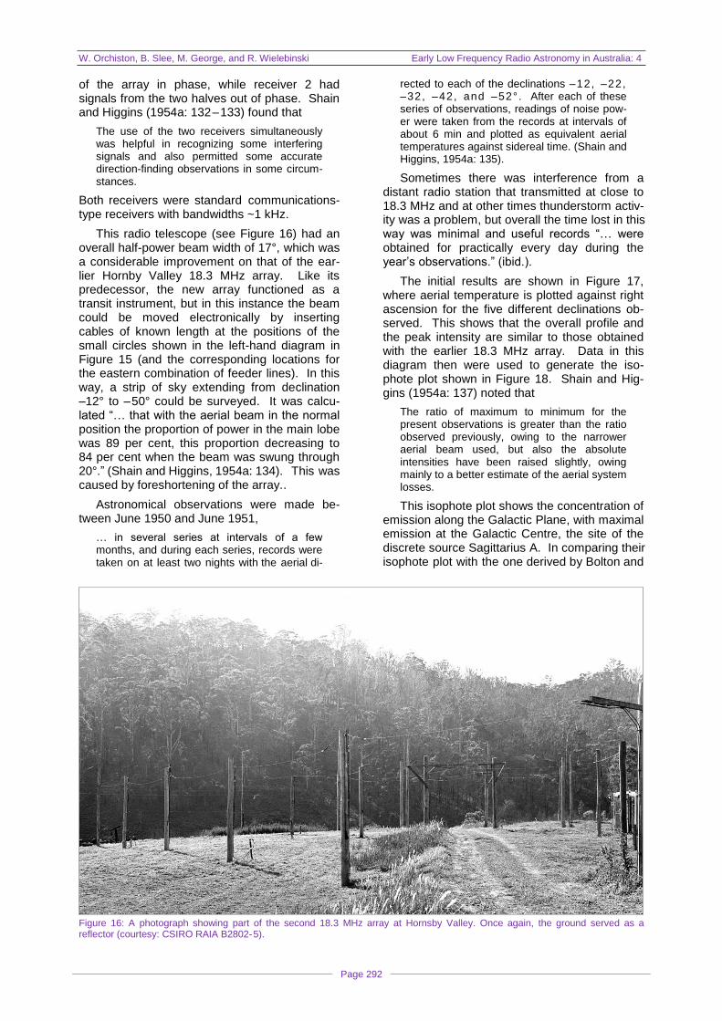
Figure 16: A photograph showing part of the second 18.3 MHz array at Hornsby Valley. Once again, the ground served as a reflector (courtesy: CSIRO RAIA B2802-5).


Page 293

Figure 17: Plots of equivalent aerial temperature against right ascension for five different declinations (after Shain and Higgins, 1954a: 136).

Figure 18: Contours of equivalent aerial temperature at 18.3 MHz plotted in galactic co-ordinates (after Shain and Higgins, 1954a: 137).

Westfold (1950), Shain and Higgins (1954a: 138) suggest that

Local differences in the shapes of the con-tours, for example in the regions near l = 80°, b = +20° and l = 305°, b = +5°, are probably

due to the effects of discrete sources.

Shain and Higgins (1954a: ibid.) noted a num-ber of other deviations in the contours, which they also attributed to discrete sources:

Since the objects giving rise to the localized in-creases in intensity must subtend an angle somewhat less than the beam width of the aerial and some at least correspond in position with discrete sources observed at higher frequencies, they have been called discrete sources; it should be remembered that they could have an angular size of several degrees. However, associated with some of these in-creases were short duration (order of 1 min)

fluctuations in the received intensity and, as discussed later, this observation suggested that some at least of the discrete sources would subtend angles of the order of 1° or less.

A careful analysis of the observational results produced a total of 37 discrete sources, and these are listed below in Table 1 and numbered following the scheme suggested by Mills (1952), where the hour of right ascension is followed by the sign and tens of degrees of the declination, ―... so that the designation of a source gives an indication of its position.‖ (Shain and Higgins, 1954a: 141). In order to differentiate their own sources from those detected by Mills, Shain and Higgins prefixed their sources with an ‗S‘ (thus S00–1, etc.). In commenting on entries in this table, Shain and Higgins (1954a: 141) noted that


Page 294

Table 1: Discrete sources observed at 18.3 MHz (after Shain and Higgins, 1954a: 140).

Source (S)

R.A. (hr min)

Decl. (°)

l (°)

b (°)

Flux Density (S) (10 – 23W m – 2 Hz) – 1 )

Level (L = 25+log10S)

Notes

00–1 00 23 –19 65 –81 1500 3.2

01–2 01 34 –20 150 –75 1100 3.0

03–4 03 24 –41 211 –54 350 2.5

04–2 04 22 –21 185 –39 700 2.8

05–4 05 12 –45 217 –35 350 2.5

06–1 06 05 –18 192 –16 1000 3.0

06–3 06 22 –33 209 –18 350 2.5

06–5 06 21 –51 227 –24 850 2.9

07–1 07 10 –18 199 –02 1200 3.1

08–4 08 20 –43 228 –03 700 2.8

09–1 09 23 –12 214 +28 400 2.6

09–3 09 20 –34 234 +12 700 2.8

09–5 09 55 –53 246 +02 800 2.9

10+1 10 45 +16 199 +61 1300 3.1

10–1 10 20 –10 224 +39 800 2.9

12+1 12 30 +11 262 +73 1100 3.0

12–0 12 53 –01 277 +61 4100 3.6 Intensity uncertain: confusion with S12–1

12–1 12 24 –14 263 +47 1500 3.2

13–2 13 20 –22 284 +40 2000 3.3

13–3 13 44 –33 285 +27 650 2.8

13–4 13 25 –43 279 +18 5300 3.7 Centaurus A

13–5 13 00 –58 273 +05 3300 3.5 Declination uncertain

14–4 14 45 –42 293 +15 5300 3.7

15–1 15 21 –16 317 +31 1000 3.0

15–6 15 35 –61 290 –05 6300 3.8 Declination uncertain

16–3 16 02 –39 308 +08 3800 3.6

18–2 18 20 –28 332 –09 5700 3.8

19+0 19 30 +02 08 –10 1100 3.0

19–2 19 40 –20 349 –23 650 2.8

20+x 20 02 +x -- -- (660000) (4.8) Influenced by Cygnus A?

20–4 20 06 –47 320 –34 350 2.5

21–1 21 20 –15 05 –42 1400 3.1

21–2 21 50 –25 354 –52 500 2.7

21–3 21 05 –30 344 –44 800 2.9

21–5 21 56 –52 311 –51 250 2.4

23–2 23 20 –25 05 –72 1550 3.2

23–5 23 30 –51 295 –64 250 2.4

Figure 19: The galactic distribution of discrete sources detected at 18.3 MHz, compared with those recorded by Mills at 101 MHz (after Shain and Higgins, 1954: 142).


Page 295

In general, for all the sources, positions could be assigned only roughly, with an estimated probable error of up to 5° for the weaker sources, although the uncertainty was some-what lower for the stronger sources. Similarly, the estimated probable errors in the intensities vary from about ±20 per cent, for the strongest to a factor of 2 for a few of the weakest sources.

With these concerns about positional accu-racy in mind, Shain and Higgins then plotted the distribution of these discrete sources in galactic co-ordinates, as shown in Figure 19. Source intensities were plotted using the values of ‗L‘ included in Table 1, with the solid lines and the dashed lines indicating the limits of the array‘s maximum and half-power points during the sur-vey. Also shown in this plot are the positions of discrete sources detected by Mills (1952) at 101 MHz from the Badgerys Creek field station. Sources that probably were detected in both sur-veys have dashed lines drawn around them.

Shain and Higgins then analysed their 18.3 MHz sources using the same method that had been adopted by Mills (ibid.), namely:

The logarithm of the number of sources with level L or greater is considered as a function of L. If there is a random distribution of a large number of sources, this function should be a straight line having a slope –1.5. (Shain and Higgins, 1954: 142).

When they plotted their sources (Figure 20), Shain and Higgins, found that they lay on a straight line with a slope of –1.1, which was similar to Mills‘ results. Then, upon carrying out further analyses of their sources, Shain and Hig-gins found that sources lying >18° from the galactic plane did have a slope of –1.5, while a figure of –1.3 was obtained for sources nearer the galactic plane, indicating that sources locat-ed at >18° ―... are distributed homogeneously whereas the ... [remaining sources] include some other class of source.‖ (Shain and Higgins, 1954: 143). They do not speculate on the nature of these ‗anomalous‘ sources.

Shain and Higgins also tried to use scintil-lations to investigate the angular sizes of their sources. They noticed that

Soon after recording began it was noticed that there were often irregular fluctuations in inten-sity at times when it appeared that a discrete source was passing through the aerial beam, although there were some sources which were rarely, if ever, seen to fluctuate in intensity. (Shain and Higgins, 1954: 143–144).

Scintillation indices were then calculated for 12 sources and plotted as a function of month of the observations (Figure 21) and the time when the observations were made (Figure 22, where the dashed curve shows the diurnal variation of the scintillation index determined by Ryle and Hewish (1950) for four northern sources).

Figure 20: A plot of L versus Log1 0 N for all sources between –04° and –60° (after Shain and Higgins, 1954: 143).

As Shain and Higgins (1954: 145–146; our italics) noted,

Both figures show a considerable scatter in the values of scintillation index. Although high values ... have not been observed during the winter nor during the midday and afternoon hours, this does not imply marked seasonal and diurnal variations since the sources with high scintillation indices have not been observ-ed at these times. In fact, no significant trends can be deduced from these data ... and there

are wide differences in the scintillation indices for different sources, even when observed at approximately the same time of day in the same season.

Figure 21: A plot of scintillation indices versus month of observations for 12 sources (after Shain and Higgins, 1954: 145).

Figure 22: A plot of scintillation indices versus time of observations for 12 sources (after Shain and Higgins, 1954: 145).


Page 296

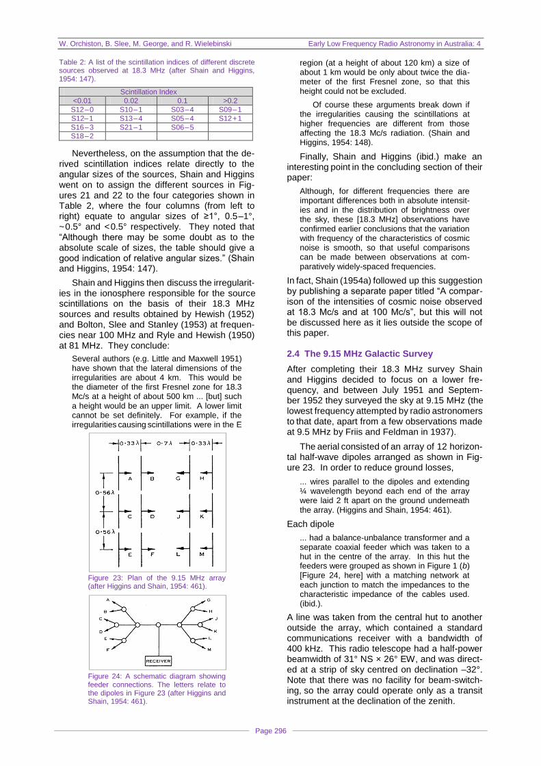
Table 2: A list of the scintillation indices of different discrete sources observed at 18.3 MHz (after Shain and Higgins, 1954: 147).

Scintillation Index

<0.01 0.02 0.1 >0.2

S12–0 S10–1 S03–4 S09–1

S12–1 S13–4 S05–4 S12+1

S16–3 S21–1 S06–5

S18–2

Nevertheless, on the assumption that the de-rived scintillation indices relate directly to the angular sizes of the sources, Shain and Higgins went on to assign the different sources in Fig-ures 21 and 22 to the four categories shown in Table 2, where the four columns (from left to right) equate to angular sizes of ≥1°, 0.5–1°, ~0.5° and <0.5° respectively. They noted that ―Although there may be some doubt as to the absolute scale of sizes, the table should give a good indication of relative angular sizes.‖ (Shain and Higgins, 1954: 147).

Shain and Higgins then discuss the irregularit-ies in the ionosphere responsible for the source scintillations on the basis of their 18.3 MHz sources and results obtained by Hewish (1952) and Bolton, Slee and Stanley (1953) at frequen-cies near 100 MHz and Ryle and Hewish (1950) at 81 MHz. They conclude:

Several authors (e.g. Little and Maxwell 1951) have shown that the lateral dimensions of the irregularities are about 4 km. This would be the diameter of the first Fresnel zone for 18.3 Mc/s at a height of about 500 km ... [but] such a height would be an upper limit. A lower limit cannot be set definitely. For example, if the irregularities causing scintillations were in the E

Figure 23: Plan of the 9.15 MHz array (after Higgins and Shain, 1954: 461).

Figure 24: A schematic diagram showing feeder connections. The letters relate to the dipoles in Figure 23 (after Higgins and Shain, 1954: 461).

region (at a height of about 120 km) a size of about 1 km would be only about twice the dia-meter of the first Fresnel zone, so that this height could not be excluded.

Of course these arguments break down if the irregularities causing the scintillations at higher frequencies are different from those affecting the 18.3 Mc/s radiation. (Shain and Higgins, 1954: 148).

Finally, Shain and Higgins (ibid.) make an interesting point in the concluding section of their paper:

Although, for different frequencies there are important differences both in absolute intensit-ies and in the distribution of brightness over the sky, these [18.3 MHz] observations have confirmed earlier conclusions that the variation with frequency of the characteristics of cosmic noise is smooth, so that useful comparisons can be made between observations at com-paratively widely-spaced frequencies.

In fact, Shain (1954a) followed up this suggestion by publishing a separate paper titled ―A compar-ison of the intensities of cosmic noise observed at 18.3 Mc/s and at 100 Mc/s‖, but this will not be discussed here as it lies outside the scope of this paper. 2.4 The 9.15 MHz Galactic Survey

After completing their 18.3 MHz survey Shain and Higgins decided to focus on a lower fre-quency, and between July 1951 and Septem-ber 1952 they surveyed the sky at 9.15 MHz (the lowest frequency attempted by radio astronomers to that date, apart from a few observations made at 9.5 MHz by Friis and Feldman in 1937).

The aerial consisted of an array of 12 horizon-tal half-wave dipoles arranged as shown in Fig-ure 23. In order to reduce ground losses,

... wires parallel to the dipoles and extending ¼ wavelength beyond each end of the array were laid 2 ft apart on the ground underneath the array. (Higgins and Shain, 1954: 461).

Each dipole

... had a balance-unbalance transformer and a separate coaxial feeder which was taken to a hut in the centre of the array. In this hut the feeders were grouped as shown in Figure 1 (b) [Figure 24, here] with a matching network at each junction to match the impedances to the characteristic impedance of the cables used. (ibid.).

A line was taken from the central hut to another outside the array, which contained a standard communications receiver with a bandwidth of 400 kHz. This radio telescope had a half-power beamwidth of 31° NS × 26° EW, and was direct-ed at a strip of sky centred on declination –32°. Note that there was no facility for beam-switch-ing, so the array could operate only as a transit instrument at the declination of the zenith.


Page 297

As might be expected at 9.15 MHz, interfer-ence from atmospherics and radio stations was an issue, and this is clearly illustrated in Figure 25. But at times when such interference was absent and ionospheric absorption was small, ―… a background intensity, which varied with sidereal time, was observed consistently and this was undoubtedly due to cosmic noise.‖ (Higgins and Shain, 1954: 460). Most of the useful obser-vations were carried out between midnight and sunrise, the objective being ―… to obtain as large a number of records as possible … [even if] only an hour‘s duration … In the course of a year suf-ficient samples to cover a full sidereal day could be obtained.‖ (Higgins and Shain, 1954: 463).

When combined, and corrected for ionospher-ic absorption at 9.15 MHz, these drift scans show-ed clear evidence of galactic plane emission (see Figure 26), but Higgins and Shain (1954: 464–465) cautioned that ―… a contribution from atmospherics to the received noise … cannot be completely ruled out … [although it] must be very small.‖

Higgins and Shain (1954) noted that the smoothed curve plotted in Figure 26 is similar to their 18.3 MHz curve and the one for 100 MHz, although the peak intensities differ significantly, and this is illustrated in Figure 27. However, the 18.3 and 100 MHz curves in this figure are calcu-

Figure 25: A record made on 23 August 1951 showing interference caused by atmospherics and radio stations. Atmospherics, which appear on the record as spikes, are very frequent at about 0230 hr, while radio station interference is strong at around 0240 hr. Both diminish after 0400 and the record is largely clear of interference until after 0410. The gradual drop in received power between 0400 and 0500 represents a genuine decline in cosmic noise intensity (after Higgins and Shain, 1954: 463).

Figure 26: Plots of equivalent aerial temperature against sidereal time for all successful observations, and corrected where necessary for the effects of ionospheric absorption. The curve is drawn through hourly averages, except for the dashed section where there are inadequate data. The accuracy of the solid curve is estimated to be better than 10%, and the dashed section ~20% (after Higgins and Shain, 1954: 466).


Page 298

Figure 27: A comparison of the equivalent aerial temperatures at three different frequencies, 9.15 MHz (a), 18.3 MHz (b), and 100 MHz (c) (after Higgins and Shain, 1954: 467).

lated values, as Higgins and Shain (1954: 466) explain:

The equivalent aerial temperature is the aver-age, weighted according to the aerial sensi-tivity in different directions, of the brightness temperatures over the visible sky. If observed equivalent aerial temperatures are available for a single lobe aerial, aerial A, say, having a comparatively small beam width, it is possible to determine the equivalent temperature that would be observed by a broader-beamed aer-ial by taking suitably weighted averages of the equivalent temperatures seen by aerial A when pointed in appropriate directions. This proced-ure was adopted to obtain the equivalent aerial temperatures that would have been observed at 18.3 Mc/s and at 100 Mc/s with an aerial having the same directivity (and side lobes) and pointed in the same direction as that used for the 9.15 Mc/s observations.

It is these curves that are plotted in Figure 27.

When Higgins and Shain plotted the maxi-mum and minimum values of equivalent aerial temperature shown in Figure 27 against frequen-cy (see Figure 28) they found that the points followed the relation

T f–2.8

(1)

Figure 28: A plot of minimum and maximum equivalent aerial temperatures (dots and circles, respectively) versus frequency (after Higgins and Shain, 1954: 468).

where T (in K) is the minimum equivalent temp-erature observed at a frequency f (in MHz).

Higgins and Shain also examined the minor irregularities in the 9.15 MHz curve plotted in Figure 27, and used the existence of discrete sources to explain these:

Calculations showed that passage of the aerial beam over discrete sources previously observ-ed at 18.3 Mc/s could account for these bumps at 18.3 Mc/s, and the presence of similar bumps at 9.15 Mc/s suggests that discrete sources are contributing appreciably to the radiation at 9.15 Mc/s. No accurate evaluation of source intensities can be made, but it appears that at 9.15 Mc/s they stand out against the background at least as clearly as at 18.3 Mc/s, possibly more so. (Higgins and Shain, 1954: 468).

In the concluding pages of this pioneering paper, Higgins and Shain (1954: 468) note that

Quantitatively, at least, the 9.15 Mc/s results fit the assumptions of an origin in discrete sources together with an absorbing (at 9.15 Mc/s) disk of interstellar gas ... From Shain‘s result [at 18.3 MHz] it would be expected that near the galactic centre the optical depth for 9.15 Mc/s radiation would be greater than unity for latitudes within 10° of the galactic equator. This could then account for the com-paratively low value of the maximum temper-ature at 9.15 Mc/s ...

Meanwhile, these results ―... are in accordance with what would be expected on current theoret-ical ideas.‖ (Higgins and Shain, 1954: 470).

2.5 The Positions of 18.3 MHz Solar Bursts

In 1959 Shain and Higgins published a paper about the positions of solar bursts observed with the 19.7 MHz Shain Cross at the Fleurs field station. What interests us here is that this paper also includes data on solar bursts observed in 1950–1951 with the second 18.3 MHz array at Hornsby Valley, and we discuss these here.

Because the 18.3 MHz aerial was a linear array (not a ‗Shain Cross‘), the positions of solar bursts could be measured only in one coord-inate. With this caveat in mind, Table 3 lists the derived positions of 18.3 MHz bursts recorded at Hornsby Valley in the course of the galactic observations. Note, however, that these posi-tions, which are listed to the nearest 5′, have an uncertainty of ±0.3° because of problems in est-imating atmospheric refraction. Furthermore, the ‗Optical Regions‘ (using numbers listed in the Quarterly Bulletin of Solar Activity) are those most likely to have been associated with the radio events, and ‗F‘ indicates that a flare occurred when the radio observations took place.

When data listed in the second and fourth columns in this table are plotted (Figure 29), we see that there is a strong correlation between the


Page 299

two parameters, although this is partly due to observational selection in that optical regions were chosen to fit the radio data. Nonetheless,

… we deduce that in 1950–1951 the 18.3 Mc/s sources were at a radial distance of 3.5R

from the centre of the Sun … although

this value is rather uncertain because of the scatter of the points and the basic uncertain-ties in identifying the optical sources. (Shain and Higgins, 1959: 367).

Yet Potts Hill data available at 97 MHz at that time tended to confirm the 18.3 MHz heights, and indicate that

... the sources of emission were rather higher in the corona than might have been expected on the basis of the Baumbach-Allen model of the corona … (Shain and Higgins, 1959: 357).

As we shall see in a later paper in this series, the 19.7 MHz results obtained at Fleurs field station subsequently would confirm this conten-tious Hornsby Valley result. 2.6 The Pre-Discovery of Jovian Decametric Emission

There is one final aspect of the Hornsby Valley research that deserves to be told and this is the serendipitous ‗pre-discovery‘ of Jovian decamet-ric emission.

As we have seen, terrestrial interference was a common problem encountered by radio astron-omers who worked at low frequencies, and Shain and Higgins probably regarded this as a nui-sance and a distraction. This, too, was the in-itial attitude of the U.S. duo of Bernard Flood Burke (b. 1928; Figure 30) and Kenneth Linn Franklin (1923–2007) when they encountered ‗in-terference‘ while conducting research with the Carnegie Institution of Washington‘s 22 MHz Mills Cross-type radio telescope (Figure 31)

6 that

was located at Seneca, Maryland, ~32 km north-west of Washington DC. However, when they analysed their ‗interference‘ they discovered, to their surprise, that it originated from Jupiter. Accordingly, in 1955 they announced their discov-ery in a paper published in the Journal of Geo-physical Research. This was not a journal that habitually was read by radio astronomers, but the magnitude of this discovery—the first detec-tion of radio emission from a planet in our Solar System other than the Earth—guaranteed that it found its way into Nature (Radio emission from Jupiter, 1955), and this gave it a very wide audience (cf. Franklin and Burke, 1956; Frank-lin, 1959).

Franklin (1959: 37–38) later described the ex-citement of the discovery. Early in 1955 he and Burke were observing near the Crab Nebula (Taurus A), and the records

… showed the characteristic hump as the Crab Nebula passed through the pencil beam

Table 3: 18.3 MHz solar bursts observed at Hornsby Valley in 1950–1951 (adapted from Shain and Higgins, 1959: 361).

Date HA r –HA s*

(′) Optical Region

HA o–HA s (′)

▪1950 ▪

Nov 16 00 8 F 00

Nov 17 +20 ---- ----

▪1951▪

Jan 30 +10 7 +04

Feb 01 +40 7 F +09

Feb 02 +20 5 F +06

Feb 24 –05 13 –01

Mar 16 –40 18 –13

Mar 17 –25 18 –12.5

Mar 18 –35 18 –12

Mar 19 +10 18 –09.5

Mar 20 –10 18 –07

Mar 22 –10 18 –0.5

Mar 24 +05 18 +05.5

Mar 25 +50 18 +08.5

Mar 26 +80 18 +11

* Key: HA r = Hour angle of the Radio Source HA s = Hour angle of the Sun HA o = Hour angle of the Optical Region

… followed by a smaller hump … attributed to IC443. At times the records exhibited … inter-ference … [after] the passage of the two known sources. This intermittent feature was curious, and I recall saying once that we would have to investigate the origin of that inter-ference some day. We joked that it was probably due to the faulty ignition of some farm hand returning from a date.

[Later] … Burke assembled all the records of the Taurus region for the first three months of 1955 ... [and was] startled to find that the interference always occurred at almost the same sidereal time. A strange rural romance this was turning out to be! As spring drew nearer, our swain was returning home earlier

Figure 29: A plot of the observed E-W displacements from the centre of the Sun of the 18.3 MHz sources listed in Table 3 (after Shain and Higgins, 1959: 362).


Page 300

Figure 30: Bernard Burke (left), and Radio Jove‘s Chuck Higgins (right)—no relation to Australia‘s Charlie Higgins—meet in April 2005 during the dedication ceremony of an historical marker on the 50

th anniversary of the discovery of

Jovian decametric emission near Seneca, Maryland (http:// radiojove.gsfc.nasa.gov/library/newsletters/ 2009Apr/).

and earlier, each evening ...

The late Howard Tatel, a man of many parts, was present in the Laboratory ... [and] somewhat facetiously suggested to Burke and me that our source might be Jupiter. We were amused at the preposterous nature of this re-

mark, and for an argument against it I looked up Jupiter‘s position in the American Ephem-eris and Nautical Almanac. I was surprised to find that Jupiter was just about in the right place, and so was Uranus. Here was some-thing which needed clearing up ....

[After investigating and eliminating Uranus] I began to plot the right ascensions of Jupiter. As I plotted each point, Burke, who was watch-ing over my left shoulder, would utter a gasp of amazement. Each point appeared right be-tween the boundary lines representing the be-ginning and end of each event. The meaning was exquisitely clear: these events were re-corded only when Jupiter was in the confines of the narrow principal beam of the Mills Cross. Not only did the source have the same direction in space as Jupiter, but it also exhibited the same change of direction as Jupiter did its retrograde loop of 1955. No other ob-ject could satisfy the data: the source of the intermittent radiation was definitely associated with Jupiter.

Among the international colleagues Burke and Franklin contacted following their discovery was Alex Shain in Australia, and ―He set up operations at 19 MHz and confirmed that Jupiter was busy.‖ (Franklin, 1983: 255). But Shain actually did more than this. He recalled those periods of intense 18.3 MHz ‗static‘ that he and Higgins had recorded (e.g. see Figure 32) at the Hornsby Valley field station in 1950 and 1951, and he decided to revisit these.

Figure 31: A view looking along one of the arms of the 22 MHz Mills Cross at Seneca, Maryland. Each arm was 624 metres long, and contained 66 dipoles (courtesy: Carnegie Institution of Washington).


Page 301

Figure 32: Examples of 18.3 MHz Jovian bursts recorded at Hornsby Valley in 1950–1951. Dates of the observations are 17 October 1950 (top) and 29 October 1950 (bottom) (adapted from CSIRO RAIA: B3719-13).

Shain (1955b) reported his initial results in a paper published in Nature on 29 October 1955, a mere four months after the appearance of Burke and Franklin‘s ‗discovery paper‘. He not-ed that there were two chronological series of Hornsby Valley records:

(1) October 1950–April 1951, when the beam-width of the aerial was 17°, and Jovian emission was recorded on about half of all days when the antenna was directed towards Jupiter and terrest-rial interference was absent. Moreover,

For some of these records more accurate direction-finding was possible using a split-beam technique, and these records proved that the position of the source was within ±1° of Jupiter. (Shain, 1955b: 836).

This was clear confirmation of Burke and Frank-lin‘s results.

(2) 15 August–2 October 1951, when the array had been modified so that it was narrow in dec-lination but very broad in hour angle. This allow-ed continuous observations for nearly 8 hours, which encompassed almost one complete rota-tion of Jupiter. During this period, Jovian bursts were recorded on 27 of the 30 days when suit-able records were obtained.

However,

A most interesting new fact coming out of the examination of these records was the very close relation between the times of occurrence of bursts and the rotation of Jupiter. (ibid.).

Jupiter exhibits differential rotation, with the pol-ar regions rotating more slowly than the equa-torial zones. Accordingly there are two different recognised periods of rotation, which are refer-red to as System I (9h 50m 30.003s) and Syst-em II (~9h 55m 40.632s). When Shain plotted the occurrence times of Jupiter bursts against the Jovian longitude of the central meridian for the two different Systems he found two distinct patterns—as illustrated in Figure 33. Jovian

bursts varied widely in Joviocentric longitude in the System I plot, but were almost aligned under one another in the System II plot, indicating that the rotation period (P) of the source of the emis-sion was close to that of System II. Upon allow-ing for the slight negative drift in the System II plot, Shain (1957: 398) was able to derive a value of

P = 9h 55m 13 ± 5s

for the source. Furthermore, when a histogram of the Joviocentric longitude of the emission was plotted (Figure 34) it showed that

… for a band of longitudes centred on 67° and extending from 0° to 135°, the frequency of occurrence was much greater than outside this band. This suggests an origin in a very localized source on Jupiter. Since there are about 120 rotations of Jupiter during the period of observations on which the figure is based, the probability that the effect observed is due to chance is extremely small. (Shain, 1955b).

But Shain took his analysis one step further and actually identified the source of the emis-sion! He noted that the Jupiter Section of the British Astronomical Association had provided him with a drawing by E.J. Reece (Figure 35) that showed a conspicuous white spot

… at the boundary between the South Temp-erate Zone and the South Temperate Belt, which was observed for several months, [and] had an observed rotation period of 9

h 55

m 13

s,

that of the radio source … although the ident-ification is not proved beyond all doubt, it seems very probable that this visually-disturbed region was responsible for the radio radiation

... (Shain, 1957: 398–399; our italics).

Shain (1956) elaborated on these initial in-vestigations in a more detailed paper that was published in the Australian Journal of Physics in 1956. In a preamble, he noted that

During the rapid development of radio astronomy in the last 10 years, the question has some-


Page 302

Figure 33: Periods of occurrence of 18.3 MHz emission in 1951 plotted against Joviocentric longitude (after Shain, 1957).

times been raised as to whether radiation from any of the planets could be detected. The de-tection of thermal radiation would appear to be at present impracticable, but it has been sug-gested (Higgs 1951) that electrical discharges analogous to terrestrial lightning flashes may occur in the atmosphere of Venus and that radiation from such discharges may be detect-able. In 1955, however, came the quite un-expected announcement by Burke and Frank-lin (1955) that very intense radiation at 22 Mc/s had been received from … Jupiter ...

Upon discussing the 18.3 MHz Hornsby Valley galactic survey records from 1950–1951 Shain explained that

… a watch was kept for peculiarities on the records, especially for bursts of solar noise and for variations caused by abnormal iono-spheric attenuation. Quite frequently there was interference from atmospherics and radio stations; thus no particular significance was attached to the occurrence of occasional groups of bursts during the night. (Shain, 1956: 62; our italics).

Figure 34: Histogram of the occurrence frequency of 18.3 MHz Jovian emission plotted against System II Joviocentric longitude (after Shain, 1956: 68).

Figure 35: A drawing of part of Jupiter‘s disk on 29–30 Nov-ember 1951 UT. The radio emission was observed only until 2 October, but its extrapolated longitude on 29 November is 354° the precise position of the right hand white spot (after Shain, 1956: 70).

The focus was very much on the distribution of galactic emission and discrete sources and much less so on solar emission and atmospherics at 18.3 MHz, so there simply was no time (and perhaps inclination) to investigate these occas-ional groups of anomalous bursts—which were dismissed as interference.

In this paper, Shain (1956: 62) also explains how it was that the 1951 Jovian observations were possible:

In June 1951 part of the original aerial had been dismantled, but a single receiver was used to measure the noise picked up by the remaining ten dipoles, which had an aerial diagram narrow in the north-south direction but very broad in the east-west direction.

Although it certainly was not anticipated at the time, fortuitously this aerial proved to be ideal for the monitoring of Jupiter over the course of almost one entire rotation each time an observa-tion was recorded. Thanks to this the Joviocen-tric longitude distribution of the emission could be investigated and this in turn suggested that much of the emission came from a single source.

During the first suite of observations, made with the full array, sometimes the sound of what later proved to be Jovian bursts was noted:

Notes written on some records indicate that many bursts sounded like ―swishes‖ (similar to solar bursts, with which they were confused) and therefore the recorder followed these noise variations faithfully. On some other occasions there were sounds suggesting the presence of short impulses which the recorder would not follow. (Shain, 1956: 63).

So, unknowingly, Shain and Higgins were the first to hear Jovian bursts (and record radio emis-sion from another planet in our Solar System).

In his detailed paper, Shain also comments on the primary emission peak shown in Figure 33, and he provides several explanations for it, assuming all along that it is a single source of radiation on the basis that ―… the emitting reg-


Page 303

ion was probably small in extent to give an ―emis-sion polar diagram‖ of much less than 180°.‖ (Shain, 1956: 69). Surprisingly, there is no sug-gestion that the ‗primary peak‘ may comprise three overlapping Gaussian curves associated with strong sources located at Joviocentric long-itudes of ~40°, 70° and 110°, plus a fourth, very much weaker, source at ~315°.

An interesting new section in Shain‘s 1956 paper relates to three Jovian satellite occulta-tions that occurred when the radio observations were made. The records were examined

… to see whether there were any marked changes, corresponding to occultations, which would help to locate the source. On one occasion there was no effect at all, and on a second there was only a very doubtful sug-gestion of an occultation …

On the third occasion, during the transit of Satellite II on September 24, there was a sudden cessation of the noise as the satellite reached the meridian of the source, at 03

h 10

m.

This may have been a coincidence, since the noise had already been received for over 2 hr, but on one or two other days noise had been received continuously for over 4 hr. At 03

h

10m the source was still within 25° of the cen-

tral meridian and as there was weak noise again 32

m later, there is a reasonable probab-

ility that the sudden decrease in intensity was due to an occultation of the source.

All of this is academic of course, if more than one primary source of emission was involved.

Finally, in another expansion of the material presented in his Nature paper, Shain (1956: 71) discusses how variations in the intensity of the Jovian emission can potentially be used to in-vestigate

… propagation conditions in interplanetary space near the plane of the ecliptic and espec-ially along ray paths that pass near the Sun … The observations described in this paper did not cover a very long period of time, but in the course of the year there were noteworthy changes in the characteristics of the radiation from Jupiter.

The changing duration of bursts is discussed as a possible mechanism that can be used to explore scattering in the outer corona. 3 DISCUSSION

3.1 The 1952 URSI Congress

Every three years the International Union of Radio Science (or Union Radio Science Inter- nationale, URSI) holds a Congress in a different international city. In recognition of Australia‘s important contributions to ionospheric research and radio astronomy a decision was made to hold the 1952 meeting in Sydney. This was the first time a major URSI meeting had been held outside Europe or North America, and was fitting rec-

Figure 36: During the URSI visit to Hornsby Valley, Alex Shain (on the extreme right) discusses chart records with (left to right) Francis Graham Smith, Robert Hanbury Brown, Jim Hindman, Charlie Higgins, Joe Warburton and unidentified person X (mostly obscured) (courtesy: CSIRO RAIA 2842-133).

ognition of Australia‘s important place in interna-tional radio science (see Robinson, 2002).

An important component of each URSI Con-gress was the field trips, and in 1952 visits were arranged to RP‘s Dapto, Hornsby Valley and Potts Hill field stations. The Hornsby Valley visit offered Shain and Higgins an excellent chance to showcase their low frequency research and instrumentation to not only their RP colleagues (Chris Christiansen, Jim Hindman, and Joe War-burton), but also the leading British radio astron-omers, Francis Graham Smith and Robert Han-bury Brown, and Marius Laffineur from France.

Fortunately, fair weather greeted those who chose the Hornsby Valley field trip, which was documented by RP‘s photographers.

7 Figures

36 and 37 show Shain and Higgins discussing their observations with Graham Smith, Hanbury Brown and their RP colleagues, while Figure 38 shows the whole group assembled outdoors at the field station.

Figure 37: From left to right, Joe Warburton, Francis Graham Smith, Charlie Higgins, Robert Hanbury Brown, Jim Hindman (partly obscured), unidentified person X (almost totally obscur-ed) and Alex Shain examine some of the chart records (cour-tesy: CSIRO RAIA 2842-132).


Page 304

Figure 38: Radio astronomers from the 1952 URSI Congress shown at the Hornsby Valley field station. Alex Shain is on the extreme left, seated between Robert Hanbury Brown and unidentified person X. Francis Graham Smith (glasses) and unidentified person Y are at the end of the table. Opposite Shain and Hanbury Brown are (from left to right): Joe Warburton, Marius Laffineur (standing), Charlie Higgins (standing), Chris Christiansen and Jim Hindman. The antennas in the background formed part of the 9.15 MHz array (courtesy: CSIRO RAIA 2842-131).

3.2 Other Research in Radio Astronomy Conducted at Hornsby Valley

Along with Dr Alexander in New Zealand (Orch-iston, 2005a), RP‘s Ruby Payne-Scott (1912–

Figure 39: Ruby Payne-Scott (cour-tesy: CSIRO RAIA).

1981; Figure 39; Goss and McGee, 2010; Goss, 2013) was a pioneering female radio astrono-mer. In 1947 she was carrying out solar re-search at Dover Heights field station, sharing the blockhouse and Yagi antennas with John Gatenby Bolton (1922–1993; Robertson, 2015), Gordon James Stanley (1921–2001; Kellermann et al., 2005) and Owen Bruce Slee (b. 1924; Orchiston, 2004; 2005b) who were researching what at the time were termed ‗radio stars‘ (Rob-ertson et al., 2014). However, tension soon arose between Bolton‘s group and Payne-Scott.:

Part of the problem was that both groups often wanted to use the same piece of equipment at the same time, or one group wanted to carry out routine maintenance which might create radio interference for the other group. With space in the blockhouse limited, the two groups were getting in each other‘s way.

The main problem however was a person-ality clash between Bolton and Payne-Scott ...


Page 305

[and] it is doubtful whether he had ever come across anyone like her. Most of his life had been spent in a largely all-male environment ... [Moreover,] Ruby had forthright views on all sorts of issues such as politics and women‘s rights. Many of the young Radiophysics staff held left-wing views, but Payne-Scott went one step further. She and her husband were card-carrying members of the Communist Party, earning her the nickname ‗Red Ruby‘. (Robert-son, 2015: 65).

Eventually, the feud between the two came to a head, and Payne-Scott was forced to leave Dover Heights.

At the end of 1947 she transferred to Horns-by Valley, where she set up single 60, 65 and 85 MHz Yagi antennas (Figure 40). From Jan-uary through to September 1948 she used these, plus an 18.3 MHz broadside array and Kerr and Shain‘s 19.8 MHz Moon-bounce rhom-bic antenna, to study solar emission. Most of the observations were made at 60 and 85 MHz, and crossed Yagis were used at 85 MHz to investigate the polarization of the solar bursts.

From these observations Payne-Scott (1949: 215) identified two different types of variable high-intensity radiation: ‗enhanced radiation‘ and ‗unpolarized bursts‘. With the first of these,

The intensity reaches a high level and remains there for hours or days on end; there are con-tinual fluctuations in intensity, both long-term and short-term. The short-term increases are

somewhat similar to [isolated] bursts … but usually have a lower ratio of maximum to background radiation. This type of radiation will be called ―enhanced radiation‖ ... Superimposed on it may be bursts … There may be short periods during which the polarization is in-definite, either because two sources of oppo-site polarization are superimposed or because the radiation is linearly or randomly polarized, but for the great part of its life the enhanced level shows circular polarization of one sense or the other. (Payne-Scott, 1949: 216–217).

Figure 41 shows an example of this ‗enhanced emission‘, which later was found to be charac-teristic of spectral Type IV solar emission.

The second type of solar radiation Payne-Scott investigated at Hornsby Valley was the ‗unpolarized bursts‘, which showed

… a very good correspondence on different frequencies, though their shapes and relative amplitudes may vary considerably … the closer the frequencies and the larger the bursts, the closer their relationship. Corresponding bursts do not appear to skip frequencies. Thus, if a burst appears on 95 and 19 Mc/s., there will be a corresponding burst on 60 Mc/s. ... A characteristic unpolarized burst shows a finite rise time, rounded top, and slow decay, remin-iscent of the transient response of a medium with a natural resonant frequency … There is no marked connexion between the rate of de-cay and the intensity of the burst … [but bursts recorded at 18.3 and 19.8 MHz] have a mark-

Figure 40: The 60 MHz and 85 MHz Yagi antennas (on the left) and the 19.8 MHz rhombic antenna (centre and right) used by Ruby Payne-Scott for her solar observations in 1948 (courtesy: CSIRO RAIA B1266-2).

Figure 41: An example of ‗enhanced emission‘ recorded on 30 August 1948 at 85 MHz. Observations were made with crossed Yagis and this chart record shows emission received with the horizontally-polarized aerial (after Payne-Scott, 1949: 218).


Page 306

edly slower decay rate … (Payne-Scott, 1949: 219–221).

This was important research, but since most of the solar emisson investigated by Payne-Scott was recorded at 60 or 80 MHz, it lies beyond the scope of this paper (but, for further details, see Goss and McGee, 2010; Orchiston et al., 2006). 3.3 Low Frequency Radio Astronomy and the Ionosphere

The focus of this paper is the radar and low fre-quency radio astronomy that was carried out at the Hornsby Valley field station, but atmospherics played a key role in allowing or preventing the later investigations, as we have seen. There-fore, it is not surprising that Shain and a visiting Indian radio astronomer, A.P. Mitra, also wrote papers on changes in the different levels of absorption in the ionosphere.

Mitra and Shain (1953) showed that

…although the D-region generally makes the greater contribution to the absorption of 18.3 Mc/s cosmic noise during daylight hours, the F-region may produce considerable attenu-

ation when 0F2 is high. (Shain, 1955a: 347).

Meanwhile, Shain (ibid.) noted that

During ionospheric storms 0F2 often departs

considerably from its usual value for short periods, and it would be expected that, for at least the largest increases, there would be corresponding increases in the attenuation of cosmic noise.

Finally, Mitra and Shain (1954) demonstrated that variations in 18.3 MHz ‗cosmic noise‘ could be used to detect short-term increases in D-region absorption following solar flares. 3.4 The Sequel: Fleurs

After completing the 9.15 MHz survey, Shain and Higgins were keen to develop a larger array with improved resolution, so they could continue their low frequency research, but there was a prob-lem. While Hornsby Valley was radio-quiet, and was accessible by car and rail from central Sydney, there simply was not enough relatively flat land for a much larger low frequency array.

8

Consequently, Shain (1952) recommended that their research should be transferred to an-other RP field station. Initially he favoured Bad-gerys Creek on the western outskirts of subur-ban Sydney (Site 1 in Figure 1), but for various reasons this did not happen. Instead it was the nearby Fleurs field station (Site 6 in Figure 1) that benefited from the eventual close down of the Hornsby Valley field station in 1955, and over the next decade or so Fleurs would play a leading role in international low frequency radio astronomy (e.g. see Orchiston and Slee, 2002;

2005a; Robertson, 1992). This will be the sub-ject of a later paper in this series on early Australian low frequency radio astronomy. 4 CONCLUDING REMARKS

During the late 1940s and early 1950s, the CSIRO‘s Division of Radiophysics field station at Hornsby Valley near Sydney was a world leader in low frequency radio astronomy, but the first research that occurred there was in radar astron-omy. This was carried out in 1947–1948 by Frank Kerr and Alex Shain, and built on pioneer-ing projects conducted in Hungary and the USA in 1946. Kerr and Shain made important contri-butions to our understanding of the ionosphere, and they also were the first to use radar tech-niques to pronounce on the nature of the lunar surface. After moving to the Potts Hill field sta-tion Kerr would build an international reputation through his H-line work, and he would never again conduct low frequency research in radio or radar astronomy. But, as a farewell to radar astronomy, in 1952 he published the hallmark paper, ―On the possibility of obtaining radar echoes from the Sun and planets‖, in the Pro-ceedings of the Institute of Radio Engineers.

Between May 1949 and June 1951 Alex Shain and Charlie Higgins built Hornsby Valley into the world‘s leading low frequency radio astronomy facility. They began with an ‗all-sky‘ survey at 18.3 MHz, and after upgrading the original transit array so that beam-switching was possible, were able to produce an isophote plot of galactic emission and a map showing the distribution of 37 discrete sources, a vast im-provement on what Karl Jansky was able to achieve at a similar frequency back in the 1930s. Through their Hornsby Valley work Shain and Higgins were able to significantly expand the frequency range of non-solar research at RP, which to that time had predominantly been con-ducted at around 100 MHz.

In June 1951, after completing their 18.3 MHz research, Shain and Higgins began a survey of emission at 9.15 MHz. They were able to detect galactic plane emission at this frequency, and infer the presence of discrete sources (although they lacked the resolution to investigate these). Note that 9.15 MHz would remain the lowest frequency at which radio astronomy was carried out until Ellis and Reber conducted their succ-essful 2.13 and 1.435 MHz surveys from Cam-bridge, Tasmania, in 1955 (see George et al., 2015b).

In addition to their galactic research, at a later date Shain and Higgins were able to exam-ine 18.3 MHz solar bursts detected at Hornsby Valley in 1950–1951, and show that the sources of these bursts were located somewhat higher in the corona than anticipated using the Baumbach-


Page 307

Allen model. This was a significant result.

Another significant Hornsby Valley result, and one that also was obtained belatedly, was the discovery that during their 1950–1951 galactic survey Shain and Higgins had in fact detected bursts from Jupiter on numerous occasions, but dismissed them as troublesome interference. It was only after Burke and Franklin announced their discovery of Jovian decametric emission in mid-1955 that Shain revisited the old Hornsby Valley chart records and was able to report these pre-discovery observations. Upon exam-ining these, he would claim that the emission came from a single source, with a rotation period of 9h 55m 13s (very close to System II). But he went further and suggested that the source was associated with a conspicuous white spot that was located on the boundary of the South Temperate Belt and South Temperate Zone. While these ideas were revolutionary at the time we now know they were simplistic—in 1955 no-one could ever have imagined that the Jovian decametric emission was associated with the magnetic torus between Jupiter and its anom-alous inner satellite Io. With the benefit of hind-sight, we can understand why Shain and Higgins failed to identify Jovian bursts in 1950–1951, but this should not prevent us from identifying this as one of RPs most notable ‗missed opportun-ities‘. Meanwhile, research on Jovian decametric emission would be avidly pursued by RP staff at the Fleurs field station, as a later paper in this series will document.

It is interesting that Shain never chose to examine any of the 9.15 MHz chart records from 1951–1952 for possible Jovian emission (or if he did, there is no mention of this in his published papers).

Because of the special problems that the ionosphere introduced for those conducting low frequency radio astronomy, it is no surprise that Shain and his Indian collaborator, A.P. Mitra, also wrote papers about ionospheric absorption that led to an improved understanding of the operation of the D-layer and the F-layer, inform-ation that was of interest to ionospheric scien-tists worldwide. In this way, the Hornsby Valley field station was able to enhance its reputation as an international centre of low frequency radio science, but as we have seen, it also contribu-ted briefly to 60–85 MHz solar radio astronomy through the research carried out there by Austra-lia‘s first female radio astronomer, the remarkable Ruby Payne-Scott, before she, too, transferred to the Potts Hill field station.

By the time the Hornsby Valley field station was closed, Frank Kerr, Alex Shain and Charlie Higgins had made important low frequency observations of the Moon and our Galaxy, and later some of them would use data from this

field station to make valuable contributions to low frequency solar and Jovian astronomy. Alex Shain and Charlie Higgins would then continue some of these investigations from Fleurs field station.

5 NOTES

1. In 1949, after ―… the biggest upheaval in Australian science in the country‘s history.‖ (Peter Robertson, pers. comm., 2015), the Australian Government‘s Council for Scientif-ic and Industrial Research (CSIR) was replac-ed by the Commonwealth Scientific and In-dustrial Research Organisation (CSIRO).

2. This is the fourth in a series of papers aimed at documenting early low frequency radio astronomy in Australia. The first two papers overviewed the activities of staff from the Division of Radiophysics, near Sydney (Orch-iston et al., 2015) and radio astronomers in Tasmania (George et al., 2015a). The third paper in the series was the first of the detail-ed case studies, and examined the research carried out by Ellis and Reber at the Cam-bridge field station near Hobart (George et al., 2015b).

3. Originally, the first and second authors of the present paper were employed by the Division of Radiophysics, and although they never worked at the Hornsby Valley field station, between them they personally knew all of the individuals whose research is discussed in this paper.

4. During this period RP also had field stations at Dover Heights (site 5 in Figure 1), Georges Heights (site 8), Penrith (site 15) and Potts Hill (site 16) and, in addition, research was carried out from the roof of the Radiophysics Laboratory (site 17). For summaries of the research conducted at these locations see Orchiston and Slee (2005a) and Robertson (1992).

5. Initially, the term ‗radio astronomy‘ did not exist, and those who researched ‗cosmic noise‘ and ‗solar noise‘ predominantly had backgrounds in radio or radar, not in astron-omy. It was only in 1948 that the term ‗radio astronomy‘ began to be used internationally (see Sullivan, 2009: 423–424), after being coined by Joe Pawsey and first mentioned in a letter he wrote in January 1948 (see Robert-son, 1992: 31).

6. In 1952 Australian radio astronomer, Bernard Yarnton Mills (1920–2011; see Mills, 2006) invented a new type of radio telescope that dramatically improved the resolution of radio telescopes (see Mills, 1963). Built in the shape of a cross, the E-W arm produced a N-S fan beam and the N-S arm an E-W fan beam. By electrically switching the signals from the two arms in phase and out of phase,


Page 308

the radio telescope produced a pencil beam where the two arms of the array intersected. Mills and Little (1953) constructed a proto-type ‗Mills Cross‘ at RP‘s Potts Hill field sta-tion in suburban Sydney (Wendt, Orchiston and Slee, 2011), and when this proved that the concept was viable, a new much larger Mills Cross was constructed in 1954 (Mills and Little, 1953) at the Fleurs field station, which is site 6 in Figure 1 (Orchiston and Slee, 2002; 2005a). The prototype Mills Cross and the later Mills Cross at Fleurs inspired the construction of other Mills Cross radio telescopes around the world, and one of the earliest of these was the Carnegie Institution‘s Mills Cross near Washington DC.

7. During the War years the CSIR‘s Division of Radiophyics established a Photographic Lab-oratory, staffed by professional photograph-ers, and over the years they assembled an outstanding pictorial record of early Austral-ian radio astronomy (see Orchiston, 2001; Orchiston et al., 2004).

8. An additional factor that hastened the aban-donment of the Hornsby Valley as a radio astronomy field station was a bushfire that swept through the region near the end of 1952 and destroyed buildings and equipment (Patricia Dewey, pers. comm., 2004; John Murray, pers. comm., 2004).

6 ACKNOWLEDGEMENTS

We are grateful to Mrs Patricia Dewey (Hornsby Historical Society) and John Murray (formerly Division of Radiophysics, CSIRO) for providing helpful information, and Professor Richard Strom (ASTRON) and Dr Peter Robertson (University of Melbourne) for commenting on the MS. We also wish to thank CSIRO Astronomy and Space Sciences for supplying Figures 2–7, 16 and 36–40, and the Carnegie Institution of Washington for permission to publish Figure 31. 7 REFERENCES

Bay, Z., 1946. Reflection of microwaves from the Moon. Hungarica Acta Physica, 1, 1–22.

Bolton, J.B., Slee, O.B., and Stanley, G.J., 1953. Galactic radiation at radio frequencies. VI. Low altitude scintillations of the discrete sources. Austral-ian Journal of Physics, 6, 434–451.

Bolton, J.B., and Westfold, K.C., 1950. Galactic radiation at radio frequencies. I. 100 Mc/s. survey. Australian Journal of Scientific Research, A3, 19–33.

Brown, L., 1999. Technical and Military Imperatives. A Radar History of World War II. London, Taylor

and Francis. Burke, B.F., and Franklin, K.I., 1955. Observations of

a variable radio source associated with the planet Jupiter. Journal of Geophysical Research, 60, 213–

217. Clark, T., 1980. How Diana touched the Moon. IEEE Spectrum, 17, 44–48.

DeWitt, J.H., and Stodola, E.E., 1949. Detection of radio signals reflected from the Moon. Proceedings of the Institute of Radio Engineers, 37, 229–242.

Franklin, K.I., and Burke, B.F., 1956. Radio obser-vations of Jupiter. Astronomical Journal, 61, 177.

Franklin, K.I., 1959. An account of the discovery of Jupiter as a radio source. Astronomical Journal, 64,

37–39. Franklin, K.L., 1983. The discovery of Jupiter bursts.

In Kellermann, K., and Sheets, B. (eds.). Seren-dipitous Discoveries in Radio Astronomy. Green

Bank, National Radio Astronomy Observatory. Pp. 252–257.

Friis, H.T., and Feldman, C.B., 1937. Multiple unit steerable antenna for short-wave reception. Pro-ceedings of the Institute of Radio Engineers, 25,

841–917. George, M., Orchiston, W., Slee, B., and Wielebinski,

R., 2015a. The history of low frequency radio astronomy in Australia. 2: Tasmania. Journal of Astronomical History and Heritage, 18, 14–22.

George, M., Orchiston, W., Slee, B., and Wielebinski, R., 2015b. The history of low frequency radio astronomy in Australia. 3: Ellis, Reber and the Cambridge field station. Journal of Astronomical History and Heritage, 18, 177–189.

Goss, W.M., and McGee, R., 2010. Under the Radar: The First Woman in Radio Astronomy: Ruby Payne-Scott. Springer.

Goss, W.M., 2013. Making Waves: The Story of Ruby Payne-Scott: Australian Pioneer Radio Astronomer. Springer.

Hewish, A., 1952. The diffraction of galactic radio waves as a method of investigating the irregular structure of the ionosphere. Proceedings of the Physical Society, A 214, 494–514.

Hey, J.S., 1973. The Evolution of Radio Astronomy. New York, Science History Publications.

Higgins, C.S., and Shain, C.A., 1954. Observations of cosmic noise at 9.15 Mc/s. Australian Journal of Physics, 7, 460–470.

Higgs, A.J., 1951. Radio astronomy. Science News, 21, 39–60.

Jansky, K.G., 1937. Minimum noise levels obtained on short wave radio receiving systems. Proceedings of the Institute of Radio Engineers, 25, 1517–1530.

Kellermann, K.I., Orchiston, W., and Slee, B., 2005. Gordon James Stanley and the early development of radio astronomy in Australia and the United States. Publications of the Astronomical Society of Australia, 22, 13–23.

Kerr, F.J., Shain, C.A., and Higgins, C.S., 1949. Moon echoes and penetration of the ionosphere. Nature, 163, 310–313.

Kerr, F.J., and Shain, C.A., 1951. Moon echoes and transmission through the ionosphere. Proceedings of the Institute of Radio Engineers, 39, 230–242

Kerr, F.J., 1952. On the possibility of obtaining radar echoes from the Sun and planets. Proceedings of the Institute of Radio Engineers, 40, 660–666

Kerr, F.J., 1984. The early days in radio and radar astronomy in Australia. In Sullivan, 1984, 133–145.

Little, C.G., and Maxwell, A., 1951. Fluctuations in the intensity of radio waves from galactic sources. Philosophical Magazine, 42, 267–278.

Mills. B.Y., 1952. The distribution of the discrete sources of cosmic radio radiation. Australian Journal of Scientific Research, A5, 266–287.


Page 309

Mills, B.Y., and Little, A.G., 1953. A high-resolution aerial system of a new type. Australian Journal of Physics, 6, 272–278.

Mills, B.Y., 1963. Cross-type radio telescopes. Pro-ceedngs of the I.R.E. Australia, 24, 132–140.

Mills, B.Y., 2006. An engineer becomes an astron-omer. Annual Review of Astronomy and Astrophys-ics, 44, 1–15.

Mitra, A.P., and Shain, C.A., 1953. The measurement of ionospheric absorption using observations of 18.3 Mc/s cosmic radio noise. Journal of Atmo-spheric and Terrestrial Physics, 4, 204–217.

Mitra, A.P., and Shain, C.A., 1954. Effects of solar flares on the absorption of 18.3 Mc/s cosmic noise. Journal of Atmospheric and Terrestrial Physics, 5, 316–328.

Orchiston, W., 2001. Focus on the history of Australian astronomy. ATNF News, 45, 12–15.

Orchiston, W., and Slee, B., 2002. The flowering of Fleurs: an interesting interlude in Australian radio astronomy. ATNF News, 47, 12–15.

Orchiston, W., 2004. From the solar corona to clusters of galaxies: the radio astronomy of Bruce Slee. Publications of the Astronomical Society of Australia, 21, 23–71.

Orchiston, W., Chapman, J., and Norris, B., 2004. The ATNF Historic Photographic Archive: document-ing the history of Australian radio astronomy. In Orchiston, W., Stephenson, F.R., Débarbat, S., and Nha, I.-S. (eds.). Astronomical Instruments and Archives from the Asia-Pacific Region. Seoul, IAU Commission 41. Pp. 41–48.

Orchiston, W., 2005a. Dr Elizabeth Alexander: first female radio astronomer. In Orchiston, 2005c, 71–92.

Orchiston, W., 2005b. Sixty years in radio astronomy: a tribute to Owen Bruce Slee. Journal of Astro-nomical History and Heritage, 8, 3–10.

Orchiston, W. (ed.), 2005c. The New Astronomy: Opening the Electromagnetic Window and Expand-ing our View of Planet Earth. A Meeting to Honor Woody Sullivan on his 60th Birthday. Dordrecht, Springer.

Orchiston, W., and Slee, B., 2005a. The Radiophysics field stations and the early development of radio astronomy. In Orchiston, 2005c, 119–168.

Orchiston, W., and Slee, B., 2005b. Shame about Shain! Early Australian radio astronomy at Hornsby Valley. ATNF News, 55, 14–16.

Orchiston, W., Slee, B., and Burman, R., 2006. The genesis of solar radio astronomy in Australia. Journal of Astronomical History and History, 9, 35–56.

Orchiston, W., George, M., Slee, B., and Wielebinski, R., 2015. The history of early low frequency radio astronomy in Australia. 1: The CSIRO Division of Radiophysics. Journal of Astronomical History and Heritage, 18, 3–13.

Orchiston, W., George, M., Slee, B., and Wielebinski, R., 2016. The history of early low frequency radio astronomy in Australia. In Shi, Y. (ed.). Astronomi-cal Heritages in Asia-Pacific Areas: Proceedings of the Eighth International Conference on Oriental Astronomy. Hefei, University of Science and Tech-nology of China. In press.

Pawsey, J.L., and Bracewell, R.N., 1955. Radio Astronomy. Oxford, Clarendon Press.

Pawsey, J.L., 1960. Obituary Notices. Charles Alex-

ander Shain Quarterly Journal of the Royal Astro-nomical Socety, 1, 244–245.

Payne-Scott, R., 1949. Bursts of solar radiation at metre wavelengths. Australian Journal of Scientific Research, 2, 214–227.

Piddington, J.H., 1940. Radio echoes from the Moon. Radiophysics Laboratory, Technical Report RP60.1. Copy in the Radiophysics Library.

Radio emission from Jupiter. Nature, 175, 1074 (1955).

Robertson, P., 1992. Beyond Southern Skies. Radio Astronomy and the Parkes Radio Telescope. Cam-

bridge, Cambridge University Press.

Robertson, P., Orchiston, W., and Slee, B., 2014. John Bolton and the discovery of discrete radio sources. Journal of Astronomical History and Heri-tage, 17, 283–306.

Robertson, P., 2015. John Bolton and the Nature of Discrete Radio Sources. Unpublished Ph.D. Thesis, University of Southern Queensland, Toowoomba.

Robinson, B., 2002. Recollections of the URSI Tenth General Assembly, Sydney, Australia, 1952. Radio Science Bulletin, 33, 22–30.

Ryle, M., and Hewish, A., 1950. The effects of the terrestrial ionosphere on the radio waves from discrete sources in the galaxy. Monthly Notices of the Royal Astronomical Society, 110, 381–394.

Shain, C.A., 1951. Galactic radiation at 18.3 Mc/s. Australian Journal of Scientific Research, A4, 258–

267. Shain. C.A., 1952. Memorandum to Joe Pawsey.

dated 6 February. In National Archives of Australia: Al/3/l(a).

Shain, C.A., 1954a. A comparison of the intensities of cosmic noise observed at 18.3 Mc/s and at 100 Mc/s. Australian Journal of Physics, 7, 150–164.

Shain, C.A., 1954b. Observations of cosmic noise at 9.15 Mc/s. Australian Journal of Physics, 7, 460–

470. Shain, C.A., and Higgins, C.S., 1954. Observations of

the general background and discrete sources of 18.3 Mc/s cosmic noise. Australian Journal of Phys-ics, 7, 130–149.

Shain, C.A., 1955a. Changes in the absorption of cosmic noise observed during two ionospheric disturbances. Journal of Atmospheric and Terrest-rial Physics, 7, 347–348.

Shain, C.A., 1955b. Location on Jupiter of a source of radio noise. Nature, 176, 836–837.

Shain, C.A., 1956. 18.3 Mc/s radiation from Jupiter. Australian Journal of Physics, 9, 61–73.

Shain, C.A., 1957. Location on Jupiter of a source of radio noise. In van de Hulst, H.C. (ed.). Radio Astronomy. Cambridge, Cambridge University Press.

Pp. 397–399. Shain, C.A., and Higgins, C.S., 1959. Location of the

sources of 19 Mc/s solar bursts. Australian Journal of Physics, 12, 357–368.

Stanley, G.J., and Slee, O.B., 1950. Galactic radiation at radio frequencies. II: The discrete sources. Australian Journal of Scientific Research, A3, 234–250.

Sullivan III, W.T. (ed.), 1984. The Early Years of Radio Astronomy. Cambridge, Cambridge Univer-sity Press.

Sullivan III, W., 1988. The early years of Australian radio astronomy. In Home, R. (ed.). Australian Science in the Making. Cambridge, Cambridge Uni-


Page 310

versity Press. Pp. 308–344.

Sullivan III, W., 2009. Cosmic Noise. A History of Early Radio Astronomy. Cambridge, Cambridge Uni-versity Press.

Thompson, A.R., and Frater, R.H., 2010. Ronald N. Bracewell: an appreciation. Journal of Astronomical History and Heritage, 13, 172–178.

Wagner, F.S, 1985. Zoltán Bay: Atomic Physicist. Bud-

apest, Akademiai Kiado.

Wendt, H., Orchiston, W., and Slee, B., 2011. The contribution of the Division of Radiophysics Potts Hill field station to international radio astronomy. In Orchiston, W. et al. (ed.). Highlighting the History of Astronomy in the Asia-Pacific Region. New York,

Springer. Pp. 379–431.

Westerhout, G., 2000. Obiturary: Frank John Kerr, 1918–2000. Bulletin of the American Astronomical Society, 32, 1674–1676.

Professor Wayne Orchiston was born in New Zealand

in 1943 and works as a Senior Researcher at the National Astronomi-cal Research Institute of Thailand and is an Ad-junct Professor of Astron-omy at the University of Southern Queensland in Toowooma, Australia. In the 1960s Wayne work-ed as a Technical Assist-ant in the CSIRO‘s Div-ision of Radiophysics in Sydney, and forty years

later joined its successor, the Australia Telescope Na-tional Facility, as its Archivist and Historian. He has a special interest in the history of radio astronomy, and in 2003 was founding Chairman of the IAU Working Group on Historic Radio Astronomy. He has sup-ervised six Ph.D. or Masters theses on historic radio astronomy, and has published papers on early radio astronomy in Australia, England, France, Japan, New Zealand and the USA. He also has published ex-tensively on the history of meteoritics, historic transits of Venus and solar eclipses, historic telescopes and observatories, and the history of cometary and ast-eroidal astronomy. He is a co-founder and the current Editor of the Journal of Astronomical History and Her-itage, and currently is the Vice-President of IAU Com-mission C3 (History of Astronomy). In 2013 he was honoured when the IAU named minor planet 48471 Orchiston.

Dr Bruce Slee was born in Adelaide, Australia, in

1924 and is one of the pioneers of Australian radio astronomy. Since he independently detect-ed solar radio emission during WWII he has car-ried out wide-ranging re-search, first as a member of the CSIRO‘s Division of Radiophysics, and then through its successor, the Australia Telescope National Facility. After

working with Bolton and Stanley on the first discrete

sources at Dover Heights, he moved to the Fleurs field station and researched discrete sources with Mills using the Mills Cross, and radio emission from flare stars with the Mills and Shain Crosses. He also used the Shain Cross and a number of antennas at remote sites to investigate Jovian decametric emission. With the commissioning of the Parkes Radio Telescope he began a wide-ranging program that focussed on discrete sources, and radio emission from various types of active stars. He also used the Culgoora Circular Array (aka Culgoora Radiohelio-

graph) for non-solar research, with emphasis on pulsars, source surveys and clusters of galaxies, and continued some of these projects using the Australia Telescope Compact Array. Over the past two dec-ades he also has written many papers on the history of Australian radio astronomy, and has supervised a number of Ph.D. students who were researching the history of radio astronomy.

Martin George is the Collections and Research

Manager at the Queen Victoria Museum and Art Gallery in Launceston, Tasmania, and also is responsible for the Mus-eum‘s astronomy collec-tions and the planetar-ium. He is a former Pres-ident of the Internation- al Planetarium Society. Martin has a special re-search interest in the hist-ory of radio astronomy, and is completing a part-

time Ph.D. on the development of low frequency radio astronomy in Tasmania through the University of Southern Queensland, supervised by Professors Wayne Orchiston and Richard Wielebinski (and orig-inally also by Professor Bruce Slee). Martin is the Administrator of the Grote Reber Medal, and is a member of the IAU Working Group on Historic Radio Astronomy.

Professor Richard Wielebinski was born in Poland in

1936, and moved with his parents to Hobart, Tas-mania, while still a teen-ager. Richard completed B.E (Hons.) and M.Eng. Sc. degrees at the Uni-versity of Tasmania. In his student days he met Grote Reber and was in-volved in the construc-tion of a low frequency array at Kempton. After working for the Post-

master General‗s Department in Hobart he joined Ryle‗s radio astronomy group at the Cavendish Lab-oratory, Cambridge, and completed a Ph.D. in 1963 on polarised galactic radio emission. From 1963 to 1969 Richard worked with Professor W.N. (Chris) Christiansen in the Department of Electrical Engin-eering at the University of Sydney, studying galactic emission with the Fleurs Synthesis Telescope and the 64-m Parkes Radio Telescope. He also was involved in early Australian pulsar research using the Molonglo Cross. In 1970 Richard was appointed Director of the


Page 311

Max-Planck-Institut für Radioastronomie in Bonn, where he was responsible for the instrumentation of the 100m radio telescope at Effelsberg. In addition, he built up a research group that became involved in mapping the sky in the radio continuum, studying the magnetic fields of galaxies, and pulsar research. Further developments were the French-German-Spanish institute for mm-wave astronomy (IRAM), and co-operation with the Steward Observatory, Univer-

sity of Arizona, on the Heinrich-Hertz Telescope Pro-ject. Richard holds Honorary Professorships in Bonn, Beijing and at the University of Southern Queensland. He is a member of several academies, and has been awarded honorary doctorates by three universities. After retiring in 2004 he became involved in history of radio astronomy research, and is currently the Chair-man of the IAU Working Group on Historic Radio Astronomy.

highlighting the history of japanese radio

Documents