Paper SAS1800-2016

Highly Customized Graphs Using ODS Graphics

Warren F. Kuhfeld, SAS Institute Inc.

ABSTRACT

You can use annotation, modify templates, and change dynamic variables to customize graphs in SAS®. Standardgraph customization methods include template modification (which most people use to modify graphs that analyticalprocedures produce) and SG annotation (which most people use to modify graphs that procedures such as PROCSGPLOT produce). However, you can also use SG annotation to modify graphs that analytical procedures produce.You begin by using an analytical procedure, ODS Graphics, and the ODS OUTPUT statement to capture the data thatgo into the graph. You use the ODS document to capture the values that the procedure sets for the dynamic variables,which control many of the details of how the graph is created. You can modify the values of the dynamic variables,and you can modify graph and style templates. Then you can use PROC SGRENDER along with the ODS outputdata set, the captured or modified dynamic variables, the modified templates, and SG annotation to create highlycustomized graphs. This paper shows you how and provides examples.

INTRODUCTION

Experienced ODS users know that you can modify table, graph, and style templates and that you can use otherstyles to modify the output that analytical procedures create. Fewer ODS users know that you can capture, use,and modify the dynamic variables that provide critical pieces of graphs and tables. Because you can capture anduse dynamic variables, you can also add SG annotation. The examples in this paper show you how you cancustomize every component of the graphs that analytical procedures produce. For more information about theexamples in this paper, for an introduction to SG annotation, and for many other examples of ODS Graphics, seethe free web book Advanced ODS Graphics Examples at http://support.sas.com/documentation/prod-p/grstat/9.4/en/PDF/odsadvg.pdf.

DYNAMIC VARIABLES

This section shows you how to capture output in an ODS document, replay that output (reconstruct the graph from thecontents of the ODS document), and modify the output by modifying dynamic variables and templates. This sectionand the sections “ANNOTATING SINGLE-PANEL GRAPHS” on page 10 and “ANNOTATING MULTIPLE-PANELGRAPHS” on page 15 show you how to modify every component of the graphs that are produced by analyticalprocedures.

Modifying the Dendrogram in PROC CLUSTER

You can open an ODS document, run one or more procedures, store in the document all the output (tables, graphs,notes, titles, footnotes, and so on), and then replay some or all of the output in any order that you choose. Forexample, SAS/STAT® documentation uses the ODS document to capture output from the code that is displayed in thedocumentation and then replay subsets of the output. This process enables the documentation to display output, thenadd explanatory text, then display more output and more text, and so on. This paper uses the same method.

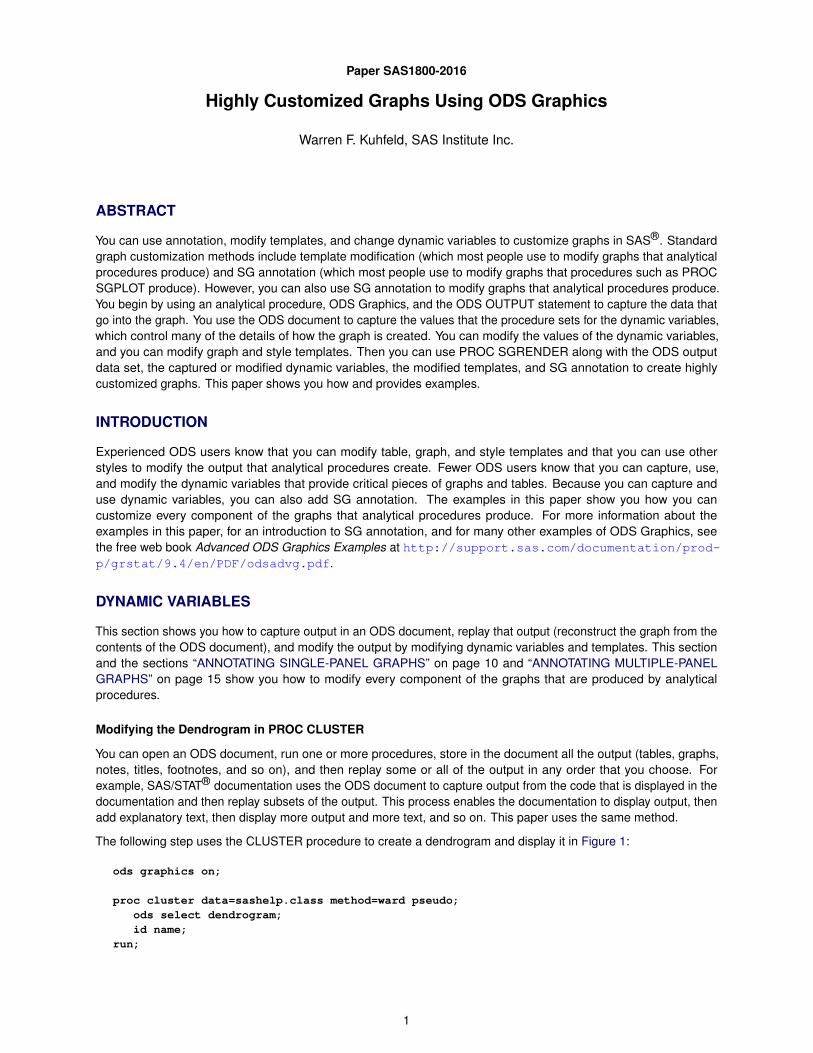
The following step uses the CLUSTER procedure to create a dendrogram and display it in Figure 1:

ods graphics on;

proc cluster data=sashelp.class method=ward pseudo;ods select dendrogram;id name;

run;

1

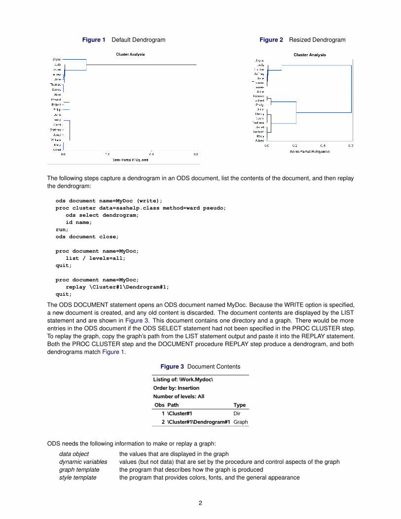
Figure 1 Default Dendrogram Figure 2 Resized Dendrogram

The following steps capture a dendrogram in an ODS document, list the contents of the document, and then replaythe dendrogram:

ods document name=MyDoc (write);proc cluster data=sashelp.class method=ward pseudo;

ods select dendrogram;id name;

run;ods document close;

proc document name=MyDoc;list / levels=all;

quit;

proc document name=MyDoc;replay \Cluster#1\Dendrogram#1;

quit;

The ODS DOCUMENT statement opens an ODS document named MyDoc. Because the WRITE option is specified,a new document is created, and any old content is discarded. The document contents are displayed by the LISTstatement and are shown in Figure 3. This document contains one directory and a graph. There would be moreentries in the ODS document if the ODS SELECT statement had not been specified in the PROC CLUSTER step.To replay the graph, copy the graph’s path from the LIST statement output and paste it into the REPLAY statement.Both the PROC CLUSTER step and the DOCUMENT procedure REPLAY step produce a dendrogram, and bothdendrograms match Figure 1.

Figure 3 Document Contents

Listing of: \Work.Mydoc\

Order by: Insertion

Number of levels: All

Obs Path Type

1 \Cluster#1 Dir

2 \Cluster#1\Dendrogram#1 Graph

ODS needs the following information to make or replay a graph:

data object the values that are displayed in the graphdynamic variables values (but not data) that are set by the procedure and control aspects of the graphgraph template the program that describes how the graph is producedstyle template the program that provides colors, fonts, and the general appearance

2

Both the data object and the dynamic variables are stored in the ODS document. Templates are stored in special filescalled item stores that SAS provides. You can display the dynamic variables for the dendrogram, store them in a SASdata set, and display the data set as follows:

proc document name=MyDoc;ods output dynamics=dynamics;obdynam \Cluster#1\Dendrogram#1;

quit;

proc print noobs data=dynamics;run;

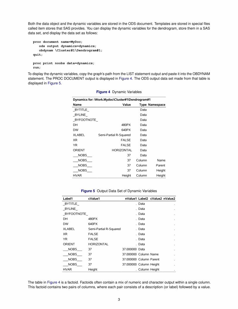
To display the dynamic variables, copy the graph’s path from the LIST statement output and paste it into the OBDYNAMstatement. The PROC DOCUMENT output is displayed in Figure 4. The ODS output data set made from that table isdisplayed in Figure 5.

Figure 4 Dynamic Variables

Dynamics for: \Work.Mydoc\Cluster#1\Dendrogram#1

Name Value Type Namespace

_BYTITLE_ Data

_BYLINE_ Data

_BYFOOTNOTE_ Data

DH 480PX Data

DW 640PX Data

XLABEL Semi-Partial R-Squared Data

XR FALSE Data

YR FALSE Data

ORIENT HORIZONTAL Data

___NOBS___ 37 Data

___NOBS___ 37 Column Name

___NOBS___ 37 Column Parent

___NOBS___ 37 Column Height

HVAR Height Column Height

Figure 5 Output Data Set of Dynamic Variables

Label1 cValue1 nValue1 Label2 cValue2 nValue2

_BYTITLE_ . Data .

_BYLINE_ . Data .

_BYFOOTNOTE_ . Data .

DH 480PX . Data .

DW 640PX . Data .

XLABEL Semi-Partial R-Squared . Data .

XR FALSE . Data .

YR FALSE . Data .

ORIENT HORIZONTAL . Data .

___NOBS___ 37 37.000000 Data .

___NOBS___ 37 37.000000 Column Name .

___NOBS___ 37 37.000000 Column Parent .

___NOBS___ 37 37.000000 Column Height .

HVAR Height . Column Height .

The table in Figure 4 is a factoid. Factoids often contain a mix of numeric and character output within a single column.This factoid contains two pairs of columns, where each pair consists of a description (or label) followed by a value.

3

The first pair of columns contains the name of each dynamic variable and its value, and the second pair containsthe type of the dynamic variable (specified in the data object or in the column) followed (when relevant) by the dataobject column name on which it was specified. Some dynamic variables exist in multiple parts of the data object. Thedynamic variable __NOBS__ (which is automatically created by ODS) exists in the overall data object and in multiplecolumns. Figure 4 shows that not all dynamic variables have been set to values. This is both common and reasonable.

The Name column in Figure 4 becomes the Label1 variable in the output data set displayed in Figure 5. TheValue column in Figure 4 becomes two output data set variables, cValue1 and nValue1. Similarly, the Type columnbecomes Label2 and the Namespace column becomes cValue2 and nValue2. The variables nValue1 and nValue2are numeric, and the variables cValue1 and cValue2 are character. Numeric values are captured in two forms: theactual numeric values are captured in the nValuen numeric variables, and formatted numeric values are captured inthe cValuen character variables. Character values are captured in the cValuen variables; the nValuen variableshave missing values for character variables.

You can replay the graph and explicitly specify that the values of the dynamic variables come from a data set (ratherthan from the dynamic variables that are stored in the ODS document):

proc document name=MyDoc;replay \Cluster#1\Dendrogram#1 / dynamdata=dynamics;

quit;

The REPLAY statement replays the graph. The DYNAMDATA= option names the data set that contains the dynamicvariables. The results again match Figure 1.

PROC CLUSTER determines the height and width of the dendrogram at run time after evaluating the number of rowsin the graph. These sizes are stored as dynamic variables. The dynamic variable DH sets the design height, and DWsets the design width. You can modify the values of the dynamic variables before you use them to replay the graph.The following steps recreate the dendrogram but by specifying smaller sizes:

data dynamics2;set dynamics;if label1 = 'DH' then cvalue1 = '400PX';if label1 = 'DW' then cvalue1 = '400PX';

run;

proc document name=MyDoc;replay \Cluster#1\Dendrogram#1 / dynamdata=dynamics2;

quit;

The results are displayed in Figure 2.

A few dynamic variable names are constant across templates and procedures. For example, the dynamic variables_BYTITLE_, _BYLINE_, and _BYFOOTNOTE_ are used to display BY lines in graphs when there are BY variables.ODS automatically creates the dynamic variable ___NOBS___ for each column. Most other dynamic variables are adhoc, although you might see patterns within procedures or graph types. You might need to look at the graph templateand at the GTL documentation to better understand the purpose of some dynamic variables.

You can find template names by specifying the following statement before running an analysis procedure:

ods trace on;

You can display the dendrogram template by copying its name from the SAS log and specifying it in a SOURCEstatement as follows:

proc template;source Stat.Cluster.Graphics.Dendrogram;

quit;

The results are displayed in Figure 6. You can see that the dynamic variables xr and yr are used to reverse axes, thevariable orient controls vertical and horizontal orientation, the variables xlabel and ylabel provide axis labels, andthe variable hvar provides the name of the cluster height column.

4

Figure 6 Dendrogram Template

define statgraph Stat.Cluster.Graphics.Dendrogram;

notes "Dendrogram";

dynamic dh dw orient xlabel ylabel hvar xr yr _byline_ _bytitle_

_byfootnote_;

begingraph / designheight=DH designwidth=DW;

entrytitle "Cluster Analysis";

layout overlay / xaxisopts=(label=XLABEL reverse=XR) yaxisopts=(label=

YLABEL reverse=YR discreteopts=(tickvaluefitpolicy=none));

dendrogram nodeid=NAME parentid=PARENT clusterheight=HVAR / orient=

ORIENT;

endlayout;

if (_BYTITLE_)

entrytitle _BYLINE_ / textattrs=GRAPHVALUETEXT;

else

if (_BYFOOTNOTE_)

entryfootnote halign=left _BYLINE_;

endif;

endif;

endgraph;

end;

You can modify both the template and the dynamic variables:

proc template;define statgraph Stat.Cluster.Graphics.Dendrogram;

notes "Dendrogram";dynamic dh dw orient xlabel ylabel hvar xr yr _byline_ _bytitle_

_byfootnote_;begingraph / designheight=DH designwidth=DW;

entrytitle "Cluster Analysis of the Class Data";layout overlay / xaxisopts=(label=' ' reverse=XR) yaxisopts=(label=

YLABEL reverse=YR discreteopts=(tickvaluefitpolicy=none));dendrogram nodeid=NAME parentid=PARENT clusterheight=HVAR /

orient=vertical;endlayout;if (_BYTITLE_)

entrytitle _BYLINE_ / textattrs=GRAPHVALUETEXT;else

if (_BYFOOTNOTE_)entryfootnote halign=left _BYLINE_;

endif;endif;

endgraph;end;

quit;

data dynamics2;set dynamics;if label1 = 'DH' then cvalue1 = '400PX';if label1 = 'DW' then cvalue1 = '600PX';

run;

proc document name=MyDoc;replay \Cluster#1\Dendrogram#1 / dynamdata=dynamics2;

quit;

5

Figure 7 Template and Dynamic Variable Modification Figure 8 Additional Style Modification

The PROC TEMPLATE step modifies the graph title, X-axis label, and the orientation of the graph. The results aredisplayed in Figure 7.

You can also change the ODS style:

ods listing style=analysis;proc document name=MyDoc;

replay \Cluster#1\Dendrogram#1 / dynamdata=dynamics2;quit;

This step changes the style for the LISTING destination to Analysis. For other destinations, you would substitute forLISTING. The results are displayed in Figure 8.

The preceding steps illustrate dynamic variable modification techniques that you can apply to other situations. However,you are not required to use them in this situation. The following step performs almost the same modification of thedendrogram:

proc cluster data=sashelp.class method=ward pseudoplots=dendrogram(vertical setheight=400 setwidth=600);

ods select dendrogram;id name;

run;

The results (except for the title) match Figure 8.

The following step restores the default style and deletes the modified graph template:

ods listing close;ods listing;proc template;

delete Stat.Cluster.Graphics.Dendrogram / store=sasuser.templat;run;

Modifying the Diagnostics Panel in PROC REG

This step runs PROC REG and captures the results in an ODS document:

ods graphics on;ods document name=MyDoc (write);proc reg data=sashelp.class;

model weight = height age / clb;quit;ods document close;

The diagnostics panel is displayed in Figure 9. The rest of this section modifies the table of statistics in the bottomright of the graph.

6

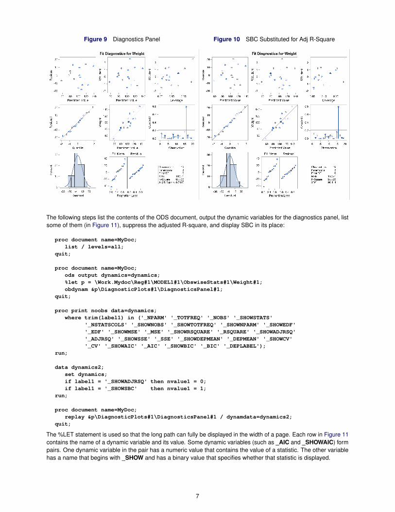
Figure 9 Diagnostics Panel Figure 10 SBC Substituted for Adj R-Square

The following steps list the contents of the ODS document, output the dynamic variables for the diagnostics panel, listsome of them (in Figure 11), suppress the adjusted R-square, and display SBC in its place:

proc document name=MyDoc;list / levels=all;

quit;

proc document name=MyDoc;ods output dynamics=dynamics;%let p = \Work.Mydoc\Reg#1\MODEL1#1\ObswiseStats#1\Weight#1;obdynam &p\DiagnosticPlots#1\DiagnosticsPanel#1;

quit;

proc print noobs data=dynamics;where trim(label1) in ('_NPARM' '_TOTFREQ' '_NOBS' '_SHOWSTATS'

'_NSTATSCOLS' '_SHOWNOBS' '_SHOWTOTFREQ' '_SHOWNPARM' '_SHOWEDF''_EDF' '_SHOWMSE' '_MSE' '_SHOWRSQUARE' '_RSQUARE' '_SHOWADJRSQ''_ADJRSQ' '_SHOWSSE' '_SSE' '_SHOWDEPMEAN' '_DEPMEAN' '_SHOWCV''_CV' '_SHOWAIC' '_AIC' '_SHOWBIC' '_BIC' '_DEPLABEL');

run;

data dynamics2;set dynamics;if label1 = '_SHOWADJRSQ' then nvalue1 = 0;if label1 = '_SHOWSBC' then nvalue1 = 1;

run;

proc document name=MyDoc;replay &p\DiagnosticPlots#1\DiagnosticsPanel#1 / dynamdata=dynamics2;

quit;

The %LET statement is used so that the long path can fully be displayed in the width of a page. Each row in Figure 11contains the name of a dynamic variable and its value. Some dynamic variables (such as _AIC and _SHOWAIC) formpairs. One dynamic variable in the pair has a numeric value that contains the value of a statistic. The other variablehas a name that begins with _SHOW and has a binary value that specifies whether that statistic is displayed.

7

The DATA step modifies two of the binary dynamic variables to suppress one statistic and display another. There is noneed to change the variable cValue1.

Figure 11 Dynamic Variables

Label1 cValue1 nValue1 Label2 cValue2 nValue2

_NPARM 3 3.000000 Data .

_TOTFREQ 19 19.000000 Data .

_NOBS 19 19.000000 Data .

_SHOWSTATS 1 1.000000 Data .

_NSTATSCOLS 2 2.000000 Data .

_SHOWNOBS 1 1.000000 Data .

_SHOWTOTFREQ 0 0 Data .

_SHOWNPARM 1 1.000000 Data .

_SHOWEDF 1 1.000000 Data .

_EDF 16 16.000000 Data .

_SHOWMSE 1 1.000000 Data .

_MSE 132.50623369 132.506234 Data .

_SHOWRSQUARE 1 1.000000 Data .

_RSQUARE 0.7729049378 0.772905 Data .

_SHOWADJRSQ 1 1.000000 Data .

_ADJRSQ 0.744518055 0.744518 Data .

_SHOWSSE 0 0 Data .

_SSE 2120.099739 2120.099739 Data .

_SHOWDEPMEAN 0 0 Data .

_DEPMEAN 100.02631579 100.026316 Data .

_SHOWCV 0 0 Data .

_CV 11.508106755 11.508107 Data .

_SHOWAIC 0 0 Data .

_AIC 95.580809248 95.580809 Data .

_SHOWBIC 0 0 Data .

_BIC 98.635496748 98.635497 Data .

_DEPLABEL Weight . Data .

The modified diagnostics panel is displayed in Figure 10. You will see SBC instead of adjusted R-square in thebottom right. This example illustrates dynamic-variable modification techniques that you can apply to other situations.However, you are not required to use them in this situation. The following step uses the STATS= option to perform thesame modification of the diagnostics panel:

proc reg data=sashelp.classplots=diagnostics(stats=(nobs nparm edf mse rsquare sbc));

model weight = height age / clb;quit;

The results match Figure 10.

Modifying Contour Plots in PROC KDE

The following steps create some random normal data, display them in a contour plot by using the KDE procedure,save the PROC KDE results in an ODS document, and replay the graph after modifying the values of the dynamicvariables that contain the variable names for the title:

8

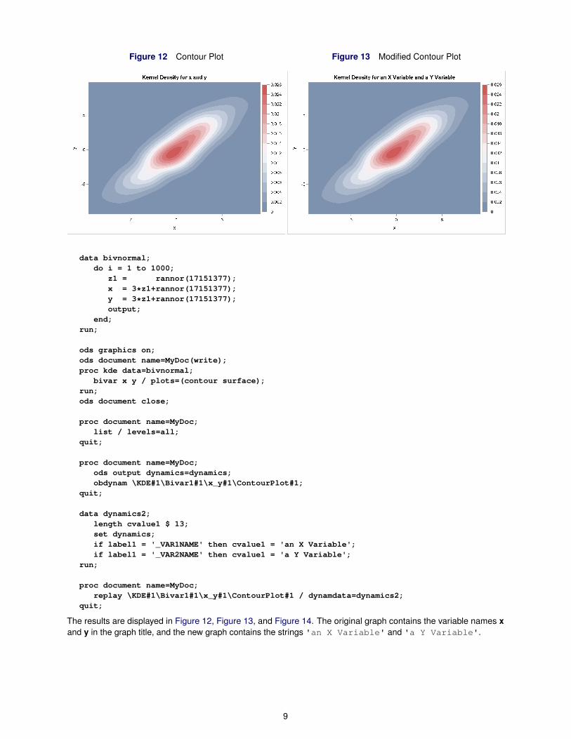
Figure 12 Contour Plot Figure 13 Modified Contour Plot

data bivnormal;do i = 1 to 1000;

z1 = rannor(17151377);x = 3*z1+rannor(17151377);y = 3*z1+rannor(17151377);output;

end;run;

ods graphics on;ods document name=MyDoc(write);proc kde data=bivnormal;

bivar x y / plots=(contour surface);run;ods document close;

proc document name=MyDoc;list / levels=all;

quit;

proc document name=MyDoc;ods output dynamics=dynamics;obdynam \KDE#1\Bivar1#1\x_y#1\ContourPlot#1;

quit;

data dynamics2;length cvalue1 $ 13;set dynamics;if label1 = '_VAR1NAME' then cvalue1 = 'an X Variable';if label1 = '_VAR2NAME' then cvalue1 = 'a Y Variable';

run;

proc document name=MyDoc;replay \KDE#1\Bivar1#1\x_y#1\ContourPlot#1 / dynamdata=dynamics2;

quit;

The results are displayed in Figure 12, Figure 13, and Figure 14. The original graph contains the variable names xand y in the graph title, and the new graph contains the strings 'an X Variable' and 'a Y Variable'.

9

Figure 14 ODS Document Contents and Dynamic Variables

Listing of: \Work.Mydoc\

Order by: Insertion

Number of levels: All

Obs Path Type

1 \KDE#1 Dir

2 \KDE#1\Bivar1#1 Dir

3 \KDE#1\Bivar1#1\x_y#1 Dir

4 \KDE#1\Bivar1#1\x_y#1\Inputs#1 Table

5 \KDE#1\Bivar1#1\x_y#1\Controls#1 Table

6 \KDE#1\Bivar1#1\x_y#1\ContourPlot#1 Graph

7 \KDE#1\Bivar1#1\x_y#1\SurfacePlot#1 Graph

Dynamics for:\Work.Mydoc\KDE#1\Bivar1#1\x_y#1\ContourPlot#1

Name Value Type Namespace

_BYTITLE_ Data

_BYLINE_ Data

_BYFOOTNOTE_ Data

_VAR1NAME "x" Data

_VAR2NAME "y" Data

___NOBS___ 3600 Data

___NOBS___ 3600 Column DensityX

___NOBS___ 3600 Column DensityY

___NOBS___ 3600 Column Density

ANNOTATING SINGLE-PANEL GRAPHS

Previous examples showed several ways to modify the graphs that SAS creates. This section builds on the section“DYNAMIC VARIABLES” on page 1, which shows you how to modify the dynamic variables and display the resultsby using PROC DOCUMENT. This section shows you how to capture dynamic variables, modify them, and create amodified graph by using PROC SGRENDER instead of PROC DOCUMENT. This approach enables you to use SGannotation to modify graphs that SAS analytical procedures create.

This step runs PROC REG, displays the diagnostics panel, and outputs the data object to a SAS data set:

ods graphics on;proc reg data=sashelp.class;

ods select diagnosticspanel;ods output diagnosticspanel=dp;model weight = height;

quit;

The results are displayed in Figure 15.

You might consider a naive approach to recreating the diagnostics panel from the data object and the graph templateby using PROC SGRENDER as follows:

proc sgrender data=dp template=Stat.REG.Graphics.DiagnosticsPanel;run;

For some graphs, this might completely work (if there are no dynamic variables) or it might completely fail (for example,if there is one graph statement and a critical part depends on dynamic variables). The preceding step partially works.In this example, the statistics table is completely missing, part of the title is missing, and some reference lines aremissing. The results are displayed in Figure 16.

You can run the following step to create the graph, output the data object to a SAS data set, and capture the dynamicvariables in an ODS document:

10

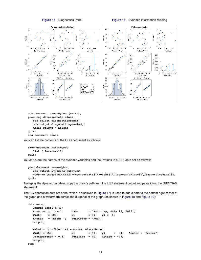
Figure 15 Diagnostics Panel Figure 16 Dynamic Information Missing

ods document name=MyDoc (write);proc reg data=sashelp.class;

ods select diagnosticspanel;ods output diagnosticspanel=dp;model weight = height;

quit;ods document close;

You can list the contents of the ODS document as follows:

proc document name=MyDoc;list / levels=all;

quit;

You can store the names of the dynamic variables and their values in a SAS data set as follows:

proc document name=MyDoc;ods output dynamics=outdynam;obdynam \Reg#1\MODEL1#1\ObswiseStats#1\Weight#1\DiagnosticPlots#1\DiagnosticsPanel#1;

quit;

To display the dynamic variables, copy the graph’s path from the LIST statement output and paste it into the OBDYNAMstatement.

The SG annotation data set anno (which is displayed in Figure 17) is used to add a date to the bottom right corner ofthe graph and a watermark across the diagonal of the graph (as shown in Figure 18 and Figure 19):

data anno;length Label $ 40;Function = 'Text'; Label = 'Saturday, July 25, 2015';Width = 100; x1 = 99; y1 = .1;Anchor = 'Right '; TextColor = 'Red';output;

Label = 'Confidential - Do Not Distribute';Width = 150; x1 = 50; y1 = 50; Anchor = 'Center';Transparency = 0.8; TextSize = 40; Rotate = -45;output;

run;

11

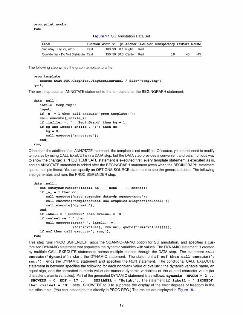
proc print noobs;run;

Figure 17 SG Annotation Data Set

Label Function Width x1 y1 Anchor TextColor Transparency TextSize Rotate

Saturday, July 25, 2015 Text 100 99 0.1 Right Red . . .

Confidential - Do Not Distribute Text 150 50 50.0 Center Red 0.8 40 -45

The following step writes the graph template to a file:

proc template;source Stat.REG.Graphics.DiagnosticsPanel / file='temp.tmp';

quit;

The next step adds an ANNOTATE statement to the template after the BEGINGRAPH statement:

data _null_;infile 'temp.tmp';input;if _n_ = 1 then call execute('proc template;');call execute(_infile_);if _infile_ =: ' BeginGraph' then bg + 1;if bg and index(_infile_, ';') then do;

bg = 0;call execute('annotate;');

end;run;

Other than the addition of an ANNOTATE statement, the template is not modified. Of course, you do not need to modifytemplates by using CALL EXECUTE in a DATA step, but the DATA step provides a convenient and parsimonious wayto show the change: a PROC TEMPLATE statement is executed first, every template statement is executed as is,and an ANNOTATE statement is added after the BEGINGRAPH statement (even when the BEGINGRAPH statementspans multiple lines). You can specify an OPTIONS SOURCE statement to see the generated code. The followingstep generates and runs the PROC SGRENDER step:

data _null_;set outdynam(where=(label1 ne '___NOBS___')) end=eof;if _n_ = 1 then do;

call execute('proc sgrender data=dp sganno=anno');call execute('template=Stat.REG.Graphics.DiagnosticsPanel;');call execute('dynamic');

end;if label1 = '_SHOWEDF' then cvalue1 = '0';if cvalue1 ne ' ' then

call execute(catx(' ', label1, '=',ifc(n(nvalue1), cvalue1, quote(trim(cvalue1)))));

if eof then call execute('; run;');run;

This step runs PROC SGRENDER, adds the SGANNO=ANNO option for SG annotation, and specifies a cus-tomized DYNAMIC statement that populates the dynamic variables with values. The DYNAMIC statement is createdby multiple CALL EXECUTE statements across multiple passes through the DATA step. The statement callexecute(’dynamic’); starts the DYNAMIC statement. The statement if eof then call execute(’;run;’); ends the DYNAMIC statement and specifies the RUN statement. The conditional CALL EXECUTEstatement in between specifies the following for each nonblank value of cvalue1: the dynamic variable name, anequal sign, and the formatted numeric value (for numeric dynamic variables) or the quoted character value (forcharacter dynamic variables). Part of the generated DYNAMIC statement is as follows: dynamic _NPARM = 2 ..._SHOWEDF = 0 _EDF = 17 ... _DEPLABEL = "Weight";. The statement if label1 = ’_SHOWEDF’then cvalue1 = ’0’; sets _SHOWEDF to 0 to suppress the display of the error degrees of freedom in thestatistics table. (You can instead do this directly in PROC REG.) The results are displayed in Figure 18.

12

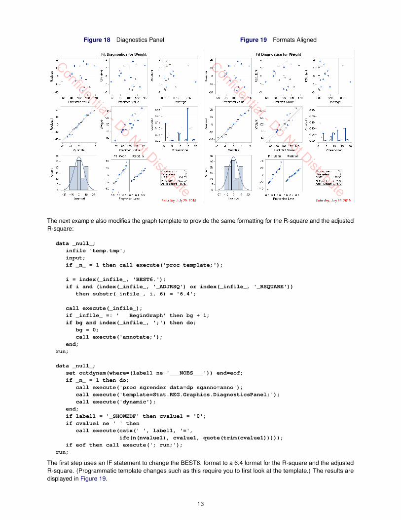
Figure 18 Diagnostics Panel Figure 19 Formats Aligned

The next example also modifies the graph template to provide the same formatting for the R-square and the adjustedR-square:

data _null_;infile 'temp.tmp';input;if _n_ = 1 then call execute('proc template;');

i = index(_infile_, 'BEST6.');if i and (index(_infile_, '_ADJRSQ') or index(_infile_, '_RSQUARE'))

then substr(_infile_, i, 6) = '6.4';

call execute(_infile_);if _infile_ =: ' BeginGraph' then bg + 1;if bg and index(_infile_, ';') then do;

bg = 0;call execute('annotate;');

end;run;

data _null_;set outdynam(where=(label1 ne '___NOBS___')) end=eof;if _n_ = 1 then do;

call execute('proc sgrender data=dp sganno=anno');call execute('template=Stat.REG.Graphics.DiagnosticsPanel;');call execute('dynamic');

end;if label1 = '_SHOWEDF' then cvalue1 = '0';if cvalue1 ne ' ' then

call execute(catx(' ', label1, '=',ifc(n(nvalue1), cvalue1, quote(trim(cvalue1)))));

if eof then call execute('; run;');run;

The first step uses an IF statement to change the BEST6. format to a 6.4 format for the R-square and the adjustedR-square. (Programmatic template changes such as this require you to first look at the template.) The results aredisplayed in Figure 19.

13

The following step deletes the modified template:

proc template;delete Stat.REG.Graphics.DiagnosticsPanel;

quit;

Assuming that you are creating exactly one graph and then annotating it, you can use the %ProcAnno macro in thefollowing steps to process the template and the dynamic variables:

ods graphics on;ods document name=MyDoc (write);proc reg data=sashelp.class;

ods select diagnosticspanel;ods output diagnosticspanel=dp;model weight = height;

quit;ods document close;

data anno;length Label $ 40;Function = 'Text'; Label = 'Saturday, July 25, 2015';Width = 100; x1 = 99; y1 = .1;Anchor = 'Right'; TextColor = 'Red';output;

Label = 'Confidential - Do Not Distribute';Width = 150; x1 = 50; y1 = 50; Anchor = 'Center';Transparency = 0.8; TextSize = 40; Rotate = -45;output;

run;

%macro procanno(data=, template=, anno=anno, document=mydoc);proc document name=&document;

ods exclude properties;ods output properties=__p(where=(type='Graph'));list / levels=all;

quit;

data _null_;set __p;call execute("proc document name=&document;");call execute("ods exclude dynamics;");call execute("ods output dynamics=__outdynam;");call execute(catx(' ', "obdynam", path, ';'));

run;

proc template;source &template / file='temp.tmp';

quit;

data _null_;infile 'temp.tmp';input;if _n_ = 1 then call execute('proc template;');call execute(_infile_);if _infile_ =: ' BeginGraph' then bg + 1;if bg and index(_infile_, ';') then do;

bg = 0;call execute('annotate;');

end;run;

14

data _null_;set __outdynam(where=(label1 ne '___NOBS___')) end=eof;if _n_ = 1 then do;

call execute("proc sgrender data=&data sganno=&anno");call execute("template=&template;");call execute('dynamic');

end;if cvalue1 ne ' ' then

call execute(catx(' ', label1, '=',ifc(n(nvalue1), cvalue1, quote(trim(cvalue1)))));

if eof then call execute('; run;');run;

proc template;delete &template;

quit;%mend;

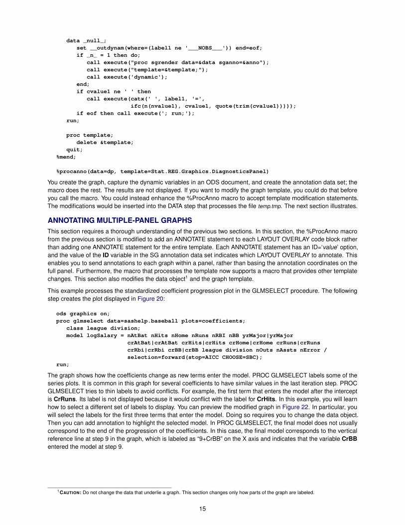
%procanno(data=dp, template=Stat.REG.Graphics.DiagnosticsPanel)

You create the graph, capture the dynamic variables in an ODS document, and create the annotation data set; themacro does the rest. The results are not displayed. If you want to modify the graph template, you could do that beforeyou call the macro. You could instead enhance the %ProcAnno macro to accept template modification statements.The modifications would be inserted into the DATA step that processes the file temp.tmp. The next section illustrates.

ANNOTATING MULTIPLE-PANEL GRAPHSThis section requires a thorough understanding of the previous two sections. In this section, the %ProcAnno macrofrom the previous section is modified to add an ANNOTATE statement to each LAYOUT OVERLAY code block ratherthan adding one ANNOTATE statement for the entire template. Each ANNOTATE statement has an ID=‘value’ option,and the value of the ID variable in the SG annotation data set indicates which LAYOUT OVERLAY to annotate. Thisenables you to send annotations to each graph within a panel, rather than basing the annotation coordinates on thefull panel. Furthermore, the macro that processes the template now supports a macro that provides other templatechanges. This section also modifies the data object1 and the graph template.

This example processes the standardized coefficient progression plot in the GLMSELECT procedure. The followingstep creates the plot displayed in Figure 20:

ods graphics on;proc glmselect data=sashelp.baseball plots=coefficients;

class league division;model logSalary = nAtBat nHits nHome nRuns nRBI nBB yrMajor|yrMajor

crAtBat|crAtBat crHits|crHits crHome|crHome crRuns|crRunscrRbi|crRbi crBB|crBB league division nOuts nAssts nError /selection=forward(stop=AICC CHOOSE=SBC);

run;

The graph shows how the coefficients change as new terms enter the model. PROC GLMSELECT labels some of theseries plots. It is common in this graph for several coefficients to have similar values in the last iteration step. PROCGLMSELECT tries to thin labels to avoid conflicts. For example, the first term that enters the model after the interceptis CrRuns. Its label is not displayed because it would conflict with the label for CrHits. In this example, you will learnhow to select a different set of labels to display. You can preview the modified graph in Figure 22. In particular, youwill select the labels for the first three terms that enter the model. Doing so requires you to change the data object.Then you can add annotation to highlight the selected model. In PROC GLMSELECT, the final model does not usuallycorrespond to the end of the progression of the coefficients. In this case, the final model corresponds to the verticalreference line at step 9 in the graph, which is labeled as “9+CrBB” on the X axis and indicates that the variable CrBBentered the model at step 9.

1CAUTION: Do not change the data that underlie a graph. This section changes only how parts of the graph are labeled.

15

Figure 20 Coefficient Progression

You begin by creating a data object and storing the graph along with the dynamic variables in an ODS document:

ods document name=MyDoc (write);proc glmselect data=sashelp.baseball plots=coefficients;

ods select CoefficientPanel;ods output CoefficientPanel=cp;class league division;model logSalary = nAtBat nHits nHome nRuns nRBI nBB yrMajor|yrMajor

crAtBat|crAtBat crHits|crHits crHome|crHome crRuns|crRunscrRbi|crRbi crBB|crBB league division nOuts nAssts nError /selection=forward(stop=AICC CHOOSE=SBC);

run;ods document close;

The next step reads the data object, extracts the parameter labels from steps 1 through 3 (by looking for the strings'1+', '2+', and '3+' in the variable StepLabel), and outputs the number of the last step to a macro variable_Step:

data labelthese(keep=par);set cp end=eof;retain f1-f3 1;if f1 and steplabel =: '1+' then do; f1 = 0; link s; end;if f2 and steplabel =: '2+' then do; f2 = 0; link s; end;if f3 and steplabel =: '3+' then do; f3 = 0; link s; end;if eof then call symputx('_step', step);return;

s: par = substr(steplabel, 3);output;return;

run;

proc print noobs;run;

The selected parameter labels are displayed in Figure 21.

16

Figure 21 First Three Terms

par

CrRuns

CrAtBat*CrAtBat

CrHits

The next step processes the data set that was created from the data object:

data cp2;set cp;match = 0;if step ne &_step then return;do i = 1 to ntolabel;

set labelthese point=i nobs=ntolabel;match + (par = parameter);end;

if not match then parameter = ' ';if nmiss(rhslabelYvalue) then rhslabelYvalue = StandardizedEst;

run;

The last part of the data set contains the coordinates and strings that are needed to label each profile. The DATAstep sets the parameter value to blank in the last step that PROC GLMSELECT considers (when the Step variablematches the _Step macro variable, which corresponds to the end of the profiles in the graph) for all but the first threeterms (that is, for all but those that match the labels stored in the data set Label). When the Y coordinate for a label ismissing (because PROC GLMSELECT suppressed it because of collisions), the Y coordinate value is restored.

The next step creates the %Tweak macro, which contains the code that modifies the graph template:

%macro tweak;if index(_infile_, 'datalabel=PARAMETER') then

_infile_ = tranwrd(_infile_, 'datalabel','markercharacterposition=right markercharacter');

if index(_infile_, 'curvelabel="Selected Step"') then_infile_ = tranwrd(_infile_, 'curvelabel="Selected Step"', ' ');

%mend;

The macro uses two IF statements, each of which performs a change:

� The first IF statement removes the DATALABEL= option in a SCATTERPLOT statement and instead specifies theMARKERCHARACTER= option. You can use the MARKERCHARACTER= option to position labels precisely ata point. In contrast, the DATALABEL= option moves labels that conflict. The first IF statement also adds theMARKERCHARACTERPOSITION=RIGHT option so that labels are positioned to the right of the coordinates.The TRANWRD (translate word) function performs the change, substituting a longer string from a shorter string.

� The second IF statement removes the “Selected Step” label for the reference line in the bottom panel. You willadd it back in through SG annotation.

The next step creates the annotation data set:

data anno;length ID $ 3 Function $ 9 Label $ 40;retain x1Space y1Space x2Space y2Space 'DataPercent' Direction 'In';length Anchor $ 10 xC1 xC2 $ 20;retain Scale 1e-12 Width 100 WidthUnit 'Data' CornerRadius 0.8

TextSize 7 TextWeight 'Bold'LineThickness 1.2 DiscreteOffset -0.3 LineColor 'Green';

ID = 'LO1'; Function = 'Text';Anchor = 'Right'; TextColor = 'Green';x1 = 55; y1 = 94;Label = 'Coefficients for the Selected Model'; output;

17

Function = 'Line'; x1 = .;x1Space = 'DataValue'; x2Space = x1Space;xc1 = '9+CrBB'; xc2 = '8+CrRuns*CrRuns';y1 = 94; y2 = 94; output;

Function = 'Rectangle'; y1Space = 'WallPercent';Anchor = 'BottomLeft'; y1 = 10;Height = 80; Width = 0.6; output;

ID = 'LO3'; Width = 100;Function = 'Text '; Label = 'Selected Value';x1Space = 'DataPercent'; y1Space = x1Space;Anchor = 'Left'; TextColor = 'Blue';x1 = 86; y1 = 84; output;

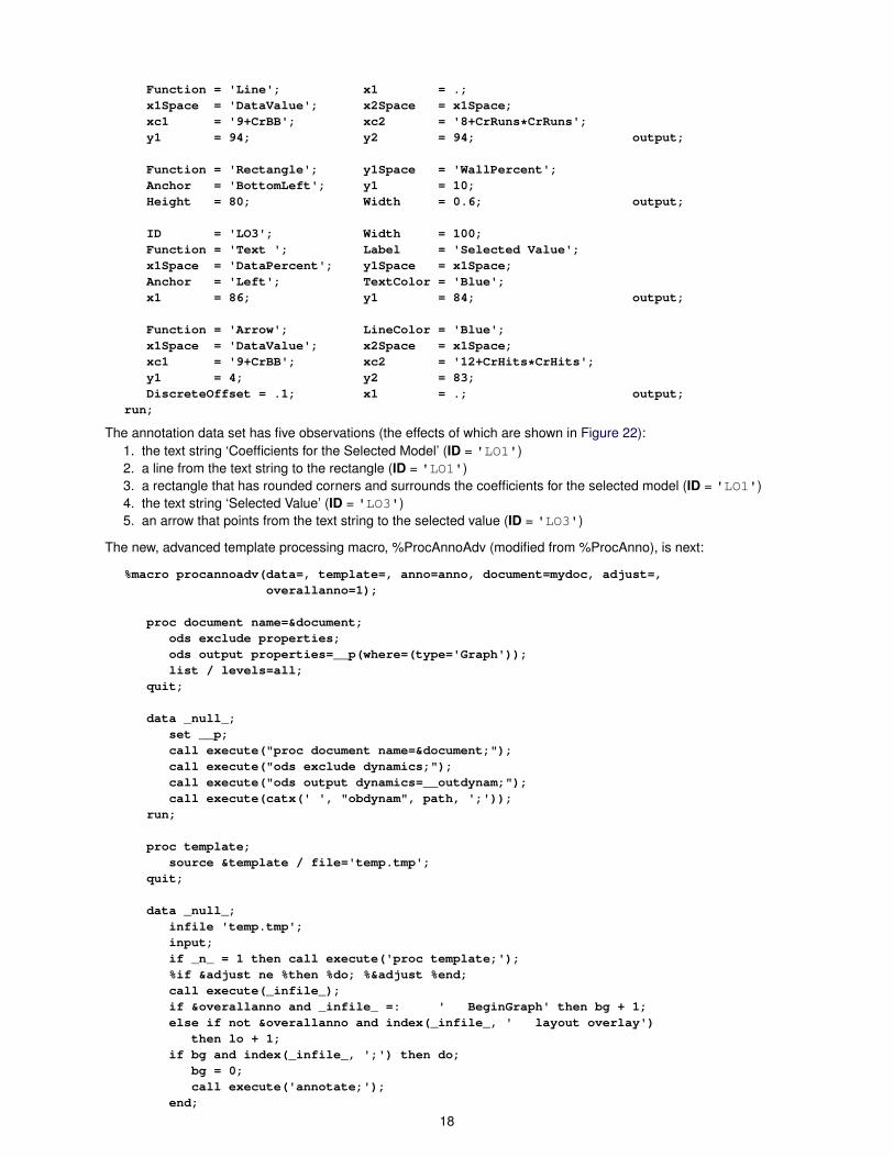
Function = 'Arrow'; LineColor = 'Blue';x1Space = 'DataValue'; x2Space = x1Space;xc1 = '9+CrBB'; xc2 = '12+CrHits*CrHits';y1 = 4; y2 = 83;DiscreteOffset = .1; x1 = .; output;

run;

The annotation data set has five observations (the effects of which are shown in Figure 22):1. the text string ‘Coefficients for the Selected Model’ (ID = 'LO1')2. a line from the text string to the rectangle (ID = 'LO1')3. a rectangle that has rounded corners and surrounds the coefficients for the selected model (ID = 'LO1')4. the text string ‘Selected Value’ (ID = 'LO3')5. an arrow that points from the text string to the selected value (ID = 'LO3')

The new, advanced template processing macro, %ProcAnnoAdv (modified from %ProcAnno), is next:

%macro procannoadv(data=, template=, anno=anno, document=mydoc, adjust=,overallanno=1);

proc document name=&document;ods exclude properties;ods output properties=__p(where=(type='Graph'));list / levels=all;

quit;

data _null_;set __p;call execute("proc document name=&document;");call execute("ods exclude dynamics;");call execute("ods output dynamics=__outdynam;");call execute(catx(' ', "obdynam", path, ';'));

run;

proc template;source &template / file='temp.tmp';

quit;

data _null_;infile 'temp.tmp';input;if _n_ = 1 then call execute('proc template;');%if &adjust ne %then %do; %&adjust %end;call execute(_infile_);if &overallanno and _infile_ =: ' BeginGraph' then bg + 1;else if not &overallanno and index(_infile_, ' layout overlay')

then lo + 1;if bg and index(_infile_, ';') then do;

bg = 0;call execute('annotate;');

end;

18

if lo and index(_infile_, ';') then do;lo = 0;lonum + 1;call execute(catt('annotate / id="LO', lonum, '";'));

end;run;

data _null_;set __outdynam(where=(label1 ne '___NOBS___')) end=eof;if _n_ = 1 then do;

call execute("proc sgrender data=&data");if symget('anno') ne ' ' then call execute("sganno=&anno");call execute("template=&template;");call execute('dynamic');

end;if cvalue1 ne ' ' then

call execute(catx(' ', label1, '=',ifc(n(nvalue1), cvalue1, quote(trim(cvalue1)))));

if eof then call execute('; run;');run;

proc template;delete &template;

quit;%mend;

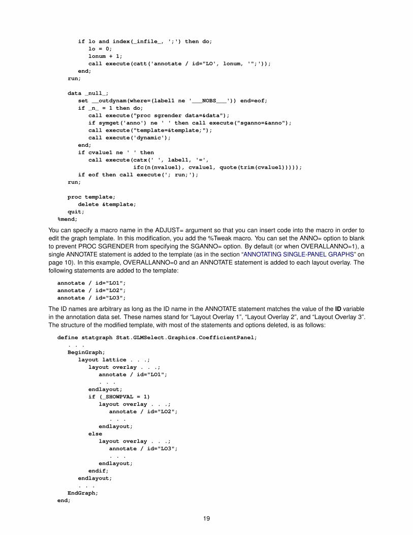
You can specify a macro name in the ADJUST= argument so that you can insert code into the macro in order toedit the graph template. In this modification, you add the %Tweak macro. You can set the ANNO= option to blankto prevent PROC SGRENDER from specifying the SGANNO= option. By default (or when OVERALLANNO=1), asingle ANNOTATE statement is added to the template (as in the section “ANNOTATING SINGLE-PANEL GRAPHS” onpage 10). In this example, OVERALLANNO=0 and an ANNOTATE statement is added to each layout overlay. Thefollowing statements are added to the template:

annotate / id="LO1";annotate / id="LO2";annotate / id="LO3";

The ID names are arbitrary as long as the ID name in the ANNOTATE statement matches the value of the ID variablein the annotation data set. These names stand for “Layout Overlay 1”, “Layout Overlay 2”, and “Layout Overlay 3”.The structure of the modified template, with most of the statements and options deleted, is as follows:

define statgraph Stat.GLMSelect.Graphics.CoefficientPanel;. . .BeginGraph;

layout lattice . . .;layout overlay . . .;

annotate / id="LO1";. . .

endlayout;if (_SHOWPVAL = 1)

layout overlay . . .;annotate / id="LO2";. . .

endlayout;else

layout overlay . . .;annotate / id="LO3";. . .

endlayout;endif;

endlayout;. . .

EndGraph;end;

19

You can use the three IDs in order to modify each of the three overlays. In this template, the first LAYOUT OVERLAYis unconditionally used and either the second and or third LAYOUT OVERLAY is conditionally used (because of the IFand ELSE statements). In this example, the first and third LAYOUT OVERLAYs are used.

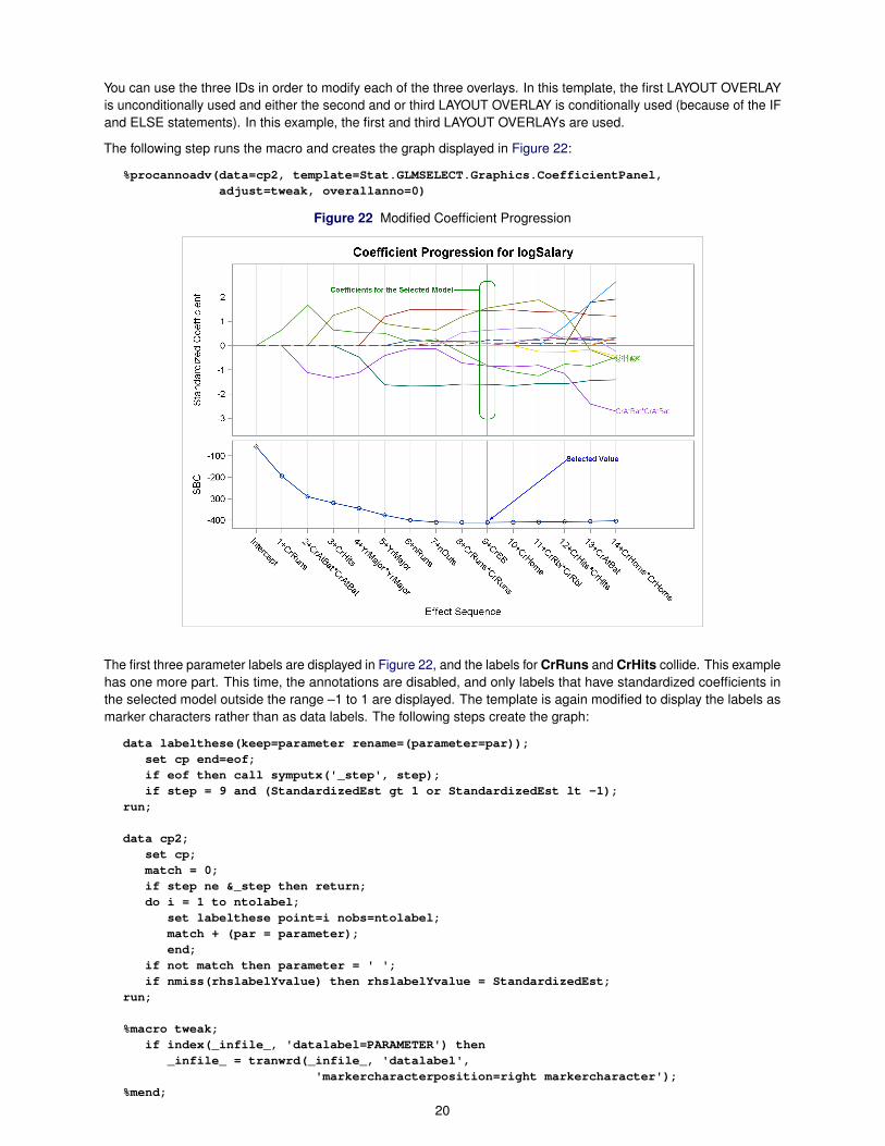
The following step runs the macro and creates the graph displayed in Figure 22:

%procannoadv(data=cp2, template=Stat.GLMSELECT.Graphics.CoefficientPanel,adjust=tweak, overallanno=0)

Figure 22 Modified Coefficient Progression

The first three parameter labels are displayed in Figure 22, and the labels for CrRuns and CrHits collide. This examplehas one more part. This time, the annotations are disabled, and only labels that have standardized coefficients inthe selected model outside the range –1 to 1 are displayed. The template is again modified to display the labels asmarker characters rather than as data labels. The following steps create the graph:

data labelthese(keep=parameter rename=(parameter=par));set cp end=eof;if eof then call symputx('_step', step);if step = 9 and (StandardizedEst gt 1 or StandardizedEst lt -1);

run;

data cp2;set cp;match = 0;if step ne &_step then return;do i = 1 to ntolabel;

set labelthese point=i nobs=ntolabel;match + (par = parameter);end;

if not match then parameter = ' ';if nmiss(rhslabelYvalue) then rhslabelYvalue = StandardizedEst;

run;

%macro tweak;if index(_infile_, 'datalabel=PARAMETER') then

_infile_ = tranwrd(_infile_, 'datalabel','markercharacterposition=right markercharacter');

%mend;

20

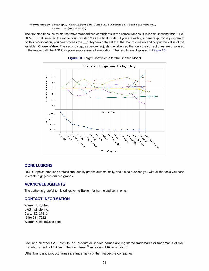
%procannoadv(data=cp2, template=Stat.GLMSELECT.Graphics.CoefficientPanel,anno=, adjust=tweak)

The first step finds the terms that have standardized coefficients in the correct ranges; it relies on knowing that PROCGLMSELECT selected the model found in step 9 as the final model. If you are writing a general-purpose program todo this modification, you can process the __outdynam data set that the macro creates and output the value of thevariable _ChosenValue. The second step, as before, adjusts the labels so that only the correct ones are displayed.In the macro call, the ANNO= option suppresses all annotation. The results are displayed in Figure 23.

Figure 23 Larger Coefficients for the Chosen Model

CONCLUSIONS

ODS Graphics produces professional-quality graphs automatically, and it also provides you with all the tools you needto create highly customized graphs.

ACKNOWLEDGMENTS

The author is grateful to his editor, Anne Baxter, for her helpful comments.

CONTACT INFORMATION

Warren F. KuhfeldSAS Institute Inc.Cary, NC, 27513(919) 531-7922Warren.Kuhfeld@sas.com

SAS and all other SAS Institute Inc. product or service names are registered trademarks or trademarks of SASInstitute Inc. in the USA and other countries. ® indicates USA registration.

Other brand and product names are trademarks of their respective companies.

21