Highway Effects on Vehicle PerformanceFHWA-RD-00-164 JANUARY 2001

Research, Development, and TechnologyTurner-Fairbank Highway Research Center6300 Georgetown PikeMcLean, VA 22101-2296

FOREWORD

This report presents an overview of the efforts to develop a convenient procedure to simulate operation of motor vehicles on highways of an arbitrary configuration and to estimate fuel consumption and exhaust emissions resulting from reasonable operations of those vehicles.

Highway pavements, grades, curves, and wind and traffic flow rates affect the fuel consumption and air contaminant emission rates for a given section of highway or a network of highways. Vehicles were tested on a large-roll dynamometer and under various road and traffic flow conditions. Evaluations of other analytical and experimental results were also made. Based on experiments and evaluations, clear relationships were developed relating specific loads and speeds to pollutant emissions and fuel consumption rates. These data were used to develop a user-friendly personal computer program called the Vehicle/ Highway Performance Predictor Algorithm. This model is intended to receive any reasonable mix of data for a selection of various vehicles that may approximate the traffic mix for given locations for past, current, and reasonable future years. The procedure can be used by highway planners and designers, environmental engineers, and traffic engineers, particularly those involved in Intelligent Transportation Systems, to evaluate local microspace air quality evaluations or larger area air pollution emission rates to determine impacts and conformity to the State Implementation Plans for the areas. This model is intended to use modal emissions and fuel usage rates that are based on various speeds and loads of vehicles in operation.

This report reviews the principles involved in determining the external loads on vehicles from longitudinal and lateral accelerations, aerodynamic drag, rolling resistance, and various grades. Examples of loads measured in the field and related dynamometer tests for selected vehicles for fuel consumption and air contaminant emissions are provided.

Detailed data have not been archived. However, informal interim reports containing added experimental information are available from the Federal Highway Administration Offices of Natural Environment, Infrastructure Research and Development, Traffic Operations Research and Development, and four Federal Highway Administration Resource Centers.

T. Paul Teng Director, Office of Infrastructure Research and Development, P.E.

NOTICE

This document is disseminated under the sponsorship of the Department of Transportation in the interest of information exchange. The United States Government assumes no liability for its contents or use thereof. This report does not constitute a standard, specification, or regulation. The United States Government does not endorse products or manufacturers. Trade or manufacturers' names appear herein solely because they are considered essential to the object of this document.

r--.- -

Technical Report Documentation Page

1. Report No. FHWA-RD-00-164

2. Government Accession No. 3. Recipient’s Catalog No.

4. Title and Subtitle HIGHWAY EFFECTS ON VEHICLE PERFORMANCE

5. Report Date

7. Author(s) 6. Performing Organization Code Earl C. Klaubert HW X114/ H1005/ 3Kl

9. Performing Organization Name and Address 8. Performing Organization Report No.

U.S. Department of Transportation Research and Special Programs Administration John A. Volpe National Transportation Systems Center Cambridge, MA 02142

DOT-VNTSC-FHWA -1HW14

12. Sponsoring Agency Name and Address

U.S. Department of Transportation Federal Highway Administration Offices of Infrastructure Research and Development and Oftice of Environment and Planning McLean, VA 22101-2296 and Washington, DC 20590, respectively

10. Work Unit No. (TRAIS)

11. Contract / Grant. xppalrl-GWA

13. Type of Report and Period Covered Final Report 1978-2001

14. Sponsoring Agency Code

15. Supplementary Notes FHWA Program Manager: Howard A. Jongedyk HRDI-09, FHWA Contact: Richard A. Schoeneberg, HEPN -1, Office of Natural Environment; ADAC Corp., Woburn, MA, 02154; Digital Equipment Corp., Waltham, MA. 02154; ACUREX Corp., Mountainview CA, 94042; Astech Electronics, LTD, Farnham, Surrey GU9 7LP, England #ll GWA Xppa -GWA X-year

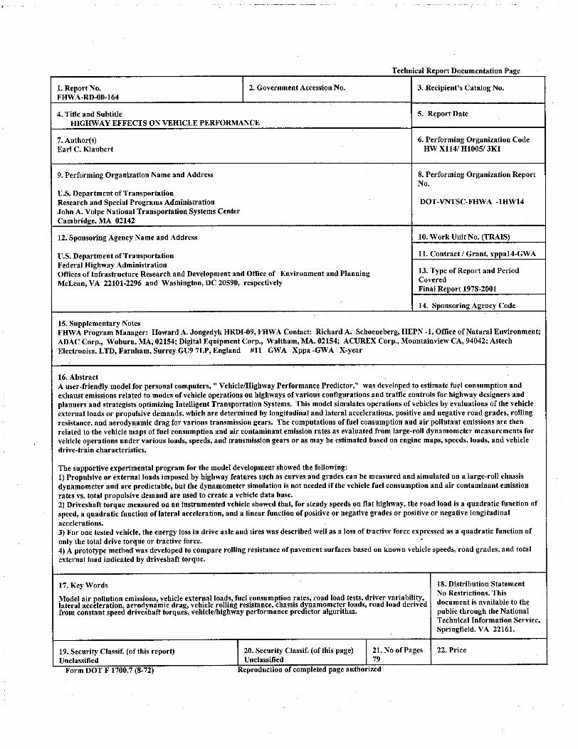
16. Abstract A user-friendly model for personal computers, ” Vehicle/Highway Performance Predictor,” was developed to estimate fuel consumption and exhaust emissions related to modesof vehicle operations on highways of various configurations and traffic controls for highway designers and planners and strategists optimizing Intelligent Transportation Systems. This model simulates operations of vehicles by evaluations of the vehicle external loads or propulsive demands, which are determined by longitudinal and lateral accelerations, positive and negative road grades, rolling resistance, and aerodynamic drag for various transmission gears. The computations of fuel consumption and air pollutant emissions are then related to the vehicle maps of fuel consumption and air contaminant emission rates as evaluated from large-roll dynamometer measurements for vehicle operations under various loads, speeds, and transmission gears or as may be estimated based on engine maps, speeds, loads, and vehicle drive-train characteristics.

The supportive experimental program for the model development showed the following: 1) Propulsive or external loads imposed by highway features such as curves and grades can be measured and simulated on a large-roll chassis dynamometer and are predictable, but the dynamometer simulation is not needed if the vehicle fuel consumption and air contaminant emission rates vs. total propulsive demand are used to create a vehicle data base. 2) Driveshaft torque measured on an instrumented vehicle showed that, for steady speeds on flat highway, the road’load is a quadratic function of speed, a quadratic function of lateral acceleration, and a linear function of positive or negative grades or positive or negative longitudinal accelerations. 3) For one tested vehicle, the energy loss in drive axle and tires was described well as a loss of tractive force expressed as a quadratic function of only the total drive torque or tractive force. .

4) A prototype method was developed to compare rolling resistance of pavement surfaces based on known vehicle speeds, road grades, and total external load indicated by driveshaft torque.

17. Key Words 18. Distribution Statement

Model air pollution emissions, vehicle external loads, fuel consumption rates, road load tests, driver variability, No Restrictions. This

lateral acceleration, aerodynamic drag, vehicle rolling resistance, chassis dynamometer loads, road load dertved document is avai1able to the from constant speed driveshaft torques, vehicle/highway performance predictor algorithm. public through the National

Technical Information Service, Springfield, VA 22161.

19. Security Classif. (of this report) Unclassified

Form DOT F 1700.7 (8-72)

20. Security Classif. (of this page) 21. No of Pages Unclassified 79

Reproduction of completed page authorized

22. Price

APPROXIMATE CONVERSIONS FROM SI UNITS APPROXIMATE CONVERSIONS TO SI UNITS Symbol When You Know Multlply By To Find Symbol

in ft Yd mi

inches feet YdS miles

LENGTH 25.4 0.305 0.914 1.61

AREA

millimeters meters meters kilometers

m

L

mm m

L

millimeters meters meters kilometers

LENGTH 0.039 3.26 1.09 0.621

AREA

in* fF Yd” ac mP

square inches square feet square yards acres square miles

645.2 0.093 0.836 0.405 2.59

VOLUME

square millimeters square meters square meters hectares square kilometers

m* m2 ha km*

mm* m*

,m* ha km*

square millimeters 0.0016 square inches: in2 square meters 10.764 square feet fF square meters 1.195 square yards Y@ hectares 2.47 acres ac square kilometers 0.386 square miles mi*

VOLUME

fl 02 fluid ounces 29.57 milliliters

r’ gallons 3.765 liters cubic feet 0.026 cubic meters

Y@ cubic yards 0.765 cubic meters

NOTE: Volumes greater than loo0 I shall be shown in m3.

mL mL milliliters 0.034 fluid ounces fl oz L L liters 0.264 gallons gal ma m3 cubic meters 35.71 cubic feet fP m3 m3 cubic meters 1.307 cubic yards Y@

MASS MASS

02

lb T

ounces 26.35 grams pounds .0.454 short tons (2000 lb) 0.907

kilograms megagrams (oi “metric ton”)

TEMPERATURE (exact)

9 kg

ysr,

grams 0.035 ounces OZ kilograms 2.202 pounds lb megagrams 1.103 short tons (2000 lb) T (or “metric ton”)

TEMPERATURE (exact)

“F Fahrenheit 5( F-32)/9 Celcius temperature or (F-32)/1.6 temperature

ILLUMINATION

“C Celcius temperature

1.8C +32

ILLUMINATION

fc fl

foot-candfes 10.76 lux foot-Lamberts 3.426 candela/m*

FORCE and PRESSURE or STRESS

IX

c&m* lux 0.0929 foot-candies candela/m2 0.2919 foot-Lamberts

FORCE and PRESSURE or STRESS

Ibf lbf/in?

poundforce poundforce per square inch

4.45 newtons N N newtons 0.225 6.69 kilopascals kPa kPa kilopascals 0.145

Symbol When You Know Multiply By To Find Symbol

inches in feet ft yards Yd miles mi

Fahrenheit temperature

poundforce poundforce Per square inch )

fc fl

Ibf Ibf/in*

SI is the symbol for the International System of Units. Appropriate rounding should be made to comply with Section 4 of ASTM E380.

(Revised September 1993)

PREFACE

A user-friendly model for personal computers, “Vehicle/Highway Performance Predictor”(HPP), was developed for highway designers and planners and strategists to estimate fuel consumption and exhaust emissions related to modes of vehicle operations on highways of various configurations and traffic controls, e.g. the optimization of Intelligent Transportation Systems with considerations for fuel consumption and air pollution impacts. This model simulates operations of vehicles by evaluating the vehicle external loads or propulsive demands determined by longitudinal and lateral accelerations, positive and negative road grades, rolling resistance, and aerodynamic drag for various transmission gears. The resultant computations of fuel consumption and air pollutant emissions are then related to the vehicle maps of fuel consumption and air contaminant emission rates as evaluated from large-roll dynamometer measurements for vehicle operations under various loads, speeds, and transmission gears or as may be estimated based on engine maps, speeds, loads, and vehicle drive-train characteristics.

The supportive experimental program for the model development showed that:

1) Propulsive or external loads imposed by highway features such as curves and grades can be measured and simulated on a large-roll chassis dynamometer and are predictable, but the dynamometer simulation is not needed if the vehicle fuel consumption and air contaminant emission rates vs. total propulsive demand are used to create a vehicle data base.

2) Driveshaft torque measured on an instrumented vehicle showed that, for steady speeds on a flat highway, the road load is a quadratic function of speed, a quadratic function of lateral acceleration, and a linear function of positive or negative grades or positive or negative longitudinal accelerations.

3) For one tested vehicle, the energy loss in the drive axle and tires was described well as a loss of tractive force expressed as a quadratic function of only the total drive torque or tractive force.

4) A prototype method of comparing rolling resistance of pavement surfaces based on known vehicle speeds, road grades, road curves, and total external load indicated by driveshaft torque could be developed.

. . . 111

Section

1.0 PROJECTDEFINITION ................................................................. 1 1.1 PROJECTOBJECTIVES ........................................................ 1 1.2 HIGHWAY FACTORS AFFECTING FUEL ECONOMY ............................. 1 1.3 PROJECT REQUIREMENTS ..................................................... 2

2.0 APPROACH......................................................................~.... 5

3.0 MAJOR ACCOMPLISHMENTS AND EXPERIMENTAL RESULTS . . . . . . . . . . . . . . . . . . . . . . . . . 7

3.1

3.2 3.3 3.4 3.5

3.6 3.7

3.8 3.9

3.10

3.11

COMPUTER PROGRAM FOR PREDICTION OF VEHICLE PERFORMANCE ONHIGHWAYS . . . . . . . . . . . . . . . . . . . . . . . . . . . . . . . . . . . . . . . . . . . . . . . . . . . . . . . . . . . 7

EFFECTOFROADGRADE . . . . . . . . . . . . . . . . . . . . . . . . . . . . . . . . . . . . . . . . . . . . . . . . . . . . . 7 EFFECT OF HORIZONTAL CURVATURE . . . . . . . . . . . . . . . . . . . . . . . . . . . . . . . . . . . . . . . . 8 DETERMINATION OF ROAD LOAD FROM CONSTANT-SPEED TORQUES. . . . . . . . . . 9 PAVEMENT FRICTION COMPARISON WITH TORQUE-INSTRUMENTED

VEHICLE . . . . . . . . . . . . . . . . . . . . . . . . . . . . . . . . . . . . . . . . . . . . . . . . . . . . . . . . . . . . . 10 INFLUENCE OF DRIVER VARIANCE ON HIGHWAY FUEL ECONOMY . . . . . . . . . . . . 10 EFFECT OF TRACTIVE FORCE LEVEL ON ENERGY DISSIPATION IN TIRESANDAXLE............................................................. 11 EXPERIMENTAL VEHICLE DATA BASES . . . . . : . . . . . . . . . . . . . . . . . . . . . . . . . . . . . . . . . 11 SYNTHESIS OF FUEL ECONOMY (AND AIR CONTAMINANT EMISSION) DATA FOR VEHICLES NOT TESTED . . . . . . . . . . . . . . . . ., . . . . . . . . . . . . . . . . . . . . . . . . . . 12 FRICTION MEASUREMENTS BEFORE AND AFTER RESURFACING A HIGHWAY . . . . . . . . . . . . . . . . . . . . . . . . . . . . . . . . . . . . . . . . . . . . . . . . . . . . . . . . . . . . . . . . . 12 FUEL CONSUMPTION DURING ACCELS AND DECELS ON CHASSIS

DYNAMOMETER . . . . . . . . . . . . . . . . . . . . . . . . . . . . . . . . . . . . . . . . . . . . . . . . . . . . . . . . . 13

4.0 CONCLUSIONS...............................................................15

4.1 EFFECTS OF HIGHWAY GEOMETRIC FEATURES ON VEHICLE PE~ORMANCE.......................................................... 15

4.2 VEHICLE/HIGHWAY PERFORMANCE PREDICTOR (HPP) SIMULATION . . . . . . . . . . . . . . . . . . . . . . . . . . . . . . . . . . . . . . . . . . . . . . . . . . . . . 15

APPENDIX A: THE VEHICLE/HIGHWAY PERFORMANCE PREDICTOR (HPP) ALGORITHM . . . . . . . . . . . . . . . . . . . . . . . . . . . . . . . . . . . . . . . . . . . . . . . . . . . . . . . . . . . . . . . . 17

A.1 DESCRIPTION OF OPERATION, PROTOTYPE VERSION ........................... 17 A. 1.1 UNIT OPERATIONS ON ONE ROAD ELEMENT FOR ONE VEHICLE ........... 17

A.l.l.l RoadElements.. ..................................................... 17 A.1.1.2 Speed ............................................................. 20 A.1.1.3 RoadLoad ......................................................... 20 A.1.1.5 Grade ........................................................... ..2 0 A.1.1.6 Curvature ................................... . ....................... 21

iv

TABLE OF CONTENTS (CONTINUED)

Section

A. 1.1.7 Driveshaft Torque . . . . . . . . . . . . . . . . . . . . . . . . . A. 1.1.8 Fuel Consumption . . . . . . . . . . . . . . . . . . . . . . . . . A. I. 1.9 Performance Limits . . . . . . . . . . . . . . . . . . . . . . . .

A. 1.2 SUMMATIONS OVER ENTIRE ROAD LENGTH . . . A.1.3 HIGHWAY GEOMETRY PROCESSOR (HGP) . . . . . . A. 1.4 COMPUTERIZATION OF ALGORITHM . . . . . . . . . .

A.1.4.1 Rationale . . . . . . . . . . . . . . . . . . . . . . . . . . . . . . . . A. 1.4.2 Implementation . . . . . . . . . . . . . . . . . . . . . . . . . . .

A. 1.5 OVERVIEW OF COMPLETE HPP SOFTWARE . . . . .

.........

.........

.........

.........

.........

.........

.........

.........

. . . . . .

......

......

......

......

......

......

......

......

Pap;e

........ 21

........ 22

........ 22

........ 22

........ 23

........ 23

........ 23

........ 23

........ 24

A.2 INPUT DATA REQUIRED PRESENTLY ............................................ 28 A.2.1 HIGHWAY GRADE VS. DISTANCE (USER INPUT) ........................... 28 A.2.2 HIGHWAY CURVATURE VS. DISTANCE (USER INPUT) ..................... 28 A.2.3 SPEED VS. DISTANCE/IDLE VS. TIME (USER INPUT) ........................ 29 A.2.4 REPORT STATIONS FOR INTERMEDIATE OUTPUTS (USER INPUT) ........... 29 A.2.5 VEHICLE DATA (FOR HPP) .............................................. 30

A.3 OPTIONS FOR FUTURE EXPANSION ............................................. 30

APPENDIX B: PROTOTYPE VEHICLE/HIGHWAY PERFORMANCE PREDICTOR ALGORITHM . . . . . . . . . . . . . . . . . . . . . . . . . . . . . . . . . . . . . . . . . . . . . . . . . . . . . . . . . . . . . . . . . . . . . . . 31

APPENDIX C : EMPIRICAL TEST DATA 1. . . . . . . . . . . . . . . . . . . . . . . . . . . . . . . . . . . . . . . . . . . . . . . . . 35

Cl EMPIRICAL DATA: DEVELOPMENT FOR ONE VEHICLE ......................... C. 1.1 ROAD LOAD VS. SPEED FROM RUNWAY TESTS-CITATION ............... C. 1.2 TORQUE INCREMENT ON CURVES-CITATION ........................... C. 1.3 NORMALIZED TORQUE INCREMENT ON CURVES-CITATION ............. C. 1.4 FUEL ECONOMY VS. TORQUE, SPEED, AND GEAR-CITATION ....... 1 .... C. 1.5 TRACTIVE FORCE LOSS IN DRIVE AXLE AND TIRES-PONTIAC ...........

C.2 EMPIRICAL DATA: COMPARATIVE DATA ON THREE CARS . . . . . . . . . . . . . . . . . . . . . . C.2.1 DERIVED TRACTIVE FORCE FOR THREE VEHICLES . . . . . . . . . . . . . . . . . . . I . . C.2.2 NORMALIZED CURVE-TORQUE INCREMENT FOR THREE CARS . . . . . . . . . . . . C.2.3 FUEL ECONOMY DATA FOR TWO ADDITIONAL VEHICLES . . . . . . . . . . . . . . .

35 35 37 39 41 44

44 44 47 50

APPENDIX D : TEST FACILITIES AND PROCEDURES . . . . . . . . . . . . . . . . . . . . . . . . . . . . . . . . . . . . . . 59

D.1 ROADTESTFACILITIES ......................................................... 59 D.l.l QUABBIN RESERVOIR .................................................. 59 D. 1.2 SOUTH WEYMOUTH NAVAL AIR STATION ............................... 59 D. 1.3 QUONSET POINT NAVAL AIR STATION .................................. 59 D.1.4 BANGOR INTERNATIONAL AIRPORT .................................... 60

V

%‘AliiLtE OF CONTENTS (CONTINUED)

Section

D.2 VEHICLE TEST AND DATA ANALYSIS PROCEDURES .............................. 60

D.2.1 PILOTTESTSONROAD .................................... w... ......... 60 D.2.1.1 Test Procedure ...................................................... 60

D.2.1.2 Data Analysis ....................................... .1 ............. 61 D.2.2 VEHICLE ROAD LOAD VS. SPEED ........................................ 62

D.2.2.1 TestProcedure ............................................... ..6 2 D.2.2.2 Data Analysis .................................................. 63

D.2.3 HORIZONTAL CURVATURE EFFECT ..................................... 64 D.2.3.1 TestProcedure.. ............................................. ..:6 4 D.2.3.2 DataAnalysis................................................: . 65

D.2.4 CHASSIS DYNAMOMETER TESTS ........................................ 66 D.2.4.1 Test Point Determination .......................................... 67 D.2.4.2 Performance Mapping ............................................ 68

D.2.4.3 DataAnalysis ................................................... 69

REFERENCES ........................................................................... 71

Vi

LIST OF FIGURES

Figure PaJg

1.

2.

3.

4.

5.

6.

7.

8.

9.

10.

11.

12.

13.

14.

15.

Example of speed and elapsed time vs. distance . . . . . . . . . . . . . . . . . . . . . . . . . . . . . . . . . . . . . . . . . . . 19

Vehicle/highway performance predictor software-logic diagram. . . . . . . . . . . . . . . . . . . . . . . . . . . . . . . 25

Citation road load torque vs. speed. . . . . . . . . . . . . . . . . . . . . . . . . . . . . . . . . . . . . . . . . . . . . . . . . . . . . . 36

Total torque and torque increment on plane curves . . . . . . . . . . . . . . . . . . . . . . . . . . . . . . . . . . . . . . . . . 3 8

Normalized curve-torque increment vs. lateral acceleration . . . . . . . . . . . . . . . . . . . . . . . . . . . . . . . . . . 40

Citation fuel economy vs. driveshaft torque and gear . . . . . . . . . . . . . . . . . . . . . . . . . . . . . . . . . . . . . . . 43

Tractive force loss vs. total force . . . . . . . . . . . . . . . . . . . . . . . . . . . . . . . . . . . . . . . . . . . . . . . . . . . . . . . 45

Road load derived tractive force vs. speed - three cars . . . . . . . . . . . . . . . . . . . . . . . . . . . . . . . . . . . . . . 48

Normalized curve-torque increment - three cars . . . . . . . . . . . . . . . . . . . . . . . . . . . . . . . . . . . . . . . . . . . 49

Composite normalized curve-torque increment - three cars . . . . . . . . . . . . . . . . . . . . . . . . . . . . . . . . . . . 5 1

Chevette fuel economy vs. driveshaft torque, fourth gear . . . . . . . . . . . . . . . . . . . . . . . . . . . . . . . . . . . . 52

Chevette fuel economy vs. driveshaft torque, third gear ..................................... 53

Chevette fuel economy vs. driveshaft torque, second gear. ................................... 54

Chevette fuel economy vs. driveshaft torque, first gear ...................................... 55

Pontiac fuel economy vs. driveshaft torque, all speeds ...................................... 57

vii

1.0 PROJECT DEFINITION

1.1 PROJECT OBJECTIVES

This project was initiated at the John A. Volpe National Transportation Systems Center (VNTSC) by the Federal Highway Administration (FHWA) in 1978. The main objective was to develop an easily - used calculation procedure with which highway designers could estimate the effects of highway geometrical design features on vehicle performance. Secondary goals included supplying the FHWA with updated operating parameters on modern vehicles (i.e., 1980s vintage). These data included fuel economy, exhaust emissions, and other pertinent information for various road conditions and vehicle operating modes. The new information is intended to update references such as Claffey (1) which had been published in the early 1970s on vehicles manufactured in the late 1960s.

The need for this study arose largely from the drastic increases in automotive fuel prices in the mid- 1970s. Prior to that time, fuel was plentiful and cheap; highways were designed principally with concern for safety, durability, and cost of construction and maintenance. As fuel costs became a significant component of operating expense, highway designers needed a practicable means of estimating, with reasonable accuracy, the impact of highway design features on fuel consumption. The designer then could compare the relative fuel costs and air pollutant emissions of alternative designs for a particular highway and relate the difference in fuel costs and air pollutant emissions to the differences in construction costs, i.e., develop a cost/benefit ratio.

However, meaningful estimates of fuel consumption and air pollutant emissions require information about specific characteristics of automotive vehicles and more knowledge of automotive engineering than most highway designers could be expected to have. The FHWA anticipated that the requisite knowledge of automotive technology could be incorporated into the calculation procedure and thus relieve the highway designer of this responsibility; the designer then could concentrate on his or her specialty, design and cost analysis of the highway.

1.2 HIGHWAY FACTORS AFFECTING FUEL ECONOMY

The factors affecting vehicle fuel economy that fall within the province of the highway designer include principally (a) highway geometry and structure and (b) vehicle operation (speed vs. distance) as influenced by highway geometry, traffic controls, and highway surroundings. For a given vehicle, accelerations (i.e., increases in longitudinal speed) can impose the largest demands in fuel flow rate; the second-largest influence on instantaneous fuel rate is road grade (longitudinal slope). Important secondary considerations applicable to each of these operational factors often are overlooked: for accelerations, the percentage of total operating time that is spent accelerating and the relative magnitude of acceleration rates, and for grades, both the degree of slope and (most important) whether the same change in elevation is to be accomplished on each of two or more different grades. These matters are addressed separately later in this report.

After grades, the second geometrical feature of highways that most affects fuel economy and air pollutant emissions is horizontal alignment or curvature. If the road must change direction, the only controls left to the designer are radius of curvature, superelevation (transverse “banking”), and design speed. Generally, it is desirable to avoid or minimize speed changes because these tend to decrease fuel economy and can cause safety problems. Aside from keeping the curve radius long enough to provide safe driving, how much does curve radius influence fuel economy and air pollutant emissions, are the relationships predictable, and can they be generalized over a range of vehicles? This project demonstrated that the effects of curve radius and speed can be measured,

I

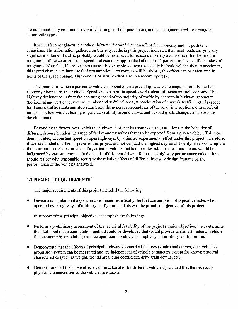
are mathematically continuous over a wide range of both parameters, and can be generalized for a range of automobile types.

Road surface roughness is another highway “feature” that can affect fuel economy and air pollutant emissions. The information gathered on this subject during this project indicated that most roads carrying any significant volume of traffic probably would be resurfaced for reasons of safety and user comfort before the roughness influence on constant-speed fuel economy approached about 4 to 5 percent on the specific patches of roughness. Note that, if a rough spot causes drivers to slow down (especially by braking) and then to accelerate, this speed change can increase fuel consumption; however, as will be shown, this effect can be calculated in terms of the speed change. This conclusion was reached also in a recent report (2).

The manner in which a particular vehicle is operated on a given highway can change materially the fuel econotiy attained by that vehicle. Speed, and changes in speed, exert a clear influence on fuel economy. The highway designer can affect the operating speed of the majority of traffic by changes in highway geometry (horizontal and vertical curvature, number and width of lanes, superelevation of curves), traffic controls (speed limit signs, traffic lights and stop signs), and the general surroundings of the road (intersections, entrance/exit ramps, shoulder width, clearing to provide visibility around curves and beyond grade changes, and roadside development).

Beyond these factors over which the highway designer has some control, variations in the behavior of different drivers broaden the range of fuel economy values that can be expected from a given vehicle. This was demonstrated, at constant speed on open highways, by a limited experimental effort under this project. Therefore, it was concluded that the purposes of this project did not demand the highest degree of fidelity in reproducing the fuel consumption characteristics of a particular vehicle that had been tested; those test parameters would be influenced by various amounts in the hands of different drivers. Rather, the highway performance calculations should reflect with reasonable accuracy the relative effects of different highway design features on the performance of the vehicles analyzed.

1.3 PROJECT REQUIREMENTS

The major requirements of this project included the following:

0

l

0

l

Devise a computational algorithm to estimate realistically the fuel consumption of typical vehicles when operated over highways of arbitrary configuration. This was the principal objective of this project.

In support of the principal objective, accomplish the following:

Perform a preliminary assessment of the technical feasibility of the project’s major objective; i. e., determine the likelihood that a computation method could be developed that would provide useful estimates of vehicle fuel economy by simulating realistic operation of vehicles on highways of arbitrary configuration.

Demonstrate that the effects of principal highway geometrical features (grades and curves) on a vehicle’s propulsion system can be measured and are independent of vehicle parameters except for known physical characteristics (such as weight, frontal area, drag coefficient, drive train details, etc.).

Demonstrate that the above effects can be calculated for different vehicles, provided that the necessary physical characteristics of the vehicles are known.

2

0

0

Demonstrate that a large-roll chassis dynamometer (“dyne”) can apply loads to a vehicle under test to appropriately simulate desired highway features; and, show the extent to which such simulation is required to meet the objectives of this project.

Develop methods for measuring the requisite operational parameters of vehicles to permit preparation of a vehicle data base.

Procure and/or develop instrumentation necessary to support the measurement of needed vehicle parameters.

Test a small number of modern (1980s-era) vehicles and assemble a prototype data base that describes the fuel consumption and exhaust emissions of these vehicles as functions of driveshaft torque’ and such other parameters as would be found necessary. (Exhaust emissions were deleted from data requirements for some of the later tests.)

During vehicle testing, obtain measured operating data for modern vehicles to update existing references giving similar data on older vehicles. Parameters would include; e.g., fuel economy vs. constant speeds, on grades, on curves, while idling, and during accelerations and decelerations-or, under load conditions simulating these. Such data would be obtained to the extent compatible with other project objectives.

* Driveshaft torque or torque is related to force or load on vehicle from road loads, accelerations, grades and curves and has units of Newton meters. For further discussion see Appendix A - A. 1.1.7 and Appendix C- C.2.1.

A fundamental requirement for’this project was to measure the propulsive demands imposed on a vehicle while that vehicle was in operation on open roads and/or other outdoor test facilities. This necessitated measurement of vehicle loads from within the vehicle rather than by an external means, and recording of those data by a system on board the vehicle. It was intended that the instrumentation system would be transferred from vehicle to vehicle; thus, it was necessary to choose a measurement location that afforded external access to the measured part.

Perhaps the optimum test locus to sense only propulsive loads on the vehicle was in the drive train between transmission and drive wheels. This would measure both torque and rotational speed at the same location; torque would indicate tractive force, rotational speed would measure drive wheel and road speeds, while the product of torque and rotational speed at the same point would yield propulsive power. Such a test locus would exclude sensing of engine accessory loads and of losses in the transmission. For rear-wheel-drive (RWD) vehicles, only a single measurement system on the drive or propeller shaft would be required. For front-wheel-drive (FWD) vehicles tested with two separate half-shafts driving the two front wheels, instrumentation had to provide dual measurements of both torques and shaft speeds for each half-shaft individually.

A pilot study was conducted to demonstrate the measurability of the effects of grade and horizontal curvature, and the suitability of the large-roll chassis dynamometer (dyno) to simulate such loads. To determine measurability, an existing instrumented test automobile (1975 Dodge Dart, an RWD vehicle) was further equipped with instrumentation and a digital data logger. The auto was operated on private roads with grades to 8 percent and curves with radii from 240 ft to 2000 ft (73 m to 714 m), at speeds up to 60 mi/h (97 km/h). The dyno was used to measure fuel consumption and exhaust emissions over the full normal operating range of the vehicle; the resultant data yielded a prototype data base for this car that demonstrated the simple format required to describe the observed performance.

To develop data on current (1980- 1981) production automobiles, new, high-performance digital data acquisition systems and two 1980 model-year autos were procured. After exploratory tests at airports relatively near to VNTSC, the Bangor (ME) International Airport was chosen as the primary test site because of its adequate facilities and the willingness of its management to accommodate the necessary tests. Driveshaft torque was measured at a number of constant speeds on the runway and, at low speeds, on the heavy-duty apron of the airport. Torque on curves was determined by running multiple continuous laps of circles with three different radii, at five speeds on each circle to produce lateral accelerations ranging uniformly up to about 0.5 G. The possible difference in curve effect upon an FWD auto (as compared with the RWD cars) was explored after procurement of a third vehicle, a 1981 model with this type of drive train. During some of these tests, the vehicles were equipped with fuel flowmeters to monitor fuel consumption. On one car, two complete sets of tires, both bias-ply and radial-ply, were tested; the other two cars used only radial-ply tires. Some of the test cars were operated on certain public highways in the Bangor area to evaluate potential highway and traffic effects.

Each of the three vehicles was tested, also, on the dyno over the full operational range of speeds and both positive and negative torques, while fuel consumption was measured either by exhaust-gas analysis (for one car) or fuel flowmeter. The exhaust-gas test procedure also yielded exhaust emissions data over the operational range for that car.

In addition to the principal tests described above, limited experiments were conducted to explore related aspects of vehicle operation on highways and to support the planned development of a performance prediction algorithm. A study of 10 different drivers operating one of the instrumented vehicles on a highway with a constant posted speed limit, but otherwise free to drive as they normally would, assessed the influence of driver

5

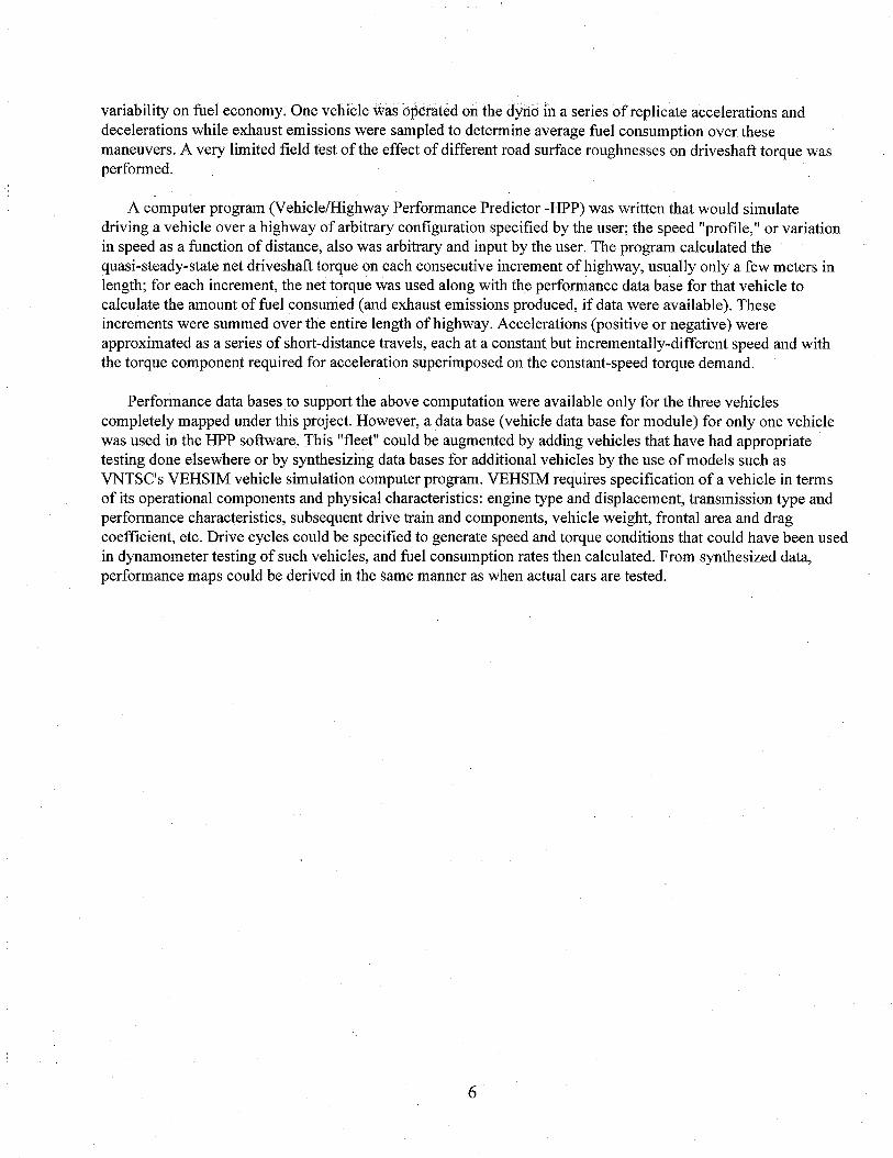
variability on fuel economy. One vehicle Was operated on the dyne in a series of replicate accelerations and decelerations while exhaust emissions were sampled to determine average fuel consumption over these maneuvers. A very limited field test of the effect of different road surface roughnesses on driveshaft torque was performed.

A computer program (Vehicle/Highway Performance Predictor -HPP) was written that would simulate driving a vehicle over a highway of arbitrary configuration specified by the user; the speed “profile,” or variation in speed as a function of distance, also was arbitrary and input by the user. The program calculated the quasi-steady-state net driveshaft torque on each consecutive increment of highway, usually only a few meters in length; for each increment, the net torque was used along with the performance data base for that vehicle to calculate the amount of fuel consumed (and exhaust emissions produced, if data were available). These increments were summed over the entire length of highway. Accelerations (positive or negative) were approximated as a series of short-distance travels, each at a constant but incrementally-different speed and with the torque component required for acceleration superimposed on the constant-speed torque demand.

Performance data bases to support the above computation were available only for the three vehicles completely mapped under this project. However, a data base (vehicle data base for module) for only one vehicle was used in the HPP software. This “fleet” could be augmented by adding vehicles that have had appropriate testing done elsewhere or by synthesizing data bases for additional vehicles by the use of models such as VNTSC’s VEHSIM vehicle simulation computer program. VEHSIM requires specification of a vehicle in terms of its operational components and physical characteristics: engine type and displacement, transmission type and performance characteristics, subsequent drive train and components, vehicle weight, frontal area and drag coefficient, etc. Drive cycles could be specified to generate speed and torque conditions that could have been used in dynamometer testing of such vehicles, and fuel consumption rates then calculated. From synthesized data, performance maps could be derived in the same manner as when actual cars are tested.

6