HILBERT SPACES AN.. (U) NORTH CAROLINA UNIY AT CHAPELHILL CENTER FOR STOCHASTIC PROC.. H KOREZLIOGLU ET AL.

UNLSII~ MAR 86 TR-95 AFOSR-TR-06-0326 F/G 12/1

E hDR 6 5 1 S H A S I C I T E R T I N F O hO E A T R h h h mlRO E S E N /

mnsoonhhh

.6

lin L;,*~132 1.

DIII 12.0

1111 111IIII25'

MICRnr(W' CHAR~T

bv'

AFOSR rR.- 8 6 -0 3 2 6

CENTER FOR STOCHASTIC PROCESSES

Department of Statisticso University of North CarolinaLfl Chapel Hill, North Carolina

00

'U-X

STOCHASTIC INTEGRATION FOR OPERATOR VALUED ~

PROCESSES ON HILBERT SPACES AND ON NUCLEAR SPACES_~

by

H. Korezlioglu

and

C. MartiasCZ)

Technical Report No. 85

March 1986 revision

88 ~ 6034

UNCMfSSIFIED

SECURITY CLASSIFICATION Of THI1S PAGE

* REPORT DOCUMENTATION PAGE

I& REPORT SECURITY CLASSIFICATION lb. RESTRICTIVE MARKINGS

UNCLASSIFIED ________________________2a SECURITY CLAS3IFICATION AUTHORITY 3. DISTRIBUTIONIAVAILABILJITY OF REPORT

NAApproved for Public Release; DistributionNA Unlimited

ft. OECLASSIFICATIlONjOOWN4GRAOING SCHEOULA

4. PERFORMING ORGANIZATION REPORT NUMBER(S) S. MONI1TOR4ING ORGANIZATION REPORT NUMBERIS)

Technical Report No. 85AF RTR 86 2E* &a NAME OF PERFORMING ORGANIZATION Ik6 OFFICE SYMBOL 7&. NAME OF MONITORING ORGANIZATION

* University of North Carolina Ifadani AFOSR/NM

Ua AOORIESS (City. Samare nd ZIP Code) Mb AOORESS (City. Stt a"d ZIP Code)

Center for Stochastic Processes, Statistics Bldg. 410Department, Phillips Hall 039-A, Bolling AFB, DC 20332-6448

* Chapel Hill, NC 27514Q&Ba NAME OF PUNOING/31PONSORING iW. OFFICE SYMBOL 9. PROCUREMENT INSTRUMIENT IOENTIPICATION NUMBER;

ORGANIZATION I(if .eUehbbAFOSR J_______ F49620 85 C 0144

I&. AOORESS lEdty. State ,nd ZIP Code) Ia. SOURCE OF PUNOING No$.

Bl~40PROGRAM PROJECT r TASK WORK UNITElg 1 LE MENT NO. NO. NO4. NO.

* Bolling AFB, DC6.12234 f511I. TITLE (Ineloade Security Cealikasiono

Stochastic Integration for Operator Valued Proi esses on Hil ert Sn~acej and on Nucl.ar SpaCs12. PERSONAL AUTHORI(S)

H. Korezlioglu and C. Martias*13a. TYPE OP REPORT 13b. TIME COvEREG11 14. OATS1 OP REPORT (Yr.. .11.. Day) is. PAGE COUNT

*technical FROM. TO2,L.2. March 1986 revision -q* 1B. SUPPLEMENTARY NOTATION

*17. COSATI COOGS IF I SUBJECT TERMS VCongdinu on ,pffb if ncessw7 a" idIIdfy by block 0nn0"atD

FIELO GROUP $sU. GPI. IKeyords: Stochastic integration, Hilbert space valuedsxxxx xxquare integrable martingales, representation of square Iintegrable martingales.

IS. ABSTRACT (Conaln..* on nmv.? it tweWSM07 @Ad IdOXtifY 6y Weeck uMnbrl

The representation of a nuclear space vlaued square integrable martingale by means ofF another nuclear space valued square integrable martingale is given in terms of stochastic

integrals of operator valued processes. The construction of the stochastic integral

goes through that of operator valued processes on Hilbert spaces. A new approach is

* given for the Hilbertian case, so that only the integration of Hilhert-Schridt operator

* 'alued processes is needed to represent square integrable martinloales.

L20. OISTRIBUTION/AVAILABILiTY OF ABSTRACT 21. ABSTRACT SECURITY CL.ASSIFICATION

UNCLASIFfIEOUNLIMITED X3 SAME AS NP?. 2OTIC USERS UNCLASSIFIEDI22a. N1AME OF RESPONSIBLE INOIVIOUAL 221X TIELEPM.ONE NUMBS9L)C' 2c OFFICE SYMBOL

'incii.t * , Coda'

-'~~ AFOSR/NM- ~~~e-* -' .. 1 ~... .. ~~-.-.-.-... ~ * ~:~~ . * I NCIA' TFI.EQ

*iV .. .. - . -,?fi2 -. . ,i , ii . . r , A A A.- - - - -. .- :.i - i .. ,- :.w- *7: . . :.: =. . '. -

STOCHASTIC INTEGRATION FOR OPERATOR VALUED

PROCESSES ON HILBERT SPACES AND ON NUCLEAR SPACES

Accession For

by NTIS RP &I

DTIC TA'• ~ ~~~Unannrn- c. d[-

H. Korezlioglut Juztific:.B y -- t

Center for Stochastic ProcessesDepartment of Statistics --- ----

University of North Carolina Avail- -

Chapel Hill, NC AvDist -

and

C. Martias -

Centre National d'Etudes des T6lcomunicationsIssy-les-Moulineaux, France 'NSPErED

Abstract The representation of a nuclear space valued square integrable

martingale by means of another nuclear space valued square integrable martin-

gale is given in terms of stochastic integrals of operator valued processes.

The construction of the stochastic integral goes through that of operator valued

processes on Hilbert spaces. A new approach is given for the Hilbertian case,

so that only the integration of Hilbert-Schmidt operator valued processes is

needed to represent square integrable martingales.

Keywords : Stochastic integration, Hilbert space valued square integrable

martingales, nuclear space valued square integrable martingales, representation

of square integrable martingales.

Research supported by AFOSR Contract No. F49620 82 C 0009. C O'

F'j1G~~ q6,

. .X % .. ? . ..:.:.. ... .... . . .... . . . . . . .". . -.. . -. ..".... . ,--. . ..-.-..-.. ."-

.". .- . . ..--. .-... . . ... ... '..'-..< ...->',.,

1

INTRODUCTION

This paper deals with the integration of operator-valued stochastic pro-

cesses with respect to Hilbert space and nuclear space valued square integrable

martingales.

Generally speaking the stochastic integration for operator valued processes

can be described as follows. Let (Q,A,P) be a complete probability space with a

filtration (Ft; t'R++) ; (F,F') and (E,E') be two pairs of topological vector

spaces in duality, and let M be an F'-valued square integrable martingale. We

suppose, in this introduction, that the notion of F' (and E')-valued square

integrable martingale and the space L E(,A,P) of square integrable random va

riables with a locally convex topology are well defined. An elementary process

with values in the space of continuous linear operators from F' into E' is

defined as follows.

n{o}xBoLo + i=o Jti'ti+1 1]xB Li

where to = 0 t<t2< < tn+1 I Bi E Ft and L is a continuous linear operator

from F' into E'. Then the integral of X with respect to M can be defined as the

usual Stieltjes integral

nf XtdMt 1 LB0LoMo + I I B Li(Mt+ " t

This quantity defines an E'-valued random variable. The main problem of the

stochastic integration with respect to the given F'-valued square integrable

2martingale M is the definition of a topological vector space, say S2, of random

functions with values in the space of linear operators from a certain space

into E', generated by the vector space V of elementary processes as given above

so that the mapping X -f X dM defines an algebraic and topological isomorphism

+m

t '

r.:-'.'._'..3-,/ ; ;. > . 3; " " :< "-" -:- '',, ." "",;, '' / ",'"_"", - " "::Y -'".' "' ''

i%.p

2

2 2of V into LEA (,A,P). The stochastic integral of an arbitrary element of S2 I.-

would then be defined by the extension of this isomorphism to S2. Partial

stochastic integrals would also give F'-valued square integrable martingales.

The stochastic integral for operator valued processes on Hilbert spaces

with respect to a Brownian motion was considered by Curtain and Falb [3],

Daletskii [41, Gaveau [81, Kuo [15], Lepingle and Ouvrard [16], Yor [311, etc ;

(cf also [5], [6] and [19] for definitions, applications and references) ;

and the stochastic integral with respect to an arbitrary Hilbert space valued

square integrable martingale by Kunita [141. But the first extensive definition

of the stochastic integral in the last case is due to MKtivier and Pistone [20)

who showed that processes in S2 may take values in a space of noncontinuous

operators. Important applications of Mtivier and Pistone's approach were made

by Pardoux for the study of stochastic partial differential equations [241, by

Ouvrard for the representation of martingales [22] and for the linear filtering

of Hilbert space valued systems [23], and by Martias for the derivation of the

nonlinear filtering equation for Hilbert space valued semimartingales [17], [18].

In a work [12] dealing with the derivation of the nonlinear filtering equa-

tion related to a Hilbert space valued nonlinear system driven by Brownian

motions, the first author showed the equivalence between stochastic integrals

with respect to a Hilbert space valued Brownian motion in the sense of M~tivier

and Pistone and stochastic integrals with respect to the corresponding cylindri-

cal Brownian motion. He also obtained the nonlinear filtering equation in terms

of the corresponding cylindrical innovation process where the covariance operator

and its pseudo-inverse do not appear explicitely as in [173, [181 and [231. In

[131 we extended the same method to the case of distribution valued nonlinear

....................... . .......-.. • ° .

3

systems driven by distribution valued Brownian motions. For this case, a cons-

truction of the stochastic integral can also be found in ltO's work [9]. In

[12] the passage from a Brownian motion M to a cylindrical Brownian motion

reposes on the fact that, in this case, Q is constant and dtMI - adt with a

constant a. The introduction of adequate predictable fields of Hilbert spaces

enables the extension of the same method to the case of arbitrary square inte-

grable martingales.

In Section 1 we consider the stochastic integration with respect to a

Hilbert space valued square integrable martingale and propose a method of cons-

tructing stochastic integrals and show that the set of martingales-obtained by

Ithis method is the same as that obtained by M~tivier and Pistone's method. Our

method leads to some interesting algebraic and topological isomorphisms useful

for the construction of stochastic integrals and representations of square

integrable martingales.

In Section 2 we deal with the extension of the method to nuclear space

valued square integrable martingales as defined by Ustunel in [29]. The extension

i based on the fact that in the setting of [9], every nuclear space valued

square integrable martingale M has almost all of its trajectories in a Hilbert

space H. But in general H is not unique. Although the increasing process <M>

corresponding to a martingale M can be defined independently of H, the represen-

tation d<M>= Q dIMi depends on H. The entire approach uses a particular

representation, but the set of all square integrable martingales obtained by the

method developed here does not depend on the chosen Hilbert space H.

We end the paper with a short section of examples and applications where we

consider the white noise process as a distribution valued one corresponding to

* the classical definition of the white noise as the derivative of the Brownian

," .... .'.'. "." ..',.'.:'...'.€ . ...'................... ............... ... ............... ....... ....... *......'.. .-.-

~ *% ~% * .~P .* .*.~%.**'~**~*or,*... *..,isp.J....t..-..% > % **~% .*.~ .v~/. :..K.%%.~:%c.:.!. (

4

motion in the sense of distributions. We show that the stochastic integral

with respect to the white noise process is equivalent to the classical Ito

integral.

1. STOCHASTIC INTEGRATION WITH RESPECT TO HILBERT SPACE VALUED MARTINGALES.

1.1 PRELIMINARIES

All the Hilbert spaces considered here are real. H and K represent

separable Hilbert spaces. Scalar products and norms are denoted by (,,.)

and 1I1I, respectively. In order to point out, if necessary, the-space on

which they are defined, they will be indexed by the symbol representing the

space.

L(H,K) is the space of bounded linear operators from H into K with uniform

Inorm f*Ij, also denoted by '1.''HK for more precision. LI(H,K) is the space of

nuclear operators with the trace norm 11'11, or tr(.), also denoted (''HlKif necessary and L (HA is the space of Hilbert-Schmidt operators with the

Hilbert-Schmidt norm I' 2 ,written also as 1 I'{IH2K" 1 •l K(ep 2 K

conveniences, H *l K (resp. H 2 K) are identified with LI(H,K) (resp. L (H,K))

under the isometry which puts h a k into one-to-one correspondence with (.,h)Hk

for h ( H, kc K.

Unless the contrary is mentioned, we identify Hilbert spaces with their

topological duals. We shall construct many pre-Hilbert spaces becoming Hilbert

spaces after being divided by an equivalence relation. In order to simplify

the presentation and the notations we shall identify this kind of pre-Hilbert

spaces with the corresponding quotient Hilbert spaces.

..................... .... ...... -... ....-...-.........-.".."',-..'

The transpose of a linear operator A is denoted by A*, its domain by

Dom A and range by Rg A. The closure of a set S is denoted by S.

The algebraic and topological isomorphism between two topological vector

spaces E and F is indicated as E 2 F.

For the terminology of stochastic analysis used here we refer to [7] and

[191.

All random variables and processes are supposed to be defined on a comple-

te probability space (0,AP) with a filtration F = (Ft ; tP +) satisfying the

usual completeness and right continuity conditions. We take A = F Adapted

processes, predictable processes, martingales, etc. are with respect to F.

P will represent the a-algebra of predictable sets of B a F. where B+ is the

Borel a-algebra of R. A' stands for R x A.

The equality between separable Hilbert space valued martingales is an

equality up to an evanescent set in S'. Such martingales are defined as those

having cadlag (right continuous and left limited) trajectories, (except on an

evanescent set). For two square-integrable martingales M and N, with values in

H and K, respectively, there is a unique H K-valued cadlag process with inte-

grable variation, denoted by <M,N> and called the oblique bracket of (M,N),

such that M s N - <M,N> is a H 61 K-valued martingale, vanishing at t=o. The

bracket <M,M> that we denote by <M> is called the increasing process of M. We

put JMft:-lI<M>tJl. This process is the unique real predictable increasing

process with integrable variation for which IIMI - MI is a martingale vanishing

at t=o. We shall denote by M (H) (resp. M(H)) the space of all H-valued square

integrable (resp. continuous) martingales.

From now on M will represent a given martingale in M2(H) and X will denote

the measure defined on P by dPdMt. There exists a predictable process Q with

values in the cone of symmetric and nonnegative elements of LI(H,H), unique up

• .-.-, -o .-., -: "-" .-:-"". .7..-.. . .-.. ""..'-.-.•-...... ..- " .-.' '.-.':'°J"".:-'. L-"",.-'1i

6

to a A-equivalence, such that IIQ11 1 A-a.e. and <M>t= ftQsdlMfs.

In what follows in this first paragraph, D represents a L 2(H,H)-valued

*2

the positive square root of Q. Let L 2(D,HK) be the space of processes X defi-

ned as follows for A-almost all (tw)e 0l' ,Xt(w) is a (not necessarily conti-

nuous) linear operator from H into K such that Rg D t(w)c Dom X t(w). (Xt o D

to R+) is a predictable process with values in L 2(H,K) and f sIItycw) .Dt(w)H 1*22

A(dt,dw) <-n. The space L *2(D,H,K) is complete under the Hilbertian seminormi

X...[fr I I X(w) oD t(w)II 12A(dt,di)]11 , (cf. [19]). A2(D,HK) will denote the

Hilbert subspace of L.~ generated by all L(H,K)-valued processes X in L' such

that (Xth,k) is a real predictable process for all h in h and k in K. The set

of all L(H,K)-valued elementary processes of type

n

(1.1.1) X 1 (O} xB A0 + 1 1 i A1i

where o t tt< t2. A e L(H,K) and B1 ~ is deseF A2(D,H,K).0 1 2.. t

The space A 2(D,H,K) was introduced, with D = 12 by Mttivier and Pistone

in [20] for the definition of the stochastic integral with respect to M. We shall

denote A2 (D,H,F{) by A2(D,H).

The stochastic integral of an elementary process of type (1.1.1) is the

ordinary Stieltjes integral

n(1.1.2) !IR Xt dMt 1 'B A 0(M0) + I 1B. AMt -Mt)

+ 0 10o 1 i+1 1

As lx! 2 E I1fjRX dMtI , the integral extends to A (D,H,K) by isometry.

Freach Xe A 2 (.-,..,K. ft UM defines an element of M2(K), denoted by X.M. 710- .

7

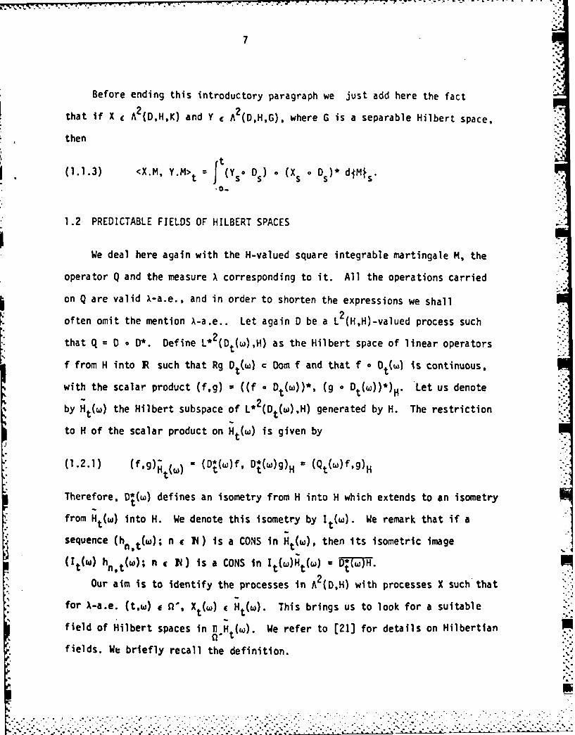
Before ending this introductory paragraph we just add here the fact

2 2that if X C (D,H,K) and Y e A (D,H,G), where G is a separable Hilbert space,then

(1.1.3) <X.M, Y.M>t = (Yso Ds) o (Xs o Ds)* djMts.

1.2 PREDICTABLE FIELDS OF HILBERT SPACES

We deal here again with the H-valued square integrable martingale M, the

operator Q and the measure X corresponding to it. All the operations carried

on Q are valid X-a.e., and in order to shorten the expressions we shall

often omit the mention X-a.e.. Let again D be a L2 (HH-valued process such

*that q = 0 - D*. Define L*2 (Dt(w),H) as the Hilbert space of linear operators

f from H into IR such that Rg t (w) c Domn f and that f oa t is continuous,

with the scalar product (f,g) -((f - Dt()* (g o Dt(w))*)H. Let us denote

by Ht(w~) the Hilbert subspace of L* (Dt (w),H) generated by H. The restriction

to H of the scalar product on Ht (w) is given by

*(1.2.1) (f,g)-( (D*(w)f, D*(w~g)H (Q (co)f~g)H

Therefore, D*(w) defines an isometry from H into H which extends to an isometry

*from H (w) into H. We denote this isometry by It(w~). We remark that if a

*sequence ( t(w;n c IN) is a CONS in Ht (w), then Its isometric image

(I (w) h tMw; n c IN) is a CONS in It MHt) M D*(w)H.2

Our aim is to identify the processes in A (D,H) with processes X such that

for A-a.e. (t,w) e 0', X (w) c Ht(w). This brings us to look for a suitable

field of Hilbert spaces in n H w.We refer to [21) for details on Hilbertian

*fields. We briefly recall the definition.

31" -. _. . X77 VRT -77. -77

DEFINITION 1.2.1. A predictable field of Hilbert spaces in Ht(w ) is a vector

subspace E having the following properties.

(i) For all f and g in E, the mapping (t,w),.(ft(w) g ))t defnes a V"

predictable real process.

(ii) Any h £ T. Ht(w) such that (ht(w), ft(M))-tl) is predictable for

all f e E belongs to E.

(iii) There exists a sequence f = (fn; nell) in E such that the sequence

f(fn(w)- n V) generates Ht(w).

We choose an arbitrary linearly independent sequence e = (en; n-ll) gene-

rating H and consider the sequence etlw) = (en,t(w); nctN) defined x-a.e.

recursively as follows.

n-1 "e ot(w): = e and en,t(w):= en - k o(en,ek't(w)) t (w) ek,t(w) for n1,

with': (1. 2.2) :ent(w) = enlt()Ien,t(w)IIjt(,) if Ilen,t(w)IIt(W) >o

- o if leen,t(w)II tkw) = 0.

The nonvanishing terms of et(w) form a CONS in Ht(w).

The sequence e will play the same role as f in the'property (iii) of the

above definition. Before giving the characterization of the predictable field

we shall be using here, we consider some predictable processes playing an impor-

tant role in what follows.

Q is a predictable process, i.e. for all f,gc H, (Qt(w)fg)H =

is predictable. Therefore, by construction, all the e.'s are predictable. More-

over Q has the following representation (as a process with values in

L2(H,H) LI(HH)).

"w.'',-''-. ' '.-''-.'':' -,' -.''- '."' -- :."."< ,"' "- ."-*' " " " "-, -. -- . '-"-. -. "'-"'" ." .""- "- "" .""" ' ". "'.-' '. '. ': ' 7 .- ,'

9

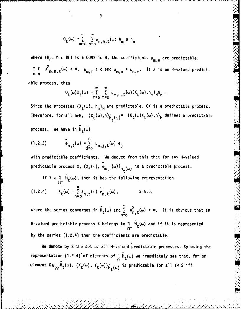
Qt(w) I im ~(w) h auh nm=o n ~f~to

*where (h; n c IN) is a CONS in H, the coefficients Vmn are predictable,

Et E 1 m,n,t(w) < V'1m'm >, o and P m,n = in,m* If X is an H-valued predict-

able process, then

M~~m n~

* Since the processes (X (w), hm) are predictable, QX is a predictable process.

* Therefore, for all hcH, (Xt (w),h)H w (Qt(w)Xt(w),h)H defines a predictablet

* process. We have in Ht(w)

- n*(1.2.3) en() M ui Mw e.

n~ jon,j,t .1

* with predictable coefficients. We deduce from this that for any H-valued

* predictable process X, (Xt M. emt(w))-( is a predictable process.

If X c HtH M, then it has the following representation.

(1.2.4) Xt) M a Mw e M), A-a.e.t n,t n,t

where the series converges in Ht M and I a2 (w) < It is obvious that antn-o t

H-valued predictable process X belongs to HI Ht(w) and if it is represented

by the series (1.2.4) then the coefficients are predictable.

We denote by S the set of all H-valued predictable processes. By using the

* representation (1.2.4) of elements of ii Ht (w) we imediately see that, for an

element Xe nHtMw) (Xt(W). Yt(W))-( is predictable for all Ye S 1ff

H t~pJ

10

measurabity of( ~) n~)- for all Y e S does not depend on the chosen

*particular sequence e.

Moreover, if (X t(u)),h).. is predictable for all heH, then (1.2.3) impliesH t(W)

that (X (w), (w) is predictable for all n. Conversely, if this is the case,

(xt(w),h). is predictable for all h c H, because any constant process with

H t(W)

values in H is a particular H-valued predictable process.

We denote by E(D,H) the vector subspace of n H t(w) consisting of all

elements X such that (Xt~) M. (w))- is predictable for all n 6 IN. ThisHt~

is the set of all elements X such that (X t(w). Yt (w))- is predictable forH t(w)

all Y e S. Therefore, E(D,H) does not depend on 6. E(D,H) is a predictable

field of Hilbert spaces and said to be generated by S. We remark that E(D,H)

is the set of all elements X such that (Xt(w),h)- is predictable for all h g H.Htt

The elements of E(D,H) are called predictable fields of vectors.

A2(D,H) will be the Hilbert space of all elements X of E(D,H) such that

(1.2.5) IIX112 = i J It(w)JI )A(dt,dw) <A2 Hl H(W)

*A'(DH) is the space of all elements X of E(D.H) whose representation in terms

*of e as in (1.2.4) is such that

(1.2.6) IIX11 2 a 2 a' X (dt,dw) <-2 n o n t~wA l

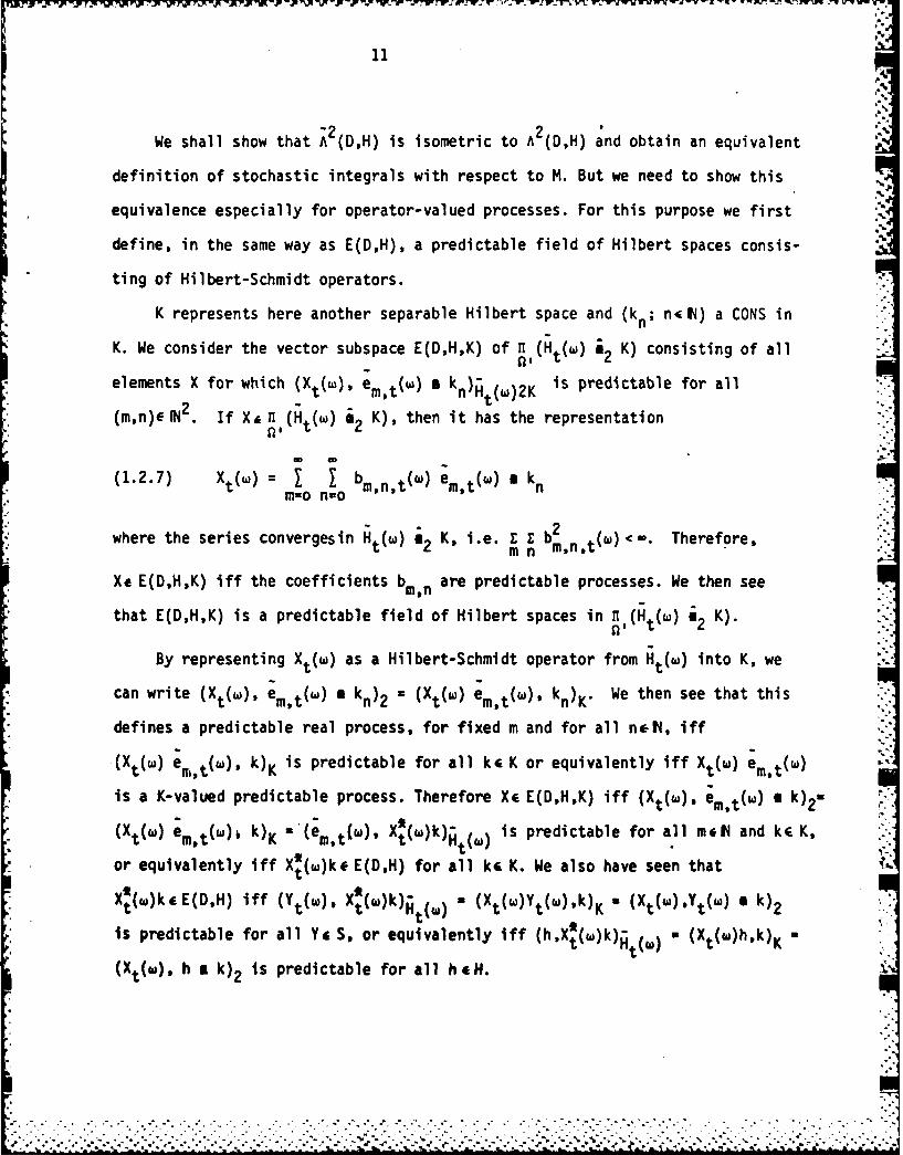
2 2We shall show that A (D,H) is isometric to A (D,H) and obtain an equivalent

definition of stochastic integrals with respect to M. But we need to show this

equivalence especially for operator-valued processes. For this purpose we first

define, in the same way as E(D,H), a predictable field of Hilbert spaces consis-

ting of Hilbert-Schmidt operators.

K represents here another separable Hilbert space and (kn n<IN) a CONS in

K. We consider the vector subspace E(D,H,K) of n (Ht~)' K) consisting of all

elements X for which (Xt(w), emt(w) a kn~~w~ is predictable for all

2(m,n)eIN .If X& n (Ht~)' K), then it has the representation

(1.2.7) Xt(w) = 1 t~w emt(w) aknni=o n=o

where the stw ,ie eries convergesin K, i me b ~~tw Therefore,

Xt E(D,HK) 1ff the coefficients bmn are predictable processes. We then see

* that E(D,H,K) is a predictable field of Hilbert spaces in ni (Ht~)~ K).By~ ~ ~ ~~~~w rersnin t2 ro noK

Byrereetig t~)as a Hilbert-Schmidt operator fro Htw)int K we

can write (Xt(w), em,t(w) *kn) 2 =(Xt(w) eni,t(w), k n)K* We then see that this

*defines a predictable real process, for fixed m and for all nt.?N, 1ff

(Xt(W) ,t (w), k)K is predictable for all kr.K or equivalently 1ff Xt(w) mtw

is a K-valued predictable process. Therefore X* E(D,H,K) 1ff (Xt(w), em,t(w) a k)2-(xt(W) e ,(w)j k) ='(em,t(w), Xt(w)k)( is predictable for all m*IN and kfEK,

or equivalently 1ff X*(w)kt E(D,H) for all kr& K. We also have seen that I.

X 2(w)kfE(D,H) 1ff (Yt(W), X *(w)k)( (Xt(w)Yt(w),k)* (Xt(w),Yt(w) a

is predictable for all Y& S, or equivalently 1ff (h, * w~ (Xt(w)h,k)

(Xt(w). h a k)2 is predictable for all h el.

12

Therefore, we see that the definition of E(D,H,K) does not depend on the

chosen sequences (en; ncIN)cH and (k n; neIN)cK and that E(D,H,K) is gene-

rated by (Yt(w) k; Ya S, k K) as well as by constant processes with values

in H a K, (the tensor product is taken on Ht(w) '2 K).

Now we define A2 (D,H,K) as the Hilbert space of all elements X in E(D,H,K)

such that

-22

-.. (1.2.8) IlXll 2: = f l~( lIt )K

we see that A2(D,H,K) consists of those elements X having the representation

(1.2.7) with predictable coefficients such that

(1.2.9) IIl2 f b2 (w)x(dtdw)Im n a' mn't

The construction of A (D,H,K) suggests the following statement.

PROPOSITION 1.2.2. A2(D,H,K) " A2 (D,H) i2 K.

Proof The set of elements of type

M N(1.2.10) it(w) = I bmn,t(w) em,t(w) * kn a t()) '2 K

i~n=oM N 2 -2

where (kn; nc N) is a CONS in K and I I f bm 4<,is dense in A(DHK).m=o n=oA n

N Define X6 A2(DH) i2 K byn Yn @ kn where Yn is the H-valued predictable pro-

cess defined by Yn,t(w) = 1o bm,n,t(w) em,t(w). We see that IJXiI I IX'll.

The mapping X-,.X' extends to an isometry I1 of A2(D,H,K) into A2(D,H) s2 K.

Conversely, if YEA2(D,H) is represented by Yt(w) a m,t(w) em,t(w) and if

-2 a -- -2 2 twa * keA (D,H) K, we define XA (D,H.K) by Rt()=m t(W)(mt(w) a k).

Ma.

............ . . .

..' . . " ''*" ' -.- ',.."' .".. .""'"'. ..w.' '- :d '- " ,"" .' . .' -"" . '.,..,'.-. . " '--D ," " " -" " ' """" """ "

13

We see that 11I - xIIll. The mapping X'- X then extends to an isometry 12

from A2(D,H) a2 K into A (DH,K). Since I1 2Y a k = Y a k A2 (DH) s2 K,

I is the inverse of 12 and the two isometries are onto. 0

22 %

According to the above proof if X' A(D,H) '2 K is represented by

Km c m,n X m kn=o no

where the coefficients are real and E c2 c - , (X ; nN)cA (D,H) andm n mn -n

(kn; neIN)c K are orthonormal sequences, then the isometric image X of X'

n A2(D,H,K) can be represented by

Xt(W ) = m,n X m,t(w) a k -a.e.M=o n=o

where the tensor products are taken in Ht(w) @2 K and the series convergesin

-2A (D,H,K).

The following theorem will allow a definition of stochastic integrals,

equivalent to that of M~tivier and Pistone in [20].

-22THEOREM 1.2.3. A2(DH,K) a, A2(DH,K).

Proof : (kn; nat) is again a CONS in K. Let Xe A2 (D,H,K) be given by

(1.2.10) and let us define X by

M N*(1.2.11) Xt~w) m e~(w) a kne H K

nxttw m) -ak n " 2muo n~o

where the tensor product is taken In H a2 K. X is predictable and

.. . .. . . . . . . . . . ... . .

Si.7.. 0. - k ... . . '. -. .*S. . . . '9 *~ * . . . . .

14

M NX t(w) b = ~ ~ tw (D()i (w)) a k

t

Since (Dt(w) emt(w); mefl) is a CONS in It(w)Ht(w), this gives us the represen-

tation of the Hilbert-Schmidt operator Xt(w) Dt(w) in terms of an orthonormal

sequence in H 42 K. We then have

2= 2

MN X 2 fa I-2*w (xd~w

2-

A 2(D,H,K).

Conversely, let XE-A (D,H,K) be L(H,K)-valued. Then X-a.e. Xt(w), tw

is a Hilbert-Schmidt operator from H into K that we can represent by the following

series.

(1.2.12) Xt(w) *Dt(w) = d ()D t(w)e 'tw)) s km,n,tw) tn~'' fM=o n=o

+ c mnt(w) hm a

ni=o n=o

where (h M m&fI) is a CONS in the orthogonal complement of It(w)HtGw) in H and

of course the coefficients are predictable. But we have cn t(w) z o for all

m,n ; because, for all ho H, (hm, D (w)h)H - o, i.e. Dt(w)hm a o, and hence2c mnt(w) = (Xt(w) o Dt(w)hm~k n)K o . Therefore, we have IIXt(w) Dt(W)IIH2K

d2 ( ntw). Now, let us define Xby

(1.2.13) it(w) a dmn(i)e~~)*km o n o

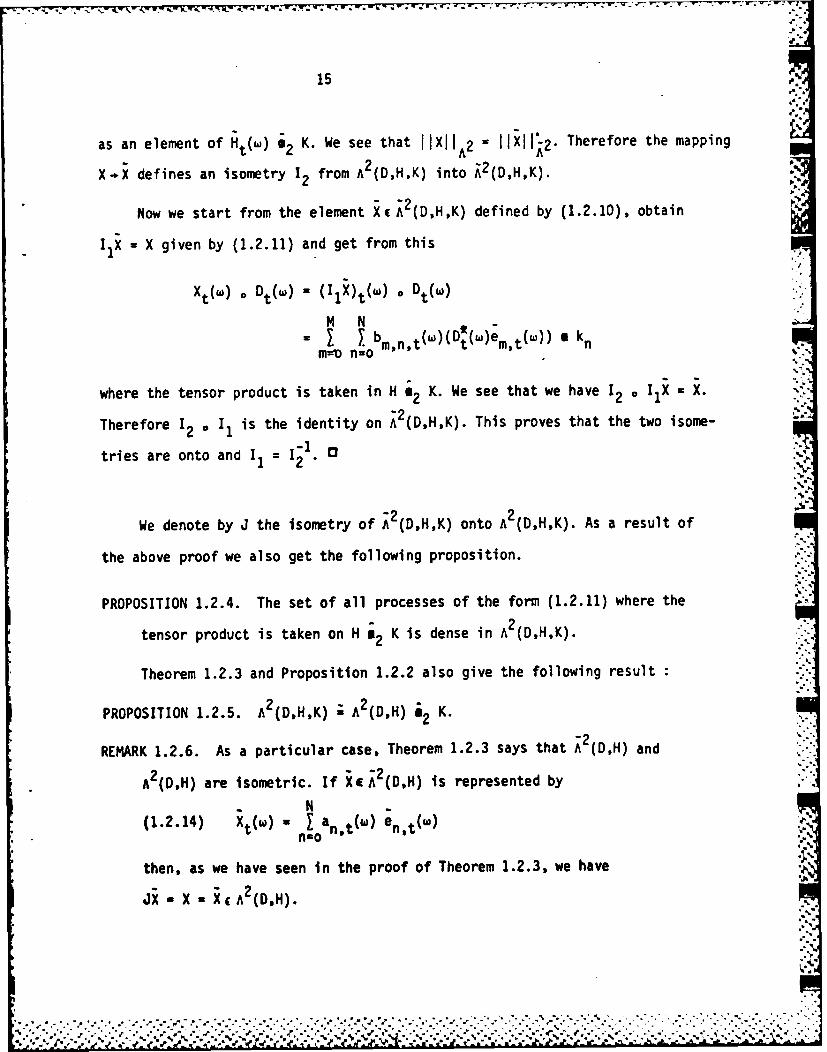
15

as an element of Ht(w) ;2 K. We see thatofHxll2 -IIxIl 2. Therefore the mapping

2X.X defines an isometry 12 from A2(D,H,K) into A2(D,HK). p.

Now we start from the element XA 2(D,HK) defined by (1.2.10), obtain

IX X l given by (1.2.11) and get from this

Xt(w) Dt(w) - (IX)t(w) o Dt(w)

M N- . .bm n,t(w)(D t(w) m,t(w)) kn

m=- n=o

where the tensor product is taken in H a K. We see that we have 2 I^ .-2'

Therefore 12 0 11 is the identity on A2(D,H,K). This proves that the two isome-

tries are onto and I -1 13'

1 2

-2 2

We denote by J the isometry of A2(D,H,K) onto A2(D,HK). As a result of

the above proof we also get the following proposition.

PROPOSITION 1.2.4. The set of all processes of the form (1.2.11) where the

tensor product is taken on H a2 K is dense in A2(D,H,K).

Theorem 1.2.3 and Proposition 1.2.2 also give the following result

PROPOSITION 1.2.5. A2(D,H,K) A A2(D,H) i2 K.

REMARK 1.2.6. As a particular case, Theorem 1.2.3 says that A (D,H) and

A (DH) are isometric. If XeA (D,H) is represented by

(1.2.14) Xt(w) = a (w) e()n,t n,t~w

then, as we have seen in the proof of Theorem 1.2.3, we have

Ji aX XA 2 (D,H).

'a

- . . . . .... . . . .

16

Therefore, J is an isometric injection on the set of all processes of type

(1.2.14). We have even more. If X is an H-valued predictable process such

that ID,( )Xt(w)II )(dt,d ) - then it belongs to both A(D,H) andt~)X(" I H

2A (D,H) and has the same norm in both of them. The set of all processes of-2 2

this type generates the two spaces. We see that A (D,H) and A (D,H) only

differ on the completion of their vector subspace of all H-valued predic- I"table processes. .i

1.3. STOCHASTIC INTEGRALS

We continue to use the notations of Paragraph 1.2. In Paragraph 1.1 we

have seen the definition of the stochastic integral for a process in A2 (D,H).

We adopt the same definition for all H-valued processes in A (D,H). We have seen

that they also are in A (D,H). If X is such a process, then E(fR+XtdMt)2 - lIxIIA2

= 0lXl 2. The stochastic integral of is then well defined and we put

(1.3.1) Mn,t:= o ensdMs (en M)t

We remark that

(1.3.2) <Mm,Mn> ft (e (u), en())s- dfMs (w).<'nt o- M's n,s H5(w s

= {t if n =m, o if n Am.

Hence (Mn; n14J) is a sequence of strongly orthogonal martingales.

-2 2Since the set of processes of type (1.2.14) are dense in A2 (D,H) and A (D,H)

the stochastic integral of an arbitrary element X eA (D,H) is defined as the

limit in L2(fl,AA') of the integrals of an approximating sequence of type (1.2.14).

P''---"" . .' ''. . . . . . . . ...... . ..." "- - - - . . . -. "---.-"'"-... "-

.J..K'1J~- .- '~ p v V K --

17

Consequently, if iE A2 (DH) is represented by (1.2.4) we define

(1.3.3) XtdMt = SNR antdMnt 1,+n o +

with the series converging in L2(a,AP). Obviously, the random variable defined

by (1.3.3) coincides with the stochastic integral of X - JX in the sense of

M~tivier and Pistone.

For an element XeA2 (D,HK) having the representation (1.2.7) with the norm

given by (1.2.9) we define the stochastic integral by

(1.3.4) fS+ XtdMt - (i b m,n,tdM mt)kn+m=o nwo +mntmtn

where the series convergesin L K(a,AP). We have

t112~

(1.3.5) E Rt tll -illi-2

It is obvious that the value of the stochastic integral (1.3.4) does not

depend on the particular representation of X.

The correspondence between this definition of stochastic integrals and that

given by Mltivier and Pistone is not straightforward as in the case of functional

valued processes. The result is given in the following theorem.

THEOREM 1.3.1. Let icA 2 (D,H,K) and let X - JxeA2 (D,H,K). Then the stochastic

integral of X in the senseof (1.3.4) and the stochastic integral of X in

the sense of Mtivier and Pistone coincide.

Proof: If Xis given by (1.2.10). then X JX is given by (1.2.11). It is

obvious that f+XdM in the sense of (1.3.4) and f XdM in the sense of MNtivier

and Pistone coincide. Since the set of processes of type (1.2.10) and the set of

i ~ .5.--. i.................. ................................ ',•-"", ,,, _ S . .•~j* . -,.,- .: -,. . .- ',_, , .- ,.

18

processes of type (1.2.11) are dense in A2(D,H,K) and A2(DH,K), respectively,

we obtain the statement of the theorem.m

rFor a process iei 2 (D,H,K) we denote by X.M the square-integrable martin-

gale defined by t- XsdMs" Theorem 1.3.1 says that X.M = (JX).M, the stochasticae i ai

integrals of the right-hand side being defined in the sense of Mtivier and K-

Pistone. All along this paper the stochastic integrals are defined in the sense

of (1.3.4). If ever a stochastic integral is defined in the sense of M~tivier

and Pistone we will always precise it.

PROPOSITION 1.3.2. Let A2(OH). Then

(1.3.6) <X.M t =t- IlIs(l 2w) d M(-) ( .

Proof Let X (resp. XN) be represented by the right hand side of (1.2.4)

(resp. 1.2.14), then (XN) converges to X in A2 and (XN = JXN = XN; NI)

converges to X = Ji in A2 (D,H). Consequently, there is a subsequence (XN; ieiN)

such that fot IIXNi,s(w)i s(w)dfMIs(w) converges a.s. to ftIIXs(w)II (w)dfMs(w)

and to <X.M>t. (In this last expression X.M is computed by means of M~tivier

and Pistone's integrals). Since X.M - X.M and hence <X.M> = <X.M> with the inte-

gral X.M computed in the sense of Mdtivier and Pistone, (1.3.6) holds.o

Let G be another separable real Hilbert space. Then by approximating the

elements of A2(D,H,K) and 2 (D,H,G) by finite sums of type (1.2.10) we can

similarly prove the following result.

PROPOSITION 1.3.3. Let iEA 2(D,H,K) and ycA 2(D,H,G)

then

(1.3.7) <X.M,Y.M>t d foY 5 Xs •M

•-- -, , '-"-.', . ."-'-'.,: -'.. .-......... -'---'-- -i.;'-'-,"-.T .i . .T- "-'-'-'-.i - - ." . "." "

19

We shall need in Section 2 the following result.

PROPOSITION 1.3.4. Let K and G be separable Hilbert spaces and A a continuous 1

2linear operator from K into G. Then for XEA (D,H,K) we have the following

martingale equality

(1.3.B) A tX dMs f t_ AoX dMs

Proof It is easy to see that (1.3.8) holds for all processes X of type

-2" (1.2.10) in A (D,H,K). Then the equality (1.3.8) is obtained for an arbitrary

process X by the density of processes of type (1.2.10) in A2 (D,H,K). 0

We reproduce here the following representation theorem proved in [221

with stochastic integrals defined in the sense of M6tivier and Pistone. We have

however seen in Theorem 1.3.1 that we obtain the same set of martingales with

the integrals defined by (1.3.4).

THEOREM 1.3.5. Let M and N be square integrable martingales with values in H

and K, respectively. Then there is a process Xe 2 (D,H,K) such that

(1.3.9) N = X.M + NJ

where N is an element of M 2 (K) orthogonal to M. This representation of N

is unique in the sense that X is unique up to )-equivalence and N4 is

unique up to an evanescent set.

According to this Theorem M Itself must have a representation by stochastic

integrals. We express this representation in the following proposition.

PROPOSITION 1.3.6. We have

Mt I fto Is) dMs.t 0 s s

4"~ j'

20

where Itlw) is the isometry of Ht(w ) into H. If (h nc) is a CONS

in H then we have Dt(w) 0 = n n* * hn{ e '2 H.

Proof. Let (h , n IN) be a CONS in H. Then the identity operator onn

H can be fornally represented by i = Lo h h This means that each elementnzo n n'

h • H is represented by h n In(h,h n)Hhn For f,g c H we have (i • Dt(w)fg)H =

(ft 'g n ,g. (Dt(w)hnf)H ([n(Dt(W)hn) f,g)t H ?ngH [E

Therefore, i • t() has the following representationt

i Dt(w) (D()h) . h H ; H. According to the proof of Theorem 1.2.3.t n t n n 2

the isometric image of i is X ( nwo hn h" H(W) H.

For f e Ht(w) we can write

(W)f E n-(h ,f) hn E (I (w)h j (w)f)Hh = r (h,Dt(W)It(W)f)Hhnt H n n=o t n t n n -ont t n

t

Therefore X t(w) = Dt(w)olt w). According to Theorem 1.3.1 we have

(t (tMt = i dMs = (Ds 01s)dM s

fO- 0- s

where the first integral is taken in the sense of Metivier and Pistone and the

second integral in the sense of (1.3.4). We also remark that the inte9ral on

the right hand side is equal to Zn(Mth )h a Mt. 0

n tn Hn t

REMARK 1.3.7. In our construction, the factorization Dt(w) o D (() =Qt(w)

played an important role in the definition of Ht(w), because we wanted

Ht(w) to be identified with some space of linear functionals on H. For the

definition of stochastic integrals this is not necessary. In fact, we can

........... *" "' . . .. . . . . . . . ... - ..-..- . ' .-. , , -.. + ., ...-.- .-... ," .. -.-.. -.. .. .. ... . . . . . -1, +., , , .5

21

define Ht(w) as any (abstract) completion of H under the Hilbertian topology

induced by (f,g) = (Q(w)f,g) without having to factorize Qt(w). The

space obtained in this way is isometric with A (D,HK) constructed here

and the definition of the stochastic integral that we could give would be

the same. The role played by D (w) would then be played by the isometry

of the new Ht(w) into H. But we still think that there is some advantage

in visualizing Ht(w) as a space of linear functionals on H.

1.4. AN EXAMPLE: BROWNIAN MOTION

The stochastic integrals in the sense of the preceding paragraph was

defined in [12] for an H-valued Brownian motion. In this case the description-2

of the space A (D,H,K) is much simpler. In order to avoid localization

problems we take t c [o,T], T c I

An H-valued Brownian motion W = (Wt; t c [o ,T]) is a continuous square-

integrable H-valued martingale such that Wo = 0 and <W-t = tQ, where Q is aJInonnegative symmetric element of LI(H,H), called the covariance operator ofW. Hence <W> has the following representation: <W>t = odt= fo T (Tr) dt,

with Qt = q/Trq and Wft = tTr. Instead of doing the factorization of qt

we do the factorization of Q for the construction of H, so that the measure

A(dt,dw) is replaced by dt P(dw). We denote again by A the corresponding measure.

2We consider then a factorization D o D of Q with D c L (H,H). Since D does

not depend on (t,w), Ht(w) H for all (t,w) c [o,T] x S1= l'. H is the

completion of H under the scalar product (f,g) = (D f,D g) We see that-2

-2 H 2A (D,H) coincides with L (0-,PA) and A (D,H,K) with L2H LI (H,K)

-2Let us define the mapping W: [o,T] , H *L (Q,A,1P) by (t,h) Wt(h)SfothdW , this last integral being the stochastic integral of the constant

- °. .. • •. . . . _•

, .. ., ... . .' .. .. , .. . : . . .. I ... . . .. . . . . . - - ., . - . " ' - • - ." '-" .'. _.. . .

• . ,,-: -- .. .-_-----' -- . --' . -, 4,- - -- .- .; = - I - - . - -

22

process in L (Q,P,A) whose value is h e H. W (h) = (W th)H for h £ H. IfH -

(hn; n I Ni) c H is a sequence converging to h in H, then Wt(h) i s the

L2-limit of the sequence ((hn,Wt)H ; n c IN) W defines a standard cylindrical

Brownian motion (cf.[19]), i.e. (Wt(h)/ IHhI1-; t c [o,TJ) is a real BrownianI Hmotion and for each t, h . Wt(h) is a continuous linear mapping of H into

2 2L2(SA,F) such that jIWt(h)I - t jjhjlj

H

Since H is dense in H we can choose a CONS (h ; n c I) in H contained

in H. Then Wn, t = Wt(hn) = (Wt,hn) H defines a sequence of independent Brownian

motions. If X is an element of L? (fr,P, ), it is represented byH

(1.4.1) Xt a an _h with lxll = TE(a )dtn=o ,t n n=o 0 t

where an,t (Xt,hn)- is a predictable process. The stochastic integral of X

H

with respect to W is then defined by

(1.4.2) XtdWt J an tdWnt,0 n=0 0

where the series converges in L2(SIA, P).

Similarly, if (kn; n IN) is a CONS in K and if X L (- "nL (H,K)

then X is represented by

go " T b2

(1.4.3) t bm,n,thm k n with ixil - I I m,n,t

where bm,n,t (Xthm,k n)K is a predictable process, and

.. . . . . . . . .. . . . . . . . . .. . .o

.-- ,-.-. ...-....... -.... '.....-... ,.......-..........- "... .,.,,. .. ,.,.. ."• - . . . °. -,. ... .. .. ..-...-..... q..o.°.°.o... ..... . . .....

23

(1.4.4) j XtdWt = o T bm'n'tdWm't) kn

2 2where the series converges in LK (SAP

Let X be a nonrandom function in L (f',P,X). In this caseH

X c H ([o,T]J BoT ] , dt), where 8(o,T) is the Borel a-field of [o,T]. ThenHT2

X - $o X t dW t is an isometry H of L (o,T], B[0 ,T]' dt) into L (SA,P) and hence,

it characterizes an H-valued white noise on (o,T]. The passage from W to this

isometry can be used in the finitely additive white noise version of the filtering

problem,(cf. DO]), corresponding to an observation noise which is an H-valued

Brownian motion W.

2. STOCHASTIC INTEGRATION WITH RESPECT TO NUCLEAR SPACE VALUED SQUARE INTEGRABLEMARTINGALES.

2.1 PRELIMINARIES

The topological vector spaces considered here are over the field R.

Given two locally convex vector spaces in duality (E,E'), e'(e) or (e',e) or,

if more precision is needed, (e',e)E.,E will represent the value of e" c E' at

e c E. For an absolutely convex set A c E, pA will denote its gauge. For two

locally convex vector spaces E and F, the space of continuous linear mappings

of E into F is denoted by L(E,F). We refer to [27] for the general properties

of topological vector spaces used in this section.

Let E be a complete nuclear space. If U is an absolutely convex neighbor-

hood of o in E, E(U) is the completion of the normed space (E/pR (o),pu) and

k(U) the canonical mapping of E into E(U). For two absolutely convex neighbor-

. ..- .* .A .--..-- . . . * .A

24

hoods of o, U and V in E such that UcV, the canonical mapping of E(U) into

E(V) is denoted by k(V,U) and satisfies the relation : k(V,U) * k(U) = k(V).

Since E is nuclear there exists a neighborhood base Uh(E) such that

V UCUh(E), E(U) is a separable Hilbert space and for all UVe Uh(E) such that

UcV the canonical mappings k.(U) and k(V,U) are nuclear operators.

If B is a non empty closed, bounded and absolutely convex subset of E,

then E[B] denotes the Banach subspace of E generated by B and equipped with the

norm pB" The canonical injection of E[B] into E is denoted by i(B). For two

bounded and absolutely convex closed subsets A and B of E such that Ac.B the

* canonical injection of E[A] into E[B] is denoted by i(B,A).

In this section F represents a nuclear space which is separable and complete.

Its strong topological dual F' is also supposed to be complete and nuclear.

The fact that F and F' are complete nuclear spaces implies their reflexivity.

For UEUh(F), U0 denotes its polar and F'LU*J is shown to be isometric to

F(U)', the topological dual of F(U).

All random variables and processes considered in this section are supposed to

be defined on the same probability space (n,AJP), equipped with the filtration F,

as in Section 1.

A mapping X P F' is called a weakly measurable process if for all *CF

and all teR+, Xt(o) is a real random variable.

We refer to [29] for an introduction to nuclear space valued martingales,

and only present here, in a slightly modified form, the square integrable martin-

gales and some of their properties. We first start with their weak characteriza-

tion.

DEFINITION 2.1.1. A weakly measurable F'-valued process M is called a square

integrable martingale if for all *eF, M(0): - ((Mt(W),s)F, F ; (tw)E ('),

,.. ' :. 0. -. (.t.s...n%>. .- -- - "- "

25

2has a modification in M (IR). Similarly, M is said to be a continuous square

integrable martingale if for all #e F, MCA) has a modification in M2()

An application of the Minlos Theorem, as presented in [28], provides the

following result, for which we sketch a direct short proof.

THEOREM 2.1.2. Let M be a continuous linear mapping of Fnt M2 R (rsp

Then there is an F'-valued (resp. continuous) square integrable martingale M

such that, for all #e F, M(* is a modification of M(o).

Proof Since F is nuclear, Nis a nuclear mapping. Therefore, it has the

* following representation.

(2.1.1) MW~ z A x15(f)mi e sF1=0

*where (xi)'E I (Si)cF' is equicontinuous and (mi)c-M 2QR) (resp. M c(R)) is bounded.

For #*cF and m<n we note the following inequalities.

n n(2.1.2) E() .1 ximnlt(Si,,I I )xl E(sup Imit)IS~~

ImI=m I spmt)sp

1 2( 1xi E~I)sup Im1,t)]1 sup (S,)j

* ~~~ (213 ( jijtI*~.~(~11 ) sup E~spm~l suplSi )

Since~J~ (Si als swekybuddtelsmeer ofhseIneu te

are~~ fiie 1ete/edc2rm(212 ha h e2(. Iil)su[Emi..) SUP(Sgo

(213 E( 's . l s.........) .ujS')

ism~~ is .

Sic (S....ls....wea.....unde......ast member. of.these.nequalitie

26

"oD

A z (we Q; I I il supImi,t(W)j < " has probability 1.

Let us putn n

Mn,t(w) = .ic mi,t(w")Si " M(O)n,t = Xi m it(1 i, )1=0 ir-

Inequalities (2.1.2) show that, for fixed we A, (Mn t(,),)F,,F = M(f) (w)n~t~)'O)' F n,tconverges uniformly in t. Let MO(w) be its limit. The mapping of F into IR

defined by o-.MO(w) for (t,w)eIR+ x A is linear and continuous. Therefore, it

defines an element Mt(w) in F' that we can represent by

(2.1.4) Mt(w) i M Aii,t(w)Si , (t,w)cER+ x A.1=0

On the other hand, the inequality (2.1.3) shows that, for all te [o,-],

M(O)n,t converges to M(f)t in L2(n,AJP). Therefore, we have for all teIR+ and

e F

M($)t(w) = M(w) = (Mt(w),)F,,F a.s.

From this the conclusion ensues.O

Next is the converse of the above Theorem.

THEOREM 2.1.3. Let M be an F'-valued (resp. continuous) square integrable mar-

tingale. There then exists a continuous linear mapping M of F into M (2 )

(resp. M 2(IR)) such that for all *e F, M(0) is a modification of M(o).

Proof : Let W be the modification of M(#) in M2 (R) (resp. M c()). Then by

an application of the closed graph theorem the linear mapping M : # of F

into M2 (R) (resp. M2(R)) is shown to be continuous. The conclusion follows from

the above theorem.r

27

PROPOSITION 2.1.4. Consider the following projective system of (resp. continuous)

square integrable Hilbert space valued martingales.

(2.1.5) {MU ( M2(F'(U)), Ue Uh (F'))

(resp. {M JE M2(F'(U));,.UCU(F')))

withM k(,U)MU for U cY, (i.e. Mt(w) = k(V,U)Mt(w)) up to an evanescentV Uset, which is equivalent to saying that M.(w) = k(VU)M(i) a.s. There is

then an F'-valued (resp. continuous) square integrable martingale M such

that V U euh(F'), k(U)M is a modification of MU

We say that M is the projective limit of (MU; UE Uh(FI)}.

Proof :In order to simplify the notations, we give the proof for the

projective system of not necessarity continuous martingales.

Let MF-o-M'(IR) be defined as follows

(216 NOM (M 1111 '~(U),F[U] * UeUE h JF) FU]

For U and V in Uh(F') such that U cY and *e F[V0]c.F[U0]

U UA(w - =M*)'U,[0 (k(VU)M 0F(,[V]

*Therefore, M(.) defined by (2.1.6) does not depend on U. It is obvious that A

is linear. Let (0n ; n r.IN) cF converge to some *eF. Then (on )is bounded and

there is a neighborhood Ue U h(F') such that (#, (%n))c U. Since

(MU, ) ,EO - (#n d onverges in M I)to ( #FU,[0 -A()

* we see that A is a sequentially continuous linear mapping of F into M2(1p).

F being bornological, A is continuous. We then conclude by Theorem 2.1.2.0r

-. %

28

COROLLARY 2.1.5. A weakly measurable F'-valued process V. is a (resp. continuous)

square integrable martingale iff, for all UEUh(F'), k(U)M (defined by

(k(U)M)t(w): = k(U)Mt(w)) has a modification in M2(F'(U)) (resp. M (F'(U)).4c

We end the paragraph with the following useful remark.

REMARK 2.1.6. Theorem 2.1.3 and Representation (2.1.4) show that given an

F'-valued (resp. continuous) square integrable martingale M' there is

another one, say M, having the representation (2.1.4.) such that for each t,

M't(o) = Mt(o) a.s. Since F is supposed to be separable, we have for each t,

Mt = ' a.s i.e. M is a modification of M'.

On the other hand the set (Si) in (2.1.4), being equicontinuous, is also

bounded. Therefore there is a neighborhood G CUh(F) such that (Si)c GO.

Consequently, almost all trajectories of M are in F'[G*J. Considered as an

F'[G*]-valued square integrable martingale, M is cadlag (resp. continuous).

Since the injection i[G0 ] of F'[GO] into F' is continuous we see that M is

a strongly cadlag (resp. continuous) F'-valued integrable martingale. This

fact allows the definition of an F'-valued (resp. continuous) square inte-

grable martingale as a strongly cadlag (resp. continuous) one. In the sequel

all the F'-valued square integrable (resp. continuous) martingales will be

supposed to be strongly cadlag (resp. continuous) and M2(F,F') (resp.

M (F,F')) will denote the space of all F'-valued square integrable (resp.

continuous) martingales for the duality (F,F').

Let LF,(a,AP) be the space of all P-equivalence classes of F'-valued weakly

measurable random variables X such that for all OeF, X(o):- (X,)F,,F

2e L R(Q,A,P) which is equivalent to saying that for all UeUh(F'),

k(U)XL (U)( ' AP). A locally convex topology is defined on L (n,AJP)

_N. .... F'........

29

by the seminorns:

(2.1.7) rUX:= [E(p U(x))]' Ue UIh(F').

For M* M2((FF'), representation (2.1.4) holds. Therefore,

(2.1.8) M x.m. S. =i M a.s.1=0 I '0I -~ mt

where the limit is the strong limit in F', and

(2.1.9) Mt z E(M./Ft) a.s.

It is easy to show that Me~ L ,(Q,APu) and that M also is the limit of Mt

in L 2 (D,AP). Consequently, with the topology defined in [29], we have

2.2. THE INCREASING PROCESS OF A SQUARE INTEGRABLE MARTINGALE AND ITS INTEGRAL

REPRESENTATION

In what follows M will represent a given martingale in M 2(F,F') and Uh(F,M)

the set of all neighborhoods U in U h(F) such that M is the injection of an

F'[U*]-valued martingale according to Remark 2.1.6.

PROPOSITION 2.2.1. There is a process <cM>, unique up to an evanescent set, with

values in the set of symmnetric, nonnegative nuclear operators in L(F,F'),

cadlag in the bounded convergence topology of L(F,F') and such that

(2.2.1) (<M>#,Y)FS,F < M(#,M(Tr)> for all *,Ye F except on an evanescent set.

Proof :Let UUhFM and let -MYU be the increasing process of M. consi-

dered as an F'[U J-valued square integrable martingale. cMA has its values in

F'CU] s F'[U*I L L(F(U). F'[U]I) and It is cadlag in this space.

30

Let us put

(2.2.2) <>: = i(U*).cM> k(U)<M> U is also cadlag in the uniform norm topology of L(F(U), F'[U8]). Since i(U*)

and k(U) are continuous operators, <> is cadlag in the bounded convergence topo-logy of L(F,F'). The properties of <M> other than the uniqueness are also trivial

consequences of the definition (2.2.2). Suppose now there is another process A such

that for all ,Y e F we have (A#,Y) = <(M,#), (MY)> except on an evanescent set.Therefore ((< M> - A) (0)Y o up to an evanescent set that coul d depend on 0 and Y "r

Since F. is separable we have ((<M> - A)(0),Y) -o for all 4,Y in F except on an

evanescent set. Therefore <M> is unique up to an evanescent set.O

U

From now on <M> will denote, as in the preceding proof, the increasing

process of M, with values in F'[U*] .1 F EU'] - Li(F(U),F CU°]).

The uniqueness of <M> implies that its definition does not depend on the

chosen neighborhood U. This fact can also be seen as follows. If U,V e Uh(F,M)

and if U c V, we have

(2.2.3) <M>U i(U°,V -) M <M~v o k(V,U).

From this we get

l(U) - <M>U e k(U) - i(U').i(U°,V -) • <M>v k(V,U) o k(U)

- i(V) <M> V. k(V).

Since for two arbitrary neighborhoods U and V in Uh(F,M) there is a third one,

say W, in Uh(F,M), contained in U n V, (2.2.3) implies:

U U(2.2.4) i(U*) -<M> U k(U) - i(W*) * <M>" * k(W)

a i(V°) * <M>v e k(V)

• • • • • . • • • . +,,+,i -. + % % . . o . '. ,' , , °. o.+ . .. . . '+ " '- "-.% ,'.' .. " " . .." *'. . *. . ".

31

TherefrM indepnden of the chosen neighborhood U. S

DEFINITION 2.2.2. The process <M> is called the increasing process of M.

For U e Uh(F,M), we denote by jMiU the increasing process defined by

-U = II<M> I I1 and by QU the predictable process with values in the set of

symmetric non-negative elements of L (F(U),F'(U°]) characterized by

d<M>-- Q dMt . We denote by X the measure on P defined by dPdjMtU . We

shall prove that all these measures are equivalent to each other. For this

purpose we first need to prove the following lemma.

LEMMA 2.2.3. For all A E P and all c F the quantity

(Q (k(U)O), k(U)o)dXU

is independent of U EL,(F,M).

Proof: Let us choose U,V (Uh(F,M), A = ]s,t] B with s < t and B ( Fs

Then we have

f UU <U(Q (k(U)O), k(U)4o) dXU EBB((<M> t - ]kU0,())

3 E[lB.(( <M>t- <M>s)0,))

(QVlk(V)O)' k(V)4)dAVA

If A ( (o) x B with B ( Fo , similarly, we have

U U(AQU(k(U)0).k(UI0)dAu IAIV(k(V)O) ,k(V) ¢)dXv

JA JA

32

This shows that the measures defined by A *A( I (k(U)0,),k(U)j0)d)Y andIA- 1A(Q (k(V)0).k(V)0)dAV , coincide on the set of predictable rectangles.

Therefore they coincide on P. 0

THEOREM 2.2.4. The measures AU, U e Uh(F,M), are all equivalent to each other.

Proof: Let us choose U,V U u(F,M) and suppose that xU(A) =0 for some

A c P. Then we can write

V * E F, J((QU k(U))O, k(U)cO) dA~ 0

But accordinq to Lemma 2.2.3

VV 0 F, j((Q .k(V))O,-k(V)O) dXV 0

Let (ej; J c 1N) be a total family in F. Then (k(V)e.; IN1) is aptotal family in F(V). Let us denote by (k(V)e. n = o,1,2,...) the CONS inF(V) obtained from (k(V)e. e IN) by the Gram-Schmidt ortooionalizationU method. (A finite dimensional F(V) is not excluded!). The last equality implies

((QV kVe k(V)e. )dX~ 0 .nA n(V)en

Consequently JATr QdA o . But Tr Q= 1, XV a.e. Its integral on A can

vanish only if IV(A) -Q.Thrfoe V is absolutely continuous with respect

to A . Since U and V are arbitrary, X is also absolutely continuous with

respect to A. 0

From now on we choose once and for all a neighborhood G 4 Uh (F.M) and use

F'[G9] (ZF(G)) as the reference Hilbert space such that M can be considered as a

GGFt[GJ-valued process. Then we denote tM simpply by jMt and AG by A.

l - W .. * . ,. , ei, .... , . W ~ IJ , - . .,,. W t, U. . N L. h . L. .,,,, L ;V. .. .,, ; . ,.. L, :,, ~N, M . -' ;+ -V

33

PROPOSITION 2.2.5. Let the L(F,F')-valued process Q be defined by .

G(2.2.5) Q-= i(G°) * Q k(G)

Then for X-almost all (t,w) c no, Qt(w) is a symmetric, nonnegative

nuclear operator and for all , F, (Q¢o,') is a real predictable

N> process which is integrable with respect to X. Moreover,<'

(Qo, p)dx - Eli ((<M>t - <M>s) (s),0)], sct B c F -

(2.2.6)

,{ xB(Q0,)dX = EI'(<M>o(@),')), B c Fo~~~{o }-B',-.

Q depends on the choosenneighborhood G, but is unique X-a.e. once

G is choosen, and we have

(2.2.7) d<M> = Q d4M,

Proof: All the mentioned properties of Q are immediate consequences of the

definition (2.2.5). The uniqueness is the consequence of (2.2.6). We just

prove these equalities.

Let *, e (F, s < t and B c Fs. According to (2.2.2) we have

E[IBO((<M>- <M>sX¢),p)] E[I - <M>G) * k(G)o,k(G)*)] =

f I ((QG * k(G))#, k(G))d,

]s,t] x B

and similarly, for B e F0

ECI ((QG °kG'!~(l~l .].

1B (<M>o 1'1 , (o1 ,

These equalities together with the definition (2.2.5) of Q imply the equalities

(2.2.6). 0

• " ° ° ° "' '•

" " • " , • -. % ,* *. . . ... - . - .o

.. . . , . . . ,• -

V 7 .1 ._MT 17.. . . . . . . . . . . . . . . . .-7 . -.

34

2.3. STOCHASTIC INTEGRATION

The construction of the stochastic integral with respect to M is very

similar to the one presented in Section I for Hilbert space valued square

integrable martingales with closer attention paid to measurability problems.

We suppose again that the neighborhood G U Lh(F,M) is fixed once and for

all, so that M can be considered as an F'[G°]-valued square integrable martin-

gale. X and Q are those defined in the preceding paragraph. We identify F(G)

with F'[G °] and denote it by H. Operations on Q are only valid X-a.e., and in

order to simplify the notations we will not always mention it.

Let D be an L (H,H)-valued predictable process such that DG o DG = G A-a.e.

and let us put

(2.3.1) D:t i(G) D G

~t*Then we have the factorization D o D = Q. We note that Dt(c) is a nuclear

,' operator from F into H.

2 (Dt(w),F) will be the vector space of linear operators fof F' into R

such that Rg Dt(w) c Dom f and that f o Dt(w) is continuous on H. Equipped

with the scalar product (f,g):= ((f o Dt(M)), (g - Dt(w))) this space

becomes a Hilbert space. Here f D Ot(w) represents the continuous functional

f * Dti) on H. Let us denote (here again!),by Ht() the Hilbert subspace of

L *2t( w),F) generated by F whose elements are considered as continuous linear

functionals on F'. For all f,g c F we have (f,g)- a (Dw(a)f,D (w)g)H. AsHt(w)

in Section 1 we shall define a predictable field of Hilbert spaces in 1 Ht(w)

and construct the stochastic integral for square-integrable fields. But we

need beforehand to consider some measurability problems.

." .-. - ". ." " ",. .- . .- ... . . " '- ''..'.. " ' " . L -. --'. -. -" ," .-. -",--. -I . - ," , " '-'' L .'' -'' , ' " ,-.

35

We say that an F-valued process X is weakly predictable if for all

f V, (f,X) is a real predictable process. If X is weakly predictable

then for any h e H, (i(G°)h,X)FF = (h,k(G)X)H is predictable. Therefore,

G*GDX = D ok(G)X is also predictable, because so is . Similarly, if X and

Y are F-valued weakly predictable processes, then

(Xt(W),Yt(M)). = (Dt(w)Xt{w), Dt()Yt(w))HH t(w)

G* , D*()(kG= (Dt (M)(k(G)Xt(M)) (w)(k(G)Yt()))H

defines a predictable process.

Let e = (en; n c I) be a linearly independent sequence generating F. We

could choose e in such a way that (k(G)en; n I N) is a linearly independentn

sequence generating F(G). Let us again consider the sequence e ( i) = (w),ncN)t nt

predictable process and k(G)e is an H-valued predictable one. E(D,F) is the

r npredictable field in R. Ht(w) consisting of elements X such that (Xt(w),e n,t(w))t

is predictable for all n i IN. As in Section 1 we can see that E(D,F) is

generated by the set of all F-valued weakly predictable processes and even by

the set of all F-valued constant processes.

A (D,F) is the Hilbert space of all elements X of E(D,F) such that

(2.3.2) Ilxll.2- jj Ilxt ! A)lldw < -A fl Ht(w)

If X e A (D,F) then it has the following representation.

(2.3.3) xt(w) M a n en,t(w) A-a.e.n=O

36

with predictable coefficients such that

"/ a t(w)X(dt,dw). -:(2.3.4) I XII, = I f nt

A n=o

As in the setting of Section 1, (cf. Remark 1.2.6) we can prove that-2 2A (D,F) is isometric with A (DG, H). An F-valued process X is said to be

elementary if it is of the form

n(2.3.5) X'.= I1o)-Bo00 +iI x~iti B ii

where o = to t <... B Ft. and si 4 F.

The isometric image of X in A2( G,H), given by (2.3.5),is k(G)X. Since the

Gclass of all elementary processes of type k(G)X is dense in A2(D,H) we see that-2

F-valued elementary Drocesses generate A (DF).

The stochastic integral of the elementary process X of (2.3.5) is the

ordinary Stieltjes integral:n

(2.3.6) X dM= IM o i [Mt ( M

X - X ldM is an isometry of the set of all elementary processes into

2 +-2L2(1,A,l ). Then for an arbitrary element of A (D,F) the stochastic integral-2

is defined by the extension of this isometry to A (D,F). The square integrable

treal martingale defined by f XdM is denoted by X-M.

The stochastic integral can also be defined by means of the strongly

orthogonal sequence (M = e nM; n c IN). In fact if X is given by (2.3.3)

then we have 1

(2.3.7) XtdMt = a dMnIRt n=0 li ntd nt

.............

,-" - t:Z,777 Z

37

where the series converges in L2 (5,A,P ).

-2m

For a separable Hilbert space K we construct A (D,F,K) exactly in the same-2 -2

way as the space A (DH,K) in Section 1. If X C A (D,F,K) then it is represented

by

(2.3.8) Xt(w) b b M( ) emt(w) km=o n=o n

where (kn; n £e I) is a CONS in K, the coefficients are predictable andn

2 " cc (,.(2.3.9) lXJ 1-2 b~ ,' <A m=o n=o

The stochastic integral of X is again defined by

(2.3.10)+Xtd+ = no ( bmn 'tdMmt)kn

2where the series converges in LK(s,A, ). We always denote by X.M the

K-valued square Integrable martingale defined by foXdM.

Before ending this paragraph we make the following observation. Spaces-'2 -2 G(D,F,K) and A (D ,F(G),K) are isometric. In fact it is easily seen that if

-2 -2X A (D,F,K) is given by (2.3.8) then its isometric image X in A (DGF(G),K)

is represented by

G-Xt(w) = [ X bm,nt(w) (k(G)emt(w)) e kn.m=o n o

Consequently the integral f] xG dM, with M considered as F'[Go)-valued is again

given by (2.3.10) where Mm is (k(G)e )-M and represents the same martingaleM sm

M m defined by em M when M is taken to be F'-valued.

3B

-2A close look at the construction of A (D,F) and the corresponding stochas-

tic integrals shows that everything depends on the representation

d<M>t() =i(G°)oQ()ok(G) dfMfG(w). Let us suppose that <M> also has another% ,

representation d<M>t(w) = A*oQ (w)oAdZt(w) through a separable Hilbert space J,

where A is a continuous linear mapping of F into J, Q a predictable process withvalues in the set of positive symmetric operators in L1(J,J) such that JjQ (W)11j

is bounded, and Z is an increasing predictable positive cadlag process such that

sup E(Zt) < -. Then what we have done can be repeated with the new representation

of (M> for the construction of the corresponding spaces Ht(w). The new Ht(w) is

isometric with the one we have been considering here. We can also choose for

Ht(w) any abstract completion of F under the scalar product

= (Atoc4(w)oA,v)F,,F. All the spaces A corresponding to various

representations of <M> as above are isometric and the stochastic integrals of

isometric elements give the same random variables. We then see that the set of

martingales obtained by stochastic integration with respect to M does not depend

on the choosen particular representation of <M>.

2.4. STOCHASTIC INTEGRAL REPRESENTATION OF MARTINGALES

We consider here a pair (E,E') of nuclear spaces in duality having exactly

the same properties as the pair (F,F') we have been considering in this section.

We continue to use the same notations as in the preceding paragraph.

Since the canonical mapping k(U) of V into E'(U), with U t U h(E') is

nuclear, for any continuous linear mapping A from Ht(w) into E', the mapping

k(U) - A of Ht(w) into V(U) is a nuclear, hence a Hilbert-Schmidt operator.-2

We denote by A (D,F,E') the space of all "processes" A such that

a) for A-almost all (t,w) t n1, At(w) is a continuous linear operator from

Ht(W) into E.

" -

39

It

b) for all 4 ( F and i e E, (At(w)o,*)E-,E defines a real predictable

process, i.e. A is weakly predictable..2

c) for all U f Uh(E'), k(U) - At(w)) defines an element of A (D,F,E'(U)) that

we denote by k(U)oA.

-2For A A A (DF,E') we define the seminorms (qu; U f Uh(E')) by

(2.4.1) qu(A)*- (I Ik(U) A A(W) 112 X,(dt,dw)) 1/2.

Ht(w)2E (U)-2

With the vector space topology induced by these seminorms the space A (D,F,E')

is a locally convex space. Divided by the equivalence relation A, - B.-> A = B

A-a.e. it becomes a Hausdorff space. We again denote the quotient space by-2A (D,F,E-).

"'2

The following theorem shows that the elements of A (DF,E') can be repre-

sented bijectively as projective systems.

THEOREM 2.4.1. Let (AUf k2 (D,F,EI(U)); UE.Uh(E')) be a projective system with

respect to k(V,U), i.e. Uc V,,k(VU)oAU - AV A-a.e. Then there is a

unique process A-E 2 (D,F,E') such that k(U),A - AU X-a.e..

-2Proof. We consider the continuous linear mapping y of E into A (D,F)

defined by y- (AU)40 for * e E[U0°, U e Uh(E'). We first show that

(AU) * A (D.F). Since AU(w): H (w)- E'(U) then (AU(w)) E(U°J Ht(w).

Let 6 be a nonzero element of E[UJ] and let us again denote by * Its* nonzero isometric image in E'(U). If (kn; n c IN) is a CONS in E'(U) such

n. that k0 - */111E-(U), then we can write

Au(W) ! am ,n t(w)emt(w) 9 kn;-'.. . . ..0 n o

":-. ... --. . -".. . . . . . . . . . .. . . . . . . . . . . . . . . . . . . . . . . . . . . . . .

- -- - - -. -- .--- -. - -1 -

- "--

40

and we have

; ~ ~~(A~t=) IlE(~~ a ot(w)em't(w1"

Since Em.o'of.2 a2,odX < -, we see that (AU)*, C A (DF). For U,V U(E)

with U c V and 0 c E [V°], we have k(V,U) o A U = AV X-a.e.. Therefore

(AU)*, = (AV)*, X-a.e.. This implies that the X-equivalence class of(AU)*O does not depend on the neighborhood U c U,(E). Hence, y: E-.A (D,F)

is well defined. Its linearity is obvious. Now we prove its continuity.

Let (0n c IN) converge to * in E[U ] for some U e U/h(E'). Since

II(AU) (0 - n)11-2 < IAU~11- 2 11u ) -nllE [U°],A (D,F) A (D,F,E.U))

U vk -2

i(Uo)on= (A)*0n converges to y o i(U)o = (AU)*, in A (DF).

As any convergent sequence in E can be taken to belong to some E[U],-2

SU (E), we see that y: E -, A (D,F) is sequentially continuous.

E being a bornological nuclear space, y Is continuous and hence nuclear.

Therefore y has a representation of the following type.

(2.4.2) NO) = a S(,)xt(w) X-a.e. i t En=o

where (a ) e 11, (Sn) is equicontinuous in E' and (X n) is bounded in-2

A (D.F).

Since (Xn; n e IN) is bounded in A (D,F) we have

J. lan Xnt(()l A(dtdw)

=nu=o Ha)oInt()lt= W~ t

tU

41

me

< ( lanl) I1A (sup llXnl11-2) <-

nuo n A

Therefore, £n anI l ix (W)lt( < c -a.e. and this impTies that= n nt H t(W~)

IlJ anXnt(W) Sn(¢)J- < (Z IanJ ItXn t(w)II- )sup Sn(4)I < -n Ht(W) no Ht) nt t

because (S ; n e I) is also bounded in E'.

If (4j; j c I) converges to 0 in E, then by the above inequality and the

equicontinuity of (Sn; n c IN) we have lim Ij£ anX MS()n- n- mHt-K ) H (

Therefore the linear mapping CtM: E - defined by

(2.4.3) Ct(w)o:= 7 anS (n)Xn,t(W)n=o

is continuous and hence nuclear.

Now, we put At(w)M= Ct(). Then At( ) is a continuous mapping of Ht(W)

into E'. For $ e F and to j E, we have

(A=t(W)O,*)E',E (¢,Ct(W)) (,(Yw) (W))- X-a.e.

Ht(t) Ht()

Therefore, A is a weakly predictable process.

Finally, for U g U (E-), E[U °] and h c Ht(w), we have

(k(U) At(w)ho)E(U),E[UJ o = (h,At(w) *iU )-Ht(W)

* (h,A (W)W). - (h,Ct(W).). - (h,(A ()),) .Ht(W) Ht(W) Ht(W)

42

Consequently, k(U) o At(w) =A ) a.e..i e..Suppose now that there is another element A of A (D,F,E') such that for

each U c Uh(E-), k(U) o A AU X-a.e. We then have qU(A-A) = 0 for

U C Uh (U). Therefore, A = A X-a.e., i.e. A is unique in A (D,F,E'). 0

REMARK 2.4.2. The above proof shows that if A is an element of A (D,F.E-)

then it has the following representation.

(2.4.4) At() = an(Xnt( ),.)it(,)Sn X-a.e.n o

where (an)E. 1 , (Sn) is equicontinuous in E' and (Xn) is bounded in

A2 (D,F).

For a given AeA (DF,E'), we define the following projective system of

square integrable martingales.

(,2.4.5) Nt a 10t k(U)oAsdMs , U Uh(E')

i.e. for U,Ve Uh(E') such that UcV, the equality k(V,U)NU = NV holds. Therefore

according to Proposition 2.1.4,there is a martingale Ni2(EE') such that for all

I., UUEUh(E'), k(U)N = N , i.e. N is the limit of the projective system (N ; U4Uh(E')).

DEFINITION 2.4.3. Whenever N&M 2(E,E ') is defined by the projective system

((k(U)oA).M; Ue Uh(E')) for some A&A (DF,E'), we define fo-AsdM by Nand we put N - A.M.

THEOREM 2.4.4. The mapping A.A.M defines an algebraic and topological isomorphism

of 2(DF,E') into M2 (E,E').

Proof. The linearity of the stochastic integral is obvious. For U&Uh(E')

• ..: :,,,..;.,,,...........','.......;.....-..--......... .. -. .. ....-....-... ...-.-.-. .'... ..-..... -'.'.._..

43

wehv II)l+A dlklu)2 12we have Ek(U)f A dM1 Ek(U)oA where the last norm is computed in

A2(D.F.Ea(U)). This, together with the uniqueness of A, shows that A-.A.M is a

topological isomorphism. 0

The proof of Theorem 2.4.1. suggests the following result, analogous to the

one mentioned in Remark 2.1.6.

PROPOSITION 2.4.5. Let an E-valued square integrable martingale N be given by

the projective system (NU:- A.M; UEUh(E')), where (A U; U& Uh(E')) is the

projective system of Theorem 2.4.1.Then there is a neighborhood V&Uh(E) and

a process A'e A (D,F,E'[V°]) such that N A (i(V-)A).M a 1(V0)(A'.M).

Proof. Since the sequence (Sn; n*IN) in (2.4.4) is bounded in E', there is

a neighborhood VC Uh(E) such that (Sn; neI)c V°. Now, let us consider the-2

sequence (A'n; n c IN) in A (D,F,E'[V]) defined by

nA't(w):= akX (W) Sk c Ht(w) *2 E[VJ.

k 0

We have for m < n and c = sup p 2( ),n

n V nI a ak~t2 0 sk I-(dt,dw)

flk=mH (w)2E-[Vm ( n )2< c I la kl llXk,t(w)ll' X(dt,dw)

Ht(w)

C Jn -.mlak; laji IlXk,t(W)ll IIxji,t(w)ll A(dt,dw) ':.

klai) Sup ( IlXk,t(w)J Akdt~dw))., . .. . .. k .

bj.

We see that (An; n c IN) is a Cauchy sequence in A (D,F,E'[V ]) and its limit

A' can be represented by

At(w):= anxn Wmesn A-a.e., n=o nn

2 n0

Let us define An c A (D,F,E-) by AMOt = o I a-"0-,

* £Ht(w). We can formally represent A by

An,t(c) - k akXk,t(w) 0 c Ht(w). E.

On the other hand, we deduce from (2.4.4) that for U g U(E-). k(U) . A has

the following representation:

k(U) ° At() = a X t(w) *(k(U)Sn) Ht(w) *2 E'(U)n=O n n,..

From this we can also deduce that An converges to A in A (D,FE').

We observe that the mappings i(V°): B -- (V°) e B defined by

(i(V°) o B)t(W) = i(V) • Bt( ) from A(D,F,E'[V°J) into A(D,F,E') and i(Vo):

N - i(V°) o N defined by (i(VN) o = i(V°)NtM from k2 (E'[Vo) into

142(E,E' ) are continuous . We then see that A i(V°) - A' converges to1,1

A i(V°) A as n--. Therefore, A n.M- (i(V) - An).M - i(V)(An.M)

converges to A.M = (i(V°) * A').M- i(Vo)(A.M). 0

In what follows we shall give the extension of Theorem 1.3.5 for the

representation of nuclear space valued square integrable martingales.

We first consider the following trivial extension.

THEOREM 2.4.6. Let N be a square integrable martingale with values in the

separable real Hilbert space K. Then there Is a process X A (D,F,K)

............ ..................................,.-.-..-.-....

45

such that

(2.4.6) N = X.M +'NI

where N' is a K-valued square integrable martingale orthogonal to M. The

above representation is unique in the sense that X is unique up to

A-equivalence and L is unique up to an evanescent set.

The orthogonality of N' with M is expressed as follows: V4 £ F, Vk c K,

< ' (N',k) K > 0 up to an evanescent set.

Proof. By Theorem 1.3.5 we can uniquely represent N by X G.M + Ns where

XG A (DG,F(G) " F[G°],K) and H is considered as F°[G)-valued. But theG -2

martingale xG.M is also represented by X.M with X a A (D,FK). The ortho-

gonality of N' to M is obvious. 0

THEOREM 2.4.7. Let N be an E'-valued square integrable martingale ; then N has

the following representation

(2.4.7) N - X.M + N'

where Xe.2 (D,F,E') and N M2 (E,E') is orthogonal to M. This decomposition

is unique in the sense that X is unique up to A-equivalence and N' is unique

up to an evanescent set.

Here again the orthogonality of N with M is expressed by V* F, VVeE

we have <(M,#), (N,) >- 0 up to an evanescent set.

Proof. Let us consider the projective system (k(U)N, UEUh(E')) whose limit

is N. Then according to Theorem 1.3.5,

T .2. ~ i ; : - 2; il -" -.' i i; i " " . ". " - --" -; -' ' . ..' .. - " . - " . il - ., i - . . "" " . " . -i . . - . . . ' ;

46

(2.4.8) k(U)N = xU.M + NU'

where XU 6 A (DF,E'(U)) and N r, M (E'((U)) is orthogonal to M. For U,V6Uh(E')El U U U1 V V

such that Uc.V, we have k(V,U)(XU.M + NUI) = k(V,U)X .M + k(V,U)N = xV.M + NVI

and 0 r F, Vh E E' (V)

(k(V,U)NUI,h)E,(V)> = (M,¢)FF , (NUl,k (V,U)h)E,(U)> 0.

Hence, by the uniqueness of the orthogonal decomposition, k(VU)(XU.M) = XV.M and

k(V,U)NU1= Nv1. Therefore (x M; UrUh(E')) and (N U; UCUh(E')) are projective

systems. According to Theorem 2.4.1;there is an element X of A2(D,F,E') unique up

to X-equivalence such that the projective limit of (X. M; U.Uh(E')) is represented

by X.M. If N1 denotes the projective limit of (NUI; U eUh(E')) then the decompo-

sition (2.4.7)is obtained. The uniqueness of the decomposition is a consequence of,

the uniqueness of the decomposition (2.4.8). 0 . /V

As in the case of Hilbert space valued martingales we can give the

integral representation of M by itself.

PROPOSITION 2.4.8. We haveit

-.-°

(2.4.9) Mt - s Is dMs

0-

where It(w) is the isometry of Ht(w) into H = F(G) F[G°].

Proof. Immediate consequence of Proposition 1.3.6. 0

Before ending this Section, we would like to point out some topological facts

on locally convex tensor products that could provide a better understanding of

stochastic integration. What we recall here below on locally convex tensor products

was developed in [11] as an extension of Chevet ans Saphar's works [21 and [261.

47

Let E be an arbitrary locally convex space and U(E) be a base of absolutely

convex closed neighborhoods of o in E. For a positive number k, the conjugate

number k'.is the one determined by 1 1 = 1. If EsTF is a locally convex tensork k'

product of two locally convex spaces E and F, then E§TF denotes its completion.

For an index set I, a family (xl)iEI in E and for some U6 u(E) and some ke[1,+.]

the following extended real numbers are considered.

(YpU(xi)k)W if k 1, +Nu,k((Xi)i I":

L.-UPPu(x1) If k=-+-,

sup o(X l(x' ,x)Ik)W if k -[1, +-[ ''

sup u (x,xi if k =I

Ik sup sup xxi fk

where (x',x i) represents the value of the continuous linear functional x' at xi.

To shorten the notations these two numbers will be written as NUk(xi) and MUk(xi)-

respectively.

Given two locally convex spaces E and F the following numbers correspondingn -

to an element z =_ i xiY, with xieE and yie F define seminorms on ElF.

n1=1

CU V(z)t sup {I (xl,x.)(y'Yl ;I xUO, y14EVO)

'U,V, k(Z)'- inf NU,k(XI)Mv,k,(Y)-

PU,V,k(Z): -inf Mu,k (xi)Nv,k(Yi)

lInf I xi)PvY I)-

.: ..... .. ".....

• °-'t-" ." ...... • ... " ,.:,. ...... .... ,....,.. . ... . . .... ......2. .., .' -, ..,, . ,... ' " :.. :.,:., : ,........._ ._ . - ... .,,. ..... , " • " " - - . . . ." ." ." ." " - -" ,... ,. -.-. .."-" " % -"-" "-". - - " • :w ._ ..- -W' '.. , ' ' .-'., .:V .'- -,- ' - ' '.. .. . .. .. . ' . .. U-

48

with U-U(E) and V e U(F), where the supremum and the infima are taken over all

representations of z.

The seminorms XU,V,k and PUI,Vk are decreasing functions of

k e[1,+], UVV U,V,k S. EU,V .PU,V,k and XU,V, PUV, U',V

If T Xk, Tpk and T denote the locally convex topologies gener, ted by the

systems of seminorms (cU,V)' (XU,V,k), (OU,V,k), (nU,V) when U and V run over

U(E) and U(F), respectivelyand EaCF, En kF, Ea PkF, Ea F the corresponding

locally convex spaces, then for kl<k2 in ]I,+-[ the following inequalities of

topologies hold

T .4T T T .<T< T -TCAPW Pk2 ki = IT

If E or F is a nuclear space, as T and T coincide [25] then so do the

above topologies.

In the sequel T denotes one of the equivalent locally convex topologies on

EaF when E or F is nuclear.

Now we go back to the dual pairs of nuclear spaces (E,E') and (F,F') we

have been considering in this paper and before giving the main theorem we prove

the following.

and 12022 2 t(nlP~PROPOSITION 2.4.10. 2(O,F,E') A (DF)i E' and LJ(nAJP) (A.)iF.

Proof : Let U represent the unit ball of ' 2(D,F) and V be a neighborhood

in U h(E). The seminorms PU,V,2 and XU,V,2 on (2 (DF)aE' are equivalent to the

Hilbert-Schmidt norm of A 2 (D,F)i E'(V). [26]. If A = aXkSk is an element ofk=o

*,o' - . . .o -o .-.. " . ...... ... .. . . . . . . .*.. , - ' , 'd k,,, -aa, m '

.'

C -

49

I.Q

A2 (DF)aE', then we define the mapping i from A2 (D,F)aE' into A2 (D,F,E') by

ni(A)t(w)-= At(w) = (Xkt( ),.)it()Sk. According to Proposition 1.2.2, the HiIbert-i(A~tkw): = Attw) iko

Schmidt norm of k(V)oA is equal to qv(A), (cf. (2.4.1)).

Therefore i extends to an algebraic and topological isomorphism from

A 2(D,F)i E' - A (D,F)p2E' 2 (D,F)&TE' into 2(D,F,E'). Conversely, let us

22choose Ae (D,F,E') as defined by St(w):= . an(Xnt H where (a n),

n=o n(Xn) and (Sn) are as in (2.4.4). A is the limit of An,t(w) k(Xk,t(w))t(W)Sk

Ansteii of Ant(w) = ka(ktw).i()

-1"' ~--2The isomorphic inverse image i- An of An converges in A (D,F)i E'. This proves

the isomorphism A2(DFE-) ' A2 (D,F)'TE'.

The second isomorphism announced in the proposition is proved in a similar

way.o

As a consequence, we see that any element A of A (D,F,E') can be represented

by

(2.4.10) A - akXkaSk E A1D,F)iTE'

k=o

where (ak)E F , (Xk) is bounded in A2 (D,F) and (Sk) is equicontinuous in E'.

Moreover, we also can write2I

(2.4.11) A.M a k(Xk 'M)S k M 2(R)'E'.

Let G be a neighborhood in Uh(E) such that (Sk)C GO. By Proposition 2.4.5. and

by (2.4.10)we can write A - i(GO)oA', where A' has the representation :

(2.4.12) A' k aXlS, 6 A2(D,F)k E'kG]kno

. . ....... ............................

F.~~~~~ .. .- Ro .777746

40 50

Since A (DF)IjE'[G]1cA(D,F)i2E'[G = A (D,F,E,[GOI), A' can be given a repre-

sentation of type (2.3.8), namely

4".• m °

(2.4.13) A't(w) = obm (k n.mt ( n -- (w) -em (w)anm=o n=o t

where (kn) is a CONS in E'[G0], and A can be written as

(2.4.14) At(w ) = bm ((em,t(W) ") i(G"'ki ~~m=o n=on',-

the series converging in A2(D,F,E'). Consequently, the martingale A.M can be

represented byW mj

A.M = X (b.Mm),i(G°)knm--o n=o

21= 2l2

with Mm em.M, and the series converges in (E,E') L (Q,AJP) M (R)E'.

3. EXAMPLES AND APPLICATIONS

3.1. NUCLEAR SPACE VALUED BROWNIAN MOTION

The definition of a distribution- valued Brownian motion and the integration

with respect to it was given in [91 and [111. The definition and properties of an

F'-valued Brownian motion are quite similar. In order to avoid the classical

localization problem for Brownian motions we suppose.that t ranges over the finite

interval [o,T].

I2

DEFINITION 3.1.1. Let W a (Wt,tf[o,T]) be an element of Mc(F,F') and let Q be

a continuous symmetric nonnegative linear operator from F into F'. We say

that W is an F'-valued Brownian motion with covariance operator Q If

<W t tQ.

. . . . . . . .". .|

".

J .

51

Since WcM2(F,F') there is a neighborhood G Uh(F*) such that almost all the

trajectories of W belong to F'[G 0]. Considered as an F'[G°]-valued martingale,

one can prove that W is an F'[G°]-valued Brownian motion. As previously, we iden-

tify F(G) and F'(G 0] and denote them by H. If QG is the covariance operator of W

considered as an H-valued Brownian motion, then we have Q = i(GO)oQGok(G).

If DGis an element of L2 (H,H) such that QG = DGoD~3 we put D:= i(G°)oDG.

Then a scalar product can be defined on F by (0,v) = (D*O,Dv)H with oje F.

H is the completion of F in the Hilbertian topology induced by this new scalar

product. It is identified with a subspace of the algebraic dual F'* of F'.

Everything we did in the preceding paragraphs for a general square integrable

martingale M can be repeated for W by replacing all Ht(w) by H, QtdJMft by

Qdt and x(dt,dw) by dt P(dw).

As we have seen in Paragraph 1.3, A (D,F) coincides with L2 (iVP,X).H

We also remarked that if X is an element of L ([O,T], BroT'dt)' thenT H

X x dWt is an isometry of L_ ([O,T], 8 O,T]' dt) into L (Q,A, FH

Considered as a linear process from L ([O,T], 8OT],dt) into L2(f,A,I),H

W generates a cylindrical probability on L- ([O,T], 8 [OT' dt), called aH

Hilbert space valued white noise (cf £1]). We will not deal here with problems

concerning the cylindrical theory of the white noise. We shall consider the

white noise rather as a distribution valued process.

3.2. WHITE NOISE PROCESS

A white noise is also defined as the derivative of the Brownian motion in

the sense of distributions. We shall work here on this definition.

• -~~~~~~~~~~~~~..T.-...'..-.-..................-................-...-.................I °; i....>-°... °.,/. .,-

52

Let us consider the dual pair (v,V-) where D is the space of infinitely

differentiable real functions with compact supports and 0' the space of all

distributions on IPboth taken in their usual topologies. The pair (D,V') has

all the properties of the pair (F,F'). *

We consider a real valued Brownian motion W on ]R+. W is a random

distribution defined by -4()'= 11+*twtdt, for 0 C D. Its derivative W in

+P" is defined by W(¢)'-- -W(*) - Ii+tdWt• In this sense W is a PV-valued random

variable. But for many applications we need a definition of the white noise

rather as a process. We adopt the following one here.

DEFINITION 3.2.1. We call a (real-valued) white noise process the '-valued

Gaussian process = (Wt, t +) defined by

tt

W 0 ) adWs, .,W=..* d:o..Vt •o S~~

2 tOSWe have We M c ( D, D') and (4W> t,) T 0.WT.W> t -- 0o sisd 6 for 0,fc D. ..

Therefore, we can write Qt= t a 6 where 6 is the Dirac distribution at the

point t. We already have the factorization of Qt through the Hilbert space R.

In fact, Dt: aER -o a6 V' and D: eV 6t(o) = 0(t)e-P. We can define a

scalar product on D by

(*1 =(Qt4'*)V-', - (S t 06tip) IR 4tipt

"t

for ,,j e D. Let us complete V by the set of all the real functions on IP.

Two functions f and g belong to the same equivalence class iff ft v gt. Divided

by this equivalence relation the set of all real functions becomes a Hilbert

space denoted by Ht and equipped with the scalar product (f,g)- f ftgt •

Ht

~~~~~~~~~~~~~~~~~- ....................................

53

Obviously Ht is isometric to 1R. Therefore A (D,D) is isometric to L 2(61,P,X)

where X(dt,dw) dt IP(dw).

Let X be a V-valued elementary process given by

n-lX t(sM =i lit i l]xBi(t'W)0i(s) ,

where to t e ... < t Bi Ft and *i e V. According to the definition of0 ntthe stochastic integral, we put1

n-i . )Xtdwt 4(.i) W ji ,.t t 8 1 .-JR+ i= 0" *

t.4n-i ti~

I n-i,

Jxtt ,-) dWt.R+ m t-t~ll

t2 2 '"We have E f f] XtdW = ] E [x (t,-)] dt. We easily see that the extension

-2of the stochastic integral to the elements of A (D,V) gives,by isometrythe

stochastic integrals, in the sense of Ito, of elements of L2 (Q ,PX).

We conclude this observation by the following statement.

PROPOSITION 3.2.2. LetW = (Wt, t +) be a real-valued white noise and

let I be the Isometry of A (DV) onto Li ($,P,X) defined above. Then

for X i A (D,V) we have

X didWt J (IX)t dWt

'.

.' .- - ., -. - .. - . - . -.-, . - -, . . . . . , • . . .-. , . ., • - - . - . . - , - . ,. , ., . . .- , , .''

54

3.3. GIRSANOV THEOREM

We go on using the notations of Section 2.

In order to simplify the expressions, we take M c M2(F,F'). Let us choose'-2 '

an element Z of A (D,F) and put

Z exp ( -j dMs - Ilts(')ll M1..

If E(Z)= 1, then Q Z "]Pis a probability on A, equivalent to P. Let h be

defined by ht(w):= Dt(-)olt (w) X-a.e. (cf. Proposition 2.4.8) and thetan the

FV-valued process Y by

t"-

Yt:= J hd{M* + Mt

Then under Q, Y , M 2(F,F') and <Y> = <M>.

Proof. The theorem is an immediate consequence of the Girsanov Theorem

for Hilbert space valued square integrable martingales, [19]. As in the

finite dimensional case,1M + <t-M,M> = Y is a square integrable martingale under

Q and <Y> = <M>. But by using the representation (2.4.9) we obtainjt D= t

<t'M,M>t = <'M, (DoI)M>t = D ()I (-)t (')dMj = J" h SdM . From this the0S S 0 S". ,

conclusion follows. -

To conclude this short section we would like to mention that the results

of [12] can be extended for the derivation of the filtering equation when the

process Y given above is the observation process in a filtering scheme.

The complete extension of the results of [17] in the Hilbertian case to

general nuclear space models needs the characterization of special

mU

.,.....,,...,,....-................-...........,..............'..-..,... "-.-..'.--'... "- - -,-..'..',-..-.-,.,..-...-.,.'-...'

55

semi-martingales and the definition of their local characteristics. But

the theory of nuclear space valued processes has only partial results on

this subject, (cf. [30]).

ACKNOWLEDGEMENTS

This work was prepared during the first author's three months' stay at

the Center for Stochastic Processes. Warmest thanks go to Professor G.

Kallianpur for his kind invitation and to the entire Department of Statistics

for its friendly reception.

U.

.-..

I °

-.K

.U .

56

REFERENCES

[1] A.V. Balakrishnan. Applied Functional Analysis. Springer-Verlag, (1976).

[2] S. Chevet. Sur certains produits tensoriels topologiques d'espaces de •Banach. Z.Wahrsch.Verw. Gebiete, 11, 120-138 (1969).

[3] R.F. Curtain and P.L. Falb. Itb's lemma in infinite dimensions. J.Math.Anal. and Applications, 31, 434-448 (1970).

[4] Yu.L. Daletskii. Infinite dimensional elliptic operators and parabolicequations connected with them. Uspekhi Mat. Nauk. Translation, Russ. Math.Surveys, 22, 1-53 (1967).

[5] Yu.L. Daletskii and S.V. Fomin. Measures and Differential Equations in

Infinite Dimensional Spaces (in Russian). Nauka, Moscow (1983).

[6] D.A. Dawson. Stochastic evolution equations and related measure processes.J. Multivariate Analysis, 5, 1-52 (1975).

[7] C. Dellacherie and P.A. Meyer. Probabilit~s et Potentiel. Herman, Paris,Vol. 1 (1975), Vol. 2 (1980).

[8] B. Gaveau. Int~grale stochastique radonifiante. C.R. Acad. Sc. Paris,t. 276, S~rie A, 617-620 (1973).

[9] K. t8. Foundations of stochastic differential equations in infinitedimensional spaces. SIAM, Philadelphia, Pennsylvania (1984).

[10] G. Kallianpur and R.L. Karandikar. Measure-valued equations for theoptimum filter in finitely additive nonlinear filtering theory. Z. Wahrsch.verw. Gebiete, 66, 1-17 (1984).

[11] H. Korezlioglu. On some locally convex topologies on tensor products oflocally convex spaces. Proc. Symp. on Functional Analysis, Math. ResearchInstitute, Istanbul (1973).

[12] H. Korezlioglu. Nonlinear filtering equation for Hilbert space valuedprocesses. In "Nonlinear Stochastic Problems", Ed. Bucy and Moura, ReidelPub. Co. Dortrecht, pp. 279-289 (1983).

[13] H. Korezlioglu and C. Martias. Martingale representation and nonlinearfiltering equation for distribution valued processes. In "Filtering andControl of Random Processes", Lect. Notes Cont. and Inf. Sc. n' 61,Springler-Verlag, pp. 111-137 (1984).

[14] H. Kunita. Stochastic integrals based on martingales taking values inHilbert space. Nagoya Math. J., 38, pp. 41-52 (1970).

[15] H.H. Kuo. Stochastic integrals in abstract Hilbert space. Pacific J. Math.41, 469-483 (1972).

[16] D. Lepingle and J.Y. Ouvrard. Martingales browniennes hilbertiennes, C.R.Acad. Sc. Paris, t. 276, Serie A, 1225-1228 (1973).

............" ............................................... ...'.. ..."....-.... X - '- " . .': ..:.: : .", .

77.7- - -7

57

(17] C. Martias. Caractdristiques locales des semi-mar~tingales hilbertiennes,application au filtrage non-lindaire en dimension infinie d~nombrable.These de troisi~me cycle. Universit6 Paris 6 (1979).

[18] C. Martias. Filtrage non-lindaire dans des espaces de Hilbert reels ets~parables. Ann. Scientifiques de l'Universit6 de Clermont-Ferrand 11,69, 87-113 (1981).

119] M. Mdtivier and J. Pellaumail. Stochastic Integration. Academic Press (1980).[20] M. Mdtivler and G. Pistone. line formule d'isom~trle pour V'int~grale

stochastique et 6quations d'6volution lin~aires stochastiques. Z. Wahrsch.Verw. Gebiete, 33, 1-18 (1975).

[21] J. Neveu. Processus Al~atoires Gausslens. Universit6 de Montr6al (1968).

[221 J.Y. Ouvrard. Repr~sentation de martingales vectorlelles de carr6int~grable A valeurs dans les espaces de Hilbert reels s~parables.Z. Wahrsch. Verw. Gebiete, 33, 195-208 (1975).

I[23] J.Y. Ouvrard. Martingale projection and linear filtering in Hilbert spaces.SIAM J. Control and Optimization, 16, 6, 912-937 (1978).

[24] E. Pardoux. Equations aux d~riv~es partielles stochastiques non-lin~airesmonotones. Etude de solutions fortes de type ItO. Thase d'Etat, Universit6de Paris-Sud/Orsay (1975).

[25] A. Pietch. Nuclear Locally Convex Spaces. Springer-Verlag (1972).

[2]P. Saphar. Produits tensoriels d'espaces de Banach et classes d'applicationslin~aires. Studia Math. 38, 71-100 (1970).

127] H.H. Schaeffer. Topological Vector Spaces. Macmillan, New-York (1966).

( 28] L. Schwartz. Applications Radonifiantes, Expos6 n0 14. S~minaire LaurentSchwartz, Ecole Polytechnique, Paris (1969-1970).

[29] S. Ustunel. Stochastic integration on nuclear spaces and its applications.Ann. Inst. H. Poincar6, serie B, 18 (2), 165-200 (1982).

130] S. Ustunel. Additive processes on nuclear spaces. Annals of Probability,12, 3, 858-868 (1984).

[31] t4. Yor. Existence et unicitO de diffusions A valeurs dans un espace de* Hilbert. Ann. Inst. H. Poincar6. Section B.10 (1), 55-88 (1974).U

- - . . - - ,- -.

.4.

b.

- *1

*.<