hines.buckler-homework2final

Alex HinesChristina Buckler02/13/2015SPEA-V 507Homework 2

V507 Homework 2

(Q1)

Regression Equation

100100−Y i

=β1+β2(1X i

) + u

Definitions

Y i = dependent variableX i = Independent variable

Y i2= 100

100−Y i

X i2= β2(X i2)

(F) Significance Test

H 0 : β1=β2=0H 1: β1≠ β2≠ 0

Given an F value of 151.13 and a p-value of .0001, we can reject H0 at the .05 level of significance, indicating that there is statistically significant evidence of a relationship between Y and the independent variables.

Coefficient of Determination

R2 = 0.9497. This value suggests that 94.97% of the variation in Ŷ is due to changes in the

independent variables. This R2 is very high which indicates that this model explains almost all the variation inŶ .

R2 = 0.9434. This value suggests that 94.34% of the variation in Ŷ is due to changes in the independent variables, after adjusting for the number of independent variables. This R2 is also high indicating that this model explains almost all the variation in Ŷ . However, R2 is not the appropriate value to interpret because we are running a bivariate regression meaning we only have one independent variable.

(T) Significance Tests

H0: β2 = 0H1: β2 ≠ 0

Given a t-value of 12.29 and a p-value of .0001, we can reject H0 at the 0.05 level of significance, indicating that there is statistically significant evidence of a relationship between Y i and X i holding the effects of other independent variables constant. The standard error of β2 indicates the average error in estimating β2 is 1.32317.

Interpretation of Parameter Estimates

β1 = 2.06753 is the intercept where the regression plane crosses the Y-axis. However,

because this represents the estimated value of Y iwhen all independent variables are equal to zero, this interpretation is reliable only when the data contains values of zero for each independent variable.

β2 = A one unit increase in X i2 would result in a 16.26623 change in Y i, holding the effects of other independent variables constant.

Standardized Regression Coefficients (STBs)

The standardized regression coefficients indicate that X i is contributing the greatest change/effect on our dependent variable. The standardized estimate of 0.97454

indicates a one standard deviation increase in Y ihappens when there is a 0.97454 standard deviation change in X i.

Standard Error of the Regression (Root MSE)

The standard error of the regression indicates that the average error in predicting Y using the regression equation is 0.39518.

Coefficient of Variation

Our coefficient of variation compares the average error in predicting Y to the value of the dependent variable mean, and indicates that our model will have and average error of 12.02094% when predicting the value of our dependent variable. This is a relatively small value indicating a good prediction.

Plot Interpretation

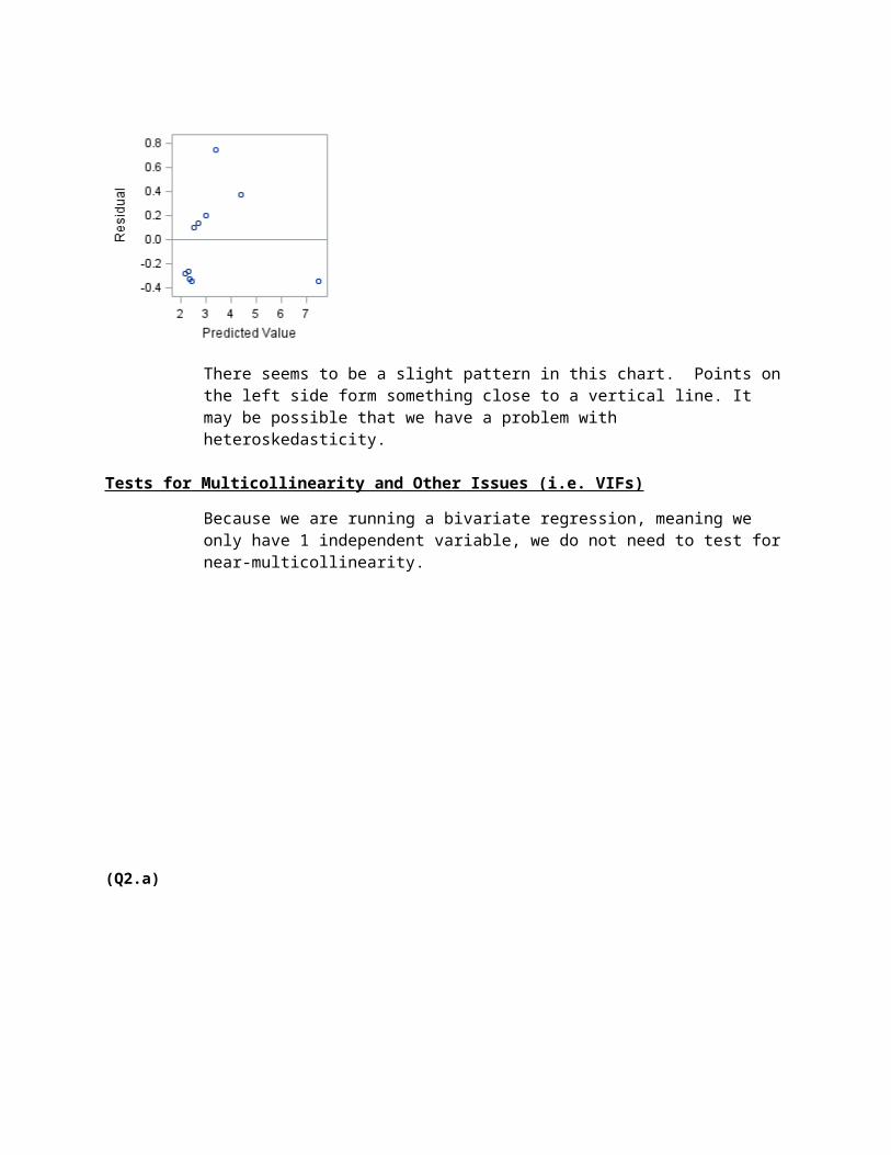
There seems to be a slight pattern in this chart. Points on the left side form something close to a vertical line. It may be possible that we have a problem with heteroskedasticity.

Tests for Multicollinearity and Other Issues (i.e. VIFs)

Because we are running a bivariate regression, meaning we only have 1 independent variable, we do not need to test for near-multicollinearity.

(Q2.a)

Regression Equation

lnY=ln ^β1+^β2 ln X2+

^β3 ln X3+u

Definitions

lnY=Output

lnX 2=Labor Input

ln X 3=Capital Input


H 0 : β1=β2=β3=0

H a :otherwise

Given an F value of 407.5, and a p-value of .001, we can reject H0 at the .05 level of significance, indicating that there is statistically significant evidence of a relationship between Output and the independent variables.


R2 = .9714. This value suggests that 97.14 percent of the variation in Output is due to

changes in the independent variables.

R2 = .9690. However we must use the adjusted R squared. This value suggests that 96.90 percent of the variation in Output is due to changes in the independent variables, after adjusting for the number of independent variables. This indicates a strong relationship.


H0: β2 = 0

H1: β2 ≠ 0

Given a t-value of 3.88 and a p-value of .0007, we can reject H0 at the .05 level of significance, indicating that there is statistically significant evidence of a relationship between Output and Labor Input holding the effects of other independent variables constant. The standard error of β2 indicates the average error in estimating β2 is .59949.

H0: β3 = 0

H1: β3 ≠ 0

Given a t-value of .85 and a p-value of .4063, we can reject H0 at the .05 level of significance, indicating that there is statistically significant evidence of a relationship between Output and Capital holding the effects of other independent variables constant. The standard error of β3 indicates the average error in estimating β3 is .16539.


β1 = -11.9366 is the intercept where the regression plane crosses the Y-axis. However, because this represents the estimated value of Output when all independent variables are equal to zero, this interpretation is reliable only when the data contains values of zero for each independent variable.

β2 = A one percent increase in Labor Input would result in a 2.3284% change in Output, holding the effects of other independent variables constant.

β3 = A one percent increase in Capital Input would result in a .13981% change in Output, holding the effects of other independent variables constant.


The standard estimates are .81107 for Labor Input and .17652 for Capital Input. The standardized regression coefficients indicate that Labor Input is contributing the greatest change/effect on our dependent variable.


The standard error of the regression indicates that the average error in predicting Y using the regression equation is .08123.


Our coefficient of variation compares the average error in predicting Y to the value of the dependent variable mean, and indicates that our model will have and average error of 1.80754% when predicting the value of our dependent variable.

Plot Interpretation

A majority of the plot points are scattered along the bottom left to bottom right, hence there is an obvious pattern. This might indicate heteroscedasticity.

a. A general conclusion one can draw is that there are high VIFs over 10 for both independent variables and a high p-value for Capital Input at .4063. Also, there is a problem with near multicollinearity in the sample regression equation.


Near multicollinearity can be detected in this regression by the high R2 value at .9714 and F value at 407.50 with the presence of low t-statistics for most of the independent variables. The variance inflation factors for each independent variable are over 10, VIF of 36.58672 for both Capital Input and Labor Input. Since the adjusted condition index is 12.014, it exceeds the threshold of 10, which indicates a severe multicollinearity problem may exist.

(Q2.2)

Regression Equation

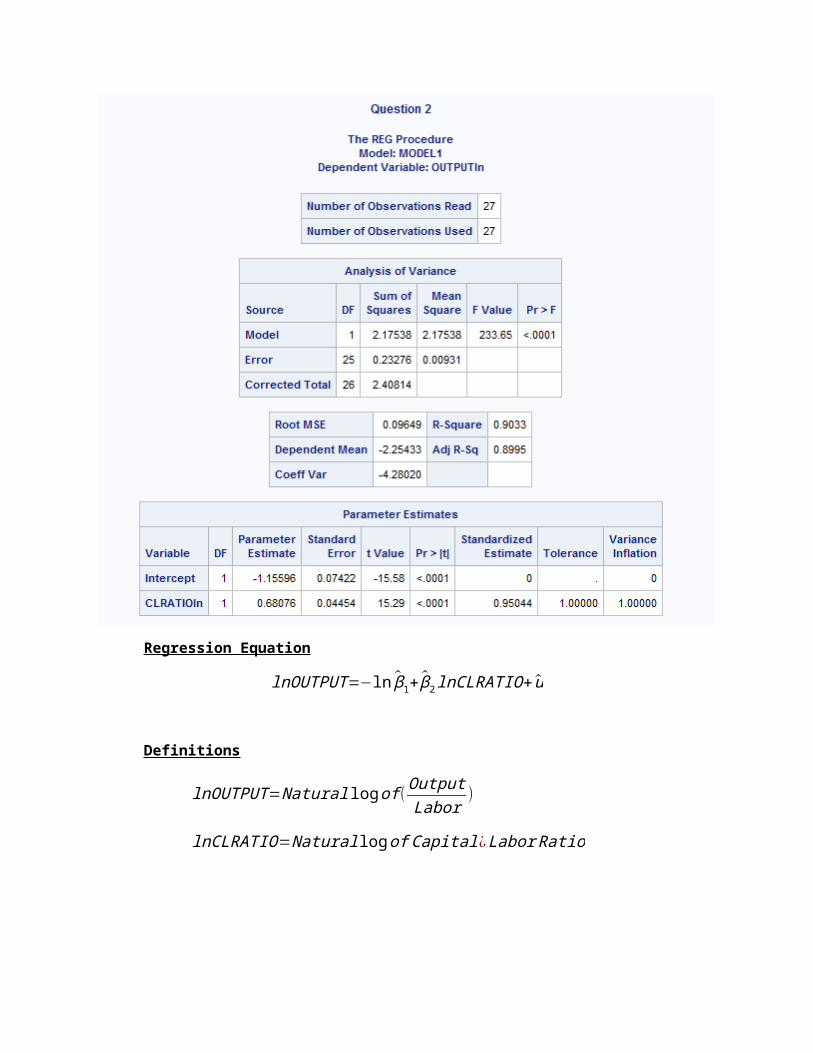
lnOUTPUT=−ln β1+ β2 lnCLRATIO+u

Definitions

lnOUTPUT=Natural log of (OutputLabor

)

lnCLRATIO=Natural log of Capital ¿Labor Ratio


H 0 : β1=β2=0

H a :otherwise

Given an F value of 233.65, and a p-value of .0001, we can reject H0 at the .05 level of significance, indicating that there is statistically significant evidence of a relationship between lnOUTPUT and the independent variable.


R2 = .9033. This value suggests that 90.33 percent of the variation in lnOUTPUT is

due to changes in the independent variable.

R2 = .8995 This value suggests that 89.95 percent of the variation in lnOUTPUT is due to changes in the independent variables, after adjusting for the number of independent variable.


H0: β2 = 0

H1: β2 ≠ 0

Given a t-value of 15.29 and a p-value of .0001, we can reject H0 at the .05 level of significance, indicating that there is statistically significant evidence of a relationship with lnOUTPUT . The standard error of β2 indicates the average error in estimating β2 is .04454.


β1 = -1.15596 is the intercept where the regression plane crosses the Y-axis. However, because this represents the estimated value of lnOUTPUT when all independent variables are equal to zero, this interpretation is reliable only when the data contains values of zero for each independent variable.

β2 = A one percent increase in lnCLRATIO would result in a .68076% change in lnOUTPUT , holding the effects of other independent variables constant.


The standard estimate is .95044 for lnCLRATIO. The standardized regression coefficients indicate that lnCLRATIO is contributing the greatest change/effect on our dependent variable.


The standard error of the regression indicates that the average error in predicting lnOUTPUT using the regression equation is .09649.


Our coefficient of variation compares the average error in predicting lnOUTPUT to the value of the dependent variable mean, and indicates that our model will have and average error of -4.28020% when predicting the value of our dependent variable.

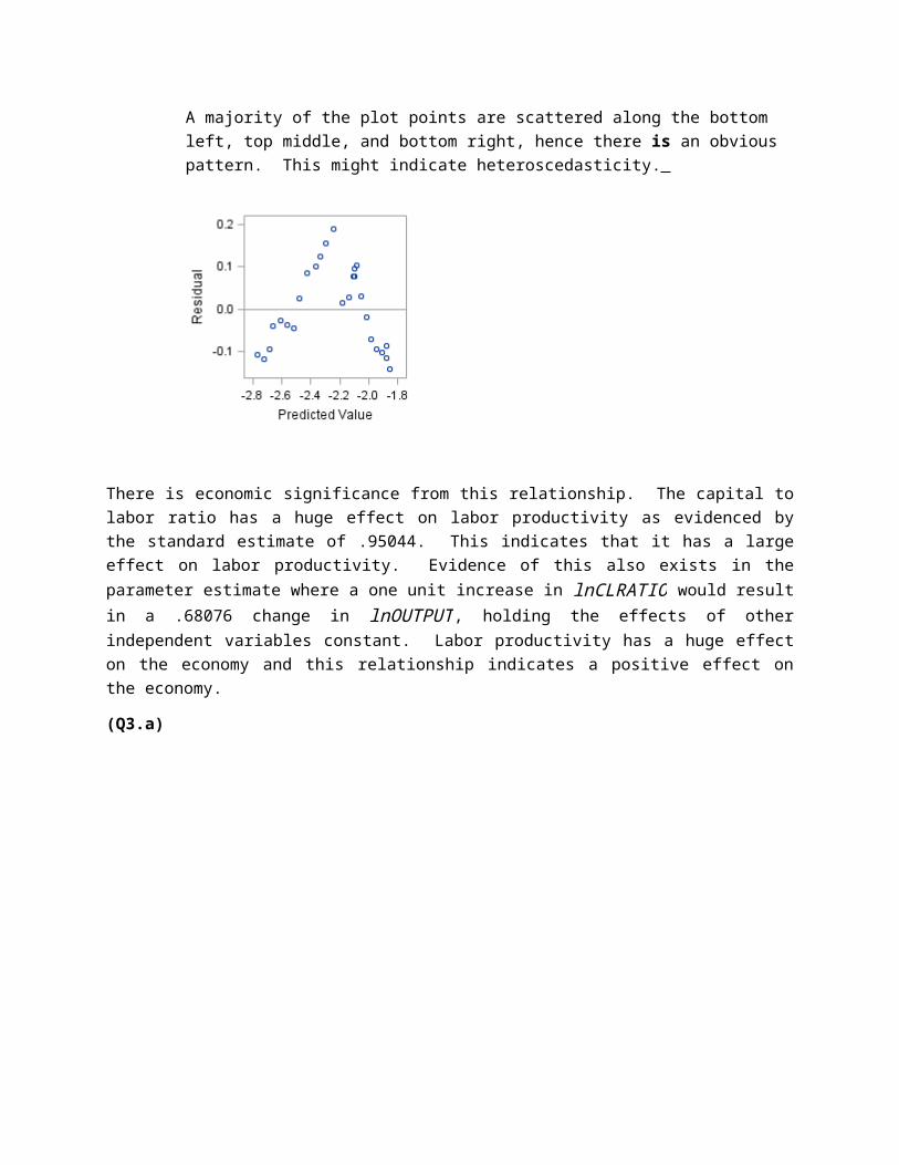
Plot Interpretation

A majority of the plot points are scattered along the bottom left, top middle, and bottom right, hence there is an obvious pattern. This might indicate heteroscedasticity.

There is economic significance from this relationship. The capital to labor ratio has a huge effect on labor productivity as evidenced by the standard estimate of .95044. This indicates that it has a large effect on labor productivity. Evidence of this also exists in the parameter estimate where a one unit increase in lnCLRATIO would result in a .68076 change in lnOUTPUT , holding the effects of other independent variables constant. Labor productivity has a huge effect on the economy and this relationship indicates a positive effect on the economy.

(Q3.a)

Regression Equation

Hours = 1,904.57758 – 93.75255 Rate + 0.00022547 ERSP – 0.21497 ERNO + 0.15721 NEIN + 0.01557 Asset – 0.34864 Age + 20.72803 DEP + 37.32563 School + u.

DefinitionsHours = average hours worked during the yearRate = average hourly wage (dollars)ERSP = average yearly earnings of spouse (dollars)ERNO = average yearly earnings of other family members (dollars)NEIN = average yearly non-earned incomeAsset = average family assets holdings (bank account, etc.) (dollars)Age = average age of respondentDEP = average number of dependents

School = average highest grade of school completed


H 0 : β1=β2=β3=β4=β5=β6=β7=β8=β9=0H 1: β1≠ β2≠ β3≠ β4≠ β5≠ β6≠β7≠ β8≠ β9≠0

Given an F value of 15.38 and a p-value of .0001, we can reject H0 at the .05 level of significance, indicating that there is statistically significant evidence of a relationship between hours and the independent variables.


R2 = 0.8256. This value suggests that 82.56% of the variation in hours is due to changes in the

independent variables. This R2 is high which indicates that this model explains most of the variation inhours.

R2 = 0.7719. This value suggests that 77.19% of the variation in hours is due to changes in the independent variables, after adjusting for the number of independent variables. This R2 is also high indicating that this model explains most of the variation in hours. We use R2 in this case because we have multiple independent variables.


H0: β2 = 0H1: β2 ≠ 0

Given a t-value of -1.99 and a p-value of 0.0574, we can reject H0 at the 0.05 level of significance, indicating that there is statistically significant evidence of a relationship between hours and rate holding the effects of other independent variables constant. The standard error of β2 indicates the average error in estimating β2 is 47.14500.

H0: β3 = 0H1: β3 ≠ 0

Given a t-value of 0.01 and a p-value of 0.9953, we cannot reject H0 at the 0.05 level of significance, indicating that there is no statistically significant evidence of a relationship between hours and ERSP holding the effects of other independent variables constant. The standard error of β3 indicates the average error in estimating β3 is 0.03825.

H0: β4 = 0H1: β4 ≠ 0

Given a t-value of -2.19 and a p-value of 0.0373, we can reject H0 at the 0.05 level of significance, indicating that there is statistically significant evidence of a relationship between hours and ERNO holding the effects of other independent variables constant. The standard error of β4 indicates the average error in estimating β4 is 0.09794.

H0: β5 = 0H1: β5 ≠ 0

Given a t-value of 0.30 and a p-value of 0.7632, we cannot reject H0 at the 0.05 level of significance, indicating that there is no statistically significant evidence of a relationship between hours and NEIN holding the effects of other independent variables constant. The standard error of β5 indicates the average error in estimating β5 is 0.51641.

H0: β6 = 0H1: β6 ≠ 0

Given a t-value of 0.61 and a p-value of 0.5452, we can reject H0 at the 0.05 level of significance, indicating that there is statistically significant evidence of a relationship between hours and asset holding the effects of other independent variables constant. The standard error of β6

indicates the average error in estimating β6 is 0.2540.

H0: β7 = 0H1: β7 ≠ 0

Given a t-value of -0.09 and a p-value of 0.9261, we cannot reject H0 at the 0.05 level of significance, indicating that there is no statistically significant evidence of a relationship between hours and ageholding the effects of other independent variables constant. The standard error of β7 indicates the average error in estimating β7 is 3.72233.

H0: β8 = 0H1: β8 ≠ 0

Given a t-value of 1.23 and a p-value of 0.2305, we can reject H0 at the 0.05 level of significance, indicating that there is statistically significant evidence of a relationship between hours and DEPholding the effects of other independent variables constant. The standard error of β 8


H0: β9 = 0H1: β9 ≠ 0

Given a t-value of 1.65 and a p-value of 0.1116, we can reject H0 at the 0.05 level of significance, indicating that there is statistically significant evidence of a relationship between hours and Schoolholding the effects of other independent variables constant. The standard error of β 9


From these results we can conclude that all independent variables except for Age, NEIN, and ERSP have a statistically significant relationship with hours.


β1 = 1904.57758 is the intercept where the regression plane crosses the Y-axis. However, because this represents the estimated value of hours when all independent variables are equal

to zero, this interpretation is reliable only when the data contains values of zero for each independent variable.

β2 = A one unit increase in rate would result in a -93.75255 change in hours, holding the effects of other independent variables constant.

β3 = A one unit increase in ERSP would result in a 0.00022547 change in hours, holding the effects of other independent variables constant.

β4 = A one unit increase in ERNO would result in a -0.21497 change in hours, holding the effects of other independent variables constant.

β5 = A one unit increase in NEIN would result in a 0.15721 change in hours, holding the effects of other independent variables constant.

β6 = A one unit increase in asset would result in a 0.01557 change in hours, holding the effects of other independent variables constant.

β7 = A one unit increase in age would result in a -0.34864 change in hours, holding the effects of other independent variables constant.

β8 = A one unit increase in DEP would result in a 20.72803 change in hours, holding the effects of other independent variables constant.

β9 = A one unit increase in school would result in a 37.32563 change in hours, holding the effects of other independent variables constant.


The standardized regression coefficients indicate that asset is contributing the greatest change/effect on our dependent variable. The standardized estimate of 0.69674 indicates a one standard deviation increase in hourshappens when there is a 0.69674 standard deviation change in asset .


The standard error of the regression indicates that the average error in predicting hours using the regression equation is 30.62279.


Our coefficient of variation compares the average error in predicting Y to the value of the dependent variable mean, and indicates that our model will have and average error of 1.43292% when predicting the value of our dependent variable. This is an extremely small value indicating a good prediction.

Plot Interpretation

There is a pattern of a cluster of points in the center and right side of the chart. This could indicate problems with heteroskedasticity.

Tests for Multicollinearity

High R2but few significant t ratios

Near multicollinearity can be detected in this regression by the high R2 value at .7719 with the presence of low t-statistics for most of the independent variables.

High pair-wise correlations among regressors

The correlation coefficients between RATE and SCHOOL have a high r value of .88127. The correlation coefficients between ASSET and NEIN have a high r value of .98751.

High VIFs

The variance inflation factors for each independent variable are over 10, VIF of 17.08235 for Rate, 180.50716 for NEIN, 192.56517 for ASSET, and 25.40177 for School.

Eigenvalues and the condition index Since the adjusted condition index is 39.3204, it exceeds the threshold of 10, which indicates a severe multicollinearity problem may exist.

Auxiliary Regressions

RATE= β1+ β2ERSP+ β3ERNO+ β4 NEIN+ β5 ASSET+ β6 AGE+ β7DEP+ β8SCHOOL+u

H0: β2 = 0

H1: β2 ≠ 0

Given a t-value of -.36 and a p-value of .7243, we cannot reject H0 at the .05 level of significance, indicating that is not statistically significant evidence of a relationship between ESRPand RATE.

NEIN= β1+ β2RATE+ β3ERSP+ β4 ERNO+ β5 ASSET+ β6 AGE+ β7DEP+ β8SCHOOL+u

All of the t-values are greater than the p-value, indicating that there is statistically significant evidence of a relationship between NEIN and all the independent variables.

ASSET= β1+ β2N EIN+ β3RATE+ β4 ERSP+ β5ERNO+ β6 AGE+ β7DEP+ β8SCHOOL+u

H0: β8 = 0

H1: β8 ≠ 0

Given a t-value of .14 and a p-value of .8888, we cannot reject H0 at the .05 level of significance, indicating that there is not statistical significant evidence of a relationship between SCHOOL and ASSET .

SCHOOL= β1+ β2NEIN+ β3RATE+ β4 ERSP+ β5ERNO+ β6 ASSET+ β7 AGE+ β8DEP+u

H0: β6 = 0

H1: β6 ≠ 0

Given a t-value of .14 and a p-value of .8888, we cannot reject H0 at the .05 level of significance, indicating that there is not statistical significant evidence of a relationship between ASSET and SCHOOL.

H0: β8 = 0

H1: β8 ≠ 0

Given a t-value of .14 and a p-value of .8863, we cannot reject H0 at the .05 level of significance, indicating that there is not statistical significant evidence of a relationship between DEP and SCHOOL.

c. Refer back to regression table.

d. If there was a multicollinearity problem the remedial actions we would take would be: use prior information where appropriate, obtain more data by increasing the sample size or pool time-series and cross-sectional data, transform variables by taking the first differences for time-series data or if multicollinearity can be traced to a specific variable divide both sides of the regression equation by this highly collinear variable, and drop or replace the problem variables.

e. This study tells me a negative income tax is feasible as long as we focus on average family asset holdings. This is evidenced by how the variable asset has the greatest effect on labor supply indicated by its standard estimate of .69674.

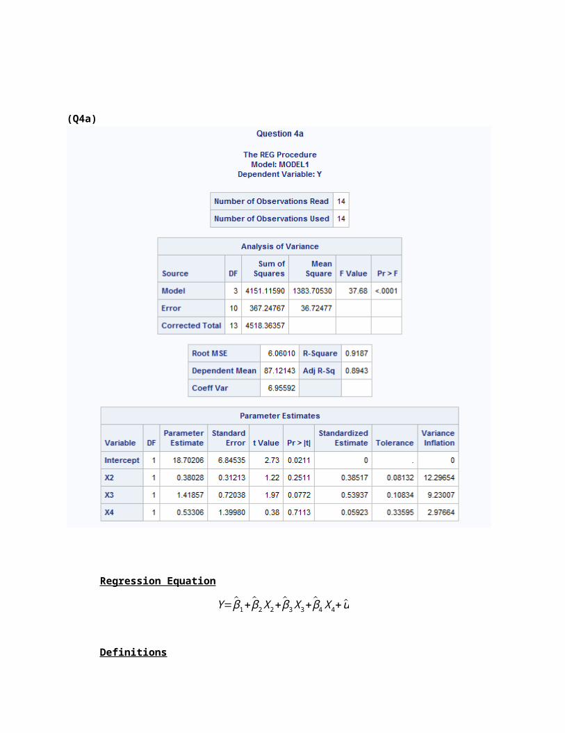
(Q4a)

Regression Equation

Y= β1+ β2 X2+ β3 X3+ β4 X 4+u

Definitions

Y=Consumption

X2=Wage Income

X3=NonwageNonfarm Income

X 4=Farm Income


H 0 : β1=β2=β3=β4=0

H a :otherwise

Given an F value of 37.68, and a p-value of .0001, we can reject H0 at the .05 level of significance, indicating that there is statistically significant evidence of a relationship between Consumption and the independent variable.


R2 = .9187. This value suggests that 91.87 percent of the variation in Consumption is

due to changes in the independent variables.

R2 = .8943 However we must use the adjusted R squared. This value suggests that 89.43 percent of the variation inConsumptionis due to changes in the independent variables, after adjusting for the number of independent variables. This indicates a strong relationship.


H0: β2 = 0

H1: β2 ≠ 0

Given a t-value of 1.22 and a p-value of .2511, we can reject H0 at the .05 level of significance, indicating that there is statistically significant evidence of a relationship between Consumption and Wage Income , holding the effects of other independent variables constant. The standard error of β2 indicates the average error in estimating β2

is .31213.

H0: β3 = 0

H1: β3 ≠ 0

Given a t-value of 1.97 and a p-value of .0772, we can reject H0 at the .05 level of significance, indicating that there is statistically significant evidence of a relationship between Consumption and NonwageNonfarm Income, holding the effects of other independent variables constant. The standard error of β3 indicates the average error in estimating β3 is .72038.

H0: β4 = 0

H1: β4 ≠ 0

Given a t-value of .38 and a p-value of .7113, we cannot reject H0 at the .05 level of significance, indicating that there is not a statistical significant evidence of a relationship between Consumption and Farm Income , holding the effects of other independent variables constant. The standard error of β3 indicates the average error in estimating β3 is 1.39980.


β1 = 18.70206 is the intercept where the regression plane crosses the Y-axis. However, because this represents the estimated value of Consumption when all independent variables are equal to zero, this interpretation is reliable only when the data contains values of zero for each independent variable.

β2 = A one unit increase in Wage Income would result in a .38028 change in Consumption, holding the effects of other independent variables constant.

β3 = A one unit increase in NonwageNonfarm Income would result in a 1.41857 change in Consumption, holding the effects of other independent variables constant.

β4 = A one unit increase in Farm Income would result in a .53306 change in Consumption, holding the effects of other independent variables constant.


The standard estimate is .38517 for Wage Income, .53937 for NonwageNonfarm Income, and .05923 for Farm Income. The standardized regression coefficients indicate that NonwageN onfarmIncome is contributing the greatest change/effect on our dependent variable.


The standard error of the regression indicates that the average error in predicting Consumption using the regression equation is 6.06010.


Our coefficient of variation compares the average error in predicting Consumption to the value of the dependent variable mean, and indicates that our model will have and average error of 6.95592% when predicting the value of our dependent variable.

Plot Interpretation

A majority of the plot points are clustered at the top right-hand corner and diagonally across the top left corner to bottom right corner, hence there is an obvious pattern. This might indicate heteroscedasticity.

Tests for Multicollinearity

High R2but few significant t ratios

Near multicollinearity can be detected in this regression by the high R2 value at .9187 with the presence of low t-statistics for most of the independent variables.

High pair-wise correlations among regressors

There is high correlation between X2 and X3 at a .94311 value, which is great than the .8 thresholds. Also, X2 and X4 have a moderate correlation at a .81070 value.

High VIFs

The variance inflation factors for each independent variable are over 10, VIF of 12.296 for X2.

Eigenvalues and the condition index

The condition index is below the threshold of 10, at a 7.41739 value.

Auxiliary Regressions

X2= β1+ β2 X3+ β3X 4

H0: β2 = 0

H1: β2 ≠ 0

Given a t-value of 5.95 and a p-value of .0001, we can reject H0 at the .05 level of significance, indicating that there is statistically significant evidence of a relationship between Wage Income and NonwageNonfarm Income.

X3= β1+ β2 X2+ β3X 4

H0: β2 = 0

H1: β2 ≠ 0

Given a t-value of 5.95 and a p-value of .0001, we can reject H0 at the .05 level of significance, indicating that there is statistically significant evidence of a relationship between NonwageNonfarm Income and Wage Income.

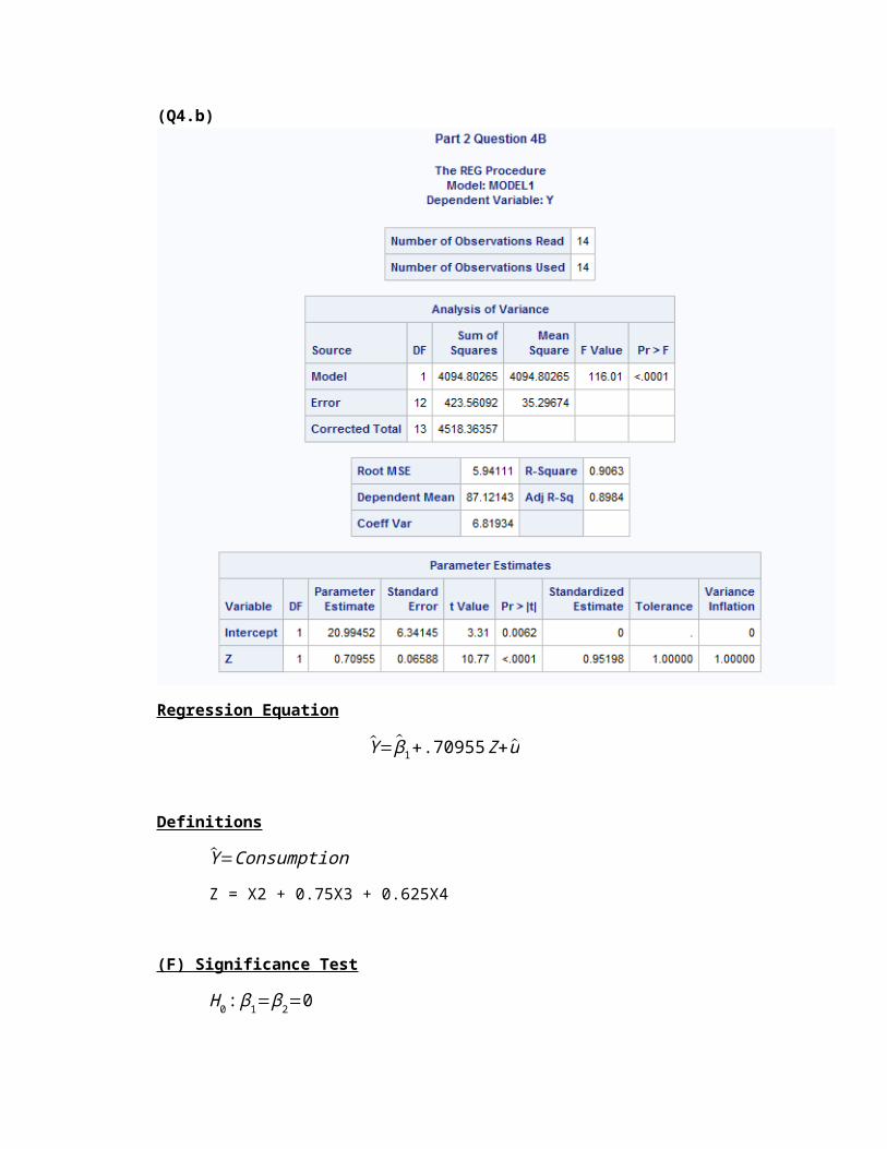
(Q4.b)

Regression Equation

Y= β1+.70955Z+u

Definitions

Y=Consumption

Z = X2 + 0.75X3 + 0.625X4


H 0 : β1=β2=0

H a :otherwise

Given an F value of 116.01, and a p-value of .0001, we can reject H0 at the .05 level of significance, indicating that there is statistically significant evidence of a relationship between Consumption and the independent variable.


R2 = 0.9063. This value suggests that 90.63% of the variation in Consumption is due to

changes in the independent variables.

R2 = 0.8984 This value suggests that 89.84% of the variation inConsumptionis due to changes in the independent variables, after adjusting for the number of independent variables. However, we do not need to use this because there is only 1 independent variable.


H0: β2 = 0

H1: β2 ≠ 0

Given a t-value of 10.77 and a p-value of .0001, we can reject H0 at the .05 level of significance, indicating that there is statistically significant evidence of a relationship betweenY and Z ,holding the effects of other independent variables constant. The standard error of β2 indicates the average error in estimating β2 is 0.06588.


β1 = 20.99452 is the intercept where the regression plane crosses the Y-axis.

However, because this represents the estimated value of Ywhen all independent variables are equal to zero, this interpretation is reliable only when the data contains values of zero for each independent variable.

β2 = A one unit increase in Z would result in a 0.70955 change in Y , holding the effects of other independent variables constant.


The standardized regression coefficients indicate that Z is contributing the greatest change/effect on our dependent variable. The standardized estimate of 0.95198 indicates a one standard deviation increase in Y happens when there is a 0.95198 standard deviation change in Z.


The standard error of the regression indicates that the average error in predicting Y using the regression equation is 5.94111.


Our coefficient of variation compares the average error in predicting Y to the value of the dependent variable mean, and indicates that our model will have and average error of 6.81934% when predicting the value of our dependent variable.

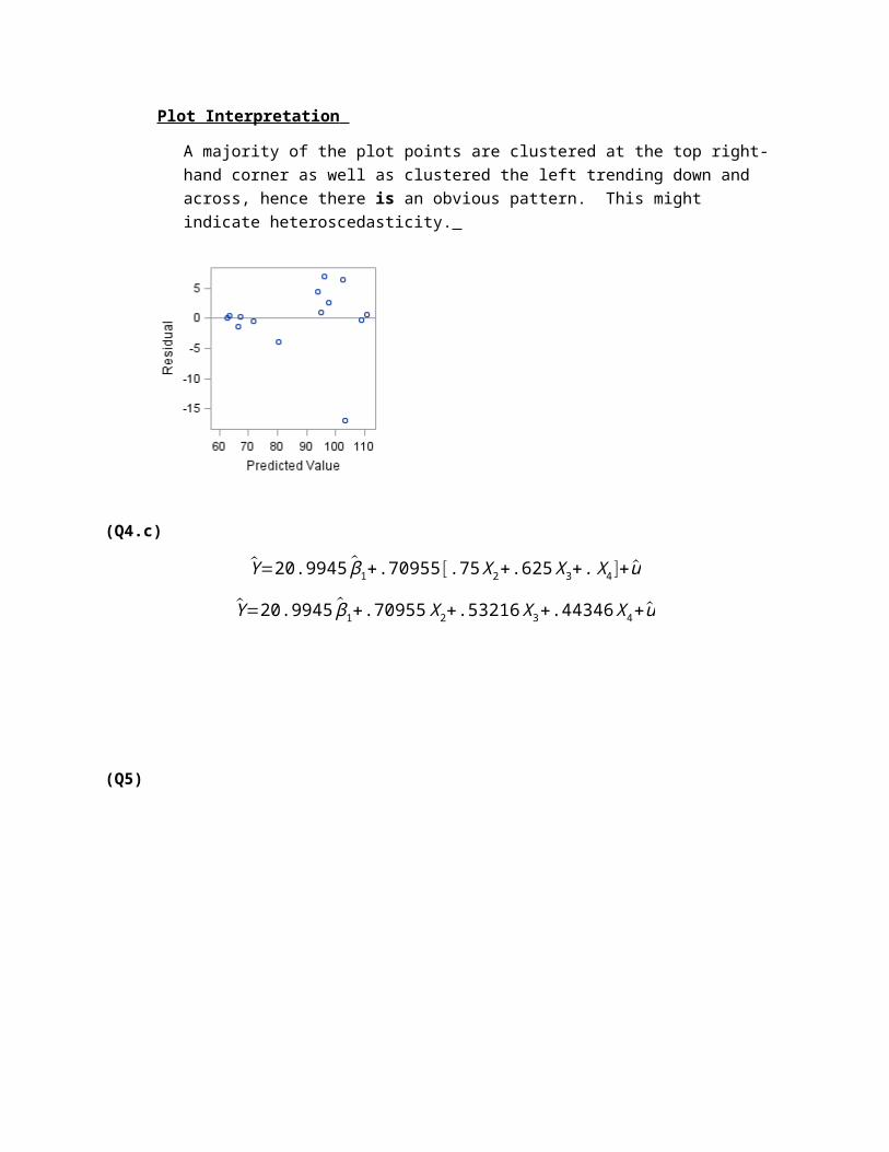
Plot Interpretation

A majority of the plot points are clustered at the top right-hand corner as well as clustered the left trending down and across, hence there is an obvious pattern. This might indicate heteroscedasticity.

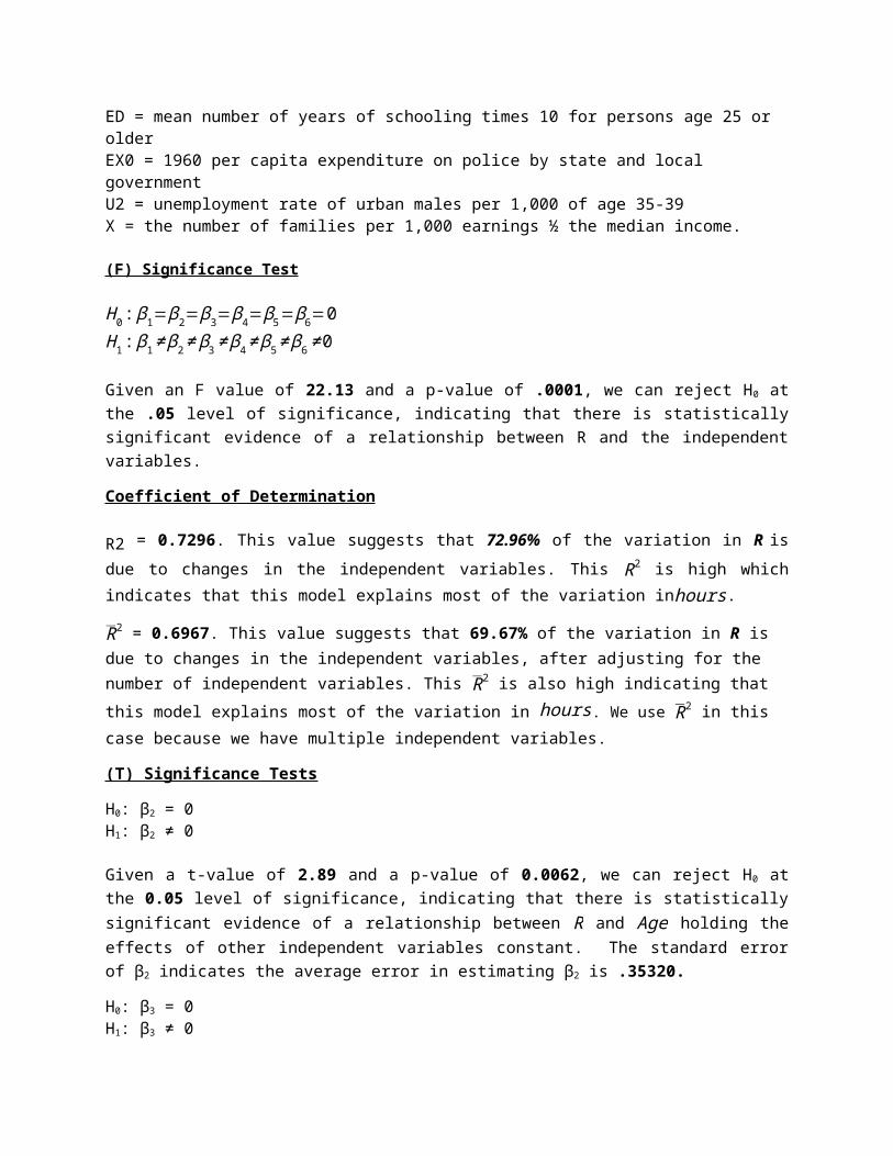
(Q4.c)

Y=20.9945 β1+.70955[ .75 X2+.625 X3+. X4 ]+u

Y=20.9945 β1+.70955 X2+.53216 X3+.44346 X4+u

(Q5)

Regression Equation

R = -524.37433 + 1.01982 Age + 2.03077 ED + 1.23312 EX0 + 0.91361 U2 + 0.63493 + u.

Definitions

R = crime rate, number of offenses reported to police per million population Age = number of males of age 14-24 per 1,000 populationED = mean number of years of schooling times 10 for persons age 25 or olderEX0 = 1960 per capita expenditure on police by state and local governmentU2 = unemployment rate of urban males per 1,000 of age 35-39X = the number of families per 1,000 earnings ½ the median income.


H 0 : β1=β2=β3=β4=β5=β6=0H 1: β1≠ β2≠ β3≠ β4≠ β5≠ β6≠0

Given an F value of 22.13 and a p-value of .0001, we can reject H0 at the .05 level of significance, indicating that there is statistically significant evidence of a relationship between R and the independent variables.


R2 = 0.7296. This value suggests that 72.96% of the variation in R is due to changes in the independent

variables. This R2 is high which indicates that this model explains most of the variation inhours.

R2 = 0.6967. This value suggests that 69.67% of the variation in R is due to changes in the independent variables, after adjusting for the number of independent variables. This R2 is also high indicating that this model explains most of the variation in hours. We use R2 in this case because we have multiple independent variables.


H0: β2 = 0H1: β2 ≠ 0

Given a t-value of 2.89 and a p-value of 0.0062, we can reject H0 at the 0.05 level of significance, indicating that there is statistically significant evidence of a relationship between R and Age holding the effects of other independent variables constant. The standard error of β2 indicates the average error in estimating β2 is .35320.

H0: β3 = 0H1: β3 ≠ 0

Given a t-value of 4.28 and a p-value of 0.0001, we can reject H0 at the 0.05 level of significance, indicating that there is statistically significant evidence of a relationship between R and ED holding the effects of other independent variables constant. The standard error of β3 indicates the average error in estimating β3 is 0.47419.

H0: β4 = 0H1: β4 ≠ 0

Given a t-value of 8.71 and a p-value of 0.0001, we can reject H0 at the 0.05 level of significance, indicating that there is statistically significant evidence of a relationship between R and EX 0 holding the effects of other independent variables constant. The standard error of β4 indicates the average error in estimating β4 is 0.14163.

H0: β5 = 0H1: β5 ≠ 0

Given a t-value of 2.10 and a p-value of 0.0415, we can reject H0 at the 0.05 level of significance, indicating that there is statistically significant evidence of a relationship between R and U 2 holding the effects of other independent variables constant. The standard error of β5 indicates the average error in estimating β5 is 0.43409.

H0: β6 = 0H1: β6 ≠ 0

Given a t-value of 4.32 and a p-value of 0.0001, we can reject H0 at the 0.05 level of significance, indicating that there is statistically significant evidence of a relationship between R and X holding the effects of other independent variables constant. The standard error of β6 indicates the average error in estimating β6 is 0.14685.

From these results we can conclude that all the independent variables have a statistically significant relationship with R.


β1 = -524.37433 is the intercept where the regression plane crosses the Y-axis. However, because this represents the estimated value of R when all independent variables are equal to zero, this interpretation is reliable only when the data contains values of zero for each independent variable.

β2 = A one unit increase in Age would result in a 1.01982 change in R, holding the effects of other independent variables constant.

β3 = A one unit increase in ED would result in a 2.03077 change in R, holding the effects of other independent variables constant.

β4 = A one unit increase in EX0 would result in a 1.23312 change in R, holding the effects of other independent variables constant.

β5 = A one unit increase in U2 would result in a 0.91361 change in R, holding the effects of other independent variables constant.

β6 = A one unit increase in X would result in a 0.63493 change in R, holding the effects of other independent variables constant.


The standardized regression coefficients indicate that EX 0 is contributing the greatest change/effect on our dependent variable. The standardized estimate of 0.94754 indicates a one standard deviation increase in Rhappens when there is a 0.94754 standard deviation change in EX 0.


The standard error of the regression indicates that the average error in predicting R using the regression equation is 21.31035.


Our coefficient of variation compares the average error in predicting Y to the value of the dependent variable mean, and indicates that our model will have and average error of 23.53519% when predicting the value of our dependent variable. This is an small value indicating a good prediction.

Plot Interpretation

There is a pattern showing a cluster of points near the center of the chart indicating a possible problem with heteroskedasticity.

The condition index is at 3.79332 along with no VIF over 10, there is strong indication that there is little multicollinearity if any. However, in the original model we found multicollinearity, which the

independent variable EX1 effected the model so we first took EX1 followed by the variables with high VIFS over 10 as well as high correlations over .8 value.

(Q6.a)

Regression Equation

ln Imports = 1.40942 + 1.85010 GDPln – 0.87337 CPIln +u.

Definitions

Imports = Imports for the United States over the period 1975-2005. GDPln = log of GDP

CPIln = log of CPI


H 0 : β1=β2=β3=0H 1: β1≠ β2≠ β3≠0

Given an F value of 1737.19 and a p-value of .0001, we can reject H0 at the .05 level of significance, indicating that there is statistically significant evidence of a relationship between Imports and the independent variables.


R2 = 0.9920. This value suggests that 99.20% of the variation in Imports is due to changes in the

independent variables. This R2 is very high which indicates that this model explains almost all of the variation inImports.

R2 = 0.9914. This value suggests that 99.14% of the variation in Imports is due to changes in the independent variables, after adjusting for the number of independent variables. This R2 is also high indicating that this model explains most of the variation in Imports. We use R2 in this case because we have multiple independent variables.


H0: β2 = 0H1: β2 ≠ 0

Given a t-value of 10.11 and a p-value of 0.0001, we can reject H0 at the 0.05 level of significance, indicating that there is statistically significant evidence of a relationship between Imports and GDPln holding the effects of other independent variables constant. The standard error of β 2 indicates the average error in estimating β2 is 0.18291.

H0: β3 = 0H1: β3 ≠ 0

Given a t-value of -3.07 and a p-value of 0.0048, we can reject H0 at the 0.05 level of significance, indicating that there is statistically significant evidence of a relationship between Imports and CPIlnholding the effects of other independent variables constant. The standard error of β 3 indicates the average error in estimating β3 is 0.28481.

From these results we can conclude that all the independent variables have a statistically significant relationship with Imports.


β1 = 1.40942 is the intercept where the regression plane crosses the Y-axis. However, because this represents the estimated value of Imports when all independent variables are equal to zero, this interpretation is reliable only when the data contains values of zero for each independent variable.

β2 = A one percent increase in GDPln would result in a 1.85010% change in Imports, holding the effects of other independent variables constant.

β3 = A one percent increase in CPIln would result in a – 0.87337% change in Imports, holding the effects of other independent variables constant.


The standardized regression coefficients indicate that GDPln is contributing the greatest change/effect on our dependent variable. The standardized estimate of 1.42292 indicates a one standard deviation increase in Importshappens when there is a 0.95582 standard deviation change in GDPln.





Plot Interpretation

There is an obvious pattern where points rise and fall indicating we may have a problem with heteroskedasticity.

b. I do suspect that there is multicollinearity in the data due to a high r squared and low t-values as well as VIFs well over 10.

(Q6.c)


H0: β2 = 0H1: β2 ≠ 0

Given a t-value of 51.83 and a p-value of 0.0001, we can reject H0 at the 0.05 level of significance, indicating that there is statistically significant evidence of a relationship between Imports and GDPln holding the effects of other independent variables constant. The standard error of β 2 indicates the average error in estimating β2 is 0.02495.

Plot Interpretation

There is an obvious pattern where points rise and fall throughout the chart indicating we may have a problem with heteroskedasticity.

c2.


H0: β3 = 0H1: β3 ≠ 0

Given a t-value of 27.39 and a p-value of 0.0001, we can reject H0 at the 0.05 level of significance, indicating that there is statistically significant evidence of a relationship between Imports and CPIln holding the effects of other independent variables constant. The standard error of β 3 indicates the average error in estimating β3 is 0.07251.

Plot Interpretation

There is an obvious pattern where the points rise and fall throughout the chart indicating we may have a problem with heteroskedasticity.

c3.


H0: β3 = 0H1: β3 ≠ 0

Given a t-value of 44.51 and a p-value of 0.0001, we can reject H0 at the 0.05 level of significance, indicating that there is statistically significant evidence of a relationship between Imports and CPIln holding the effects of other independent variables constant. The standard error of β 3 indicates the average error in estimating β3 is 0.0.03473.

Plot Interpretation

There appears to be an obvious pattern where the points rise and fall throughout the chart indicating we may have a problem with heteroskedasticity.

Even though near multicollinearity may be a problem, we cannot discard either independent variable because all are significant in the auxiliary regressions. If we discard an independent model then our model may become an incomplete model.

(Q7)

(Q7.a)

*Question 7;Title "Question 7";PROC IMPORT datafile="I:\SASV507\Homeworkdatasets\Homework2\Indiana Sales I.xls"

Out=V507.SalesIDbms=xls;getnames=yes;

RUN;

PROC IMPORT datafile="I:\SASV507\Homeworkdatasets\Homework2\Indiana Sales IIb.xls"

Out=V507.SalesIIbDbms=xls;getnames=yes;

RUN;

PROC SORT data=V507.SalesI;BY Calyear;

RUN;

PROC SORT data=V507.SalesIIb;BY Calyear;

RUN;

DATA V507.salesmerge;MERGE V507.salesI v507.salesIIb;BY Calyear;

RUN;

(Q7.b)

DATA V507.salesmerge2;SET V507.salesmerge;Salesbsln = LOG(SalesBase);PIPCAP = Income/Pop;

RUN;

(Q7.c)

DATA V507.salesmerge3;SET V507.salesmerge2;IF QTR>3 THEN QTR4=1;ELSE QTR4=0;

RUN;

(Q7.d)

PROC REG DATA=V507.salesmerge3;MODEL Salesbsln = PIPCAP QTR4 HPI unemprate/stb vif tol collin collinoint;RUN;

(Q7.e)

Regression Equation

Tax Base = 9.15914 + 28.61509 PIPCAP – 0.04963 QTR4 – 0.00227 HPI – 0.01479 UnempRate + u.

Definitions

Tax Base = Indiana Sales Tax Base PIPCAP = Personal Income Per Capita

QTR4 = 4th quarter of calendar yearHPI = House Price IndexUnempRate = Indiana Unemployment Rate


H 0 : β1=β2=β3=β4=β5=0H 1: β1≠ β2≠ β3≠ β4≠ β5≠0

Given an F value of 40.42 and a p-value of .0001, we can reject H0 at the .05 level of significance, indicating that there is statistically significant evidence of a relationship between Tax Base and the independent variables.


R2 = 0.8996. This value suggests that 89.96% of the variation in Tax Base is due to changes in the

independent variables. This R2 is high which indicates that this model explains most of the variation inTaxBase.

R2 = 0.8775. This value suggests that 87.75% of the variation in Tax Base is due to changes in the independent variables, after adjusting for the number of independent variables. This R2 is also high indicating that this model explains most of the variation in TaxBase . We use R2 in this case because we have multiple independent variables.


H0: β2 = 0H1: β2 ≠ 0

Given a t-value of 9.09 and a p-value of 0.0001, we can reject H0 at the 0.05 level of significance, indicating that there is statistically significant evidence of a relationship between TaxBase and PIPCAP holding the effects of other independent variables constant. The standard error of β 2


H0: β3 = 0H1: β3 ≠ 0

Given a t-value of -4.78 and a p-value of 0.0001, we can reject H0 at the 0.05 level of significance, indicating that there is statistically significant evidence of a relationship between TaxBase and QTR 4holding the effects of other independent variables constant. The standard error of β 3 indicates the average error in estimating β3 is 0.01038.

H0: β4 = 0H1: β4 ≠ 0

Given a t-value of -0.80 and a p-value of 0.4363, we can reject H0 at the 0.05 level of significance, indicating that there is statistically significant evidence of a relationship between TaxBase and HPI holding the effects of other independent variables constant. The standard error of β 4 indicates the average error in estimating β4 is 0.00285.

H0: β5 = 0H1: β5 ≠ 0

Given a t-value of -7.34 and a p-value of 0.0001, we can reject H0 at the 0.05 level of significance, indicating that there is statistically significant evidence of a relationship between TaxBase and

UnempRate holding the effects of other independent variables constant. The standard error of β 5


From these results we can conclude that all the independent variables have a statistically significant relationship with Tax Base.


β1 = 9.15914 is the intercept where the regression plane crosses the Y-axis. However, because this represents the estimated value of Tax Base when all independent variables are equal to zero, this interpretation is reliable only when the data contains values of zero for each independent variable.

β2 = A one unit increase in PIPCAP would result in a 2861.509% change in Tax Base, holding the effects of other independent variables constant.

β3 = A one unit increase in QTR4 would result in a – 4.963% change in Tax Base, holding the effects of other independent variables constant.

β4 = A one unit increase in HPI would result in a – .227% change in Tax Base, holding the effects of other independent variables constant.

β5 = A one unit increase in UnempRate would result in a – 1.479% change in Tax Base, holding the effects of other independent variables constant.


The standardized regression coefficients indicate that PIPCAP is contributing the greatest change/effect on our dependent variable. The standardized estimate of 0.95582 indicates a one standard deviation increase in TaxBasehappens when there is a 0.95582 standard deviation change in PIPCAP.





Plot Interpretation

There seems to be an obvious pattern of a vertical line of points on the right side of the chart as well as a cluster of points in the center of the chart. This indicates that we may have a problem with heteroskedasticity.


Multicollinearity is not a concern because all of the VIFs are at 1 and the CI is under 10.

(Q7.f) The data is not consistent with this assertion because HPI has a negative effect on tax revenue as evidence by its parameter estimate of -0.00227, its t-value of -7.34, and its standard estimate of -0.08082. A one unit increase in HPI would result in a – 0.00227 change in Tax Base, holding the effects of other independent variables constant. As you can see increasing HPI causes a loss in tax revenue therefore the politician is wrong.

(Q7.g) The best way to increase sales tax revenues base on the regression results is to maintained personal income per capita. According to the regression results a one unit increase in PIPCAP would result in a 2861.509% change in Tax Base, holding the effects of other independent variables constant. Finding ways to increase the employment rate could raise personal income within the population. Currently in the regression results, for every one unit increase in UnempRate would result in a – 1.479% change in Tax Base, holding the effects of other independent variables constant. Therefore, the Governor could elect for more educational programs and vocational programs, which could decrease

unemployment rate bringing more citizens into the workforce thus increasing sales tax revenues. I would suggest the Governor to analyze the benefit-cost for educational, vocational, and training programs with unemployment rate.

hines.buckler-homework2final

Documents