MNRAS 000, 1–42 (2017) Preprint 2 August 2019 Compiled using MNRAS LATEX style file v3.0

HISS, a new tool for H i stacking: application to NIBLESspectra

J. Healy,1,2? S-L. Blyth,1 E. Elson,1,3 W. van Driel,4,5 Z. Butcher,6 S. Schneider,6

M.D. Lehnert,7 and R. Minchin8,91Department of Astronomy, University of Cape Town, Private Bag X3, Rondebosch 7701, South Africa2Kapteyn Astronomical Institute, University of Groningen, Landleven 12, 9747 AV Groningen, The Netherlands3Department of Physics and Astronomy, University of the Western Cape, Robert Sobukwe Road, Bellville, 7535, South Africa4GEPI, Observatoire de Paris, PSL Research University, CNRS, 5 place Jules Janssen, 92190 Meudon, France5Station de Radioastronomie de Nancay, Observatoire de Paris, CNRS/INSU USR 704, Universite d’Orleans OSUC, route de Souesmes,

18330 Nancay, France6University of Massachusetts, Astronomy Program, 619E LGRT-B, Amherst, MA 01003, U.S.A.7Sorbonne Universite, CNRS UMR 7095, Institut d’Astrophysique de Paris, 98bis bd Arago, 75014 Paris, France8Arecibo Observatory, National Astronomy and Ionosphere Center, Arecibo, PR 00612, USA9SOFIA-USRA, NASA Ames Research Center, MS 232-12, Moffett Field, CA 94035, USA

Accepted XXX. Received YYY; in original form ZZZ

ABSTRACTH i stacking has proven to be a highly effective tool to statistically analyse average H iproperties for samples of galaxies which may or may not be directly detected. Withthe plethora of H i data expected from the various upcoming H i surveys with theSKA Precursor and Pathfinder telescopes, it will be helpful to standardize the way inwhich stacking analyses are conducted. In this work we present a new python-basedpackage, HISS, designed to stack H i (emission and absorption) spectra in a consistentand reliable manner. As an example, we use HISS to study the H i content in variousgalaxy sub-samples from the NIBLES survey of SDSS galaxies which were selected torepresent their entire range in total stellar mass without a prior colour selection. Thisallowed us to compare the galaxy colour to average H i content in both detected andnon-detected galaxies. Our sample, with a stellar mass range of 108 < M? (M) < 1012,has enabled us to probe the H i-to-stellar mass gas fraction relationship more than halfan order of magnitude lower than in previous stacking studies.

Key words: galaxies: evolution – methods: data analysis – galaxies: ISM

1 INTRODUCTION

How galaxies evolve over cosmic time is currently a keyarea of research in astrophysics. A great deal is alreadyknown about the evolution of the stellar content of galax-ies due to recent infrared (Spitzer, Werner et al. 2004),optical (Sloan Digital Sky Survey, York et al. 2000),and ultraviolet (Galaxy Evolution Explorer, Bianchi &GALEX Team 2000) surveys. However, comparativelylittle is known about the evolution of the gas in galaxies.Understanding how the cold gas evolves is important asit is the raw fuel for the formation of stars and thus galaxies.

Neutral atomic hydrogen (H i) forms the most signifi-cant reservoir of neutral gas in galaxies. Studies have shownthat blue, star-forming galaxies have a higher fraction of

? E-mail: julia@ast.uct.ac.za

H i gas compared to red, quiescent galaxies (e.g. Roberts &Haynes 1994; Gavazzi et al. 1996; McGaugh & de Blok 1997;Cortese et al. 2011; Fabello et al. 2011; Brown et al. 2015),which suggests that H i plays an important role in starformation. H i is difficult to detect in most galaxies beyondthe local universe (z ∼ 0.06) with existing radio telescopesdue to the weak nature of the emission. Researchers havehad to exploit different techniques in order to measurevery weak H i signals from galaxies. One such technique isH i stacking; with this technique, an average H i mass pergalaxy can be estimated by co-adding the H i spectra of asample of galaxies in which H i is not necessarily directlydetected.

The idea of co-adding the undetected H i spectra instudies of the gas content in galaxies was first presentedby Zwaan et al. (2001) and Chengalur et al. (2001). Bothgroups were studying the H i within galaxies located in and

© 2017 The Authors

arX

iv:1

908.

0051

7v1

[as

tro-

ph.G

A]

1 A

ug 2

019

2 J. Healy et al.

around clusters. With low detection counts in their samples,both groups independently co-added the non-detectionsin an effort to obtain a statistically meaningful averageddetection for their samples.

Stacking analyses have become commonplace in the last15+ years. The technique has been applied in various areas:H i content of galaxies in dense environments and how thegas content relates to other observables (Chengalur et al.2001; Verheijen et al. 2007; Lah et al. 2009; Jaffe et al. 2016);gas content of active galaxies (Gereb et al. 2013, 2015);measurement of Ω at low to intermediate (z < 0.4) redshifts(Lah et al. 2007; Delhaize et al. 2013; Rhee et al. 2013,2016); and using stacking to study the relations between H iand various stellar mass/star formation indicators (Fabelloet al. 2011, 2012; Brown et al. 2015, 2017; Gereb et al. 2015).

The gas scaling relations for galaxies are averagetrends which relate the H i mass (MHi) or H i mass tostellar mass (M?) ratio (gas fraction, fHi) to various othergalaxy properties. Stacking a sample of ∼5000 galaxieswith M? > 1010 M that had both ultraviolet and opticalimaging, Fabello et al. (2011) found using H i stacking thatthe gas fraction correlates better with NUV − r colour thanstellar mass. This result was later confirmed and extendedto a sample with M? > 109 M by Brown et al. (2015).To date, studies of the H i gas scaling relations have beenlimited to samples with M? > 109 M, a mass which hasbeen identified as a turning point around which the MHi

vs M? slope changes (Huang et al. 2012; Maddox et al. 2015).

Directly detecting H i with current radio telescopesbeyond z ∼ 0.1 is challenging due to the long observingtimes required (e.g. HIGHz (Catinella & Cortese 2015) onArecibo using > 300 hours and CHILES (Fernandez et al.2016; Hess et al. 2018) on the JVLA requiring ∼ 1000 hoursof observing time). The upcoming surveys with the SKAPrecursors and Pathfinders (e.g. MeerKAT, Booth et al.2009; ASKAP, Johnston et al. 2008; APERTIF, Verheijenet al. 2008) will greatly extend the redshift range overwhich H i in galaxies is studied, either directly or indirectly.Techniques such as H i stacking will have an importantrole to play in order to study the average H i propertiesof different galaxy samples, particularly at higher redshifts(z & 0.6). Deep SKA Precursor surveys such as LADUMA1

(Holwerda et al. 2011) on MeerKAT have identified stackingas an important tool to probe higher redshifts, and push tolower H i mass limits.

As we rapidly approach the start of the PrecursorSurveys, work is under-way on developing a data analysistoolkit that will enable consistent and comparable studiesof the survey data. Already available is the versatile sourcefinder, SoFiA (Serra et al. 2015). With the importantrole that stacking will play in the analysis of high redshiftand low mass samples, it is imperative that a tool capableof reliably and consistently stacking H i spectra is developed.

In this work, we present our new software pack-

1 Looking At the Distant Universe with the MeerKAT Array

age, HISS, that has been designed for the astron-omy community in response to the need for a stack-ing software package. HISS can be downloaded fromhttps://github.com/healytwin1/HISS. We use HISS torevisit the gas scaling relations with a sample of 1000galaxies from the Nancay Interstellar Baryon Legacy Extra-galactic Survey (NIBLES van Driel et al. 2016). NIBLESis an SDSS-selected targeted H i survey with the NancayRadio Telescope which aims to study the H i properties ofgalaxies as a function stellar mass, covering a representableM? range of the ensemble of galaxies in the nearby Universe.

The outline for this paper is as follows: the first half ofthe paper (Section 2) describes the design of the H i StackingSoftware (HISS). In the second half of the paper (Section 3and Section 4), we give an introduction to the NIBLES Sur-vey and the ancillary data we use in our stacking analysisand describe the classification of H i non-detections. We usethe NIBLES sample to explore the well-known H i mass tostellar mass scaling relations in Section 4, and finally, sum-marise our findings in Section 5.

2 THE H I STACKING SOFTWARE (HISS)

The stacking method that the software needs to implementcan be summarized by the following steps:

(i) Ingest 1D 21 cm H i spectra (radio data) and list ofassociated redshifts for the sample of galaxies to bestacked;

(ii) Spectrally shift and re-scale the H i spectra to alignthe expected line emission at a common frequency(usually the H i rest frequency: 1420.4058 MHz);

(iii) Weight the spectra (according to a preferred weight-ing scheme) and co-add the spectra.

We have designed and created the H i Stacking Software(HISS) package, after discussion with colleagues and withthe following guiding principles in mind:

• be freely available in most operating systems• to be open source• easy to modify (extensible)• stack hundreds or thousands of galaxy spectra in an

efficient and reliable manner.

The Python2 programming language was chosen fordevelopment of HISS because it is freely available, can beused on any operating system, and is also one of the mostcommonly used languages within the astronomy community.Where appropriate, HISS makes use of the publicly availablePython modules (such as AstroPy, NumPy, SciPy, etc.)which have been optimized for data input, manipulation,and display.

Fig. 1 shows a flow diagram of how the processes re-quired to create a stacked spectrum are incorporated in thedifferent modules of HISS. In the sections that follow we willillustrate how each of the processes highlighted in Fig. 1 areimplemented. Basic instructions on how to run HISS can befound in Appendix A1.

2 Developed in Python 2.7, but compatible with Python 3

MNRAS 000, 1–42 (2017)

NIBLES III: Stacking 3

Start

Input Module (§ 2.2)Config File

(§ 2.2)CatalogueFile (§ 2.2)

User input point 1

BinCatalogue?

(§ 2.2)Bin Module

Stack Module (§ 2.3)

1. Select catalogue of H i spectra (§ 2.3.1)2. Convert spectra to rest-frame (§ 2.3.2)3. Co-add spectra (§ 2.3.4)

Spectra

Analysis Module (§ 2.4)

• Calculate profile detection statistics (§ 2.4.1)• Manipulate stacked spectrum (§ 2.4.2)• Characterise stacked profile (§ 2.4.3)• Calculate uncertainty (§ 2.4.4)• Save results (§ 2.5)

Uncertainty Module (§ 2.4.4)

StackingOutput

DisplayData?(§ 2.6)

User input point 2

Display Module (§ 2.6)

Stop

no

yes

no

yes

Figure 1: This flow diagram shows how the individual spectra and user information are taken by HISS to produce a stackedspectrum from which average galaxy properties (such as total H i mass, MHi, and the H i-to-stellar mass ratio, fHi) may beextracted. The orange rectangles show the six modules of the package, the blue parallelograms show the points of input oroutput, and the green diamonds show where the user may choose to incorporate the optional modules.

MNRAS 000, 1–42 (2017)

4 J. Healy et al.

2.1 Simulated Data

When developing new data analysis tools, one of the mostimportant steps is to quantify the accuracy and reliabilityof any generated results. For this purpose, simulated spec-tra are used instead of real spectra because properties ofthe input data are then well known. In this work, we usea data set of 1000 simulated H i profiles of galaxies to il-lustrate and test the capabilities of HISS. The simulatedH i spectra are created using the formulation outlined inObreschkow et al. (2009c, Appendix A), and are based onthe evaluated properties extracted from the S3-SAX cata-logue (Obreschkow et al. 2009a,b,c) for galaxies in a redshiftrange of 0.1 < z < 0.2 with a channel width of 7 km s−1 andGaussian noise of 16 µJy per channel.

2.2 Catalogue of H i spectra

When initiated, HISS requires some information about thesample of H i spectra – see Fig. 2 for an overview. The InputModule requires two input files: a configuration file and acatalogue file. There are two ways to provide HISS withthe required information: the user can provide a text filein JSON3 format or use the graphical user interface shownin Fig. 2 to generate a configuration file (also in JSONformat). The JSON format is used for the configuration fileas it is easy to read/write, and when imported into Python,the information is dumped into an easy - to - access Pythondictionary. The configuration file includes options such asdifferent weighting functions for the stacking procedure,and options to bin the stacking sample based on additionaldata provided in the catalogue file.

The catalogue file is a user-created text file in CSV4

format that contains at least the following columns,

• Object ID• Spectrum filename• Redshift• Redshift uncertainty• Other data (optional)

for each spectrum that the user would like to include in thestack. Although the catalogue file may contain any numberof columns, the non-optional columns mentioned above arethose that are required to run HISS. Additional columnscontaining numerical information such as stellar mass oroptical colour may be used to refine the catalogue into anumber of different sub-samples to be stacked separately.This refining is done through the Bin Module (Fig. 1). Inthis first version of HISS, bins can only be created usingone quantity, e.g. stellar mass or colour, and the stackedresults are stored for each sub-sample5.

During the processing of the configuration file, the code

3 JSON stands for JavaScript Object Notation, a JSON format-

ted file has the extension .json4 comma separated values5 In the current implementation this process is sequential i.e. eachbinned sub-sample of spectra is stacked one after the other. This

process will be parallelised in future versions.

checks that the catalogue file and location of the spectraexist. If these checks are passed, HISS will continue.

2.3 Stacking the spectra

The stacking procedure is the heart of HISS, and is con-trolled by the Stack Module which is responsible for read-ing in and preparing each spectrum for stacking, as well asmaintaining the stacked spectrum and associated informa-tion (e.g.,number of objects in the stack, stacked noise). Oneof the features of this module is the option that allows theuser to watch the progress of the stacking in a window suchas the one in Fig. A1. The progress window shows each ofthe spectra in the observed frame as they are read in, aswell as the individual spectra as they are converted to therest-frame and then added to the total stacked spectrum.

2.3.1 Reading in the spectra

Regardless of how the H i spectra were created, HISSrequires that the spectra be in a text file type formatcontaining a column for the spectral axis (either frequencyor velocity) and another for the flux density (in units ofµJy, mJy, Jy or flux density/beam).

Fig. A2 shows a selection of ten of the 1000 simulatedH i profiles that will be used to illustrate the different partsof HISS. Each of these have had 16 µJy Gaussian noiseadded, so as to simulate the spectra that are anticipatedfrom the deep LADUMA survey.

As each spectrum is read into HISS, it is put through aseries of quality checks:

• The spectrum’s channel width is checked to ensure itis within 5% of the entered channel width. A warningis raised if the spectrum channel width is 5% − 10%different. If the channel width is more than 10% dif-ferent the spectrum is discarded.• The input object contains the minimum and maxi-

mum redshift values for the sample of galaxies. Thischeck makes sure that the redshift associated withthe spectrum falls within these bounds.• If the user has decided to stack the spectra in units

of gas fraction, the catalogue will be checked for anassociated stellar mass value.• The final check is for spectrum length. A galaxy

mask is created based on the expected maximumwidth galaxy width for the sample. Every spectrumis checked to ensure that it has more channels thanthe length of mask. An example of a spectrum thatwould fail such a check is shown in the panel (j) ofFig. A2 and Fig. A3.

Due to the discrete nature of the input spectra, thechannel width check is important to avoid co-adding arrayswhere the rest-frame size of the channel (i.e velocity widthin km s−1) changes significantly (> 10%) between differentarrays. The spectra that do not pass at least one of thequality checks are excluded from the stack. The object IDsfor the excluded spectra and the reason for exclusion arerecorded in the log file.

MNRAS 000, 1–42 (2017)

NIBLES III: Stacking 5

Figure 2: Screen shot from GUI main window, useful for first-time HISS users. It shows an overview of all initial parametersrequired by HISS. This graphical interface fills in a configuration file whose parameters are explained in § A2.

2.3.2 Convert spectra to rest-frame

If the spectrum passes all the quality checks, it moves tothe next step which is to align the spectrum such that thegalaxy signal is centred about the central channel of thespectrum. There are two steps to aligning the spectra. Thefirst step is to convert the observed frequencies to a set ofrest-frame frequencies corresponding to the systemic veloc-ity of the galaxy being placed at z = 0. The spectral axes

are converted to the rest frame by

vemit = vobs − cz or νemit = νobs(1 + z) (1)

where vobs and νobs are the spectrum’s spectral axis in eithervelocity or frequency, respectively. The galaxy’s redshiftis z, and c is the speed of light given in kilometres per second.

An input spectrum with a velocity spectral axis isassumed to have rest frame channel widths; this means

MNRAS 000, 1–42 (2017)

6 J. Healy et al.

that the conversion from the observed frame to the restframe only requires a shift from the recessional velocityto 0 km s−1 as given by the velocity relation in Eq. 1. Fora spectrum with a frequency spectral axis, the rest framechannel width is larger than the observed frame by a factorof (1 + z); thus in order to convert the spectrum to therest frame, both the spectral axis and flux density mustbe appropriately scaled such that the integrated line fluxdensity is conserved. The frequency axis is converted to therest frame using the frequency relation in Eq. 1, and theflux is scaled according to: Sν,emit = Sν,obs/(1 + z).

2.3.3 Spectrum wrapping

The second step is to shift the galaxy emission to the centreof the spectrum. Since the spectra are now in the restframe, the target emission is located at either 0 km s−1 or1420 MHz (depending on the units of the spectral axis) andis easily shifted to the centre of the spectrum. In this step,some authors (e.g., Zwaan et al. 2001) will concatenate thespectra such that every channel has the same number ofmeasurements (i.e. all of the spectra are the same length).Other authors (e.g., Lah et al. 2007, 2009; Rhee et al.2013) do not concatenate the spectra, instead choosing toweight each channel in the stacked spectrum relative to thenumber of measurements in that channel.

Instead, HISS wraps the flux that would be shiftedout of the now centred spectrum to append to the otherend of the spectrum so that the original spectrum lengthis maintained; this method also maintains the spectrumnoise properties. This is illustrated in Fig. A2: the greenpart of the spectrum is the main part that is shifted to thecentre and purple highlights the section of the spectrumthat is appended to the other side of the spectrum array.The centred spectra are shown in blue in Fig. A3. It is clearfrom each of the panels of input spectra in Fig. A2 that thespectra need not all be the same length. Each spectrum isthus converted to some appropriate length specified by theuser as an input parameter, (see bottom block of Fig. 2 –Velocity width of spectrum6)

In order to avoid issues with small number statistics inthe spectrum noise calculations, the length of the stackedspectrum should be at least three times the width of thebroadest galaxy profile (i.e., the largest W50). The spectrathat are longer than necessary are simply truncated at theedges while keeping the galaxy emission at the centre of thespectrum. The shorter spectra are extended by using theso-called “noisy” channels from the outer channels that arenot expected to contain any galaxy emission to fill up thenew empty channels at either edge of the spectrum.

In order to determine which channels contain only noise,the galaxy emission is masked. The galaxy mask is centred

6 The default length is 2000 km s−1 which is 4× width of a galaxyrotating at 500 km s−1. A wider spectral axis is not advised due

to possible noise variations across the bandwidth.

at the spectral location of the galaxy and has some pre-determined width (this is usually a conservative estimate onthe maximum possible velocity width of galaxies in the sam-ple). In Fig. A2, for illustrative purposes, the galaxy emissionis masked using the pale blue band, all other channels areconsidered to contain only noise, and so can be used in thespectrum extension process. There are some caveats associ-ated with this process: if there are too few noisy channelsin the spectrum, then a ringing phenomenon may appearin the extended spectrum. Fig. A3 shows the original spec-tra centred in blue, while black indicates the noise that hasbeen used to fill up the channels of the extended spectrum.Fig. A3 (j) highlights the ringing phenomenon.

2.3.4 Co-adding the spectra

Before adding each rest-frame spectrum to the stack, thespectra are converted to the units (Jy, M, fHi) that theuser specified as the “stacking units” during the configura-tion process.

To convert the H i flux density to H i mass, we use thefollowing relation from Wieringa et al. (1992):

MHi

M=

2.36 × 105

1 + z

(DL(z)Mpc

)2( ∫

Svdv

Jy · km · s−1

)(2)

where z is the galaxy redshift and DL(z) the associatedluminosity distance.

∫Svdv is the galaxy rest frame inte-

grated line flux density for the profile in Jy · km · s−1 . Thisrelation between the flux density and the H i mass assumesa spherical H i cloud that is optically thin with a uniforminternal velocity distribution.

The H i gas fraction (or more accurately, the H i to stel-lar mass ratio) is simply

fHi =MHi

M?, (3)

where M? is the total stellar mass and MHi is the total H imass. The right y-axes of the spectra in Fig. A3 are in unitsof M per channel; this choice of units allows us to simplyadd the values in each channel together when measuringthe integrated value.

The final step required to produce a stacked spectrumis to co-add the spectra. This is typically done as a weightedaverage. The benefit of using the average is that Gaus-sian noise decreases proportional to 1/

√N (N is the num-

ber of profiles included in the stacked spectrum), which isfavourable to the creation of a spectrum with a higher signal-to-noise ratio, S/N. Fig. 3 shows how the average noise de-creases as the number of profiles (in our simulated sample)included in the stack increase. The weighted average is de-fined by

Sstack =

∑Ni=1 wiSi∑Ni=1 wi

(4)

where i is the number of the spectrum to be included in thestack and N is the total number of spectra in the sample.Each spectrum Si has an associated weighting factor wi . By

MNRAS 000, 1–42 (2017)

NIBLES III: Stacking 7

−750 −500 −250 0 250 500 750

Relative Velocity (km · s−1)

−5

0

5

10

Ave

rage

Sta

cked

Flu

xD

ensi

ty(m

Jy)

N = 10

N = 100

N = 1000

Figure 3: This plot shows how the S/N of the average spec-trum increases with increasing number of profiles. The av-erage noise decreases as 1/

√N.

default, the weighting factor is 1, but the user may choosean alternate option such as

• wi = σrms,i−2 (Fabello et al. 2011)

• wi = σrms,i−1 (Lah et al. 2007)

• wi = (σrms,iD2L(z),i)

−2 (Delhaize et al. 2013)

where σrms,i is the RMS of the channels in a spectrum thatcontains no galaxy emission (i.e. the noisy channels), andDL(z),i is the luminosity distance to the galaxy. We use theinterquartile range of each spectrum as the noise estimateover the conventional standard deviation in order to dealwith outlying high or low values for example from RFIspikes.

2.3.5 Reference/Control Spectrum

The practice of creating a reference spectrum has beenused since the first H i stacking experiments. A referencespectrum is a stacked spectrum created by stacking thespectra in the target sample using the incorrect redshiftto align the spectra. The various stacking studies haveused two methods to create the reference spectrum. Someauthors, who have had access to the radio data cube fromwhich the H i spectra were extracted, choose to create thereference spectrum by extracting spectra from randomspatial locations in the data cube and using the targetredshifts to align the spectra (e.g., Zwaan et al. 2001). Otherauthors use the spectra from their sample but randomizethe sample redshifts (e.g., Chengalur et al. 2001; Delhaizeet al. 2013). By randomising the sample redshifts, both thereference spectrum and the stacked spectrum have the samesystematics arising from the shifting process (Chengaluret al. 2001). If the redshifts are randomly assigned to thesample spectra, the resulting average spectrum should takethe appearance of a noise spectrum. If this is the case, itprovides further confirmation that a detection in a stacked

spectrum is legitimate.

The left panels of Fig. 4 show how when the spectra areconverted to the rest frame with the wrong redshift they endup completely misaligned. Each of the spectra in the bottomleft panel of Fig. 4 has been shifted using the redshift be-longing to one of the other galaxies. The result of co-addingthe misaligned spectra using Eq. 4 is shown by the black linein the right panel of Fig. 4. The lack of any significant emis-sion at 0 km s−1 supports the integrity of the detection of thecorresponding stacked spectrum that has been created us-ing the correct redshifts. For comparison, the thin grey lineshows the stacked spectrum of the correctly aligned spectra.

2.4 Analysing the stacked spectrum

The Analysis Module provides the user with a collectionof statistics, spectrum manipulation and profile character-isation routines without the need for third-party software.Upon initialisation of the Analysis Module, an initial sta-tistical analysis is performed and the results are displayedeither to a window or to the command line if running insuppress mode. At this point the first visual of the stackedspectrum is displayed in the form of Diagnostic Plot 1 (seeFig. A4.) The user is also asked if the integration window sizeshould be changed from its setting from the input phase7.The next steps are then displayed to the user:

(i) Smooth the spectrum. (§ 2.4.2)(ii) Fit a number of other functions to the spectrum.

(§ 2.4.3)(iii) Rebin the spectrum. (§ 2.4.2)(iv) Do not fit anything to the spectrum, but continue

with the analysis.(v) Exit HISS without doing anything else. (This option

will not save data)

2.4.1 Profile detection statistics

The collection of statistics that are calculated by this mod-ule all characterise the significance of the possible detectionsin the stacked spectrum in some way. The statistics are dis-played in the terminal after calculation, and are saved in thelog file for perusal after HISS has completed. The statisti-cal analysis of the stacked spectrum includes three differentmethods of calculating the signal-to-noise ratio (S/N):

• peak flux density (Speak) to noise (σrms):

S/N = Speak/σrms (5)

where Speak is the maximum value of the spectrumwithin the integration window.• integrated signal-to-noise:

S/Nint =

∑Nchani

Si · dv

σrmsdv√

Nchan, (6)

where Si is the flux density (in Jy) associated with

7 The original integration window is specified by the user whensetting Max galaxy velocity width of sample (see bottom block of

Fig. 2)

MNRAS 000, 1–42 (2017)

8 J. Healy et al.

0

20

40

60

80

−1000 −500 0 500 1000

Relative Velocity (km · s−1)

0

20

40

60

Flu

xD

ensi

ty(µ

Jy)

−750 −500 −250 0 250 500 750

Relative Velocity (km · s−1)

−2

0

2

4

6

8

10

Ave

rage

Flu

xD

ensi

ty(µ

Jy)

Stacked Spectrum

Reference Spectrum

Figure 4: Top left: the noise-free versions of the same ten simulated spectra that have been used previously. These spectrahave been aligned using the correct redshifts. Bottom left: each of the ten spectra has been shifted using the redshift fromanother galaxy. Right: the reference spectrum for the 1000 noisy simulated spectra is plotted in black. The stacked spectrumfor this sample is plotted in gray for comparison.

channel i, σ is the rms noise, dv is the channel width(in km s−1), and Nchan is the number of channels in-tegrated over.

• ALFALFA S/N (from Haynes et al. 2011):

S/NALFALFA =

((FH i

W50

) √W502R

) /σrms, (7)

where the integrated flux density of the detection isgiven by FH i (Jy km s−1), W50 (km s−1) is the widthof the spectrum at 50% the peak value8, and R isthe velocity resolution of the spectrum (this is alsocalled the channel width, unless the spectrum hasbeen smoothed along the spectral axis).

The next statistic calculated is the probability that thesignal in a stacked spectrum arises due to a random fluctu-ation – this is known as the p-value, which will be as low aspossible for a strong detection, from which the significancelevel of the detected signal can be calculated. This is doneby fitting a single Gaussian to the spectrum and calculat-ing the χ2 value. The single Gaussian is used in favour ofother models as it is the simplest model that can describethe shape of an H i detection to first order; please note thatin the case of a very clear detection which cannot be char-acterised by a single Gaussian, the p-value statistic providesno extra information. The null hypothesis is a horizontal lineat zero.

8 The W50 is obtained from the single Gaussian fit to the spec-trum shown in Fig. A4.

2.4.2 Spectrum manipulation

In order to boost the S/N of a stacked spectrum, the Analy-sis Module offers the user the choice of either re-binning thedata (lowering the data resolution, this method has beenused by Lah et al. 2007; Rhee et al. 2016), or smoothingthe spectrum using either a boxcar algorithm or a HanningWindow.

All three manipulation routines allow the user to selecteither the window or the number of old bins to be rebinnedinto new bins. HISS will not continue to the next step un-til the user is satisfied with the new version of the stackedspectrum. Diagnostic Plot 2 (which is identical to DiagnosticPlot 1, Fig. A4, but displays the updated spectrum) alongwith a recalculation of the initial statistics is produced everytime a change is made to the spectrum.

2.4.3 Profile characterisation

Given that stacked spectra can have very low S/N, with a lotof noise spikes and dips that are unhelpful in determining theintegrated flux density and line width, fitting a function toa stacked spectrum can assist in estimating the stacked pro-file properties. For example, determining the H i line width(W50) of stacked spectra can be useful for studies such asdetermining the H i Tully-Fisher relation9 of non-detectedgalaxies (Meyer et al. 2016). The analysis module promptsthe user to choose from a selection of seven different func-tions (between one and seven can be chosen simultaneously)

9 An empirical relation which relates the luminosity of galaxy to

its rotation velocity (Tully & Fisher 1977).

MNRAS 000, 1–42 (2017)

NIBLES III: Stacking 9

−600 −400 −200 0 200 400 600

Relative Velocity (km s−1)

−0.50

−0.25

0.00

0.25

0.50

0.75

1.00

1.25

Ave

rage

Sta

cked

Mas

s(1

07

M/c

han.)

25 30 35 40

Average Stacked Mass (107 M)

0

50

100

150

200

250

300

350

400

Nu

mb

erof

stac

ked

pro

file

s

〈MHi〉 = (29.97± 0.39)× 107 M

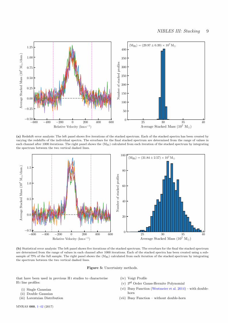
(a) Redshift error analysis: The left panel shows five iterations of the stacked spectrum. Each of the stacked spectra has been created by

varying the redshifts of the individual spectra. The errorbars for the final stacked spectrum are determined from the range of values in

each channel after 1000 iterations. The right panel shows the 〈MHi 〉 calculated from each iteration of the stacked spectrum by integratingthe spectrum between the two vertical dashed lines.

−600 −400 −200 0 200 400 600

Relative Velocity (km s−1)

−0.5

0.0

0.5

1.0

1.5

Ave

rage

Sta

cked

Mas

s(1

07

M/c

han.)

25 30 35 40

Average Stacked Mass (107 M)

0

20

40

60

80

100

Nu

mb

erof

stac

ked

pro

file

s

〈MHi〉 = (31.84± 2.57)× 107 M

(b) Statistical error analysis: The left panel shows five iterations of the stacked spectrum. The errorbars for the final the stacked spectrum

are determined from the range of values in each channel after 1000 iterations. Each of the stacked spectra has been created using a sub-sample of 75% of the full sample. The right panel shows the 〈MHi 〉 calculated from each iteration of the stacked spectrum by integrating

the spectrum between the two vertical dashed lines.

Figure 5: Uncertainty methods.

that have been used in previous H i studies to characteriseH i line profiles:

(i) Single Gaussian(ii) Double Gaussian(iii) Lorentzian Distribution

(iv) Voigt Profile

(v) 3rd Order Gauss-Hermite Polynomial

(vi) Busy Function (Westmeier et al. 2014) – with double-horn

(vii) Busy Function – without double-horn

MNRAS 000, 1–42 (2017)

10 J. Healy et al.

Fig. A5 shows the 7 functions fitted to the stack of the1000 simulated profiles. Also shown is a table containingthe integrated flux density, a measure of the goodness of fit,and the full-with at half-maximum (FWHM) of the fittedfunction. The user may select any number of the functions,and HISS checks that the user is satisfied with the selectionbefore continuing. A version of Fig. A5 is saved in PNG10

format in the output location as Diagnostic Plot 3. The di-agnostic plot is saved to file if HISS is run in suppress mode(an option the user may select when initialising HISS whichsuppresses all displayed output) so that the user may inspectthe function fit before continuing with the analysis.

2.4.4 Uncertainty calculation

The Uncertainty Module allows for two types of uncertaintycalculations: a statistical error analysis and a redshifterror analysis. The user specifies the type of uncertaintycalculation (the two methods cannot be run simultane-ously). The Uncertainty Module facilitates the storing ofthe final analysis options chosen by the user and uses thoseoptions to repeat the stacking process 1000 times, eachtime with slightly different parameters. Fig. 1 indicates theUncertainty Module as a wrapper around the Stack andAnalysis modules.

1. Redshift error analysis: if the user chooses to engagethe redshift uncertainty calculations, another loop is acti-vated around the Stack and Analysis Modules which repeatsthe two processes one thousand times. In every iteration,the redshift associated with each spectrum in the inputcatalogue is changed by an amount that is selected from anormal distribution with a standard deviation equivalentto the particular spectrum’s redshift uncertainty. Thus, theredshift for each spectrum becomes z = z + dz, where dzhas been sampled from a normal distribution defined byN(µ = z;σ = u(z)).

The result of repeating the stack and analysis processmeans that there are 1000 slightly different versions of thestacked spectrum and their corresponding integrated fluxvalues. Each of the 1000 versions of the analysis object(which each contain a selection of integrated fluxes andthe stacked spectrum data) are stored by the UncertaintyClass. Upon completion, the Uncertainty Class processesthe stored data: the error bars on the spectrum data arecalculated from the minimum and maximum values perchannel of the 1000 stored spectra, the data points aregiven by the mean values. The error-bars on the integratedfluxes are determined from the difference between the meanvalue (which serves as the quoted value) and the 25th and75th percentile.

An example of the stacked spectrum using this errorcalculation method and an average dz = 60 km s−1 is shownin Fig. 5a.

2. Statistical error analysis: the statistical error analy-sis implemented by this module is the Delete-A-Group Jack-

10 Portable Network Graphics

knife (Kott 2001) error method. In the same way as men-tioned above, another loop is activated around the Stack andAnalysis Modules repeating the process a thousand times,however each iteration discards a percentage (as chosen bythe user) of the total catalogue without replacement. The1000 analysed stacked spectra are stored by the UncertaintyModule. The flux values for the final stacked spectrum aretaken as the mean value of the 1000 versions in each chan-nel. The error bars on the flux in each channel are calculatedaccording to

σ(s) =

√√√R − 1

R

R∑n=0(sn − s)2, (8)

where R is the number of repeated estimates (which wouldbe 4 if only 75% of the population was used for eachiteration), sn is the flux for the particular channel of thenth subset, and s is the mean flux value for the particularchannel (Kott 2001; Brown et al. 2015). This is illustratedin Fig. 5b.

The shape of the redshift error analysis profile issmeared out into a more Gaussian shape than the statisticalerror analysis stacked profile due to each spectrum beingallocated its correct redshift plus an offset value. Thisresults in the individual line centres being smeared aroundthe zero point. This was also observed by Maddox et al.(2013).

The choice of preferred error analysis method is left tothe user to decide based on their particular sample selectionand optical catalogue redshift precision.

2.5 Save Results

There are nine possible files that can be saved to the outputlocation – 5 data files and 4 possible diagnostic plots (theseinform user interactions at point 2):

(i) Stacked Catalogue: this text file contains a list of allthe spectra included in the stack. Along with the dataprovided by the user from the input catalogue, thistable also contains the integrated flux density for eachspectrum.

(ii) Output Data: a FITS table file containing the spec-trum data (stacked spectrum, spectral axis and ref-erence spectrum), the fitted parameters of any fittedfunctions, the stacked noise, and if the spectrum hasbeen smoothed then the original version of the spec-trum data is also saved.

(iii) Stacked Spectrum Plot: a PDF file of the stackedspectrum plotted with the fitted functions and thereference spectrum (a version of this is shown in thetop left panel of Fig. A7).

(iv) Stacked Noise Plot: a PDF file of the stacked noise

which has the expected σ/√

N line over-plotted (topright panel of Fig. A7).

(v) Integrated Flux Data File: a table of the calculatedintegrated flux from the different functions as wellas the flux integrated within the galaxy window.This file is saved in Encapsulated Comma SeparatedValue (ecsv) format using the AstroPy ASCII mod-

MNRAS 000, 1–42 (2017)

NIBLES III: Stacking 11

ule, which allows the units of the flux to be saved tofile. Other columns in this file include the goodnessof fit values from the function fits. A version of thistable is shown in the bottom panel of Fig. A7.

(vi) Diagnostic Plot 1: this is the first plot of the stackedspectrum that is displayed and saved upon initialisa-tion of the Analysis Module. (Fig. A4)

(vii) Diagnostic Plot 2: a PNG file that is only producedif the user decides to rebin or smooth the spectrum.This plot is almost identical to Fig. A4.

(viii) Diagnostic Plot 3: a PNG file that is created when theuser selects a function to fit to the stacked spectrum(Fig. A5).

(ix) Diagnostic Plot 4: this plot is only produced if theuncertainties have been calculated. The plot containsa series of histograms showing the spread of the in-tegrated fluxes. Diagnostic Plot 4 is saved to file inPNG format (Fig. A6).

2.6 Displaying the results

Upon conclusion of the analysis of the stacked spectrum, allcalculated quantities and plots are saved to the user-chosenoutput location. Amongst the saved files is a plot of thestacked spectrum which makes this final module an optionalone. The Display module reads in the files saved to disk atthe end of the analysis. The results are then displayed in aneasy to read manner – the stacked spectrum (along with thereference spectrum) is shown on the top left, to the rightof the stacked spectrum is the stacked noise as a functionthe number of profiles. Below the two plots are the statisticsassociated with stacked spectrum, and a table containingthe calculated integrated fluxes. A screenshot of the displaywindow is shown in Fig. A7.

3 APPLICATION OF HISS TO THE NIBLESSURVEY

In this second half of the paper, we will demonstrate someof the capabilities of HISS by stacking different sub-samplesof galaxies observed as part of the Nancay InterstellarBaryon Legacy Extragalactic Survey (NIBLES; van Drielet al. 2016), and re-visiting the well-known H i scalingrelations (e.g. Catinella et al. 2010, 2012, 2013; Brown et al.2015).

NIBLES is a targeted H i survey of galaxies selectedby Mz, a proxy for stellar mass, from the Sloan Digital SkySurvey (SDSS; York et al. 2000). The H i data were obtainedusing the 100 m Nancay Radio Telescope (NRT) in the centreof France. NIBLES provides a unique opportunity to studythe baryonic content in galaxies with a wide range of stellarmass (106 < M?(M) < 1012).

3.1 H i Data

The NIBLES sample of 2600 galaxies was selected fromSDSS Data Release 5 (DR5; Adelman-McCarthy et al.2007). The selected galaxies were chosen to uniformly sam-ple the stellar mass range of the ensemble of galaxies in the

local Universe. The particular selection criteria (van Drielet al. 2016) were as follows:

(i) The target must have both SDSS DR5 spectroscopyand photometry.

(ii) NIBLES targets were limited to the Local Volume:900 < cz < 12000 km s−1.

(iii) In order to study the H i in galaxies as a func-tion of stellar mass, ∼ 150 galaxies were selectedper 0.5 mag bin for −16.5 mag ≤ Mz ≤ −24 mag(H0 = 70 km s−1 Mpc−1), if available. Mz was used asa proxy for stellar mass11;

(iv) In order to maintain a morphologically diverse sam-ple, no colour selection was made.

In addition to these criteria, van Driel et al. (2016), whenselecting the target galaxies tried to avoid objects in andaround the Virgo cluster as well as the ALFALFA α.40footprint (Haynes et al. 2011). The dense environment inthe Virgo cluster is known to have noticeable effects on theH i properties of the galaxies in the region. The distances togalaxies in the Virgo region also have large uncertainties.

The Nancay Radio Telescope (see van Driel et al.for further details) is a 100 m single dish radio telescopelocated in France. The telescope is a transit instrumentwith a collecting area of 6900 m2 and consists of two largereflectors. At 21 cm, the NRT beam spans 3.6′ in rightascension and varies in declination from 22′ − 33′ dependingon the declination of the source; the exact declination sizeof the beam can be determined using Eq. B1.

The spectra were collected from January 2007 to De-cember 2010, for a total of 3500 hours of telescope time.Each target was initially observed for roughly 40 minutesusing successive 40 s ON source and 40 s OFF source point-ings, which was repeated as required and as observing timepermitted. The OFF source pointing was chosen to be 20′Eof each target. The data reduction process is discussed in de-tail by van Driel et al. (2016). Each published spectrum hasa velocity resolution of 18 km s−1 and a typical noise level of2.5 mJy.

3.1.1 Higher-sensitivity Arecibo follow-up H i observations

An indication that stacking Nancay H i spectra may leadto the detection of a significant signal can be found in thehigher sensitivity follow-up observations that were obtainedwith the 305m Arecibo radio telescope, which resulted in ahigh detection rate of NRT non-detections (Butcher et al.2016). Of the Nancay targets, 71 non-detections and 19marginal detections were observed at Arecibo with a fourtimes higher sensitivity (mean rms 0.57 mJy). This led to thedetection of 85% and 89% of the NRT non-detections andmarginal detections, respectively. It should be noted thatmost (59, or 66%) of the re-observed NRT non-detections areblue, low mass galaxies (∼ 106.5 < M? (M) < 108.5) whichare expected to be relatively gas-rich (see § 4). Within the

11 SDSS stellar mass catalogues were not yet publicly availableat the time of the original NIBLES sample selection which was

based on DR5 photometry.

MNRAS 000, 1–42 (2017)

12 J. Healy et al.

same stellar mass range, the 〈FH i〉 of the new Arecibo detec-tions is on average three times lower than for the Nancay de-tections. Alternatively, using the HISS approach to reach thefour times lower Arecibo rms level we could also have stacked16 NRT spectra. The analysis of similar Arecibo data of amuch larger sample of NIBLES Nancay non-detections ofall colours has recently been published by Butcher et al.(2018). The Arecibo data mentioned above were not usedfor the stacking study presented here.

3.1.2 Comparison between NIBLES and other H i surveys

Upon comparison with other single-dish H i surveys (e.g.ALFALFA, HIPASS (Barnes et al. 2001); see Table A.4in van Driel et al. 2016), the ALFALFA α.40 fluxes werefound to be higher than the NIBLES fluxes by a fac-tor α.40/NRT = 1.45 ± 0.17. The comparisons between NRTfluxes and the ALFALFA fluxes, as well as possible reasonsfor the difference in flux scales are discussed in detail in § 4.6in van Driel et al. (2016). In this work, the NIBLES fluxesare quoted. In the event of comparison between NIBLESmeasurements and ALFALFA measurements, the ALFALFAmeasurements are scaled to the NIBLES flux values usingthe ALFALFA/NRT flux ratio mentioned above.

3.2 Optical Data

The optical photometric data used in this work is obtainedfrom the SDSS Data Release 12 where the photometricquality flag was marked clean with no deblended “child”objects. In the DR12 database, the spectroscopic sources(from which the NIBLES sample is derived) are matched tothe “value-added” JHU/MPA catalogues (Brinchmann et al.2004) which contain the stellar masses used in this work.The catalogue provides a number of different measures ofthe stellar mass, however for the purposes of the NIBLESanalyses, the median values are used (Butcher et al. 2018;van Driel et al. 2016).

3.3 NIBLES Stacking Sample

3.3.1 Accounting for known contamination sources

Studies have shown that galaxies which are nearby to thetarget galaxies in terms of both distance on the sky and sys-temic velocity can significantly contribute to the total emis-sion in a target H i galaxy spectrum (Jones et al. 2016; Elsonet al. 2016). For example, Elson et al. (2016) showed thatfor a stacking experiment using simulated Parkes data at 15′resolution at 0.04 < z < 0.13, the average contaminant H imass per galaxy spectrum was ∼ 1.4 × 1010 M. Thus, beforefinalising the sample of spectra for stacking, it is necessaryto remove spectra that are known to have nearby galaxiesthat could contribute significant contaminating emission tothe spectrum. In other works (e.g., Fabello et al. 2012), asecondary source (irrespective of morphology) is consideredto contaminate the target spectrum if it lies spatially withinthe half-power beam width and ±300 km s−1 of the target.In this work, galaxies near the target source are consideredas possible contaminators if

• the secondary galaxy is located spatially within 1.2×

N-S half-power beam width and 2× E-W half-powerbeam width, and• the redshift of the secondary galaxy is within±300 km s−1 of the target redshift.

The above criteria were used to search for sources in boththe SDSS Spectroscopic Database and the NASA/IPAC Ex-tragalactic Database (NED). A total of 761 spectra wereclassified as potentially contaminated using these criteria.For more details see Appendix B.

3.3.2 Defining H i detections vs. non-detections

NIBLES galaxies were originally classified as ‘detected’,‘marginal’ or ‘not detected’ as explained in van Drielet al. (2016) by three independent adjudicators, who usedstatistical parameters describing the profile S/N and alsoinspected all spectra by eye. For this work we wanted abinary classification of ‘detected’ or ‘not detected’ for ourstacking experiments and we wanted to use a method whichdid not rely on human intervention. Various methods existfor finding signals and classifying detections in H i spectra(see for example Saintonge 2007; Verheijen et al. 2007;Haynes et al. 2011; Ramatsoku et al. 2016). Using theoriginal classifications in van Driel et al. (2016) as a guide,we used classification criteria, adapted from Ramatsokuet al. (2016) to reproduce the sample selection of van Drielet al. (2016), while at the same time self-consistently andobjectively classifying the marginal detections as eitherdetections or non-detections. This method produced verysimilar detection classifications to van Driel et al. (2016)with over 96% overlap in the classifications between thetwo schemes for both detections and non-detections, andresulted in the NIBLES marginal detections (52) beingallocated as detections vs. non-detections in a ratio ofone-third to two-thirds in our sample.

Following Ramatsoku et al. (2016) we classify galaxiesas detected if there are a number of consecutive channelsabove a threshold value. The threshold values are set basedon the noise level of the individual spectra which we estimateusing the sub-interquartile range (IQR – half the differencebetween the 75th and 25th flux percentiles). The IQR is lesssensitive to outliers in a distribution than the standard de-viation and therefore eliminates the need for manual mask-ing of the target source and/or artefacts in the spectrumwhen estimating the noise (see Fig. C1). For classificationof NIBLES spectra, we considered a window of 600 km s−1

centred on the target redshift. If any emission, satisfying thecriteria below, was found in the window, the spectrum wasclassified as a detection:

• 1 or more channels with flux density above 5× IQR(within a 400 km s−1 window)• 2 or more consecutive channels above 4× IQR• 4 or more consecutive channels above 3× IQR• 5 or more consecutive channels above 2× IQR.

Visually inspecting the spectra after classificationshowed that some sources had an H i detection in the off-source pointing which presents in the NIBLES spectra as anabsorption-like feature, while other spectra had clear emis-sion features from sources not previously identified in our

MNRAS 000, 1–42 (2017)

NIBLES III: Stacking 13

−24 −22 −20 −18 −16

Mr (mag)

0

1

2

3

4

5

u−r

(mag

)

Baldry et al. (2004)

NIBLES Targets

Figure 6: Optical colour-magnitude diagram for theNIBLES stacking sample galaxies: u−r colours derived fromSDSS model magnitudes corrected for Galactic extinctionas a function of absolute r-band magnitude. The H i non-detected galaxies are plotted in either red or blue basedon their position above or below the Baldry et al. (2004)red/blue colour divider which is indicated by the black line.The grey data points represent the H i detected galaxies.

possible contaminant source search (see § 3.3.1.) Examplesof spectra with these features are presented in Fig. C2. Thesefeatures can bias the stacked spectrum and therefore in or-der to flag these spectra and eliminate them from our sam-ple, we ran the classification algorithm a second time overa wider velocity range (±600 km s−1 centred on the targetredshift and indicated by the vertical green dashed lines inFig. C2), to identify possible positive and negative emissionnot related to the target galaxy. We rejected galaxy spec-tra that had either negative emission satisfying our clas-sification criteria in any part of the larger search window(cz ± 600 km s−1) or positive emission satisfying the criteriaand falling outside a central range of cz ± 200 km s−1 butwithin cz ± 600 km s−1. In total 24 spectra were removedfrom the stacking sample in this way.

3.3.3 Final stacking sample

We excluded from our sample galaxies with M? < 108 Mdue to unreliable SDSS photometry and therefore unreliablestellar masses. Our final catalogue consists of 1000 H i spec-tra deemed free of nearby contaminant emission. Of the 1000sources, 323 were classified as non-detections and 677 as de-tections (see Fig. C3 for examples). The catalogue for thenon-detections can be found in Appendix E.

4 GAS SCALING RELATIONS IN NIBLES

As has been previously stated, the NIBLES sample ismorphologically diverse, and it ranges from gas-rich late-type galaxies to gas-poor early-type galaxies. In order toexplore the contributions from the different morphologicaltypes to the stacked profiles, we separate the stacking

sample into red and blue sub-samples using the Baldryet al. (2004, Eq. 9) optimal colour divider as shown in Fig. 6.

Having separated the full sample into blue and red sub-samples, there are 549 blue galaxies (436 detections, and113 non-detections) and 451 red galaxies (241 detections,and 210 non-detections). The stellar mass distributions forthe full sample and non-detections alone, and each brokendown by colour, are shown in Fig. 7.

It is clear in both the full sample and the non-detectedsample that the blue galaxies are predominantly in the low-M? regime, while the red sample contains mainly high-M?

galaxies. The transition from predominantly blue galaxies topredominantly red galaxies occurs in our full sample aroundM? = 109.5 M which also corresponds to the so-called “gas-richness” threshold (Kannappan et al. 2013) which signifiesthe transition from H i gas-rich galaxies (at lower M?) toH i gas-poor galaxies (at higher M?).

4.1 The average H i properties

We separated the full sample into three samples: all spectra(full sample), detections only, and non-detections only.The spectra are stacked in units of MHi and the resultingspectra are shown in the left column of Fig. 8. The toprow of Fig. 8 shows the stacked profiles for the full sample,detections, and non-detections on the same set of axes;the bottom row shows only the stacked profiles for thenon-detections, enlarged for clarity. The top left panelshows the comparison between the stacked spectra for thefull sample (blue triangles), and the spectra for the sampleof only detections (purple squares) and only non-detections(black filled circles).

The middle and right panels of Fig. 8 show the stackedspectra for the blue and red sub-samples respectively.As indicated by the vertical yellow bands, we integrateover a narrower velocity range for the blue sub-samplescompared to the red sub-samples. The blue stacked spectraare expected to be narrower since the average stellar massof the blue sample is lower than the red sample.

The average H i mass and MHi to M? ratio ( fHi)measured from the stacked profiles for each of the ninesub-samples (all galaxies, all blue galaxies, all red galaxies;all H i detections, blue H i detections, red H i detections;all non-detections, blue non-detections, and red non-detections) are shown in Table D1.

H i stacking is a powerful tool to probe the average H iproperties of various galaxy samples, however one shouldhave a clear idea of the morphological properties of thegalaxies that make up the sample. We have shown howthe stacked H i profiles can change by only looking at blueor red galaxies – we find that the stacked profiles for thered samples are wider than the stacked profiles for theblue samples. This is to be expected based on the bimodaldistribution of local galaxies where the red galaxies onaverage have higher stellar masses, and in line with theTully-Fisher relation, higher rotation velocities (see also

MNRAS 000, 1–42 (2017)

14 J. Healy et al.

8.0 8.5 9.0 9.5 10.0 10.5 11.0 11.5 12.00

25

50

75

100

125

150

175

Nu

mb

erof

gala

xie

s

Full Sample

log M? (M)

8.0 8.5 9.0 9.5 10.0 10.5 11.0 11.5 12.0

Non-detections

Figure 7: The stellar mass distribution for the full sample (left) and the non-detections (right). The grey bars indicate thetotal number of galaxies per bin, while the blue and red lines indicate the number of blue and red galaxies per mass bin. Eachbin is 0.5 dex wide. The dashed green line highlights the “gas-richness” threshold (Kannappan et al. 2013), where gas-richgalaxies are to the left of the line (lower M?) and gas-poor galaxies are to the right of the line (higher M?).

Fabello et al. 2011; Meyer et al. 2016).

We divided our sample into two bins of low and highstellar mass (M? < 109.5 M and M? > 109.5 M) to explorethe average H i properties of blue and red galaxies inthese 2 samples. As outlined earlier in this paper, HISS iscapable of directly determining the average H i mass or H igas fraction from stacked spectra. The H i-to-stellar massfraction (gas fraction or fHi) is a useful tool to probe howgas rich a galaxy or sample of galaxies is. Our results aresummarized in Fig. 9 and the stacked profiles are shown inAppendix D2, with the measured quantities presented inTable D2 and Table D3. Note that all the stacked profileshave S/NALFALFA > 6.5 and are also classified as detectionsaccording to the criteria in § 3.3.2.

These results are consistent with work by Kannappan(2004) which shows that while low mass galaxies tend tohave lower H i masses than their high mass counterparts,the low stellar mass galaxies tend to have higher H i gas frac-tions. The right panel of Fig. 9 highlights what was foundby Brown et al. (2015) that the steep slope of the average〈 fHi〉 vs M? trend (indicated by the black squares and filledcircles) from low to high stellar mass is driven by the pre-dominance of high gas fraction blue galaxies at low stellarmass and the low gas fraction red galaxies at high stellarmass. This trend is seen for both the full stacked sampleand when stacking non-detections alone.

4.2 Gas fractions in NIBLES galaxies

Gas scaling relations have been used in conjunction withstacking (e.g., Fabello et al. 2011, hereafter F11; Brown

et al. 2015, hereafter B15) to study various galaxy proper-ties (star formation, stellar mass, etc.) and their influenceon the H i content of the galaxies. In Fig. 10 we compareNIBLES gas fractions calculated using HISS to gas fractionsfrom Catinella et al. (2013, hereafter C13), F11 and B15.Adopting the method used by B15, we separated the fullNIBLES sample (detections plus non-detections) into binsof log M? with widths of 1 dex. The sample stellar massdistribution is presented in Fig. 7. For the NIBLES samplein Fig. 10 (indicated by the round blue circles), the M?

values represent the mean value in each bin. The NIBLESstacked profiles are presented in Fig. D5 and the measuredquantities are listed in Table 1.

The C13 sample was selected from the GALEX AreciboSDSS Survey (GASS, Catinella et al. 2010, 2013), a surveywith the Arecibo telescope which targeted ∼ 1000 massivegalaxies randomly selected from the overlap between theSDSS DR6 spectroscopic survey and GALEX MediumImaging Survey. The F11 and B15 samples are selectedfrom the overlap between ALFALFA, SDSS and GALEX.The C13 results show weighted average values (the H inon-detections are set to upper limits) while the F11 andB15 results are obtained from H i stacking. To take into ac-count the known flux offset between ALFALFA H i spectraand NIBLES (see § 3.1.2), the B15 and F11 gas fractionshave been scaled by the mean α.40/NRT flux ratio (1.45).The solid green line is the fit from F11 to their gas scalingrelation and the dotted green line represents a linearextrapolation of this trend to lower stellar mass.

Due to the NIBLES sample selection, we are able togo down an order of magnitude lower in stellar mass than

MNRAS 000, 1–42 (2017)

NIBLES III: Stacking 15

0

3

6

9

12

15

Ave

rage

Sta

cked

Mas

s(×

107

M/c

han.)

Nall = 1000

Ndet = 677

Full Sample

Nall = 549

Ndet = 436

Blue Sample

Nall = 451

Ndet = 241

Red Sample All

Det

Non-Det

−500 0 500−2

−1

0

1

2

3

4N = 323

signif. => 8.2σ

−500 0 500

Relative Velocity (km · s−1)

N = 113

signif. => 8.2σ

−500 0 500

N = 210

signif. => 8.2σRef Spec

Non-Det

Uncert

Figure 8: The three columns in the figure above show the stacked profiles for the full sample, blue sample, and red samplerespectively. In the top row are the stacked profiles for all spectra (blue triangles), only detections (purple squares), and onlynon-detections (black circles). The bottom row shows the stacked profiles for the non-detections, the reference spectrum isshown in green, and the grey band represents the uncertainty of the stacked spectrum. The vertical yellow regions in each ofthe panels indicate the region over which the spectra are integrated to obtain the average H i mass, 〈MHi〉.

previous results by B15. For M? > 109 M the NIBLES gasfractions agree well with the results by C13 and the adjustedgas fractions from B15 and F11. Below M? < 109 M, theNIBLES 〈 fHi〉 is lower than the trend set by the higherstellar mass galaxies.

Huang et al. (2012) and Maddox et al. (2015) have pre-viously noted the change in slope of the MHi vs M? relationbetween 108 < M? < 109 M in the H i-selected populationof ALFALFA galaxies where the relation is steeper at lowermass and flatter towards the high mass end. A change inslope is also seen in the ALFALFA fHi-M? scaling relationby Huang et al. (2012) around a similar M? where the slopeis flatter at lower M? and drops more steeply at higher M?.Huang et al. (2012) note that their average gas fractionrelation has an overall offset to higher values as expectedcompared to the optically selected samples by Catinellaet al. (2010) and Cortese et al. (2011) due to the ALFALFAsample bias towards more gas rich galaxies per stellar massbin. Across the mass range investigated, per bin in stellarmass, they also observe a sharp cut-off in number density at

the higher end of the gas fraction distribution, but a largedispersion towards lower gas fractions and note that forsurveys with longer integration times, a lower average fHi

per stellar mass bin would be observed. A similar change inslope towards lower M? would also therefore be expectedfor stellar mass selected samples as for the ALFALFAsample. The divergence of the lowest stellar mass NIBLESgas fraction data point from the higher stellar mass trendsfrom the extrapolated F11 fit is therefore consistent withexpectations based on the H i-selected ALFALFA sampleHuang et al. (2012) gas fraction vs M? relation.

5 SUMMARY

This work has detailed the development of a new 21 cm H ispectral stacking package in Python (H i Stacking Software:HISS); while we have exclusively used H i emission spectrato test HISS, it is capable of stacking emission or absorptionspectra of any characteristic line. HISS takes the spectra for

MNRAS 000, 1–42 (2017)

16 J. Healy et al.

8.5 9.0 9.5 10.0 10.5 11.0

log 〈M?/M〉106

107

108

109

1010

〈MH

i/M〉

NIBLES full catalogue

NIBLES non-detections

8.5 9.0 9.5 10.0 10.5 11.0

log 〈M?/M〉10−3

10−2

10−1

100

101

〈f Hi〉

NIBLES full catalogue

NIBLES non-detections

Figure 9: Average MHi 〈MHi〉 (left), and the 〈MHi/M?〉 mass ratio, the average gas fraction 〈 fHi〉 (right), as a function of M?

for the full NIBLES sample as well as the sub-sample of H i undetected galaxies. Each sample has been split into two stellarmass bins: 108 < M? (M) < 109.5 and 109.5 < M? (M) < 1012. Shown here are the mean M? of the galaxies in each of the twostellar mass bins, for each of the various samples. The round data points represent the non-detections, and the square pointsrepresent the full sample. The blue, red and black data points represent respectively the blue, red and total sub-samples. Theerror bars represent the statistical uncertainties, including on the stacks of non-detections. The stacked profiles which eachdata point represents, are presented in Appendix D2.

log〈M?/M〉 〈 fHi〉 N Significance S/NALFALFA

8.56 1.709 ± 0.089 347 (109) > 8.2σ 174.7

9.60 0.473 ± 0.024 335 (96) > 8.2σ 231.8

10.53 0.093 ± 0.005 272 (93) > 8.2σ 216.6

11.17 0.032 ± 0.005 46 (25) > 8.2σ 49.3

Table 1: Average H i gas fractions 〈 fHi〉 for the scaling relation in Figure 10. The average MHi/M? ratio 〈 fHi〉 values for eachdata point are given along with the statistical uncertainties. The total number of galaxies per bin are given in the columntitled N, with the number of non-detections per bin indicated by the number in brackets. The second-last column gives theGaussian significance of the stacked profile obtained from HISS (see § 2.4.1 for details). The final column gives the S/N of thestacked spectrum calculated by HISS using Eq. 7.

a sample of galaxies along with the accompanying redshiftsrecorded in the galaxy catalogue to produce an averagespectrum from which a number of average properties (e.g.,H i mass 〈MHi〉, H i-to-stellar mass ratio 〈 fHi〉) for thesample may be extracted. HISS also offers the user a choiceof two built-in error analysis methods, and the ability tocharacterise the shape of the stacked spectrum throughfitting a variety of functions.

We have applied HISS to stacking of 1000 H i spectrafrom the Nancay Interstellar Baryon Legacy ExtragalacticSurvey (NIBLES), which is a stellar mass-selected (with nocolour-selection) H i survey of SDSS galaxies in the nearbyUniverse. Due to the wide stellar mass range spanned by

the NIBLES dataset (108 < M? (M) < 1012), extendingan order of magnitude lower than Brown et al. (2015), wewere able to extend the previously studied gas fraction vs.stellar mass gas scaling relation (Brown et al. 2015; Fabelloet al. 2011; Catinella et al. 2013) down to lower average stel-lar mass (〈M?〉 = 108.6 M). With our stellar mass selectedsample, we find good agreement with previous results at highstellar mass. At low stellar mass (M? < 109 M) we observea deviation from the extrapolated high mass relation whichindicates a flattening of the slope in the scaling relation atlow stellar mass qualitatively consistent with the trend seenin the H i-blind, gas-rich ALFALFA sample (Huang et al.2012).

MNRAS 000, 1–42 (2017)

NIBLES III: Stacking 17

8 9 10 11

log〈M?/M〉10−3

10−2

10−1

100

101

〈f Hi〉

Fabello et al. (2011)

Brown et al. (2015)

Catinella et al. (2013)

This work

Figure 10: H i gas fraction 〈 fHi〉 as a function of M? for thefull NIBLES stacking sample, including both detections andnon-detections. Also shown, are 〈 fHi〉 values from Brownet al. (2015) who stacked sub-samples of SDSS-selectedgalaxies with H i data from ALFALFA, and Catinella et al.(2013) who calculated weighted averages for sub-samples ofGASS galaxies. The green line is taken from Fabello et al.(2011) who fitted the slope of the gas scaling relation for asub-sample of ALFALFA galaxies; the solid line representsthe stellar mass range of their sample while the dotted part isa linear extrapolation. The errorbars on the NIBLES datapoints are the statistical uncertainties. The plotted valuesare given in Table 1, and the stacked profiles are shown inFig. D5.

ACKNOWLEDGEMENTS

JH acknowledges the bursary provided by South African Ra-dio Astronomy Observatory; SLB, EE, and JH were sup-ported by the South African National Research Foundation.We thank Barbara Catinella and Kelley Hess for their inputand advice on the design of HISS. JH wishes to thank S.Makhathini and L. Lindroos for helpful conversations dur-ing a trip to OSO, supported by MIDPREP. The NancayRadio Astronomy Facility is operated as part of the ParisObservatory, in association with the Centre National de laRecherche Scientifique (CNRS) and partially supported bythe Region Centre in France. This research has made useof the NASA/IPAC Database (NED) which is operated bythe Jet Propulsion Laboratory, California Institute of Tech-nology, under contract with the Nation Aeronautics andSpace Administration, and data from Sloan Digital Sky Sur-vey (SDSS-III). Funding for SDSS-III has been provided bythe Alfred P. Sloan Foundation, the Participating Institu-tions, the National Science Foundation, and the U.S. De-partment of Energy Office of Science. The SDSS-III website is http://www.sdss3.org/. SDSS-III is managed by theAstrophysical Research Consortium for the Participating In-stitutions of the SDSS-III Collaboration.

REFERENCES

Adelman-McCarthy J. K., et al., 2007, The Astrophysical Journal

Supplement Series, 172, 634

Baldry I. K., Glazebrook K., Brinkmann J., Ivezic Z., LuptonR. H., Nichol R. C., Szalay A. S., 2004, The Astrophysical

Journal, 600, 681

Barnes D. G., et al., 2001, Monthly Notices of the Royal Astro-

nomical Society, 322, 486

Bianchi L., GALEX Team 2000, Memorie della Societa Astrono-mia Italiana, Vol. 71, p.1117, 71, 1117

Booth R. S., de Blok W. J. G., Jonas J. L., Fanaroff B., 2009,

ArXiv eprints, p. 2935

Brinchmann J., Charlot S., Heckman T. M., Kauffmann G.,

Tremonti C., White S. D. M., 2004, ArXiv eprints, astro-ph/0

Brown T., Catinella B., Cortese L., Kilborn V., Haynes M. P.,

Giovanelli R., 2015, Monthly Notices of the Royal Astronom-

ical Society, 452, 2479

Brown T., et al., 2017, Monthly Notices of the Royal Astronomical

Society, 466, 1275

Butcher Z., Schneider S., van Driel W., Lehnert M. D., Minchin

R., 2016, Astronomy & Astrophysics, 596, 20

Butcher Z., Schneider S., van Driel W., Lehnert M. D., 2018,Astronomy & Astrophysics, 619, 14

Catinella B., Cortese L., 2015, Monthly Notices of the Royal As-tronomical Society, 446, 3526

Catinella B., et al., 2010, Monthly Notices of the Royal Astro-

nomical Society, 403, 683

Catinella B., et al., 2012, Astronomy & Astrophysics, 544, 30

Catinella B., et al., 2013, Monthly Notices of the Royal Astro-nomical Society, 436, 34

Chengalur J. N., Braun R., Wieringa M., 2001, Astronomy and

Astrophysics, 372, 768

Cortese L., Catinella B., Boissier S., Boselli A., Heinis S., 2011,

Monthly Notices of the Royal Astronomical Society, 415, 1797

Delhaize J., Meyer M. J., Staveley-Smith L., Boyle B. J., 2013,

Monthly Notices of the Royal Astronomical Society, 433, 1398

Elson E. C., Blyth S. L., Baker A. J., 2016, Monthly Notices ofthe Royal Astronomical Society, 460, 4366

Fabello S., Catinella B., Giovanelli R., Kauffmann G., HaynesM. P., Heckman T. M., Schiminovich D., 2011, Monthly No-

tices of the Royal Astronomical Society, 411, 993

Fabello S., Kauffmann G., Catinella B., Li C., Giovanelli R.,Haynes M. P., 2012, Monthly Notices of the Royal Astronom-

ical Society, 427, 2841

Fernandez X., et al., 2016, The Astrophysical Journal Letters,824, 7

Gavazzi G., Pierini D., Boselli A., 1996, Astronomy and Astro-physics, 312, 397

Gereb K., Morganti R., Oosterloo T. A., Guglielmino G., Pran-

doni I., 2013, Astronomy & Astrophysics, 558, 1

Gereb K., Morganti R., Oosterloo T. A., Hoppmann L., Staveley-

Smith L., 2015, Astronomy & Astrophysics, 580, A43

Haynes M. P., et al., 2011, The Astronomical Journal, 142, 170

Hess K., Luber N., Fernandez X., Gim H., Momjian E., vanGorkom J., CHILES 2018, Monthly Notices of the Royal As-tronomical Society

Holwerda B. W., Blyth S.-L., Baker a. J., 2011, Proceedings ofthe International Astronomical Union, 7, 496

Huang S., Haynes M. P., Giovanelli R., Brinchmann J., 2012, The

Astrophysical Journal, 756, 113

Jaffe Y. L., et al., 2016, Monthly Notices of the Royal Astronom-

ical Society, 461, 1202

Johnston S., et al., 2008, Experimental Astronomy, 22, 151

Jones M. G., Haynes M. P., Giovanelli R., Papastergis E., 2016,

Monthly Notices of the Royal Astronomical Society, 455, 1574

Kannappan S. J., 2004, The Astrophysical Journal, 611, L89

Kannappan S. J., et al., 2013, The Astrophysical Journal, 777, 42

MNRAS 000, 1–42 (2017)

18 J. Healy et al.

Kott P. S., 2001, Journal of Official Statistics, 17, 521

Lah P., et al., 2007, Monthly Notices of the Royal Astronomical

Society, 376, 1357Lah P., et al., 2009, Monthly Notices of the Royal Astronomical

Society, 399, 1447

Maddox N., Hess K. M., Blyth S.-L., Jarvis M. J., 2013, MonthlyNotices of the Royal Astronomical Society, 433, 2613

Maddox N., Hess K. M., Obreschkow D., Jarvis M. J., Blyth S. L.,2015, Monthly Notices of the Royal Astronomical Society,

447, 1610

Matthews L. D., van Driel W., 2000, Astronomy and AstrophysicsSupplement Series, 143, 421

McGaugh S. S., de Blok W. J. G., 1997, Astrophysical Journal,

481, 689Meyer S. A., Meyer M., Obreschkow D., Staveley-Smith L., 2016,

Monthly Notices of the Royal Astronomical Society, 455, 3136

Obreschkow D., Rawlings S., Road K., 2009a, Monthly Notices ofthe Royal Astronomical Society, 394, 1857

Obreschkow D., Croton D., De Lucia G., Khochfar S., Rawlings

S., 2009b, The Astrophysical Journal, 698, 1467Obreschkow D., Klockner H.-R., Heywood I., Levrier F., Rawlings

S., 2009c, The Astrophysical Journal, 703, 1890Ramatsoku M., et al., 2016, Monthly Notices of the Royal Astro-

nomical Society, 460, 923

Rhee J., Zwaan M. A., Briggs F. H., Chengalur J. N., Lah P.,Oosterloo T., van der Hulst T., 2013, Monthly Notices of the

Royal Astronomical Society, 435, 2693

Rhee J., Lah P., Chengalur J. N., Briggs F. H., Colless M., 2016,Monthly Notices of the Royal Astronomical Society, 460, 2675

Roberts M. S., Haynes M. P., 1994, Annual Review of Astronomy

and Astrophysics, 32, 115Saintonge A., 2007, The Astronomical Journal, 133, 2087

Serra P., et al., 2015, Monthly Notices of the Royal Astronomical

Society, 448, 1922Stoughton C., et al., 2002, The Astronomical Journal, 123, 485

Tully R. B., Fisher J. R., 1977, Astronomy and Astrophysics, 54,661

Verheijen M., van Gorkom J. H., Szomoru A., Dwarakanath K. S.,

Poggianti B. M., Schiminovich D., 2007, The AstrophysicalJournal, 668, L9

Verheijen M. A., Oosterloo T. A., Van Cappellen W. A., Bakker

L., Ivashina M. V., Van Der Hulst J. M., 2008, in AIPConference Proceedings. pp 265–271, doi:10.1063/1.2973599,

http://arxiv.org/abs/0806.0234

Werner M. W., et al., 2004, The Astrophysical Journal Supple-ment Series, 154, 1

Westmeier T., Jurek R., Obreschkow D., Koribalski B. S.,

Staveley-Smith L., 2014, Monthly Notices of the Royal As-tronomical Society, 438, 1176

Wieringa M. H., de Bruyn A. G., Katgert P., 1992, Astronomyand Astrophysics, 256, 331

York D. G., et al., 2000, The Astronomical Journal, 120, 1579Zwaan M., van Dokkum P., Verheijen M., Briggs F., 2001, Gas

and Galaxy Evolution, 240, 640van Driel W., et al., 2016, Astronomy & Astrophysics, 595, 71

MNRAS 000, 1–42 (2017)

NIBLES III: Stacking 19

APPENDIX A: DETAILS OF HISS

A1 Running HISS

HISS can be downloaded from https://github.com/healytwin1/HISS. Below is a summary of the README file whichdetails the software requirements as well as how to install and run HISS from the command line.

An example of HISS run-time: to stack the 1000 NIBLES spectra with 1000 jackknife iterations on a standard laptopwith 8GB of RAM, took ∼ 4 − 5 hours.

FIRST TIME USERS: It is recommended to use the graphical interface to populate a config file. The graphical interfaceis called by the ”hiss” executable. To use HISS from the command-line, enter the following command:

python pipeline.py [-h] [-f <filepath+filename>] [-d] [-p] [-s] [-c] [-l]

There are a number of different options that can be used to run this package:optional arguments:

-h, --help show this help message and exit.

-d, --display Option to display progress window during the stacking process.

-p, --saveprogress Option to save progress window during the stacking process.

-s, --suppress Use this flag to suppress all output windows.

Note that [suppress] and [progress] cannot be used simultaneously.

-c, --clean Use [clean] for testing purposes and for stacking noiseless spectra as this option will

bypass any noise-related functions and actions.

-l, --latex This option enables to the use of latex formatting in the plots.

A2 HISS Configuration File

MNRAS 000, 1–42 (2017)

20 J. Healy et al.

Below is the configuration file that is used by HISS. This file is filled by the interface shown in Fig. 2.

Config Parameter GUI Parameter/Section Description

CatalogueFilename Catalogue File Path to catalogue file – this should be the full path

CatalogueColumnNumbers Catalogue Information Column numbers for [Object ID, Filename, Redshift, Redshift

Uncertainty, Stellar Mass, Other Data]. “Other Data” refersto data used to bin the sample - if one of the columns is not

needed leave the column entry as an empty string.

z maxRedshift range

Maximum redshift value of sample.

z min Minimum redshift value of sample.

SpectrumFluxUnit

Input Spectra block

Specify flux density units of input spectra. Values to use in

config file: 1-Jy, 2-mJy, 3-uJy, 4-Jy/beam, 5-mJy/beam, 6-µJy/beam

SpectralAxisUnit Values to use in config file: 1-Hz, 2-kHz, 3-MHz, 4-m/s, 5-km/s

VelocityType The choices here are optical/radio. The default is optical, andshould be changed with care. This option will only appear in

the GUI if a velocity spectral type is chosen.

ChannelWidth This should be entered in the same units as the spectral axis.

This parameter is used as a diagnostic to flag spectra which

have vastly different channel widths than the rest of the sam-ple.

SpectrumLocation Spectra location Full path to location of spectra.

FirstRowInSpectrum Input spectra file info First row of data in spectrum file (numbering starts at 1).This option allows for header information in the spectrum file

to be skipped.

RowDelimiter Data delimiter Spectrum file data delimiter - if the delimiter is whitespace,

use ”none”.

SpectrumColumns Spectrum Data Columns (Axis/Flux

Density)

Column numbers for [freq/vel, flux density].

StackFluxUnit Stacked Spectrum Information Choose unit in which to stack. Choices:1-Jy, 2-M, 3-MHi/M?

H0Cosmology

Choice of H0 – default is 70 km · s−1 ·Mpc−1

Om0 Choice of Ωm,0 – default is 0.3

OutputLocation Output location Full path to where results should be saved.

GalaxyWidth Max galaxy velocity width of sample This is the maximum velocity width in the sample. This valueis used to mask the spectrum where emission is expected as

well as uses to define the integration window. The value can

be changed during the analysis process.

StackedSpectrumLength Velocity width of spectrum This defines the length of the spectrum. There is a hard limitthat this value cannot be less than 3 times the maximumgalaxy velocity width. Default is 2000 km s−1.

WeightOption Select Weighting Function 1-w = 1[default], 2-w = 1rms , 3-w = 1

rms2 , 4-w = 1(D2

Lrms)2

NumberCatalogueObjects Stack entire catalogue If ‘y’ is chosen, need to entire the number of catalogue objectsto stack. This will be set to the length of the catalogue if the

chosen number is larger.

UncertaintyYN Calculate Uncertainties This is a [y]es/[n]o option.

UncertaintyMethod Uncertainty method redshift – uses redshift uncertainties to determine uncertaintyof stacked profile. dagjk – Delete-a-group-jackknife, deter-

mines the statistical uncertainty of stacked profile.

BinYN Stack in different bins? This is a [y]es/[n]o option.

BinInfo Information on bins Column name of data to bin, Bin width, Start of Bin range,End of Bin range

MNRAS 000, 1–42 (2017)

NIBLES III: Stacking 21

A3 Plots created by HISS

MNRAS 000, 1–42 (2017)

22J.Healy

etal.

Figure A1: The top left panel shows where the input spectra lie in the observed frame. The middle left panel shows the now aligned spectrum in the velocity and fluxdensity units in which it will be stacked. The bottom left panel shows how the average noise changes with the addition of each new spectrum. The large panel on theright shows the total stacked spectrum, in black, together with the incoming spectrum in blue.

MN

RA

S000

,1–42

(2017)

NIBLES III: Stacking 23

52200 52400 52600

Recessional Velocity (cz km/s)

−25

0

25

Flu

xD

ens.

(µJy)

(a)

52600 52700 52800 52900 53000 53100 53200

Recessional Velocity (cz km/s)

−25

0

25

Flu

xD

ens.

(µJy)

(b)

39800 39900 40000 40100 40200 40300

Recessional Velocity (cz km/s)

−25

0

25

Flu

xD

ens.

(µJy)

(c)

58100 58200 58300 58400 58500 58600

Recessional Velocity (cz km/s)

−25

0

25

Flu

xD

ens.

(µJy)

(d)

40700 40800 40900 41000 41100

Recessional Velocity (cz km/s)

−25

0

25

Flu

xD

ens.

(µJy)

(e)

58000 58100 58200 58300 58400 58500

Recessional Velocity (cz km/s)

−25

0

25

Flu

xD

ens.

(µJy)

(f)

52200 52400 52600 52800

Recessional Velocity (cz km/s)

−25

0

25

Flu

xD

ens.

(µJy)

(g)

52600 52800 53000 53200

Recessional Velocity (cz km/s)

−25

0

25

Flu

xD

ens.

(µJy)

(h)

40800 40900 41000 41100 41200 41300

Recessional Velocity (cz km/s)

−25

0

25

Flu

xD

ens.

(µJy)

(i)

50100 50150 50200 50250 50300 50350 50400

Recessional Velocity (cz km/s)

−25

0

25

Flu

xD

ens.

(µJy)

(j)

Figure A2: These ten spectra are a selection of the 1000 simulated spectra used in the stacking example throughout thepaper. The spectra are plotted using their native flux density and spectral axes. The simulated, noiseless spectra are shown inorange. Shown in green and purple are the spectra after adding simulated Gaussian noise. The green section of the spectrumshows the part that will be shifted to the centre of the array while the purple section is the part that will be wrapped aroundand appended to the other end of the spectrum in the shifting process. The light blue region shows the section of the profilewhere the galaxy emission is expected to be located. The width of this region is defined by the user and forms part of thegalaxy mask. Panel (j) is an example of a spectrum that will be excluded during the stacking process as there are not enoughchannels outside of the galaxy window.

MNRAS 000, 1–42 (2017)

24 J. Healy et al.

−600 −400 −200 0 200 400 600

Relative Velocity (km/s)

−25

0

25

Flu

xD

ens.

(µJy)

(a)

−2

0

2

4

MH

i (107

M/ch

an.)

−600 −400 −200 0 200 400 600

Relative Velocity (km/s)

−25

0

25

Flu

xD

ens.

(µJy)

(b)

−2

0

2

4

MH

i (107

M/ch

an.)

−600 −400 −200 0 200 400 600

Relative Velocity (km/s)

−25

0

25

Flu

xD

ens.

(µJy)

(c)

−2

0

2

MH

i (107

M/ch

an.)

−600 −400 −200 0 200 400 600

Relative Velocity (km/s)

−25

0

25

Flu

xD

ens.

(µJy)

(d)

−2

0

2

4

MH

i (107

M/ch

an.)

−600 −400 −200 0 200 400 600

Relative Velocity (km/s)

−25

0

25

Flu

xD

ens.

(µJy)

(e)

−2

0

2M

Hi (10

7M/ch

an.)

−600 −400 −200 0 200 400 600

Relative Velocity (km/s)

−25

0

25

Flu

xD

ens.

(µJy)

(f)

−2

0

2

4

MH

i (107

M/ch

an.)

−600 −400 −200 0 200 400 600

Relative Velocity (km/s)

−25

0

25

Flu

xD

ens.

(µJy)

(g)

−2

0

2

4

MH

i (107

M/ch

an.)

−600 −400 −200 0 200 400 600

Relative Velocity (km/s)

−25

0

25

Flu

xD

ens.

(µJy)

(h)

−2

0

2

4

MH

i (107

M/ch

an.)

−600 −400 −200 0 200 400 600

Relative Velocity (km/s)

−25

0

25

Flu

xD

ens.

(µJy)

(i)

−2

0

2

MH

i (107

M/ch

an.)

−600 −400 −200 0 200 400 600

Relative Velocity (km/s)

−25

0

25

Flu

xD

ens.

(µJy)

(j)

−2

0

2

4

MH

i (107

M/ch

an.)

Figure A3: These are the same ten simulated spectra as those plotted in Fig. A2. Shown here in blue are the spectra thathave been converted to their rest frame and centred. The original noise-free versions of each of the spectra are now shownin red. Shown in black are the parts of the extended spectrum that have been filled using the flux from outside the galaxywindow. The right y-axis shows that each of these spectra have also been converted to mass spectra.

MNRAS 000, 1–42 (2017)

NIBLES III: Stacking 25

−600 −400 −200 0 200 400 600

Relative Velocity (km · s−1)

−4

−2

0

2

4

6

8

10

Aver

age

Stac

ked

Mas

s (×

106

M/c

han.)

Stacked Spectrum

Reference Spectrum

Fitted Single Gaussian

Integration Window

1σ noise

Diagnostic Plot 1

Figure A4: Diagnostic Plot 1: this is the first plot of the stacked spectrum displayed to the user. The stacked spectrum isshown in black in the units the user chose as the stacking units. This plot is shown to the user before any spectrum manipulationroutines have been applied to the spectrum. The magenta curve shows the Single Gaussian fit to the spectrum to determinethe significance of the detection. The grey spectrum is the reference spectrum. The green vertical window indicates the partof the spectrum over which the average quantity will be measured. The 1σ noise level is shown by the horizontal blue band.

MNRAS 000, 1–42 (2017)

26J.Healy

etal.

−600 −400 −200 0 200 400 600

Relative Velocity (km/s)

0

2

4

6

8A

vera

geS

tack

edM

ass

(106

M/c

han

)

Single Gaussian

Double Gaussian

Lorentzian Distribution Function

Voigt Profile

3rd Order Gauss-Hermite Polynomial

Busy Function (with double horn)

Busy Function (without double horn)

Average Stacked Spectrum

Fitted Function χ2 χ2red FWHMAverage HI Mass

(M) (km/s)

Single Gaussian 0.62 434.6 2.0 1.56× 108 112.0

Double Gaussian 0.45 228.6 1.1 1.49× 108 121.0

Lorentzian Distribution Function 0.80 1672.4 7.9 1.50× 108 153.0

Voigt Profile 1.10 1054.4 5.0 9.78× 107 87.0

3rd Order Gauss-Hermite Polynomial 0.62 434.2 2.0 1.56× 108 113.0

Busy Function (with double horn) 0.44 224.8 1.1 1.47× 108 122.0

Busy Function (without double horn) 2.00 245.6 1.2 1.46× 108 126.0

Diagnostic Plot 3

RMS Error(× 106 M/chan)

Figure A5: Diagnostic Plot 3: the top panel shows the seven different functions (in various colours) fitted to the stacked spectrum which is represented by the greybars. The table in the bottom panel shows the measured average H i mass as well as three measures of the goodness of fit – here we use the standard χ2 goodness of fitparameter and the χ2

red = χ2/dof, where dof is the number of degrees of freedom, and the last measure is the RMS Error. This plot enables the user to inspect the qualityof the fit to the data before committing to a selection of functions.

MN

RA

S000

,1–42

(2017)

NIB

LESIII:

Stackin

g27

100 105 110Ave. Stacked Mass

(106 M)

0

20

40

60

80

100

120

Nu

mb

erof

stac

ks

Flux Density of Stacked Spectrum

100 105 110Ave. Stacked Mass

(106 M)

0

20

40

60

80

100

120

140

Nu

mb

erof

stac

ks

Single Gaussian

100 105 110Ave. Stacked Mass

(106 M)

0

20

40

60

80

100

Nu

mb

erof

stac

ks

Double Gaussian

115 120 125 130Ave. Stacked Mass

(106 M)

0

20

40

60

80

100

120

140

160

Nu

mb

erof

stac

ks

Lorentzian Distribution Function

50 100Ave. Stacked Mass

(106 M)

0

100

200

300

400

500

600

Nu

mb

erof

stac

ks

Voigt Profile

95 100 105 110Ave. Stacked Mass

(106 M)

0

20

40

60

80

100

120

140

Nu

mb

erof

stac

ks

3rd Order Gauss-Hermite Polynomial

100 120 140 160Ave. Stacked Mass

(106 M)

0

100

200

300

400

500

Nu

mb

erof

stac

ks

Busy Function (with double horn)

100 120 140Ave. Stacked Mass

(106 M)

0

50

100

150

200

250

300

350

400

Nu

mb

erof

stac

ks

Busy Function (without double horn)

-5 0 5

km/s

0

50

100

150

200

250

300

Nu

mb

erof

stac

ks

Mean of Single Gaussian Fit

0.6 0.7 0.8Ave. Stacked Mass

(106 M)

0

20

40

60

80

100

120

Nu

mb

erof

stac

ks

RMS of Stacked Spectrum

Diagnostic Plot 4

Figure A6: Diagnostic Plot 4: each panel shows a histogram of the average stacked mass measured from each profile fit for each of the 1000 stacking iterations (i.e.stacks). This plot provides a picture of how well each function was fit. It is from these histograms that the best estimate of the average quantity and associated error arecalculated.

MN

RA

S000

,1–42

(2017)

28J.Healy

etal.

-600.0 -400.0 -200.0 0.0 200.0 400.0 600.0

Relative Velocity (km/s)

−2

−1

0

1

2

3

4

Ave

rage

Sta

cked

Mas

s(1

06M/c

han

)

Reference Spectrum

Single Gaussian

Stacked Spectrum

100 101 102

Number of stacked spectra

10−5

Sta

cked

Ave

rage

Noi

se(J

y)

Number of galaxy profiles included in Stacked Spectrum: 100 The peak signal-to-noise ratio: 20The significance of the peak: > 8. 2σ (p-value = 1. 45 × 10−139) The ALFALFA signal-to-noise ratio: 70Integrated signal-to-noise ratio: 54

Fitted Function Average HI Mass (M)

Average HI Mass Uncertainty (M)

Fit ChiSquare FWHM (km/s)

Single Gaussian 9.53× 107 2.65× 106 0.14 12 175.0

Average Mass of Stacked Spectrum 9.22× 107 2.60× 106 0 0 175.0

RMS Error(× 106 M/chan)

Figure A7: Screen shot of the output in full display mode. The top left panel shows the final average stacked spectrum with errorbars in black, and the chosen fittedSingle Gaussian overlaid in blue. The top right panel shows the stacked noise as a function of the number of profiles in grey; overlaid in green is the theoretical responseto stacked noise: σ/

√N. The bottom half of the figure contains the table of measured quantities (average H i mass and associated uncertainty), as well as the χ2 and RMS

Error calculated from the function fit to the stacked spectrum. The second entry in the table (Average Mass of Stacked Spectrum) shows the quantities measured directlyfrom the stacked spectrum over the range specified by the user. The S/N statistics, as discussed in § 2.4.1, for the stacked profile are given in the text above the table.

MN

RA

S000

,1–42

(2017)

NIBLES III: Stacking 29

APPENDIX B: ACCOUNTING FOR KNOWN NEARBY CONTAMINATION

The Nancay telescope has a large beam which extends between 22′ − 33′ in the N-S direction depending on the declination ofthe source. The change in the N-S beam width can be approximated by the polynomial

y = (4.02 × 10−9) x5 − (6.90 × 10−8) x4 + (3.63 × 10−6) x2 + (5.45 × 10−3) x + 21.95 (B1)

where y is the beam width in arcminutes and x is the declination in degrees (Matthews & van Driel 2000, Fig. 1.).

In this work, galaxies near the target source are considered as possible contaminators if

• the secondary galaxy is located spatially within 1.2× N-S half-power beam width and 2× E-W half-power beam width,and• the redshift of the secondary galaxy is within ±300 km s−1 of the target redshift.

A number of the target galaxies were found to have possible contaminators with very small angular separation distances.Upon inspection of the optical images for these sources, it was discovered that the possible contaminators were, in fact, partof the target galaxy. The SDSS pipeline has a known issue of de-blending large sources, particularly those with knots of starformation. In order not to over-classify the contaminant sources, a new criterion was therefore introduced to the search: thecontaminant source must lie outside the edge of the target source, as defined as twice the r-band Petrosian radius (rP), whichaccording to Stoughton et al. (2002) is a good estimate of the size of the galaxy. Fig. B1 is an illustration of the method usedto find any secondary contaminating sources.

MNRAS 000, 1–42 (2017)

30J.Healy

etal.

2

3000 3500 4000 4500 5000Vopt (km/s)

10

0

10

20

30

Flu

xD

ensi

ty(m

Jy)

= 12:12:31.1 = 29:10:08.1 (183.130, 29.169)M = 3.650 1010 MNUV r = n/aConfusion Tag: C1

Galaxy Windowcz +/- 300 km/s

NGC 4175 (source 3688)

Gal. Identifier cz Separation Vel. Separationkm / s arcmin km / s

NGC 4175 4112 0 0NGC 4174 4045 1.5 67NGC 4169 3784 2.76 328NGC 4173 1127 3.11 2985KISSBx 37 10433 10.9 6320

1

1

Close-up of the target(3.5’ x 3.5’)

Galaxy in beam and spectrum, but not galaxy window

Target galaxyGalaxy in galaxy window

Galaxies in beam and survey volume, but not spectrum

1.2

x be

am h

eigh

t

8’

2 x r-band Petrosian radius

FWHM of Nancay beam (3.6' x 22'-33' [22.15' at this declination])

Figure B1: Illustration of the method used to find any secondary contaminating sources. On the left of the figure is an SDSS optical image that is 8′ wide and1.2 × beam in declination centred on the coordinates of the target galaxy. Overlaid in red is the half-power size of the beam; the yellow circle has a radius of 2rP whichindicates the estimated size of the galaxy. The magenta open circular marker indicates the target source while the blue, green, and orange open circular markers indicatesecondary targets in the entire survey velocity range (900 < cz < 12000 km s−1). Each of the targets highlighted in the large optical image are listed in the table to theright. The galaxies that are in the survey volume, but whose recessional velocities are not in the spectrum velocity range, are indicated by the orange circles. The greencircles highlight galaxies that are within the velocity range covered by the spectrum – these sources are also marked on the spectrum by the green dashed vertical lines.The blue circled sources are the ones that are considered contamination sources. These sources have a redshift (highlighted by the dashed blue line on the spectrum) thatis within ±300 km s−1 of the target redshift (indicated by the magenta line on the spectrum). The small optical image below the table is a 3.5′ × 3.5′ close-up centred onthe target source.

MN

RA

S000

,1–42

(2017)

NIBLES III: Stacking 31

APPENDIX C: DEFINING A SAMPLE OF H i NON-DETECTIONS

2500 3000 3500 4000 4500 5000 5500

−20

−10

0

10

20

Flu

xD

ensi

ty(m

Jy)

1σ interquartile range2σ interquartile range3σ interquartile range

4σ interquartile range5σ interquartile range

Possible absorption

Possible emission

Edge of 1200km/s widebuffer zone

(cz +/− 600km/s)

UGC 05129 – source: 4220

NIBLES Spectrum

Galaxy Window

Vopt (km/s)Interquartile range

Possible Absorption

Possible Emission

Galaxy window(cz ± 300 km/s)

Figure C1: Graphic example of how the detection algorithm flags different features in a spectrum. The spectrum used in thisexample is classified as a detection. The criteria we used for defining H i detections is outlined in § 3.3.2. Using these criteriawe reproduced with 96 percent overlap, the detection and non-detection classifications published in van Driel et al. (2016).The marginal detections in van Driel et al. (2016) were classified in an approximately one-third/two-thirds ratio as detectionsvs. non-detections respectively.

MNRAS 000, 1–42 (2017)

32 J. Healy et al.

3000 3500 4000 4500 5000

Vopt (km/s)

−5

0

5

10

15

20

Flu

xD

ensi

ty(m

Jy)

(a)

SHOC 071 – source: 5348

1250 1500 1750 2000 2250 2500 2750

Vopt (km/s)

−20

−10

0

10

20

30

40

50

Flu

xD

ensi

ty(m

Jy)

(b)

UGC 6307 – source: 5794

2500 3000 3500 4000

Vopt (km/s)

−7.5

−5.0

−2.5

0.0

2.5

5.0

7.5

10.0

12.5

Flu

xD

ensi

ty(m

Jy)

(c)

UGC 09235 – source: 6058

3500 4000 4500 5000

Vopt (km/s)

−30

−20

−10

0

10

20

30

Flu

xD

ensi

ty(m

Jy)

(d)

KUG 0817+228 – source: 5534

Possible Absorption

Possible Emission

NIBLES Spectrum5σnoise

4σnoise

2σnoise

Galaxy Window

Interquartile range

Figure C2: Sources flagged by the second run of the detection algorithm as containing emission/absorption not related tothe target galaxy. All four sources were removed from the sample. Panels (b) and (d) show evidence of an H i detection in theoff-source pointing. Panels (a) and (c) show clear H i detections that are not associated with sources previously identified inour contaminant source search. The vertical red line in each panel indicates the optical redshift of the target source.

MNRAS 000, 1–42 (2017)

NIBLES III: Stacking 33

3500 3750 4000 4250 4500 4750 5000

Vopt (km/s)

−4

−2

0

2

4

Flu

xD

ensi

ty(m

Jy)

(a)

ASK 147870 – source: 3788

1500 2000 2500 3000

Vopt (km/s)

−15

−10

−5

0

5

10

Flu

xD

ensi

ty(m

Jy)

(b)

2MASX J14421771+6052290 – source: 6111

5500 5750 6000 6250 6500 6750 7000

Vopt (km/s)

−5.0

−2.5

0.0

2.5

5.0

7.5

Flu

xD

ensi

ty(m

Jy)

(c)

ASK 139485 – source: 5034

4500 4750 5000 5250 5500 5750 6000

Vopt (km/s)

−10

−5

0

5F

lux

Den

sity

(mJy)

(d)

IC 1226 – source: 4846

1000 1250 1500 1750 2000 2250 2500

Vopt (km/s)

−10

−5

0

5

10

Flu

xD

ensi

ty(m

Jy)

(e)

IC 2450 – source: 2818

750 1000 1250 1500 1750 2000

Vopt (km/s)

−5

0

5

Flu

xD

ensi

ty(m

Jy)

(f)

IC 3096 – source: 2906

Possible Absorption

Possible Emission

NIBLES Spectrum5σnoise

4σnoise

2σnoise

Galaxy Window

Interquartile range

Figure C3: Examples of NIBLES spectra classified as H i detections (left column) and not classified as detections (rightcolumn) – i.e. non-detections. Panel (a) Classified as a detection with ≥ 5 consecutive resolution elements with flux density> 2× IQR. Panel (c) Classified as a detection with ≥ 1 consecutive resolution elements with flux density > 5× IQR. Panel (e)Classified as a detection with 1 resolution element with flux density > 5× IQR. The vertical red line in each panel indicatesthe optical redshift of the target source. Panels (a), (c), (e) are also identified by van Driel et al. (2016) as detections, howeveronly panel (c) would be identified as a detection using the S/N criterion used by ALFALFA.

MNRAS 000, 1–42 (2017)

34 J. Healy et al.

APPENDIX D: STACKING NIBLES GALAXIES

D1 Quantities measured from the stacked spectra

Full Sample Blue Sample Red Sample

1000 549 451 N

> 8.2/> 8.2 > 8.2/> 8.2 > 8.2/> 8.2 σMHi/σfHi

63.1/204.5 289.3/182.8 26.9/112.7 S/NALFALFA,MHi/ S/NALFALFA,fHi

All 1.4939±0.0024 (sys)±0.0572 (stat) × 109 1.4716±0.0028 (sys)

±0.0715 (stat) × 109 1.5155±0.0042 (sys)±0.0946 (stat) × 109 〈MHi〉 (M)

1.795 × 1010 5.641 × 109 3.280 × 1010 〈M?〉 (M)

0.7776±0.0020 (sys)±0.0358 (stat) 1.2100±0.0038 (sys)

±0.0585 (stat) 0.2533±0.0011 (sys)±0.0321 (stat) 〈 fHi〉

677 436 241 N

> 8.2/7 > 8.2/> 8.2 > 8.2/> 8.2 σMHi/σfHi

61.2/339.4 194.9/242.6 25.9/122.3 S/NALFALFA,MHi/ S/NALFALFA,fHi

Detections 2.1231±0.0030 (sys)±0.0825 (stat) × 109 1.5926±0.0026 (sys)

±0.0864 (stat) × 109 2.5806±0.0080 (sys)±0.1728 (stat) × 109 〈MHi〉 (M)

1.519 × 1010 5.837 × 109 3.226 × 1010 〈M?〉 (M)

1.0802±0.0021 (sys)±0.0487 (stat) 1.3222±0.0038 (sys)

±0.0739 (stat) 0.3409±0.0017 (sys)±0.0402 (stat) 〈 fHi〉

323 113 210 N

> 8.2/> 8.2 > 8.2/> 8.2 > 8.2/7.7 σMHi/σfHi

21.1/32.5 18.7/27.6 8.6/8.8 S/NALFALFA,MHi/ S/NALFALFA,fHi

Non-detections 1.5183±0.0409 (sys)±0.3251 (stat) × 108 2.4888±0.0589 (sys)

±0.4674 (stat) × 108 1.1879±0.0577 (sys)±0.4310 (stat) × 108 〈MHi〉 (M)

2.536 × 1010 4.428 × 109 3.351 × 1010 〈M?〉 (M)

0.1408±0.0039 (sys)±0.0277 (stat) 0.3780±0.0098 (sys)

±0.0710 (stat) 0.0349±0.0013 (sys)±0.0078 (stat) 〈 fHi〉

Table D1: Average quantities obtained from stacking the NIBLES galaxies in colour sub-samples and the full sample. Theaverage H i mass values are calculated from the stacked spectra shown in Fig. 8. Gaussian significance values (i.e. σMHi

/σfHi)

of > 8.2σ have corresponding p-values that are too small to be numerically resolved by a computer, thus have been assignedthe significance value of the smallest resolvable p-value.

D2 Stacked Profiles for Fig. 9 and Fig. 10

MNRAS 000, 1–42 (2017)

NIBLES III: Stacking 35

N 〈MHi〉 (M) σMHiS/NALFALFA,MHi

〈 fHi〉 σfHiS/NALFALFA,fHi

Full Catalogue (all) 521 7.46 ± 0.33 × 108 > 8.2 277.7 1.372 ± 0.069 > 8.2 205.7

Full Catalogue (blue) 401 8.00 ± 0.39 × 108 > 8.2 232.8 1.563 ± 0.074 > 8.2 190.5

Full Catalogue (red) 120 5.74 ± 0.63 × 108 > 8.2 196.0 0.740 ± 0.107 > 8.2 127.3

Non-detections (all) 156 12.69 ± 2.47 × 107 > 8.2 35.1 0.299 ± 0.050 > 8.2 33.7

Non-detections (blue) 97 18.25 ± 3.95 × 107 > 8.2 29.5 0.437 ± 0.077 > 8.2 28.1

Non-detections (red) 59 4.09 ± 1.08 × 107 6 11.1 0.095 ± 0.027 5.9 7.5

Table D2: Average quantities and statistical errors obtained from HISS for Fig. 9 for the low stellar mass sample(108 < M? (M) < 109.5). The results with Gaussian significance values of > 8.2 have corresponding p-values that are toosmall to be numerically resolved by a computer, thus have been assigned the significance value of the smallest resolvablep-value.

N 〈MHi〉 (M) σMHiS/NALFALFA,MHi

〈 fHi〉 σfHiS/NALFALFA,fHi

Full Catalogue (all) 479 2.25 ± 0.11 × 109 > 8.2 54.2 0.132 ± 0.007 > 8.2 172.6

Full Catalogue (blue) 148 3.26 ± 0.22 × 109 > 8.2 171.6 0.256 ± 0.014 > 8.2 203.0

Full Catalogue (red) 331 1.87 ± 0.13 × 109 > 8.2 33.3 0.077 ± 0.005 > 8.2 93.9

Non-detections (all) 174 1.89 ± 0.60 × 108 > 8.2 16.6 0.013 ± 0.003 > 8.2 19.0

Non-detections (blue) 17 6.58 ± 1.86 × 108 8 12.1 0.057 ± 0.015 4.6 10.8

Non-detections (red) 157 1.45 ± 0.54 × 108 7.9 8.0 0.010 ± 0.003 > 8.2 16.0

Table D3: Same as Table D2 but for the high stellar mass sample (109.5 < M? (M) < 1012).

MNRAS 000, 1–42 (2017)

36 J. Healy et al.

−500 0 500

Velocity (km/s)

0

2

4

6

8

Ave

rage

Sta

cked

Mas

s(×

10

7M/ch

an)

(a) signif. = > 8.2σ

−500 0 500

Velocity (km/s)

0.00

0.05

0.10

0.15

Ave

rage

Sta

cked

Gas

Fra

ctio

n(M/M?/c

han

)

(b)signif. = > 8.2σ

−500 0 500

Velocity (km/s)

0

2

4

6

8

Ave

rage

Sta

cked

Mass

(×10

7M/ch

an

)

(c) signif. = > 8.2σ

−500 0 500

Velocity (km/s)

0.00

0.05

0.10

0.15

0.20

Ave

rage

Sta

cked

Gas

Fra

ctio

n(M/M?/ch

an)

(d)signif. = > 8.2σ

−500 0 500

Velocity (km/s)

0

2

4

Ave

rage

Sta

cked

Mas

s(×

107

M/c

han

)

(e) signif. = > 8.2σ

−500 0 500

Velocity (km/s)

0.00

0.02

0.04

0.06

0.08

Ave

rage

Sta

cked

Gas

Fra

ctio

n(M/M

?/ch

an)

(f)signif. = > 8.2σ

Figure D1: Stacked profiles for the full sample of H i detections and non-detections with 108 < M?(M) < 109.5. The leftcolumn (panels a, c & e) shows the stacked profiles from which the average H i mass (〈MHi〉) is measured and the right column(panels b, d & f) shows the stacked profiles from which the average gas fraction (〈 fHi〉) is measured. The stacked profiles forall sources in this sample are shown in the top row. The middle row shows the red sub-sample, and the bottom row showsthe blue sub-sample. The shading around each spectrum indicates the uncertainty in each channel calculated based on theredshift errors. The green dot-dashed lines in every panel mark the section of the stacked profiles used to measure the 〈MHi〉and 〈 fHi〉. These spectra correspond to the measurements of 〈MHi〉 and 〈 fHi〉 presented in Fig. 9. The measurements madefrom the above spectra can be found in Table D2.

MNRAS 000, 1–42 (2017)

NIBLES III: Stacking 37

−500 0 500

Velocity (km/s)

0

5

10

15

Ave

rage

Sta

cked

Mass

(×10

7M/ch

an

)

(a) signif. = > 8.2σ

−500 0 500

Velocity (km/s)

0.000

0.002

0.004

0.006

0.008

0.010

Ave

rage

Sta

cked

Gas

Fra

ctio

n(M/M

?/ch

an)

(b)signif. = > 8.2σ

−500 0 500

Velocity (km/s)

0

5

10

15

20

25

Ave

rage

Sta

cked

Mas

s(×

107

M/ch

an)

(c) signif. = > 8.2σ

−500 0 500

Velocity (km/s)

0.000

0.005

0.010

0.015

0.020A

vera

geS

tack

edG

as

Fra

ctio

n(M/M?/ch

an

)

(d)signif. = > 8.2σ

−500 0 500

Velocity (km/s)

0

2

4

6

8

10

Ave

rage

Sta

cked

Mas

s(×

107

M/c

han

)

(e) signif. = > 8.2σ

−500 0 500

Velocity (km/s)

0.000

0.001

0.002

0.003

0.004

Ave

rage

Sta

cked

Gas

Fra

ctio

n(M/M

?/c

han

)

(f)signif. = > 8.2σ

Figure D2: Same as Fig. D1, but for the sample with 109.5 < M?(M) < 1012. The measurements made from the abovespectra can be found in Table D3.

MNRAS 000, 1–42 (2017)

38 J. Healy et al.

−500 0 500

Velocity (km/s)

−0.5

0.0

0.5

1.0

1.5

Ave

rage

Sta

cked

Mas

s(×

107

M/c

han

)

(a) signif. = > 8.2σ

−500 0 500

Velocity (km/s)

−0.02

0.00

0.02

0.04

Ave

rage

Sta

cked

Gas

Fra

ctio

n(M/M?/ch

an)

(b)signif. = > 8.2σ

−500 0 500

Velocity (km/s)

−1

0

1

2

3

Ave

rage

Sta

cked

Mass

(×10

7M/c

han

)

(c) signif. = > 8.2σ

−500 0 500

Velocity (km/s)

−0.02

0.00

0.02

0.04

0.06

0.08

Ave

rage

Sta

cked

Gas

Fra

ctio

n(M/M?/c

han

)

(d)signif. = > 8.2σ

−500 0 500

Velocity (km/s)

−0.2

0.0

0.2

0.4

Ave

rage

Sta

cked

Mas

s(×

10

7M/c

han

)

(e) signif. = 6σ

−500 0 500

Velocity (km/s)

−0.010

−0.005

0.000

0.005

Ave

rage

Sta

cked

Gas

Fra

ctio

n(M/M

?/c

han

)

(f)signif. = 5.9σ

Figure D3: Same as Fig. D1, but for the sample of only H i non-detections with 108 < M?(M) < 109.5. Table D2 containsthe measurements made from the above spectra.

MNRAS 000, 1–42 (2017)

NIBLES III: Stacking 39

−500 0 500

Velocity (km/s)

−2

−1

0

1

2

Ave

rage

Sta

cked

Mas

s(×

107

M/c

han

)

(a) signif. = > 8.2σ

−500 0 500

Velocity (km/s)

−0.0005

0.0000

0.0005

0.0010

Ave

rage

Sta

cked

Gas

Fra

ctio

n(M/M?/c

han

)

(b)signif. = > 8.2σ

−500 0 500

Velocity (km/s)

−5

0

5

10

Ave

rage

Sta

cked

Mass

(×10

7M/c

han

)

(c) signif. = 8σ

−500 0 500

Velocity (km/s)

−0.005

0.000

0.005A

vera

geS

tack

edG

as

Fra

ctio

n(M/M?/c

han

)

(d)signif. = 4.6σ

−500 0 500

Velocity (km/s)

−2

−1

0

1

2

Ave

rage

Sta

cked

Mas

s(×

107

M/c

han

)

(e) signif. = 7.9σ

−500 0 500

Velocity (km/s)

−0.00050

−0.00025

0.00000

0.00025

0.00050

0.00075

Ave

rage

Sta

cked

Gas

Fra

ctio

n(M/M

?/c

han

)

(f)signif. = > 8.2σ

Figure D4: Same as Fig. D1, but for the sample of H i non-detections with 109.5 < M?(M) < 1012. Table D3 contains themeasurements made from the above spectra.

MNRAS 000, 1–42 (2017)

40 J. Healy et al.

−500 0 500

Velocity (km/s)

0.00

0.05

0.10

0.15

0.20

Ave

rage

Sta

cked

Gas

Fra

ctio

n(M/M?/c

han

)

(a) signif. = > 8.2σ

108 < M? (M) < 109

−500 0 500

Velocity (km/s)

0.00

0.01

0.02

0.03

0.04

Ave

rage

Sta

cked

Gas

Fra

ctio

n(M/M?/c

han

)

(b) signif. = > 8.2σ

109 < M? (M) < 1010

−500 0 500

Velocity (km/s)

0.000

0.001

0.002

0.003

0.004

0.005

Ave

rage

Sta

cked

Gas

Fra

ctio

n(M/M?/ch

an

)

(c) signif. = > 8.2σ

1010 < M? (M) < 1011

−500 0 500

Velocity (km/s)

0.0000

0.0005

0.0010

0.0015

Ave

rage

Sta

cked

Gas

Fra

ctio

n(M/M?/ch

an

)

(d) signif. = > 8.2σ

1011 < M? (M) < 1012

Figure D5: All detections and non-detections stacked in bins of stellar mass. The bins increase in stellar mass from panel(a) to (d). The green dot-dashed lines in every panel mark the section of the stacked profiles used to measure the 〈 fHi〉. Thegray band around the spectrum represents the uncertainty of the stacked spectrum. These spectra correspond to the 〈 fHi〉measurements in Fig. 10. See Table 1 for measured quantities.

MNRAS 000, 1–42 (2017)

NIBLES III: Stacking 41

APPENDIX E: CATALOGUE OF H i NON-DETECTIONS

Table E1: Data for the H i non-detections in the stacking sample. The full table is available online.

Source RA Dec Name Vopt u − r Mr M?

[log]

(J2000) km s−1 mag mag M

1926 11 23 18.84 03 57 18.78 CGCG 039-161 1582 ± 19 1.91 −16.18 8.23

1954 11 49 12.79 −03 39 34.64 PGC 1068442 1572 ± 3 1.57 −15.78 8.04

2012 12 19 21.12 04 46 24.49 ASK 173829 2065 ± 2 1.61 −15.87 8.09

2244 14 04 15.84 04 06 43.85 UGC 08986 1239 ± 3 2.19 −17.79 9.08

2272 14 25 08.99 −01 06 48.52 CGCG 019-019 2643 ± 3 2.11 −17.94 9.21

2442 15 17 29.45 03 35 07.94 PGC 3124577 1882 ± 2 1.62 −15.69 8.03

2525 09 35 44.04 31 42 19.68 NGC 2918 6756 ± 2 2.65 −22.64 11.28

2533 10 06 07.44 47 15 45.53 NGC 3111 7437 ± 2 2.68 −22.52 11.19

2535 14 30 25.58 11 55 40.77 NGC 5644 7649 ± 2 2.72 −22.87 11.33

2541 13 53 38.43 36 08 02.57 NGC 5352 7956 ± 3 2.81 −22.64 11.26

2565 00 35 59.83 −10 07 18.07 NGC 0163 5917 ± 4 2.70 −22.05 11.01

2574 11 00 35.40 12 09 41.65 NGC 3491 6351 ± 2 2.72 −21.98 11.06

2589 12 19 32.09 49 48 56.71 UGC 07367 4093 ± 2 2.60 −21.45 10.78

2597 12 19 32.59 56 44 11.69 NGC 4271 4756 ± 2 2.82 −21.84 10.93

2606 14 41 32.96 38 51 04.95 UGC 09473 4669 ± 2 2.17 −21.54 10.80

2614 12 12 17.27 13 12 18.72 NGC 4168 2273 ± 2 2.44 −21.43 10.63

2615 12 32 47.65 63 56 21.18 NGC 4512 2516 ± 1 2.72 −20.75 10.60

2661 10 36 38.44 14 10 15.97 NGC 3300 3017 ± 1 2.54 −21.02 10.53

2675 12 08 09.62 10 22 43.96 NGC 4119 1651 ± 2 2.28 −19.74 10.05

2682 12 27 13.34 12 44 05.22 NGC 4425 1891 ± 1 2.39 −20.42 10.22

2688 12 24 05.01 11 13 05.04 NGC 4352 2083 ± 1 2.36 −20.12 10.08

2710 12 27 02.54 15 27 41.34 NGC 4421 1551 ± 1 2.58 −20.15 10.04

2715 14 05 12.42 55 44 30.67 NGC 5475 1647 ± 1 2.54 −19.58 9.98

2731 12 37 48.38 05 22 06.69 NGC 4580 1035 ± 2 2.37 −19.23 9.75

2742 12 15 59.87 66 13 51.00 NGC 4221 1314 ± 1 2.51 −19.48 9.83

2743 10 12 41.25 03 07 45.79 NGC 3156 1266 ± 29 1.99 −19.14 9.42

2744 11 06 32.10 11 23 07.51 NGC 3524 1357 ± 1 2.36 −19.08 9.71

2756 11 08 40.38 57 13 48.71 NGC 3530 1876 ± 1 2.42 −18.95 9.69

2769 12 25 18.78 64 56 00.52 NGC 4391 1320 ± 1 2.52 −18.73 9.58

2770 13 00 10.57 12 28 59.92 NGC 4880 1362 ± 3 2.24 −19.29 9.51

2775 12 22 04.11 12 47 14.95 NGC 4306 1520 ± 3 2.21 −18.70 9.35

2789 11 21 24.99 03 00 50.23 NGC 3643 1742 ± 2 2.28 −18.67 9.53

2790 12 38 17.87 13 06 35.64 NGC 4584 1715 ± 3 2.01 −18.96 9.46

2795 12 41 59.35 12 56 34.27 NGC 4620 1125 ± 3 2.09 −18.63 9.24

MNRAS 000, 1–42 (2017)

42 J. Healy et al.

↵ = 11h23m18.8s

= 0357018.800

500 1000 1500 2000 2500

Vopt (km/s)

0

5Flu

xD

ens.

(mJy)

CGCG 039-161 (Source 1926)

↵ = 11h49m12.8s

= 339034.600

500 1000 1500 2000

Vopt (km/s)

0

5

Flu

xD

ens.

(mJy)

PGC 1068442 (Source 1954)

↵ = 12h19m21.1s

= 0446024.500

1500 2000 2500 3000

Vopt (km/s)

0

5

Flu

xD

ens.

(mJy)

ASK 173829 (Source 2012)

↵ = 14h04m15.8s

= 0406043.800

500 1000 1500 2000 2500

Vopt (km/s)

0

5

Flu

xD

ens.

(mJy)

UGC 08986 (Source 2244)

↵ = 14h25m09.0s

= 106048.500

2000 2500 3000 3500 4000

Vopt (km/s)

0

5

Flu

xD

ens.

(mJy)

CGCG 019-019 (Source 2272)

↵ = 15h17m29.4s

= 0335007.900

1500 2000 2500 3000

Vopt (km/s)

0

5

Flu

xD

ens.

(mJy)

PGC 3124577 (Source 2442)

↵ = 09h35m44.0s

= 3142019.700

5500 6000 6500 7000 7500 8000

Vopt (km/s)

0

5

Flu

xD

ens.

(mJy)

NGC 2918 (Source 2525)

↵ = 10h06m07.4s

= 4715045.500

6500 7000 7500 8000

Vopt (km/s)

0

5

Flu

xD

ens.

(mJy)

NGC 3111 (Source 2533)

↵ = 14h30m25.6s

= 1155040.800

7000 7500 8000 8500 9000 9500

Vopt (km/s)

0

5

Flu

xD

ens.

(mJy)

NGC 5644 (Source 2535)

↵ = 13h53m38.4s

= 3608002.600

4000 5000 6000 7000 8000

Vopt (km/s)

0

5

Flu

xD

ens.

(mJy)

NGC 5352 (Source 2541)

↵ = 00h35m59.8s

= 1007018.100

5500 6000 6500 7000

Vopt (km/s)

0

5

Flu

xD

ens.

(mJy)

NGC 0163 (Source 2565)

↵ = 11h00m35.4s

= 1209041.600

5000 5500 6000 6500 7000

Vopt (km/s)

0

5

Flu

xD

ens.

(mJy)

NGC 3491 (Source 2574)

↵ = 12h19m32.1s

= 4948056.700

3000 4000 5000

Vopt (km/s)

0

5

Flu

xD

ens.

(mJy)

UGC 07367 (Source 2589)

↵ = 12h19m32.6s

= 5644011.700

4500 5000 5500 6000

Vopt (km/s)

0

5

Flu

xD

ens.

(mJy)

NGC 4271 (Source 2597)Figure E1: Optical images and H i spectra for all 323 galaxies classified as H i non-detections from the final NIBLES stackingsample (see § 3.3.2). The SDSS redshift of each galaxy is represented by the red line in each spectrum. The rest of the imagescan be found in the online supplementary material.

This paper has been typeset from a TEX/LATEX file prepared by the author.

MNRAS 000, 1–42 (2017)