history-matching and forecasting of three unconventional
TRANSCRIPT

History-matching and Forecasting
of Three Unconventional Oil and Gas Reservoirs
Using Decline Analyses and Type Curves
by:
Hammad Ahmed
Presented to the Faculty of the Graduate School of
The University of Texas at Arlington
in Partial Fulfillment of the Requirement
for the Degree of
MASTER OF SCIENCE
THE PETROLEUM GEOSCIENCE PROFESSIONAL OPTION
THE UNIVERSITY OF TEXAS AT ARLINGTON
May 2019

ii
Copyright © by Hammad Ahmed 2019
All Rights Reserved

iii
ACKNOWLEDGEMENTS
I would first like to thank DrillingInfo for access to the consolidated data set used in this study and
IHS for allowing students at the University of Texas at Arlington to use Harmony software licenses. These
tools contributed significantly to the progress of this study.
A special thanks goes out to my advisor Dr. Qinhong Hu. Through his guidance, research, and
lectures, Dr. Hu has shared a vast wealth of knowledge that was foundational to this project. I would also
like to thank committee members Dr. John Wickham and Dr. Hyeong-Moo Shin for their support and
willingness to participate in this project.
I would like to thank the University of Texas at Arlington as well as the rest of Dr. Hu’s research
group for their help as well.
Lastly, I would like to thank my parents for being the source of inspiration, strength and guidance.
Their love and support were fundamental to my continuing education.
April 20, 2019

iv
ABSTRACT
HISTORY-MATCHING AND FORECASTING OF THREE
UNCONVENTIONAL OIL AND GAS RESERVOIRS USING DECLINE ANALYSES AND TYPE CURVES
Hammad Ahmed, MS
The University of Texas at Arlington, 2019
Supervising Professor: Qinhong Hu
Reservoir modeling of shale gas and tight oil presents numerous challenges due to complicated
transport mechanisms and the existence of fracture networks. Even then, oil and gas companies have not
slowed down on shale hydrocarbon investment and production using horizontal well drilling and hydraulic
fracturing techniques. Many small oil companies may not have the budget to build a reservoir model
which typically requires drilling test wells and performing well logging measurements. Even for large oil
companies, building a reservoir model is not worthwhile for the evaluation of small-scale oil fields.
Comprehensive numerical simulation methods are likely impractical in those cases. Decline Curve Analysis
(DCA) is one of the most convenient and practical techniques in order to forecast the production of these
reservoirs.
With the rapid increase in shale hydrocarbon production over the past 30 years, there have been
numerous production data for shale gas reservoirs. Many different DCA models have been constructed to
model the shale hydrocarbon production rate, from the classical Arps to the latest and more advanced
models; each has its advantages and shortcomings. In practice and in all existing commercial DCA
software, most of these DCA models are implemented and open to be used. Most of the deterministic
DCA models are empirical and lack a physical background so that they cannot be used for history-matching
of the reservoir properties.
In this study, popular DCA models for shale gas reservoirs are reviewed, including the types of
reservoirs they fit. Their advantages and disadvantages have also been presented. This work will serve as
a guideline for petroleum engineers to determine which DCA models should be applied to different shale
hydrocarbon fields and production periods. The research objective also includes evaluating the
performance of top unconventional plays (Bakken, Barnett, and Eagle Ford). Productions by counties are
analyzed and compared to see how they stack up against each other. One section of this study also sheds
some light on the future of shale gas and tight oil plays based on the simulation of models created.

v
TABLE OF CONTENTS
ACKNOWLEDGEMENTS ................................................................................................................................ iii
ABSTRACT ..................................................................................................................................................... iv
TABLE OF CONTENTS ..................................................................................................................................... v
LIST OF ILLUSTRATIONS ............................................................................................................................... vii
LIST OF TABLES ........................................................................................................................................... viii
CHAPTER 1 Introduction.............................................................................................................................. 1
1-1 PROBLEM STATEMENT: ................................................................................................................. 1
1-2 RESEARCH OBJECTIVES: ................................................................................................................ 3
1-3 PREVIOUS WORK: .......................................................................................................................... 3
CHAPTER 2 Geological Settings ................................................................................................................... 6
2-1 BAKKEN PLAY ................................................................................................................................ 7
2-2 BARNETT PLAY ............................................................................................................................... 7
2-3 EAGLE FORD PLAY ......................................................................................................................... 8
CHAPTER 3 Methods ................................................................................................................................... 9
3-1 TYPE CURVES ............................................................................................................................... 11
3-2 TYPE WELLS ................................................................................................................................. 12
3-3 OTHER EMPIRICAL MODELS ........................................................................................................ 12
3-3-1 Stretched Exponential Production Decline ......................................................................... 12
3-3-2 Duong Decline ..................................................................................................................... 13
CHAPTER 4 Results .................................................................................................................................... 14
4-1 COMPARISON OF DIFFERENT MODELS ....................................................................................... 14
4-1-1 Gas Well Example ................................................................................................................ 14
4-1-2 Oil Well Example ................................................................................................................. 19
4-2 DECLINE CURVES COMPARISON ................................................................................................. 21
4-2-1 Example of Oil Well ............................................................................................................. 21
4-2-2 Example of Gas Well ........................................................................................................... 26
4-3 COUNTY COMPARISON ............................................................................................................... 30
CHAPTER 5 Conclusion and Recommendations ........................................................................................ 33
5-1 CONCLUSIONS ............................................................................................................................. 33
5-2 RECOMMENDATIONS.................................................................................................................. 34

vi
APPENDICES ................................................................................................................................................ 35
APPENDIX A Arps Decline Model .......................................................................................................... 35
APPENDIX B Stretched Exponential Decline Model .............................................................................. 37
APPENDIX C Duong Model .................................................................................................................... 38
APPENDIX D Difference Between Various Typecurve Analyses ............................................................ 39
NOMENCLATURE ......................................................................................................................................... 42
REFERENCES ................................................................................................................................................ 46
vii
LIST OF ILLUSTRATIONS
Figure 1. A conceptual vertical well in a conventional oil reservoir. ............................................................ 2
Figure 2. A conceptual horizontal shale well with multiple traverse hydraulic fractures. ........................... 2
Figure 3. Comparison of exponential, hyperbolic and harmonic relations .................................................. 4
Figure 4. GIS tab of IHS Harmony showing areas of interest. ....................................................................... 6
Figure 5. Location of 17 wells picked from top four producing counties of Bakken (ND). ........................... 7
Figure 6. Location of 20 wells picked from top four producing counties of Barnett (TX). ........................... 8
Figure 7. Location of 18 wells picked from top four producing counties of Eagle Ford (TX). ....................... 8
Figure 8. Analysis tab of Harmony showing various features available per suite. ....................................... 9
Figure 9. DrillingInfo page showing available tabs and services. ................................................................ 10
Figure 10. An example DrillingInfo page showing well card and available data for the picked wells. ....... 10
Figure 11. Results of Arps' decline analysis for a well in Tarrant county. ................................................... 15
Figure 12. Results of SEPD analysis; dashed green line is showing 20 Mscfd abandonment limit. ............ 16
Figure 13. Results of Duong analysis ........................................................................................................... 17
Figure 14. Comparison of Arps, SEPD, and Doung models. ........................................................................ 18
Figure 15. Three models (Arps’, SEPD, and Duong) applied to an example of oil production. .................. 19
Figure 16. Around four years of oil production data used for type curve comparison. ............................. 21
Figure 17. Fetkovich typecurve analysis (oil example) ............................................................................... 22
Figure 18. Agarwal-Gardner typecurve analysis (oil example). .................................................................. 23
Figure 19. Blasingame typecurve analysis (oil example). ........................................................................... 24
Figure 20. Wattenbarger typecurve analysis (oil example). ....................................................................... 25
Figure 21. Gas well with only 18 months of production chosen to see if less data will affect results. ...... 26
Figure 22. Fetkovich typecurve analysis (gas example). ............................................................................. 27
Figure 23. Agarwal-Gardner typecurve analysis (gas example). ................................................................. 27
Figure 24. Blasingame typecurve analysis (gas example). .......................................................................... 28
Figure 25. Wattenbarger typecurve analysis (gas example). ...................................................................... 29
Figure 26. Performance comparison of counties for Bakken play. ............................................................ 30
Figure 27. Performance comparison of counties for Barnett play ............................................................. 31
Figure 28. Performance comparison of counties for Eagle Ford play ......................................................... 32
Figure 29. Blasingame typecurve (uses the concept of Material Balance Time) ........................................ 40
Figure 30. Forecast Agarwal-Gardner typecurve ........................................................................................ 41

viii
LIST OF TABLES
Table 1. Arps Equation Cases ....................................................................................................................... 4
Table 2. SEPD Equation Cases ..................................................................................................................... 12
Table 3. Duong Decline Method Equation Cases ........................................................................................ 13
Table 4. Variables Used by Three Different Models for Decline Analysis ................................................... 19
Table 5. EUR Results for Different Wells by Three Different Models ......................................................... 20
Table 6. Summary of Results for Oil Case ................................................................................................... 25
Table 7. Summary of Results for Gas Case .................................................................................................. 29

ix

1
CHAPTER 1
INTRODUCTION
There is no denying that oil is the black blood that runs through the veins of the modern global energy
system. The enormous growth and development that the world has seen in the last century has been
driven by the rapid increase in the extraction of fossil fuels. Despite the clean “green” technology of the
past decade and all the millions of words written about climate change, we continue to extract and burn
fossil fuels more than ever before. It is safe to say that at least in the foreseeable future, most energy will
still come from fossil fuels. Consequently, it is crucial to find reliable methods for forecasting their
production, especially the crude oil.
Reserves estimation remains essential for its use for accounting and financing purposes. This can be done
through various methods, including numerical reservoir simulation, analytic modeling, or empirical
mathematical models. Oil companies, in general, rely on the reserve figures as an integral part of
profitability studies, financing, evaluating and trading of oil and gas properties. Therefore, the calculation
of oil and gas reserves is the most critical and demanding aspect of any cash flow projection. The practice
of reservoir engineering is almost entirely devoted to assignments of this nature.
Because of their simplicity and minimal data requirements, empirical methods are appealing.
Unfortunately, they suffer from some disadvantages, such as not having a physical basis, and not being
able to accommodate reservoir complexities (compared with the analytical and simulation methods).
1-1 PROBLEM STATEMENT:
The shale revolution has provided a reprieve from what just 13 years ago was thought to be a terminal
decline in oil and gas production in the U.S. It has sparked calls for “American energy dominance”. Tight
oil has allowed U.S. oil production to double from its 2005 lows, and shale gas has similarly allowed a
major increase in U.S. gas production.
Production of oil and natural gas from challenging and unconventional (i.e. tight and shale) reservoirs has
gained momentum and industry’s attention because of the important role they will play in fulfilling future
energy needs globally. Predicting reserves and forecasting future production of these types of reservoirs
is crucial for the evaluation of new investments and auditing of previous expenditures. One rapid way of
examining dynamic response of a reservoir using solely production data is decline curve analysis (DCA)
that was developed for conventional reservoirs (Fetkovich, 1980).
2
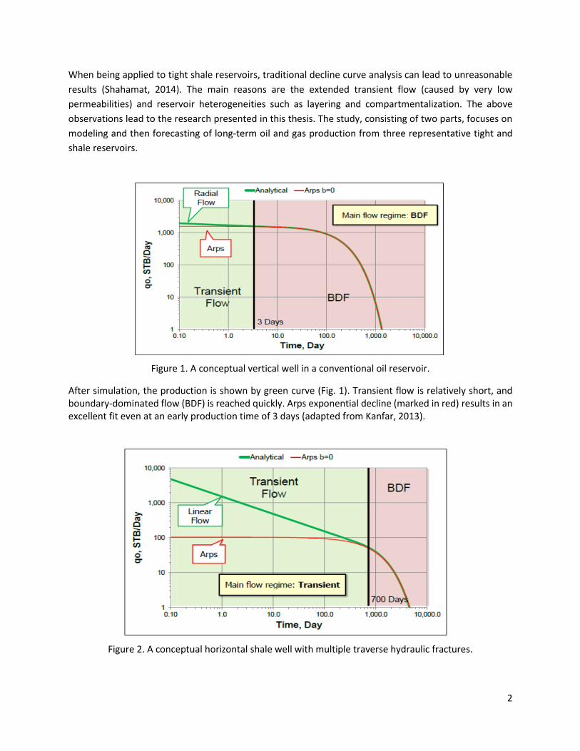
When being applied to tight shale reservoirs, traditional decline curve analysis can lead to unreasonable
results (Shahamat, 2014). The main reasons are the extended transient flow (caused by very low
permeabilities) and reservoir heterogeneities such as layering and compartmentalization. The above
observations lead to the research presented in this thesis. The study, consisting of two parts, focuses on
modeling and then forecasting of long-term oil and gas production from three representative tight and
shale reservoirs.
Figure 1. A conceptual vertical well in a conventional oil reservoir.
After simulation, the production is shown by green curve (Fig. 1). Transient flow is relatively short, and boundary-dominated flow (BDF) is reached quickly. Arps exponential decline (marked in red) results in an excellent fit even at an early production time of 3 days (adapted from Kanfar, 2013).
Figure 2. A conceptual horizontal shale well with multiple traverse hydraulic fractures.

3
As for horizontal wells with hydraulic simulation, the production is shown by green curve (Fig. 2). Arps’
method (marked in red) can only fit BDF decline which does not occur until after 700 days of production
(adapted from Kanfar, 2013).
Current models used to forecast production in unconventional oil and gas formations often fail to produce
valid results. When traditional DCA models are used in shale formations, Arps b-values greater than 1 are
commonly obtained, and these values yield infinite cumulative production, which is non-physical (Okouma
et al., 2012). Additional methods have been developed to prevent the unrealistic values produced, like
truncating hyperbolic declines with exponential declines when a minimum production rate is reached.
Truncating a hyperbolic decline with an exponential decline solves some of the problems associated with
decline curve analysis, but it is not an ideal solution. The exponential decline rate used is arbitrary, and
the value picked greatly affects the results of the forecast (Clark, 2011).
1-2 RESEARCH OBJECTIVES:
The scope of this study is to identify an easy-to-use model(s) that provide reasonable long-term
forecasting production from tight and shale oil and gas reservoirs. This work will focus on determining the
best method(s) in terms of Estimated Ultimate Recovery (EUR) accuracy, goodness of fit, and ease of
matching. In addition, these methods will be compared against each other at different production times
in order to understand the effect of production time on forecasts. All methods will be benchmarked
against simulations to ensure a validation of process.
The secondary objectives of this work include identifying the strengths and weaknesses of recently
developed decline curve methods and other empirical methods.
Lastly, the results generated by the models created can be used to forecast the productions of dataset
used, thus enabling us to gain some insight to the future of unconventional plays.
1-3 PREVIOUS WORK:
Existing decline curve analyses are based on Arps equations (Arps, 1945). Developed for conventional
reservoirs, the Arps relations (hyperbolic and exponential relations) have been the standard for evaluating
EUR in petroleum engineering applications for more than 70 years. Fetkovich et al. (1996) developed
concepts for decline curve forecasting and provided a theoretical basis for the Arps equations. Li and
Horne (2003) developed a decline curve analysis based on fluid flow mechanism and discussed its
application to Kern oil fields (Reyes et al., 2004). Mattar and Anderson (2003) highlighted the strengths
and limitations of Arps decline analysis in a comprehensive methodology for the analysis of production
data. Decline curve analysis was used in evaluating well performance in a multi-well system

4
(Marhaendrajana and Blasingame, 2001). Cheng et al. (2005) used the stochastic approach to evaluate
the uncertainty in reserve estimation-based decline curve analysis.
Table 1. Arps Equation Cases
Figure 3. Comparison of exponential, hyperbolic and harmonic relations (adapted from Shin et al., 2014)
The parameters in all equations are presented in nomenclature in the end.
The application of "Decline Curve Analysis" (DCA) in unconventional reservoirs is almost always
problematic. The relations often yield ambiguous results due to invalid assumptions (e.g., existence of the
boundary-dominated flow regime, presumption of a constant bottom hole pressure).
Misapplications of the Arps' relations to production data exhibiting long-term, transient flow generally
results in significant overestimates of reserves - specifically when the hyperbolic relation is extrapolated
in an unconstrained manner, using an Arps b-value greater than 1 (Okouma et al., 2012).

5
The issues related to the use of Arps' rate decline relations have led various researchers to propose the
following various rate decline relations which attempt to properly model the time-rate behavior,
specifically early transient and transitional flow behavior: Power Law Exponential by Ilk et al. (2008),
Stretched Exponential by Valkó (2009), Logistic Growth Model by Clark et al. (2011), and Duong Model by
Duong (2011). Each method has different tuning parameters and equation forms. However, none of these
equations can be considered sufficient to forecast the production for all unconventional plays, due to the
characteristics and operational conditions of each play and the behavior of the time-rate equation. In
other words, one equation could work very well in a specific play but possibly perform poorly in another
play.
6
CHAPTER 2
GEOLOGICAL SETTINGS
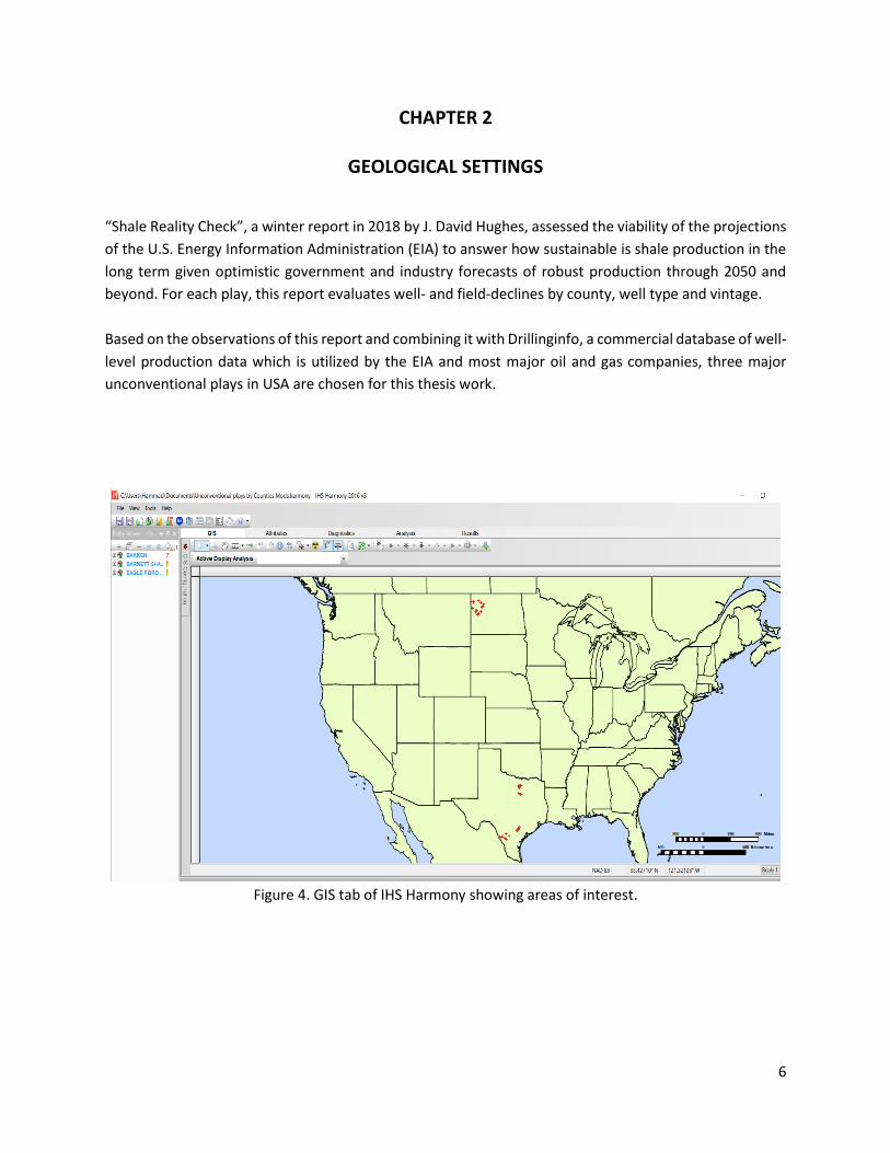
“Shale Reality Check”, a winter report in 2018 by J. David Hughes, assessed the viability of the projections
of the U.S. Energy Information Administration (EIA) to answer how sustainable is shale production in the
long term given optimistic government and industry forecasts of robust production through 2050 and
beyond. For each play, this report evaluates well- and field-declines by county, well type and vintage.
Based on the observations of this report and combining it with Drillinginfo, a commercial database of well-
level production data which is utilized by the EIA and most major oil and gas companies, three major
unconventional plays in USA are chosen for this thesis work.
Figure 4. GIS tab of IHS Harmony showing areas of interest.

7
2-1 BAKKEN PLAY
The Bakken Play in North Dakota and Eastern Montana was the first major tight oil play being developed.
The production is both from the Bakken and underlying Three Forks formations. The production rise from
nothing in 2003 to one of the largest plays in the U.S. in 2014, when it peaked. More than 13,000 wells
have been drilled, of which more than 12,000 are still producing, and this study focuses on 17 wells from
top four counties of Bakken play namely Dunn, McKenzie, Mountrail and Williams county (Fig. 5).
Figure 5. Location of 17 wells picked from top four producing counties of Bakken (ND).
2-2 BARNETT PLAY
The Barnett Play was the first major shale gas play to be developed. The production began in the mid-
1990s and grew to a peak in November 2011. More than 20,000 wells have been drilled, of which 15,000
are still producing. Drilling in the play has slowed to a near standstill, as the most productive parts of the
play are saturated with wells. The highest productivity wells are concentrated in parts of Tarrant, Johnson,
Denton, and Wise counties (Fig. 6).

8
Figure 6. Location of 20 wells picked from top four producing counties of Barnett (TX).
2-3 EAGLE FORD PLAY
The Eagle Ford Play of southern Texas rose from nothing in 2008 to be one of the largest tight oil plays in
the U.S., when it peaked in March 2015. Nearly 18,000 wells have been drilled of which more than 17,000
are still producing. The highest productivity wells occupy parts of Karnes, Dewitt, La Salle, Dimmit,
Gonzales, and McMullen counties (Fig. 7).
Figure 7. Location of 18 wells picked from top four producing counties of Eagle Ford (TX).

9
CHAPTER 3
METHODS
Harmony™ from IHS Markit is a comprehensive engineering application for analyzing oil and gas well
performance and evaluating reserves. We use this complimentary software to extract maximum value
from well performance data by creating rigorous type-wells (type curves) and forecast reserve. We assess
reserves risk with a probabilistic forecasting and run 'what If' scenarios to assess the impact of alternative
well spacing, completion design, or artificial lift mechanisms. Harmony Enterprise™ is widely used in
industry nowadays for multiphase probabilistic refracture modeling and decline auto forecast (Fig. 8).
Figure 8. Analysis tab of Harmony showing various features available per suite.
As mentioned before, DrillingInfo is used as data source for Harmony software (Figs. 9-10).

10
Figure 9. DrillingInfo page showing available tabs and services.
Figure 10. An example DrillingInfo page showing well card and available data for the picked wells.

11
The general workflow is to import monthly production data of selected wells into IHS Harmony. Then we
enter fluid and reservoir properties and wellbore data. Also incorporating pressures where available to
achieve model accuracy as close to actual conditions as possible. Next, we analyze individual wells. Using
built-in type curves, we can identify flow regimes as transient or boundary-dominated. Other diagnostic
features of IHS Harmony suite, like super position time and flowing material balance, allows us to create
a model that matches the production trend. Once we have found parameter values that match
observations and seem logical, we can then use the simulated model for forecasting. Lastly, the results of
individual wells can be combined to get the performance on reservoir level to help us compare between
various plays.
Following techniques, frequently used in the literature and industry, are employed in this study to obtain
desired results:
3-1 TYPE CURVES
Type curves provide a powerful method for analyzing pressure drawdown (flow) and buildup tests.
Fundamentally, type curves are pre-plotted solutions to the flow equations, such as the diffusivity
equation, for selected types of formations and selected initial and boundary conditions.
Because of the way they are plotted (usually on logarithmic coordinates), it is convenient to compare
actual field data plotted on the same coordinates to the type curves. The results of this comparison
frequently include qualitative and quantitative descriptions of the formation and completion properties
of the tested well.
Underlying the decline curve equations is an expectation that well-production typically follows a three-
part pattern.
1. In the initial production phase, the flow of oil or gas remains relatively steady, as pressure stays
nearly constant.
2. Next is a transient period in which the flow of oil or gas declines rapidly, as the quantity of
recoverable assets and pressure in the wellbore decreases.
3. Lastly, assets deplete to a level at which they approach the well’s defined boundaries.
Using the decline curve analysis has several shortcomings, including a probable underestimation of oil
reserves and production rates, and overestimation of reservoir performance. It also cannot account for
the likelihood of geologic changes that more-complex models may be able to include, to a certain
degree. However, the type curves are still widely in use today.

12
3-2 TYPE WELLS
Type Well is an analysis method that allows us to create a Traditional Decline or a Stretched Exponential
Decline analysis for the average of a group of wells. A Type Well analysis is performed on the group as a
whole — not on individual wells — although the forecast can be copied to the individual wells that make
up the group. Type Well forecasts are commonly applied to wells with limited or no historical production
data.
3-3 OTHER EMPIRICAL MODELS
3-3-1 Stretched Exponential Production Decline
The Stretched Exponential Decline (SEPD) method is a variation of the traditional Arps method, but is
better suited to unconventional reservoirs due to its bounded nature. One of the benefits of this method
is that for positive values of n, t, and qi, the model gives a finite value of EUR, even if no abandonment
constraints are used in time or rate.
Table 2. SEPD Equation Cases
See Appendix B for the derivation and more discussion about the Stretched Exponential Decline Model.
13
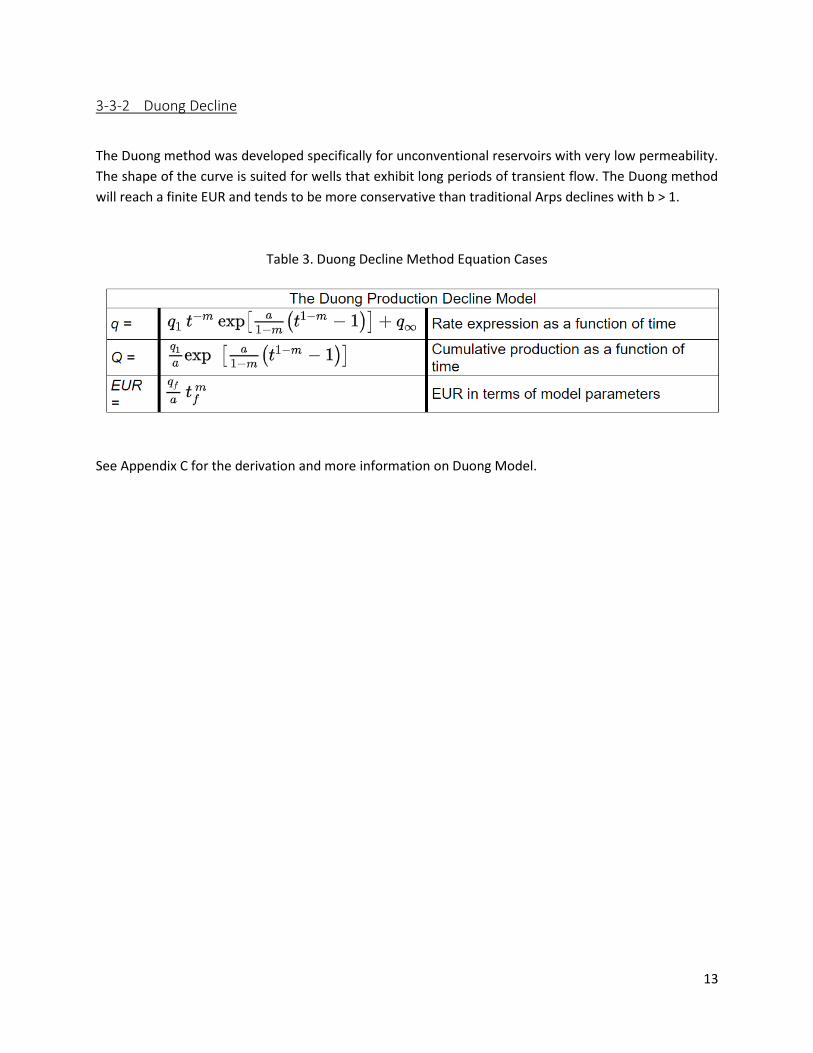
3-3-2 Duong Decline
The Duong method was developed specifically for unconventional reservoirs with very low permeability.
The shape of the curve is suited for wells that exhibit long periods of transient flow. The Duong method
will reach a finite EUR and tends to be more conservative than traditional Arps declines with b > 1.
Table 3. Duong Decline Method Equation Cases
See Appendix C for the derivation and more information on Duong Model.

14
CHAPTER 4
RESULTS
This chapter covers the findings of the study which have been subdivided into sections for easier access
and comparison.
4-1 COMPARISON OF DIFFERENT MODELS
As mentioned in the earlier sections, newer DCA methods have been introduced, mostly to model
unconventional reservoirs. Being a widely used software in industry, IHS Harmony has already
incorporated many of them. We have used our data set to generate some forecasts.
4-1-1 Gas Well Example A shale gas well from Tarrant county has been used as case study to forecast using three different DCA
models.
Arps’ Decline:
As mentioned in earlier sections, Arps’ decline curve models have been broadly used to estimate reserves
from depletion drive oil and gas reservoirs since 1945. Even now Arps decline model is used as the major
method to estimate EUR.
The Arps equation is expressed as:
where qt represents production rate at time t, qi represents stabilized rate at t=0, Di is the decline
rate at flow rate qi, and b is Arps’ decline constant.
When the production history is plotted, Harmony software can calculate decline rate and decline
constant. We would already know initial rate, so for any time t in the future, we can calculate rates
using above equation.
15
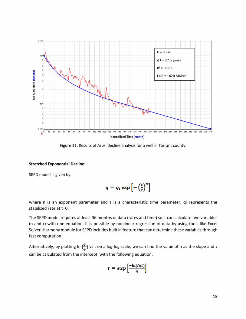
Figure 11. Results of Arps' decline analysis for a well in Tarrant county.
Stretched Exponential Decline:
SEPD model is given by:
where n is an exponent parameter and τ is a characteristic time parameter, qi represents the
stabilized rate at t=0.
The SEPD model requires at least 36 months of data (rates and time) so it can calculate two variables
(n and τ) with one equation. It is possible by nonlinear regression of data by using tools like Excel
Solver. Harmony module for SEPD includes built in feature that can determine these variables through
fast computation.
Alternatively, by plotting ln [𝑞𝑖
𝑞𝑡] vs t on a log-log scale, we can find the value of n as the slope and τ
can be calculated from the intercept, with the following equation:

16
Figure 12. Results of SEPD analysis; dashed green line is showing 20 Mscfd abandonment limit.
Duong Decline:
Duong noticed empirically that the log–log plot of q/Gp vs. t forms a straight line, and derived his model
equation as:
where a is the intercept coefficient from equation below
𝑞
𝐺𝑝= 𝑎𝑡−𝑚
m is the slope in the log–log plot and Gp is the cumulative production.
Duong method is part of the decline analysis suite of Harmony so it can automatically calculate the
constants a and m.

17
Figure 13. Results of Duong analysis
One big problem observed using Duong model is that it fails to work in boundary-dominated flow. It was
built to model wells that exhibit long transient flow. We need to have pressure data to perform flowing
material balance analysis to pin point the transition of flow regimes. Otherwise, the predicted trend will
vary greatly from the production curve trajectory in later stages of forecast.

18
Combined Plot:
Figure 14. Comparison of Arps, SEPD, and Doung models.

19
4-1-2 Oil Well Example
The oil case study uses the same approach as for gas well. The three models have been applied to an oil
well from Bakken play. The combined results are shown to avoid repetition.
Table 4. Variables Used by Three Different Models for Decline Analysis
Figure 15. Three models (Arps’, SEPD, and Duong) applied to an example of oil production.

20
Table 5. EUR Results for Different Wells by Three Different Models
EUR
Arps Decline SEPD Model Duong Model
FORGE 148-94 11B-3H 536 Mstb 397 Mstb 616 Mstb
MOUNTAIN GAP 31-10H 119 Mstb 96 Mstb 136 Mstb
THORVALD 2-6H 341 Mstb 316 Mstb 322 Mstb
EIDE 35-11R 3.5 Mstb 4.5 Mstb 6.5 Mstb
MALM 149-98-11-2-1H 337 Mstb 399 Mstb 331 Mstb
PESEK TRUST 21-26-2H 215 Mstb 253 Mstb 194 Mstb
TATTU 19-1H 391 Mstb 322 Mstb 341 Mstb
AUSTIN 1-02H 691 Mstb 596 Mstb 500 Mstb
HYNEK 5693 42-35H 265 Mstb 398 Mstb 378 Mstb
LACEY 12-10H 374 Mstb 382 Mstb 388 Mstb
SKYBOLT 1-24H 337 Mstb 604 Mstb 303 Mstb
87 WAYZETTA 111-30H 87 Mstb 80 Mstb 214 Mstb
BEAN 5703 42-34H 174 Mstb 146 Mstb 224 Mstb
BERGER 156-101-9-4-1H 203 Mstb 224 Mstb 245 Mstb
HEMSING 1 44 Mstb 43 Mstb 421 Mstb
174 LLOYD 27-1H 218 Mstb 225 Mstb 274 Mstb
BURNS, ANNA BETH 1 1943 MMscf 988 MMscf 3079 MMscf
COLE TRUST ONE "A" 1 517 MMscf 582 MMscf 550 MMscf
GRAHAM-SHOOP 1 3107 MMscf 2515 MMscf 5473 MMscf
GRIFFIN, S. H. ESTATE 1 1648 MMscf 6361 MMscf 2536 MMscf
HARDEMAN, C. J. 1 2151 MMscf 1563 MMscf 3503 MMscf
SULLIVAN, PAULINE GILL 1 1826 MMscf 2057 MMscf 2314 MMscf
ATLAS MILDRED 644 MMscf 454 MMscf 1280 MMscf
LYNE, FREDDY 1H 907 MMscf 800 MMscf 1010 MMscf
RIVER HILLS 1H 2789 MMscf 2454 MMscf 2333 MMscf
WALTON, ESTELLE 1H 2674 MMscf 2261 MMscf 2122 MMscf
BLAIR 1 2681 MMscf 2825 MMscf 2710 MMscf
CHIEF-PENT 2202 MMscf 2088 MMscf 2390 MMscf
CLEVELAND TAYLOR UNIT 1 1448 MMscf 1151 MMscf 1240 MMscf
HARMONSON, MORRIS 1 2105 MMscf 2556 MMscf 6397 MMscf
JOHNSON, LOTTIE BARTON 2 1226 MMscf 1205 MMscf 1620 MMscf
ACOLA, SAM "B" 1 1533 MMscf 1085 MMscf 1707 MMscf
LOGAN, H. H. GU 2 2991 MMscf 1624 MMscf 4524 MMscf
MILLER, WILLIAM GU B-1 5 2256 MMscf 1285 MMscf 2426 MMscf
MORRIS, ADA 5 2842 MMscf 1713 MMscf 1858 MMscf
SEWELL RANCH "A" 1-T 3055 MMscf 1686 MMscf 2553 MMscf

21
BUTLER A-304 2 305 Mstb 272 Mstb 274 Mstb
HILMER KOOPMANN A274 1 1528 Mstb 602 Mstb 2299 Mstb
MARALDO A403 1 553 Mstb 593 Mstb 707 Mstb
BEINHORN RANCH 2H 241 Mstb 207 Mstb 200 Mstb
BRISCOE CATARINA 1 36 Mstb 43 Mstb 22 Mstb
SAN PEDRO RANCH 4H 21 Mstb 20.9 Mstb 4 Mstb
BUTLER UNIT B 2 224 Mstb 212 Mstb 220 Mstb
RUNGE TOWN SITE GAS UNIT 1 1 124 Mstb 98 Mstb 150 Mstb
BROWNLOW 1H 194 Mstb 176 Mstb 185 Mstb
KILLAM GONZALEZ A 18H 2.53 Mstb 3.26 Mstb 1.97 Mstb
The above forecasts have been benchmarked with results from Drillinginfo. Stretched exponential decline
model has shown most consistent results with a least error. Usually the forecasted values are more
reserved and match P90 cases. Arps’ decline predictions are little over estimated. Duong model has shown
unstable results. They are perfect for long and less noisy data but if well performance changes during
history due to re fracking or shut in or any other reason, then the results have been highly over estimated.
4-2 DECLINE CURVES COMPARISON
4-2-1 Example of Oil Well
An oil well (CHARLIE BOB CREEK 1) from McKenzie county in Bakken play has been used to show the
workflow. Result figures along with brief description for each type curve is shown in this section.
Figure 16. Around four years of oil production data used for type curve comparison.

22
Figure 17. Fetkovich typecurve analysis (oil example)
The Fetkovich typecurves were designed for conventional oil and gas history matching. As they are based
on Arps equation, the decline coefficient is expected to be between 0 and 1.But in this case of tight oil,
the data being analyzed are still in the transient regime and have not reached the boundary dominated
flow. The model is forced to match hyperbolic decline with b=1 as it is the highest limit. The analysis still
generated EUR result of 540 Mstb but since the curve only has a goodness of fit of 0.69 with our data, we
will give less weightage to this analysis.
Fetkovich typecurves are not able to directly give original in-place volumes as some of the other analyses
do.
23
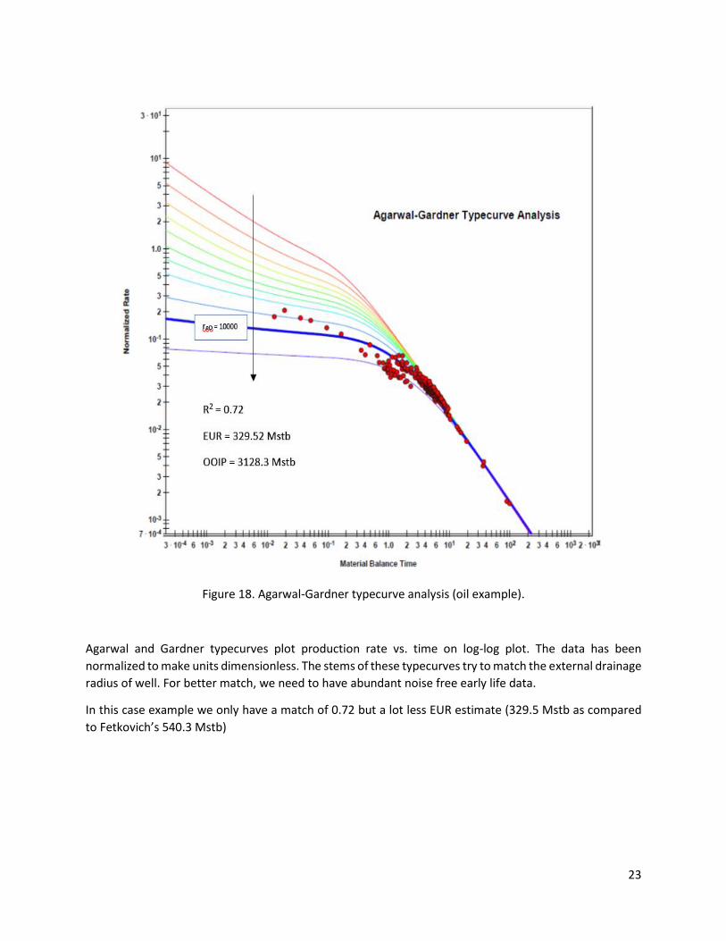
Figure 18. Agarwal-Gardner typecurve analysis (oil example).
Agarwal and Gardner typecurves plot production rate vs. time on log-log plot. The data has been
normalized to make units dimensionless. The stems of these typecurves try to match the external drainage
radius of well. For better match, we need to have abundant noise free early life data.
In this case example we only have a match of 0.72 but a lot less EUR estimate (329.5 Mstb as compared
to Fetkovich’s 540.3 Mstb)
24
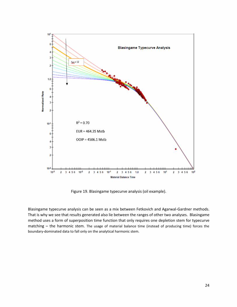
Figure 19. Blasingame typecurve analysis (oil example).
Blasingame typecurve analysis can be seen as a mix between Fetkovich and Agarwal-Gardner methods.
That is why we see that results generated also lie between the ranges of other two analyses. Blasingame
method uses a form of superposition time function that only requires one depletion stem for typecurve
matching – the harmonic stem. The usage of material balance time (instead of producing time) forces the
boundary-dominated data to fall only on the analytical harmonic stem.

25
Figure 20. Wattenbarger typecurve analysis (oil example).
Wattenbarger typecurves are particularly useful in the analysis of shale gas wells, which tend to exhibit
long-term linear flow followed by a transition towards boundary-dominated flow. To obtain information
about fracture half length, reservoir size, and well location in the reservoir, we focus on the transient
stems of typecurves. On the Wattenbarger typecurve plot, these appear on the left-side of the plot as
different ye / yw (investigated width/ reservoir width) values for the dimensionless channel model. We
select the best fitting typecurve, which provides an associated ye / yw value.
For this case study example, we don’t have width and length dimensions for well, reservoir or fractures,
so I was not able to validate the results.
Table 6. Summary of Results for Oil Case
Type Curve OOIP (Mstb) EUR (Mstb)
Agarwal-Gardner 3128.3 329.52
Blasingame 4506.1 464.35
Fetkovich 540.29
Wattenbarger 3962 792.4
26
We see drastic variations among results from different type curves. These types curves use different
approaches to estimating results. Therefore, it is very important to understand the theory behind these
analyses. The conclusion section recommends which type curve to use for which scenario. It is good
practice to combine the results from more than one model. The Drillinginfo lists the OOIP (original-oil-in
-place) for the well as 4877 Mstb and EUR as 388.7 Mstb. We will hardly ever be able to get 100 % match
using type curve analysis but using this technique, we can get a very good approximation.
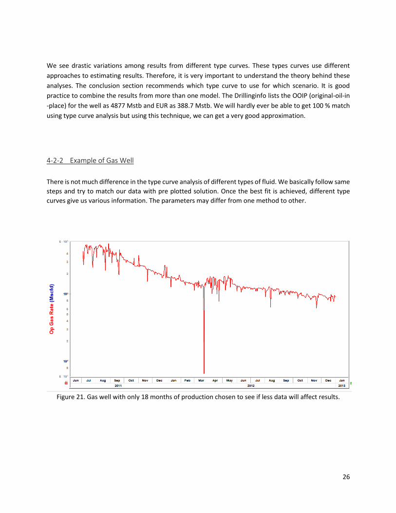
4-2-2 Example of Gas Well
There is not much difference in the type curve analysis of different types of fluid. We basically follow same
steps and try to match our data with pre plotted solution. Once the best fit is achieved, different type
curves give us various information. The parameters may differ from one method to other.
Figure 21. Gas well with only 18 months of production chosen to see if less data will affect results.

27
Figure 22. Fetkovich typecurve analysis (gas example).
Fetkovich typecurve is resulting in a poor match because it was not modelled to apply on unconventional
reservoirs. It does not provide solutions for b values greater than 1. (Fig. 24)
Figure 23. Agarwal-Gardner typecurve analysis (gas example).

28
Figure 24. Blasingame typecurve analysis (gas example).
For this particular case, the well shifted to boundary dominated flow within first few months of
production. Hence, we have less match on the transient stem side of the curve and the model is matching
data with smaller drainage radius wells (Fig.26).

29
Figure 25. Wattenbarger typecurve analysis (gas example).
Table 7. Summary of Results for Gas Case
Type Curve OGIP (MMscf) EUR (MMscf)
Agarwal-Gardner 1695 1356
Blasingame 2900 2320
Fetkovich 2561
Wattenbarger 3522 2817
Once again, we see a lot of variation among results. That is why it is very important to know our reservoir
and operating conditions as different type curves are suitable for different scenarios. They are listed in
conclusion and recommendations chapter.
Type curves also give us skin and drainage radius information along with fluid in places, which can be used
to get rough idea of ranges before carrying it to more advanced analysis and modelling

30
4-3 COUNTY COMPARISON
Within a play, the performance of top producing counties is compared by using type well technique
(introduced in Methods section). Basically, a single representative well is used for each county which has
been generated by averaging all the wells within that county.
Bakken Play:
Figure 26. Performance comparison of counties for Bakken play.
For comparison of counties in the Bakken play, we picked five wells from each county with eight years of
production data. Type-well technique has been used to represent each county by a single curve by
averaging the performance of all the wells. The forecast has been made till the wells can produce at 3 stb
per day. Results have been plotted collectively on the above figure.
Mountrail county is the most promising one for future production with the least decline and highest
returns.
31
Barnett Play:
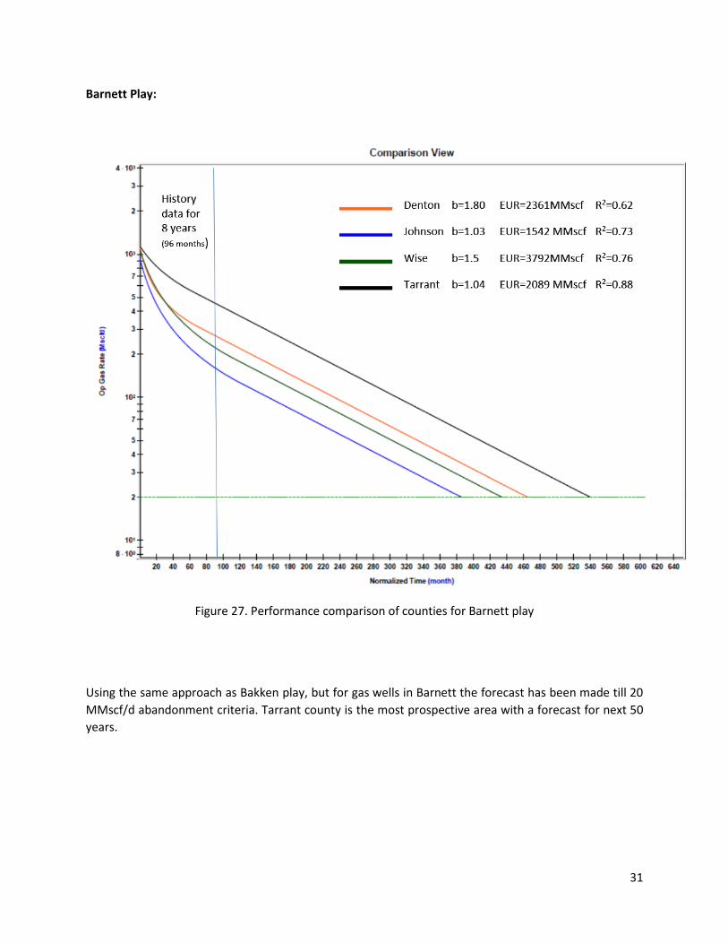
Figure 27. Performance comparison of counties for Barnett play
Using the same approach as Bakken play, but for gas wells in Barnett the forecast has been made till 20
MMscf/d abandonment criteria. Tarrant county is the most prospective area with a forecast for next 50
years.

32
Eagleford Play:
Figure 28. Performance comparison of counties for Eagle Ford play
The forecast was made till oil rates drop below 5 stb/d. The comparison plot shows the predicted
performance of top four producing counties in Eagle ford play, with the De Witt county showing the best
potential for longer future.

33
CHAPTER 5
Conclusions and Recommendations
5-1 CONCLUSIONS
Since the late 1980s, shale gas has become an important energy production component as the techniques
like horizontal well drilling and hydraulic fracturing became available. However, forecasting shale gas
production is a challenging task due to complex fracture networks and complicated mechanisms such as
gas desorption and gas slippage in shale. Even though there are many simulation methods available
including analytical models, semi-analytical models, and numerical simulation, Decline Curve Analysis has
the advantages of simplicity and efficiency for hydrocarbon production forecasting.
In this study, the most popular deterministic decline curve methods and type curve theories and analyses
are reviewed and compared with Harmony software and Drillinginfo data base.
Arps method is designed for boundary-dominated flows, but most shale gas reservoirs rarely reach the
boundary-dominated flow regime, so the original Arps curve is not appropriate to simulate the shale gas
reservoir production. As one of the earliest DCA models, Arps tends to overestimate EUR if used directly
on shale gas production.
For shale gas reservoirs with a single well produced over a sufficiently long time, the SEPD model can be
applied. The SEPD model has a better performance for transient flows than for boundary-dominated
flows. Because its expression has a finite limit, it has the advantage of providing a bounded value of EUR.
The disadvantage is that SEPD requires a sufficiently large set of production data in order to obtain good
determination of the unknown parameters. With few production data, SEPD usually return the lowest
EUR.
The Duong model is more accurate for linear flow and bilinear flow than other DCA models proposed
before. However, if the production history is shorter than 18 months, the Duong model could return
unreliable results for the EUR forecast. Most of the time, the Duong model overestimates the total EUR.
With respect to typecurves, it is noticed that Fetkovich method is the simpler one and can’t give in-place
fluid volumes but is still used as base case. Agarwal-Gardner can be used for hydraulically fractured wells
as it can estimate fracture half-length / fracture conductivity. Blasingame typecurve is found to be
effective for horizontal wells and when water drive is present. Wattenbarger typecurve is well suited for
unconventional reservoirs exhibiting long transient flows.
As far as the future of unconventional reservoirs is concerned, the simulation of models in this study has
shown favorable results. All three plays have optimistic forecasts with high recovery factors and
productions through 2050, although wells at later stages will produce at much lower rates. It is also
important to notice that DCA estimations are made on the assumption that same trends will continue in

34
future forms which is hardly the case for shale. The nature of these reservoirs is that they decline quickly,
such that production from individual wells falls 70–90% in the first three years, and field declines without
new drilling typically range 20–40% per year (Hughes, 2018). A continual investment in new drilling is
therefore required to avoid steep production declines. This will affect well spacing and many other
parameters and reservoir properties causing the forecasted results to deviate. Hence it is important to
keep updating your model periodically by adding more data. A good practice is to add production as it
becomes available at least once per month to incorporate latest changes.
5-2 RECOMMENDATIONS
The biggest disadvantage of DCA models is that most of them are empirical without a physical background.
There are potential relationships between DCA parameters and reservoir properties, which need to be
further investigated. In the future, once more information become available, more detailed investigations
about the links between DCA parameters and reservoir properties can be performed.
The combination of deterministic DCA models with machine learning techniques could also be an
interesting future trend of DCA model applications, especially with all the advancement of machine
learning and data analysis techniques.

35
APPENDICES
APPENDIX A
Arps Decline Model
The classical DCA model was proposed by Arps (1945), where the author proposed a hyperbolic function
with three parameters to simulate the decline of flow rate. In the Arps model, bottomhole pressure is
fixed, the skin factor is constant, and the flow regime is boundary-dominated flow. To derive the DCA
model, the concept of loss ratio was first introduced. The loss ratio is defined as the ratio between the
production drop of the current time step and that of the previous time step. Based on observations, Arps
proposed two different scenarios of loss ratio. The first scenario is to assume that the loss ratio is a
constant, 𝑞
𝑑𝑞𝑑𝑡
⁄= −𝑏
where b is a positive constant. Integrating above equation, we get the exponential decline functions as
follows:
q = 𝑞𝑖 𝑒−𝑡𝑏⁄
where qi is the initial rate, in bbl/day.
The second scenario is to assume that “first differences of the loss ratios are approximately constant”,
i.e.,
𝑑(𝑞
𝑑𝑞𝑑𝑡
⁄)
𝑑𝑡 = -b
The double integration of above equation allows us to obtain the rate–time relationship for hyperbolic
decline:
36
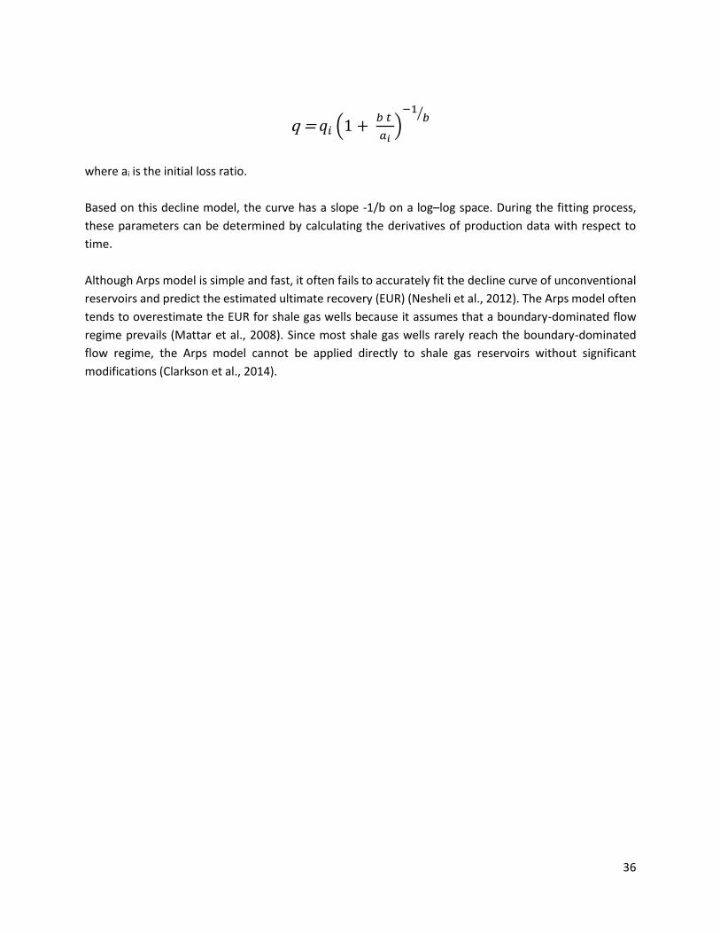
q = 𝑞𝑖 (1 + 𝑏 𝑡
𝑎𝑖)
−1𝑏⁄
where ai is the initial loss ratio.
Based on this decline model, the curve has a slope -1/b on a log–log space. During the fitting process,
these parameters can be determined by calculating the derivatives of production data with respect to
time.
Although Arps model is simple and fast, it often fails to accurately fit the decline curve of unconventional
reservoirs and predict the estimated ultimate recovery (EUR) (Nesheli et al., 2012). The Arps model often
tends to overestimate the EUR for shale gas wells because it assumes that a boundary-dominated flow
regime prevails (Mattar et al., 2008). Since most shale gas wells rarely reach the boundary-dominated
flow regime, the Arps model cannot be applied directly to shale gas reservoirs without significant
modifications (Clarkson et al., 2014).

37
APPENDIX B
Stretched Exponential Decline Model
To avoid the disadvantages of the Arps decline model and use the relatively easier access of large dataset
of well productions, Valko (2009) and Valkó and Lee (2010) proposed the Stretched Exponential Decline
Model (SEPD), in which they assume that the product rate satisfies the stretched exponential decay:
𝑑𝑞
𝑑𝑡= −𝑛 (
𝑡
𝜏)
𝑛
𝑞
𝑡
Integrating give us:
q = 𝑞𝑖 𝑒−(
𝑡
𝜏)
𝑛
where 𝜏 is the characteristic time constant and n is the exponent.
Valkó and Lee (2010) mentioned that a natural interpretation of this model is that the actual production
decline is determined by a great number of contributing volumes. All these volumes have exponential
decay rates, but with a specific distribution of characteristic time constants (𝜏).
Akbarnejad-Nesheli et al. (2012) showed that the SEPD model is advantageous for combining the concave
and convex portions of decline curves without increasing the number of model parameters and could
provide a finite (bounded) value of EUR without cutoffs in time or rate. Zuo et al. (2016) also illustrated
that the SEPD model provides a bounded EUR rather than an infinite value; moreover, the authors pointed
out that the SEPD model captures transient flow rather than boundary-dominated flow, and requires a
sufficiently long production time (usually >36 months) to accurately estimate the parameters t and n. Also,
the construction of the SEPD model requires solving complicated nonlinear equations to determine
unknown parameters

38
APPENDIX C
Duong Model
The Duong model (2011) is introduced based on one empirically derived rule, that is, the log–log plot of
q/Gp (Gp is the cumulative gas production) vs. t forms a straight line. The author conjectured that
𝑞
𝐺𝑝 = a 𝑡−𝑚
Based on above equation, the author derived the formula for well production rate and cumulative
production as follows:
𝑞 = 𝑞𝑖𝑡−𝑚 𝑎
𝑒1−𝑚 (𝑡1−𝑚 − 1)
𝐺𝑝 = 𝑞𝑖
𝑎 𝑒
𝑎1−𝑚
(𝑡1−𝑚−1)
where a is the intercept coefficient and m is the slope in the log–log plot. Kanfar and Wattenbarger (2012)
showed that the Duong model is more accurate for linear flows and bilinear–linear flows. Meyet et al.
(2013) showed that the EURs determined with PLE and Duong model vary the least with respect to the
length of production history for all wells among all of the DCA methods in their study, and other DCA
methods tend to converge towards the modified Duong model and PLE model. Furthermore, the Duong
model tends to provide the most conservative results. Zuo et al. (2016) pointed out that if m and a are
within certain ranges, the gas flow rate should decrease monotonically, and qi determination in the model
may lead to unreliable results if the production history is shorter than 18 months. Paryani et al. (2016)
fitted well with 51% of the historical production data, and the Duong model fits better with longer and
less noisy historical production data. In Wang et al. (2017), the authors proposed a new empirical method
and compared it with the SEPD model and Duong model, and concluded that the SEPD underestimates
EUR and the Duong model overestimates the ultimate recoveries.
39
APPENDIX D
Difference Between Various Typecurve Analyses
The production decline analysis techniques of Arps and Fetkovich are limited in that they do not
account for variations in bottomhole flowing pressure in the transient regime, and only account for
such variations empirically during boundary-dominated flow (by means of the empirical depletion
stems). In addition, changing pressure, volume, and temperature (PVT) properties with reservoir
pressure are not considered for gas wells.
Blasingame and his colleagues have developed a production decline method that accounts for these
phenomena. The method uses a form of superposition time function that only requires one
depletion stem for typecurve matching - the harmonic stem. One important advantage of this
method is that the typecurves used for matching are similar to those used for Fetkovich decline
analysis, without the empirical depletion stems. When the typecurves are plotted using Blasingame’s
superposition time function, the analytical exponential stem of the Fetkovich typecurve becomes
harmonic. The significance of this may not be readily evident until considering that, if the inverse of
the flowing pressure is plotted against time, pseudo-steady state depletion at a constant flow rate
follows a harmonic decline trend. In effect, Blasingame’s typecurves allow depletion at a constant
pressure to appear as if it were depletion at a constant flow rate. In fact, Blasingame et al. have
shown that boundary-dominated flow with both declining rates and pressures appear as pseudo-
steady state depletion at a constant rate, provided the rate and pressure decline monotonically.
the Fetkovich typecurves are based on combining the analytical solution to transient flow of a single-
phase fluid at a constant wellbore flowing pressure with the empirical Arps equations for boundary-
dominated flow. Fetkovich believed the exponent ‘b’ could vary between zero and one, and that it
was correlatable with fluid properties as well as recovery mechanism. Blasingame, McCray, and
Palacio developed typecurves which show the analytical transient stems along with the analytical
harmonic decline (but with the rest of the empirical hyperbolic stems absent). In addition, they
introduced two other functions; the rate integral function, and the rate integral derivative function,
which help in smoothing the often-noisy character of production data, and in obtaining a more
unique match.
40
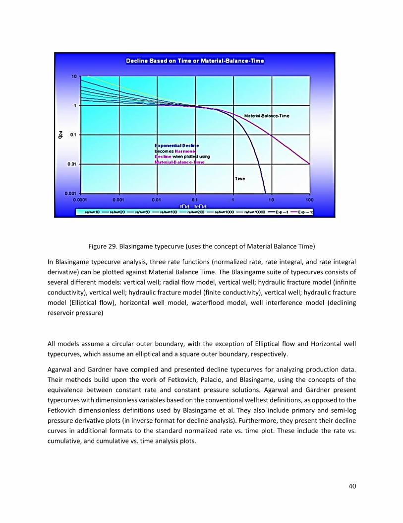
Figure 29. Blasingame typecurve (uses the concept of Material Balance Time)
In Blasingame typecurve analysis, three rate functions (normalized rate, rate integral, and rate integral
derivative) can be plotted against Material Balance Time. The Blasingame suite of typecurves consists of
several different models: vertical well; radial flow model, vertical well; hydraulic fracture model (infinite
conductivity), vertical well; hydraulic fracture model (finite conductivity), vertical well; hydraulic fracture
model (Elliptical flow), horizontal well model, waterflood model, well interference model (declining
reservoir pressure)
All models assume a circular outer boundary, with the exception of Elliptical flow and Horizontal well
typecurves, which assume an elliptical and a square outer boundary, respectively.
Agarwal and Gardner have compiled and presented decline typecurves for analyzing production data.
Their methods build upon the work of Fetkovich, Palacio, and Blasingame, using the concepts of the
equivalence between constant rate and constant pressure solutions. Agarwal and Gardner present
typecurves with dimensionless variables based on the conventional welltest definitions, as opposed to the
Fetkovich dimensionless definitions used by Blasingame et al. They also include primary and semi-log
pressure derivative plots (in inverse format for decline analysis). Furthermore, they present their decline
curves in additional formats to the standard normalized rate vs. time plot. These include the rate vs.
cumulative, and cumulative vs. time analysis plots.

41
Figure 30. Forecast Agarwal-Gardner typecurve
Wattenbarger et al. (1998) presented new typecurves to analyze the production data of the gas wells with
extended periods of linear flow. These wells are usually in very tight gas reservoirs with hydraulic fractures
designed to extend to the drainage boundary of the well.
The normalized rate and inverse semi-log pressure derivative are plotted against the material balance
time on a log-log scale of the same size as the typecurves. This plot is called the “data plot”. Any
convenient units can be used for normalized rate or time because a change in units simply caused a
uniform shift of the raw data on a logarithmic scale. It is recommended that daily operated-rates to be
plotted, and not the monthly rates; especially when transient data are analyzed.
The data plot is moved over the typecurve plot, while the axes of the two plots are kept parallel until a
good match is obtained. Several different typecurves should be tried to obtain the best fit of all the data.
The typecurve that best fits the data is selected.

42
NOMENCLATURE
Variable Description
A Area
b Decline exponent
B Formation volume factor
c Compressibility
CBM Coalbed methane
CGR Condensate Gas Ratio, bbl/MMscf, m3/103m3
d Effective decline rate
DCA Decline Curve Analysis
EUR Expected Ultimate Recovery
G Original gas-in-place
GMB Gas Material Balance
GOR Producing Gas-Oil Ratio
Ginj Cumulative gas injected
Gp Cumulative gas production
Gr Remaining gas
h Net pay
hp Perforated interval

43
Variable Description
HCPV Hydrocarbon Pore Volume
k Permeability
KB Kelly Bushing (reference point for depth measurements)
L Horizontal wellbore length
m Slope from the flow equation using material balance time
(oil)
MD Measured Depth (CF or KB)
N Original oil-in-place
Np Cumulative oil production
OGIP Original Gas-in-Place, MMscf, 106m3
OMB Oil Material Balance
OOIP Original Oil-in-Place, Mstb, 103m3
OWIP Original Water-in-Place, Mstb, 103m3
p Pressure
p̅ Average reservoir pressure
pab Abandonment pressure
pair Air pressure
paq Aquifer pressure
pbp Bubble point pressure, psi(a) or kPa(a)
PI Productivity index

44
Variable Description
PVT Pressure-Volume-Temperature
q Rate
r Radius
re Reservoir effective radius
rw Wellbore radius
RC Rate vs. cumulative production
RF Recovery factor
RR Remaining recoverable
RT Rate vs. time
Rs Solution gas-oil ratio, scf/bbl, m3/m3
s Skin
Sg Gas saturation
So Oil saturation
Sw Water saturation
t Time
T Temperature
TVD True Vertical Depth
V Volume
VHCP Hydrocarbon pore volume

45
Variable Description
WDI Water Drive Index
WOR Water-Oil Ratio
Wp Cumulative water production
xf Fracture half-length
Xe Reservoir length
Y Distance of investigation at time t
Ye Reservoir width
Z Gas compressibility factor
μ Viscosity of primary fluid (gas/oil/water)
ρ Density of fluid or rock
σ Interfacial tension (capillary pressure)
Effective horizontal stress (CBM properties)
φ Porosity
46
REFERENCES
Akbarnejad-Nesheli, B., P. Valko and J.W. Lee, 2012. Relating fracture network characteristics to shale gas
reserve estimation. In Proceedings of the SPE Americas Unconventional Resources Conference,
Pittsburgh, PA, USA, 5–7 June 2012.
Arps, J.J. 1945. Analysis of Decline Curves. Transactions of the American Institute of Mining, Metallurgical
and Petroleum Engineers (Trans AIME) 160, 228-247.
Arps, J.J. 1956. Estimation of Primary Oil Reserves. Transactions of AIME 207, 182-191.
Bloomberg, 2017. Shale King Hamm Wants to Give Oil Forecasters a Reality Check
Clark, A.J. 2011. Decline Curve Analysis in Unconventional Resource Plays Using Logistic Growth Models.
November 17, 2017.
Clarkson, C.R., F.Qanbari and J.D.Williams, 2014. Innovative use of rate-transient analysis methods to
obtain hydraulic-fracture properties for low-permeability reservoirs exhibiting multiphase flow. The
Leading Edge, Volume 30, 1108–1122.
Drillinginfo, https://info.drillinginfo.com/
Duong, A.N. 2011. Rate-decline analysis for fracture-dominated shale reservoirs. SPE Reservoir Evaluation
& Engineering 14, 377–387.
Fetkovich, M.J. 1980. Decline Curve Analysis Using Types Curves, Journal of Petroleum Technology, June
1980, 1065-1077.
Hughes, J.D. 2014. Drilling Deeper: A Reality Check on U.S. Government Forecasts for a Lasting Tight Oil &
Shale Gas Boom (Santa Rosa, CA: Post Carbon Institute, 2014); http://shalebubble.org .
Hughes, J.D. 2018. Shale Reality Check: Drilling into the U.S. Government’s Rosy Projections for Shale Gas
& Tight Oil Production Through 2050.
Kanfar, M.S. 2013. Comparison of Empirical Decline Curve Analysis for Shale Wells. Published Masters’
Thesis at the Texas A&M University.
Kupchenko, C.L., and B.W. Gault. 2008. Tight Gas Production Performance Using Decline Curves. CIPC/SPE
Gas Technology Symposium 2008 Joint Conference. Calgary, Alberta, Canada.

47
Mattar, L., B. Gault, K. Morad, C.R. Clarkson, C.M. Freeman, D. Ilk and T.A. Blasingame, 2008. Production
analysis and forecasting of shale gas reservoirs: Case history-based approach. In Proceedings of the SPE
Shale Gas Production Conference, Fort Worth, TX, USA, 16–18 November 2008.
Montgomery, J.B., and F.M. O’Sullivan. 2017. Spatial variability of tight oil well productivity and the impact
of technology. Journal of Applied Energy, vol. 195, pages 344 -355.
Okouma, V., and D. Symmons. 2012. Practical Considerations for Decline Curve Analysis in Unconventional
Reservoirs — Application of Recently Developed Time-Rate Relations. Paper SPE 162910 presented at the
SPE Hydrocarbon, Economics, and Evaluation Symposium held in Calgary, Alberta, Canada, 24–25
September.
Paryani, M., and M. Ahmadi. 2016. Using improved decline curve models for production forecasts in
unconventional reservoirs. In Proceedings of the SPE Eastern Regional Meeting, Canton, OH, USA, 13–15
September.
Poston, S.W. and Poe, B.D. Jr. 2008. Analysis of Production Decline Curves. Society of Petroleum Engineers,
U.S.A. ISBN: 978-1-55563-144-4
Shahamat, M.S. 2014. Production Data Analysis of Tight and Shale Reservoirs. Approved Thesis by the
Graduate Committee at the University of Calgary.
Tsoularis, A. and J. Wallace. 2001. Analysis of logistic growth models. Mathematical Biosciences 179(1):
21-55.
Valkó, P.P. 2009. Assigning value to stimulation in the Barnett Shale: A simultaneous analysis of 7000 plus
production histories and well completion records. In Proceedings of the SPE Hydraulic Fracturing
Technology Conference, The Woodlands, TX, USA, 19–21 January.
Valko, P.P. and W.J. Lee. 2010. A Better Way to Forecast Production from Unconventional Gas Wells. SPE
Annual Technical Conference and Exhibition, Florence, Italy.
Wang, K., and H. Li. 2017. Predicting production and estimated ultimate recoveries for shale gas wells: A
new methodology approach. Journal of Applied Energy, Elsevier, vol. 206(C), pages 1416-1431.
Yu, S. 2013. Best Practice of Using Empirical Methods for Production Forecast and EUR Estimation in
Tight/Shale Gas Reservoirs. Paper SPE 167118 presented at the SPE Unconventional Resources
Conference, Canada, Calgary, Alberta, Canada, 5–7 November 2013.
Zuo, L.H., W. Yu. 2016. A fractional decline curve analysis model for shale gas reservoirs. International
Journal of Coal Geology, 163, 140–148.

48