1  

HIWPP non-hydrostatic dynamical core tests: Results from idealized test cases

Jeffrey Whitaker

NOAA/ESRL/PSD jeffrey.s.whitaker@noaa.gov

Background: NCEP’s current operational global atmospheric model dynamical core, the GSM, or Global Spectral Model, has been evolving in continuous use for over 30 years. The horizontal resolution of the GSM (~13-km in 2015) is approaching a grid spacing at which non-hydrostatic effects become significant. In addition, the current GSM may not be able to scale up to the size of peta-scale HPC systems. These facts will require adoption of a new atmospheric dynamical core for operational global prediction in the NWS within a decade. Since the global model touches almost every operational forecast NCEP produces, transitioning a new dynamical core (dycore) into operations is difficult and costly. Therefore, the NWS needs to ensure the new dynamical core is “future proof” and can serve NOAA’s needs for at least 20 years. The HIWPP and NGGPS projects are collaborating to evaluate candidate non-hydrostatic dynamical cores with a battery of tests. The initial phase of testing under HIWPP has been completed. Each dynamical core ran a series of idealized tests, inspired by the Dynamical Core Intercomparison Project of 2012 (DCMIP; https://earthsystemcog.org/projects/dcmip-2012). The results of these tests are summarized in this document. Participating Dynamical Cores: The five candidate dycores are listed below, with sponsors in parentheses. • FV3 (GFDL) – Cubed sphere grid, finite-volume discretization. (non-hydrostatic version of the

hydrostatic core described in Lin, 2004). • MPAS (NCAR) – Unstructured grid with C-grid variable staggering (Skamarock et al, 2012). • NEPTUNE (NRL) – Flexible cubed sphere or icosahedral grid using a spectral element

discretization with the Non-hydrostatic Unified Model of the Atmosphere (NUMA) core (Giraldo et al, 2014).

• NIM (ESRL) – Non-hydrostatic Icosahedral Model (unstaggered finite-volume A-grid implementation).

• NMMUJ (EMC) – Finite-difference cubed-sphere grid version of the B-grid lat/lon grid core described in Janjic and Gall (2012). The construction of the ‘uniform jacobian’ cubed sphere grid is described in NCEP office note 467, available at http://www.lib.ncep.noaa.gov/ncepofficenotes/2010s/.

Idealized Tests:

  2  

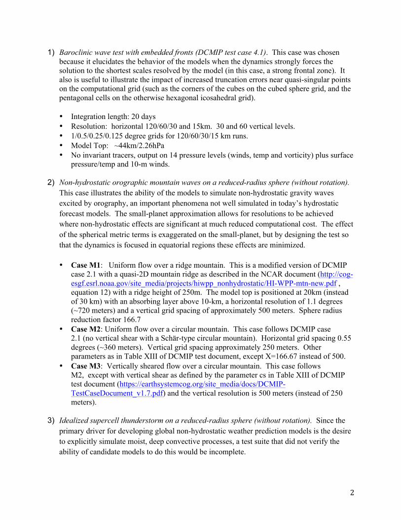
1) Baroclinic wave test with embedded fronts (DCMIP test case 4.1). This case was chosen because it elucidates the behavior of the models when the dynamics strongly forces the solution to the shortest scales resolved by the model (in this case, a strong frontal zone). It also is useful to illustrate the impact of increased truncation errors near quasi-singular points on the computational grid (such as the corners of the cubes on the cubed sphere grid, and the pentagonal cells on the otherwise hexagonal icosahedral grid).

• Integration length: 20 days • Resolution: horizontal 120/60/30 and 15km. 30 and 60 vertical levels. • 1/0.5/0.25/0.125 degree grids for 120/60/30/15 km runs. • Model Top: ~44km/2.26hPa • No invariant tracers, output on 14 pressure levels (winds, temp and vorticity) plus surface

pressure/temp and 10-m winds.

2) Non-hydrostatic orographic mountain waves on a reduced-radius sphere (without rotation). This case illustrates the ability of the models to simulate non-hydrostatic gravity waves excited by orography, an important phenomena not well simulated in today’s hydrostatic forecast models. The small-planet approximation allows for resolutions to be achieved where non-hydrostatic effects are significant at much reduced computational cost. The effect of the spherical metric terms is exaggerated on the small-planet, but by designing the test so that the dynamics is focused in equatorial regions these effects are minimized.

• Case M1: Uniform flow over a ridge mountain. This is a modified version of DCMIP case 2.1 with a quasi-2D mountain ridge as described in the NCAR document (http://cog-esgf.esrl.noaa.gov/site_media/projects/hiwpp_nonhydrostatic/HI-WPP-mtn-new.pdf , equation 12) with a ridge height of 250m. The model top is positioned at 20km (instead of 30 km) with an absorbing layer above 10-km, a horizontal resolution of 1.1 degrees (~720 meters) and a vertical grid spacing of approximately 500 meters. Sphere radius reduction factor 166.7

• Case M2: Uniform flow over a circular mountain. This case follows DCMIP case 2.1 (no vertical shear with a Schär-type circular mountain). Horizontal grid spacing 0.55 degrees (~360 meters). Vertical grid spacing approximately 250 meters. Other parameters as in Table XIII of DCMIP test document, except X=166.67 instead of 500.

• Case M3: Vertically sheared flow over a circular mountain. This case follows M2, except with vertical shear as defined by the parameter cs in Table XIII of DCMIP test document (https://earthsystemcog.org/site_media/docs/DCMIP-TestCaseDocument_v1.7.pdf) and the vertical resolution is 500 meters (instead of 250 meters).

3) Idealized supercell thunderstorm on a reduced-radius sphere (without rotation). Since the primary driver for developing global non-hydrostatic weather prediction models is the desire to explicitly simulate moist, deep convective processes, a test suite that did not verify the ability of candidate models to do this would be incomplete.

  3  

• Convection is initiated with a warm bubble in a convectively unstable sounding in vertical shear on a non-rotating reduced-radius sphere (with a reduction factor of 120).

• Detailed specification in the document (http://cog-esgf.esrl.noaa.gov/site_media/projects/hiwpp_nonhydrostatic/Supercell-testcase.pdf) provided by NCAR.

• Two hour integrations at 4, 2, 1 and 0.5 km horizontal resolution.

Numerical diffusion parameters were not part of the test case specification, instead each modeling group chose diffusion parameters independently as they saw fit.

Baroclinic wave test results:

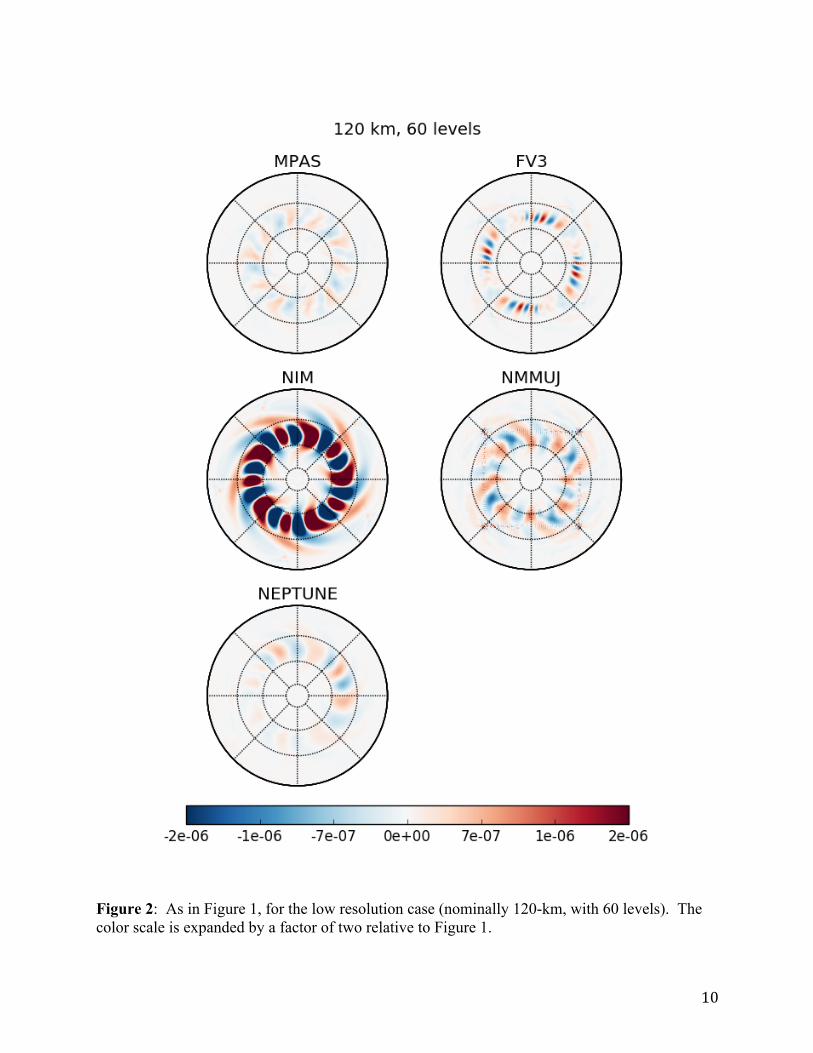
A baroclinic wave packet grows from a very small amplitude perturbation on an unstable zonal jet, reaching an amplitude at which nonlinear effects are strong and frontal collapse is well underway by day 9. The initial perturbation is applied in the Northern Hemisphere only, so the growth of instabilities in the Southern Hemisphere is due primarily to discretization errors at day 9. Figures 1 and 2 show the Southern Hemisphere 850 hPa vorticity, with the zonal mean removed to emphasize the grid imprinting signal, for each of the five models at the highest and lowest horizontal resolutions. Only the 60 level results are shown, since the 30 level results are qualitatively similar.

The level of grid imprinting varies among the models, but is generally larger in the lower resolution case. The NEPTUNE model has very little grid imprinting at 15-km resolution, while NIM has a relatively larger signal on the coarsest (120-km) resolution but is comparable to MPAS and FV3 on the finest (15-km) resolution This is consistent with the order of accuracy used in the numerics, NIM and NMMUJ being 2nd order, while the other models employ 3rd or 4th order schemes. Models with higher-order numerics have better numerical consistency across the ‘special’ points on the grid (the eight cube corners on the cubed sphere grid or the 12 pentagonal grid cells on the icosahedral grid). The locations of the cube corners in the cubed sphere grid are evident in the FV3 and NMMUJ solutions, and wavenumber 5 and 10 patterns (excited by increased truncation error at the pentagonal grid cells) are evident in both NIM and MPAS solutions. It is important to note that the amplitude of the Southern Hemisphere vorticity in this case is not only proportional to variations in the truncation error at the quasi-singular points of the computational grid, but is also related to how those patterns of error project on the fastest growing modes of the unstable baroclinic jet.

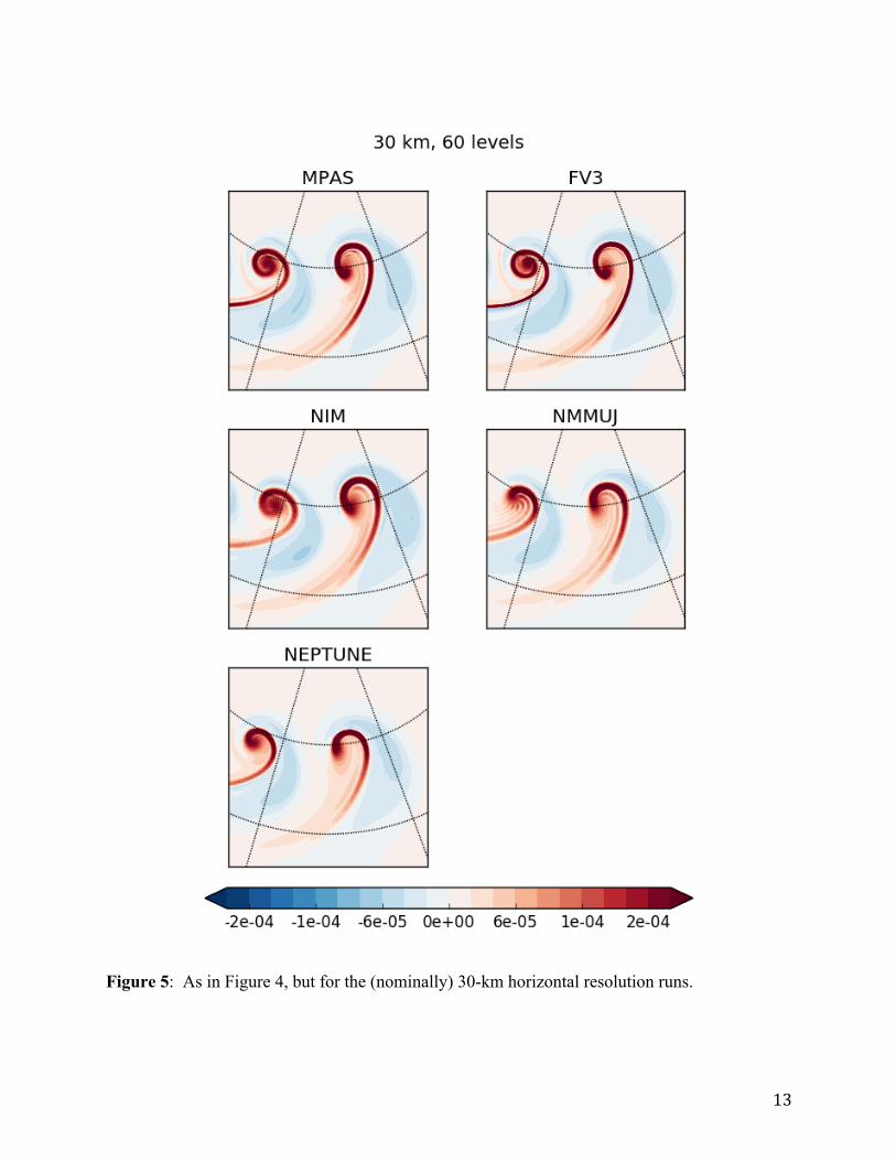
Figure 3 shows the 850hPa relative vorticity in the Northern Hemisphere day 9 for the high-resolution case. All of the models create a large amplitude baroclinic wave packet, with strong fronts evident, but at this scale it is hard to see any differences between the solutions. Zooming in on the strongest frontal zone (Figures 4-7), reveals some interesting differences. The location of the cyclones is similar in the MPAS and FV3 solutions, while the NIM solution is displaced slightly eastward, and the NEPTUNE and NMMUJ solutions slightly westward, relative to the other solutions. It is not clear whether this is due to differences in the model numeric and diffusion, differences in the placement of vertical levels, or small errors in the specification of

  4  

the initial state.1 An independent calculation was performed with a version of the hydrostatic spectral GFS dynamical core at 60-km resolution (not shown), and the phasing of the cyclones at day 9 agreed with the MPAS and FV3 solutions. However, since this case has no analytic solution, it is not known definitively which model is most accurate with regard to the phasing of the cyclones. The MPAS and FV3 solutions are generally very similar. The NMMUJ solution exhibits banding structure in the vorticity field around the fronts, which is particularly noticeable at 60 km resolution. The NEPTUNE, NMMUJ and NIM solutions appear to be more heavily damped than the MPAS and FV3 solutions at the coarser resolutions (see e.g. Figure 7).

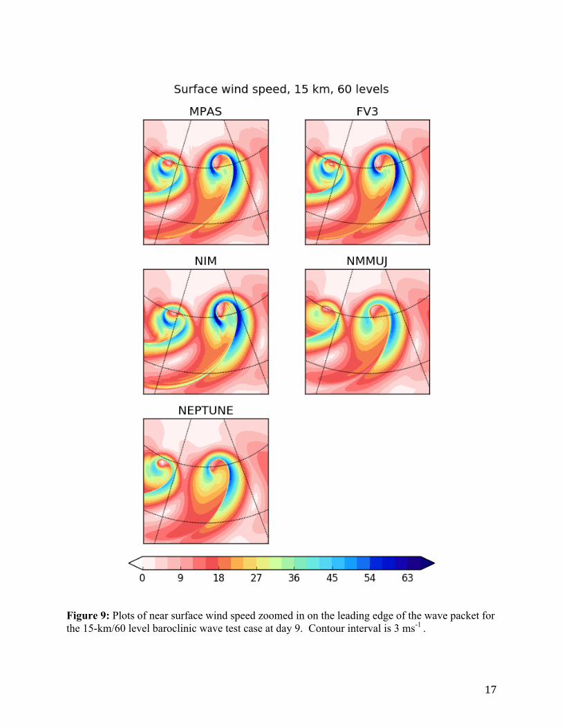
Figure 8 shows the global kinetic-energy spectrum as a function of total wavenumber (ranging from wavenumber 20 to wavenumber 1440), computed using spherical harmonic transforms of the lowest model level horizontal wind components. The spectrum is computed for day 9 of the 15-km/60 level solutions. Two reference lines are plotted on the figure, one showing the slope of a -3 power law spectrum (consistent with two-dimension turbulence theory) and one showing the slope of a -5/3 power law spectrum (consistent with fully three-dimensional turbulence). The wavelengths corresponding to two and four times the nominal grid resolution are also indicated as vertical lines. All of the models exhibit a spectrum shallower (steeper) than would be expected from two-dimension (three-dimensional) turbulence theory at larger scales, and a relatively steep spectrum at shorter scales (due to the effects of numerical dissipation). The relative sharpness of the drop-off in the spectra at the shortest wavelengths is proportional to strength and scale of the numerical dissipation in each model. The MPAS and FV3 spectra are similar, with slightly more damping near the truncation scale in MPAS, and slightly more energy at wavelengths near four times the grid resolution. The NMMUJ solution is clearly the most heavily damped, followed by NEPTUNE. The NIM spectrum exhibits a peak at a wavelength close to four times the grid resolution. This is associated with banding structure in the surface wind speed just behind the cold front (Figure 9). The smoothness of the surface wind field in the NEPTUNE and NMMUJ solution seen in Figure 9 is consistent with the spectra shown in Figure 8. FV3 appears to best represent the frontal discontinuity, with the least noise near the grid scale behind the cold front.

Orographic mountain wave test results:

Figure 10 shows vertical cross sections along the equator for test case M1, a quasi two-dimensional ridge in barotropic, solid-body rotation flow on a reduced radius sphere (with a dry isothermal atmosphere). This is a modification of the circular mountain DCMIP test case (M2) that allows for more direct comparison with published solutions for a flow over infinite two-dimensional ridges in Cartesian geometry (see e.g. Schär et al, 2002 and Klemp et al, 2003). Also shown in Figure 10 is the linear analytic solution for an infinite ridge on a flat plane. The gravity waves forced by this terrain have two dominant components: a larger-scale hydrostatic wave that is characterized by deep vertical propagation, and smaller-scale waves generated by the smaller scale terrain variations and characterized by rapid decay with height due to non-hydrostatic effects. With the exception of NMMUJ, all of the solutions agree qualitatively with the analytic solution, indicating that the model solutions are essentially linear at the equator, and

                                                                                                               1  The NIM developers did find and correct a bug in the initial condition specification for this case. The corrected results are shown. This reduced, but did not eliminate the eastward phase shift.

  5  

the spherical metric terms are small, even on the reduced radius sphere. The NMMUJ solution appears unrealistic, as it does for all the reduced-radius sphere test cases.

Horizontal maps of vertical velocity at the model level closest to 8 km are shown in Figure 11. There is no analytic solution for the behavior away from the equator in this case, since the analytic solution assumes no meridional variation on a flat plane. The meridional propagation of wave energy is broadly similar in the MPAS and FV3 solutions. NIM displays some grid- scale numerical noise in the extra-tropics because it does not use any artificial dissipation in this test case (besides whatever numerical diffusion is inherent to the spatial discretization). NEPTUNE exhibits stronger meridional propagation and stronger wave activity in the polar regions than the other models.

Figure 12 shows vertical cross sections along the equator for test case M2, a circular mountain centered on the equator in an isothermal atmosphere with barotropic, solid-body rotation flow. This is identical to the DCMIP test case 2.1, except that that the sphere reduction factor was reduced from 500 to 166.7 to minimize the impact of the spherical metric terms and to prevent disturbances from circling the globe by the end of the two-hour integration. The analytic solution computed for flat-plane geometry is shown for reference. The gravity waves forced by this terrain have two primary components: a larger-scale hydrostatic wave that is characterized by nearly vertical propagation (similar to the M1 solution), and smaller-scale non-hydrostatic waves that propagate vertically and downstream. The same small-scale shallow non-hydrostatic trapped waves just above the terrain evident in the M1 solution are also present. Since the model top is placed higher in this test case, the solutions are show up to 20 km instead of 10 km. The primary differences seen in the model solutions are associated with the non-hydrostatic downstream propagating waves. MPAS, FV3 and NIM produce qualitatively similar solutions on the equator, which agree well with the flat-plane linear analytic solution. NEPTUNE more strongly attenuates the waves in the downstream direction. However, NEPTUNE is the only model that uses the deep atmosphere equation set, which likely explains differences with the other models (all of which use a shallow atmosphere approximation).2 A solution computed with a halved sphere reduction factor (83.33 instead of 166.7) is in better agreement with the other models, with less downstream wave attenuation (Figure 13).

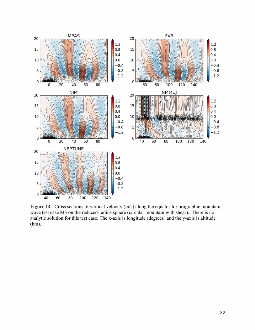
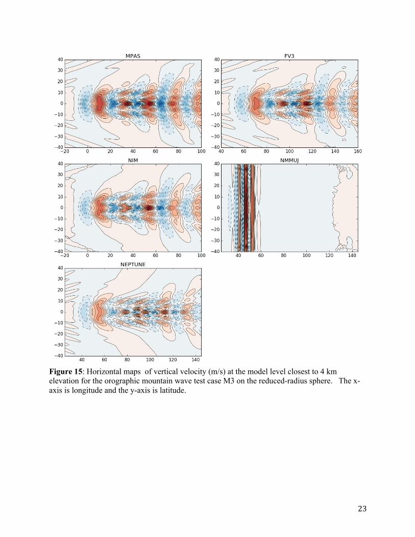
Case M3 is identical to case M2, except that the zonal flow includes vertical shear. This presence of stronger winds aloft traps the shorter wavelength components of the mountain waves in the lower atmosphere below the level where they become evanescent. The trapped waves become ducted and propagate horizontally downstream. There is no linear analytic flat-plane solution for this case. As for M1 and M2, the MPAS, FV3 and NIM solutions are all very similar along the equator (Figure 14). The NEPTUNE solution is different than the other models, primarily in the phase propagation of the waves. This may be related to the fact that NEPTUNE does not use the shallow atmosphere approximation. There is much less meridional propagation of wave activity in this case relative to M1 (Figure 15).

                                                                                                               2  In a deep-atmosphere model, the radial distance from the center of the earth (r) is not assumed to be constant; this appears in terms inversely proportional to r in the momentum equations (White et. al. 2005). On a reduced-radius sphere, this can have a significant effect since the depth of the atmosphere is the same order as the radius of the planet.

  6  

Idealized supercell test results:

This is an important test case, because it demonstrates the ability of the dynamical cores to simulate deep moist convection realistically. The ability to simulate deep moist convection explicitly is the primary motivation for developing global non-hydrostatic models. Here a very simple microphysics scheme is used (the warm rain microphysics scheme described in Kessler (1969)). The microphysical processes included are: the production, fall and evaporation of rain, the accretion and autoconversion of cloud water, the production of cloud water from condensation, and the effect of water loading on buoyancy. Each of the modeling groups implemented the same simple FORTRAN subroutine, provided by NCAR, to compute the warm- rain microphysics. Following the approach developed by Weisman and Klemp (1982) to simulate the basic characteristics of observed supercell thunderstorms, a warm bubble is initialized on the equator of a reduced radius sphere in a horizontally homogenous convective unstable environment characterized by large CAPE (~2200 m2s-2) and linear vertical wind shear below 5 km. No boundary layer processes are included, and the models employ a free-slip lower boundary condition plus horizontal and vertical diffusion. As in all the other tests, each modeling group chose diffusion parameters independently.

The expected evolution (based upon Weisman and Klemp (1982) and many other similar idealized numerical studies) is the rapid development of a convective updraft, followed by splitting along the north and south flanks of the original storm’s outflow boundary, producing two identical storms that propagate to the right and left of the mean shear vector.

Figure 16 shows time series of the maximum vertical velocity for each of the models. Separate lines are shown for each of the four horizontal resolutions (500-m, 1-km, 2-km and 4-km). All of the models (except NMMUJ) produce strong convective updrafts within 30 minutes, exceeding 30-50 meters per second at the highest resolution. The time step used in the 4-km and 2-km NIM runs was set to 2 seconds, which is identical to the 500-m run, otherwise significant updrafts did not form. NEPTUNE also used a time step of 2 seconds for all resolutions. MPAS used a 4-km time step of 24 seconds, FV3 20 seconds and NMMUJ 8 seconds. NMMUJ does not produce any coherent convective updrafts, the large vertical velocities seen in Figure 16 are associated with grid-scale noise, primarily near the poles.

Figures 17-20 show horizontal maps of vertical velocity at the model level closest to 2500 meters, 90 minutes into the integration. At this time, splitting of the original updraft has completed and all the models except NMMUJ show identical convective updrafts north and south of the equator at the higher resolutions. NMMUJ does not produce any coherent updrafts at all. The other models produce qualitatively similar solutions at 500-m, 1-km and 2-km resolutions. The FV3 solution is somewhat smoother than the other models, since FV3 group chose higher diffusion parameters to produce a nearly-converged solution at the highest resolution. The MPAS solution is the only one that produces a rear-flank downdraft just upstream of the main updraft. At the coarsest resolution (4-km), the convective updrafts are marginally resolved. MPAS, FV3 and NIM still produce solutions that retain the basic structure of the split cells present at the higher resolutions, but the NEPTUNE solution is qualitatively different from the higher-resolution solutions.

  7  

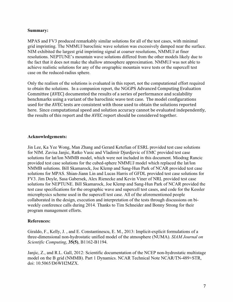
Summary:

MPAS and FV3 produced remarkably similar solutions for all of the test cases, with minimal grid imprinting. The NMMUJ baroclinic wave solution was excessively damped near the surface. NIM exhibited the largest grid imprinting signal at coarser resolutions, NMMUJ at finer resolutions. NEPTUNE’s mountain wave solutions differed from the other models likely due to the fact that it does not make the shallow atmosphere approximation. NMMUJ was not able to achieve realistic solutions for any of the orographic mountain wave tests or the supercell test case on the reduced-radius sphere.

Only the realism of the solutions is evaluated in this report, not the computational effort required to obtain the solutions. In a companion report, the NGGPS Advanced  Computing  Evaluation  Committee  (AVEC)  documented  the  results  of  a  series  of  performance  and  scalability  benchmarks  using  a  variant  of  the  baroclinic  wave  test  case.    The  model  configurations  used  for  the  AVEC  tests  are  consistent  with  those  used  to  obtain  the  solutions  reported  here.    Since  computational  speed  and  solution  accuracy  cannot  be  evaluated  independently,  the  results  of  this  report  and  the  AVEC  report  should  be  considered  together.  

Acknowledgements:

Jin Lee, Ka Yee Wong, Man Zhang and Gerard Ketefian of ESRL provided test case solutions for NIM. Zavisa Janjic, Ratko Vasic and Vladimir Djurdjevic of EMC provided test case solutions for lat/lon NMMB model, which were not included in this document. Miodrag Rancic provided test case solutions for the cubed-sphere NMMUJ model which replaced the lat/lon NMMB solutions. Bill Skamarock, Joe Klemp and Sang-Hun Park of NCAR provided test case solutions for MPAS. Shian-Jiann Lin and Lucas Harris of GFDL provided test case solutions for FV3. Jim Doyle, Sasa Gabersek, Alex Rienecke and Kevin Viner of NRL provided test case solutions for NEPTUNE. Bill Skamarock, Joe Klemp and Sang-Hun Park of NCAR provided the test case specifications for the orographic wave and supercell test cases, and code for the Kessler microphysics scheme used in the supercell test case. All of the aforementioned people collaborated in the design, execution and interpretation of the tests through discussions on bi- weekly conference calls during 2014. Thanks to Tim Schneider and Bonny Strong for their program management efforts.

References:

Giraldo, F., Kelly, J. , and E. Constantinescu, E. M., 2013: Implicit-explicit formulations of a three-dimensional non-hydrostatic unified model of the atmosphere (NUMA). SIAM Journal on Scientific Computing, 35(5), B1162-B1194.

Janjic, Z., and R.L. Gall, 2012: Scientific documentation of the NCEP non-hydrostatic multistage model on the B grid (NMMB). Part 1 Dynamics. NCAR Technical Note NCAR/TN-489+STR, doi: 10.5065/D6WH2MZX.

  8  

Kessler, E., 1969: On the distribution and continuity of water substance in atmospheric circulation. Meteor. Monogr., No. 32, Amer. Meteor. Soc., 84pp.

Klemp, J. B., W. Skamarock, and O. Fuhrer, 2003: Numerical consistency of metric terms in terrain-following coordinates. Mon. Wea. Rev., 131, 1229-1239.

Lin, S.-J., 2004: A vertically Lagrangian Finite-Volume Dynamical Core for Global Models. Mon. Wea. Rev., 132, 2293-2307.

Michalakes, J. and co-authors, 2015: AVEC Report: NGGPS Level-1 Benchmarks and Software Evaluation. 22 pages, available from author upon request (john.michalakes@noaa.gov).

Schär, C., D. Leuenberger, O. Fuhrer, D. Lüthi, and C. Girard, 2002: A new terrain-following vertical coordinate formulation for atmospheric prediction models, Mon. Wea. Rev., 130, 2459–2480.

Skaramarock, W, M. Duda, L. Fowler, S.-.H Park and T. Ringler, 2012: A Multi-scale Nonhydrostatic Atmospheric Model Using Centroidal Voronoi Tesselations and C-Grid Staggering. Mon. Wea. Rev., 240, 3090-3105, doi:10.1175/MWR-D-11-00215.1

Weisman, M. L., and J. B. Klemp, 1982: The dependence of numerically simulated convective storms on vertical wind shear and buoyancy. Mon. Wea. Rev., 110, 504–520.

White, A. A., B. J. Hoskins, and A. Staniforth, 2005: Consistent approximate models of the global atmosphere: shallow, deep, hydrostatic, quasi-hydrostatic and non-hydrostatic. Quarterly Journal of the Royal Meteorological Society, 131, 2081-2107, doi: 10.1256/qj.04.49.

  9  

Figure 1: Plots of Southern Hemisphere relative vorticity at 850hPa (with the zonal mean removed) for the high-resolution (nominally 15-km, with 60 levels) baroclinic wave test case at day 9. The outer edge of the plot is 20 degrees south latitude.

  10  

Figure 2: As in Figure 1, for the low resolution case (nominally 120-km, with 60 levels). The color scale is expanded by a factor of two relative to Figure 1.

  11  

Figure 3: Plots of Northern Hemisphere relative vorticity at 850hPa for the high-resolution (nominally 15-km, with 60 levels) baroclinic wave test case at day 9. Contour interval is 1 x 10-4 s-1 . The outer edge of the plot is 20 degrees north latitude.

  12  

Figure 4: Plots of relative vorticity at 850hPa zoomed in on the leading edge of the wave packet for the high-resolution (nominally 15-km, with 60 vertical levels) baroclinic wave test case at day 9. Contour interval is 1 x 10-4 s-1 .

  13  

Figure 5: As in Figure 4, but for the (nominally) 30-km horizontal resolution runs.

  14  

Figure 6: As in Figure 4, but for the (nominally) 60-km horizontal resolution runs.

  15  

Figure 7: As in Figure 4, but for the (nominally) 120-km horizontal resolution runs.

  16  

Figure 8: Near surface global kinetic energy spectra (m2/s2) for day 9 of the 15-km/60 level baroclinic wave test case solutions. The x-axis is wavelength in km, with values ranging from total wavenumber 20 (~ 2000 km) to wavenumber 1440 (~ 28 km), with a log-scale in total wavenumber. Two reference lines are plotted, one with a slope corresponding to a -3 power-law spectrum (solid black), and one with a slope corresponding to a -5/3 power-law spectrum. The two vertical lines represent wavelengths corresponding to two and four times the nominal grid resolution (30 km and 60 km).

  17  

Figure 9: Plots of near surface wind speed zoomed in on the leading edge of the wave packet for the 15-km/60 level baroclinic wave test case at day 9. Contour interval is 3 ms-1 .

  18  

  Figure 10: Cross sections of vertical velocity (m/s) along the equator for orographic mountain wave test case M1 on the reduced-radius sphere (quasi-2D ridge in a barotropic zonal flow). The x-axis is longitude (degrees) and the y-axis is altitude (km). The plot in the lower right corner is the analytical solution for the flat plane with a infinite ridge, excerpted from the test case description provided by NCAR, and available on the HIWPP web site (http://cog-esgf.esrl.noaa.gov/site_media/projects/hiwpp_nonhydrostatic/HI-WPP-mtn-new.pdf).

  19  

Figure 11: Horizontal maps of vertical velocity (m/s) at the model level closest to 8 km elevation for the orographic mountain wave test case M1 on the reduced-radius sphere. The x-axis is longitude and the y-axis is latitude.

  20  

Figure 12: Cross sections of vertical velocity (m/s) along the equator for orographic mountain wave test case M2 on the reduced-radius sphere (circular mountain in a barotropic zonal flow). The x-axis is longitude (degrees) and the y-axis is altitude (km). The plot in the lower right corner is the analytical solution for the flat plane, excerpted from the test case description provided by NCAR, and available on the HIWPP web site (http://cog-esgf.esrl.noaa.gov/site_media/projects/hiwpp_nonhydrostatic/HI-WPP-mtn-new.pdf).

  21  

Figure 13: As in Figure 11 for the NEPTUNE solution, except computed on a sphere with doubled radius.

  22  

Figure 14: Cross sections of vertical velocity (m/s) along the equator for orographic mountain wave test case M3 on the reduced-radius sphere (circular mountain with shear). There is no analytic solution for this test case. The x-axis is longitude (degrees) and the y-axis is altitude (km).

  23  

Figure 15: Horizontal maps of vertical velocity (m/s) at the model level closest to 4 km elevation for the orographic mountain wave test case M3 on the reduced-radius sphere. The x-axis is longitude and the y-axis is latitude.

  24  

Figure 16: Time series of the maximum vertical velocity for the supercell test case on the reduced radius sphere. Separate lines for each model represent the four different horizontal resolutions run (500-m, 1-km, 2-km and 4-km).

  25  

Figure 17: Horizontal maps of vertical velocity (m/s) on the model level nearest 2.5 km for the supercell test case on the reduced radius sphere, for the 500-m resolution solution. The y-axis is latitude, and the x-axis is longitude.

  26  

Figure 18: As in Figure 17, for the 1-km resolution runs.

  27  

Figure 19: As in Figure 17, for the 2-km resolution runs.

  28  

Figure 20: As in Figure 17, for the 4-km resolution runs.