HMMER3 beta test: User’s GuideBiological sequence analysis using profile hidden Markov models

http://hmmer.org/Version 3.0b3; November 2009

Sean R. EddyJanelia Farm Research CampusHoward Hughes Medical Institute

19700 Helix DriveAshburn VA 20147 USAhttp://eddylab.org/

Copyright (C) 2009 Howard Hughes Medical Institute.

Permission is granted to make and distribute verbatim copies of this manual provided the copyright noticeand this permission notice are retained on all copies.

HMMER is licensed and freely distributed under the GNU General Public License version 3 (GPLv3). For acopy of the License, see http://www.gnu.org/licenses/.

HMMER is a trademark of the Howard Hughes Medical Institute.

1

Contents

1 Introduction 3Design goals of HMMER3 . . . . . . . . . . . . . . . . . . . . . . . . . . . . . . . . . . . . . . . . . 3What made it into the HMMER3.0 test code . . . . . . . . . . . . . . . . . . . . . . . . . . . . . . . 4What’s still missing . . . . . . . . . . . . . . . . . . . . . . . . . . . . . . . . . . . . . . . . . . . . . 5What I hope to accomplish in testing . . . . . . . . . . . . . . . . . . . . . . . . . . . . . . . . . . . 5

2 Installation 7Quick installation instructions . . . . . . . . . . . . . . . . . . . . . . . . . . . . . . . . . . . . . . . 7System requirements . . . . . . . . . . . . . . . . . . . . . . . . . . . . . . . . . . . . . . . . . . . 7Multithreaded parallelization for multicores by default . . . . . . . . . . . . . . . . . . . . . . . . . . 8MPI parallelization for clusters is optional . . . . . . . . . . . . . . . . . . . . . . . . . . . . . . . . 9Using build directories . . . . . . . . . . . . . . . . . . . . . . . . . . . . . . . . . . . . . . . . . . . 9Makefile targets . . . . . . . . . . . . . . . . . . . . . . . . . . . . . . . . . . . . . . . . . . . . . . . 9

3 Tutorial 11Files used in the tutorial . . . . . . . . . . . . . . . . . . . . . . . . . . . . . . . . . . . . . . . . . . 11Searching a sequence database with a single profile HMM . . . . . . . . . . . . . . . . . . . . . . 11

Step 1: build a profile HMM with hmmbuild . . . . . . . . . . . . . . . . . . . . . . . . . . . . . 11Step 2: search the sequence database with hmmsearch . . . . . . . . . . . . . . . . . . . . . 13

Searching a profile HMM database with a query sequence . . . . . . . . . . . . . . . . . . . . . . . 19Step 1: create an HMM database flatfile . . . . . . . . . . . . . . . . . . . . . . . . . . . . . . 19Step 2: compress and index the flatfile with hmmpress . . . . . . . . . . . . . . . . . . . . . . 20Step 3: search the HMM database with hmmscan . . . . . . . . . . . . . . . . . . . . . . . . 20

Creating multiple alignments with hmmalign . . . . . . . . . . . . . . . . . . . . . . . . . . . . . . . 21Single sequence queries using phmmer . . . . . . . . . . . . . . . . . . . . . . . . . . . . . . . . . 22Iterative searches using jackhmmer . . . . . . . . . . . . . . . . . . . . . . . . . . . . . . . . . . . 23

4 File formats 25HMMER profile HMM files . . . . . . . . . . . . . . . . . . . . . . . . . . . . . . . . . . . . . . . . . 25

header section . . . . . . . . . . . . . . . . . . . . . . . . . . . . . . . . . . . . . . . . . . . . 25main model section . . . . . . . . . . . . . . . . . . . . . . . . . . . . . . . . . . . . . . . . . . 27

Stockholm, the recommended multiple sequence alignment format . . . . . . . . . . . . . . . . . . 28syntax of Stockholm markup . . . . . . . . . . . . . . . . . . . . . . . . . . . . . . . . . . . . 29semantics of Stockholm markup . . . . . . . . . . . . . . . . . . . . . . . . . . . . . . . . . . 29recognized #=GF annotations . . . . . . . . . . . . . . . . . . . . . . . . . . . . . . . . . . . . 30recognized #=GS annotations . . . . . . . . . . . . . . . . . . . . . . . . . . . . . . . . . . . . 30recognized #=GC annotations . . . . . . . . . . . . . . . . . . . . . . . . . . . . . . . . . . . . 30recognized #=GR annotations . . . . . . . . . . . . . . . . . . . . . . . . . . . . . . . . . . . . 31

2

1 Introduction

This is a user’s guide to the HMMER3 test distribution.It really isn’t meant for a new user. I will assume you are already familiar with profile hidden Markov

models (profile HMMs) (Krogh et al., 1994; Eddy, 1998; Durbin et al., 1998); with the previous versionof HMMER [HMMER2, http://hmmer.org]; with other popular biological sequence comparison tools,such as BLAST (Altschul et al., 1997); and with running sequence analysis tools on a UNIX or UNIX-likecommand line. If this isn’t true of you, you should probably not be using the HMMER3 code yet. Instead,you should wait for a later and more stable version, when the user documentation will take less for granted.

Design goals of HMMER3

HMMER3’s objective is to combine the power of probabilistic inference with high computational speed. Weaim to upgrade some of molecular biology’s most important sequence analysis applications to use morepowerful statistical inference engines, without sacrificing computational performance.

Specifically, HMMER3 has three main design features that, in combination, distinguish it from previoustools:

Explicit representation of alignment uncertainty. Most sequence alignment analysis tools report only asingle best-scoring alignment. However, sequence alignments are uncertain, and the more distantlyrelated sequences are, the more uncertain alignments become. HMMER3 calculates complete pos-terior alignment ensembles rather than single optimal alignments. Posterior ensembles get used fora variety of useful inferences involving alignment uncertainty. For example, any HMMER3 sequencealignment is accompanied by posterior probability annotation, representing the degree of confidencein each individual aligned residue.

Sequence scores, not alignment scores. Alignment uncertainty has an important impact on the power ofsequence database searches. It’s precisely the most remote homologs – the most difficult to identifyand potentially most interesting sequences – where alignment uncertainty is greatest, and where thestatistical approximation inherent in scoring just a single best alignment breaks down the most. Tomaximize power to discriminate true homologs from nonhomologs in a database search, statisticalinference theory says you ought to be scoring sequences by integrating over alignment uncertainty,not just scoring the single best alignment. HMMER3’s log-odds scores are sequence scores, not justoptimal alignment scores; they are integrated over the posterior alignment ensemble.

Speed. A major limitation of previous profile HMM implementations (including HMMER2) was their slowperformance. HMMER3 implements a new heuristic acceleration algorithm. For most queries, it’sabout as fast as BLAST.

Individually, none of these points is new. As far as alignment ensembles and sequence scores go, prettymuch the whole reason why hidden Markov models are so theoretically attractive for sequence analysis isthat they are good probabilistic models for explicitly dealing with alignment uncertainty. The SAM profileHMM software from UC Santa Cruz has always used full probabilistic inference (the HMM Forward andBackward algorithms) as opposed to optimal alignment scores (the HMM Viterbi algorithm). HMMER2 hadthe full HMM inference algorithms available as command-line options, but used Viterbi alignment by default,in part for speed reasons. Calculating alignment ensembles is even more computationally intensive thancalculating single optimal alignments.

One reason why it’s been hard to deploy sequence scores for practical large-scale use is that we haven’tknown how to accurately calculate the statistical significance of a log-odds score that’s been integratedover alignment uncertainty. Accurate statistical significance estimates are essential when one is trying todiscriminate homologs from millions of unrelated sequences in a large sequence database search. Thestatistical significance of optimal alignment scores can be calculated by Karlin/Altschul statistics (Karlin and

3

Altschul, 1990, 1993). Karlin/Altschul statistics are one of the most important and fundamental advancesintroduced by BLAST. However, this theory doesn’t apply to integrated log-odds sequence scores (HMM“Forward scores”). The statistical significance (expectation values, or E-values) of HMMER3 sequencescores is determined by using recent theoretical conjectures about the statistical properties of integratedlog-odds scores which have been supported by numerical simulation experiments (Eddy, 2008).

And as far as speed goes, there’s really nothing new about HMMER3’s speed either. Besides Kar-lin/Altschul statistics, the main reason BLAST has been so useful is that it’s so fast. Our design goal inHMMER3 was to achieve rough speed parity between BLAST and more formal and powerful HMM-basedmethods. The acceleration algorithm in HMMER3 is a new heuristic. It seems likely to be more sensitivethan BLAST’s heuristics on theoretical grounds. It certainly benchmarks that way in practice (Eddy, 2009,manuscript in preparation). Additionally, it’s very well suited to modern hardware architectures. We expectto be able to take good advantage of GPUs and other parallel processing environments in the near future.

What made it into the HMMER3.0 test codeSingle sequence queries: new to HMMER3

phmmer Search a sequence against a sequence database. (BLASTP-like)jackhmmer Iteratively search a sequence against a sequence database. (PSIBLAST-like)

Replacements for HMMER2’s functionality

hmmbuild Build a profile HMM from an input multiple alignment.hmmsearch Search a profile HMM against a sequence database.hmmscan Search a sequence against a profile HMM database.hmmalign Make a multiple alignment of many sequences to a common profile HMM.

Other utilities

hmmconvert Convert profile formats to/from HMMER3 format.hmmemit Generate (sample) sequences from a profile HMM.hmmfetch Get a profile HMM by name or accession from an HMM database.hmmpress Format an HMM database into a binary format for hmmscan.hmmstat Show summary statistics for each profile in an HMM database.

The quadrumvirate of hmmbuild/hmmsearch/hmmscan/hmmalign replaces HMMER2’s core functional-ity of hmmbuild/hmmsearch/hmmpfam/hmmalign in people’s domain analysis and annotation pipelines, forinstance using profile databases like Pfam or SMART. These four programs have already been subjectedto some serious independent testing by Rob Finn of the Pfam Consortium, who visited Janelia for severalmonths in order to adopt HMMER3 at Pfam, apparently by beating the living tar out of it. I haven’t yet fixedall the issues the evil Rob has identified, but I have fixed the showstopping bugs.1

The phmmer and jackhmmer programs are new to HMMER3. They searches a single sequence againsta sequence database, akin to BLASTP and PSIBLAST, respectively. (Internally, they just produce a profileHMM from the query sequence, then run HMM searches.)

In the Tutorial section, I’ll show examples of running each of these programs, using examples in thetutorial/ subdirectory of the distribution.

1I think.

4

What’s still missing

Oh, lots. The most egregious lacunae include:More processor support. One of the attractive features of the MSV algorithm is that it is a very tight

and efficient piece of code, which ought to be able to take advantage of recent advances in using massivelyparallel GPUs (graphics processing units), and other specialized processors such as the Cell processor, orFPGAs. We have prototype work going on in a variety of processors, but none of this is far along as yet.But this work (combined with the parallelization) is partly why we expect to wring significant more speed outof HMMER in the future.

More speed. Even on x86 platforms, HMMER3’s acceleration algorithms are still on a nicely slopingbit of their asymptotic optimization curve. I still think I can accelerate the code by another two-fold or so.Additionally, for a small number of HMMs (< 1% of Pfam models), the acceleration core is performingrelatively poorly, for reasons I pretty much understand (having to do with biased composition; most of thesepesky models are hydrophobic membrane proteins), but which are nontrivial to work around. This’ll producean annoying behavior that some testers are sure to notice: if you look systematically, sometimes you’ll seea model that runs at something more like HMMER2 speed, 100x or so slower than an average query. This,needless to say, Will Be Fixed.

DNA sequence comparison. HMMER’s search pipeline is somewhat specialized to protein/proteincomparison: specifically, the pipeline works by filtering individual sequences, winnowing down to a subsetof the sequences in a database that need close attention from the full heavy artillery of Bayesian inference.This strategy doesn’t work for long DNA sequences; it doesn’t filter the human genome much to say “there’sa hit on chromosome 1”. The algorithms need to be adapted to identify high-scoring regions of a targetsequence, rather than filtering by whole sequence scores. (You can chop a DNA sequence into overlappingwindows and HMMER3 would work fine on such a chopped-up database, but that’s a disgusting kludge andI don’t want to know about it.)

Translated comparisons. We’d of course love to have the HMM equivalents of BLASTX, TBLASTN,and TBLASTX. They’ll come.

More sequence input formats. HMMER3 will work fine with FASTA files for unaligned sequences, andStockholm files for multiple sequence alignments. It has parsers for a handful of other formats (Genbank,EMBL, and Uniprot flatfiles; SELEX format alignments) that we’ve tested somewhat. It’s particularly missingparsers for some widely used alignment formats such as Clustal format, so using HMMER3 on the MSAsproduced by many popular multiple alignment programs (MUSCLE or MAFFT for example) is harder than itshould be, because it requires a reformat to Stockholm format.

More alignment modes. HMMER3 only does local alignment. HMMER2 also could do glocal alignment(align a complete model to a subsequence of the target) and global alignment (align a complete model to acomplete target sequence). The E-value statistics of glocal and global alignment remain poorly understood.HMMER3 relies on accurate significance statistics, far more so than HMMER2 did, because HMMER3’sacceleration pipeline works by filtering out sequences with poor P-values.

Part of the reason for the test phase is to confirm that these points are just as annoying to you as they areto me, and therefore important to fix asap. Feel free to tell me you want these things even though I alreadyknow about them. I also want to find out what glaring problems you find that I’m not already losing sleepover. (Really.)

What I hope to accomplish in testing

The core of HMMER3’s functionality seems stable to me, but all the stuff wrapped around it – the stuffyou see, like the applications, command line options, i/o formats – is prototypical and still fluid. The mainobjective of the test period is for a small number of savvy power users to have the opportunity to givefeedback while the user-oriented layers of HMMER3 are still under development – in particular, before its

5

basic feature set, command line options, and input and output formats get frozen. You might want it to spitout XML, or you like tab-delimited format, or you want this number or that number on such-and-such a lineto make it really fit in your analysis pipeline, or you really really need a command line option for slowing thesearch programs back down to HMMER2 speed so you have more time for coffee2. This is the kind of stuffI’d most like to hear now while the code is still fluid.

An obvious corollary of this responsiveness to your feedback is, don’t write any heavy duty outputparsers around HMMER3 just yet. You should expect all the output formats to change, at least slightly,before a public release is finalized.

Of course, since it’s test code, I’d like to also hear about bugs: how you manage to break it, or when itproduces inconsistent, wrong, or confusing results, or when it doesn’t compile or run at all. Some bugs, Ialready know about, but I’d still like to hear about them just to know you care.

Cryptogenomicon (http://cryptogenomicon.org/) is a blog where I’ll be talking about issues asthey arise in HMMER3, and where you can comment or follow the discussion.

2Actually, this option already exists: --max.

6

2 Installation

Quick installation instructions

Download hmmer-3.0b3.tar.gz from http://hmmer.org/, or directly from ftp://selab.janelia.org/pub/software/hmmer3/hmmer-3.0b3.tar.gz; untar; and change into the newly created direc-tory hmmer-3.0b3:

> wget ftp://selab.janelia.org/pub/software/hmmer3/hmmer-3.0b3.tar.gz> tar xf hmmer-3.0b3.tar.gz> cd hmmer-3.0b3

The beta test code includes precompiled binaries for x86/Linux platforms. These are in the binaries

directory. You can just stop here if you like, if you’re on a x86/Linux machine and you want to try theprograms out without installing them.

To compile new binaries from source, do a standard GNUish build:> ./configure> make

To compile and run a test suite to make sure all is well, you can optionally do:> make check

All these tests should pass.You don’t have to install HMMER programs to run them. The newly compiled binaries are now in the

src directory; you can run them from there. To install the programs and man pages somewhere on yoursystem, do:

> make installBy default, programs are installed in /usr/local/bin and man pages in /usr/local/man/man1/.

You can change /usr/local to any directory you want using the ./configure --prefix option, as in./configure --prefix /the/directory/you/want.

If you have the Intel C compiler icc, we strongly recommend that you use it (instead of gcc, for example),for performance reasons, by specifying CC=icc either in your environment or on the > ./configurecommand line.

For example, on our systems, we would do:> ./configure CC=icc LDFLAGS=-static --prefix=/usr/local/hmmer-3.0/> make> make check> make install

That’s it. You can keep reading if you want to know more about customizing a HMMER3 installation, oryou can skip ahead to the next chapter, the tutorial.

System requirements

Operating system: HMMER is designed to run on POSIX-compatible platforms, including UNIX, Linuxand MacOS/X. The POSIX standard essentially includes all operating systems except Microsoft Windows.1

The alpha test code includes precompiled binaries for Linux. These were compiled with the Intel Ccompiler (icc) on an x86 64 Intel platform running Red Hat Enterprise Linux AS4. We believe they shouldbe widely portable to different Linux systems.

We have tested most extensively on Linux, and to a lesser extent on MacOS/X. We aim to be portableto all other POSIX platforms. We currently do not develop or test on Windows.

1There are add-on products available for making Windows more POSIX-compliant and more compatible with GNU-ish configuresand builds. One such product is Cygwin, http:www.cygwin.com, which is freely available. Although we do not test on Windowsplatforms, we understand HMMER builds fine in a Cygwin environment on Windows.

7

Processor: HMMER3 depends on vector parallelization methods that are supported on most modernprocessors. H3 requires either an x86-compatible (IA32/IA64) processor that supports the SSE2 vectorinstruction set, or a PowerPC processor that supports the Altivec/VMX instruction set. SSE2 is supportedon Intel processors from Pentium 4 on, and AMD processors from K8 (Athlon 64) on; we believe thisincludes almost all Intel processors since 2000 and AMD processors since 2003. Altivec/VMX is supportedon Motorola G4, IBM G5, and IBM Power6 processors, which we believe includes almost all PowerPC-baseddesktop systems since 1999 and servers since 2007.

If your platform does not support one of these vector instruction sets, the configure script will revert toan unoptimized implementation called the “dummy” implementation. This implementation is two orders ofmagnitude slower. It will enable you to see H3’s features on a much wider range of processors, but is notsuited for real production work.

We do aim to be portable to all modern processors. The acceleration algorithms are designed to beportable despite their use of specialized SIMD vector instructions. We hope to add support for the SunSPARC VIS instruction set, for example. We believe that the code will be able to take advantage of GP-GPUs and FPGAs in the future.

Compiler: The source code is C, conforming to POSIX and ANSI C99 standards. It should compile withany ANSI C99 compliant compiler, including the GNU C compiler gcc. We test the code using both the gcc

and icc compilers.If you compile HMMER from source, we strongly recommend using the Intel C compiler icc rather than

gcc. icc is free for noncommercial use and heavily discounted for academic use. GNU gcc generatesHMMER3 code that is significantly slower than icc code.2 If you find yourself saying, hey, those guys saidthis program’s supposed to be as fast as BLAST, but it only seems half as fast – odds are you recompiledfrom source with gcc.

Libraries and other installation requirements: HMMER includes a software library called Easel, whichit will automatically compile during its installation process. By default, HMMER3 does not require anyadditional libraries to be installed by you, other than standard ANSI C99 libraries that should already bepresent on a system that can compile C code. Bundling Easel instead of making it a separate installationrequirement is a deliberate design decision to simplify the installation process.3

One of the objectives of the alpha test is to identify portability issues. If HMMER3 fails to compile and/or runfast under a POSIX-compliant OS, on an x86 or PowerPC processor that supports SSE2 or Altivec/VMX,using an ANSI C99-compliant compiler, please report the problem. If it fails at all (with the portable “dummy”implementation) on any POSIX/ANSI C99 compatible platform regardless of processor type, please reportthe problem.

Multithreaded parallelization for multicores by default

The four search programs support multicore parallelization. This is implemented using POSIX threads. Bydefault, the configure script will identify whether your platform supports POSIX threads (almost all platformsdo), and will automatically compile in multithreading support.

If you want to disable multithreading at compile time, recompile from source after giving the --disable-threads

flag to ./configure.2Bjarne Knudsen has identified what’s probably the main reason, and it’s not gcc’s fault. We’ll be able to address the speed

difference in the near future.3If you install more than one package that uses the Easel library, it may become an annoyance; you’ll have multiple instantiations of

Easel lying around. The Easel API is not yet stable enough to decouple it from the applications that use it, like HMMER and Infernal.

8

By default, the search programs will use all available cores on your machine. You can control thenumber of cores each HMMER process will use with the --cpu <x> command line option or the HMMER NCPU

environment variable. Accordingly, you should observe about a 2x or 4x speedup on dual-core or quad-coremachines, relative to previous releases. Even with a single CPU (--cpu 1), HMMER will devote a separateexecution thread to database input, resulting in significant speedup over serial execution.

If you specify --cpu 0, the program will run in serial-only mode, with no threads. This might be useful ifyou suspect something is awry with the threaded parallel implementation.

MPI parallelization for clusters is optional

The four search programs and hmmbuild now also support MPI (Message Passing Interface) parallelizationon clusters. To use MPI, you first need to have an MPI library installed, such as OpenMPI (www.open-mpi.org).

MPI support is not enabled by default, and it is not compiled into the precompiled binaries that we supplywith HMMER. To enable MPI support at compile time, give the --enable-mpi option to the ./configure

command.To use MPI parallelization, each program that has an MPI-parallel mode has an --mpi command line

option. This option activates a master/worker parallelization mode. (Without the --mpi option, if you runa program under mpirun on N nodes, you’ll be running N independent duplicate commands, not a singleMPI-enabled command. Don’t do that.)

It’s highly advantageous to get mpicc to use the Intel C compiler rather than its default, which is of-ten gcc. Different MPI distributions may have different ways of selecting the C compiler and its options.OpenMPI can be controlled by environment variables. For example, in our environment, we currently buildHMMER3 for MPI using:

> setenv OMPI CC "icc"> setenv OMPI CFLAGS "-O3"> ./configure --enable-mpi --prefix=/usr/local/hmmer3> make

Using build directories

The installation process from source now supports using separate build directories, using the GNU-standardVPATH mechanism. This allows you to maintain separate builds for different processors or with differentconfiguration/compilation options. All you have to do is run the configure script from the directory you wantto be the root of the build directory. For example:

> mkdir my-hmmer-build> cd my-hmmer-build> /path/to/hmmer/configure> make

You’d probably only use this feature if you’re a developer, maintaining several different builds for testingpurposes.

Makefile targets

all Builds everything. Same as just saying make.

check Runs automated test suites in both HMMER and the Easel library.

clean Removes all files generated by compilation (by make). Configuration (files generated by ./configure)is preserved.

9

distclean Removes all files generated by configuration (by ./configure) and by compilation (by make).

Note that if you want to make a new configuration (for example, to try an MPI version by./configure --enable-mpi; make) you should do a make distclean (rather than a make

clean), to be sure old configuration files aren’t used accidentally.

10

3 Tutorial

Here’s a tutorial walk-through of some small projects with HMMER3. This should suffice to get you orientedto a “safe path” through HMMER3 alpha test code that should work as advertised – before you start boldlyexploring later-to-be-documented command line options that might or might not be doing anything sensibleyet.

Files used in the tutorial

The subdirectory /tutorial in the HMMER distribution contains the files used in the tutorial, as well as anumber of examples of various file formats that HMMER reads. The important files for the tutorial are:

globins4.sto An example alignment of four globin sequences, in Stockholm format. This align-ment is a subset of a famous old published structural alignment from Don Bashford(Bashford et al., 1987).

globins4.hmm An example profile HMM file, built from globins4.sto, in HMMER3 ASCII textformat.

globins4.out An example hmmsearch output file that results from searching the globins4.hmm

against Uniprot 15.7.

fn3.sto An example alignment of 106 fibronectin type III domains. This is the Pfam 22.0 fn3

seed alignment. It provides an example of a Stockholm format with more complexannotation. We’ll also use it for an example of hmmsearch analyzing sequencescontaining multiple domains.

fn3.hmm A profile HMM created from fn3.sto by hmmbuild.

7LESS DROME A FASTA file containing the sequence of the Drosophila Sevenless protein, a recep-tor tyrosine kinase whose extracellular region is thought to contain seven fibronectintype III domains.

fn3.out Output of hmmsearch fn3.hmm 7LESS DROME.

Pkinase.sto The Pfam 22.0 Pkinase seed alignment of protein kinase domains.

minifam An example HMM flatfile database, containing three models: globins4, fn3, andPkinase.

minifam.h3{m,i,f,p} Binary compressed files corresponding to minifam, produced by hmmpress.

HBB HUMAN A FASTA file containing the sequence of human β−hemoglobin, used as an exam-ple query for phmmer and jackhmmer.

Searching a sequence database with a single profile HMM

Step 1: build a profile HMM with hmmbuild

HMMER starts with a multiple sequence alignment file that you provide. Currently HMMER3 only readsStockholm alignments.1 The file tutorial/globins4.sto is an example of a simple Stockholm file. Itlooks like this:

1I’m lying. It can read more. I just don’t trust its other parsers yet.

11

# STOCKHOLM 1.0

HBB_HUMAN ........VHLTPEEKSAVTALWGKV....NVDEVGGEALGRLLVVYPWTQRFFESFGDLSTPDAVMGNPKVKAHGKKVLHBA_HUMAN .........VLSPADKTNVKAAWGKVGA..HAGEYGAEALERMFLSFPTTKTYFPHF.DLS.....HGSAQVKGHGKKVAMYG_PHYCA .........VLSEGEWQLVLHVWAKVEA..DVAGHGQDILIRLFKSHPETLEKFDRFKHLKTEAEMKASEDLKKHGVTVLGLB5_PETMA PIVDTGSVAPLSAAEKTKIRSAWAPVYS..TYETSGVDILVKFFTSTPAAQEFFPKFKGLTTADQLKKSADVRWHAERII

HBB_HUMAN GAFSDGLAHL...D..NLKGTFATLSELHCDKL..HVDPENFRLLGNVLVCVLAHHFGKEFTPPVQAAYQKVVAGVANALHBA_HUMAN DALTNAVAHV...D..DMPNALSALSDLHAHKL..RVDPVNFKLLSHCLLVTLAAHLPAEFTPAVHASLDKFLASVSTVLMYG_PHYCA TALGAILKK....K.GHHEAELKPLAQSHATKH..KIPIKYLEFISEAIIHVLHSRHPGDFGADAQGAMNKALELFRKDIGLB5_PETMA NAVNDAVASM..DDTEKMSMKLRDLSGKHAKSF..QVDPQYFKVLAAVIADTVAAG.........DAGFEKLMSMICILL

HBB_HUMAN AHKYH......HBA_HUMAN TSKYR......MYG_PHYCA AAKYKELGYQGGLB5_PETMA RSAY.......//

Most popular alignment formats are similar block-based formats, and can be turned into Stockholmformat with a little editing or scripting. Don’t forget the # STOCKHOLM 1.0 line at the start of the alignment,nor the // at the end. Stockholm alignments can be concatenated to create an alignment database flatfilecontaining many alignments.

The hmmbuild command builds a profile HMM from an alignment (or HMMs for each of many alignmentsin a Stockholm file), and saves the HMM(s) in a file. For example, type:

> hmmbuild globins4.hmm tutorial/globins4.stoand you’ll see some output that looks like:

# hmmbuild :: profile HMM construction from multiple sequence alignments# HMMER 3.0b3 (November 2009); http://hmmer.org/# Copyright (C) 2009 Howard Hughes Medical Institute.# Freely distributed under the GNU General Public License (GPLv3).# - - - - - - - - - - - - - - - - - - - - - - - - - - - - - - - - - - - -# input alignment file: globins4.sto# output HMM file: globins4.hmm# - - - - - - - - - - - - - - - - - - - - - - - - - - - - - - - - - - - -

# idx name nseq alen mlen eff_nseq re/pos description#---- -------------------- ----- ----- ----- -------- ------ -----------1 globins4 4 171 149 0.96 0.589

# CPU time: 0.55u 0.00s 00:00:00.55 Elapsed: 00:00:00.56

If your input file had contained more than one alignment, you’d get one line of output for each model. Forinstance, a single hmmbuild command suffices to turn a Pfam seed alignment flatfile (such as Pfam-A.seed)into a profile HMM flatfile (such as Pfam.hmm).

The information on these lines is almost self-explanatory. The globins4 alignment consisted of 4 se-quences with 171 aligned columns. HMMER turned it into a model of 149 consensus positions, whichmeans it defined 22 gap-containing alignment columns to be insertions relative to consensus. The 4 se-quences were only counted as an “effective” total sequence number (eff nseq) of 0.96. The model endedup with a relative entropy per position ((re/pos; information content) of 0.589 bits.

This output format is rudimentary. HMMER3 knows quite a bit more information about what it’s doneto build this HMM. Some of this information is likely to be useful to you, the user. As H3 testing anddevelopment proceeds, we’re likely to expand the amount of data that hmmbuild reports.

The new HMM was saved to globins4.hmm. If you were to look at this file (and you don’t have to – it’sintended for HMMER’s consumption, not yours), you’d see something like:

HMMER3/b [3.0b3 | November 2009]NAME globins4LENG 149ALPH aminoRF noCS noMAP yesDATE Sat Nov 14 10:47:39 2009NSEQ 4EFFN 0.964844

12

CKSUM 2027839109STATS LOCAL MSV -9.9014 0.70957STATS LOCAL VITERBI -10.7224 0.70957STATS LOCAL FORWARD -4.1637 0.70957HMM A C D E F G H I ... W Y

m->m m->i m->d i->m i->i d->m d->dCOMPO 2.36614 4.52553 2.96662 2.70479 3.20868 3.02051 3.41129 2.90113 ... 4.55399 3.62918

2.68640 4.42247 2.77497 2.73145 3.46376 2.40504 3.72516 3.29302 ... 4.58499 3.615250.57544 1.78073 1.31293 1.75577 0.18968 0.00000 *

1 1.70038 4.17733 3.76164 3.36686 3.72281 3.29583 4.27570 2.40482 ... 5.32720 4.10031 9 - -2.68618 4.42225 2.77519 2.73123 3.46354 2.40513 3.72494 3.29354 ... 4.58477 3.615030.03156 3.86736 4.58970 0.61958 0.77255 0.34406 1.23405

...149 2.92198 5.11574 3.28049 2.65489 4.47826 3.59727 2.51142 3.88373 ... 5.42147 4.18835 165 - -

2.68634 4.42241 2.77536 2.73098 3.46370 2.40469 3.72511 3.29370 ... 4.58493 3.614180.22163 1.61553 * 1.50361 0.25145 0.00000 *

//

The HMMER3 ASCII save file format is defined in Section 4.If you’re used to HMMER2, you may now be expecting to calibrate the model with H2’s hmmcalibrate

program. HMMER3 models no longer need a separate calibration step. We’ve figured out how to calculatethe necessary parameters rapidly, bypassing the need for costly simulation (Eddy, 2008). The determinationof the statistical parameters is part of hmmbuild. These are the parameter values on the three lines markedSTATS.

You also may be expecting to need to configure the model’s alignment mode, as in HMMER2’s hmmbuild-f option for building local “fragment search” alignment models, for example. HMMER3’s hmmbuild does nothave these options. hmmbuild builds a “core profile”, which the search and alignment programs configureas they need to. And at least for the moment, they always configure for local alignment.

Step 2: search the sequence database with hmmsearch

Presumably you have a sequence database to search. Here I’ll use the Uniprot 15.7 Swissprot FASTAformat flatfile (not provided in the tutorial, because of its large size), uniprot sprot.fasta. If you don’thave a sequence database handy, run your example search against tutorial/globins45.fa instead,which is a FASTA format file containing 45 globin sequences.

hmmsearch accepts any FASTA file as input. It also accepts EMBL/Uniprot text format. It will automat-ically determine what format your file is in; you don’t have to say. An example of searching a sequenedatabase with our globins4.hmm model would look like:

> hmmsearch globins4.hmm uniprot sprot.fasta > globins4.outDepending on the database you search, the output file globins4.out should look more or less like the

example of a Uniprot search output provided in tutorial/globins4.out.The first section is the header that tells you what program you ran, on what, and with what options:

# hmmsearch :: search profile(s) against a sequence database# HMMER 3.0b3 (November 2009); http://hmmer.org/# Copyright (C) 2009 Howard Hughes Medical Institute.# Freely distributed under the GNU General Public License (GPLv3).# - - - - - - - - - - - - - - - - - - - - - - - - - - - - - - - - - - - -# query HMM file: globins4.hmm# target sequence database: uniprot_sprot.fasta# - - - - - - - - - - - - - - - - - - - - - - - - - - - - - - - - - - - -

Query: globins4 [M=149]Scores for complete sequences (score includes all domains):

The second section is the sequence top hits list. It is a list of ranked top hits (sorted by E-value, mostsignificant hit first), formatted in a BLAST-like style:

--- full sequence --- --- best 1 domain --- -#dom-E-value score bias E-value score bias exp N Sequence Description------- ------ ----- ------- ------ ----- ---- -- -------- -----------

6e-65 222.7 3.2 6.7e-65 222.6 2.2 1.0 1 sp|P02185|MYG_PHYCA Myoglobin OS=Physeter catodon GN=MB PE3.1e-63 217.2 0.1 3.4e-63 217.0 0.0 1.0 1 sp|P02024|HBB_GORGO Hemoglobin subunit beta OS=Gorilla gor

13

4.5e-63 216.6 0.0 5e-63 216.5 0.0 1.0 1 sp|P68871|HBB_HUMAN Hemoglobin subunit beta OS=Homo sapien4.5e-63 216.6 0.0 5e-63 216.5 0.0 1.0 1 sp|P68872|HBB_PANPA Hemoglobin subunit beta OS=Pan paniscu4.5e-63 216.6 0.0 5e-63 216.5 0.0 1.0 1 sp|P68873|HBB_PANTR Hemoglobin subunit beta OS=Pan troglod6.4e-63 216.1 3.0 7.1e-63 216.0 2.0 1.0 1 sp|P02177|MYG_ESCGI Myoglobin OS=Eschrichtius gibbosus GN=

The last two columns, obviously, are the name of each target sequence and optional description.The most important number here is the first one, the sequence E-value. This is the statistical significance

of the match to this sequence: the number of hits we’d expect to score this highly in a database of thissize if the database contained only nonhomologous random sequences. The lower the E-value, the moresignificant the hit.

The E-value is based on the sequence bit score, which is the second number. This is the log-odds scorefor the complete sequence. Some people like to see a bit score instead of an E-value, because the bit scoredoesn’t depend on the size of the sequence database, only on the profile HMM and the target sequence.

The next number, the bias, is a correction term for biased sequence composition that’s been applied tothe sequence bit score.2 The only time you really need to pay attention to this value is when it’s large, andon the same order of magnitude as the sequence bit score. This might be a sign that the target sequenceisn’t really a homolog, but merely shares a similar strong biased composition with the query model. Thebiased composition correction usually works well, but occasionally will not knock down a falsely “significant”nonhomologous hit as far as it should.

The next three numbers are again an E-value, score, and bias, but only for the single best-scoring do-main in the sequence, rather than the sum of all its identified domains. The rationale for this isn’t apparentin the globin example, because all the globins in this example consist of only a single globin domain. Solet’s set up a second example, using a model of a single domain that’s commonly found in multiple domainsin a single sequence. Build a fibronectin type III domain model using the tutorial/fn3.sto alignment (thishappens to be a Pfam seed alignment; it’s a good example of an alignment with complex Stockholm anno-tation). Then use that model to analyze the sequence tutorial/7LESS DROME, the Drosophila Sevenlessreceptor tyrosine kinase:

> hmmbuild fn3.hmm tutorial/fn3.sto> hmmsearch fn3.hmm tutorial/7LESS DROME > fn3.out

An example of what that output file will look like is provided in tutorial/fn3.out. The sequence tophits list says:

--- full sequence --- --- best 1 domain --- -#dom-E-value score bias E-value score bias exp N Sequence Description------- ------ ----- ------- ------ ----- ---- -- -------- -----------1.9e-57 178.0 0.4 1.2e-16 47.2 0.7 9.4 9 7LESS_DROME RecName: Full=Protein sevenless; EC=2.7

OK, now let’s pick up the explanation where we left off. The total sequence score of 178.0 sums upall the fibronectin III domains that were found in the 7LESS DROME sequence. The “single best dom” scoreand E-value are the bit score and E-value as if the target sequence only contained the single best-scoringdomain, without this summation.

The idea is that we might be able to detect that a sequence is a member of a multidomain family becauseit contains multiple weakly-scoring domains, even if no single domain is solidly significant on its own. Onthe other hand, if the target sequence happened to be a piece of junk consisting of a set of identical internalrepeats, and one of those repeats accidentially gives a weak hit to the query model, all the repeats will sumup and the sequence score might look “significant” (which mathematically, alas, is the correct answer: thenull hypothesis we’re testing against is that the sequence is a random sequence of some base composition,and a repetitive sequence isn’t random).

So operationally:

• if both E-values are significant (<< 1), the sequence is likely to be homologous to your query.2The method that HMMER3 uses to compensate for biased composition is unpublished, and different from HMMER2. We will write

it up when there’s a chance.

14

• if the full sequence E-value is significant but the single best domain E-value is not, the target sequenceis probably a multidomain remote homolog; but be wary, and watch out for the case where it’s just arepetitive sequence.

OK, the sharp eyed reader asks, if that’s so, then why in the globin4 output (all of which have only asingle domain) do the full sequence bit scores and best single domain bit scores not exactly agree? Forexample, the top ranked hit, MYG PHYCA (sperm whale myoglobin, if you’re curious) has a full sequence scoreof 222.7 and a single best domain score of 222.6. What’s going on? What’s going on is that the position andalignment of that domain is uncertain – in this case, only very slightly so, but nonetheless uncertain. The fullsequence score is summed over all possible alignments of the globin model to the MYG PHYCA sequence.When HMMER3 identifies domains, it identifies what it calls an envelope bounding where the domain’salignment most probably lies. (More on this later, when we discuss the reported coordinates of domainsand alignments in the next section of the output.) The “single best dom” score is calculated after the domainenvelope has been defined, and the summation is restricted only to the ensemble of possible alignmentsthat lie within the envelope. The fact that the two scores are slightly different is therefore telling you thatthere’s a small amount of probability (uncertainty) that the domain lies somewhat outside the envelopebounds that HMMER has selected.

The two columns headed #doms are two different estimates of the number of distinct domains that thetarget sequence contains. The first, the column marked exp, is the expected number of domains accordingto HMMER’s statistical model. It’s an average, calculated as a weighted marginal sum over all possiblealignments. Because it’s an average, it isn’t necessarily a round integer. The second, the column markedN, is the number of domains that HMMER3’s domain postprocessing and annotation pipeline finally decidedto identify, annotate, and align in the target sequence. This is the number of alignments that will show up inthe domain report later in the output file.

These two numbers should be about the same. Rarely, you might see that they’re wildly different, andthis would usually be a sign that the target sequence is so highly repetitive that it’s confused the H3 domainpostprocessors. Such sequences aren’t likely to show up as significant homologs to any sensible query inthe first place.

The sequence top hits output continues until it runs out of sequences to report. By default, the reportincludes all sequences with an E-value of 10.0 or less.

Then comes the third output section, which starts with

Domain annotation for each sequence (and alignments):

Now for each sequence in the top hits list, there will be a section containing a table of where HMMER3thinks all the domains are, followed by the alignment inferred for each domain. Let’s use the fn3 vs.7LESS DROME example, because it contains lots of domains, and is more interesting in this respect than theglobin4 output. The domain table for 7LESS DROME looks like:

>> 7LESS_DROME RecName: Full=Protein sevenless; EC=2.7.10.1;# score bias c-Evalue i-Evalue hmmfrom hmm to alifrom ali to envfrom env to acc

--- ------ ----- --------- --------- ------- ------- ------- ------- ------- ------- ----1 ? -1.3 0.0 0.17 0.17 61 74 .. 396 409 .. 395 411 .. 0.852 ! 40.7 0.0 1.3e-14 1.3e-14 2 84 .. 439 520 .. 437 521 .. 0.953 ! 14.4 0.0 2e-06 2e-06 13 85 .. 836 913 .. 826 914 .. 0.734 ! 5.1 0.0 0.0016 0.0016 10 36 .. 1209 1235 .. 1203 1259 .. 0.825 ! 24.3 0.0 1.7e-09 1.7e-09 14 80 .. 1313 1380 .. 1304 1386 .. 0.826 ? 0.0 0.0 0.063 0.063 58 72 .. 1754 1768 .. 1739 1769 .. 0.897 ! 47.2 0.7 1.2e-16 1.2e-16 1 85 [. 1799 1890 .. 1799 1891 .. 0.918 ! 17.8 0.0 1.8e-07 1.8e-07 6 74 .. 1904 1966 .. 1901 1976 .. 0.909 ! 12.8 0.0 6.6e-06 6.6e-06 1 86 [] 1993 2107 .. 1993 2107 .. 0.89

Domains are reported in the order they appear in the sequence, not in order of their significance.The ! or ? symbol indicates whether this domain does or does not satisfy both per-sequence and

per-domain inclusion thresholds. Inclusion thresholds are used to determine what matches should beconsidered to be “true”, as opposed to reporting thresholds that determine what matches will be reported(often including the top of the noise, so you can see what interesting sequences might be getting tickled by

15

your search). By default, inclusion thresholds usually require a per-sequence E value of 0.01 or less and aper-domain conditional E-value of 0.01 or less (except jackhmmer, which requires a more stringent 0.001for both), and reporting E-value thresholds are set to 10.0.

The bit score and bias values are as described above for sequence scores, but are the score of just onedomain’s envelope.

The first of the two E-values is the conditional E-value. This is an odd number, and it’s not even clearwe’re going to keep it. Pay attention to what it means! It is an attempt to measure the statistical significanceof each domain, given that we’ve already decided that the target sequence is a true homolog. It is theexpected number of additional domains we’d find with a domain score this big in the set of sequencesreported in the top hits list, if those sequences consisted only of random nonhomologous sequence outsidethe region that sufficed to define them as homologs.

The second number is the independent E-value: the significance of the sequence in the whole databasesearch, if this were the only domain we had identified. It’s exactly the same as the “best 1 domain” E-valuein the sequence top hits list.

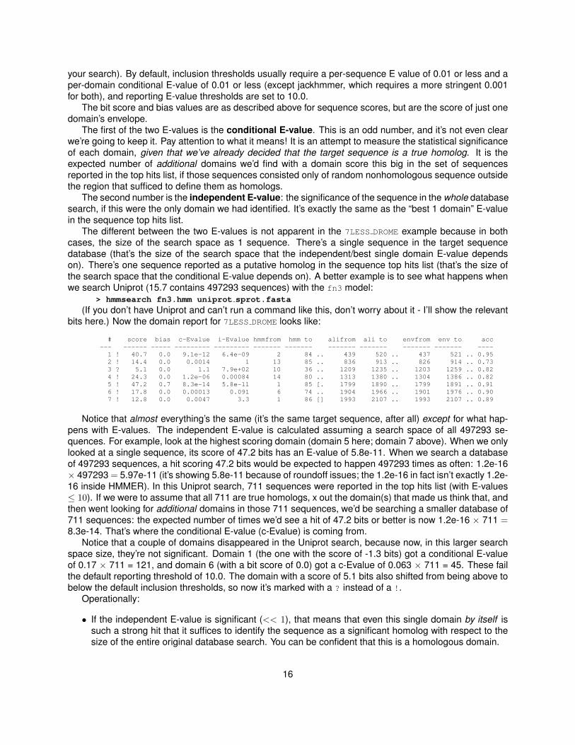
The different between the two E-values is not apparent in the 7LESS DROME example because in bothcases, the size of the search space as 1 sequence. There’s a single sequence in the target sequencedatabase (that’s the size of the search space that the independent/best single domain E-value dependson). There’s one sequence reported as a putative homolog in the sequence top hits list (that’s the size ofthe search space that the conditional E-value depends on). A better example is to see what happens whenwe search Uniprot (15.7 contains 497293 sequences) with the fn3 model:

> hmmsearch fn3.hmm uniprot sprot.fasta(If you don’t have Uniprot and can’t run a command like this, don’t worry about it - I’ll show the relevant

bits here.) Now the domain report for 7LESS DROME looks like:

# score bias c-Evalue i-Evalue hmmfrom hmm to alifrom ali to envfrom env to acc--- ------ ----- --------- --------- ------- ------- ------- ------- ------- ------- ----

1 ! 40.7 0.0 9.1e-12 6.4e-09 2 84 .. 439 520 .. 437 521 .. 0.952 ! 14.4 0.0 0.0014 1 13 85 .. 836 913 .. 826 914 .. 0.733 ? 5.1 0.0 1.1 7.9e+02 10 36 .. 1209 1235 .. 1203 1259 .. 0.824 ! 24.3 0.0 1.2e-06 0.00084 14 80 .. 1313 1380 .. 1304 1386 .. 0.825 ! 47.2 0.7 8.3e-14 5.8e-11 1 85 [. 1799 1890 .. 1799 1891 .. 0.916 ! 17.8 0.0 0.00013 0.091 6 74 .. 1904 1966 .. 1901 1976 .. 0.907 ! 12.8 0.0 0.0047 3.3 1 86 [] 1993 2107 .. 1993 2107 .. 0.89

Notice that almost everything’s the same (it’s the same target sequence, after all) except for what hap-pens with E-values. The independent E-value is calculated assuming a search space of all 497293 se-quences. For example, look at the highest scoring domain (domain 5 here; domain 7 above). When we onlylooked at a single sequence, its score of 47.2 bits has an E-value of 5.8e-11. When we search a databaseof 497293 sequences, a hit scoring 47.2 bits would be expected to happen 497293 times as often: 1.2e-16× 497293 = 5.97e-11 (it’s showing 5.8e-11 because of roundoff issues; the 1.2e-16 in fact isn’t exactly 1.2e-16 inside HMMER). In this Uniprot search, 711 sequences were reported in the top hits list (with E-values≤ 10). If we were to assume that all 711 are true homologs, x out the domain(s) that made us think that, andthen went looking for additional domains in those 711 sequences, we’d be searching a smaller database of711 sequences: the expected number of times we’d see a hit of 47.2 bits or better is now 1.2e-16 × 711 =8.3e-14. That’s where the conditional E-value (c-Evalue) is coming from.

Notice that a couple of domains disappeared in the Uniprot search, because now, in this larger searchspace size, they’re not significant. Domain 1 (the one with the score of -1.3 bits) got a conditional E-valueof 0.17 × 711 = 121, and domain 6 (with a bit score of 0.0) got a c-Evalue of 0.063 × 711 = 45. These failthe default reporting threshold of 10.0. The domain with a score of 5.1 bits also shifted from being above tobelow the default inclusion thresholds, so now it’s marked with a ? instead of a !.

Operationally:

• If the independent E-value is significant (<< 1), that means that even this single domain by itself issuch a strong hit that it suffices to identify the sequence as a significant homolog with respect to thesize of the entire original database search. You can be confident that this is a homologous domain.

16

• Once there’s one or more high-scoring domains in the sequence already, sufficient to decide thatthe sequence contains homologs of your query, you can look (with some caution) at the conditionalE-value to decide the statistical significance of additional weak-scoring domains.

In the Uniprot output, for example, I’d be pretty sure of four of the domains (1, 4, 5, and maybe 6), eachof which has a strong enough independent E-value to declare 7LESS DROME to be an fnIII-domain-containingprotein. Domains 2 and 7 wouldn’t be significant if they were all I saw in the sequence, but once I decidethat 7LESS DROME contains fn3 domains on the basis of the other hits, their conditional E-values indicatethat they are probably also fn3 domains too. Domain 3 is too weak to be sure of, from this search alone, butwould be something to pay attention to.

The next four columns give the endpoints of the reported local alignment with respect to both the querymodel (“hmm from” and “hmm to”) and the target sequence (“ali from” and “ali to”).

It’s not immediately easy to tell from the “to” coordinate whether the alignment ended internally in thequery or target, versus ran all the way (as in a full-length global alignment) to the end(s). To make this morereadily apparent, with each pair of query and target endpoint coordinates, there’s also a little symbology... meaning both ends of the alignment ended internally, and [] means both ends of the alignment werefull-length flush to the ends of the query or target, and [. and .] mean only the left or right end wasflush/full length.

The next two columns (“env from” and “env to”) define the envelope of the domain’s location on thetarget sequence. The envelope is almost always a little wider than what HMMER chooses to show asa reasonably confident alignment. As mentioned earlier, the envelope represents a subsequence thatencompasses most of the posterior probability for a given homologous domain, even if precise endpointsare only fuzzily inferrable. You’ll notice that for higher scoring domains, the coordinates of the envelope andthe inferred alignment will tend to be in tighter agreement, corresponding to sharper posterior probabilitydefining the location of the homologous region.

Operationally, I would use the envelope coordinates to annotate domain locations on target sequences,not the alignment coordinates. However, be aware that when two weaker-scoring domains are close to eachother, envelope coordinates can and will overlap, corresponding to the overlapping uncertainty of where onedomain ends and another begins. In contrast, alignment coordinates generally do not overlap (though thereare cases where even they will overlap3).

The last column is the average posterior probability of the aligned target sequence residues; effectively,the expected accuracy per residue of the alignment.

For comparison, current Uniprot consensus annotation of Sevenless shows seven domains:

FT DOMAIN 311 431 Fibronectin type-III 1.FT DOMAIN 436 528 Fibronectin type-III 2.FT DOMAIN 822 921 Fibronectin type-III 3.FT DOMAIN 1298 1392 Fibronectin type-III 4.FT DOMAIN 1680 1794 Fibronectin type-III 5.FT DOMAIN 1797 1897 Fibronectin type-III 6.FT DOMAIN 1898 1988 Fibronectin type-III 7.

These domains are a pretty tough case to call, actually. HMMER fails to see anything significant over-lapping two of these domains (311-431 and 1680-1794) in the Uniprot search, though it sees a smidgen ofthem when 7LESS DROME alone is the target. HMMER3 sees two new domains (1205-1235 and 1993-2098)that Uniprot currently doesn’t annotate, but these are pretty plausible domains (given that the extracellulardomain of Sevenless is pretty much just a big array of ∼100aa fibronectin repeats.

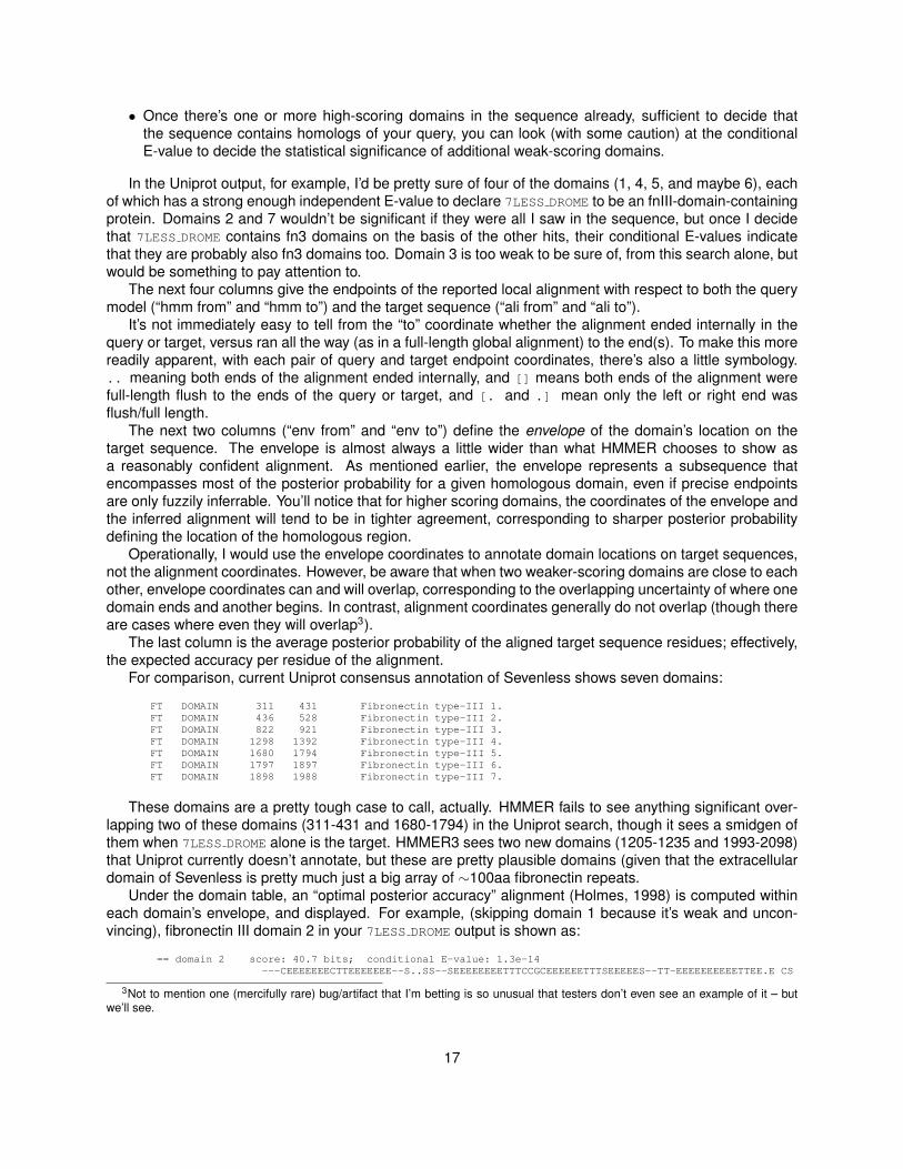
Under the domain table, an “optimal posterior accuracy” alignment (Holmes, 1998) is computed withineach domain’s envelope, and displayed. For example, (skipping domain 1 because it’s weak and uncon-vincing), fibronectin III domain 2 in your 7LESS DROME output is shown as:

== domain 2 score: 40.7 bits; conditional E-value: 1.3e-14---CEEEEEEECTTEEEEEEE--S..SS--SEEEEEEEETTTCCGCEEEEEETTTSEEEEES--TT-EEEEEEEEEETTEE.E CS

3Not to mention one (mercifully rare) bug/artifact that I’m betting is so unusual that testers don’t even see an example of it – butwe’ll see.

17

fn3 2 saPenlsvsevtstsltlsWsppkdgggpitgYeveyqekgegeewqevtvprtttsvtltgLepgteYefrVqavngagegp 84saP ++ + ++ l ++W p + +gpi+gY++++++++++ + e+ vp+ s+ +++L++gt+Y++ + +n++gegp

7LESS_DROME 439 SAPVIEHLMGLDDSHLAVHWHPGRFTNGPIEGYRLRLSSSEGNA-TSEQLVPAGRGSYIFSQLQAGTNYTLALSMINKQGEGP 52078999999999*****************************9998.**********************************9997 PP

The initial header line starts with a == as a little handle for a parsing script to grab hold of. The rest ofthat line, we’ll probably put more information on eventually.

If the model had any consensus structure or reference line annotation that it inherited from your multiplealignment (#=GC SS cons, #=GC RF annotation in Stockholm files), that information is simply regurgitatedas CS or RF annotation lines here. The fn3 model had a consensus structure annotation line.

The line starting with fn3 is the consensus of the query model. Capital letters represent the most con-served (high information content) positions. Dots (.) in this line indicate insertions in the target sequencewith respect to the model.

The midline indicates matches between the query model and target sequence. A + indicates positivescore, which can be interpreted as “conservative substitution”, with respect to what the model expects atthat position.

The line starting with 7LESS DROME is the target sequence. Dashes (-) in this line indicate deletions inthe target sequence with respect to the model.

The bottom line is new to HMMER3. This represents the posterior probability (essentially the expectedaccuracy) of each aligned residue. A 0 means 0-5%, 1 means 5-15%, and so on; 9 means 85-95%, and a *means 95-100% posterior probability. You can use these posterior probabilities to decide which parts of thealignment are well-determined or not. You’ll often observe, for example, that expected alignment accuracydegrades around locations of insertion and deletion, which you’d intuitively expect.

You’ll also see expected alignment accuracy degrade at the ends of an alignment – this is because“alignment accuracy” posterior probabilities currently not only includes whether the residue is aligned toone model position versus others, but also confounded with whether a residue should be considered to behomologous (aligned to the model somewhere) versus not homologous at all.4

These domain table and per-domain alignment reports for each sequence then continue, for each se-quence that was in the per-sequence top hits list.

Finally, at the bottom of the file, you’ll see some summary statistics. For example, at the bottom of theglobins search output, you’ll find something like:

Internal pipeline statistics summary:-------------------------------------Query model(s): 1 (149 nodes)Target sequences: 497293 (175274722 residues)Passed MSV filter: 19416 (0.0390434); expected 9945.9 (0.02)Passed bias filter: 15929 (0.0320314); expected 9945.9 (0.02)Passed Vit filter: 2207 (0.00443803); expected 497.3 (0.001)Passed Fwd filter: 1076 (0.00216371); expected 5.0 (1e-05)Initial search space (Z): 497293 [actual number of targets]Domain search space (domZ): 1075 [number of targets reported over threshold]# CPU time: 7.08u 0.09s 00:00:07.17 Elapsed: 00:00:02.95# Mc/sec: 8852.86//

This gives you some idea of what’s going on in HMMER3’s acceleration pipeline. You’ve got one queryHMM, and the database has 497,293 target sequences. Each sequence goes through a gauntlet of threescoring algorithms called MSV, Viterbi, and Forward, in order of increasing sensitivity and increasing com-putational requirement.

MSV (the “Multi ungapped Segment Viterbi” algorithm) is the new algorithm in HMMER3. It essentiallycalculates the HMM equivalent of BLAST’s sum score – an optimal sum of ungapped high-scoring alignmentsegments. Unlike BLAST, it does this calculation directly, without BLAST’s word hit or hit extension step,using a SIMD vector-parallel algorithm. By default, HMMER3 is configured to allow sequences with a P-value of ≤ 0.02 through the MSV score filter (thus, if the database contained no homologs and P-values

4It may make more sense to condition the posterior probabilities on the assumption that the residue is indeed homologous: giventhat, how likely is it that I’ve got it correctly aligned.

18

were accurately calculated, the highest scoring 2% of the sequences will pass the filter). Here, about 4% ofthe database got through the MSV filter.

A quick check is then done to see if the target sequence is “obviously” so biased in its composition thatit’s unlikely to be a true homolog. This is called the “bias filter”. If you don’t like it (it can occasionally beoveraggressive) you can shut it off with the --nobias option. Here, 15929 sequences pass through the biasfilter.

The Viterbi filter then calculates a gapped optimal alignment score. This is a bit more sensitive than theMSV score, but the Viterbi filter is about four-fold slower than MSV. By default, HMMER3 lets sequenceswith a P-value of ≤ 0.001 through this stage. Here (because there’s a little over a thousand true globinhomologs in this database), much more than that gets through - 2207 sequences.

Then the full Forward score is calculated, which sums over all possible alignments of the profile tothe target sequence. The default allows sequences with a P-value of ≤ 10−5% through; 1076 sequencespassed.

All sequences that make it through the three filters are then subjected to a full probabilistic analysisusing the HMM Forward/Backward algorithms, first to identify domains and assign domain envelopes; thenwithin each individual domain envelope, Forward/Backward calculations are done to determine posteriorprobabilities for each aligned residue, followed by optimal accuracy alignment. The results of this step arewhat you finally see on the output.

Recall the difference between conditional and independent E-values, with their two different searchspace sizes. These search space sizes are reported in the statistics summary.

Finally, it reports the speed of the search in units of Mc/sec (million dynamic programming cells persecond), the CPU time, and the elapsed time. This search took about 2.95 seconds of elapsed (wall clocktime) (running with --cpu 2 on two cores). That’s in the same ballpark as BLAST, depending on whichBLAST you compare to. On the same machine, also running dual-core, NCBI BLAST with one of theseglobin sequences took 3.8 seconds, and WU-BLAST took 7.4 seconds.

Searching a profile HMM database with a query sequence

The hmmscan program is for annotating all the different known/detectable domains in a given sequence.It takes a single query sequence and an HMM database as input. The HMM database might be Pfam,SMART, or TIGRFams, for example, or another collection of your choice.

Step 1: create an HMM database flatfile

An HMM “database” flatfile is simply a concatenation of individual HMM files. To create a database flat-file, you can either build individual HMM files and concatenate them, or you can concatenate Stockholmalignments and use hmmbuild to build an HMM database of all of them in one command.

Let’s create a tiny database called minifam containing models of globin, fn3, and Pkinase (proteinkinase) domains by concatenating model files:

> hmmbuild globins4.hmm tutorial/globins4.sto> hmmbuild fn3.hmm tutorial/fn3.sto> hmmbuild Pkinase.hmm tutorial/Pkinase.sto> cat globins4.hmm fn3.hmm Pkinase.hmm > minifam

We’ll use minifam for our examples in just a bit, but first a few words on other ways to build HMMdatabases, especially big ones. The file tutorials/minifam is the same thing, if you want to just use that.

Alternatively, you can concatenate Stockholm alignment files together (as Pfam does in its big Pfam-A.seed

and Pfam-A.full flatfiles) and use hmmbuild to build HMMs for all the alignments at once. This won’t workproperly for our tutorial alignments, because the globins4.sto alignment doesn’t have an #=GF ID anno-tation line giving a name to the globins4 alignment, so hmmbuild wouldn’t know how to name it correctly. Tobuild a multi-model database from a multi-MSA flatfile, the alignments have to be in Stockholm format (no

19

other MSA format that I’m aware of supports having more than one alignment per file), and each alignmentmust have a name on a #=GF ID line.

But if you happen to have a Pfam seed alignment flatfile Pfam-A.seed around, an example commandwould be:

> hmmbuild Pfam-A.hmm Pfam-A.seedThis would take about two or three hours to build all 10,000 models or so in Pfam. To speed the database

construction process up, hmmbuild supports MPI parallelization.As far as HMMER’s concerned, all you have to do is add --mpi to the command line for hmmbuild,

assuming you’ve compiled support for MPI into it (see the installation instructions). You’ll also need to knowhow to invoke an MPI job in your particular environment, with your job scheduler and MPI distribution. Wecan’t really help you with this – different sites have different cluster environments.

With our scheduler (SGE, the Sun Grid Engine) and our MPI distro (OpenMPI), an example incantationfor building Pfam.hmm from Pfam-A.seed is:

> qsub -N hmmbuild -j y -o errors.out -b y -cwd -V -pe openmpi 128’mpirun -mca btl self,openib,sm -np 128 ./hmmbuild --mpi Pfam.hmm Pfam-A.seed > hmmbuild.out’

This reduces the time to build all of Pfam to about 40 seconds.

Step 2: compress and index the flatfile with hmmpress

The hmmscan program has to read a lot of profile HMMs in a hurry, and HMMER’s ASCII flatfiles are bulky.To accelerate this, hmmscan uses binary compression and indexing of the flatfiles. To use hmmscan, youmust first compress and index your HMM database with the hmmpress program:

> hmmpress minifamThis will quickly produce:

Working... done.Pressed and indexed 3 HMMs (3 names and 2 accessions).Models pressed into binary file: minifam.h3mSSI index for binary model file: minifam.h3iProfiles (MSV part) pressed into: minifam.h3fProfiles (remainder) pressed into: minifam.h3p

and you’ll see these four new binary files in the directory.The tutorial/minifam example has already been pressed, so there are example binary files

tutorial/minifam.h3{m,i,f,p} included in the tutorial.Their format is “proprietary”, which is an open source term of art that means both “I haven’t found time

to document them yet” and “I still might decide to change them arbitrarily without telling you”.

Step 3: search the HMM database with hmmscan

Now we can analyze sequences using our HMM database and hmmscan.For example, the receptor tyrosine kinase 7LESS DROME not only has all those fibronectin type III domains

on its extracellular face, it’s got a protein kinase domain on its intracellular face. Our minifam database hasmodels of both fn3 and Pkinase, as well as the unrelated globins4 model. So what happens when wescan the 7LESS DROME sequence:

> hmmscan minifam tutorial/7LESS DROMEThe header and the first section of the output will look like:

# hmmscan :: search sequence(s) against a profile database# HMMER 3.0b3 (November 2009); http://hmmer.org/# Copyright (C) 2009 Howard Hughes Medical Institute.# Freely distributed under the GNU General Public License (GPLv3).# - - - - - - - - - - - - - - - - - - - - - - - - - - - - - - - - - - - -# query sequence file: 7LESS_DROME# target HMM database: minifam# per-seq hits tabular output: 7LESS.tbl# per-dom hits tabular output: 7LESS.domtbl

20

# - - - - - - - - - - - - - - - - - - - - - - - - - - - - - - - - - - - -

Query: 7LESS_DROME [L=2554]Accession: P13368Description: RecName: Full=Protein sevenless; EC=2.7.10.1;Scores for complete sequence (score includes all domains):

--- full sequence --- --- best 1 domain --- -#dom-E-value score bias E-value score bias exp N Model Description------- ------ ----- ------- ------ ----- ---- -- -------- -----------5.6e-57 178.0 0.4 3.5e-16 47.2 0.7 9.4 9 fn3 Fibronectin type III domain1.1e-43 137.2 0.0 1.7e-43 136.5 0.0 1.3 1 Pkinase Protein kinase domain

The output fields are in the same order and have the same meaning as in hmmsearch’s output.The size of the search space for hmmscan is the number of models in the HMM database (here, 3;

for a Pfam search, on the order of 10000). In hmmsearch, the size of the search space is the number ofsequences in the sequence database. This means that E-values may differ even for the same individualprofile vs. sequence comparison, depending on how you do the search.

For domain, there then follows a domain table and alignment output, just as in hmmsearch. The fn3

annotation, for example, looks like:

Domain and alignment annotation for each model:>> fn3 Fibronectin type III domain

# score bias c-Evalue i-Evalue hmmfrom hmm to alifrom ali to envfrom env to acc--- ------ ----- --------- --------- ------- ------- ------- ------- ------- ------- ----

1 ? -1.3 0.0 0.33 0.5 61 74 .. 396 409 .. 395 411 .. 0.852 ! 40.7 0.0 2.6e-14 3.8e-14 2 84 .. 439 520 .. 437 521 .. 0.953 ! 14.4 0.0 4.1e-06 6.1e-06 13 85 .. 836 913 .. 826 914 .. 0.734 ! 5.1 0.0 0.0032 0.0048 10 36 .. 1209 1235 .. 1203 1259 .. 0.825 ! 24.3 0.0 3.4e-09 5e-09 14 80 .. 1313 1380 .. 1304 1386 .. 0.826 ? 0.0 0.0 0.13 0.19 58 72 .. 1754 1768 .. 1739 1769 .. 0.897 ! 47.2 0.7 2.3e-16 3.5e-16 1 85 [. 1799 1890 .. 1799 1891 .. 0.918 ! 17.8 0.0 3.7e-07 5.5e-07 6 74 .. 1904 1966 .. 1901 1976 .. 0.909 ! 12.8 0.0 1.3e-05 2e-05 1 86 [] 1993 2107 .. 1993 2107 .. 0.89

and an example alignment (of that second domain again):

== domain 2 score: 40.7 bits; conditional E-value: 2.6e-14---CEEEEEEECTTEEEEEEE--S..SS--SEEEEEEEETTTCCGCEEEEEETTTSEEEEES--TT-EEEEEEEEEETTEE.E CS

fn3 2 saPenlsvsevtstsltlsWsppkdgggpitgYeveyqekgegeewqevtvprtttsvtltgLepgteYefrVqavngagegp 84saP ++ + ++ l ++W p + +gpi+gY++++++++++ + e+ vp+ s+ +++L++gt+Y++ + +n++gegp

7LESS_DROME 439 SAPVIEHLMGLDDSHLAVHWHPGRFTNGPIEGYRLRLSSSEGNA-TSEQLVPAGRGSYIFSQLQAGTNYTLALSMINKQGEGP 52078999999999*****************************9998.**********************************9997 PP

You’d think that except for the E-values (which depend on database search space sizes), you should getexactly the same scores, domain number, domain coordinates, and alignment every time you do a searchof the same HMM against the same sequence. And this is actually the case – but in fact, it’s actually notso obvious this should be so, and HMMER is going out of its way to make it so. HMMER uses stochasticsampling algorithms to infer some parameters, and also to infer the exact domain number and domainboundaries in certain difficult cases. If HMMER ran its stochastic samples “properly”, it would see differentsamples every time you ran a program, and all of you would complain to me that HMMER was weird andbuggy because it gave different answers on the same problem. To suppress run-to-run variation, HMMERseeds its random number generator(s) identically every time you do a sequence comparison. If you’re anexpert, and you really want to see the proper stochastic variation that results from any sampling algorithmsthat got run, you can pass a command-line argument of --seed 0 to programs that have this property(hmmbuild and the four search programs).

Creating multiple alignments with hmmalign

The file tutorial/globins45.fa is a FASTA file containing 45 unaligned globin sequences. To align all ofthese to the globins4 model and make a multiple sequence alignment:

> hmmalign globins4.hmm tutorial/globins45.faThe output of this is a Stockholm format multiple alignment file. The first few lines of it look like:

21

# STOCKHOLM 1.0

MYG_ESCGI .-VLSDAEWQLVLNIWAKVEADVAGHGQDILIRLFKGHPETLEKFDKFKH#=GR MYG_ESCGI PP ..69**********************************************MYG_HORSE g--LSDGEWQQVLNVWGKVEADIAGHGQEVLIRLFTGHPETLEKFDKFKH#=GR MYG_HORSE PP 8..89*********************************************MYG_PROGU g--LSDGEWQLVLNVWGKVEGDLSGHGQEVLIRLFKGHPETLEKFDKFKH#=GR MYG_PROGU PP 8..89*********************************************MYG_SAISC g--LSDGEWQLVLNIWGKVEADIPSHGQEVLISLFKGHPETLEKFDKFKH#=GR MYG_SAISC PP 8..89*********************************************MYG_LYCPI g--LSDGEWQIVLNIWGKVETDLAGHGQEVLIRLFKNHPETLDKFDKFKH#=GR MYG_LYCPI PP 8..89*********************************************MYG_MOUSE g--LSDGEWQLVLNVWGKVEADLAGHGQEVLIGLFKTHPETLDKFDKFKN#=GR MYG_MOUSE PP 8..89*********************************************MYG_MUSAN v------DWEKVNSVWSAVESDLTAIGQNILLRLFEQYPESQNHFPKFKN...

and so on.Notice those PP annotation lines. That’s posterior probability annotation, as in the single sequence

alignments that hmmscan and hmmsearch showed. This essentially represents the confidence that eachresidue is aligned where it should be.

hmmalign currently has a “feature” that we’re aware of. Recall that HMMER3 only does local alignments.Here, we know that we’ve provided full length globin sequences, and globins4 is a full length globin model.We’d probably like hmmalign to produce a global alignment. It can’t currently do that. If it doesn’t quitemanage to extend its local alignment to the full length of a target globin sequence, you’ll get a weird-lookingeffect, as the nonmatching termini are pulled out to the left or right. For example, look at the N-terminal gin MYG HORSE above. H3 is about 80% confident that this residue is nonhomologous, though any sensibleperson would align it into the first globin consensus column.

Look at the end of that first block of Stockholm alignment, where you’ll see:

...HBBL_RANCA v-HWTAEEKAVINSVWQKV--DVEQDGHEALTRLFIVYPWTQRYFSTFGD#=GR HBBL_RANCA PP 6.6799*************..*****************************HBB2_TRICR .VHLTAEDRKEIAAILGKV--NVDSLGGQCLARLIVVNPWSRRYFHDFGD#=GR HBB2_TRICR PP .69****************..*****************************#=GC PP_cons .679**********************************************#=GC RF .xxxxxxxxxxxxxxxxxxxxxxxxxxxxxxxxxxxxxxxxxxxxxxxxx

The #=GC PP cons line is Stockholm-format consensus posterior probability annotation for the entirecolumn. It’s calculated simply as the arithmetic mean of the per-residue posterior probabilities in that col-umn. This should prove useful in phylogenetic inference applications, for example, where it’s common tomask away nonconfidently aligned columns of a multiple alignment. The PP cons line provides an objectivemeasure of the confidence assigned to each column.

The #=GC RF line is Stockholm-format reference coordinate annotation, with an x marking each columnthat the profile considered to be consensus.

Single sequence queries using phmmer

The phmmer program is for searching a single sequence query against a sequence database, much asBLASTP or FASTA would do. phmmer works essentially just like hmmsearch does, except you provide a querysequence instead of a query profile HMM.

Internally, HMMER builds a profile HMM from your single query sequence, using a simple position-independent scoring system (BLOSUM62 scores converted to probabilities, plus a gap-open and gap-extend probability).

The file tutorial/HBB HUMAN is a FASTA file containing the human β−globin sequence as an examplequery. If you have a sequence database such as uniprot sprot.fasta, make that your target database;otherwise, use tutorial/globins45.fa as a small example:

> phmmer tutorial/HBB HUMAN uniprot sprot.faor

> phmmer tutorial/HBB HUMAN tutorial/globins45.fa

22

Everything about the output is essentially as previously described for hmmsearch.

Iterative searches using jackhmmer

The jackhmmer program is for searching a single sequence query iteratively against a sequence database,much as PSI-BLAST would do.

The first round is identical to a phmmer search. All the matches that pass the inclusion thresholds areput in a multiple alignment. In the second (and subsequent) rounds, a profile is made from these results,and the database is searched again with the profile.

Iterations continue either until no new sequences are detected or the maximum number of iterations isreached. By default, the maximum number of iterations is 5; you can change this with the -N option.

Your original query sequence is always included in the multiple alignments, whether or not it appears inthe database.5 The “consensus” columns assigned to each multiple alignment always correspond exactly tothe residues of your query, so the coordinate system of every profile is always the same as the numberingof residues in your query sequence, 1..L for a sequence of length L.

Assuming you have Uniprot or something like it handy, here’s an example command line for a jackhmmersearch:

> jackhmmer tutorial/HBB HUMAN uniprot sprot.fa

One difference from phmmer output you’ll notice is that jackhmmer marks “new” sequences with a +

and “lost” sequences with a -. New sequences are sequences that pass the inclusion threshold(s) inthis round, but didn’t in the round before. Lost sequences are the opposite: sequences that passed theinclusion threshold(s) in the previous round, but have now fallen beneath (yet are still in the reported hits –it’s possible, though rare, to lose sequences utterly, if they no longer even pass the reporting threshold(s)).In the first round, everything above the inclusion thresholds is marked with a +, and nothing is marked witha -. For example, the top of this output looks like:

# jackhmmer :: iteratively search a protein sequence against a protein database# HMMER 3.0b3 (November 2009); http://hmmer.org/# Copyright (C) 2009 Howard Hughes Medical Institute.# Freely distributed under the GNU General Public License (GPLv3).# - - - - - - - - - - - - - - - - - - - - - - - - - - - - - - - - - - - -# query sequence file: HBB_HUMAN# target sequence database: uniprot_sprot.fasta# per-seq hits tabular output: hbb-jack.tbl# per-dom hits tabular output: hbb-jack.domtbl# - - - - - - - - - - - - - - - - - - - - - - - - - - - - - - - - - - - -

Query: HBB_HUMAN [L=146]Description: Human beta hemoglobin.

Scores for complete sequences (score includes all domains):--- full sequence --- --- best 1 domain --- -#dom-E-value score bias E-value score bias exp N Sequence Description------- ------ ----- ------- ------ ----- ---- -- -------- -----------

+ 2.3e-98 331.4 0.0 2.5e-98 331.2 0.0 1.0 1 sp|P68871|HBB_HUMAN Hemoglobin subunit beta OS=Homo sapien+ 2.3e-98 331.4 0.0 2.5e-98 331.2 0.0 1.0 1 sp|P68872|HBB_PANPA Hemoglobin subunit beta OS=Pan paniscu+ 2.3e-98 331.4 0.0 2.5e-98 331.2 0.0 1.0 1 sp|P68873|HBB_PANTR Hemoglobin subunit beta OS=Pan troglod+ 9.1e-98 329.4 0.0 1e-97 329.3 0.0 1.0 1 sp|P02024|HBB_GORGO Hemoglobin subunit beta OS=Gorilla gor+ 2e-96 325.1 0.0 2.2e-96 324.9 0.0 1.0 1 sp|P02025|HBB_HYLLA Hemoglobin subunit beta OS=Hylobates l+ 2e-95 321.8 0.0 2.2e-95 321.7 0.0 1.0 1 sp|P02032|HBB_SEMEN Hemoglobin subunit beta OS=Semnopithec...

That continues until the inclusion threshold is reached, at which point you see a tagline “inclusion thresh-old” indicating where the threshold was set:

+ 0.00076 24.1 0.0 0.00083 24.0 0.0 1.0 1 sp|P02180|MYG_BALPH Myoglobin OS=Balaenoptera physalus GN=+ 0.00087 23.9 0.0 0.0009 23.9 0.0 1.0 1 sp|P02148|MYG_PONPY Myoglobin OS=Pongo pygmaeus GN=MB PE=1

5If it is in the database, it will almost certainly be included in the internal multiple alignment twice, once because it’s the queryand once because it’s a significant database match to itself. This redundancy won’t screw up the alignment, because sequences aredownweighted for redundancy anyway.

23

------ inclusion threshold ------0.0013 23.3 0.3 0.021 19.4 0.2 2.1 1 sp|P81044|HBAZ_MACEU Hemoglobin subunit zeta (Fragments) OS0.0021 22.7 0.0 0.0022 22.6 0.0 1.0 1 sp|P02182|MYG_ZIPCA Myoglobin OS=Ziphius cavirostris GN=MB

The domain output and search statistics are then shown just as in phmmer. At the end of this firstiteration, you’ll see some output that starts with @@ (this is a simple tag that lets you search through the fileto find the end of one iteration and the beginning of another):

@@ New targets included: 894@@ New alignment includes: 895 subseqs (was 1), including original query@@ Continuing to next round.

@@@@ Round: 2@@ Included in MSA: 895 subsequences (query + 894 subseqs from 894 targets)@@ Model size: 146 positions@@

This (obviously) is telling you that the new alignment contains 895 sequences, your query plus 894significant matches. For round two, it’s built a new model from this alignment. Now for round two, it fires offwhat’s essentially an hmmsearch of the target database with this new model:

Scores for complete sequences (score includes all domains):--- full sequence --- --- best 1 domain --- -#dom-E-value score bias E-value score bias exp N Sequence Description------- ------ ----- ------- ------ ----- ---- -- -------- -----------1.5e-67 231.0 0.2 1.7e-67 230.8 0.1 1.0 1 sp|P02055|HBB_MELME Hemoglobin subunit beta OS=Meles meles2.3e-67 230.4 0.4 2.6e-67 230.2 0.3 1.0 1 sp|P81042|HBE_MACEU Hemoglobin subunit epsilon OS=Macropus2.7e-67 230.2 0.3 2.9e-67 230.0 0.2 1.0 1 sp|P15449|HBB_MELCA Hemoglobin subunit beta OS=Mellivora c3.3e-67 229.9 0.2 3.7e-67 229.7 0.2 1.0 1 sp|P68046|HBB_ODORO Hemoglobin subunit beta OS=Odobenus ro

...

If you skim down through this output, you’ll start seeing newly included sequences marked with +’s, suchas:

...9.8e-30 108.3 0.0 1.1e-29 108.2 0.0 1.0 1 sp|P87497|MYG_CHIRA Myoglobin OS=Chionodraco rastrospinosu

+ 1.4e-29 107.8 0.3 1.5e-29 107.7 0.2 1.0 1 sp|P14399|MYG_MUSAN Myoglobin OS=Mustelus antarcticus GN=m1.5e-29 107.7 0.3 2e-29 107.3 0.2 1.0 1 sp|P80017|GLBD_CAUAR Globin D, coelomic OS=Caudina arenicol

3e-29 106.8 0.0 3.3e-29 106.6 0.0 1.0 1 sp|P02022|HBAM_RANCA Hemoglobin heart muscle subunit alpha-4e-29 106.3 0.0 4.4e-29 106.2 0.0 1.0 1 sp|Q9DEP0|MYG_CRYAN Myoglobin OS=Cryodraco antarcticus GN=

+ 9.3e-29 105.2 0.2 1e-28 105.0 0.1 1.0 1 sp|P14397|MYG_GALGA Myoglobin OS=Galeorhinus galeus GN=mb1.3e-28 104.7 0.0 1.6e-28 104.4 0.0 1.0 1 sp|P0C227|GLB_NERAL Globin OS=Nerita albicilla PE=1 SV=1

2e-28 104.1 0.0 2.4e-28 103.8 0.0 1.0 1 sp|P09106|HBAT_PAPAN Hemoglobin subunit theta-1 OS=Papio an+ 2.8e-28 103.6 0.1 3.1e-28 103.5 0.1 1.0 1 sp|P14398|MYG_GALJA Myoglobin OS=Galeorhinus japonicus GN=

7.9e-26 95.7 0.0 8.8e-26 95.5 0.0 1.0 1 sp|P23216|GLBP1_GLYDI Globin, major polymeric component P1 O...

It’s unusual to see sequences get lost (and marked with -), but it can happen; it doesn’t happen in thisglobin example.

After round 2, many more globin sequences have been found:@@ New targets included: 167@@ New alignment includes: 1064 subseqs (was 895), including original query@@ Continuing to next round.

@@@@ Round: 3@@ Included in MSA: 1064 subsequences (query + 1063 subseqs from 1061 targets)@@ Model size: 146 positions@@

Because new sequences were included, it keeps going to round three, and then again to round four, thenagain to round five. After round five (where this example has found 1113 included hits in the database), thesearch ends quietly because there’s a default maximum of five iterations, and you get:

@@ New targets included: 1@@ New alignment includes: 1114 subseqs (was 1113), including original query//

That // marks the end of the results for one query.

24

4 File formats

HMMER profile HMM files

The file tutorial/fn3.hmm gives an example of a HMMER3 ASCII save file. An abridged version is shownhere, where (. . . ) mark deletions made for clarity and space:

HMMER3/b [3.0b2 | June 2009]NAME fn3ACC PF00041.12DESC Fibronectin type III domainLENG 86ALPH aminoRF noCS yesMAP yesDATE Mon Jun 15 09:39:41 2009NSEQ 106EFFN 11.415833CKSUM 72638555GA 8.00 7.20TC 8.00 7.20NC 7.90 7.90STATS LOCAL MSV -9.4043 0.71847STATS LOCAL VITERBI -9.7737 0.71847STATS LOCAL FORWARD -3.8341 0.71847HMM A C D E F G H I (...) Y

m->m m->i m->d i->m i->i d->m d->dCOMPO 2.70271 4.89246 3.02314 2.64362 3.59817 2.82566 3.74147 3.08574 (...) 3.22607

2.68618 4.42225 2.77519 2.73123 3.46354 2.40513 3.72494 3.29354 (...) 3.615030.00338 6.08833 6.81068 0.61958 0.77255 0.00000 *

1 3.16986 5.21447 4.52134 3.29953 4.34285 4.18764 4.30886 3.35801 (...) 3.93889 1 - -2.68629 4.42236 2.77530 2.73088 3.46365 2.40512 3.72505 3.29365 (...) 3.615140.09796 2.38361 6.81068 0.10064 2.34607 0.48576 0.95510

2 2.70230 5.97353 2.24744 2.62947 5.31433 2.60356 4.43584 4.79731 (...) 4.25623 3 - -2.68618 4.42225 2.77519 2.73123 3.46354 2.40513 3.72494 3.29354 (...) 3.615030.00338 6.08833 6.81068 0.61958 0.77255 0.48576 0.95510

(...)85 2.48488 5.72055 3.87501 1.97538 3.04853 3.48010 4.51877 3.51898 (...) 3.43366 120 - B

2.68618 4.42225 2.77519 2.73123 3.46354 2.40513 3.72494 3.29354 (...) 3.615030.00338 6.08833 6.81068 0.61958 0.77255 0.48576 0.95510

86 3.03720 5.94099 3.75455 2.96917 5.26587 2.91682 3.66571 4.11840 (...) 4.99111 121 - E2.68618 4.42225 2.77519 2.73123 3.46354 2.40513 3.72494 3.29354 (...) 3.615030.00227 6.08723 * 0.61958 0.77255 0.00000 *

//

An HMM file consists of one or more HMMs. Each HMM starts with the identifier HMMER3/b and endswith // on a line by itself. The identifier allows backward compatibility as the HMMER software evolves: ittells the parser this file is from HMMER3’s save file format version b. (The 3/a format was used in alpha testversions of HMMER3.) The closing // allows multiple HMMs to be concatenated.

The format is divided into two regions. The first region contains textual information and miscalleneousparameters in a roughly tag-value scheme. This section ends with a line beginning with the keyword HMM.The second region is a tabular, whitespace-limited format for the main model parameters.

All probability parameters are all stored as negative natural log probabilities with five digits of precision tothe right of the decimal point, rounded. For example, a probability of 0.25 is stored as − log 0.25 = 1.38629.The special case of a zero probability is stored as ’*’.

Spacing is arranged for human readability, but the parser only cares that fields are separated by at leastone space character.

A more detailed description of the format follows.

header section

The header section is parsed line by line in a tag/value format. Each line type is either mandatory oroptional as indicated.

HMMER3/b Unique identifier for the save file format version; the /b means that this is HMMER3HMM file format version b. When HMMER3 changes its save file format, the revi-sion code advances. This way, parsers may easily remain backwards compatible.The remainder of the line after the HMMER3/b tag is free text that is ignored by theparser. HMMER currently writes its version number and release date in bracketshere, e.g. [3.0b2 | June 2009] in this example. Mandatory.

25

NAME <s> Model name; <s> is a single word containing no spaces or tabs. The name isnormally picked up from the #=GF ID line from a Stockholm alignment file. Ifthis is not present, the name is created from the name of the alignment file byremoving any file type suffix. For example, an otherwise nameless HMM built fromthe alignment file rrm.slx would be named rrm. Mandatory.

ACC <s> Accession number; <s> is a one-word accession number. This is picked up fromthe #=GF AC line in a Stockholm format alignment. Optional.

DESC <s> Description line; <s> is a one-line free text description. This is picked up from the#=GF DE line in a Stockholm alignment file. Optional.

LENG <d> Model length; <d>, a positive nonzero integer, is the number of match states in themodel. Mandatory.

ALPH <s> Symbol alphabet type. For biosequence analysis models, <s> is amino, DNA, orRNA (case insensitive). There are also other accepted alphabets for purposes be-yond biosequence analysis, including coins, dice, and custom. This determinesthe symbol alphabet and the size of the symbol emission probability distributions.If amino, the alphabet size K is set to 20 and the symbol alphabet to “ACDE-FGHIKLMNPQRSTVWY” (alphabetic order); if DNA, the alphabet size K is set to 4and the symbol alphabet to “ACGT”; if RNA, the alphabet size K is set to 4 and thesymbol alphabet to “ACGU”. Mandatory.

RF <s> Reference annotation flag; <s> is either no or yes (case insensitive). If yes, thereference annotation character field for each match state in the main model (seebelow) is valid; if no, these characters are ignored. Reference column annotationis picked up from a Stockholm alignment file’s #=GC RF line. It is propagated toalignment outputs, and also may optionally be used to define consensus matchcolumns in profile HMM construction. Optional; assumed to be no if not present.

CS <s> Consensus structure annotation flag; <s> is either no or yes (case insensitive). Ifyes, the consensus structure character field for each match state in the main model(see below) is valid; if no these characters are ignored. Consensus structure an-notation is picked up from a Stockholm file’s #=GC SS_cons line, and propagatedto alignment displays. Optional; assumed to be no if not present.

MAP <s> Map annotation flag; <s> is either no or yes (case insensitive). If set to yes, themap annotation field in the main model (see below) is valid; if no, that field will beignored. The HMM/alignment map annotates each match state with the index ofthe alignment column from which it came. It can be used for quickly mapping anysubsequent HMM alignment back to the original multiple alignment, via the model.Optional; assumed to be no if not present.

DATE <s> Date the model was constructed; <s> is a free text date string. This field is onlyused for logging purposes.1 Optional.

COM [<n>] <s> Command line log; <n> counts command line numbers, and <s> is a one-line com-mand. There may be more than one COM line per save file, each numbered startingfrom n = 1. These lines record every HMMER command that modified the savefile. This helps us reproducibly and automatically log how Pfam models have beenconstructed, for example. Optional.

1HMMER does not use dates for any purpose other than human-readable annotation, so it is no more prone than you are to Y2K,Y2038, or any other date-related eschatology.

26

NSEQ <d> Sequence number; <d> is a nonzero positive integer, the number of sequences thatthe HMM was trained on. This field is only used for logging purposes. Optional.

EFFN <f> Effective sequence number; <f> is a nonzero positive real, the effective total num-ber of sequences determined by hmmbuild during sequence weighting, for combin-ing observed counts with Dirichlet prior information in parameterizing the model.This field is only used for logging purposes. Optional.

CKSUM <d> Training alignment checksum; <d> is a nonnegative unsigned 32-bit integer. Thisnumber is calculated from the training sequence data, and used in conjunctionwith the alignment map information to verify that a given alignment is indeed thealignment that the map is for. Optional.

GA <f> <f> Pfam gathering thresholds GA1 and GA2. See Pfam documentation of GA lines.Optional.

TC <f> <f> Pfam trusted cutoffs TC1 and TC2. See Pfam documentation of TC lines. Op-tional.

NC <f> <f> Pfam noise cutoffs NC1 and NC2. See Pfam documentation of NC lines. Optional.

STATS <s1> <s2> <f1> <f2> Statistical parameters needed for E-value calculations. <s1> is the model’salignment mode configuration: currently only LOCAL is recognized. <s2> is thename of the score distribution: currently MSV, VITERBI, and FORWARD are recog-nized. <f1> and <f2> are two real-valued parameters controlling location and slopeof each distribution, respectively; µ and λ for Gumbel distributions for MSV andViterbi scores, and τ and λ for exponential tails for Forward scores. λ values mustbe positive. All three lines or none of them must be present: when all three arepresent, the model is considered to be calibrated for E-value statistics. Optional.

HMM Flags the start of the main model section. Solely for human readability of thetabular model data, the symbol alphabet is shown on the HMM line, aligned to thefields of the match and insert symbol emission distributions in the main modelbelow. The next line is also for human readability, providing column headers forthe state transition probability fields in the main model section that follows. Thoughunparsed after the HMM tag, the presence of two header lines is mandatory: theparser always skips the line after the HMM tag line.

COMPO <f>*K The first line in the main model section may be an optional line starting with COMPO:these are the model’s overall average match state emission probabilities, which areused as a background residue composition in the “filter null” model. The K fieldson this line are log probabilities for each residue in the appropriate biosequencealphabet’s order. Optional.

main model section

All the remaining fields are mandatory.The first two lines in the main model section are atypical.2 They contain information for the core model’s

BEGIN node. This is stored as model node 0, and match state 0 is treated as the BEGIN state. The beginstate is mute, so there are no match emission probabilities. The first line is the insert 0 emissions. Thesecond line contains the transitions from the begin state and insert state 0. These seven numbers are:

2That is, the first two lines after the optional COMPO line. Don’t be confused by the presence of an optional COMPO line here. TheCOMPO line is placed in the model section, below the residue column headers, because it’s an array of numbers much like residuescores, but it’s not really part of the model.

27

B → M1, B → I0, B → D1; I0 → M1, I0 → I0; then a 0.0 and a ’*’, because by convention, nonexistenttransitions from the nonexistent delete state 0 are set to log 1 = 0 and log 0 = −∞ = ‘*’.

The remainder of the model has three lines per node, for M nodes (where M is the number of matchstates, as given by the LENG line). These three lines are (K is the alphabet size in residues):

Match emission line The first field is the node number (1 . . .M ). The parser verifies this number as aconsistency check (it expects the nodes to come in order). The next K numbers formatch emissions, one per symbol, in alphabetic order.

The next field is the MAP annotation for this node. If MAP was yes in the header,then this is an integer, representing the alignment column index for this match state(1..alen); otherwise, this field is ‘-’.

The next field is the RF annotation for this node. If RF was yes in the header, thenthis is a single character, representing the reference annotation for this match state;otherwise, this field is ‘-’.

The next field is the CS annotation for this node. If CS was yes, then this is a singlecharacter, representing the consensus structure at this match state; otherwise thisfield is ‘-’.

Insert emission line The K fields on this line are the insert emission scores, one per symbol, in alphabeticorder.

State transition line The seven fields on this line are the transitions for node k, in the order shown by thetransition header line: Mk →Mk+1, Ik, Dk+1; Ik →Mk+1, Ik; Dk →Mk+1, Dk+1.

For transitions from the final node M , match state M + 1 is interpreted as the ENDstate E, and there is no delete state M + 1; therefore the final Mk → Dk+1 andDk → Dk+1 transitions are always * (zero probability), and the final Dk → Mk+1

transition is always 0.0 (probability 1.0).

Finally, the last line of the format is the “//” record separator.

Stockholm, the recommended multiple sequence alignment format

The Pfam and Rfam Consortiums have developed a multiple sequence alignment format called “Stockholmformat” that allows rich and extensible annotation.

Most popular multiple alignment file formats can be changed into a minimal Stockholm format file just byadding a Stockholm header line and a trailing // terminator:

# STOCKHOLM 1.0

seq1 ACDEF...GHIKLseq2 ACDEF...GHIKLseq3 ...EFMNRGHIKL

seq1 MNPQTVWYseq2 MNPQTVWYseq3 MNPQT...//

The first line in the file must be # STOCKHOLM 1.x, where x is a minor version number for the formatspecification (and which currently has no effect on my parsers). This line allows a parser to instantly identifythe file format.

In the alignment, each line contains a name, followed by the aligned sequence. A dash, period, un-derscore, or tilde (but not whitespace) denotes a gap. If the alignment is too long to fit on one line, thealignment may be split into multiple blocks, with blocks separated by blank lines. The number of sequences,their order, and their names must be the same in every block. Within a given block, each (sub)sequence

28

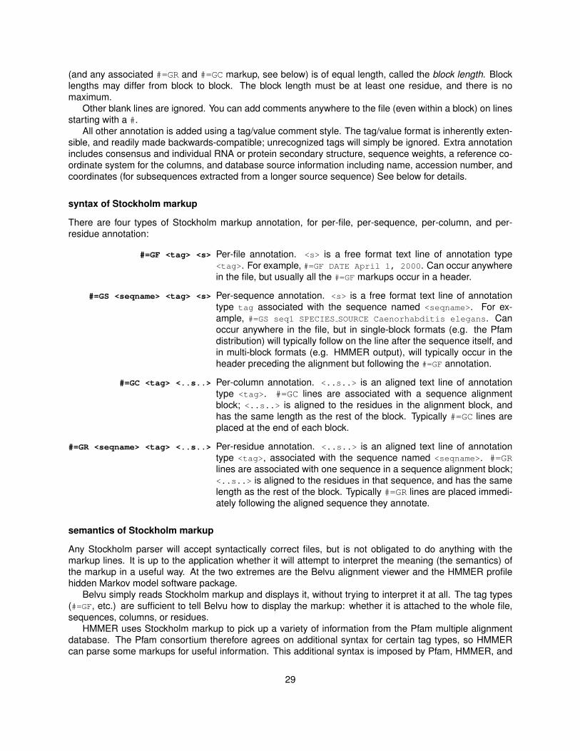
(and any associated #=GR and #=GC markup, see below) is of equal length, called the block length. Blocklengths may differ from block to block. The block length must be at least one residue, and there is nomaximum.

Other blank lines are ignored. You can add comments anywhere to the file (even within a block) on linesstarting with a #.

All other annotation is added using a tag/value comment style. The tag/value format is inherently exten-sible, and readily made backwards-compatible; unrecognized tags will simply be ignored. Extra annotationincludes consensus and individual RNA or protein secondary structure, sequence weights, a reference co-ordinate system for the columns, and database source information including name, accession number, andcoordinates (for subsequences extracted from a longer source sequence) See below for details.

syntax of Stockholm markup

There are four types of Stockholm markup annotation, for per-file, per-sequence, per-column, and per-residue annotation:

#=GF <tag> <s> Per-file annotation. <s> is a free format text line of annotation type<tag>. For example, #=GF DATE April 1, 2000. Can occur anywherein the file, but usually all the #=GF markups occur in a header.

#=GS <seqname> <tag> <s> Per-sequence annotation. <s> is a free format text line of annotationtype tag associated with the sequence named <seqname>. For ex-ample, #=GS seq1 SPECIES SOURCE Caenorhabditis elegans. Canoccur anywhere in the file, but in single-block formats (e.g. the Pfamdistribution) will typically follow on the line after the sequence itself, andin multi-block formats (e.g. HMMER output), will typically occur in theheader preceding the alignment but following the #=GF annotation.

#=GC <tag> <..s..> Per-column annotation. <..s..> is an aligned text line of annotationtype <tag>. #=GC lines are associated with a sequence alignmentblock; <..s..> is aligned to the residues in the alignment block, andhas the same length as the rest of the block. Typically #=GC lines areplaced at the end of each block.

#=GR <seqname> <tag> <..s..> Per-residue annotation. <..s..> is an aligned text line of annotationtype <tag>, associated with the sequence named <seqname>. #=GRlines are associated with one sequence in a sequence alignment block;<..s..> is aligned to the residues in that sequence, and has the samelength as the rest of the block. Typically #=GR lines are placed immedi-ately following the aligned sequence they annotate.

semantics of Stockholm markup

Any Stockholm parser will accept syntactically correct files, but is not obligated to do anything with themarkup lines. It is up to the application whether it will attempt to interpret the meaning (the semantics) ofthe markup in a useful way. At the two extremes are the Belvu alignment viewer and the HMMER profilehidden Markov model software package.

Belvu simply reads Stockholm markup and displays it, without trying to interpret it at all. The tag types(#=GF, etc.) are sufficient to tell Belvu how to display the markup: whether it is attached to the whole file,sequences, columns, or residues.

HMMER uses Stockholm markup to pick up a variety of information from the Pfam multiple alignmentdatabase. The Pfam consortium therefore agrees on additional syntax for certain tag types, so HMMERcan parse some markups for useful information. This additional syntax is imposed by Pfam, HMMER, and

29

other software of mine, not by Stockholm format per se. You can think of Stockholm as akin to XML, andwhat my software reads as akin to an XML DTD, if you’re into that sort of structured data format lingo.

The Stockholm markup tags that are parsed semantically by my software are as follows:

recognized #=GF annotations

ID <s> Identifier. <s> is a name for the alignment; e.g. “rrm”. One word. Unique in file.

AC <s> Accession. <s> is a unique accession number for the alignment; e.g. “PF00001”. Used by thePfam database, for instance. Often a alphabetical prefix indicating the database (e.g. “PF”)followed by a unique numerical accession. One word. Unique in file.

DE <s> Description. <s> is a free format line giving a description of the alignment; e.g. “RNA recogni-tion motif proteins”. One line. Unique in file.

AU <s> Author. <s> is a free format line listing the authors responsible for an alignment; e.g. “BatemanA”. One line. Unique in file.

GA <f> <f> Gathering thresholds. Two real numbers giving HMMER bit score per-sequence and per-domain cutoffs used in gathering the members of Pfam full alignments.

NC <f> <f> Noise cutoffs. Two real numbers giving HMMER bit score per-sequence and per-domaincutoffs, set according to the highest scores seen for unrelated sequences when gatheringmembers of Pfam full alignments.

TC <f> <f> Trusted cutoffs. Two real numbers giving HMMER bit score per-sequence and per-domaincutoffs, set according to the lowest scores seen for true homologous sequences that wereabove the GA gathering thresholds, when gathering members of Pfam full alignments.

recognized #=GS annotations

WT <f> Weight. <f> is a positive real number giving the relative weight for a sequence, usually used tocompensate for biased representation by downweighting similar sequences. Usually the weightsaverage 1.0 (e.g. the weights sum to the number of sequences in the alignment) but this is notrequired. Either every sequence must have a weight annotated, or none of them can.

AC <s> Accession. <s> is a database accession number for this sequence. (Compare the #=GF AC markup,which gives an accession for the whole alignment.) One word.

DE <s> Description. <s> is one line giving a description for this sequence. (Compare the #=GF DE markup,which gives a description for the whole alignment.)

recognized #=GC annotations

RF Reference line. Any character is accepted as a markup for a column. The intent is to allow labelingthe columns with some sort of mark.

SS cons Secondary structure consensus. For protein alignments, DSSP codes or gaps are accepted asmarkup: [HGIEBTSCX.- ], where H is alpha helix, G is 3/10-helix, I is p-helix, E is extended strand,B is a residue in an isolated b-bridge, T is a turn, S is a bend, C is a random coil or loop, and X isunknown (for instance, a residue that was not resolved in a crystal structure).

SA cons Surface accessibility consensus. 0-9, gap symbols, or X are accepted as markup. 0 means<10% accessible residue surface area, 1 means <20%, 9 means <100%, etc. X means unknownstructure.

30

recognized #=GR annotations

SS Secondary structure consensus. See #=GC SS cons above.

SA Surface accessibility consensus. See #=GC SA cons above.

PP Posterior probability for an aligned residue. This represents the probability that this residue is assignedto the HMM state corresponding to this alignment column, as opposed to some other state. (Notethat a residue can be confidently unaligned : a residue in an insert state or flanking N or C state mayhave high posterior probability.) The posterior probability is encoded as 11 possible characters 0-9*:0.0 ≤ p < 0.05 is coded as 0, 0.05 ≤ p < 0.15 is coded as 1, (... and so on ...), 0.85 ≤ p < 0.95 is codedas 9, and 0.95 ≤ p ≤ 1.0 is coded as ’*’. Gap characters appear in the PP line where no residue hasbeen assigned.

31

References

Altschul, S. F., Madden, T. L., Schaffer, A. A., Zhang, J., Zhang, Z., Miller, W., and Lipman, D. J. (1997).Gapped BLAST and PSI-BLAST: A new generation of protein database search programs. Nucl. AcidsRes., 25:3389–3402.

Bashford, D., Chothia, C., and Lesk, A. M. (1987). Determinants of a protein fold: Unique features of theglobin amino acid sequences. J. Mol. Biol., 196:199–216.

Durbin, R., Eddy, S. R., Krogh, A., and Mitchison, G. J. (1998). Biological Sequence Analysis: ProbabilisticModels of Proteins and Nucleic Acids. Cambridge University Press, Cambridge UK.

Eddy, S. R. (1998). Profile hidden Markov models. Bioinformatics, 14:755–763.

Eddy, S. R. (2008). A probabilistic model of local sequence alignment that simplifies statistical significanceestimation. PLoS Comput. Biol., 4:e1000069.

Holmes, I. (1998). Studies in Probabilistic Sequence Alignment and Evolution. PhD thesis, University ofCambridge.

Karlin, S. and Altschul, S. F. (1990). Methods for assessing the statistical significance of molecular sequencefeatures by using general scoring schemes. Proc. Natl. Acad. Sci. USA, 87:2264–2268.

Karlin, S. and Altschul, S. F. (1993). Applications and statistics for multiple high-scoring segments in molec-ular sequences. Proc. Natl. Acad. Sci. USA, 90:5873–5877.

Krogh, A., Brown, M., Mian, I. S., Sjolander, K., and Haussler, D. (1994). Hidden Markov models in compu-tational biology: Applications to protein modeling. J. Mol. Biol., 235:1501–1531.

32