1

BUSINESS CYCLES

Introduction

We now turn to the study of the macroeconomy in the short run. In contrast to our study thus

far where we were analysing the data over periods of 10 years in length, we will be looking at

the data over much shorter periods of time of a year or less. Indeed, for the purpose of the

short-run, the preferred frequency of data is at the quarterly level.

The main objective of this chapter is to describe the ways by which the profession has gone

about documenting the properties of an economy over the short-run, and summarizing the

properties. There is no single way of doing this. In fact, there are two dominant approaches

in use for documenting the business cycle properties. The first has a much longer history and

goes under the heading of Business Cycle dating. The other is fairly new and goes under the

heading of Business Cycle Regularities.

Business Cycle Dating

Business Cycle dating has a long history in economics. It is based on the pioneer work of the

American economist, Wesley C. Mitchell (1913, 1922). Although these early works

introduced Mitchell’s idea of the business cycle being a recurring phenomenon with four

distinct phases, his clearest definition appears in a work with Arthur burns in 1946. On page

3, Burns and Mitchell define the business cycle as

…a cycle consist of expansion occurring at about the same tin in many economic

activities, followed by similarly general recession, contractions, and revivals which

merge into the expansion phase of the next cycle; this sequence of changes is recurrent

2

but not periodic; in duration business cycles vary from more than one year to ten or

twelve years; they are not divisible into shorter cycles of similar character with

amplitudes approximating their own.

Thus, in this very traditional view, the business cycle is a recurring but non-periodic

phenomenon that consists of four distinct phases: the expansion, the peak, the contraction and

the trough.

This view of business cycles is the driving idea behind Business Cycle Dating, certainly the

longest used method for documenting the business cycle properties. In Business Cycle

Dating, the idea is to take the time series for GDP and determining the dates at which one

cycle begins and ends. For the US economy, the responsibility of dating cycles lies with the

National Bureau of Economic Research. The following table is taken from their webpage:

All total there have been 33 cycles for the US economy since 1854 with an average duration

of 56 months. Interestingly, the length of the cycles shows a general increase upward from

49 months in the 1854-1919 period, to 53 months in the 1910-1945 period to 70 months in

the 1945-2009 period. More interestingly is the fact that the increase in the cycle’s duration

has come at the expense of the contractionary phase. Whereas in the pre-World War I era, the

average contraction lasted close to two years, in the post-World War II era contractions have

lasted less than a year on average. The expansion has nearly doubled in length, from roughly

two years in the early period to roughly 6 years in the latter period.

3

Table 1

BUSINESS CYCLE REFERENCE DATES DURATION IN MONTHS

Peak Trough Contraction Expansion Cycle

Quarterly dates

are in parentheses

Peak

to

Trough

Previous trough

to

this peak

Trough from

Previous

Trough

Peak from

Previous

Peak

June 1857(II) October 1860(III) April 1865(I) June 1869(II) October 1873(III) March 1882(I) March 1887(II) July 1890(III) January 1893(I) December 1895(IV) June 1899(III) September 1902(IV) May 1907(II) January 1910(I) January 1913(I) August 1918(III) January 1920(I) May 1923(II) October 1926(III) August 1929(III) May 1937(II) February 1945(I) November 1948(IV) July 1953(II) August 1957(III) April 1960(II) December 1969(IV) November 1973(IV) January 1980(I) July 1981(III) July 1990(III) March 2001(I) December 2007 (IV)

December 1854 (IV) December 1858 (IV) June 1861 (III) December 1867 (I) December 1870 (IV) March 1879 (I) May 1885 (II) April 1888 (I) May 1891 (II) June 1894 (II) June 1897 (II) December 1900 (IV) August 1904 (III) June 1908 (II) January 1912 (IV) December 1914 (IV) March 1919 (I) July 1921 (III) July 1924 (III) November 1927 (IV) March 1933 (I) June 1938 (II) October 1945 (IV) October 1949 (IV) May 1954 (II) April 1958 (II) February 1961 (I) November 1970 (IV) March 1975 (I) July 1980 (III) November 1982 (IV) March 1991(I) November 2001 (IV) June 2009 (II)

-- 18 8 32 18 65 38 13 10 17 18 18 23 13 24 23 7 18 14 13 43 13 8 11 10 8 10 11 16 6 16 8 8 18

-- 30 22 46 18 34 36 22 27 20 18 24 21 33 19 12 44 10 22 27 21 50 80 37 45 39 24 106 36 58 12 92 120 73

-- 48 30 78 36 99 74 35 37 37 36 42 44 46 43 35 51 28 36 40 64 63 88 48 55 47 34 117 52 64 28 100 128 91

-- -- 40 54 50 52 101 60 40 30 35 42 39 56 32 36 67 17 40 41 34 93 93 45 56 49 32 116 47 74 18 108 128 81

Average, all cycles: 1854-2009 (33 cycles) 1854-1919 (16 cycles) 1919-1945 (6 cycles) 1945-2009 (11 cycles)

17.5 21.6 18.2 11.1

38.7 26.6 35.0 58.4

56.2 48.2 53.2 69.5

56.4* 48.9** 53.0 68.5

* 32 cycles ** 15 cycles

Source: NBER

4

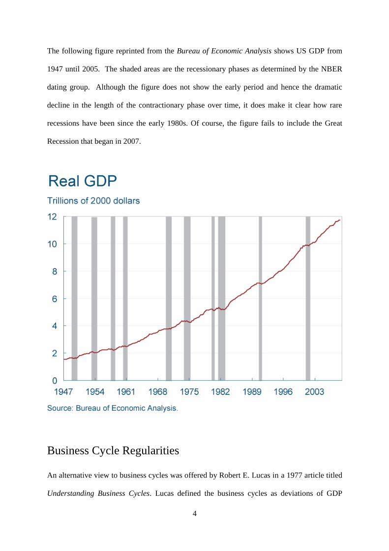
The following figure reprinted from the Bureau of Economic Analysis shows US GDP from

1947 until 2005. The shaded areas are the recessionary phases as determined by the NBER

dating group. Although the figure does not show the early period and hence the dramatic

decline in the length of the contractionary phase over time, it does make it clear how rare

recessions have been since the early 1980s. Of course, the figure fails to include the Great

Recession that began in 2007.

Business Cycle Regularities

An alternative view to business cycles was offered by Robert E. Lucas in a 1977 article titled

Understanding Business Cycles. Lucas defined the business cycles as deviations of GDP

5

about its trend. He further went on to define business cycle regularities to mean

comovements of deviations of other time series from their trends with the deviations of

output from its trend.

The reason Lucas gives for breaking with the traditional approach of dating the business

cycle is that economists going back to Eugen Slutzky (1927) have understood that that the

time series of GDP is well-approximated by a low order stochastic difference equation with a

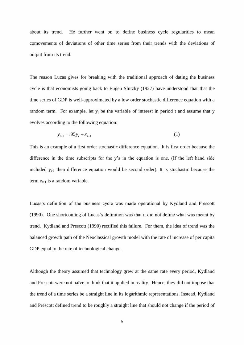
random term. For example, let yt be the variable of interest in period t and assume that y

evolves according to the following equation:

11 95. ttt yy (1)

This is an example of a first order stochastic difference equation. It is first order because the

difference in the time subscripts for the y’s in the equation is one. (If the left hand side

included yt-1 then difference equation would be second order). It is stochastic because the

term εt+1 is a random variable.

Lucas’s definition of the business cycle was made operational by Kydland and Prescott

(1990). One shortcoming of Lucas’s definition was that it did not define what was meant by

trend. Kydland and Prescott (1990) rectified this failure. For them, the idea of trend was the

balanced growth path of the Neoclassical growth model with the rate of increase of per capita

GDP equal to the rate of technological change.

Although the theory assumed that technology grew at the same rate every period, Kydland

and Prescott were not naïve to think that it applied in reality. Hence, they did not impose that

the trend of a time series be a straight line in its logarithmic representations. Instead, Kydland

and Prescott defined trend to be roughly a straight line that should not change if the period of

6

analysis were either shortened or lengthened and that should not involve any human

judgement.

The algorithm used by Kydland and Prescott to compute the trend of a time series and also its

deviations is known as the Hodrick-Prescott filter. The Hodrick-Prescott filter (HP) works

as follows: Let Yt be some variable at time t, and let yt be the logarithm of that variable at

time t. Let τt denote the trend (logarithm) of the variable. In the HP filter, the time series of yt

is known and the objective is to find the trend. The HP filter chooses the trend to minimize

the following

2

1

1

1

1

2 )]()[()(

t

T

t

ttt

T

t

tty (2)

The first terms is the sum of the squared deviations. The second term is effectively the

penalty or constraint associated with not having the trend be a linear function. The value of λ

determines the weight on the penalty term and determines the extent to which the trend is a

straight linear function. If we assign λ = +∞, then the penalty term has such a huge weight

that we will set (τt+1-τt )= (τt – τt-1), i.e. a straight line. If in contrast we assign λ=0, then the

trend is equal to output as there is no penalty with changing the slope of the trend line, i.e., yt

= τt.

For the purpose of detrending data at the quarterly frequency, the value that is assigned to λ

in the HP algorithm is 1600. If we were to use annual data, there is far less agreement as to

what is the appropriate value for the smoothing parameter. Some studies set λ = 6.5 whereas

others set λ = 100.

In documenting the business cycle properties, the first step is to find the trend of each time

series, {τt} and its deviations {dt=yt-τt}. The business cycle documentation focusses on three

7

aspects of the detrended data. The first is a measure of the amplitude, or size of the deviation

from its trend, the so called volatility. For this purpose the steps are to first express the

deviation as a percentage of the trend, namely, define xt = dt/τt. Next, we take the standard

deviation of the (percentage) deviation from trend. This is the measure of volatility. It is

measured as a percentage of the trend, not the absolute size of the deviation. This is

important to note as we shall see later on that investment as a percentage of its trend is about

3 times more volatile than GDP. In absolute terms, since investment is only about 25 percent

of GDP, its volatility is smaller.

The second property is the comovement of the deviations of each variable from its trend with

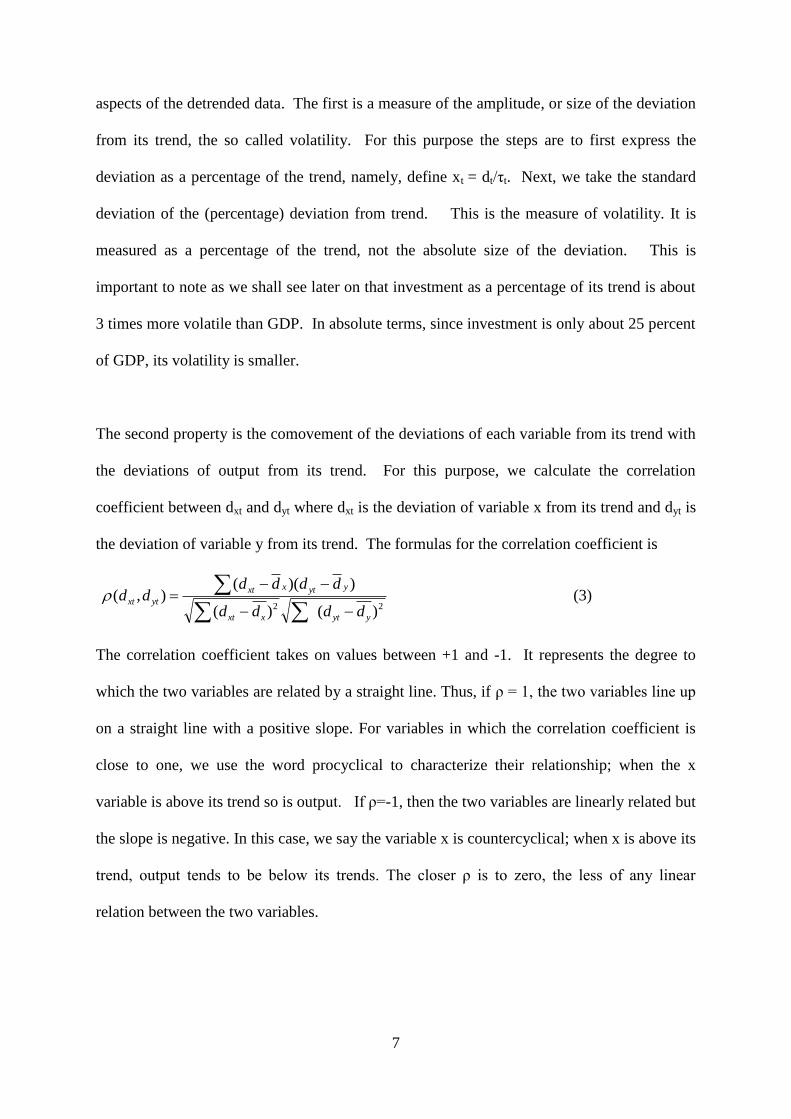
the deviations of output from its trend. For this purpose, we calculate the correlation

coefficient between dxt and dyt where dxt is the deviation of variable x from its trend and dyt is

the deviation of variable y from its trend. The formulas for the correlation coefficient is

22 )()(

))((),(

yytxxt

yytxxt

ytxt

dddd

dddddd

(3)

The correlation coefficient takes on values between +1 and -1. It represents the degree to

which the two variables are related by a straight line. Thus, if ρ = 1, the two variables line up

on a straight line with a positive slope. For variables in which the correlation coefficient is

close to one, we use the word procyclical to characterize their relationship; when the x

variable is above its trend so is output. If ρ=-1, then the two variables are linearly related but

the slope is negative. In this case, we say the variable x is countercyclical; when x is above its

trend, output tends to be below its trends. The closer ρ is to zero, the less of any linear

relation between the two variables.

8

The final measure in documenting the business cycle properties is also based on computing

correlation coefficients, but it is done with the intent of determining whether a variable leads

or lags the output series. For the purpose of determining if a series leads output we calculate

the correlation coefficient between dxt-j and dyt and for the purpose of determining if a series

lags output we calculate the correlation coefficient between dxt+j and dyt. The value of j

typically ranges between 1 and 4 when dealing with quarterly data. Thus, one is considering

lags and leads of one year or less.

The following tables are based on Kydland and Prescott (1990). Table 2 is organized around

the uses of GDP, namely, GDP=C+I+G+Nx. The most striking features of the table are

volatility of the investment time series. As seen in column 2, it is roughly 3 times more

volatile than output. Recall, that the volatility is not in absolute dollar terms but as a

percentage of a trend. With the exception of residential investment, each sub category of

investment is most strongly positively correlated with contemporaneous deviations in output,

or lags the cycle by a quarter. Residential Investment leads the cycle with by a quarter or half

year. This should not be surprising as Residential Investment, (i.e;, New Housing) is a

heavily referenced leading indicator in the news.

9

Table17.2

Cyclical behavior of U.S. output and income components(deviations from trend of product

and income variables, quarterly,1954-1989)

Variable x

Volatility

(% std.dev.)

Cross Correlation of Real GNP with

x(t-5) x(t-4) x(t-3) x(t-2) x(t-1) x(t) x(t+1) x(t+2) x(t+3) x(t+4) x(t+5)

Real Gross National Product 1.71 -0.03 0.15 0.38 0.63 0.85 1.00 0.85 0.63 0.38 0.15 -0.03

Consumption Expenditures 1.25 0.25 0.41 0.56 0.71 0.81 0.82 0.66 0.45 0.21 -0.02 -0.21

Nondurables and services 0.84 0.20 0.38 0.53 0.67 0.77 0.76 0.63 0.46 0.27 0.06 -0.12

Nondurables 1.23 0.29 0.42 0.52 0.62 0.69 0.69 0.57 0.38 0.16 -0.05 -0.22

Services 0.63 0.03 0.25 0.46 0.63 0.73 0.71 0.60 0.49 0.39 0.23 0.07

Durables 4.99 0.25 0.38 0.50 0.64 0.74 0.77 0.60 0.37 0.10 -0.14 -0.32

Investment Expenditures 8.30 0.04 0.19 0.39 0.60 0.79 0.91 0.75 0.50 0.21 -0.05 -0.26

Fixed Investment 5.38 0.09 0.25 0.44 0.64 0.83 0.90 0.81 0.60 0.35 0.08 -0.14

Nonresidential 5.18 -0.26 -0.13 0.05 0.31 0.57 0.80 0.88 0.83 0.68 0.46 0.23

Structures 4.75 -0.40 -0.31 -0.17 0.03 0.29 0.52 0.65 0.69 0.63 0.50 0.34

Equipment 6.21 -0.18 -0.04 0.14 0.39 0.65 0.85 0.90 0.81 0.62 0.38 0.15

Residential 10.89 0.42 0.56 0.66 0.73 0.73 0.62 0.37 0.10 -0.15 -0.34 -0.45

Government Purchases 2.07 0.00 -0.03 -0.03 -0.01 -0.01 0.05 0.09 0.12 0.17 0.27 0.34

Federal 3.68 0.00 -0.05 -0.08 -0.09 -0.09

-

0.02 0.03 0.06 0.10 0.19 0.24

State and Local 1.19 0.06 0.10 0.17 0.25 0.26 0.25 0.20 0.16 0.19 0.27 0.36

Exports 5.53 -0.50 -0.46 -0.34 -0.14 0.11 0.34 0.48 0.53 0.53 0.53 0.45

Imports 4.92 0.11 0.18 0.30 0.45 0.61 0.71 0.71 0.51 0.28 0.03 -0.19

Real Net National Income

Labor Income* 1.58 -0.18 -0.02 0.18 0.42 0.68 0.88 0.90 0.80 0.62 0.40 0.19

Capital Income** 2.93 0.10 0.24 0.44 0.63 0.79 0.84 0.60 0.30 0.02 -0.19 -0.29

Proprietors' Income and Misc.+ 2.70 0.11 0.24 0.38 0.55 0.62 0.68 0.46 0.29 0.11 0.02 -0.10

Personal Consumption Expenditures are also procyclical but less volatile than output. This

makes sense from the standpoint of theory. Consumer utility maximization is based on the

idea that individuals prefer smooth consumption streams. Interestingly, the durable

component category of Consumption Expenditures is as volatile as investment expenditures.

To the extent that household durable purchases are investment goods this finding is not

surprising.

10

Government expenditures show very little contemporaneous variation with the business

cycle. State and local government expenditures are more strongly procylical than

expenditures by the federal government. This makes sense in light of what we learned earlier

about the inability of state governments to print money and how this leads to US states

running fewer deficits than the Federal government. Imports are strongly procyclical.

Imported goods are bought by consumers and businesses and to the extent that consumption

expenditures and investment expenditures are procyclical, imports will be also procyclical.

The next Table is organized around the inputs and output of the economy. Importantly, labor

input as measured by total hours is less volatile than output and strongly procyclical. There

are two independent measures of total hours in the United States, Household surveys and

Establishment Surveys. The Household survey shows less volatility. The Household survey

also breaks total hours into employment and hours per worker. What is interesting to note

here is that employment is procyclical with a lag of one quarter whereas hours per worker is

contemporaneously procyclical. This suggests that firms respond initially to an increase in

demand for their product by having current workers work longer hours. They then respond

by adding workers with a three month lag.

11

Table17.1

Cyclical behavior of U.S. production inputs(deviations from trend of input variables,

quarterly,1954-1989)

Variable x

Volatility Cross Correlation of Real GNP with

(%

std.dev.) x(t-5) x(t-4) x(t-3) x(t-2) x(t-1) x(t) x(t+1) x(t+2) x(t+3) x(t+4) x(t+5)

Real Gross National Product 1.71 -0.03 0.15 0.38 0.63 0.85 1.00 0.85 0.63 0.38 0.15 -0.03

Labor Input

Hours (Household Survey) 1.47 -0.10 0.05 0.23 0.44 0.69 0.86 0.86 0.75 0.59 0.38 0.18

Employment 1.06 -0.18 -0.04 0.14 0.36 0.61 0.82 0.89 0.82 0.67 0.47 0.25

Hours per Worker 0.54 0.08 0.21 0.35 0.49 0.66 0.71 0.59 0.43 0.29 0.11 -0.02

Hours (Establishment Survey) 1.65 -0.23 -0.07 0.14 0.39 0.66 0.88 0.92 0.81 0.64 0.42 0.21

GNP/Hours (Household Survey) 0.88 0.11 0.21 0.34 0.48 0.50 0.51 0.21 -0.02 -0.25 -0.34 -0.36

GNP/Hours (Establishment Survey) 0.83 0.40 0.46 0.49 0.53 0.43 0.31 -0.07 -0.31 -0.49 -0.52 -0.50

Average Hourly Real Compensation

(Business Sector) 0.91 0.30 0.37 0.40 0.42 0.40 0.35 0.26 0.17 0.05 -0.08 -0.20

Capital Input

Nonresidental Capital Stock* 0.62 -0.58 -0.61 -0.51 -0.48 -0.31 -0.08 0.16 0.39 0.56 0.66 0.70

Structures 0.37 -0.45 -0.51 -0.55 -0.53 -0.44 -0.29 -0.10 0.09 0.25 0.38 0.45

Producers' Durable Equipment 0.99 -0.57 -0.58 -0.53 -0.41 -0.22 0.02 0.26 0.47 0.62 0.70 0.71

Inventory Stock (nonfarm) 1.65 -0.37 -0.33 -0.23 -0.05 0.19 0.50 0.72 0.83 0.81 0.71 0.53

The capital input show very little correlation with output is far less volatile. This makes

sense. Today, the capital stock is essentially fixed and cannot be increased or decreased

(although one can certainly keep equipment idle on the shelf. Although not

contemporaneously related to output deviations, the capital input has a strong positive

correlation with a lag of 1 year to 1.25 years. This makes sense in light of investment

expenditures being strongly and contemporaneously procyclical. It takes time to build new

machines and new structures.

The table also shows how output per work hour, a proxy for productivity, and average hourly

real compensation, a proxy for real wages) move with output. Each of these series is about

12

half as volatile as output and each is contemporaneously procyclical. At the time of the

article, these findings were surprising as they were in conflict with the predictions of the

Keynesian macro model of the pre-1970 era.

The final Table in the Kydland and Prescott article examines the volatility and correlations

between monetary variables. They consider three monetary aggregates: the monetary base,

M1 and M2. The monetary base consists of the total amount of currency either held in the

hands of the public or in a deposit of a commercial bank at the central bank. M1 consists of

money held by the public, travelers checks and demand deposits (i.e., checking accounts). M2

includes all of M1 plus savings deposits and time deposits less than $100,000. The monetary

base is the measure of the money supply that is central bank has most control of. M1 is the

value of financial assets that primarily serve as a medium of exchange. M2 includes the value

of financial assets that serve as a store of wealth. All are procyclical, but moderate in their

correlations. The strongest correlation is with M2 with a lead of one half to three fourths of a

year. For the price level, the key finding is that it is countercyclical; when output is above its

trend, prices are below its trend. Again, this is a finding that stands in sharp contrast to the

Keynesian model that had dominated the pre-1970 era.

13

Table17.4

Cyclical behavior of U.S. monetary aggregates and the price level(deviations from trend of

money stock, velocity, and price level, quarterly,1954-1989)

Variable x

Volatility

(% std.dev.)

Cross Correlation of Real GNP with

x(t-5) x(t-4) x(t-3) x(t-2) x(t-1) x(t) x(t+1) x(t+2) x(t+3) x(t+4) x(t+5)

Nominal Money Stock

Monetary Base 0.88 -0.12 0.02 0.14 0.25 0.36 0.41 0.40 0.37 0.32 0.28 0.26

M1 1.68 0.01 0.12 0.23 0.33 0.35 0.31 0.22 0.15 0.09 0.07 0.07

M2 1.51 0.48 0.60 0.67 0.68 0.61 0.46 0.26 0.05 -0.15 -0.33 -0.46

M2-M1 1.91 0.53 0.63 0.67 0.65 0.56 0.40 0.20 -0.01 -0.21 -0.39 -0.53

Velocity*

Monetary Base 1.33 -0.26 -0.15 0.00 0.22 0.40 0.59 0.50 0.37 0.22 0.08 -0.08

M1 2.02 -0.24 -0.19 -0.12 -0.01 0.14 0.31 0.32 0.27 0.20 0.10 0.00

M2 1.84 -0.63 -0.59 -0.48 -0.29 -0.05 0.24 0.34 0.40 0.43 0.44 0.43

Price Level

Implicit GNP Deflator 0.89 -0.50 -0.61 -0.68 -0.69 -0.64 -0.55 -0.43 -0.31 -0.17 -0.04 0.09

Consumer Price Index 1.41 -0.52 -0.63 -0.70 -0.72 -0.68 -0.57 -0.41 -0.24 -0.05 0.14 0.30

There is much debate whether monetary policy has real effects on the economy. Although

M2 was found to leads real GDP in the 1954-89 period, this does not mean that changes in

the money supply cause changes in real output. The numbers in the table are correlations,

and hence do not say anything about causation. In fact, King and Plosser argued that the

positive lead documented by Kydland and Prescott could actually reflect causation from

future output to M2, what is called reverse causation.

Basically, the story is that people understand or believe that the economic activity will pick

up in three months or six months from now. As a result, they may want to take out a loan to

buy a new suit, or extra uniform so they can be ready for the upturn. If banks were holding

excess reserves, currency in their own vaults or the central bank’s vault above the legal

14

requirement, they can meet this increase in demand for loans with these funds. How much

money there is in the economy depends on the behaviour of both households as to how much

money they hold in their pocket and banks as to how many excess reserves they hold. If

households put less money in their pockets and more in their checking or savings accounts

and if banks hold less excess reserves, the money supply will be higher given the same

monetary base.

Conclusion

To be written

Appendix: Installing the Hodrick-Prescott Filter

Kurt Annen has written a free-download of the HP-Filter for Excel.

To add the HP filter to your excel spreadsheet first go to the web page: http://www.web-

reg.de/hp/hp.htm. From there, follow the instruction to download the HP filter to your

computer. The files will be installed in zip file. Open the file "hpfilter.zip" and extract the

three files within. Then open the file "HP-Example.xls" and follow the instructions to install.

(Note: that for Microsoft Excel 2010 you will have to go File – Options- Add-Ins as there is

no Tools Menu)

Using the HP Filter in Excel After installing the HP filter in excel, you are ready to detrend any time series using the

function HP(). (The St. Louis Federal Reserves website (FRED) is a great site to easily input

data into an excel spreadsheet. You can download the Add-In ) We illustrate the use of the

HP Filter data for a time series that appears in cells A2:A17 in an excel spreadsheet. You can

watch a video on the using the HP-Filter by Humberto Barreto.

15

Don’t forget to use the logarithm of the time series you want to detrend before Steps1-4.

Step1: Select the block of cells that we want to apply the HP filter to. To compute the trend

component in column C, press the Shift key and place the mouse cursor on cell C2 then click

cell C17. Make sure the length of the block is identical to the data A2:17.

Step2: Next type in “hp( “ in the formula bar.

16

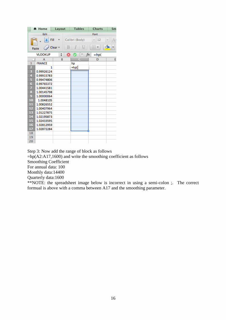
Step 3: Now add the range of block as follows

=hp(A2:A17,1600) and write the smoothing coefficient as follows

Smoothing Coefficient

For annual data: 100

Monthly data:14400

Quarterly data:1600

**NOTE: the spreadsheet image below is incorrect in using a semi-colon ;. The correct

formual is above with a comma between A17 and the smoothing parameter.

17

Step4: Hit the enter key while pressing Shift key and Control key at the same time.

Finally, we get the result. Recall that the hp function returns the trend. To find the deviation,

you would subract C2 from A2.

18

Problem Set: Use the St. Louis Federal Reserve Bank’s data website called FRED to input

the following data for the US economy into an excel spreadsheet. Choose quarterly data.

Use the Browse Popular Data Releases

Under Gross Domestic Product Icon Download

1. Real GDP (from 1948)

2. Real Personal Consumption Expenditures (from 1948)

3. Real Gross Private Domestic Investment (from 1948)

Under Browse Popular US Data

Under Population, Employment and Labor markets download

1. Unemployment rate (from 1948)

Under Prices download

1. GDP Implicit Price Deflator (from 1948)

Under Money, Banking and Finance download

1. M2 (Starting with 1991)

You are to:

HP Filter each series using the smoothing parameter =1600.

Hand in for each series

1. Volatility

2. Correlation coefficient with deviations in output.