holographic algorithms without matchgates

HOLOGRAPHIC ALGORITHMS WITHOUT MATCHGATES

J.M. LANDSBERG, JASON MORTON AND SERGUEI NORINE

Abstract. The theory of holographic algorithms, which are polynomial time algorithms forcertain combinatorial counting problems, surprised the complexity community by showing cer-tain problems, very similar to #P complete problems, were in fact in the class P. In particular,the theory produces algebraic tests for a problem to be in P. In this article we describe thegeometric basis of these algorithms by (i) replacing the construction of graph fragments in theprocedure by the direct contstruction of a skew symmetric matrix, and (ii) replacing the com-putation of weighted perfect matchings of an auxilary graph by computing the Pfaffian of thedirectly constructed skew-symmetrix matrix. This procedure indicates a more geometric ap-proach to complexity classes. It also leads to more general constructions where one replaces the“Grassmann-Plucker identities” which test for admissibility by other algebraic tests. Naturalproblems treatable by these methods have been previously considered in a different context, andwe present one such example.

1. Introduction

1.1. History. In [19, 20, 21, 23, 24, 25] L. Valiant introduced matchgates and holographic algo-rithms, in order to prove the existence of polynomial time algorithms for counting and sum-of-products problems that naıvely appear to have exponential complexity. Such algorithms havebeen studied in depth and further developed by J. Cai et al. [1, 2, 3, 4, 5, 6, 7, 8].

The determinant of an n× n matrix, expressed as a sum of terms indexed by the symmetricgroup Sn, has n! terms, yet it can be computed in polynomial time. Holographic algorithmsare a particular strategy for finding algorithms which provide efficient computation of suchexponential sums of products by essentially expressing the problem as a determinant. Someexploit a “Hadamard-type” change of basis inspired by quantum computation and this “su-perposition,” together with the cancellation effect present in the determinant, is the source ofthe name. Holographic algorithms have also been called “accidental algorithms” because theysometimes provide a polynomial time algorithm for certain parameter values in a parameterizedfamily of problems, and these problems are NP-hard (e.g. because they are ⊕P complete) or#P-complete for other parameter values.

For the reader not familiar with complexity theory, a typical problem considered in complexitytheory is as follows: let x1, . . . , xn be a collection of Boolean variables (i.e., variables assumingthe values “true” or “false”) and let c1, . . . , cp be a collection of clauses (e.g., x1 ∧ ( x3)). Thenone wants to count the number of satisfying assignments. A geometer might wish to view the xjas taking values in the field with two elements F2, the cs as equations on Fn2 , and the problemis to count the number of points of the variety determined by the cs. Such a problem is called#SAT in the complexity literature. (The # refers to counting, if it is left off, the problem isjust to determine if there exists any satisfying assignment.)

Often restrictions are placed on the types of clauses allowed. Typical restrictions (with theirnames) are

(1) 3SAT: Each clause involves only three variables.

Date: December 7, 2011.

1

2 J.M. LANDSBERG, JASON MORTON AND SERGUEI NORINE

(2) CNF: conjunctive normal form, i.e., a collection of “or” clauses joined together with aseries of “ands” e.g., (x1 ∨ x3) ∧ (x2 ∨ x5 ∨ x4) ∧ (x7).

(3) Mon: restriction to monotone clauses - variables appearing in a clause either all appearpostively or all negatively.

(4) Rtw: read twice - each variable appears in just two clauses.(5) NAE: all clauses are “not all equal”- variables appearing in the same clause are not all

allowed to have the same assignments.(6) Pl: planar: the variable-clause inclusion graph (see below) constructed from each in-

stance is planar

Problems are named after these restrictions, for example #Pl-Rtw-Mon-3CNF (defined in [22])is to count the number of satisfying assignments when clauses are subject to the restrictionsPl-Rtw-Mon-3CNF. For this problem, even counting the number of solutions mod 2 is ⊕Pcomplete (this problem is called #2Pl-Rtw-Mon-3CNF) and therefore NP-hard by Valiant-Vazirani reduction [26]. Nevertheless, a holographic algorithm shows that counting the numberof solutions to #Pl-Rtw-Mon-3CNF mod 7 (called #7Pl-Rtw-Mon-3CNF) can be accomplishedin polynomial time [22].

Remark 1.1. Note that all the conditions above except the last are “local”. The global natureof the last condition turns out to be crucial for implementation of holographic algorithms.

The perspective provided by holographic algorithms relates the computational complexity ofcertain key problems with the solvability of systems of polynomial equations [22]. A popularaccount describing holographic algorithms can be found in [11].

Holographic algorithms work as follows: suppose the problem P is SAT or some restrictedversion of SAT. Say an instance P of P has variables x1, . . . , xm subject to clauses c1, . . . , cp.

(1) Associate to P a bipartite graph ΓP = (V,U,E), with vertex sets V = x1, . . . , xm andU = c1, . . . , cp. Draw an edge (i, s) ∈ E iff xi appears in cs.

(2) Associate (two dimensional) vector spaces Ae, equipped with bases, to each edge, “local”tensors to each vertex, and a “global” tensor to each vertex set, such that the two global

tensors lie in dual vector spaces. Write G ∈ ⊗e∈EAe ∼ C2|E| , R ∈ ⊗e∈EA∗e for the globaltensors. The construction is such that the pairing 〈G,R〉 ∈ C counts the number ofsatisfying assignments (so the pairing actually takes values in the nonnegative integers).This step is explained in §2.

(3) Perform a (cheap) basis change in each Ae and the dual basis change in each A∗e suchthat local matchgate identities are satisfied. The matchgate identities are a collectionof polynomial equations in the coordinates of the clauses and variables. This step isexplained in §3.

(4) Replace the vertices of ΓP with weighted graph fragments to obtain a new weightedgraph ΓΩ(P ) such that the weighted sum of perfect matchings of ΓΩ(P ) equals 〈G,R〉.The weighted graph fragments are called matchgates.

(5) Assuming ΓΩ(P ) is planar (or more generally Pfaffian), compute the weighted sum ofperfect matchings of ΓΩ(P ) quickly using the FKT algorithm [14, 18]. The FKT algorithmfor weighted planar graphs is a way to alter signs of weights to convert the Hafnian (whichcounts the number of perfect matchings of a weighted graph), to a Pfaffian, which isequivalent in complexity to the determinant.

In the early matchgates literature the construction of the matchgate graph fragments wasviewed as an “art”, but since then, a library of such constructions has been made by Cai et. al.at least for vertices without too many edges, so it is also essentially algorithmic to apply. Thematchgate identities are equalities among sums of products of sub-Pfaffians. We discuss themmore below.

HOLOGRAPHIC ALGORITHMS WITHOUT MATCHGATES 3

1.2. Holographic algorithms without matchgates. Our approach, described in §4, replacessteps (4) and (5) with the computation of the Pfaffian of a natural |E| × |E| matrix associatedto the original graph ΓP . We present an algorithmic construction of a small matrix for eachvariable and clause, which is the analog of the matchgate construction.

We replace FKT with an edge ordering defined by a plane curve as described in Section 5.Both FKT and our edge ordering have the effect of “making the signs work out right”.

The Valiant-Cai formulation of holographic algorithms can be summarized as

(1) #satisfying assignments of P = 〈G,R〉 = weighted sum of perfect matchings of ΓΩ(P ).

We associate constants α = αG, β = βR (depending only on the number of each type ofvertex) and |E| × |E|-skew symmetric matrices z = zG, y = yR directly to G, R, without theconstruction of matchgates, to obtain the equality:

(2) #satisfying assignments of P = 〈G,R〉 = αβPfaff(z + y);

see Examples 4.8 and 4.9. The constants and matrices are essentially just components of thevectors G,R. The algorithm complexity is dominated by evaluating the Pfaffian of the |E|× |E|skew-symmetric matrix.

The key to our approach is that a vector satisfies the matchgate identities iff it is a vector ofsub-Pfaffians of some skew-symmetric matrix, and that the pairing of two such vectors can bereduced to calculating a Pfaffian of a new matrix constructed from the original two. A similarphenomenon holds in greater generality discussed in Appendix 7. A simple example is the setof vectors of sub-minors of an arbitrary rectangular matrix. We describe an example of such animplementation in Section 6.

The starting point of our investigations was the observation that the matchgate identitiescome from classical geometric objects called spinors. The results in this article do not requireany reference to spinors to either state or prove, and for the convenience of the reader notfamiliar with them we have eliminated all mention of them except for this paragraph and anAppendix (§7) included for the interested reader.

The purpose of this paper is to facilitate an understanding of the geometric basis of holographicalgorithms. It does not address such issues as implementation, the construction of explicit newalgorithms, or dependence on the ground field. The first two topics are addressed in [15]. Thethird is beyond our expertise, but since the circulation of this paper in preprint form, A. Snowdenhas begun to work on this issue.

2. Counting problems as tensor contractions

For brevity we continue to restrict to problems counting the number of satisfying assign-ments of Boolean variables xi subject to clauses cs (such as #Pl-Mon-NAE-SAT defined above).Following e.g., [2] express an instance P of such a problem in terms of a tensor contractiondiagrammed by a planar bipartite graph ΓP = (V,U,E) as above (see Figure 1), together withthe data of tensors Gi = Gxi and Rs = Rcs attached at each vertex xi ∈ V and cs ∈ U . Gi willrecord that xi is 0 or 1 and Rs will record that the clause cs is satisfied. Let n = |E| be thenumber of edges in ΓP .

For each edge e = (i, s) ∈ E define a 2-dimensional C vector space Ae with basis ae|0, ae|1.Say xi has degree di and is joined to cj1 , . . . , cjdi . Let Ei denote the set of edges incident to xiand associate to each xi the tensor

Gi :=ai,sj1 |0⊗ · · ·⊗ ai,sjdi |0 + ai,sj1 |1⊗ · · ·⊗ ai,sjdi |1 ∈ Ai := Aisj1⊗ · · ·⊗ Aisjdi(3)

= ⊗e∈Ei

ae|0 + ⊗e∈Ei

ae|1


The tensor Gi represents that either xi is true (all 1’s) or false (all 0’s), and presents the samevalue to each clause. It is called a generator in the matchgates literature and is denoted by theco-ordinate vector (1, 0, . . . , 0, 1) corresponding to a lexicographic basis of Ai = ⊗e∈Ei Ae. Thisvector is called its signature. We use notation emphasizing the tensor product structure of the

vector space Ai = C2di , and will use the word signature to refer to the tensor expression of Gi.Next define a tensor associated to each clause cs representing that cs is satisfied. Let A∗e be

the dual space to Ae with dual basis αe|0, αe|1. Let Es denote the set of edges incident to cs.For example, if cs has degree ds and is “not all equal” (NAE), then the corresponding tensor(called a recognizer) associated to it is

(4) Rs :=∑

(ε1,...,εds )6=(0,...,0),(1,...,1)

αi,s1|ε1⊗ · · ·⊗ αi,sds |εds =∑

(ε1,...,εds )6=(0,...,0),(1,...,1)

⊗e∈Es

αe|εe

Remark 2.1. Our restriction to #-NAE-3SAT is to facilitate presentation. It is already # Phard.

Now consider G :=⊗iGi and R :=⊗sRs respectively elements of the vector spaces A :=⊗eAeand A∗ := ⊗eA∗e. Then the number of satisfying assignments to P is 〈G,R〉 where 〈·, ·〉 :A × A∗ → C is the pairing of dual vector spaces. At this point we have merely exchanged ouroriginal counting problem for the computation of a pairing in vector spaces of dimension 2|E|.

G1ONMLHIJK

1111111111

A1

G2ONMLHIJK

1111111111

A2⊗A4

G3ONMLHIJKA3

R1

ttttttttttttttt

A∗1⊗A∗2⊗A∗3

R2

A∗4

Variable Vertices V

Edges E

Clause Vertices U

G = G1⊗G2⊗G3 ∈ A1⊗A2⊗A3⊗A4

R = R1⊗R2 ∈ A∗1⊗A∗2⊗A∗3⊗A∗4

1 2 34

Figure 1. A bipartite graph Γ diagrams a tensor contraction, representing anexponential sum of products such as counting the satisfying assignments of asatisfiability problem. Boxes denote clauses, circles denote variables. Each clauseor variable corresponds to a tensor lying in the indicated vector space; e.g. R1 ∈A∗1⊗A∗2⊗A∗3. Instead of replacing each vertex with a matchgate, our constructiondefines an n × n matrix, where n is the number of edges in the problem graph.The Pfaffian of this matrix, times a constant depending on the number of eachtype of variable and clause, is the number of satisfying assignments.

3. Local conditions and change of basis

In order to be able to construct the matchgates corresponding to the xi, cs, there are localconditions that need to be satisfied; the algebraic equations placed on the Gi, Rs are called theGrassmann-Plucker identities (or Matchgate Identities in this context). See, e.g., Theorem 7.2of [4] for an explicit expression of the equations, which date back at least to Chevalley in the1950’s [9]. From our perspective, these identities ensure that a tensor T representing a variableor clause can be written as a vector of sub-Pfaffians of some matrix. From the matchgatespoint of view, these equations are necessary and sufficient conditions for the existence of graphfragments that can replace the vertices of ΓP to form a new weighted graph ΓΩ(P ) such that theweighted perfect matching polynomial of ΓΩ(P ) equals 〈G,R〉.


Expressed in the basis most natural for a problem, a clause or variable tensor may fail tosatisfy the Grassmann-Plucker identities. However it may do so under a change of basis; e.g. inExample 3.1 below, we replace the basis (True, False) with (True+False, False−True). Such achange of basis will not change the value of the pairing A × A∗ → C as long as we make thecorresponding dual change of basis in the dual vector space—but of course this may cause thetensors in the dual space to fail to satisfy the identities. Thus one needs a change of basis thatworks for both generators and recognizers. In this article, as in almost all existing applicationsof the theory, we only consider changes of bases in the individual Ae’s, and we will perform theexact same change of basis in each such, although neither restriction is a priori necessary forthe theory.

Remark 3.1. While it may seem incredible that such changes of basis might exist for a problem,in fact for many NP-hard problems there exist local changes of basis that work for the Gi andfor the Rs. Moreover the local changes for the Gi can be glued together to make a global changethat works for the tensor G, and the local changes for the Rs can be glued together to make aglobal change that works for the tensor R. The “only”problem that occurs is a compatibility ofsigns, which needs a global condition such as planarity to be overcome.

3.1. Example. In #Mon-3-NAE-SAT the generator tensor Gi corresponding to a variable ver-tex xi is (3). The recognizer tensor corresponding to a NAE clause Rs is (4) and in our case wewill have ds = 3 for all s.

Let T0 be the basis change, the same in each Ae, sending ae|0 7→ ae|0+ae|1 and ae|1 7→ ae|0−ae|1which induces the basis change αe|0 7→ 1

2(αe|0 +αe|1) and αe|1 7→ 12(αe|0−αe|1) in A∗e. This basis

is denoted b2 in [25]. Applying T0, we obtain

T0(ai,si1 |0⊗ · · ·⊗ ai,sidi |0+ai,si1 |1⊗ · · ·⊗ ai,sidi |1) = 2∑

(ε1,...,εdi )|∑ε`=0 (mod 2)

ai,si1 |ε1⊗ · · ·⊗ ai,sidi |εdi .

In the matchgates literature this tensor is denoted by the vector (2, 0, 2, 0, . . . , 2, 0, 2) (assumingthe number of incident edges is even). The action on recognizer tensors is

T0

∑(ε1,ε2,ε3)6=(0,0,0),(1,1,1)

αi,s1|ε1⊗αi,s2|ε2⊗αi,s3|ε3

= 6αi,s1|0⊗αi,s2|0⊗αi,s3|0 − 2(αi,s1|0⊗αi,s2|1⊗αi,s3|1 + αi,s1|1⊗αi,s2|0⊗αi,s3|1 + αi,s1|1⊗αi,s2|1⊗αi,s3|0)

or, denoted by its co-ordinate vector, (6, 0, 0, 0,−2,−2,−2, 0).

4. Holographic algorithms without matchgates

4.1. Detour: Elementary identities from linear algebra. Our approach to holographicalgorithms essentially boils down to two simple identities from linear algebra. First, if x, y arematrices whose product is a square matrix, then

det(Id+ xy)

may be expressed as a sum of products of determinants of the square submatrices of x and y.Second is the even more elementary identity for block diagonal matrices

det

(X 00 Y

)= det(X) det(Y ).

More precisely, we use the Pfaffian analogs of these identities. The first is the key to performingthe pairing A× A∗ → C mentioned above in polynomial time, the second is the key to passingfrom the local changes of bases to a global change of basis.


4.2. The complement pairing and representing G and R as vectors of sub-Pfaffians.Assume we have a problem expressed as in §2 and have constructed tensors G,R such that insome change of basis their component tensors Gi, Rs satisfy the Grassmann-Plucker identities.For the purposes of exposition, we will assume the total number of edges is even. See thediscussion in the Appendix §7 for the case of an odd number of edges.

To compute 〈G,R〉, we will represent G and R as vectors of sub-Pfaffians. For an n × nskew-symmetric matrix z, the vector of sub-Pfaffians sPf(z) lies in a vector space of dimensionC2n , where the coordinates are labeled by subsets I ⊂ [n], and

(sPf(z))I = Pfaff(zI)

where zI is the submatrix of z including only the rows and columns in the set I. Letting

IC = [n] \ I, similarly define sPf∨

: Matn×n → C2n by

(sPf ∨(z))I = Pfaff(zIC ).

The vector spaces A = ⊗Ae, A∗ = ⊗A∗e come equipped with un-ordered bases induced fromthe bases of the Ae. These bases do not have a canonical identification with subsets of (1, . . . , n)but do have a convenient choice of identification after making a choice of edge ordering. Afteran ordering E of the edges has been chosen we obtain ordered bases of A,A∗. To obtain theconvenient choice of identification for A, identify the vector corresponding to I = (i1, . . . , i2p)with the element with 1’s in the i1, . . . , i2p slots and zeros elsewhere, so, e.g. I = ∅ correspondsto (0, . . . , 0), ..., I = (1, . . . , n) corresponds to (1, . . . , 1). (Recall we are assuming n is even.)Reverse the correspondence for A∗.

For later use, we remark that with these identifications, as long as the first (resp. last) entryof G (resp. R) is non-zero, we may rescale to normalize them to be one. (If say, e.g., the firstentry of G is zero but the last is not, and last entry of R is non-zero, we can just reverse theidentifications and proceed.) Note that the first and last choices of entries are independent ofthe edge ordering, but if necessary, to get the first and last entries non-zero, we simply take aless convenient choice of identification. (See §7 for an explanation of this freedom.) As long asthis is done consistently it will not produce any problems.

We now explicitly construct the matrices which play the role of matchgates. Suppose Gi is thegenerator tensor representing a single variable of degree d and that Gi satisfies the matchgateidentities. Possibly rescaling Gi by some factor α, we may assume that the coefficient of thelexicographically first term (supressing the i index in the notation for the rest of this paragraph)aε1|0⊗ · · ·⊗aεd|0 is 1.

Let 1 ≤ j<k ≤ d and consider the(d2

)generator tensors Gi, with ones (aεj |1) in the (j, k)-th

place and zeros (aεr|0) elsewhere. Let cjk denote the coefficient of these Gi’s. Let x be the d× dskew-symmetric matrix with xjk = cjk and xkj = −cjk. The matchgate identities, see e.g., [4,

Thm. 7.2], imply that for any (i1, i2, . . . , id) ∈ 0, 1d, the coefficient of aε1|i1⊗ · · ·⊗aεd|id in Giequals the Pfaffian of the principal submatrix of x including the rows where i` = 1 and excludingthose where i` = 0. We write sPf(x) = Gi. The construction is analogous for recognizers. Forexample, j = 2, k = 3 gives the term c23aε1|0⊗aε2|1⊗aε3|1⊗aε4|0 . . .⊗aεd|0.

For the rest of this section, we restrict attention to generator and recognizer tensors at thevertices that can be written Gi = sPf(xi) and Rs = sPf∨(ys) for matrices xi, ys, possibly aftera change of basis. We also assume for brevity that the Gi and Rs are symmetric, i.e. thatGi = sPf(xi) = sPf(π(xi)) for any permutation π on the edges incident on Gi; this covers manyproblems of interest. For the more general case when the variables or clauses are not symmetric,and we need to be more careful about defining EG and ER, see §5 and the Appendix §8.


Definition 4.1. Suppose a graph Γ has n edges. An edge order is a bijective labelling of theedges of Γ by the integers 1, 2, . . . , n. Call an edge order such that edges incident on each xi ∈ V(resp. cs ∈ U) have a consecutive block of labels a generator order (resp. recognizer order) anddenote such by EG (resp. ER).

Proposition 4.2. Suppose P is an instance of a problem expressed as a pairing such that EGand ER are respectively generator and recognizer orders to the graph ΓP . If for all xi ∈ V thereexists zi ∈ Matdi×di such that sPf(zi) = Gi under the EG order, and similarly, there existsys ∈Matds×ds for cs and Rs with sPf∨(ys) = Rs, then there exists z, y ∈Mat|E|×|E| such that

sPf(z) = G with the EG order and

sPf∨(y) = R with the ER order.

In this situation, z, y are just given by stacking the component matrices zi, ys block-diagonally.

Proof. The Pfaffian of a block-diagonal skew-symmetric matrix is the product of the Pfaffiansof the diagonal blocks.

As the proposition suggests, a difficulty appears when we try to find an order E that worksfor both generators and recognizers.

Definition 4.3. An order E is valid if there exists skew-symmetric matrices z, y such thatsPf(z) = G and sPf ∨(y) = R under the E order.

Thus if an order is valid〈G,R〉 =

∑I

PfaffI(z)PfaffIc(y)

and in the next subsection we will see how to evaluate the right hand side in polynomial time.Then in §5 we prove that if ΓP is planar, there is always a valid ordering.

4.3. Evaluating the complementary pairing of vectors of sub-Pfaffians. Let n be even.For an even set I ⊆ [n], define σ(I) =

∑i∈I i, and define sgn(I) = (−1)σ(I)+|I|/2. Proofs of the

following lemma can be found in [17, p. 110] and [12, p. 141].

Lemma 4.4. Let z and y be skew-symmetric n× n matrices. Then

Pfaff(z + y) =∑I⊆[n],

|I|≡0mod 2

sgn(I)PfaffI(z)PfaffIc(y)

To use Lemma 4.4 to compute inner products we need to adjust one of the matrices to correctthe signs. For a matrix z define a matrix z by setting zij = (−1)i+j+1zij . Let z be an n × nskew-symmetric matrix. Then for every even I ⊆ [n],

PfaffI(z) = sgn(I)PfaffI(z).

For odd |I|, both sides are zero. For |I| = 2p, p = 1, . . . , bn2 c,

PfaffI(z) = (−1)i1+i2+1 · · · (−1)i2p−1+i2p+1PfaffI(z) = sgn(I)PfaffI(z).

Thus we have the following Theorem.

Theorem 4.5. Let z, y be skew-symmetric n× n matrices. Then

〈sPf(z), sPf ∨(y)〉 = Pfaff(z + y).

In Section 5 we show that if ΓP is planar there is an easily computable valid edge orderingE. Our result may be summarized as follows:

Definition 4.6. Define a problem P to be holographic-friendly if for each instance P of P


(1) There exists a change of basis in C2 after which all the Gi = αi sPf(xi), Rs = βs sPf∨(yi)satisfy the Grassmann-Plucker identities with complementary indexing.

(2) There exists a valid edge order E.

Theorem 4.7. Let P be an instance of a holographic friendly problem P. Perform the desiredchange of basis and write Gi = αi sPf(xi), Rs = βs sPf∨(yi) for the generator and recognizertensors.

Let α =∏i αi and β =

∏s βs. Consider skew symmetric matrices x, y where xij is the

entry of α−1G E-corresponding to I = (i, j) and yij is the entry of β−1τ(R) E-corresponding to

Ic = (i, j). Then the number of satisfying assignments to P is given by αβPfaff(x+ y).

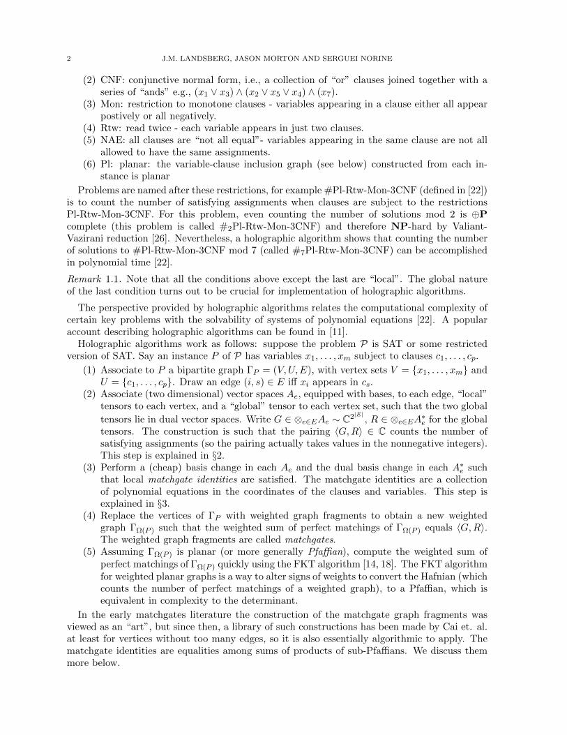
Example 4.8. Figure 2 shows an example of #Pl-Mon-3-NAE-SAT, with an edge order givenby a path through the graph. The corresponding matrix, z + y is below. In a generator order,

?>=<89:;

?>=<89:;?>=<89:;

?>=<89:;?>=<89:;

?>=<89:;

8

9 11

10

12

2

7 6

4

5 3

1

12

4

3

6

57

8

10

9

12

11

VVVV

VVVV

(a) (b)

Figure 2. Example 4.8, and the term S = (1, 2)(3, 6)(4, 5)(7, 8)(9, 12)(10, 11) inthe Pfaffian (which has no crossings). Circles are variable vertices and rectanglesclause vertices.

each variable corresponds to a(

0 1−1 0

)block. In a recognizer order, each clause corresponds to

a 3 × 3 block with −1/3 above the diagonal. Sign flips z 7→ z occur in a checkerboard patternwith the diagonal flipped; here no flips occur. We pick up a factor of 6

23for each clause and 2

for each variable, so α = 26, β = ( 623

)4, and αβPfaff(z + y) = 26 satisfying assignments.

z + y =

0 1 0 0 0 0 0 0 0 0 −1/3 −1/3−1 0 −1/3 −1/3 0 0 0 0 0 0 0 00 1/3 0 −1/3 0 1 0 0 0 0 0 00 1/3 1/3 0 1 0 0 0 0 0 0 00 0 0 −1 0 −1/3 −1/3 0 0 0 0 00 −1 0 0 1/3 0 −1/3 0 0 0 0 00 0 0 0 1/3 1/3 0 1 0 0 0 00 0 0 0 0 0 −1 0 −1/3 −1/3 0 00 0 0 0 0 0 0 1/3 0 −1/3 0 10 0 0 0 0 0 0 1/3 1/3 0 1 0

1/3 0 0 0 0 0 0 0 0 −1 0 −1/31/3 0 0 0 0 0 0 0 −1 0 1/3 0

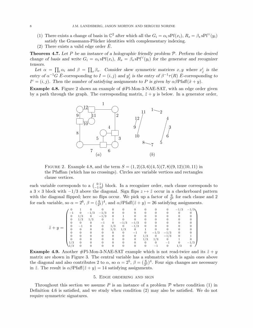
Example 4.9. Another #Pl-Mon-3-NAE-SAT example which is not read-twice and its z + ymatrix are shown in Figure 3. The central variable has a submatrix which is again ones abovethe diagonal and also contributes 2 to α, so α = 25, β = ( 6

23)4. Four sign changes are necessary

in z. The result is αβPfaff(z + y) = 14 satisfying assignments.

5. Edge ordering and sign

Throughout this section we assume P is an instance of a problem P where condition (1) inDefinition 4.6 is satisfied, and we study when condition (2) may also be satisfied. We do notrequire symmetric signatures.


?>=<89:;

?>=<89:;

?>=<89:;

?>=<89:;

?>=<89:;

5 6

1 3

10 9

8

7

2

4

11

12

0 1 −1 1 0 0 0 0 0 0 −1/3 −1/3−1 0 1 −1 0 0 0 0 −1/3 −1/3 0 01 −1 0 1 0 0 −1/3 −1/3 0 0 0 0−1 1 −1 0 −1/3 −1/3 0 0 0 0 0 00 0 0 1/3 0 −1/3 0 0 0 0 0 10 0 0 1/3 1/3 0 1 0 0 0 0 00 0 1/3 0 0 −1 0 −1/3 0 0 0 00 0 1/3 0 0 0 1/3 0 1 0 0 00 1/3 0 0 0 0 0 −1 0 −1/3 0 00 1/3 0 0 0 0 0 0 1/3 0 1 0

1/3 0 0 0 0 0 0 0 0 −1 0 −1/31/3 0 0 0 −1 0 0 0 0 0 1/3 0

Figure 3. Another #Pl-Mon-3-NAE-SAT example and its z + y matrix.

Given an order E we would like to know if it is valid, i.e., the signs can be made to workout right. Say EG, ER are generator and recognizer orders so that there exist skew-symmetricmatrices z, y such that with respect to these orders G = sPf(z), R = sPf(y). Let π, τ ∈ S|E|respectively be the permutations such that

(5) π(EG) = E and τ(ER) = E.

Then for all J ⊂ [n], Pfaffπ(J)(π(z)) = sgn(π|J)PfaffJ(z) and similarly for τ , so G and R arevectors of sub-Pfaffians except that possibly some signs are wrong. Valid orderings yield π, τwhich preserve sub-Pfaffian signs.

We describe one type of valid ordering for planar graphs, called a C-ordering. For anyplanar bipartite graph ΓP , a plane curve C intersecting every edge once corresponds to a non-self-intersecting Eulerian cycle in the dual of ΓP and can be computed in O(|E|) time. Fixsuch a C, an orientation and a starting point for C, and let EC be the order in which theresulting path crosses the edges of ΓP . Define ECG to be the generator order chosen so that thepermutation π : ECG → EC is lexicographically minimal. In particular, ECG agrees with EG onthe edges incident to any fixed generator in V . For example, the generator order on Figure 2 is1, 2, 3, 6, 4, 5, 7, 8, 9, 12, 10, 11. Define ECR similarly.

To show that EC is valid we will need another characterization of the sub-Pfaffians and thenotion of crossing number. Let S = (e1, e

′1), . . . , (ek, e

′k) be a partition of an ordered set I,

with |I| = 2k, into unordered pairs. Assume, for convenience, that er < e′r for 1 ≤ r ≤ k. Definethe crossing number cr(S) of S as

cr(S) = #(r, s) | er < es < e′r < e′s.Note that cr(S) can be interpreted geometrically as follows. If the elements of I are arranged ona circle in order and the pairs of elements corresponding to pairs in S are joined by straight-lineedges, then cr(S) is the number of crossings in the resulting geometric graph (see Figure 2(b)).When the order E on I is unclear from context we write cr(S, E), instead of cr(S).

For I ⊆ E(Γ), denote by ΓI the subgraph of Γ induced by I. Let S (ΓI) be the set ofpairings S = (e1, e

′1), . . . , (ek, e

′k) of I such that edges in each pair share a vertex in the set

V of generators. In other words, (ei, e′i) ∈ S implies there exists j ∈ V, s, t ∈ U such that

ei = (j, s), e′i = (j, t). In what follows we focus on generators, the corresponding statements forrecognizers will be clear.

Proposition 5.1. Let Γ be a bipartite graph and let EG be a generator edge order. Assumethe hypotheses of Proposition 4.2 are satisfied with z the skew-symmetric |E| × |E| matrix suchthat sPf(z) = G with the order EG. Let I ⊂ [n] ∼= E. Then

GI = PfaffI(z) =∑

S∈S (ΓI)

(−1)cr(S)zS


where zS is the product∏

(ei,e′i)∈Szei,e′i .

Proof. Let σ(S) denote the permutation

σ(S) = ( e1 e′1 e2 e′2 . . . ek e′k ).

By [16, p. 91] or direct verification, sgn(σ(S)) = (−1)cr(S). Therefore, for a skew-symmetricmatrix z one has

PfaffI(z) =∑S∈S

(−1)cr(S)zS ,

where zS := ze1e′1 . . . zeke′k and the sum is taken over the set S of all partitions of I into pairs.

We need to show that the terms zS , S ∈ S \S (ΓI) are zero. Note that for a nonzero term,there must be an even number of edges in the restriction to each variable. If S contains a pairwith split ends (xics, xkct), i 6= k, then zS = 0.

The analogous statement to Proposition 5.1 holds for recognizers. We can now prove thefollowing Lemma, which shows holographic friendly problems exist.

Lemma 5.2. Let P be a problem satisfying condition (1) of Definition 4.6. Assume furthermorethat for each instance P of P that ΓP is planar. Let EC be a C-ordering. If π, z are defined asin (5), then sPf(π(z)) = π(sPf(z)).

Proof. It suffices to show that for any I ⊆ E(Γ) and any partition S ∈ S (ΓI) of I, the signs ofthe term corresponding to S in PfaffI(z) and Pfaffπ(I)(π(z)) are identical. By Proposition 5.1,this is equivalent to showing that

(6) (−1)cr(S,EC) =∏x∈V

(−1)cr(S|x,ECG),

where the left hand side of (6) is the sign of the term corresponding to S appearing in Pfaffπ(I)(π(z)),and the right hand side is the sign of the term corresponding to S in PfaffI(z), as

PfaffI(z) =∏x∈V

PfaffI|x(z).

Here S|x and I|x denote the restriction to the edges incident to x of S and I, respectively.A stronger equality, namely cr(S, EC) =

∑x∈V cr(S|x, ECG), holds. The curve C determining

EC separates V from U . To exploit the geometric intuition presented above, we replace eachvertex in x ∈ V by a small circle and join the ends of edges in I on this circle by line seg-ments corresponding to pairs in S|x. The total number of crossings in the resulting graph is∑

x∈V cr(S|x, ECG) =∑

x∈V cr(S|x, EC), as ECG and EC coincide on the set of edges incident to a

fixed x ∈ V . On the other hand, a pair r, s is counted in cr(S, , EC), if and only if the curveswith ends on C corresponding to er ∪ e′r and es ∪ e′s cross.

In other words, we are considering restrictions of (the union of er and e′r) and (the union esand e′s) to the region of the plane bounded by C containing V .

It follows from Lemma 5.2 and a symmetric statement for τ that EC is valid.

Example 5.3. An example is given in Figure 4. There, the curves composed of edges (3 and5), and (4 and 6) cross, and that shows that the permutation (3 5 4 6) is odd. The edgescorresponding to, say, (3 and 5) and (2 and 7) don’t cross, and the permutation (3 5 2 7) iseven. In the example,

S = 1, 9, 2, 7, 3, 5, 4, 6, 8, 10.The term corresponding to S in Pfaffπ(I)(π(x)) is (−1)2x1,9x2,7x3,5x4,6x8,10, as cr(S, EC) = 2.The term in Pfaff(x) is a product of −x3,5x4,6 and −x1,9x2,7x8,10, which are the terms in Pfaffiansof blocks corresponding to x and x′, respectively.


12

3

4

5

6 7 8

9

10

x

x'

Figure 4. x, x′ are two generators, the oval is C and the numbers indicate theordering of the edges determined by C

6. Beyond Pfaffians

As mentioned in the introduction, the key to our approach is that the pairing of a vector in avector space of dimension 2n with a vector in its dual space can be accomplished by evaluatinga Pfaffian if both vectors are vectors of Pfaffians of some skew-symmetric matrix. This type ofsimplification occurs in other situations as explained in Appendix §7 below. One simple case isthat if the vector space is of dimension

(nk

)and the vectors that are to be paired are vectors of

minors of some k× (n−k) matrix. Then the pairing can be done by computing the determinantof an easily constructed auxiliary (n − k × n − k) or (k × k)-matrix, so if k is on the order ofbn2 c there is a spectacular savings. Explicitly, for k× ` matrices z and y, with G = sDet(z) andR = sDet(y),

〈G,R〉 = det(Id +z>y).

Here is an example that exploits this situation.

Example 6.1. The following result of [10] can be interpreted as a holographic algorithm. Givena graph G and an arbitrary orientation of E(G), the incidence matrix B = (bev)v∈V (G), e∈E(G) isa |V (G)| × |E(G)| matrix defined by

bev =

1 if v is the initial vertex of e,

−1 if v is the terminal vertex of e,

0 otherwise.

For W ⊆ V (G) and F ⊆ E(G), with |W | = |F |, let ∆W,F (B) denote the corresponding minorof B. Let sDet(B) = (1,∆v, eB, . . . ,∆W,F (B), . . .) denote the vector of minors of B.

A rooted spanning forest of G is a pair (H,W ), where W ⊆ V (G), H is a spanning acyclicsubgraph of G, and every component of H contains exactly one vertex of W . The minor ∆W,F (B)equals to ±1 if (G|F , V (G) − W ) is a rooted spanning forest, and ∆W,F (B) = 0, otherwise.(See [10] for a proof of a generalization of this statement to weighted graphs.) Therefore, the


value of the pairing

〈sDet(Bt), sDet(B)〉 =∑

W⊆V (G)

∑F⊆V (G)

(∆W,F (B))2

is equal to the number of rooted spanning forests of G. It is shown [10] that this value can becomputed efficiently by the Cauchy-Binet formula:∑

W⊆V (G)

∑F⊆V (G)

(∆W,F (B))2 = det(Id +BtB),

where Id is a |E(G)| × |E(G)| identity matrix.From our point of view the result outlined in this example is an instance of the above fact

that the pairing of vectors in the Grassmannian and its dual can be computed efficiently. (TheGrassmannian can be locally parametrized by vectors of minors of matrices.) The above efficientalgorithm for counting rooted spanning forests is surprising in the same sense as many holo-graphic algorithms are: A closely related problem of enumerating spanning forests of a graph is#P -hard [13].

Acknowledgments

This paper is an outgrowth of the AIM workshop Geometry and representation theory oftensors for computer science, statistics and other areas July 21-25, 2008, and authors gratefullythank AIM and the other participants of the workshop. We especially thank J. Cai, P. Lu, andL. Valiant for their significant efforts to explain their theory to us during the workshop. J. Caiis also to be thanked for continuing to answer our questions with extraordinary patience formonths afterwards. We thank R. Thomas for his help with the graph-theoretical part of theargument.

References

1. Jin-Yi Cai and Vinay Choudhary, Some results on matchgates and holographic algorithms, Automata, lan-guages and programming. Part I, Lecture Notes in Comput. Sci., vol. 4051, Springer, Berlin, 2006, pp. 703–714.

2. , Valiant’s holant theorem and matchgate tensors, Theory and applications of models of computation,Lecture Notes in Comput. Sci., vol. 3959, Springer, Berlin, 2006, pp. 248–261.

3. , Valiant’s holant theorem and matchgate tensors, Theoret. Comput. Sci. 384 (2007), no. 1, 22–32.4. Jin-Yi Cai and Pinyan Lu, Holographic algorithms: from art to science, STOC’07—Proceedings of the 39th

Annual ACM Symposium on Theory of Computing, ACM, New York, 2007, pp. 401–410.5. , Holographic algorithms: the power of dimensionality resolved, Automata, languages and program-

ming, Lecture Notes in Comput. Sci., vol. 4596, Springer, Berlin, 2007, pp. 631–642.6. , On symmetric signatures in holographic algorithms, STACS 2007, Lecture Notes in Comput. Sci.,

vol. 4393, Springer, Berlin, 2007, pp. 429–440.7. , Basis collapse in holographic algorithms, Comput. Complexity 17 (2008), no. 2, 254–281.8. Jin-Yi Cai, Pinyan Lu, and Mingji Xia, Holographic algorithms by fibonacci gates and holographic reductions

for hardness, Proceedings of the 49th annual Symposium on Foundations of Computer Science (2008), 644–653.

9. Claude Chevalley, The algebraic theory of spinors and Clifford algebras, Springer-Verlag, Berlin, 1997, Col-lected works. Vol. 2, Edited and with a foreword by Pierre Cartier and Catherine Chevalley, With a postfaceby J.-P. Bourguignon.

10. F. R. K. Chung and Robert P. Langlands, A combinatorial Laplacian with vertex weights, J. Combin. TheorySer. A 75 (1996), no. 2, 316–327.

11. B. Hayes, Accidental algorithms, American Scientist 96 (2008), no. 1, 9–13.12. Masao Ishikawa and Masato Wakayama, Applications of minor-summation formula. II. Pfaffians and Schur

polynomials, J. Combin. Theory Ser. A 88 (1999), no. 1, 136–157.


13. F. Jaeger, D. L. Vertigan, and D. J. A. Welsh, On the computational complexity of the Jones and Tuttepolynomials, Math. Proc. Cambridge Philos. Soc. 108 (1990), no. 1, 35–53.

14. P. W. Kasteleyn, Graph theory and crystal physics, Graph Theory and Theoretical Physics, Academic Press,London, 1967, pp. 43–110.

15. Jason Morton, Pfaffian circuits, preprint arXiv:1101.0129.16. Serguei Norine, Pfaffian graphs, T -joins and crossing numbers, Combinatorica 28 (2008), no. 1, 89–98.17. John R. Stembridge, Nonintersecting paths, Pfaffians, and plane partitions, Adv. Math. 83 (1990), no. 1,

96–131.18. H. N. V. Temperley and Michael E. Fisher, Dimer problem in statistical mechanics—an exact result, Philos.

Mag. (8) 6 (1961), 1061–1063.19. Leslie G. Valiant, Quantum computers that can be simulated classically in polynomial time, Proceedings of

the Thirty-Third Annual ACM Symposium on Theory of Computing (New York), ACM, 2001, pp. 114–123(electronic).

20. , Expressiveness of matchgates, Theoret. Comput. Sci. 289 (2002), no. 1, 457–471.21. , Quantum circuits that can be simulated classically in polynomial time, SIAM J. Comput. 31 (2002),

no. 4, 1229–1254.22. , Accidental algorithms, In Proc. 47th Annual IEEE Symposium on Foundations of Computer Science

2006, 2004, pp. 509–517.23. , Holographic algorithms (extended abstract), Proceedings of the 45th annual Symposium on Founda-

tions of Computer Science (2004), 306–315.24. , Holographic circuits, Automata, languages and programming, Lecture Notes in Comput. Sci., vol.

3580, Springer, Berlin, 2005, pp. 1–15.25. , Holographic algorithms, SIAM J. Comput. 37 (2008), no. 5, 1565–1594.26. Leslie G. Valiant and V.V. Vazirani, NP is as easy as detecting unique solutions, Theoretical Computer Science

47 (1986), 85–93.

7. Appendix: Spinors and holographic algorithms

The Grassmann-Plucker identities are the defining equations for the spinor varieties (set ofpure spinors). These equations date back to Chevalley in the 1950’s [9]. The spinor varieties, of

which there are two (isomorphic to each other) for each n, S+, S−, respectively live in ΛevenCn =:S+, and ΛoddCn =: S−. The parity condition corresponds to requiring that G,R both be eitherin S+ or S−. If n is odd then S+,S− are dual vector spaces to one another, and if n is even,each is self-dual. It is this self-duality that leads to the simplification of the exposition with nis even - the discussion for n odd is given below.

The spinor varieties admit a cover by Zariski open subsets where each subset in e.g. S+ iscovered by a map of the form

φ : Λ2Cn → ⊕jΛ2jCn = ΛevenCn(7)

x 7→ sPf(x)(8)

where for each I ⊂ (1, . . . , n) of even cardinality PfaffI(c) ∈ Λ|I|Cn.The identification S+ ' ΛevenCn is not canonical. We obtain different identifications by

composing φ with the action of the Weyl group Sn n Z2. The Weyl group action assures thatsome “less convenient” map will have first entry nonzero for G,R as mentioned in §4.2.

The map (7) is a special case of a natural map to the “big cell” in a compact Hermitiansymmetric space and the potential generalizations to holographic algorithms mentioned in theintroduction would correspond to replacing S+ by a Lagrangian Grassmannian or an ordinaryGrassmannian of k-planes in a n-dimensional space. More generally, if V is a generalized G(n)-cominuscule module, where n denotes the rank of the semi-simple group G, then the pairingV × V ∗ → C, when restricted to the cone over the closed orbits in V, V ∗ can be computed withO(n4) arithmetic operations, even though the dimension of V is generally exponential in n.

Much of the exposition could be rephrased more concisely using the language of representationtheory. For example, the fact that if each Gi lies in a small spinor variety then G = ⊗Gi lies


in a spinor variety as well, is a consequence that the tensor product of highest weight vectors ofsubgroups with compatible Weyl chambers will be a highest weight vector for the larger group.Similarly the map z 7→ z has a natural interpretation in terms of an involution on the Cliffordmodule structure that S+ comes equipped with.

On the other hand C2n may be viewed as (C2)⊗n and as such, inherits an SL2C-action. TheSL2(C) action corresponds to the changes of basis, and what we are trying to do is determinewhich pairs of points can by simultaneously be moved into the spinor varieties in (C2)⊗n and thedual space (C2∗)⊗n. The convenient basis referred to in the text corresponds to an identificationthat embeds the torus of SL2 diagonally into the torus of Spin2n so weight vectors map toweight vectors.

To continue the group perspective in complexity theory more generally, one can also viewthe ability to compute the determinant quickly via Gaussian elimination as the consequence ofthe robustness of the action of the group preserving the determinant: whereas above there is asubvariety of a huge space (the spinor variety) on which the pairing can be computed quickly,and a group SL2 that preserves the pairing - a holographic algorithm can be exploited if thepair (G,R) can be moved into the subvariety S+ × S+ under the action of SL2. In Gaussianelimination, for the corresponding subvariety one takes, e.g., the set of upper-triangular matrices,and the group preserving the determinant acts on the space of matrices sufficiently robustly thatany matrix can be moved into this subvariety (and in polynomial time). Contrast this with thepermanent which is also easy to evaluate on upper-triangular matrices, but the group preservingthe permanent is not sufficiently robust to send an arbitrary matrix to an upper-triangularone. This difference in robustness of group actions might explain the difference between thedeterminant and permanent, as well as why only solutions to certain SAT problems can (so far)be counted quickly.

8. Appendix: Non-symmetric signatures

Most of the natural examples of holographic algorithms, and, in particular, the examplesgiven in this paper, correspond to generator and recognizer signatures Gi and Rs which aresymmetric, that is invariant under permutations of edges incident to the corresponding vertex.The assumption that the signatures are symmetric is also convenient for our arguments. Ifthe signatures are symmetric, then the generator tensor G can be represented as a vector ofsub-Pfaffians in some generator order if and only if it can be represented as such a vector inevery generator order, and the same holds for recognizer orders. This does not hold for general,non-symmetric signatures. We now explain how to deal with non-symmetric signatures.

It is shown in Section 5 that given a planar curve C, an edge order EC and a generator orderECG , the tensor G can be represented as a vector of sub-Pfaffians in EC if and only if it canbe represented as one in ECG . A similar statement holds for EC and the recognizer order ECR .The edges incident to a given generator are ordered in a clockwise cyclic order in ECG . It is easyto verify that only a cyclic, not linear, ordering enters Grassmann-Plucker identities. Thus fornon-symmetric signatures the following statement holds.

Theorem 8.1. Let P be a problem such that each instance P of P admits a matchgate formu-lation ΓP = (V,U,E) with ΓP planar. Let the edges incident to every vertex of ΓP be orderedin a clockwise order. Assume condition (1) of Definition 4.6 holds. Then there exists a validorder, i.e. condition (2) is also satisfied and thus the number of satisfying assignments of P canbe found in polynomial time.

The assumption that the edges are ordered in a way that agrees with a planar embedding isalso used in the matchgate formulation, as the matchgates must be inserted in such a way thatthe resulting graph remains planar.

holographic algorithms without matchgates

Documents