Holographic hydrodynamization

Michał P. Heller m.p.heller@uva.nlUniversity of Amsterdam, The Netherlands

&National Centre for Nuclear Research, Poland (on leave)

based on1302.0697 [hep-th] MPH, R. A. Janik & P. Witaszczyk (PRL 110 (2013) 211602)

Introduction

Modern relativistic (uncharged) hydrodynamics

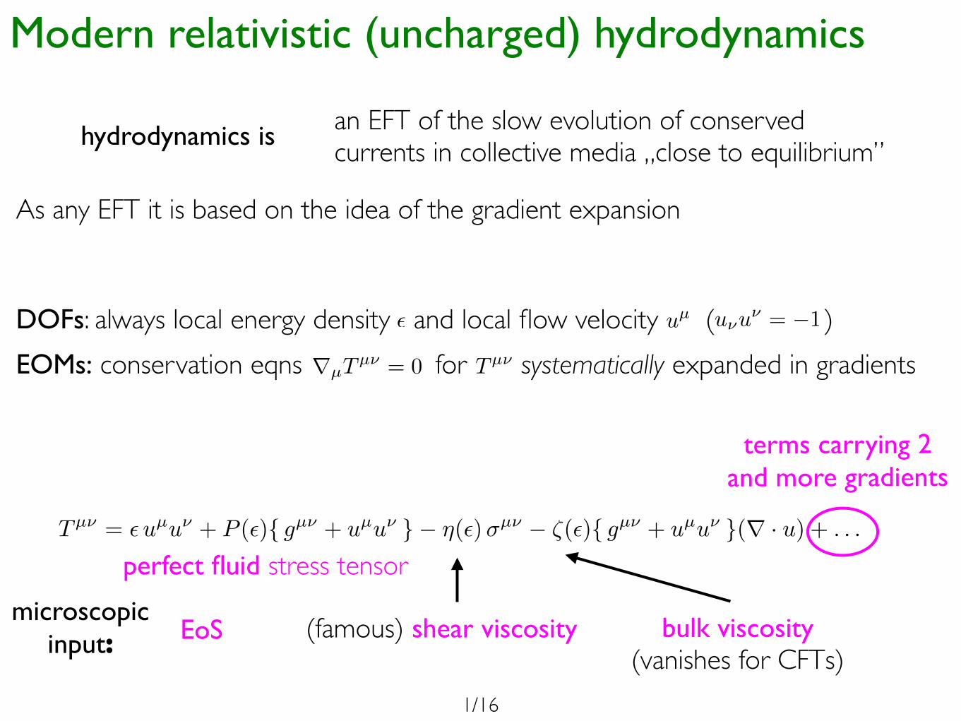
an EFT of the slow evolution of conserved currents in collective media „close to equilibrium”hydrodynamics is

As any EFT it is based on the idea of the gradient expansion

DOFs: always local energy density and local flow velocity ( )EOMs: conservation eqns for systematically expanded in gradients

✏ uµ u⌫u⌫ = �1

rµTµ⌫ = 0

Tµ⌫ = ✏uµu⌫ + P (✏){ gµ⌫ + uµu⌫ }� ⌘(✏)�µ⌫ � ⇣(✏){ gµ⌫ + uµu⌫ }(r · u) + . . .

Tµ⌫

perfect fluid stress tensor

(famous) shear viscosity bulk viscosity(vanishes for CFTs)

microscopicinput: EoS

terms carrying 2and more gradients

1/16

Applicability of hydrodynamics

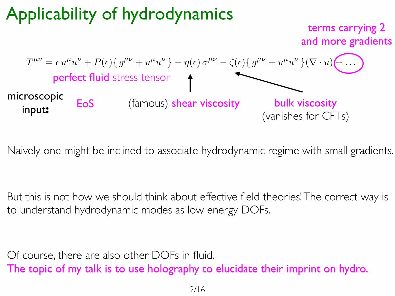
Tµ⌫ = ✏uµu⌫ + P (✏){ gµ⌫ + uµu⌫ }� ⌘(✏)�µ⌫ � ⇣(✏){ gµ⌫ + uµu⌫ }(r · u) + . . .

perfect fluid stress tensor

(famous) shear viscosity bulk viscosity(vanishes for CFTs)

microscopicinput: EoS

terms carrying 2and more gradients

Naively one might be inclined to associate hydrodynamic regime with small gradients.

But this is not how we should think about effective field theories! The correct way is to understand hydrodynamic modes as low energy DOFs.

Of course, there are also other DOFs in fluid.The topic of my talk is to use holography to elucidate their imprint on hydro.

2/16

Holographic plasmasand their degrees of freedom

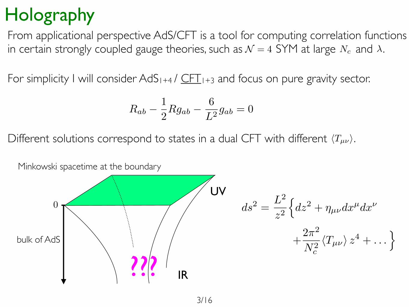
HolographyFrom applicational perspective AdS/CFT is a tool for computing correlation functions in certain strongly coupled gauge theories, such as SYM at large and . N = 4

For simplicity I will consider AdS1+4 / CFT1+3 and focus on pure gravity sector.

Nc �

0

Minkowski spacetime at the boundary

bulk of AdS

Rab �1

2Rgab �

6

L2gab = 0

UV

IR

Different solutions correspond to states in a dual CFT with different . hTµ⌫i

???

ds

2 =L

2

z

2

ndz

2 + ⌘µ⌫dxµdx

⌫

+2⇡2

N2c

hTµ⌫i z4 + . . .o

3/16

Excitations of strongly coupled plasmas Kovtun & Starinets [hep-th/0506184]

Tµ⌫ =18⇡2N2

c T 4 diag (3, 1, 1, 1)µ⌫ +�Tµ⌫

(⇠ e�i!(k) t+i

~

k·~x)

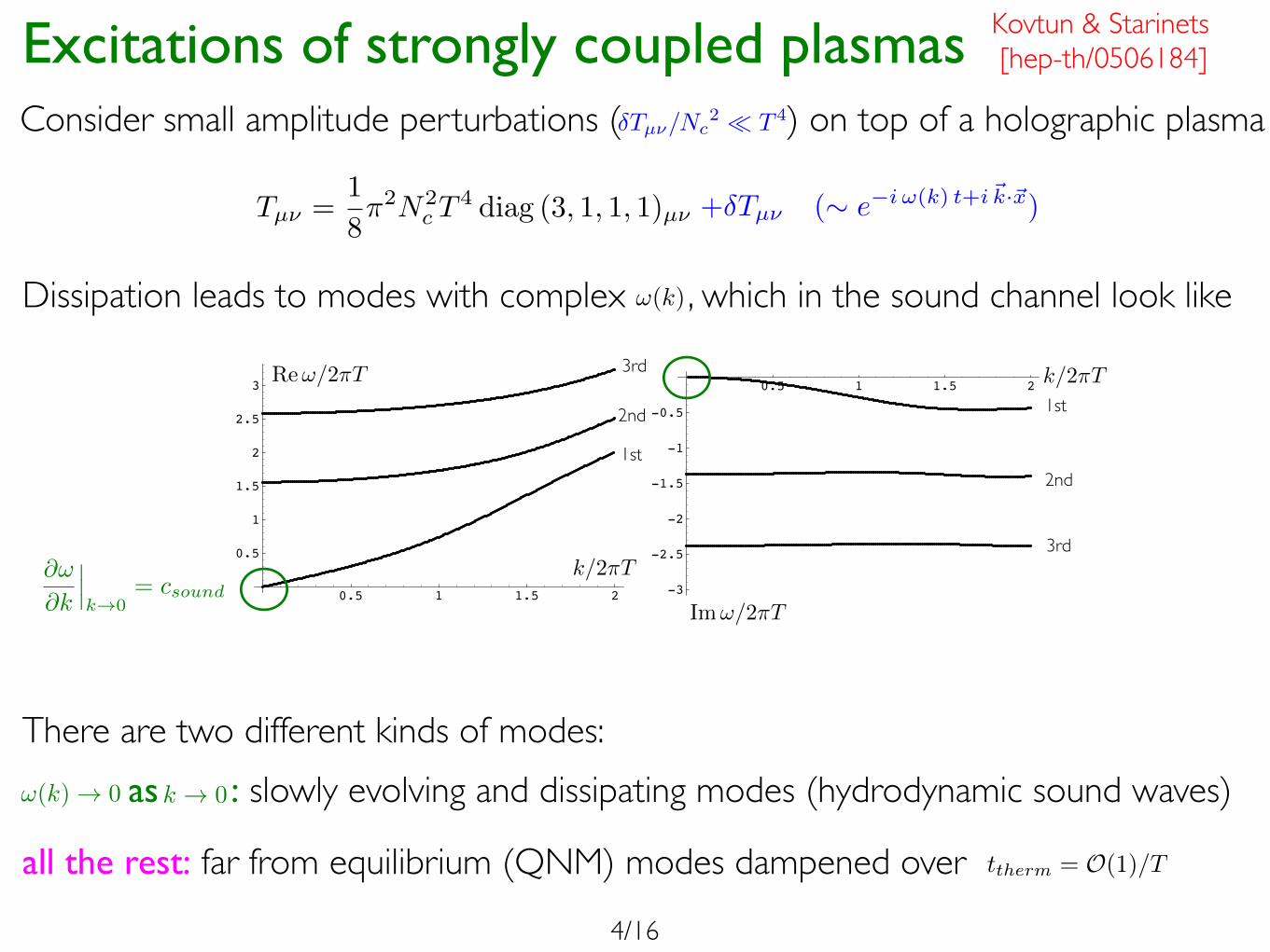
Consider small amplitude perturbations ( ) on top of a holographic plasma�Tµ⌫/Nc2 ⌧ T 4

Dissipation leads to modes with complex , which in the sound channel look like!(k)

0.5 1 1.5 2

0.5

1

1.5

2

2.5

3 Re 0.5 1 1.5 2

-3

-2.5

-2

-1.5

-1

-0.5

Im

Figure 6: Real and imaginary parts of three lowest quasinormal frequencies as function of spatialmomentum. The curves for which !0 as !0 correspond to hydrodynamic sound mode in the dualfinite temperature N=4 SYM theory.

behavior of the lowest (hydrodynamic) frequency which is absent for E! and Z3. For Ez and

Z1, hydrodynamic frequencies are purely imaginary (given by Eqs. (4.16) and (4.32) for small

! and q), and presumably move o! to infinity as q becomes large. For Z2, the hydrodynamic

frequency has both real and imaginary parts (given by Eq. (4.44) for small ! and q), and

eventually (for large q) becomes indistinguishable in the tower of other eigenfrequencies. As an

example, dispersion relations for the three lowest quasinormal frequencies in the sound channel

(including the one of the sound wave) are shown in Fig. 6. The tables below give numerical

values of quasinormal frequencies for = 1. Only non-hydrodynamic frequencies are shown

in the tables. The position of hydrodynamic frequencies at = 1 is = "3.250637i for the

R-charge di!usive mode, = "0.598066i for the shear mode, and = ±0.741420"0.286280i

for the sound mode. The numerical values of the lowest five (non-hydrodynamic) quasinormal

frequencies for electromagnetic perturbations are:

Transverse channel Di!usive channel

n Re Im Re Im

1 ±1.547187 "0.849723 ±1.147831 "0.559204

2 ±2.398903 "1.874343 ±1.910006 "1.758065

3 ±3.323229 "2.894901 ±2.903293 "2.891681

4 ±4.276431 "3.909583 ±3.928555 "3.943386

5 ±5.244062 "4.920336 ±4.946818 "4.965186

and for gravitational perturbations are:

Scalar channel Shear channel Sound channel

n Re Im Re Im Re Im

1 ±1.954331 "1.267327 ±1.759116 "1.291594 ±1.733511 "1.343008

2 ±2.880263 "2.297957 ±2.733081 "2.330405 ±2.705540 "2.357062

3 ±3.836632 "3.314907 ±3.715933 "3.345343 ±3.689392 "3.363863

4 ±4.807392 "4.325871 ±4.703643 "4.353487 ±4.678736 "4.367981

5 ±5.786182 "5.333622 ±5.694472 "5.358205 ±5.671091 "5.370784

– 26 –

Im!/2⇡T

Re!/2⇡T

k/2⇡T

k/2⇡T

1st

2nd

3rd

1st

2nd

3rd

!(k) ! 0 as : slowly evolving and dissipating modes (hydrodynamic sound waves)k ! 0

all the rest: far from equilibrium (QNM) modes dampened over

@!

@k

���k!0

= csound

ttherm = O(1)/T

There are two different kinds of modes:

4/16

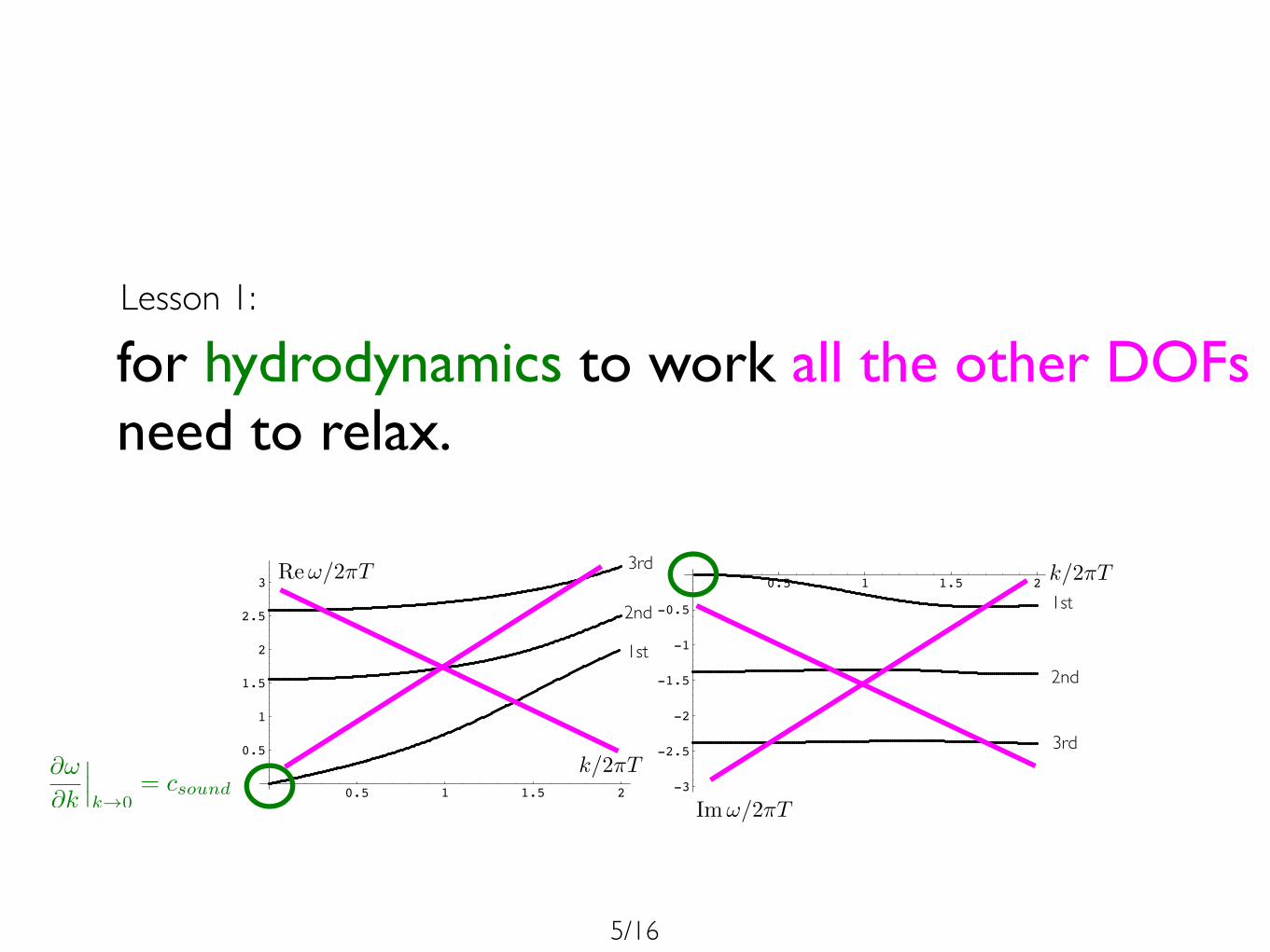
for hydrodynamics to work all the other DOFsneed to relax.

Lesson 1:

0.5 1 1.5 2

0.5

1

1.5

2

2.5

3 Re 0.5 1 1.5 2

-3

-2.5

-2

-1.5

-1

-0.5

Im

Figure 6: Real and imaginary parts of three lowest quasinormal frequencies as function of spatialmomentum. The curves for which !0 as !0 correspond to hydrodynamic sound mode in the dualfinite temperature N=4 SYM theory.

behavior of the lowest (hydrodynamic) frequency which is absent for E! and Z3. For Ez and

Z1, hydrodynamic frequencies are purely imaginary (given by Eqs. (4.16) and (4.32) for small

! and q), and presumably move o! to infinity as q becomes large. For Z2, the hydrodynamic

frequency has both real and imaginary parts (given by Eq. (4.44) for small ! and q), and

eventually (for large q) becomes indistinguishable in the tower of other eigenfrequencies. As an

example, dispersion relations for the three lowest quasinormal frequencies in the sound channel

(including the one of the sound wave) are shown in Fig. 6. The tables below give numerical

values of quasinormal frequencies for = 1. Only non-hydrodynamic frequencies are shown

in the tables. The position of hydrodynamic frequencies at = 1 is = "3.250637i for the

R-charge di!usive mode, = "0.598066i for the shear mode, and = ±0.741420"0.286280i

for the sound mode. The numerical values of the lowest five (non-hydrodynamic) quasinormal

frequencies for electromagnetic perturbations are:

Transverse channel Di!usive channel

n Re Im Re Im

1 ±1.547187 "0.849723 ±1.147831 "0.559204

2 ±2.398903 "1.874343 ±1.910006 "1.758065

3 ±3.323229 "2.894901 ±2.903293 "2.891681

4 ±4.276431 "3.909583 ±3.928555 "3.943386

5 ±5.244062 "4.920336 ±4.946818 "4.965186

and for gravitational perturbations are:

Scalar channel Shear channel Sound channel

n Re Im Re Im Re Im

1 ±1.954331 "1.267327 ±1.759116 "1.291594 ±1.733511 "1.343008

2 ±2.880263 "2.297957 ±2.733081 "2.330405 ±2.705540 "2.357062

3 ±3.836632 "3.314907 ±3.715933 "3.345343 ±3.689392 "3.363863

4 ±4.807392 "4.325871 ±4.703643 "4.353487 ±4.678736 "4.367981

5 ±5.786182 "5.333622 ±5.694472 "5.358205 ±5.671091 "5.370784

– 26 –

Im!/2⇡T

Re!/2⇡T

k/2⇡T

k/2⇡T

1st

2nd

3rd

1st

2nd

3rd@!

@k

���k!0

= csound

5/16

0.5 1 1.5 2

0.5

1

1.5

2

2.5

3 Re 0.5 1 1.5 2

-3

-2.5

-2

-1.5

-1

-0.5

Im

Figure 6: Real and imaginary parts of three lowest quasinormal frequencies as function of spatialmomentum. The curves for which !0 as !0 correspond to hydrodynamic sound mode in the dualfinite temperature N=4 SYM theory.

behavior of the lowest (hydrodynamic) frequency which is absent for E! and Z3. For Ez and

Z1, hydrodynamic frequencies are purely imaginary (given by Eqs. (4.16) and (4.32) for small

! and q), and presumably move o! to infinity as q becomes large. For Z2, the hydrodynamic

frequency has both real and imaginary parts (given by Eq. (4.44) for small ! and q), and

eventually (for large q) becomes indistinguishable in the tower of other eigenfrequencies. As an

example, dispersion relations for the three lowest quasinormal frequencies in the sound channel

(including the one of the sound wave) are shown in Fig. 6. The tables below give numerical

values of quasinormal frequencies for = 1. Only non-hydrodynamic frequencies are shown

in the tables. The position of hydrodynamic frequencies at = 1 is = "3.250637i for the

R-charge di!usive mode, = "0.598066i for the shear mode, and = ±0.741420"0.286280i

for the sound mode. The numerical values of the lowest five (non-hydrodynamic) quasinormal

frequencies for electromagnetic perturbations are:

Transverse channel Di!usive channel

n Re Im Re Im

1 ±1.547187 "0.849723 ±1.147831 "0.559204

2 ±2.398903 "1.874343 ±1.910006 "1.758065

3 ±3.323229 "2.894901 ±2.903293 "2.891681

4 ±4.276431 "3.909583 ±3.928555 "3.943386

5 ±5.244062 "4.920336 ±4.946818 "4.965186

and for gravitational perturbations are:

Scalar channel Shear channel Sound channel

n Re Im Re Im Re Im

1 ±1.954331 "1.267327 ±1.759116 "1.291594 ±1.733511 "1.343008

2 ±2.880263 "2.297957 ±2.733081 "2.330405 ±2.705540 "2.357062

3 ±3.836632 "3.314907 ±3.715933 "3.345343 ±3.689392 "3.363863

4 ±4.807392 "4.325871 ±4.703643 "4.353487 ±4.678736 "4.367981

5 ±5.786182 "5.333622 ±5.694472 "5.358205 ±5.671091 "5.370784

– 26 –

Im!/2⇡T

Re!/2⇡T

k/2⇡T

k/2⇡T

1st

2nd

3rd

1st

2nd

3rd@!

@k

���k!0

= csound

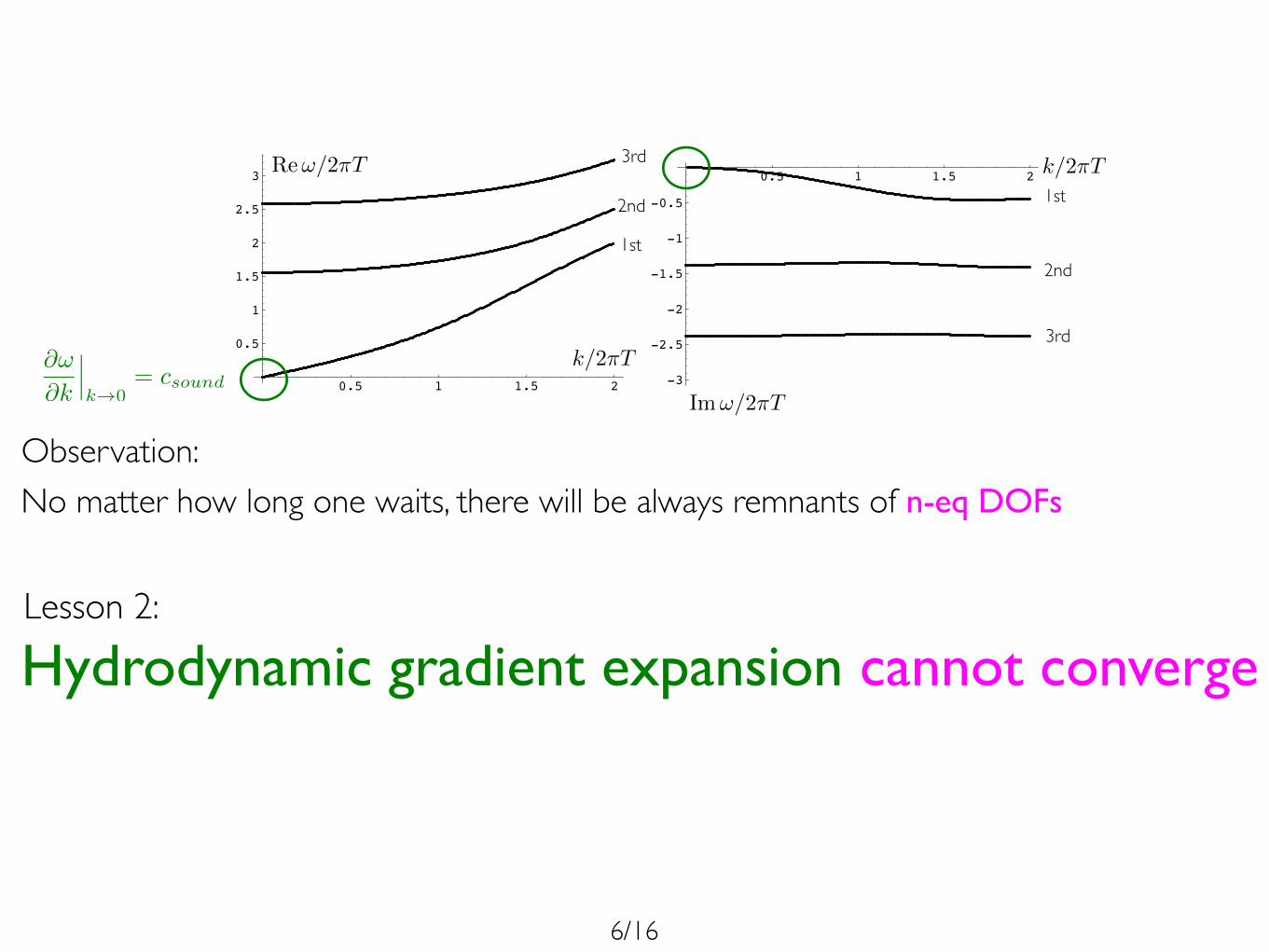
Observation:No matter how long one waits, there will be always remnants of n-eq DOFs

Hydrodynamic gradient expansion cannot convergeLesson 2:

6/16

Dynamical model

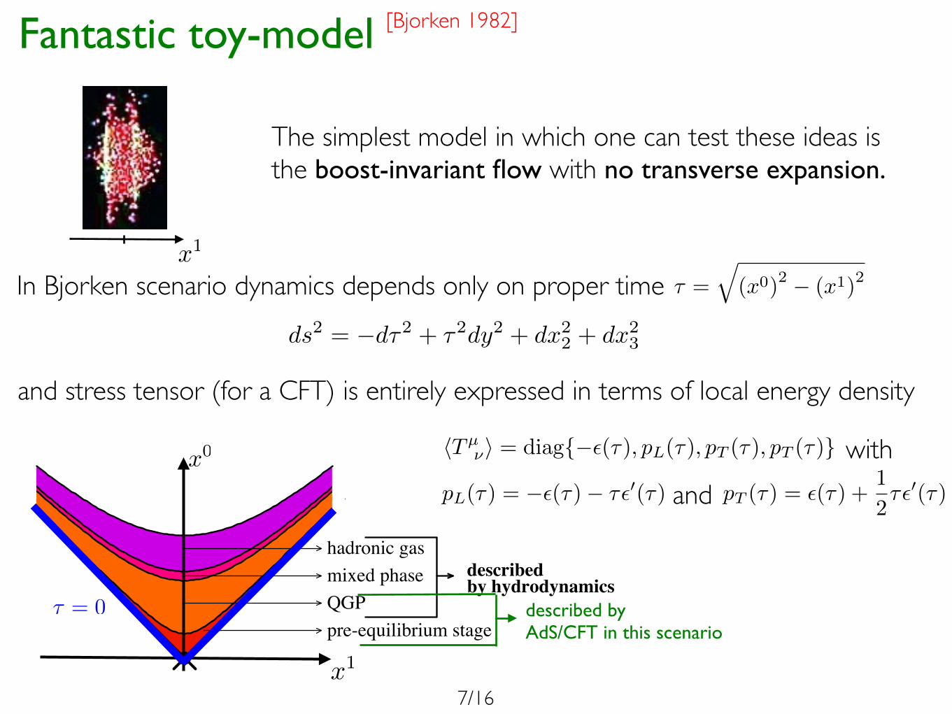
Fantastic toy-model

x

0

x

1

x

1

The simplest model in which one can test these ideas isthe boost-invariant flow with no transverse expansion.

In Bjorken scenario dynamics depends only on proper time

[Bjorken 1982]

pre-equilibrium stageQGPmixed phasehadronic gas

describedby hydrodynamics

Figure 1: Description of QGP formation in heavy ion collisions. The kinematic landscape isdefined by ! =

!

(x0)2 ! (x3)2 ; y = 12 log x

0+x3

x0!x3 ; x"={x1, x2} , where the coordinates along thelight-cone are x0 ± x1, the transverse ones are {x1, x2} and ! is the proper time, y the “space-timerapidity”.

[3]. The hydrodynamic regime has to last long enough and start soon enough after the

collision in order to explain the observed collective e!ects. Moreover, the smallness of the

viscosity which can be extracted from hydrodynamical simulations describing the data leads

to an almost-perfect fluid behaviour of the QGP, and thus to a short mean-free path inside

the fluid. Putting together these experimental inputs, and in order to go beyond a mererly

phenomenological description, it appears to be theoretically necessary to investigate as

much as possible the properties of a strongly-coupled Quantum-Chromodynamic plasma.

In the absence of nonperturbative methods applicable to real-time dynamics of strongly

coupled Quantum Chromodynamic (QCD) plasma, one is led to consider similar problems

from the point-of-view of the AdS/CFT correspondence, that is looking for the charac-

teristics of plasma in a gauge theory for which the AdS/CFT correspondence takes its

simplest form – the N = 4 supersymmetric Yang-Mills theory [4] which posseses a known

and tractable gravity dual.

Although the N = 4 gauge theory is supersymmetric and conformal and thus quite

di!erent from QCD at zero temperature, both supersymmetry and scale-invariance are

broken explicitly at finite temperature and we may expect qualitative similarities with

QCD plasma for a range of temperatures above the QCD deconfinement phase transition1.

Indeed, the gauge/gravity dual calculation [5] showing, in a static setting, that the

viscosity over entropy ratio "/s is very small (equal to 1/4#) and even suggesting a universal

lower bound, is in qualitative agreement with hydrodynamic simulations of QCD plasma

and was a poweful incentive to explore further the AdS/CFT duality approach.

In order to go beyond static calculations, one has to adapt the dual AdS/CFT approach

to the relativistic kinematic framework of heavy-ion reactions, where two ultra-relativistic

heavy nuclei collide and form an expanding medium, see Fig.1. It is convenient, initially,

1There exist more refined versions of the AdS/CFT correspondence which may have more features in

common with QCD, however the gravity backgrounds are much more complicated and we will not consider

them here.

– 2 –

described by AdS/CFT in this scenario

and stress tensor (for a CFT) is entirely expressed in terms of local energy density

with

⌧ = 0

� =q

(x0)2 � (x1)2

and pT (⇥) = �(⇥) +1

2⇥�0(⇥)pL(⇥) = ��(⇥)� ⇥�0(⇥)

hTµ⌫i = diag{�✏(⌧), pL(⌧), pT (⌧), pT (⌧)}

ds

2 = �d⌧

2 + ⌧

2dy

2 + dx

22 + dx

23

7/16

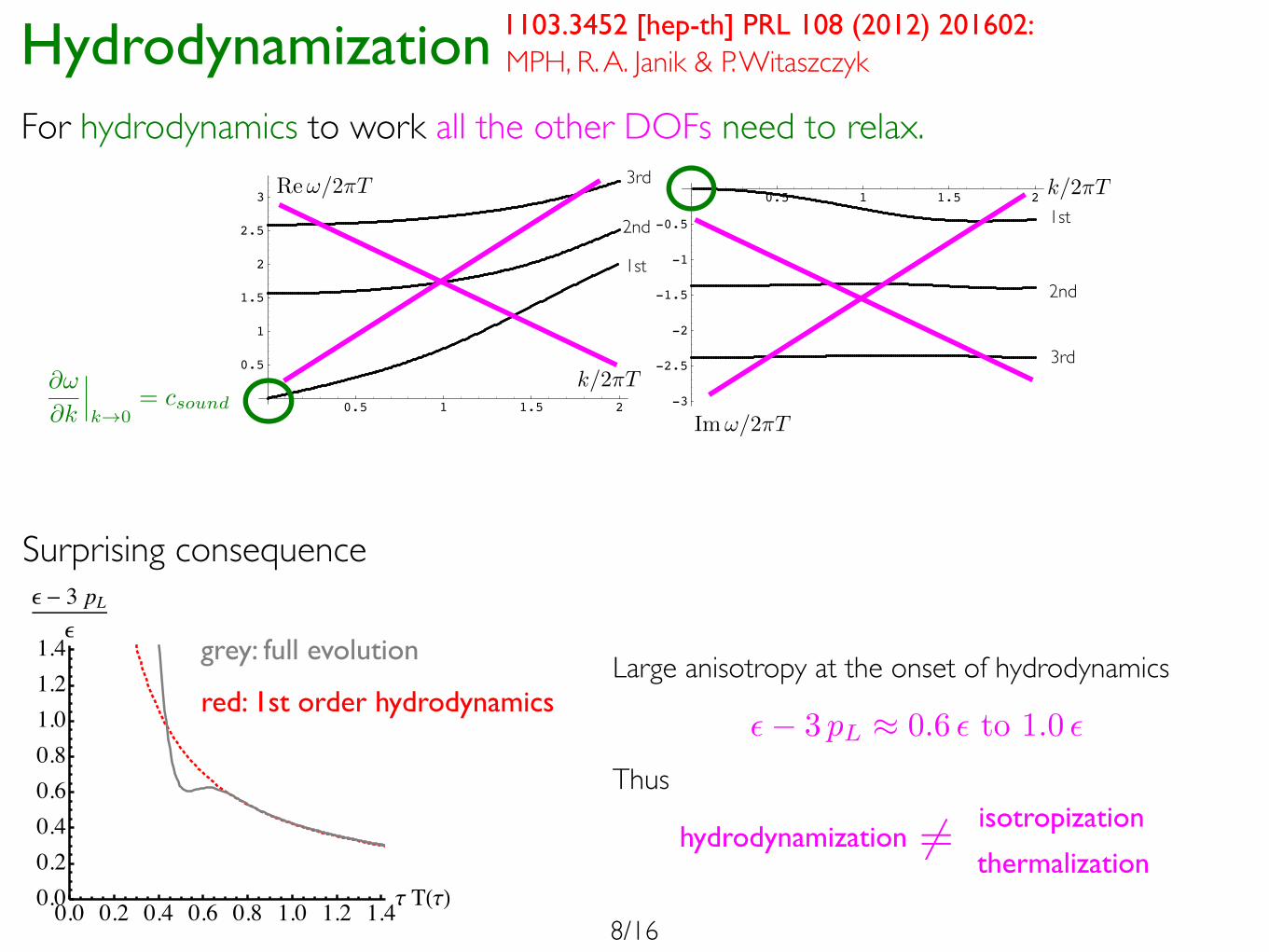
Hydrodynamization

6=

✏� 3 pL ⇡ 0.6 ✏ to 1.0 ✏

0.0 0.2 0.4 0.6 0.8 1.0 1.2 1.4t THtL0.00.20.40.60.81.01.21.4

e - 3 pLe

grey: full evolution

red: 1st order hydrodynamicsLarge anisotropy at the onset of hydrodynamics

Thus

hydrodynamization

0.5 1 1.5 2

0.5

1

1.5

2

2.5

3 Re 0.5 1 1.5 2

-3

-2.5

-2

-1.5

-1

-0.5

Im

Figure 6: Real and imaginary parts of three lowest quasinormal frequencies as function of spatialmomentum. The curves for which !0 as !0 correspond to hydrodynamic sound mode in the dualfinite temperature N=4 SYM theory.

behavior of the lowest (hydrodynamic) frequency which is absent for E! and Z3. For Ez and

Z1, hydrodynamic frequencies are purely imaginary (given by Eqs. (4.16) and (4.32) for small

! and q), and presumably move o! to infinity as q becomes large. For Z2, the hydrodynamic

frequency has both real and imaginary parts (given by Eq. (4.44) for small ! and q), and

eventually (for large q) becomes indistinguishable in the tower of other eigenfrequencies. As an

example, dispersion relations for the three lowest quasinormal frequencies in the sound channel

(including the one of the sound wave) are shown in Fig. 6. The tables below give numerical

values of quasinormal frequencies for = 1. Only non-hydrodynamic frequencies are shown

in the tables. The position of hydrodynamic frequencies at = 1 is = "3.250637i for the

R-charge di!usive mode, = "0.598066i for the shear mode, and = ±0.741420"0.286280i

for the sound mode. The numerical values of the lowest five (non-hydrodynamic) quasinormal

frequencies for electromagnetic perturbations are:

Transverse channel Di!usive channel

n Re Im Re Im

1 ±1.547187 "0.849723 ±1.147831 "0.559204

2 ±2.398903 "1.874343 ±1.910006 "1.758065

3 ±3.323229 "2.894901 ±2.903293 "2.891681

4 ±4.276431 "3.909583 ±3.928555 "3.943386

5 ±5.244062 "4.920336 ±4.946818 "4.965186

and for gravitational perturbations are:

Scalar channel Shear channel Sound channel

n Re Im Re Im Re Im

1 ±1.954331 "1.267327 ±1.759116 "1.291594 ±1.733511 "1.343008

2 ±2.880263 "2.297957 ±2.733081 "2.330405 ±2.705540 "2.357062

3 ±3.836632 "3.314907 ±3.715933 "3.345343 ±3.689392 "3.363863

4 ±4.807392 "4.325871 ±4.703643 "4.353487 ±4.678736 "4.367981

5 ±5.786182 "5.333622 ±5.694472 "5.358205 ±5.671091 "5.370784

– 26 –

Im!/2⇡T

Re!/2⇡T

k/2⇡T

k/2⇡T

1st

2nd

3rd

1st

2nd

3rd@!

@k

���k!0

= csound

For hydrodynamics to work all the other DOFs need to relax.

Surprising consequence

thermalization

isotropization

MPH, R. A. Janik & P. Witaszczyk1103.3452 [hep-th] PRL 108 (2012) 201602:

8/16

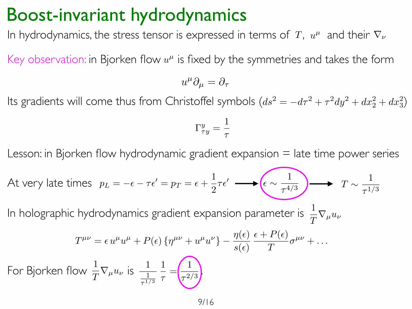
Boost-invariant hydrodynamicsIn hydrodynamics, the stress tensor is expressed in terms of , and their T uµ r⌫

Key observation: in Bjorken flow is fixed by the symmetries and takes the form

uµ@µ = @⌧

uµ

Its gradients will come thus from Christoffel symbols ( )ds

2 = �d⌧

2 + ⌧

2dy

2 + dx

22 + dx

23

Lesson: in Bjorken flow hydrodynamic gradient expansion = late time power series

At very late times pL = �✏� ⌧✏0 = pT = ✏+1

2⌧✏0 ✏ ⇠ 1

⌧4/3T ⇠ 1

⌧1/3

�y⌧y =

1

⌧

In holographic hydrodynamics gradient expansion parameter is

Tµ⌫ = ✏uµuµ + P (✏) {⌘µ⌫ + uµu⌫}� ⌘(✏)

s(✏)

✏+ P (✏)

T�µ⌫ + . . .

1

Trµu⌫

For Bjorken flow is .1

Trµu⌫

11

⌧1/3

1

⌧=

1

⌧2/3

9/16

High order hydrodynamics

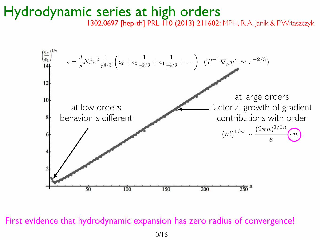
Hydrodynamic series at high ordersMPH, R. A. Janik & P. Witaszczyk1302.0697 [hep-th] PRL 110 (2013) 211602:

at large ordersfactorial growth of gradient contributions with order

T 00 = ✏(⌧) ⇠1X

n=2

✏n(⌧�2/3)n (T�1rµu

⌫ ⇠ ⌧�2/3)

First evidence that hydrodynamic expansion has zero radius of convergence!

at low ordersbehavior is different

2

longitudinal direction. This symmetry can be made man-ifest upon passing to curvilinear proper time ⌧ - rapidityy coordinates related to the lab frame time x

0 and posi-tion along the expansion axis x1 via

x

0 = ⌧ cosh y and x

1 = ⌧ sinh y. (1)

In the case of (3+1)-dimensional conformal field theoryplasma, the most general stress tensor obeying the sym-metries of the problem in coordinates (⌧, y, x1

, x

2) reads

T

µ⌫ = diag(�✏, pL, pT , pT )

µ⌫ , (2)

where the energy density ✏ is a function of proper timeonly and the longitudinal pL and transverse pT pressuresare fully expressed in terms of the energy density [9]

pL = �✏� ⌧ ✏

0 and pT = ✏+1

2⌧ ✏

0. (3)

Note that, in the proper time - rapidity coordinates (1),there is no momentum flow in the stress tensor (2) andso the flow velocity is trivial and takes the form u =@⌧ . Hydrodynamic constituent relations lead, then, togradient expanded energy density of the form

✏ =3

8N

2

c ⇡2

1

⌧

4/3

✓✏

2

+ ✏

3

1

⌧

2/3+ ✏

4

1

⌧

4/3+ . . .

◆, (4)

where the choice of ✏2

sets an overall energy scale, in par-ticular for the quasinormal frequencies (7) and 9). Theprefactor was chosen to match the N = 4 super Yang-Mills theory at large-Nc and strong coupling. In the fol-lowing, we choose the units by setting ✏

2

= ⇡

�4.Large-⌧ expansion of the energy density in powers of

⌧

�2/3, as in (4), is equivalent to the hydrodynamic gra-dient expansion and arises from expressing gradients ofvelocity (rµu⌫ ⇠ ⌧

�1) in units of the e↵ective tempera-ture (T ⇠ ✏

1/4 ⇠ ⌧

�1/3). The value of the coe�cient ✏

3

is related to the shear viscosity ⌘, whereas ✏

4

is a sumof two transport coe�cients: relaxation time ⌧

⇧

and theso-called �

1

[10]. Higher order contributions to the en-ergy density are expected to be linear combinations of sofar unidentified transport coe�cients. Note also that theexpansion (4) is sensitive to both linear and nonlineargradient terms.

As explained in [11, 12] (see also Supplemental ma-terial), higher order contributions to the energy density(4) can be obtained by solving Einstein’s equations witha negative cosmological constant for the metric ansatz ofthe form

ds

2 = 2d⌧dr�Ad⌧

2+⌃2

e

�2Bdy

2+⌃2

e

B(dx2

1

+dx

2

2

), (5)

where the warp factors A, ⌃ and B are functions of rand ⌧ constructed in the gradient expansion as requiredby the fluid-gravity duality. At leading order, the warpfactors are that of a locally boosted black brane and this

solution gets systematically corrected in ⌧

�2/3 expansion,as is the case with the energy density in the dual fieldtheory (4).The background expanded in ⌧

�2/3 around a locallyboosted black brane is slowly evolving and captures onlyhydrodynamic degrees of freedom. One can, in ad-dition, consider the incorporation of nonhydrodynamic(fast evolving) degrees of freedom by linearizing Ein-stein’s equations on top of the hydrodynamic solution,i.e. B = B

hydro

+ �B, and similarly for A and ⌃, andlooking for �B corresponding to (at very large time) theexponentially decaying contribution to the stress tensordepending only on ⌧ . For the static background analo-gous calculation would lead to the spectrum of nonhydro-dynamic quasinormal modes carrying zero momentum,which is known to be the same as the spectrum of zeromomentum quasinormal modes for the massless scalarfield [13].In the leading order of the gradient expansion, the re-

sulting modes, on the gravity side, indeed essentially re-duce to the scalar quasinormal modes but obtain an ad-ditional factor of 3

2

and are damped exponentially in ⌧

2

3

[14]. Upon including viscous correction, the modes ob-tain a further nontrivial powerlike preexponential factor

�✏ ⇠ ⌧

↵qnm exp (�i

3

2!qnm ⌧

2/3). (6)

Explicit gravity calculation for the lowest mode yield

!qnm = 3.1195�2.7467, ↵qnm = �1.5422+0.5199 i. (7)

The frequency !qnm agrees with the frequency of thelowest nonhydrodynamic scalar quasinormal mode andwas calculated before in [14], whereas the prediction of↵qnm is a new result specific to the dissipative modifi-cations of the expanding black hole geometry (see theSupplemental Material for further details). In the fol-lowing, we will be able to reproduce numerically (7) justfrom the large order behavior of the hydrodynamic series.Large order behavior of hydrodynamic energy

density. Numerical implementation of the methods out-lined in [11, 12] allow for e�cient calculation of hydrody-namic series given by (4), up to a very large order, sinceone is e↵ectively solving a set of linear ODE’s (comingfrom Einstein’s equations) at each order. Using spectralmethods we iteratively solved these equations in the largetime expansion reconstructing the energy density up tothe order 240, i.e. up to the term ✏

242

in (4). To the bestof our knowledge this is the first approach allowing us toaccess information about the large order behavior of thehydrodynamic series in any physical system or model.As a way of monitoring the accuracy of our procedures

we compared normalized values of evaluated Einstein’sequations at each order of the ⌧

�2/3 expansion to theratio of coe�cients of gradient-expanded energy densityto gradient expanded warp factors. This ensures thatour results for the energy density are reliable. We also

(n!)1/n ⇠ (2⇡n)1/2n

e· n

10/16

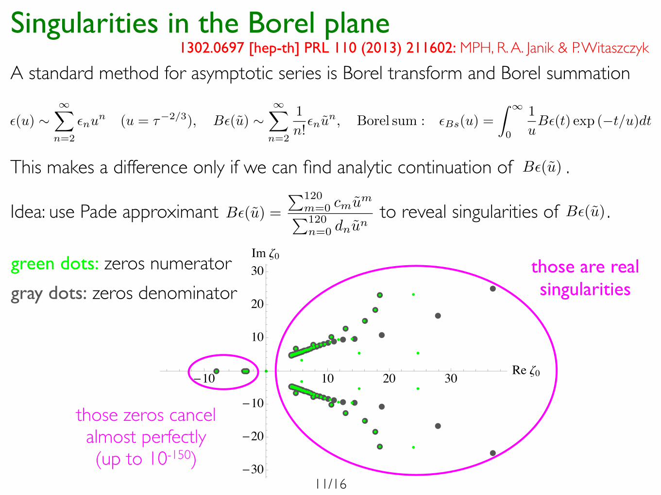
A standard method for asymptotic series is Borel transform and Borel summationMPH, R. A. Janik & P. Witaszczyk

Singularities in the Borel plane

✏(u) ⇠1X

n=2

✏nun

(u = ⌧�2/3), B✏(u) ⇠

1X

n=2

1

n!✏nu

n, Borel sum : ✏Bs(u) =

Z 1

0

1

uB✏(t) exp (�t/u)dt

1302.0697 [hep-th] PRL 110 (2013) 211602:

This makes a difference only if we can find analytic continuation of .B✏(u)

Idea: use Pade approximant to reveal singularities of .B✏(u) =

P120m=0 cmum

P120n=0 dnu

nB✏(u)

-10 10 20 30 Re z0

-30

-20

-10

10

20

30Im z0green dots: zeros numerator

gray dots: zeros denominator

those zeros cancel almost perfectly(up to 10-150)

those are realsingularities

11/16

Hydrodynamic instantons andhydrodynamic gradient expansion

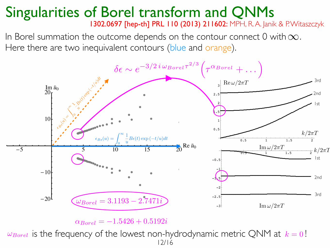
In Borel summation the outcome depends on the contour connect 0 with .Here there are two inequivalent contours (blue and orange).

MPH, R. A. Janik & P. WitaszczykSingularities of Borel transform and QNMs

is the frequency of the lowest non-hydrodynamic metric QNM at !

0.5 1 1.5 2

0.5

1

1.5

2

2.5

3 Re 0.5 1 1.5 2

-3

-2.5

-2

-1.5

-1

-0.5

Im

Figure 6: Real and imaginary parts of three lowest quasinormal frequencies as function of spatialmomentum. The curves for which !0 as !0 correspond to hydrodynamic sound mode in the dualfinite temperature N=4 SYM theory.

behavior of the lowest (hydrodynamic) frequency which is absent for E! and Z3. For Ez and

Z1, hydrodynamic frequencies are purely imaginary (given by Eqs. (4.16) and (4.32) for small

! and q), and presumably move o! to infinity as q becomes large. For Z2, the hydrodynamic

frequency has both real and imaginary parts (given by Eq. (4.44) for small ! and q), and

eventually (for large q) becomes indistinguishable in the tower of other eigenfrequencies. As an

example, dispersion relations for the three lowest quasinormal frequencies in the sound channel

(including the one of the sound wave) are shown in Fig. 6. The tables below give numerical

values of quasinormal frequencies for = 1. Only non-hydrodynamic frequencies are shown

in the tables. The position of hydrodynamic frequencies at = 1 is = "3.250637i for the

R-charge di!usive mode, = "0.598066i for the shear mode, and = ±0.741420"0.286280i

for the sound mode. The numerical values of the lowest five (non-hydrodynamic) quasinormal

frequencies for electromagnetic perturbations are:

Transverse channel Di!usive channel

n Re Im Re Im

1 ±1.547187 "0.849723 ±1.147831 "0.559204

2 ±2.398903 "1.874343 ±1.910006 "1.758065

3 ±3.323229 "2.894901 ±2.903293 "2.891681

4 ±4.276431 "3.909583 ±3.928555 "3.943386

5 ±5.244062 "4.920336 ±4.946818 "4.965186

and for gravitational perturbations are:

Scalar channel Shear channel Sound channel

n Re Im Re Im Re Im

1 ±1.954331 "1.267327 ±1.759116 "1.291594 ±1.733511 "1.343008

2 ±2.880263 "2.297957 ±2.733081 "2.330405 ±2.705540 "2.357062

3 ±3.836632 "3.314907 ±3.715933 "3.345343 ±3.689392 "3.363863

4 ±4.807392 "4.325871 ±4.703643 "4.353487 ±4.678736 "4.367981

5 ±5.786182 "5.333622 ±5.694472 "5.358205 ±5.671091 "5.370784

– 26 –

Im!/2⇡T

Re!/2⇡T

k/2⇡T

k/2⇡T

1st

2nd 1st

2nd

3rd

0.5 1 1.5 2

0.5

1

1.5

2

2.5

3 Re 0.5 1 1.5 2

-3

-2.5

-2

-1.5

-1

-0.5

Im

Figure 6: Real and imaginary parts of three lowest quasinormal frequencies as function of spatialmomentum. The curves for which !0 as !0 correspond to hydrodynamic sound mode in the dualfinite temperature N=4 SYM theory.

behavior of the lowest (hydrodynamic) frequency which is absent for E! and Z3. For Ez and

Z1, hydrodynamic frequencies are purely imaginary (given by Eqs. (4.16) and (4.32) for small

! and q), and presumably move o! to infinity as q becomes large. For Z2, the hydrodynamic

frequency has both real and imaginary parts (given by Eq. (4.44) for small ! and q), and

eventually (for large q) becomes indistinguishable in the tower of other eigenfrequencies. As an

example, dispersion relations for the three lowest quasinormal frequencies in the sound channel

(including the one of the sound wave) are shown in Fig. 6. The tables below give numerical

values of quasinormal frequencies for = 1. Only non-hydrodynamic frequencies are shown

in the tables. The position of hydrodynamic frequencies at = 1 is = "3.250637i for the

R-charge di!usive mode, = "0.598066i for the shear mode, and = ±0.741420"0.286280i

for the sound mode. The numerical values of the lowest five (non-hydrodynamic) quasinormal

frequencies for electromagnetic perturbations are:

Transverse channel Di!usive channel

n Re Im Re Im

1 ±1.547187 "0.849723 ±1.147831 "0.559204

2 ±2.398903 "1.874343 ±1.910006 "1.758065

3 ±3.323229 "2.894901 ±2.903293 "2.891681

4 ±4.276431 "3.909583 ±3.928555 "3.943386

5 ±5.244062 "4.920336 ±4.946818 "4.965186

and for gravitational perturbations are:

Scalar channel Shear channel Sound channel

n Re Im Re Im Re Im

1 ±1.954331 "1.267327 ±1.759116 "1.291594 ±1.733511 "1.343008

2 ±2.880263 "2.297957 ±2.733081 "2.330405 ±2.705540 "2.357062

3 ±3.836632 "3.314907 ±3.715933 "3.345343 ±3.689392 "3.363863

4 ±4.807392 "4.325871 ±4.703643 "4.353487 ±4.678736 "4.367981

5 ±5.786182 "5.333622 ±5.694472 "5.358205 ±5.671091 "5.370784

– 26 –

Im!/2⇡T

Re!/2⇡T

k/2⇡T

1st

2nd

3rd

-5 5 10 15 20Re ué0

-20

-10

10

20Im ué0

✏Bs(

u)=

Z 1

01

uB✏(t)e

x

p

(

�t/u)

dt

✏Bs(u) =

Z 1

0

1

uB✏(t) exp (�t/u)dt

1302.0697 [hep-th] PRL 110 (2013) 211602:

12/16

1

�✏ ⇠ e�3/2 i!Borel

⌧2/3⇣⌧↵Borel + . . .

⌘

!Borel

= 3.1193� 2.7471i

↵Borel

= �1.5426 + 0.5192i

!Borel

k = 0

MPH, R. A. Janik & P. WitaszczykSlow and fast modes

1302.0697 [hep-th] PRL 110 (2013) 211602:

13/16

�✏ ⇠ e�3/2 i!Borel

⌧2/3⇣⌧↵Borel + . . .

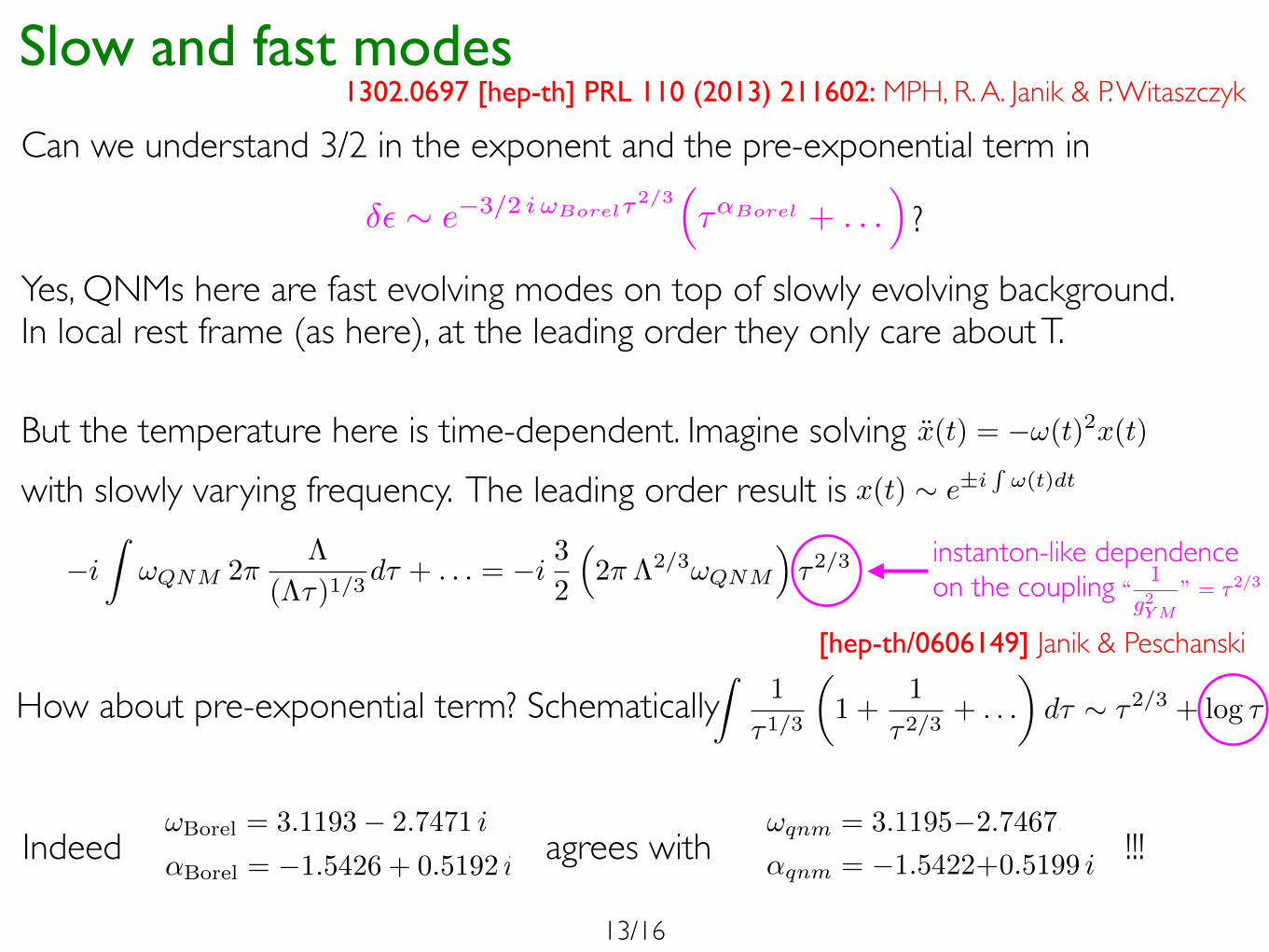
⌘Can we understand 3/2 in the exponent and the pre-exponential term in

?

Yes, QNMs here are fast evolving modes on top of slowly evolving background.In local rest frame (as here), at the leading order they only care about T.

But the temperature here is time-dependent. Imagine solvingwith slowly varying frequency. The leading order result is

�i

Z!QNM 2⇡

⇤

(⇤⌧)1/3d⌧ + . . . = �i

3

2

⇣2⇡⇤2/3!QNM

⌘⌧2/3

[hep-th/0606149] Janik & Peschanski

x(t) = �!(t)2x(t)

x(t) ⇠ e

±iR!(t)dt

instanton-like dependenceon the coupling “

1

g2YM

” = ⌧2/3

How about pre-exponential term? SchematicallyZ

1

⌧1/3

✓1 +

1

⌧2/3+ . . .

◆d⌧ ⇠ ⌧2/3 + log ⌧

Indeed agrees with !!!

2

longitudinal direction. This symmetry can be made man-ifest upon passing to curvilinear proper time ⌧ - rapidityy coordinates related to the lab frame time x

0 and posi-tion along the expansion axis x1 via

x

0 = ⌧ cosh y and x

1 = ⌧ sinh y. (1)

In the case of (3+1)-dimensional conformal field theoryplasma, the most general stress tensor obeying the sym-metries of the problem in coordinates (⌧, y, x1

, x

2) reads

T

µ⌫ = diag(�✏, pL, pT , pT )

µ⌫ , (2)

where the energy density ✏ is a function of proper timeonly and the longitudinal pL and transverse pT pressuresare fully expressed in terms of the energy density [9]

pL = �✏� ⌧ ✏

0 and pT = ✏+1

2⌧ ✏

0. (3)

Note that, in the proper time - rapidity coordinates (1),there is no momentum flow in the stress tensor (2) andso the flow velocity is trivial and takes the form u =@⌧ . Hydrodynamic constituent relations lead, then, togradient expanded energy density of the form

✏ =3

8N

2

c ⇡2

1

⌧

4/3

✓✏

2

+ ✏

3

1

⌧

2/3+ ✏

4

1

⌧

4/3+ . . .

◆, (4)

where the choice of ✏2

sets an overall energy scale, in par-ticular for the quasinormal frequencies (7) and 9). Theprefactor was chosen to match the N = 4 super Yang-Mills theory at large-Nc and strong coupling. In the fol-lowing, we choose the units by setting ✏

2

= ⇡

�4.Large-⌧ expansion of the energy density in powers of

⌧

�2/3, as in (4), is equivalent to the hydrodynamic gra-dient expansion and arises from expressing gradients ofvelocity (rµu⌫ ⇠ ⌧

�1) in units of the e↵ective tempera-ture (T ⇠ ✏

1/4 ⇠ ⌧

�1/3). The value of the coe�cient ✏

3

is related to the shear viscosity ⌘, whereas ✏

4

is a sumof two transport coe�cients: relaxation time ⌧

⇧

and theso-called �

1

[10]. Higher order contributions to the en-ergy density are expected to be linear combinations of sofar unidentified transport coe�cients. Note also that theexpansion (4) is sensitive to both linear and nonlineargradient terms.

As explained in [11, 12] (see also Supplemental ma-terial), higher order contributions to the energy density(4) can be obtained by solving Einstein’s equations witha negative cosmological constant for the metric ansatz ofthe form

ds

2 = 2d⌧dr�Ad⌧

2+⌃2

e

�2Bdy

2+⌃2

e

B(dx2

1

+dx

2

2

), (5)

where the warp factors A, ⌃ and B are functions of rand ⌧ constructed in the gradient expansion as requiredby the fluid-gravity duality. At leading order, the warpfactors are that of a locally boosted black brane and this

solution gets systematically corrected in ⌧

�2/3 expansion,as is the case with the energy density in the dual fieldtheory (4).The background expanded in ⌧

�2/3 around a locallyboosted black brane is slowly evolving and captures onlyhydrodynamic degrees of freedom. One can, in ad-dition, consider the incorporation of nonhydrodynamic(fast evolving) degrees of freedom by linearizing Ein-stein’s equations on top of the hydrodynamic solution,i.e. B = B

hydro

+ �B, and similarly for A and ⌃, andlooking for �B corresponding to (at very large time) theexponentially decaying contribution to the stress tensordepending only on ⌧ . For the static background analo-gous calculation would lead to the spectrum of nonhydro-dynamic quasinormal modes carrying zero momentum,which is known to be the same as the spectrum of zeromomentum quasinormal modes for the massless scalarfield [13].In the leading order of the gradient expansion, the re-

sulting modes, on the gravity side, indeed essentially re-duce to the scalar quasinormal modes but obtain an ad-ditional factor of 3

2

and are damped exponentially in ⌧

2

3

[14]. Upon including viscous correction, the modes ob-tain a further nontrivial powerlike preexponential factor

�✏ ⇠ ⌧

↵qnm exp (�i

3

2!qnm ⌧

2/3). (6)

Explicit gravity calculation for the lowest mode yield

!qnm = 3.1195�2.7467, ↵qnm = �1.5422+0.5199 i. (7)

The frequency !qnm agrees with the frequency of thelowest nonhydrodynamic scalar quasinormal mode andwas calculated before in [14], whereas the prediction of↵qnm is a new result specific to the dissipative modifi-cations of the expanding black hole geometry (see theSupplemental Material for further details). In the fol-lowing, we will be able to reproduce numerically (7) justfrom the large order behavior of the hydrodynamic series.Large order behavior of hydrodynamic energy

density. Numerical implementation of the methods out-lined in [11, 12] allow for e�cient calculation of hydrody-namic series given by (4), up to a very large order, sinceone is e↵ectively solving a set of linear ODE’s (comingfrom Einstein’s equations) at each order. Using spectralmethods we iteratively solved these equations in the largetime expansion reconstructing the energy density up tothe order 240, i.e. up to the term ✏

242

in (4). To the bestof our knowledge this is the first approach allowing us toaccess information about the large order behavior of thehydrodynamic series in any physical system or model.As a way of monitoring the accuracy of our procedures

we compared normalized values of evaluated Einstein’sequations at each order of the ⌧

�2/3 expansion to theratio of coe�cients of gradient-expanded energy densityto gradient expanded warp factors. This ensures thatour results for the energy density are reliable. We also

2

longitudinal direction. This symmetry can be made man-ifest upon passing to curvilinear proper time ⌧ - rapidityy coordinates related to the lab frame time x

0 and posi-tion along the expansion axis x1 via

x

0 = ⌧ cosh y and x

1 = ⌧ sinh y. (1)

In the case of (3+1)-dimensional conformal field theoryplasma, the most general stress tensor obeying the sym-metries of the problem in coordinates (⌧, y, x1

, x

2) reads

T

µ⌫ = diag(�✏, pL, pT , pT )

µ⌫ , (2)

where the energy density ✏ is a function of proper timeonly and the longitudinal pL and transverse pT pressuresare fully expressed in terms of the energy density [9]

pL = �✏� ⌧ ✏

0 and pT = ✏+1

2⌧ ✏

0. (3)

Note that, in the proper time - rapidity coordinates (1),there is no momentum flow in the stress tensor (2) andso the flow velocity is trivial and takes the form u =@⌧ . Hydrodynamic constituent relations lead, then, togradient expanded energy density of the form

✏ =3

8N

2

c ⇡2

1

⌧

4/3

✓✏

2

+ ✏

3

1

⌧

2/3+ ✏

4

1

⌧

4/3+ . . .

◆, (4)

where the choice of ✏2

sets an overall energy scale, in par-ticular for the quasinormal frequencies (7) and 9). Theprefactor was chosen to match the N = 4 super Yang-Mills theory at large-Nc and strong coupling. In the fol-lowing, we choose the units by setting ✏

2

= ⇡

�4.Large-⌧ expansion of the energy density in powers of

⌧

�2/3, as in (4), is equivalent to the hydrodynamic gra-dient expansion and arises from expressing gradients ofvelocity (rµu⌫ ⇠ ⌧

�1) in units of the e↵ective tempera-ture (T ⇠ ✏

1/4 ⇠ ⌧

�1/3). The value of the coe�cient ✏

3

is related to the shear viscosity ⌘, whereas ✏

4

is a sumof two transport coe�cients: relaxation time ⌧

⇧

and theso-called �

1

[10]. Higher order contributions to the en-ergy density are expected to be linear combinations of sofar unidentified transport coe�cients. Note also that theexpansion (4) is sensitive to both linear and nonlineargradient terms.

As explained in [11, 12] (see also Supplemental ma-terial), higher order contributions to the energy density(4) can be obtained by solving Einstein’s equations witha negative cosmological constant for the metric ansatz ofthe form

ds

2 = 2d⌧dr�Ad⌧

2+⌃2

e

�2Bdy

2+⌃2

e

B(dx2

1

+dx

2

2

), (5)

where the warp factors A, ⌃ and B are functions of rand ⌧ constructed in the gradient expansion as requiredby the fluid-gravity duality. At leading order, the warpfactors are that of a locally boosted black brane and this

solution gets systematically corrected in ⌧

�2/3 expansion,as is the case with the energy density in the dual fieldtheory (4).The background expanded in ⌧

�2/3 around a locallyboosted black brane is slowly evolving and captures onlyhydrodynamic degrees of freedom. One can, in ad-dition, consider the incorporation of nonhydrodynamic(fast evolving) degrees of freedom by linearizing Ein-stein’s equations on top of the hydrodynamic solution,i.e. B = B

hydro

+ �B, and similarly for A and ⌃, andlooking for �B corresponding to (at very large time) theexponentially decaying contribution to the stress tensordepending only on ⌧ . For the static background analo-gous calculation would lead to the spectrum of nonhydro-dynamic quasinormal modes carrying zero momentum,which is known to be the same as the spectrum of zeromomentum quasinormal modes for the massless scalarfield [13].In the leading order of the gradient expansion, the re-

sulting modes, on the gravity side, indeed essentially re-duce to the scalar quasinormal modes but obtain an ad-ditional factor of 3

2

and are damped exponentially in ⌧

2

3

[14]. Upon including viscous correction, the modes ob-tain a further nontrivial powerlike preexponential factor

�✏ ⇠ ⌧

↵qnm exp (�i

3

2!qnm ⌧

2/3). (6)

Explicit gravity calculation for the lowest mode yield

!qnm = 3.1195�2.7467, ↵qnm = �1.5422+0.5199 i. (7)

The frequency !qnm agrees with the frequency of thelowest nonhydrodynamic scalar quasinormal mode andwas calculated before in [14], whereas the prediction of↵qnm is a new result specific to the dissipative modifi-cations of the expanding black hole geometry (see theSupplemental Material for further details). In the fol-lowing, we will be able to reproduce numerically (7) justfrom the large order behavior of the hydrodynamic series.Large order behavior of hydrodynamic energy

density. Numerical implementation of the methods out-lined in [11, 12] allow for e�cient calculation of hydrody-namic series given by (4), up to a very large order, sinceone is e↵ectively solving a set of linear ODE’s (comingfrom Einstein’s equations) at each order. Using spectralmethods we iteratively solved these equations in the largetime expansion reconstructing the energy density up tothe order 240, i.e. up to the term ✏

242

in (4). To the bestof our knowledge this is the first approach allowing us toaccess information about the large order behavior of thehydrodynamic series in any physical system or model.As a way of monitoring the accuracy of our procedures

we compared normalized values of evaluated Einstein’sequations at each order of the ⌧

�2/3 expansion to theratio of coe�cients of gradient-expanded energy densityto gradient expanded warp factors. This ensures thatour results for the energy density are reliable. We also

3

FIG. 1. Behavior of the coe�cients of hydrodynamic seriesfor the energy density as a function of the order. At largeenough order the coe�cients start exhibiting factorial growth.The radius of convergence of the Borel transformed series isestimated to be 6.37, in rough agreement with (9): 2/3 ⇥6.37 = 4.25.

verified that we reproduced the known analytic resultsfor the energy density at low ( 3) orders.

As anticipated in the introduction, the coe�cients ofthe gradient expanded energy density (4) that we ob-tained, indicate that the hydrodynamic gradient expan-sion, as seen in the example of boost-invariant flow, haszero radius of convergence. This is clearly visible onFig. 1, which shows the factorial growth with order ofthe coe�cients of the hydrodynamic series for the energydensity (4). Numerical values of coe�cients ✏n, as inEq. (4), can be found in the file “eps.m” included in thesubmission (see also Supplemental Material).Singularities of the Borel transform and quasinor-

mal modes. A standard way of dealing with divergentseries, including perturbative quantum field theories [15],is performing a Borel transform of the original power se-ries (here a series in u ⌘ ⌧

� 2

3 ), ✏n = ✏n/ n!, and subse-quently the Borel resummation

✏resum(⌧) =

Z 1

0

✏(⇣⌧) e�⇣d⇣, (8)

where the integral is taken over the real positive axis.A key issue in performing Borel resummation is the iden-tification of the singularities of the Borel transform andits analytical continuation into some neighborhood of thepositive real axis. The singularities of the Borel trans-form are interesting for their own sake as, typically, theyhave a definite physical interpretation (like instantoncontributions in quantum field theories). We will findthat this will also be the case in our context.

Since the Borel transform has typically only a finiteradius of convergence, we use the standard technique ofPade approximants to provide an analytic continuation.Such an approach was used with success in the context ofresumming perturbative series in quantum field theoriesin [16] and, in principle, can be refined by including the

FIG. 2. Real and imaginary parts of poles ⇣0 of the symmet-ric Pade approximant of the Borel transform of the energydensity (4). From the plot we removed numerically spuriouspoles. The pole closest to the origin governs the convergenceradius of the Borel transformed series and gives rise to thelowest quasinormal frequency. The poles from the encircledregion (magenta) lead to the powerlike preexponential factorin (6).

information about the behavior of the series at large val-ues of the parameter (typically strong coupling behaviorfor perturbative expansion in quantum field theories).In our case, this regime corresponds to small times

(high order dissipative terms). Although it was estab-lished that, when expanded around ⌧ = 0, the energydensity contains only even powers of proper time [17],this information turns out to be hard to implement in anunambiguous way and, in the following, we adopted thesimplest analytic continuation.Figure 2 shows the position of poles of the symmetric

Pade approximant of the Borel transformed energy den-sity. Let us note that some care must be taken as thePade approximant exhibits apparent poles on the nega-tive real axis which, however, cancel almost perfectly (upto 10�100 accuracy) with zeroes of the numerator. As ourknowledge about the series is limited to a finite numberof terms (first 241), we should only trust the structurein the close vicinity of the origin. Note, however, thatthe lack of poles on the positive real axis seems to in-dicate Borel summability, pointing towards the possibleexistence of Borel-resummed all-order hydrodynamics.The poles approximate some complicated structure of

branch cuts. The pole nearest the origin, from which amajor branch cut starts, sets the radius of convergenceof the Borel transform of hydrodynamic series. Its nu-merical value (multiplied by the factor 3/2i) reads

!

Borel

= 3.1193� 2.7471 i (|!Borel

| = 4.1565) (9)

and is consistent with the coe�cient obtained from fittingfactorial-like behavior of the original series.Deforming the contour from the real positive axis to

the one encircling some of the zeros of the denomina-tor of the Pade approximated Borel transform, through

4

residues, leads to an ambiguity in resummation. It istempting to speculate that such an ambiguity can be un-derstood as the appearance of new, nonhydrodynamic,degrees of freedom in the system. Indeed, perform-ing contour integration around the cut originating from(3/2i)⇥ !

Borel

leads to the following contribution to theenergy density at large proper time

�✏ ⇠ ⌧

↵Borel exp (�i

3

2!

Borel

⌧

2/3), (10)

where

↵

Borel

= �1.5426 + 0.5192 i. (11)

The contribution (10) together with (9) and (11)matches, up to numerical accuracy, the gravitational pre-diction for the behavior of the lowest metric quasinormalmode given by (6) and (7), but is derived entirely withinthe hydrodynamic gradient expansion.Summary and conclusions. We used the fluid-gravityduality to numerically obtain the form of hydrodynamicstress tensor of the Bjorken flow up to 240th order in gra-dients. This corresponds to the inclusion of dissipativeterms of a very high order. We discovered that the cor-rections grow factorially with the order. This providesstrong indication that hydrodynamic expansion is an ex-ample of asymptotic series; i.e., it has a zero radius ofconvergence.

Upon a simple analytic continuation of Borel trans-formed series we found that it is the frequency of thelowest nonhydrodynamic quasinormal mode which setsthe radius of convergence of the Borel transform. Subse-quently, from the hydrodynamic expression alone we ex-tracted the modification of this contribution due to theshear viscosity and matched with the gravity calculation.It is fascinating to observe that nonhydrodynamic col-lective excitations, which are not describable within theframework of hydrodynamics, nevertheless leave their im-print in the behavior of high order transport coe�cients.This is reminiscent of the relation of instanton contri-butions with the divergence of the perturbative series inquantum field theory.

Note that our observation about the asymptotic char-acter of the hydrodynamic series is made upon evaluatingthe stress tensor of a particular type of hydrodynamicflow. The high degree of symmetry of that flow – boost-invariance – means that at each order in the large propertime expansion, we are indeed studying new dissipativeterms in the hydrodynamic stress tensor with new trans-port coe�cients. The dependence on initial conditionsfor this hydrodynamic flow reduces just to a trivial over-all rescaling.

We speculate that the most likely source of the facto-rial growth of the coe�cients of the hydrodynamic seriesfor the energy density is the fast growth of the number ofgradient terms contributing to the hydrodynamic stress

tensor at each order, in analogy with the factorial growthof the number of Feynman graphs at large order of per-turbative calculations.

Regarding future directions, a thought-provoking phe-nomenological spin o↵ of our Letter is the possibility ofresumming hydrodynamic description and extending thehydrodynamic stress tensor past the regime in which sub-sequent low order terms give comparable contributions.This might lead to refined criterium for the applicabilityof hydrodynamics used in [2, 3] and goes very much inthe spirit of [4, 5].

Acknowledgments. MPH acknowledges support fromthe Netherlands Organization for Scientific Research un-der the Veni scheme and would like to thank Norditafor hospitality. This work was supported by NCNgrant 2012/06/A/ST2/00396 (RJ) and IoP JU grantK/DSC/000705 (PW). PW would like to thank theLorentz Center and Nordita for hospitality. We used M.Headrick’s diffgeo.m package for symbolic GR. Finallywe would like to thank M. Baggio, J. de Boer, K. Land-steiner, C. Nunez and D. Teaney for interesting discus-sions and suggestions.

⇤ m.p.heller@uva.nl; On leave from: National Centre forNuclear Research, Hoza 69, 00-681 Warsaw, Poland

† romuald@th.if.uj.edu.pl‡ bofh@th.if.uj.edu.pl

[1] U. W. Heinz and R. Snellings, arXiv:1301.2826 [nucl-th].[2] M. P. Heller, R. A. Janik and P. Witaszczyk, Phys. Rev.

Lett. 108, 201602 (2012) [arXiv:1103.3452 [hep-th]].[3] M. P. Heller, R. A. Janik and P. Witaszczyk, Phys. Rev.

D 85, 126002 (2012) [arXiv:1203.0755 [hep-th]].[4] M. Lublinsky and E. Shuryak, Phys. Rev. C 76, 021901

(2007) [arXiv:0704.1647 [hep-ph]].[5] M. Lublinsky and E. Shuryak, Phys. Rev. D 80, 065026

(2009) [arXiv:0905.4069 [hep-ph]].[6] J. M. Maldacena, Adv. Theor. Math. Phys. 2, 231

(1998) [Int. J. Theor. Phys. 38, 1113 (1999)] [arXiv:hep-th/9711200].

[7] S. Bhattacharyya, V. E. Hubeny, S. Minwalla andM. Rangamani, JHEP 0802, 045 (2008) [arXiv:0712.2456[hep-th]].

[8] J. D. Bjorken, Phys. Rev. D 27, 140 (1983).[9] R. A. Janik and R. B. Peschanski, Phys. Rev. D 73,

045013 (2006) [arXiv:hep-th/0512162].[10] R. Baier, P. Romatschke, D. T. Son, A. O. Starinets

and M. A. Stephanov, JHEP 0804, 100 (2008)[arXiv:0712.2451 [hep-th]].

[11] M. P. Heller, P. Surowka, R. Loganayagam, M. Spalinskiand S. E. Vazquez, Phys. Rev. Lett. 102, 041601 (2009)[arXiv:0805.3774 [hep-th]].

[12] S. Kinoshita, S. Mukohyama, S. Nakamura andK. -y. Oda, Prog. Theor. Phys. 121, 121 (2009)[arXiv:0807.3797 [hep-th]].

[13] P. K. Kovtun and A. O. Starinets, Phys. Rev. D 72,086009 (2005) [hep-th/0506184].

[14] R. A. Janik and R. B. Peschanski, Phys. Rev. D 74,

Interpretationand possible relevance

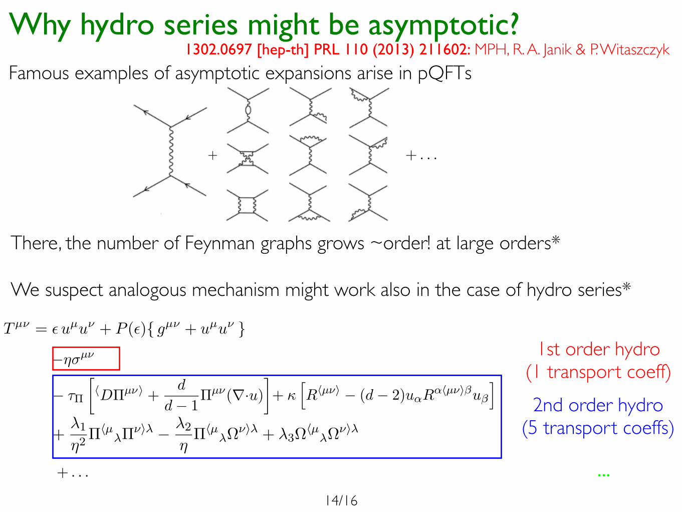
Famous examples of asymptotic expansions arise in pQFTsMPH, R. A. Janik & P. Witaszczyk

There, the number of Feynman graphs grows ~order! at large orders*

We suspect analogous mechanism might work also in the case of hydro series*

Tµ⌫ = ✏uµu⌫ + P (✏){ gµ⌫ + uµu⌫ }� ⌘(✏)�µ⌫ � ⇣(✏){ gµ⌫ + uµu⌫ }(r · u) + . . .

With the restriction of transversality and tracelessness, there are eight possible contribu-

tions to the stress-energy tensor:

!!µ ln T !!" ln T, !!µ!!" ln T, !µ!(!·u), !!µ"!!""

!!µ"!!"", !!µ

"!!"", u#R#!µ!"$u$, R!µ!" .(3.6)

By direct computations we find that there are only five combinations that transform

homogeneously under Weyl tranformations. They are

Oµ!1 = R!µ!" " (d " 2)

!

!!µ!!" ln T "!!µ ln T !!" ln T"

, (3.7)

Oµ!2 = R!µ!" " (d " 2)u#R#!µ!"$u$ , (3.8)

Oµ!3 = !!µ

"!!"" , Oµ!4 = !!µ

"!!"" , Oµ!5 = !!µ

"!!"" . (3.9)

In the linearized hydrodynamics in flat space only the term Oµ!1 contributes. For conve-

nience and to facilitate the comparision with the Israel-Stewart theory we shall use instead

of (3.7) the term!D!µ! " +

1

d " 1!µ!(!·u) (3.10)

which, with (3.5), reduces to the linear combination: Oµ!1 " Oµ!

2 " (1/2)Oµ!3 " 2Oµ!

5 . It is

straightforward to check directly that (3.10) transforms homogeneously under Weyl transfor-

mations.

Thus, our final expression for the dissipative part of the stress-energy tensor, up to second

order in derivatives, is

"µ! = ""!µ!

+ "#!

#

!D!µ! " +1

d " 1!µ!(!·u)

$

+ $%

R!µ!" " (d " 2)u#R#!µ!"$u$

&

+ %1!!µ

"!!"" + %2!!µ

"!!"" + %3!!µ

"!!"" .

(3.11)

The five new constants are #!, $, %1,2,3. Note that using lowest order relations "µ! = ""!µ! ,

Eqs.(3.5) and D" = ""!·u, Eq. (3.11) may be rewritten in the form

"µ! = ""!µ! " #!

#

!D"µ! " +d

d " 1"µ!(!·u)

$

+ $%

R!µ!" " (d " 2)u#R#!µ!"$u$

&

+%1

"2"!µ

""!"" " %2

""!µ

"!!"" + %3!!µ

"!!"" .

(3.12)

This equation is, in form, similar to an equation of the Israel-Stewart theory (see Section 6).

In the linear regime it actually coincides with the Israel-Stewart theory (6.1). We emphasize,

however, that one cannot claim that Eq. (3.12) captures all orders in the momentum expansion

(see Section 6).

– 8 –

With the restriction of transversality and tracelessness, there are eight possible contribu-

tions to the stress-energy tensor:

!!µ ln T !!" ln T, !!µ!!" ln T, !µ!(!·u), !!µ"!!""

!!µ"!!"", !!µ

"!!"", u#R#!µ!"$u$, R!µ!" .(3.6)

By direct computations we find that there are only five combinations that transform

homogeneously under Weyl tranformations. They are

Oµ!1 = R!µ!" " (d " 2)

!

!!µ!!" ln T "!!µ ln T !!" ln T"

, (3.7)

Oµ!2 = R!µ!" " (d " 2)u#R#!µ!"$u$ , (3.8)

Oµ!3 = !!µ

"!!"" , Oµ!4 = !!µ

"!!"" , Oµ!5 = !!µ

"!!"" . (3.9)

In the linearized hydrodynamics in flat space only the term Oµ!1 contributes. For conve-

nience and to facilitate the comparision with the Israel-Stewart theory we shall use instead

of (3.7) the term!D!µ! " +

1

d " 1!µ!(!·u) (3.10)

which, with (3.5), reduces to the linear combination: Oµ!1 " Oµ!

2 " (1/2)Oµ!3 " 2Oµ!

5 . It is

straightforward to check directly that (3.10) transforms homogeneously under Weyl transfor-

mations.

Thus, our final expression for the dissipative part of the stress-energy tensor, up to second

order in derivatives, is

"µ! = ""!µ!

+ "#!

#

!D!µ! " +1

d " 1!µ!(!·u)

$

+ $%

R!µ!" " (d " 2)u#R#!µ!"$u$

&

+ %1!!µ

"!!"" + %2!!µ

"!!"" + %3!!µ

"!!"" .

(3.11)

The five new constants are #!, $, %1,2,3. Note that using lowest order relations "µ! = ""!µ! ,

Eqs.(3.5) and D" = ""!·u, Eq. (3.11) may be rewritten in the form

"µ! = ""!µ! " #!

#

!D"µ! " +d

d " 1"µ!(!·u)

$

+ $%

R!µ!" " (d " 2)u#R#!µ!"$u$

&

+%1

"2"!µ

""!"" " %2

""!µ

"!!"" + %3!!µ

"!!"" .

(3.12)

This equation is, in form, similar to an equation of the Israel-Stewart theory (see Section 6).

In the linear regime it actually coincides with the Israel-Stewart theory (6.1). We emphasize,

however, that one cannot claim that Eq. (3.12) captures all orders in the momentum expansion

(see Section 6).

– 8 –

With the restriction of transversality and tracelessness, there are eight possible contribu-

tions to the stress-energy tensor:

!!µ ln T !!" ln T, !!µ!!" ln T, !µ!(!·u), !!µ"!!""

!!µ"!!"", !!µ

"!!"", u#R#!µ!"$u$, R!µ!" .(3.6)

By direct computations we find that there are only five combinations that transform

homogeneously under Weyl tranformations. They are

Oµ!1 = R!µ!" " (d " 2)

!

!!µ!!" ln T "!!µ ln T !!" ln T"

, (3.7)

Oµ!2 = R!µ!" " (d " 2)u#R#!µ!"$u$ , (3.8)

Oµ!3 = !!µ

"!!"" , Oµ!4 = !!µ

"!!"" , Oµ!5 = !!µ

"!!"" . (3.9)

In the linearized hydrodynamics in flat space only the term Oµ!1 contributes. For conve-

nience and to facilitate the comparision with the Israel-Stewart theory we shall use instead

of (3.7) the term!D!µ! " +

1

d " 1!µ!(!·u) (3.10)

which, with (3.5), reduces to the linear combination: Oµ!1 " Oµ!

2 " (1/2)Oµ!3 " 2Oµ!

5 . It is

straightforward to check directly that (3.10) transforms homogeneously under Weyl transfor-

mations.

Thus, our final expression for the dissipative part of the stress-energy tensor, up to second

order in derivatives, is

"µ! = ""!µ!

+ "#!

#

!D!µ! " +1

d " 1!µ!(!·u)

$

+ $%

R!µ!" " (d " 2)u#R#!µ!"$u$

&

+ %1!!µ

"!!"" + %2!!µ

"!!"" + %3!!µ

"!!"" .

(3.11)

The five new constants are #!, $, %1,2,3. Note that using lowest order relations "µ! = ""!µ! ,

Eqs.(3.5) and D" = ""!·u, Eq. (3.11) may be rewritten in the form

"µ! = ""!µ! " #!

#

!D"µ! " +d

d " 1"µ!(!·u)

$

+ $%

R!µ!" " (d " 2)u#R#!µ!"$u$

&

+%1

"2"!µ

""!"" " %2

""!µ

"!!"" + %3!!µ

"!!"" .

(3.12)

This equation is, in form, similar to an equation of the Israel-Stewart theory (see Section 6).

In the linear regime it actually coincides with the Israel-Stewart theory (6.1). We emphasize,

however, that one cannot claim that Eq. (3.12) captures all orders in the momentum expansion

(see Section 6).

– 8 –

With the restriction of transversality and tracelessness, there are eight possible contribu-

tions to the stress-energy tensor:

!!µ ln T !!" ln T, !!µ!!" ln T, !µ!(!·u), !!µ"!!""

!!µ"!!"", !!µ

"!!"", u#R#!µ!"$u$, R!µ!" .(3.6)

By direct computations we find that there are only five combinations that transform

homogeneously under Weyl tranformations. They are

Oµ!1 = R!µ!" " (d " 2)

!

!!µ!!" ln T "!!µ ln T !!" ln T"

, (3.7)

Oµ!2 = R!µ!" " (d " 2)u#R#!µ!"$u$ , (3.8)

Oµ!3 = !!µ

"!!"" , Oµ!4 = !!µ

"!!"" , Oµ!5 = !!µ

"!!"" . (3.9)

In the linearized hydrodynamics in flat space only the term Oµ!1 contributes. For conve-

nience and to facilitate the comparision with the Israel-Stewart theory we shall use instead

of (3.7) the term!D!µ! " +

1

d " 1!µ!(!·u) (3.10)

which, with (3.5), reduces to the linear combination: Oµ!1 " Oµ!

2 " (1/2)Oµ!3 " 2Oµ!

5 . It is

straightforward to check directly that (3.10) transforms homogeneously under Weyl transfor-

mations.

Thus, our final expression for the dissipative part of the stress-energy tensor, up to second

order in derivatives, is

"µ! = ""!µ!

+ "#!

#

!D!µ! " +1

d " 1!µ!(!·u)

$

+ $%

R!µ!" " (d " 2)u#R#!µ!"$u$

&

+ %1!!µ

"!!"" + %2!!µ

"!!"" + %3!!µ

"!!"" .

(3.11)

The five new constants are #!, $, %1,2,3. Note that using lowest order relations "µ! = ""!µ! ,

Eqs.(3.5) and D" = ""!·u, Eq. (3.11) may be rewritten in the form

"µ! = ""!µ! " #!

#

!D"µ! " +d

d " 1"µ!(!·u)

$

+ $%

R!µ!" " (d " 2)u#R#!µ!"$u$

&

+%1

"2"!µ

""!"" " %2

""!µ

"!!"" + %3!!µ

"!!"" .

(3.12)

This equation is, in form, similar to an equation of the Israel-Stewart theory (see Section 6).

In the linear regime it actually coincides with the Israel-Stewart theory (6.1). We emphasize,

however, that one cannot claim that Eq. (3.12) captures all orders in the momentum expansion

(see Section 6).

– 8 –

+ . . .

1st order hydro (1 transport coeff)2nd order hydro

(5 transport coeffs)

...

Why hydro series might be asymptotic?

+ . . .+

1302.0697 [hep-th] PRL 110 (2013) 211602:

14/16

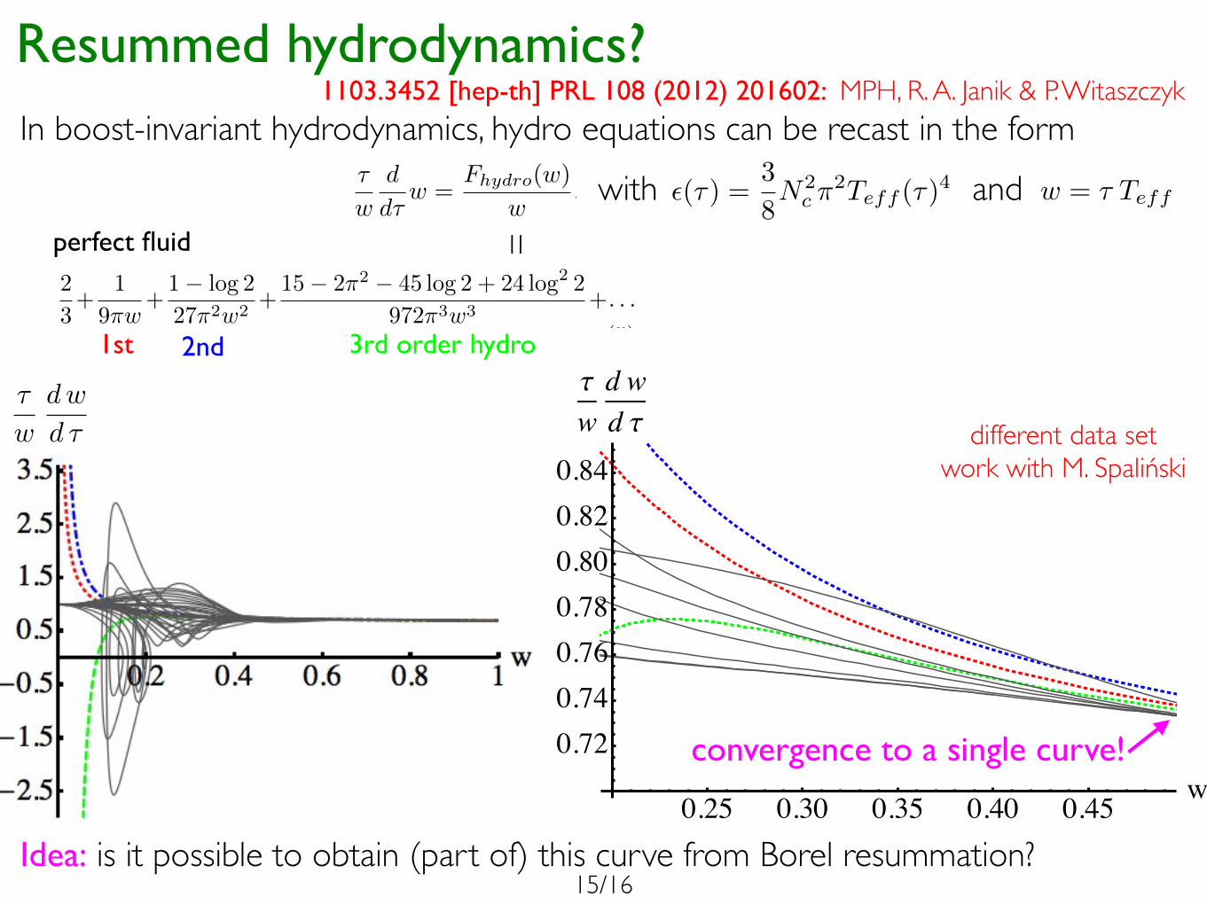
Resummed hydrodynamics?In boost-invariant hydrodynamics, hydro equations can be recast in the form

2

solution at the AdS boundary. The details will apear in asubsequent paper [11], while in the present letter we willconcentrate on the physical questions mentioned above.

Boost-invariant plasma and hydrodynamics. Thetraceless and conserved energy-momentum tensor of aboost-invariant conformal plasma system with no trans-verse coordinate dependence is uniquely determined interms of a single function ⇧T⇤⇤ ⌃ – the energy density atmid-rapidity ⇤(⇥). The longitudinal and transverse pres-sure are consequently given by

pL = �⇤� ⇥d

d⇥⇤ and pT = ⇤+

1

2⇥d

d⇥⇤ . (1)

It is quite convenient to eliminate explicit dependenceon the number of colors Nc and degrees of freedom byintroducing an e�ective temperature Teff through

⇧T⇤⇤ ⌃ ⇤ ⇤(⇥) ⇤ N2c · 3

8�2 · T 4

eff . (2)

Let us emphasize that Teff does not imply in any waythermalization. It just measures the temperature of athermal system with an identical energy density as ⇤(⇥).

All order viscous hydrodynamics amounts to present-ing the energy-momentum tensor as a series of terms ex-pressed in terms of flow velocities uµ and their deriva-tives with coe⌅cients being proportional to appropriatepowers of Teff , the proportionality constants being thetransport coe⌅cients. For the case of N = 4 plasma,the above mentioned form of Tµ⇥ is not an assumptionbut a result of a derivation from AdS/CFT [7]. Hydro-dynamic equations are just the conservation equations µTµ⇥ = 0, which are by construction first-order di�er-ential equations for Teff .

In the case of boost-invariant conformal plasma thisleads to a universal form of first order dynamical equa-tions for the scale invariant quantity

w = Teff · ⇥ (3)

namely

⇥

w

d

d⇥w =

Fhydro(w)

w, (4)

where Fhydro(w) is completely determined in terms of thetransport coe⌅cients of the theory1. For N = 4 plasmaat strong coupling Fhydro(w)/w is known explicitly up toterms corresponding to 3rd order hydrodynamics [13]

2

3+

1

9�w+1� log 2

27�2w2+15� 2�2 � 45 log 2 + 24 log2 2

972�3w3+. . .

(5)

1This is quite reminiscent of [12] where all-order hydrodynamics

was postulated in terms of linearized AdS dynamics.

0 0.2 0.4 0.6 0.8w

0.4

0.8

1.2

F �w⇥w

FIG. 1. a) F (w)/w versus w for various initial data. b)Pressure anisotropy 1 � 3pL

� and for a selected profile. Red,

blue and green curves correspond to 1st, 2nd and 3rd orderhydrodynamics respectively.

The importance of formula (4) lies in the fact that if theplasma dynamics would be governed entirely by (evenresummed) hydrodynamics including dissipative termsof arbitrarily high degree, then on a plot of ⇤

wdd⇤w ⇤

F (w)/w as a function of w trajectories for all initial con-ditions would lie on a single curve given by Fhydro(w)/w.If, on the other hand, genuine nonequilibrium processeswould intervene we would observe a wide range of curveswhich would merge for su⌅ciently large w when thermal-ization and transition to hydrodynamics would occur.In Figure 1a we present this plot for 20 trajectories

corresponding to 20 di�erent initial states. It is clearfrom the plot that nonhydrodynamic modes are veryimportant in the initial stage of plasma evolution, yetfor all the sets of initial data, for w > 0.65 the curvesmerge into a single curve characteristic of hydrodynam-ics. In Figure 1b we show a plot of pressure anisotropy1� 3pL

⌅ ⇤ 12F (w)w � 8 for a selected profile and compare

this with the corresponding curves for 1st, 2nd and 3rd

order hydrodynamics. We observe on this example, onthe one hand, a perfect agreement with hydrodynamicsfor w > 0.63 and, on the other hand, a quite sizeablepressure anisotropy in that regime which is neverthelesscompletely explained by dissipative hydrodynamics.In order to study the transition to hydrodynamics in

more detail, we will adopt a numerical criterion for ther-malization which is the deviation of ⇥ d

d⇤w from the 3rd

order hydro expression (5)�����

⇥ dd⇤w

F 3rd orderhydro (w)

� 1

����� < 0.005. (6)

Despite the bewildering variety of the nonequilibriumevolution, we will show below that there exist, however,some surprising regularities in the dynamics.

Initial and final entropy. Apart from the energy-momentum tensor components, a very important physi-cal property of the evolving plasma system is its entropydensity S (per transverse area and unit (spacetime) ra-pidity). In the general time-dependent case, the precise

=

2

solution at the AdS boundary. The details will apear in asubsequent paper [11], while in the present letter we willconcentrate on the physical questions mentioned above.

Boost-invariant plasma and hydrodynamics. Thetraceless and conserved energy-momentum tensor of aboost-invariant conformal plasma system with no trans-verse coordinate dependence is uniquely determined interms of a single function ⇧T⇤⇤ ⌃ – the energy density atmid-rapidity ⇤(⇥). The longitudinal and transverse pres-sure are consequently given by

pL = �⇤� ⇥d

d⇥⇤ and pT = ⇤+

1

2⇥d

d⇥⇤ . (1)

It is quite convenient to eliminate explicit dependenceon the number of colors Nc and degrees of freedom byintroducing an e�ective temperature Teff through

⇧T⇤⇤ ⌃ ⇤ ⇤(⇥) ⇤ N2c · 3

8�2 · T 4

eff . (2)

Let us emphasize that Teff does not imply in any waythermalization. It just measures the temperature of athermal system with an identical energy density as ⇤(⇥).

All order viscous hydrodynamics amounts to present-ing the energy-momentum tensor as a series of terms ex-pressed in terms of flow velocities uµ and their deriva-tives with coe⌅cients being proportional to appropriatepowers of Teff , the proportionality constants being thetransport coe⌅cients. For the case of N = 4 plasma,the above mentioned form of Tµ⇥ is not an assumptionbut a result of a derivation from AdS/CFT [7]. Hydro-dynamic equations are just the conservation equations µTµ⇥ = 0, which are by construction first-order di�er-ential equations for Teff .

In the case of boost-invariant conformal plasma thisleads to a universal form of first order dynamical equa-tions for the scale invariant quantity

w = Teff · ⇥ (3)

namely

⇥

w

d

d⇥w =

Fhydro(w)

w, (4)

where Fhydro(w) is completely determined in terms of thetransport coe⌅cients of the theory1. For N = 4 plasmaat strong coupling Fhydro(w)/w is known explicitly up toterms corresponding to 3rd order hydrodynamics [13]

2

3+

1

9�w+1� log 2

27�2w2+15� 2�2 � 45 log 2 + 24 log2 2

972�3w3+. . .

(5)

1This is quite reminiscent of [12] where all-order hydrodynamics

was postulated in terms of linearized AdS dynamics.

0 0.2 0.4 0.6 0.8w

0.4

0.8

1.2

F �w⇥w

FIG. 1. a) F (w)/w versus w for various initial data. b)Pressure anisotropy 1 � 3pL

� and for a selected profile. Red,

blue and green curves correspond to 1st, 2nd and 3rd orderhydrodynamics respectively.

The importance of formula (4) lies in the fact that if theplasma dynamics would be governed entirely by (evenresummed) hydrodynamics including dissipative termsof arbitrarily high degree, then on a plot of ⇤

wdd⇤w ⇤

F (w)/w as a function of w trajectories for all initial con-ditions would lie on a single curve given by Fhydro(w)/w.If, on the other hand, genuine nonequilibrium processeswould intervene we would observe a wide range of curveswhich would merge for su⌅ciently large w when thermal-ization and transition to hydrodynamics would occur.In Figure 1a we present this plot for 20 trajectories

corresponding to 20 di�erent initial states. It is clearfrom the plot that nonhydrodynamic modes are veryimportant in the initial stage of plasma evolution, yetfor all the sets of initial data, for w > 0.65 the curvesmerge into a single curve characteristic of hydrodynam-ics. In Figure 1b we show a plot of pressure anisotropy1� 3pL

⌅ ⇤ 12F (w)w � 8 for a selected profile and compare

this with the corresponding curves for 1st, 2nd and 3rd

order hydrodynamics. We observe on this example, onthe one hand, a perfect agreement with hydrodynamicsfor w > 0.63 and, on the other hand, a quite sizeablepressure anisotropy in that regime which is neverthelesscompletely explained by dissipative hydrodynamics.In order to study the transition to hydrodynamics in

more detail, we will adopt a numerical criterion for ther-malization which is the deviation of ⇥ d

d⇤w from the 3rd

order hydro expression (5)�����

⇥ dd⇤w

F 3rd orderhydro (w)

� 1

����� < 0.005. (6)

Despite the bewildering variety of the nonequilibriumevolution, we will show below that there exist, however,some surprising regularities in the dynamics.

Initial and final entropy. Apart from the energy-momentum tensor components, a very important physi-cal property of the evolving plasma system is its entropydensity S (per transverse area and unit (spacetime) ra-pidity). In the general time-dependent case, the precise

perfect fluid

1st 2nd 3rd order hydro

�(⇤) =3

8N2

c ⇥2Teff (⇤)

4 w = � Teffwith and

0.25 0.30 0.35 0.40 0.45 w0.720.740.760.780.800.820.84

twd wd t different data set

work with M. Spaliński

⌧

w

dw

d ⌧

convergence to a single curve!

MPH, R. A. Janik & P. Witaszczyk1103.3452 [hep-th] PRL 108 (2012) 201602:

Idea: is it possible to obtain (part of) this curve from Borel resummation?15/16

Summary

Summary

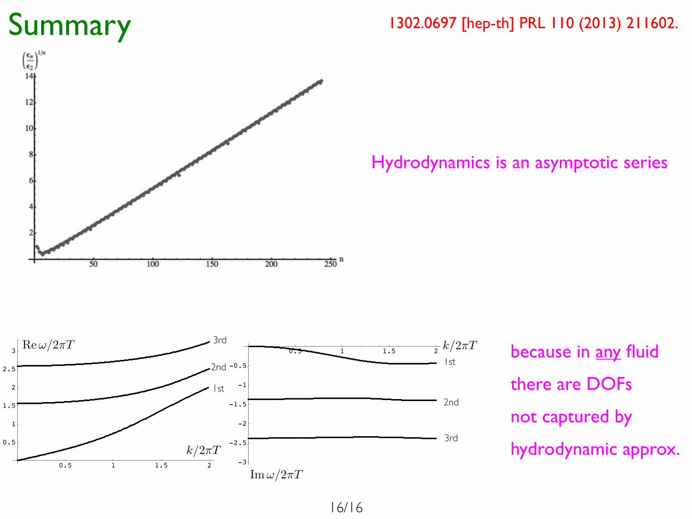
Hydrodynamics is an asymptotic series

1302.0697 [hep-th] PRL 110 (2013) 211602.

16/16

0.5 1 1.5 2

0.5

1

1.5

2

2.5

3 Re 0.5 1 1.5 2

-3

-2.5

-2

-1.5

-1

-0.5

Im

Figure 6: Real and imaginary parts of three lowest quasinormal frequencies as function of spatialmomentum. The curves for which !0 as !0 correspond to hydrodynamic sound mode in the dualfinite temperature N=4 SYM theory.

behavior of the lowest (hydrodynamic) frequency which is absent for E! and Z3. For Ez and

Z1, hydrodynamic frequencies are purely imaginary (given by Eqs. (4.16) and (4.32) for small

! and q), and presumably move o! to infinity as q becomes large. For Z2, the hydrodynamic

frequency has both real and imaginary parts (given by Eq. (4.44) for small ! and q), and

eventually (for large q) becomes indistinguishable in the tower of other eigenfrequencies. As an

example, dispersion relations for the three lowest quasinormal frequencies in the sound channel

(including the one of the sound wave) are shown in Fig. 6. The tables below give numerical

values of quasinormal frequencies for = 1. Only non-hydrodynamic frequencies are shown

in the tables. The position of hydrodynamic frequencies at = 1 is = "3.250637i for the

R-charge di!usive mode, = "0.598066i for the shear mode, and = ±0.741420"0.286280i

for the sound mode. The numerical values of the lowest five (non-hydrodynamic) quasinormal

frequencies for electromagnetic perturbations are:

Transverse channel Di!usive channel

n Re Im Re Im

1 ±1.547187 "0.849723 ±1.147831 "0.559204

2 ±2.398903 "1.874343 ±1.910006 "1.758065

3 ±3.323229 "2.894901 ±2.903293 "2.891681

4 ±4.276431 "3.909583 ±3.928555 "3.943386

5 ±5.244062 "4.920336 ±4.946818 "4.965186

and for gravitational perturbations are:

Scalar channel Shear channel Sound channel

n Re Im Re Im Re Im

1 ±1.954331 "1.267327 ±1.759116 "1.291594 ±1.733511 "1.343008

2 ±2.880263 "2.297957 ±2.733081 "2.330405 ±2.705540 "2.357062

3 ±3.836632 "3.314907 ±3.715933 "3.345343 ±3.689392 "3.363863

4 ±4.807392 "4.325871 ±4.703643 "4.353487 ±4.678736 "4.367981

5 ±5.786182 "5.333622 ±5.694472 "5.358205 ±5.671091 "5.370784

– 26 –

Im!/2⇡T

Re!/2⇡T

k/2⇡T

k/2⇡T

1st

2nd

3rd

1st

2nd

3rd

because in any fluid

there are DOFs

not captured by

hydrodynamic approx.