home page functional principal components analysis · the goal of principal... defining...
TRANSCRIPT

The goal of principal . . .
Defining functional . . .
Home Page
Title Page
JJ II
J I
Page 1 of 28
Go Back
Full Screen
Close
Quit
Functional principalcomponents analysis

The goal of principal . . .
Defining functional . . .
Home Page
Title Page
JJ II
J I
Page 2 of 28
Go Back
Full Screen
Close
Quit
1. The goal of principal componentsanalysis
• PCA is usually used when we want to find the dominantmodes of variation in the data, usually after subtractingthe mean from each observation.
• We want to know how many of these modes of variationare required to achieve a satisfactory approximation tothe original data.
• It may be assumed that keeping only dominant modeswill improve the signal–to–noise ratio of what we keep.
• We usually want to know what these modes representin terms that we can explain to non–statisticians. Rota-tion of the principal components can help at this point.

The goal of principal . . .
Defining functional . . .
Home Page
Title Page
JJ II
J I
Page 3 of 28
Go Back
Full Screen
Close
Quit
2. Defining functional PCA
• Let’s see what changes when we go from the multivari-ate version to the functional version.
• The short answer: Summations change into integra-tions
The goal of principal . . .
Defining functional . . .
Home Page
Title Page
JJ II
J I
Page 4 of 28
Go Back
Full Screen
Close
Quit
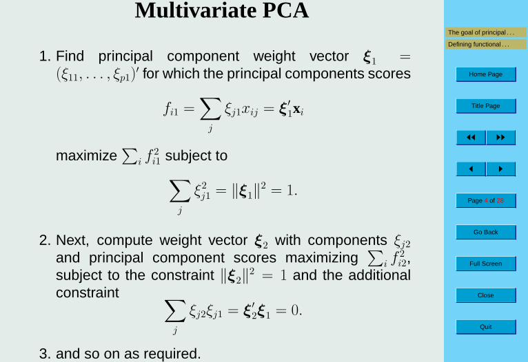
Multivariate PCA
1. Find principal component weight vector ξ1 =(ξ11, . . . , ξp1)
′ for which the principal components scores
fi1 =∑
j
ξj1xij = ξ′1xi
maximize∑
i f2i1 subject to∑
j
ξ2j1 = ‖ξ1‖2 = 1.
2. Next, compute weight vector ξ2 with components ξj2and principal component scores maximizing
∑i f
2i2,
subject to the constraint ‖ξ2‖2 = 1 and the additionalconstraint ∑
j
ξj2ξj1 = ξ′2ξ1 = 0.
3. and so on as required.

The goal of principal . . .
Defining functional . . .
Home Page
Title Page
JJ II
J I
Page 5 of 28
Go Back
Full Screen
Close
Quit
Functional PCA
1. Find principal component weight function ξ1(s) for whichthe principal components scores
fi1 =
∫ξ1(s)xi(s) ds
maximize∑
i f2i1 subject to∫
ξ21(s) ds = ‖ξ1‖2 = 1.
2. Next, compute weight function ξ2(s) and principal com-ponent scores maximizing
∑i f
2i2, subject to the con-
straint ‖ξ2‖2 = 1 and the additional constraint∫ξ2(s)ξ1(s) ds = 0.
3. and so on as required.

The goal of principal . . .
Defining functional . . .
Home Page
Title Page
JJ II
J I
Page 6 of 28
Go Back
Full Screen
Close
Quit
3. A PCA of monthly temperaturecurves
• We have 30-year average temperatures for each monthand for each of 35 Canadian weather stations.

The goal of principal . . .
Defining functional . . .
Home Page
Title Page
JJ II
J I
Page 7 of 28
Go Back
Full Screen
Close
Quit
The centered monthly temperaturecurves

The goal of principal . . .
Defining functional . . .
Home Page
Title Page
JJ II
J I
Page 8 of 28
Go Back
Full Screen
Close
Quit
What do we see?
• An impression that some curves are high (warm) andthat some curves are low (cold).
• Also that some curves have larger variation betweensummer and winter than others.
• How much of the variation do these two types of varia-tion account for?

The goal of principal . . .
Defining functional . . .
Home Page
Title Page
JJ II
J I
Page 9 of 28
Go Back
Full Screen
Close
Quit
The correlation surface

The goal of principal . . .
Defining functional . . .
Home Page
Title Page
JJ II
J I
Page 10 of 28
Go Back
Full Screen
Close
Quit
What do we see?
• The diagonal ridge corresponding to unit correlation be-tween temperatures at identical times.
• The ridge perpendicular to this corresponding to cor-relations between temperatures symmetrically placedaround mid–summer.
• Correlations fall off much more rapidly for times sym-metric about March and September 21.

The goal of principal . . .
Defining functional . . .
Home Page
Title Page
JJ II
J I
Page 11 of 28
Go Back
Full Screen
Close
Quit
The first four principal components

The goal of principal . . .
Defining functional . . .
Home Page
Title Page
JJ II
J I
Page 12 of 28
Go Back
Full Screen
Close
Quit
What do we see?
• The two components that we saw in the centeredcurves account for about 98% of the variation.
• The first four components account for 99.8% of the vari-ation.
• The first four components tend to look like linear,quadratic, cubic and quartic polynomials, respectively.Why is that?
• It can help to plot the components by adding and sub-tracting a multiple of them from the mean function.

The goal of principal . . .
Defining functional . . .
Home Page
Title Page
JJ II
J I
Page 13 of 28
Go Back
Full Screen
Close
Quit
The first four principal components +/-mean

The goal of principal . . .
Defining functional . . .
Home Page
Title Page
JJ II
J I
Page 14 of 28
Go Back
Full Screen
Close
Quit
The first two principal componentscores

The goal of principal . . .
Defining functional . . .
Home Page
Title Page
JJ II
J I
Page 15 of 28
Go Back
Full Screen
Close
Quit
What do we see?
• Most stations are along a curved line running from lowercenter to top right.
• At the top end of the banana are maritime stations withless variation between winter and summer, and high av-erage temperatures.
• At the lower end are the continental stations with largeseasonal variation and lower average temperatures.
• The Arctic stations are in their own space with largeseasonal variation and very low average temperatures.

The goal of principal . . .
Defining functional . . .
Home Page
Title Page
JJ II
J I
Page 16 of 28
Go Back
Full Screen
Close
Quit
4. Perspectives and rotations
Principal components as empiricalorthogonal functions
• We can think of principal components as a set of or-thogonal basis functions constructed so as to accountfor as much variation at each stage as possible.
• In fact, they are often used as just that: A compact basisfor approximating the data with as few basis functionsas possible.
• They come out looking like polynomials of increasingdegree because dominant variation tends to be smooth(i. e. nearly constant or linear), and subsequent com-ponents pick up variation that declines in smoothness,and is also required to be orthogonal to previous com-ponents. Just like orthogonal polynomials!

The goal of principal . . .
Defining functional . . .
Home Page
Title Page
JJ II
J I
Page 17 of 28
Go Back
Full Screen
Close
Quit
Rotating principal components
• Once we have a set of orthogonal components span-ning as much variation as we desire, we can alwaysrotate these orthogonally to get a new set spanning thesame space.
• The advantage is that rotated components may be eas-ier to interpret.
• The VARIMAX rotation method is often used in the so-cial sciences to improve interpretability.
• Functional principal components can be rotated in thisway as well.

The goal of principal . . .
Defining functional . . .
Home Page
Title Page
JJ II
J I
Page 18 of 28
Go Back
Full Screen
Close
Quit
Rotated principal components fortemperature

The goal of principal . . .
Defining functional . . .
Home Page
Title Page
JJ II
J I
Page 19 of 28
Go Back
Full Screen
Close
Quit
What do we see?
• The total variation accounted for remains the same,99.8%.
• The first two components now account for a less over-whelming amount of the variation.
• Each rotated component now accounts for departurefrom the mean for a small part of the year.
• These are much easier to interpret. Components 1 and3 are the most important, and account for deviation fromthe mean in mid–winter and in the fall, respectively.

The goal of principal . . .
Defining functional . . .
Home Page
Title Page
JJ II
J I
Page 20 of 28
Go Back
Full Screen
Close
Quit
How many principal components canbe computed?
• In the multivariate case, the upper limit is the number ofvariables.
• In the function case, “variables” correspond to values oft, and there is no limit to these.
• Instead, the upper limit is the number N of observa-tions, or N − 1 if the functions are centered.
• But in some cases, the number of basis functions K willbe less than N , and in this case K is the upper limit.
• We usually stop far short of either of these limits, how-ever.

The goal of principal . . .
Defining functional . . .
Home Page
Title Page
JJ II
J I
Page 21 of 28
Go Back
Full Screen
Close
Quit
What if the functions are themselvesmultivariate?
• This often arises if the functions are spatial coordinates,[X(t), Y (t), Z(t)] or angular coordinates. Then we wantto study their simultaneous variation, rather than sepa-rately.
• The solution is simple: Make a single synthetic functionby joining them together, compute it’s principal compo-nents, and separate out the parts belong to each coor-dinate.

The goal of principal . . .
Defining functional . . .
Home Page
Title Page
JJ II
J I
Page 22 of 28
Go Back
Full Screen
Close
Quit
What if I had a mixture of functionaland scalar variables?
• This often happens. We could study the components ofsimultaneous variation in temperature profiles and logtotal annual precipitation, for example.
• Or the simultaneous variation in growth accelerationcurves and the parents’ adult stature.
• Ramsay and Silverman (1997, 2004) show that this,too, can be converted to a matrix eigenequation.

The goal of principal . . .
Defining functional . . .
Home Page
Title Page
JJ II
J I
Page 23 of 28
Go Back
Full Screen
Close
Quit
5. How are functional principal com-ponents computed?
• In multivariate statistics, we solve the eigenequation
Vξ = ρξ
where
– V is the sample variance-covariance matrix
V = N−1X′X
where, in turn, X is the centered data matrix.
– ξ is an eigenvector of V.
– ρ is an eigenvalue of V.
• Usually, however, we actually use the correlation matrixR instead of V so as to eliminate uninteresting scaledifferences between variables.
The goal of principal . . .
Defining functional . . .
Home Page
Title Page
JJ II
J I
Page 24 of 28
Go Back
Full Screen
Close
Quit
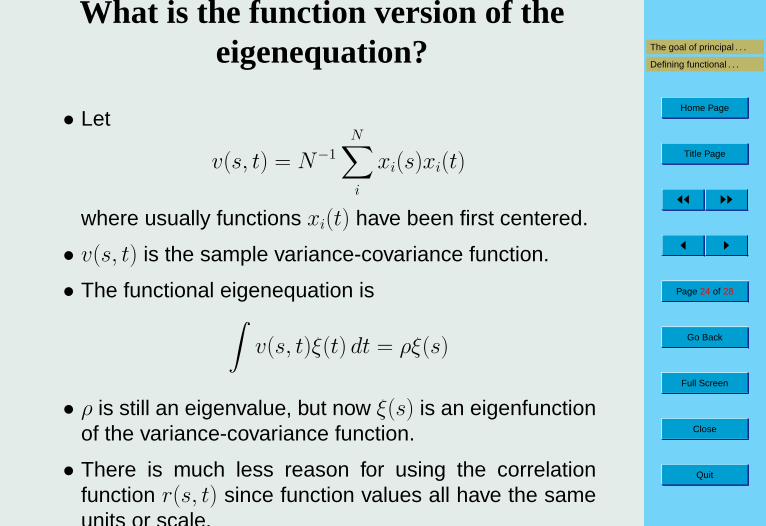
What is the function version of theeigenequation?
• Let
v(s, t) = N−1N∑i
xi(s)xi(t)
where usually functions xi(t) have been first centered.
• v(s, t) is the sample variance-covariance function.
• The functional eigenequation is∫v(s, t)ξ(t) dt = ρξ(s)
• ρ is still an eigenvalue, but now ξ(s) is an eigenfunctionof the variance-covariance function.
• There is much less reason for using the correlationfunction r(s, t) since function values all have the sameunits or scale.

The goal of principal . . .
Defining functional . . .
Home Page
Title Page
JJ II
J I
Page 25 of 28
Go Back
Full Screen
Close
Quit
How do we solve for pairs ofeigenvalues and eigenfunctions?
• Suppose that the observed functions are expanded interms of a vector φ(t) of K basis functions
x(t) = Cφ(t)
• and the jth eigenfunction the expansion
ξj(s) = b′jφ(s) .
• Substituting these expansions into the equation forv(s, t) gives us
v(s, t) = N−1φ′(s)C′Cφ(t)

The goal of principal . . .
Defining functional . . .
Home Page
Title Page
JJ II
J I
Page 26 of 28
Go Back
Full Screen
Close
Quit
• The eigenequation becomes
N−1φ′(s)C′C
∫φ(t)φ′(t) dt bj = ρφ′(s)bj
• Define order K matrix
J =
∫φ(t)φ′(t) dt
so that the eigenequation is now
N−1φ′(s)C′CJbj = ρφ′(s)bj
• This equation has to be true for all argument values s,and consequently,
N−1C′CJbj = ρbj
• subject to the constraint ‖ξ‖2 = 1, which becomes
b′Jb = 1 .

The goal of principal . . .
Defining functional . . .
Home Page
Title Page
JJ II
J I
Page 27 of 28
Go Back
Full Screen
Close
Quit
• if we defineuj = J1/2bj
• then we have the symmetric eigenequation
N−1J1/2C′CJ1/2uj = ρuj
subject to the constraint
u′juj = 1
• We can then use standard software to solve for theeigenvectors uj and back–solve to get the required co-efficient vectors
bj = J−1/2uj
for computing the eigenfunctions ξj(s).
The goal of principal . . .
Defining functional . . .
Home Page
Title Page
JJ II
J I
Page 28 of 28
Go Back
Full Screen
Close
Quit
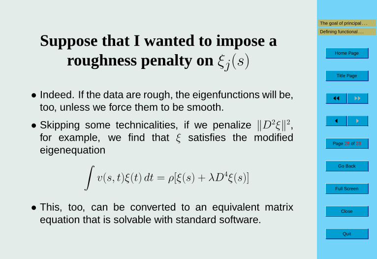
Suppose that I wanted to impose aroughness penalty onξj(s)
• Indeed. If the data are rough, the eigenfunctions will be,too, unless we force them to be smooth.
• Skipping some technicalities, if we penalize ‖D2ξ‖2,for example, we find that ξ satisfies the modifiedeigenequation∫
v(s, t)ξ(t) dt = ρ[ξ(s) + λD4ξ(s)]
• This, too, can be converted to an equivalent matrixequation that is solvable with standard software.