homework 6 spring 2019 aere331 formal due 4/25(s) 10pm
TRANSCRIPT

1
Homework 6 Spring 2019 AerE331 Formal Due 4/25(S) 10pm SOLUTION
Note: The latest possible due date is 5/1(F) 5pm.
PROBLEM 1(20pts) In this problem we will look more closely at Example 3.1 in the Lecture 23 notes. The code
associated with Figure E3.2 is given in the Appendix. Note that the chosen sampling frequency is 60 times the BW of
( )G s . This is twice the authors’ recommended ratio.
(a)(5pts) Obtain a plot of the overlaid step responses for ( )G s ,
( )G z , and ˆ ( )G s . Then comment on the accuracy of ˆ ( )G s
Solution: [See code @ 1(a).]
Comment: The static gain is ~5% high, and as it settles out, it as a
bit of waviness.
Figure(1a) Step Responses for ( )G s , ( )G z , and ˆ ( )G s .
(b)(5pts) Repeat (a), but for max 100sec.t
Solution: [See code @ 1(a).]
Comment: The waviness increases and the trajectory begins to
notably deviate from the expected steady state value.
Figure(1b) Step Responses for ( )G s , ( )G z , and ˆ ( )G s .
(c)(10pts) You should have observed some disturbing behavior
related to ˆ ( )G s in (b). In Example 1 of the Lecture 24 notes there
is a discussion (and code) related to a Pade expansion of the
quantity 1 sTz e
. Repeat (c) using this approximation. In
doing so, not that this quantity appears in both ( )ZOH s and
( )G z
Solution: [See code @ 1(c).] Comment: The offset in static gain
persists, but the waviness and trajectory behavior are gone.
Figure(1c) Step Responses for ( )G s , ( )G z , and ˆ ( )G s .
Remark 1. The purpose of this problem was to highlight the fact that when you periodically extend ( )G z that Matlab
defines for frequenciesN N , what it actually is in continuous-time, the quantity 1 sTz e
has numerical instability
as t . A Pade expansion can be used to remove this instability. If it is not used, simulations could be a nightmare.

2
PROBLEM 2(40pts) In this problem we will address replacement of an analog lead controller by a digital one. In the
Lecture 24 notes we have:
Example 1 This example concerns PROBLEM 3 of HOMEWORK 2. The beginning of that problem states the following:
The Root Locus-based pole placement method was used to design a unity-feedback control system for the plant
)2(
10)(
sssGp
. The result was a lead controller 55.9
)75.2(13.4)(
s
ssGc
. The resulting OL and CL transfer functions are:
)55.9)(2(
)75.2(3.41)()()(
sss
ssGsGsG pc
and 57.1134.6055.11
57.1133.41)(
23
sss
ssW .
In this example, the goal is to replace 55.9
)75.2(13.4)(
s
ssGc
by a suitable ( )cG z .
(a)(10pts) Code related to the code in the example is included in the
Appendix. In it, I have defined the continuous-time transfer function
that approximates the analog controller ( )cG s as ( )ˆ ( ) ( ) ( )p
c cG s G z ZOH s
,
where ( ) ( )p
cG z is the periodic extension of ( )G z that Matlab defines for
frequenciesN N . Obtain overlaid Bode plots for ( )cG s , ( )cG z ,
and ˆ ( )cG s . NOTE: Use the zoom to obtain plots where the magnitude
ranges between roughly -10dB and 20dB, and where the frequency
goes up to onlyN . Then comment on how ˆ ( )cG s compares to ( )cG s .
Solution: [See code @ 2(a).] Figure 2(a) Bode plots for ( )cG s , ( )cG z , and ˆ ( )cG s .
Comment: The magnitude of ˆ ( )cG s approximates that of ( )cG s up until very near N . The phase approximation begins to
break down much earlier, and goes to a lower limit of -90o.
(b)(10pts) Obtain overlaid Bode plots for the OL transfer
functions ( )G s and ˆ ( )G s up toN . Then use the data cursor to compare
the associated CL PMs.
Solution: [See code @ 2(b).]
[ ( )] 180 124 56o o oPM G s and ˆ[ ( )] 180 127 53o o oPM G s .
They compare very well.
Figure 2(b) Bode plots for ( )G s and ˆ ( )G s .

3
(c)(10pts) Obtain overlaid Bode plots for the CL transfer
functions ( )W s and ˆ ( )W s up toN . Then comment on how they
compare, and whether their difference should raise any flags.
Solution: [See code @ 2(c).]
The magnitude of ˆ ( )W s drops below that of ( )W s at very high
frequencies. However, the values are in the range of -60dB,
and so the differences would be negligible. The phase
difference begins to become notable at -20dB. This is not so
small that its influence should be ignored.
Figure 2(c) Bode plots for ( )W s and ˆ ( )W s .
(d)(10pts) Obtain overlaid plots of (i) the impulse responses and (ii) the step responses for ( )W s and ˆ ( )W s . Then comment
how differences between them in each case are connected to the differences you found in (c).
Solution:
The difference in both types of
responses is mainly one of
phase. Hence, it is likely that the
phase difference discussed in (c)
is responsible.
Figure 2(d) Overlaid impulse (LEFT) and step (RIGHT) responses for ( )W s and ˆ ( )W s .
(e)(+5pts) Change the sampling period from 0.05sec.T to 0.01sec.T and repeat (d).
Solution:
The change had a major impact
on both responses. The
approximations are far more
accurate.
Figure 2(d) Overlaid impulse (LEFT) and step (RIGHT) responses for ( )W s and ˆ ( )W s .
4
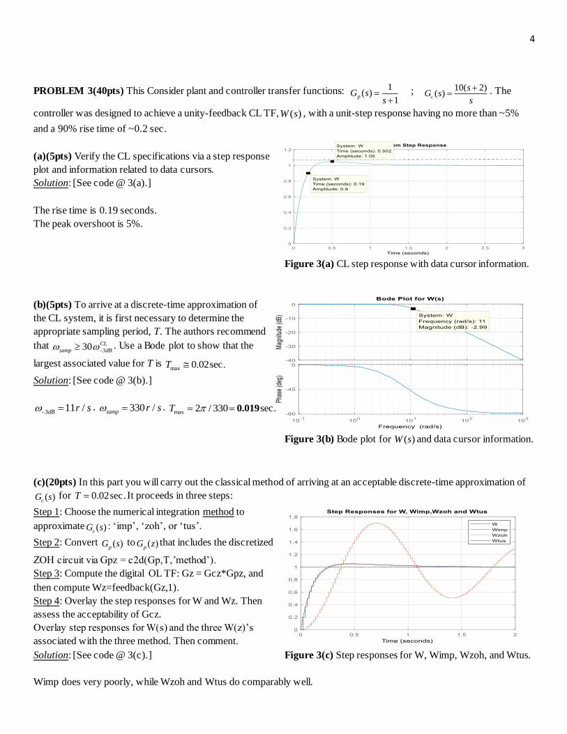
PROBLEM 3(40pts) This Consider plant and controller transfer functions: 1( )
1pG s
s
; 10( 2)
( )c
sG s
s
. The
controller was designed to achieve a unity-feedback CL TF, ( )W s , with a unit-step response having no more than ~5%
and a 90% rise time of ~0.2 sec.
(a)(5pts) Verify the CL specifications via a step response
plot and information related to data cursors.
Solution: [See code @ 3(a).]
The rise time is 0.19 seconds.
The peak overshoot is 5%.
Figure 3(a) CL step response with data cursor information.
(b)(5pts) To arrive at a discrete-time approximation of
the CL system, it is first necessary to determine the
appropriate sampling period, T. The authors recommend
that 330 CL
samp dB . Use a Bode plot to show that the
largest associated value for T is max 0.02sec.T
Solution: [See code @ 3(b).]
3 11 /dB r s . 330 /samp r s . max 2 / 330 sec.T 0.019
Figure 3(b) Bode plot for ( )W s and data cursor information.
(c)(20pts) In this part you will carry out the classical method of arriving at an acceptable discrete-time approximation of
( )cG s for 0.02sec.T It proceeds in three steps:
Step 1: Choose the numerical integration method to
approximate ( )cG s : ‘imp’, ‘zoh’, or ‘tus’.
Step 2: Convert ( )pG s to ( )pG z that includes the discretized
ZOH circuit via Gpz = c2d(Gp,T,’method’).
Step 3: Compute the digital OL TF: Gz = Gcz*Gpz, and
then compute Wz=feedback(Gz,1).
Step 4: Overlay the step responses for W and Wz. Then
assess the acceptability of Gcz.
Overlay step responses for W(s) and the three W(z)’s
associated with the three method. Then comment.
Solution: [See code @ 3(c).] Figure 3(c) Step responses for W, Wimp, Wzoh, and Wtus.
Wimp does very poorly, while Wzoh and Wtus do comparably well.
5
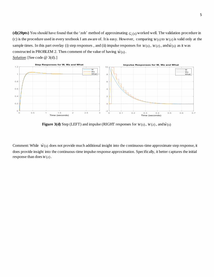
(d)(20pts) You should have found that the ‘zoh’ method of approximating ( )cG s worked well. The validation procedure in
(c) is the procedure used in every textbook I am aware of. It is easy. However, comparing ( )W s to ( )W z is valid only at the
sample times. In this part overlay (i) step responses , and (ii) impulse responses for ( )W s , ( )W z , and ˆ ( )W s as it was
constructed in PROBLEM 2. Then comment of the value of having ˆ ( )W s .
Solution: [See code @ 3(d).]
Figure 3(d) Step (LEFT) and impulse (RIGHT responses for ( )W s , ( )W z , and ˆ ( )W s
Comment: While ˆ ( )W s does not provide much additional insight into the continuous-time approximate step response, it
does provide insight into the continuous-time impulse response approximation. Specifically, it better captures the initial
response than does ( )W z .
6
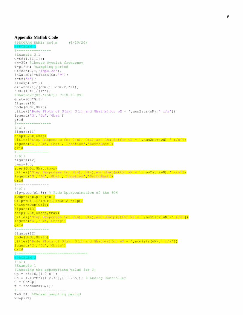
Appendix Matlab Code %PROGRAM NAME: hw6.m (4/20/20)
%PROBLEM 1
%----------------
%Example 3.1
G=tf(1,[1,1]);
wN=30; %Choose Nyquist frequency
T=pi/wN; %Sampling period
Gz=c2d(G,T,'impulse');
[nGz,dGz]=tfdata(Gz,'v');
s=tf('s');
z1=exp(-s*T);
Gz1=nGz(1)/(dGz(1)+dGz(2)*z1);
ZOH=(1-z1)/(T*s);
%Ghat=d2c(Gz,'zoh'); THIS IS BS!
Ghat=ZOH*Gz1;
figure(10)
bode(G,Gz,Ghat)
title(['Bode Plots of G(s), G(z),and Ghat(s)for wN = ',num2str(wN),' r/s'])
legend('G','Gz','Ghat')
grid
%----------------
%(a):
figure(11)
step(G,Gz,Ghat)
title(['Step Responses for G(s), G(z),and Ghat(s)for wN = ',num2str(wN),' r/s'])
legend('G','Gz','Ghat','Location','SouthEast')
grid
%---------------
%(b):
figure(12)
tmax=100;
step(G,Gz,Ghat,tmax)
title(['Step Responses for G(s), G(z),and Ghat(s)for wN = ',num2str(wN),' r/s'])
legend('G','Gz','Ghat','Location','SouthEast')
grid
%---------------
%(c):
z1p=pade(z1,3); % Pade Apprpoximation of the ZOH
ZOHp=(1-z1p)/(T*s);
Gz1p=nGz(1)/(dGz(1)+dGz(2)*z1p);
Ghatp=ZOHp*Gz1p;
figure(13)
step(G,Gz,Ghatp,tmax)
title(['Step Responses for G(s), G(z),and Ghatp(s)for wN = ',num2str(wN),' r/s'])
legend('G','Gz','Ghatp')
grid
%---------------
figure(12)
bode(G,Gz,Ghatp)
title(['Bode Plots of G(s), G(z),and Ghatp(s)for wN = ',num2str(wN),' r/s'])
legend('G','Gz','Ghatp')
grid
%=================================
%PROBLEM 2
%(a):
%Example 1
%Choosing the appropriate value for T:
Gp = tf(10,[1 2 0]);
Gc = 4.13*tf([1 2.75],[1 9.55]); % Analog Controller
G = Gc*Gp;
W = feedback(G,1);
%-----------------------
T=0.01; %Chosen sampling period
wN=pi/T;
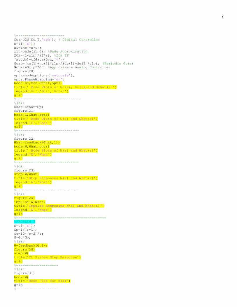
7
%-----------------------
Gcz=c2d(Gc,T,'zoh'); % Digital Controller
s=tf('s');
z1=exp(-s*T);
z1p=pade(z1,3); %Pade Approximation
ZOH=(1-z1p)/(T*s); %ZOH TF
[nc,dc]=tfdata(Gcz,'v');
Gczp=(nc(1)+nc(2)*z1p)/(dc(1)+dc(2)*z1p); %Periodic Gc(z)
Gchat=Gczp*ZOH; %Approximate Analog Controller
figure(20)
opts=bodeoptions('cstprefs');
opts.PhaseWrapping='on';
bode(Gc,Gcz,Gchat,opts)
title(' Bode Plots of Gc(s), Gc(z),and Gchat(s)')
legend('Gc','Gcz','Gchat')
grid
%-------------------------------
%(b):
Ghat=Gchat*Gp;
figure(21)
bode(G,Ghat,opts)
title(' Bode Plots of G(s) and Ghat(s)')
legend('G','Ghat')
grid
%------------------------------
%(c):
figure(22)
What=feedback(Ghat,1);
bode(W,What,opts)
title(' Bode Plots of W(s) and What(s)')
legend('W','What')
grid
%------------------------------
%(d):
figure(23)
step(W,What)
title('Step Responses W(s) and What(s)')
legend('W','What')
grid
%------------------------------
%(e):
figure(24)
impulse(W,What)
title('Impulse Responses W(s) and What(s)')
legend('W','What')
grid
%===========================================
%PROBLEM 3
s=tf('s');
Gp=1/(s+1);
Gc=10*(s+2)/s;
G=Gc*Gp;
%(a):
W=feedback(G,1);
figure(30)
step(W)
title('CL System Step Response')
grid
%--------------------
%(b):
figure(31)
bode(W)
title('Bode Plot for W(s)')
grid
%--------------------
8
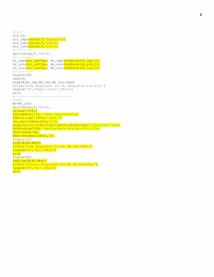
%(c):
T=0.02;
Gcz_imp=c2d(Gc,T,'impulse');
Gcz_zoh=c2d(Gc,T,'zoh');
Gcz_tus=c2d(Gc,T,'tus');
%----------
Gpz=c2d(Gp,T,'zoh');
%----------
Gz_imp=Gcz_imp*Gpz; Wz_imp=feedback(Gz_imp,1);
Gz_zoh=Gcz_zoh*Gpz; Wz_zoh=feedback(Gz_zoh,1);
Gz_tus=Gcz_tus*Gpz; Wz_tus=feedback(Gz_tus,1);
%----------
figure(32)
tmax=2;
step(W,Wz_imp,Wz_zoh,Wz_tus,tmax)
title('Step Responses for W, Wimp,Wzoh and Wtus')
legend('W','Wimp','Wzoh','Wtus')
grid
%------------------------------
%(d):
Wz=Wz_zoh;
Gcz=c2d(Gc,T,'zoh');
z1=exp(-s*T);
z1p=pade(z1,3); %Pade Approximation
ZOH=(1-z1p)/(T*s); %ZOH TF
[nc,dc]=tfdata(Gcz,'v');
Gczp=(nc(1)+nc(2)*z1p)/(dc(1)+dc(2)*z1p); %Periodic Gc(z)
Gchat=Gczp*ZOH; %Approximate Analog Controller
Ghat=Gchat*Gp;
What=feedback(Ghat,1);
figure(33)
step(W,Wz,What)
title('Step Responses for W, Wz and What')
legend('W','Wz','What')
grid
figure(34)
impulse(W,Wz,What)
title('Impulse Responses for W, Wz and What')
legend('W','Wz','What')
grid