homework solutions fall 1996 - user page server for...

Solutions

57:022 HW#1 2/1/97 page 1

57:022 Principles of Design IIHomework Solutions Fall 1996

Dennis L BrickerDept. of Industrial Engineering

University of Iowa

•••••••••••••••••••••••••••• Homework # 1 ••••••••••••••••••••••••••••••••1. A telephone exchange contains 6 lines. A line can be busy or available

for calls and all lines act independently. Each line is busy 75% of thenoon period (so that the probability that a line will be busy at any giventime during the noon period is 75%).a. What is the probability of there being at least three free lines at any

given time during this period? Sol’n: The number N6 of free lines at any given time will have thebinomial distibution with parameter n=6 and p=0.25, i.e., each of thesix lines corresponds to a “trial”, with the line being free correspondingto “success”. Therefore

P N6 ≥ 3{ } =

6

i

0.25( )i 1 − 0.25( )6− i

i =3

6

∑ = 0.1694

b. What is the expected number of free lines at any time during thisperiod?Sol’n: The mean (expected value) of a random variable having abinomial distribution is np, which in this instance is 6(0.25) =1.5

c. You need to make three calls to this exchange, and each time youreceive a busy signal you try again. What is the probability that yourequire exactly six tries in order to complete your three calls?Sol’n: Consider each call to the exchange to be a Bernouilli “trial”, andTk the number of the call on which you receive a free line for the kthtime. Then Tk has a Pascal Distribution (or, for the special case of k=1,a geometric distribution). The required probability is therefore

P T3 = 6{ } =

6 −1

3−1

0.25( )3 1 − 0.25( )6− 3

= 0.1318 + 0.0326 + 0.0044 + 0.0002= 0.0659

2. The foreman of a casting section in a certain factory finds that on theaverage, 1 in every 8 castings made is defective.

N10 = # defects in 10 castings.N10 has the Binomial Distribution with parameters n=10 and

p=1/8.

Solutions

57:022 HW#1 2/1/97 page 2

a. If the section makes 10 castings a day, what is the probability thatnone of these will be defective?Sol’n: Applying the formula for the binomial distribution, we obtain

P N10 = 0{ } =

10

0

1

8

0

1−18

10−0

= 0.2631

b. If the section makes 10 castings a day, what is the probability thattwo of these will be defective?Sol’n: According to the same formula used in (a),

P N10 = 2{ } =

10

2

1

8

2

1−18

10− 2

= 0.2416

c. What is the probability that 3 or more defective castings are made inone day?

Sol’n: P N10 ≥ 3{ } = P N10 = i{ }

i =3

10

∑ = 1− P N10 < 3{ }= 1 - [0.2631+0.3758+0.2416]= 0.1195

3. A light bulb in an apartment entrance fails randomly, with an expectedlifetime of 20 days, and is replaced immediately by the custodian. Assumethat this bulb's lifetime has an exponential distribution.

a. What is the probability that a bulb lasts longer than its expectedlifetime?

Sol’n: T1, the lifetime of the first bulb (i.e., the time of the firstfailure), has exponential distribution with parameters λ =1 failure/20days, i.e., the failure rate is 0.05 failures/day.

P T1 > 20{ } = e− 1

20( ) 20( )= 0.3679

b. If the current bulb was inserted 10 days ago, what is the probabilitythat its lifetime (since it was inserted) will exceed the expectedlifetime of 20 days?Sol’n: Because of the Memoryless Property of the exponentialdistribution, the time between the 10th day and the failure again hasthe same exponential distribution as T1. Therefore, since theprobability that the time from day 10 until the failure will exceed tendays is

P T1 > 10{ } = e− 1

20( ) 10( )= 0.6065 ,

the probability that the total lifetime will exceed 20 days, given that itis at least 10 days, is 60.65%.

c. If you were to test 10 of these bulbs, what is the probability thatmore than half will exceed the expected lifetime?

Solutions

57:022 HW#1 2/1/97 page 3

Sol’n: Consider the testing of each bulb to be a Bernouilli trial, with"success" corresponding to the bulb's exceeding the expected lifetimeof 20 days. Then the number of "successes" in the 10 trials will havethe binomial Distribution with parameters n=10 and p=0.3679 (fromthe answer in (a)).

P N10 >5{ } = P N10 = 6{ } +⋅ ⋅ ⋅ ⋅ ⋅ ⋅+P N10 = 10{ }= 0.083126 + 0.02765 + 0.00603 + 0.00078 + 0.00004= 0.11763

d. If the custodian has 2 spare bulbs, what is the probability that these(including the one currently in use) will be sufficient for the next 60days? Sol’n: Consider the Poisson process in which an event is defined to bea failure of a bulb. Then the number of events during a 60-day periodwill have the Poisson Distribution with rate λ =1 event per 20 days,i.e., 1/20 = 0.05 events/day. The two spare bulbs will be sufficient forthe next 60 days, provided that the number of bulb failures is notgreater than 3. According to the formula for the Poisson distributionwith λ = 0.05 events/day and t=60 days is

P N60 ≤ 3{ } = 0.6472•••••••••••••••••••••••••••• Homework # 2 ••••••••••••••••••••••••••••••••

up a hitchhiker is p=4%, i.e, an average of one in twenty-five drivers will stop;different drivers, of course, make their decisions whether to stop or notindependently of each other.

1. Each car may be considered as a "trial" in a Bernouilli process, with "success"defined as the car's stopping to pick up the hitchhiker.

2. Given that a hitchhiker has counted 15 cars passing him without stopping, whatis the probability that he will be picked up by the 25th car or before?

Soln: Let Z1 = the number of the Bernouilli trial in which “success”first occurs, where p=0.04. Z1 has the geometric distribution, andbecause the Bernouilli process is “memoryless”, we want theprobability that success occurs on or before the 10th trial, i.e.,

P Z1 ≤ 10{ } = P Z1 = n{ }

n =1

10

∑ = (1− p )n −1

n =1

10

∑ p

= 0.04 0.960 + 0.961 + 0.962+......+0.969( ) =0.33517

Solutions

57:022 HW#1 2/1/97 page 4

Suppose that the arrivals of the cars form a Poisson process, at the average rate of 15per minute. Define "success" for the hitchhiker to occur at time t provided that bothan arrival occurs at t and that car stops to pick him up. Let Y1 be the time (inseconds) of the first "success", i.e., the time that he finally gets a ride, when hebegins his wait at time t =0.

3. What is the arrival rate of "successes"? _____0.6______

Soln: Arrival rate of "successes" λ = ( ′ λ ) ⋅( p) = (15) ⋅(0.04) = 0.6

(since the arrivals of the cars form a Poisson process at the averagerate of 15/min. and each of these cars have probability p =0.04 that

it will pick up a hitchhiker.)

4. What is the name of the probability distribution of Y1? Exponential

5. What is the value of E(Y1) ?___1.6667__

Soln: The mean of Exponential Distribution is 1

λ=

1

0.6

6.What's the value of Var(Y1)?___2.7778___

Soln: The variance of Exponential Distribution is 1

λ2 =1

(0.6)2

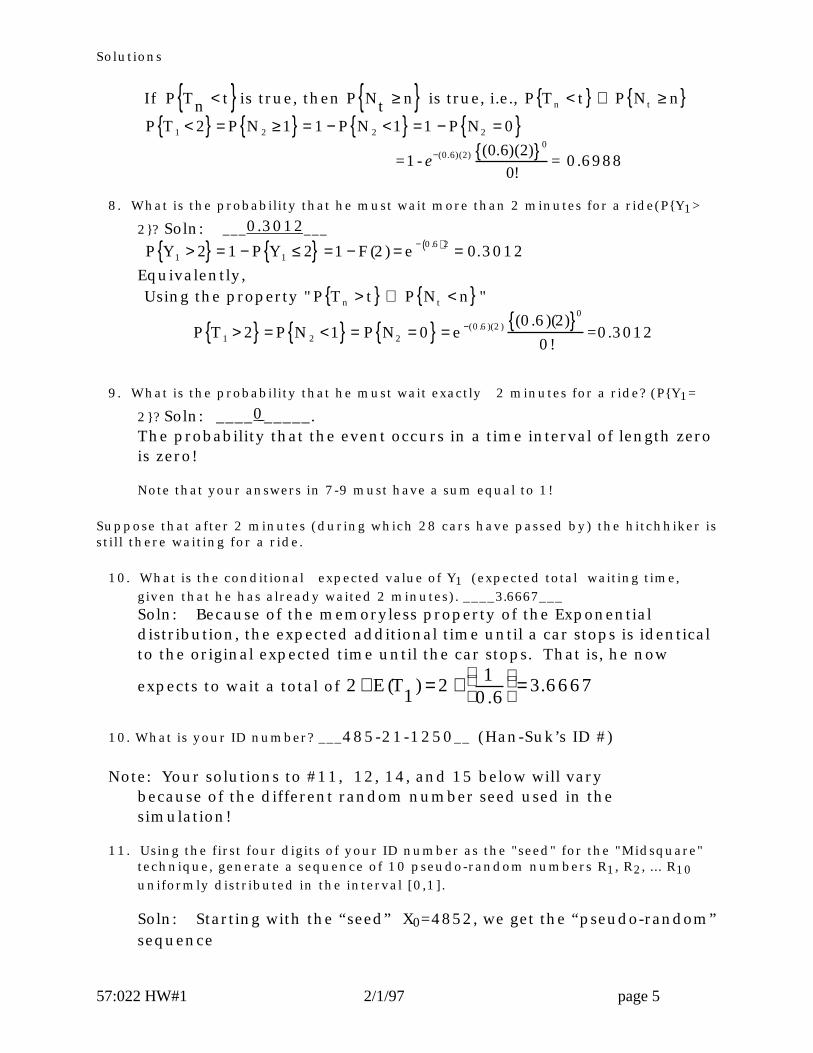
7. What is the probability that he must wait less than 2 minutes for a ride (P{Y1<

2}? ___0.6988__ Soln: The CDF (cumulative distribution function) for Y1, which hasthe exponential distribution, is

F(t) = P Y1 ≤t{ } =1 −e− λt where λ = 0.6.

Another equivalent approach:

Solutions

57:022 HW#1 2/1/97 page 5

If P Tn < t{ } is true, then

P Nt ≥ n{ } is true, i.e., P Tn < t{ } ⇒ P Nt ≥ n{ }

P T1 < 2{ } = P N2 ≥1{ } = 1− P N2 <1{ } =1 − P N2 = 0{ }=1-e−(0.6)(2) (0.6)(2){ }0

0!= 0.6988

8. What is the probability that he must wait more than 2 minutes for a ride(P{Y1>

2}? Soln: ___0.3012___

P Y1 > 2{ } = 1− P Y1 ≤ 2{ } =1− F (2) = e− 0.6( )2 = 0.3012Equivalently,Using the property " P Tn > t{ } ⇔ P Nt < n{ }"

P T1 > 2{ } = P N2 <1{ } = P N2 = 0{ } = e−(0.6)(2) (0.6)(2){ }0

0!=0.3012

9. What is the probability that he must wait exactly 2 minutes for a ride? (P{Y1=

2}? Soln: ____0_____. The probability that the event occurs in a time interval of length zerois zero!

Note that your answers in 7-9 must have a sum equal to 1!

Suppose that after 2 minutes (during which 28 cars have passed by) the hitchhiker isstill there waiting for a ride.

10. What is the conditional expected value of Y1 (expected total waiting time,given that he has already waited 2 minutes). ____3.6667___Soln: Because of the memoryless property of the Exponentialdistribution, the expected additional time until a car stops is identicalto the original expected time until the car stops. That is, he now

expects to wait a total of 2+ E (T1) = 2+ 1

0.6

= 3.6667

10. What is your ID number? ___485-21-1250__ (Han-Suk’s ID #)

Note: Your solutions to #11, 12, 14, and 15 below will varybecause of the different random number seed used in thesimulation!

11. Using the first four digits of your ID number as the "seed" for the "Midsquare"technique, generate a sequence of 10 pseudo-random numbers R1, R2, ... R10uniformly distributed in the interval [0,1].

Soln: Starting with the “seed” X0=4852, we get the “pseudo-random”sequence

Solutions

57:022 HW#1 2/1/97 page 6

i Xi Xi2 Ri

1 4852 23541904 0.54192 5419 29365561 0.36553 3655 13359025 0.35904 3590 12888100 0.88815 8881 78872161 0.87216 8721 76055841 0.05587 0558 00311364 0.31138 3113 09690769 0.69079 6907 47706649 0.7066

10 7066 49928356 0.9283

12. Using the "Inverse Transformation" technique and the 10 numbers generated in(10.), generate the interarrival times τ1, τ2, ... τ10 for the first ten cars with

arrival rate λ = 15/minute, and then the arrival times T1, T2, ... T10 of those tencars.Soln:

i Ri τ i Ti

1 0.5419 0.05204452 0.052044522 0.3655 0.03032787 0.082372383 0.3590 0.02964839 0.112020774 0.8881 0.14600998 0.258030755 0.8721 0.13710044 0.395131196 0.0558 0.00382782 0.398959017 0.3113 0.02486330 0.423822318 0.6907 0.07822957 0.502051889 0.7066 0.08174789 0.58379978

10 0.9283 0.17568430 0.75948408

( Since τi = −

ln R i

λ = −ln 1− R

i

λ , where τi is the inter arrival time,

i.e., τ1 =T1, τ2 = T2 - T1, τ3 = T3 - T2, etc., so that the arrival times areT1=τ1, T2=τ1 + τ2, T3=τ1+ τ2 + τ3, etc.)

13. What is the expected number of arrivals during the first 20 seconds?

Soln: E N1/3

= (15 / min)(

13

min) = 5

14. What is the actual # of arrivals during the first 20 seconds of your simulation?

Soln: 4 arrivals in the first 20 seconds. ( Since the 5th arrivaloccurs at 0.3952 minutes which is later than 0.3333 minutes(= 20seconds). )

15. What is the probability that you would observe exactly this number of arrivalsin this Poisson process? 0.1755 .Soln:

Solutions

57:022 HW#1 2/1/97 page 7

P N1/3 = 4{ } = e−(15)(1/ 3) (15)(1 / 3){ }4

4!= e−554

4!= 0.1755

•••••••••••••••••••••••••••• Homework # 3 ••••••••••••••••••••••••••••••••1. Consider again the proposed drive-up bank teller window in the Hypercard Stack

"Intro. to Simulation", but where the arrival rate of customers has increased to20/hour (one every 3 minutes). The SLAM models for two models (one with asingle teller window and the second with two teller windows), together withoutput, appear below.

••••••••••••••• Case A: single teller •••••••••••••••

GEN,BRICKER,BANKTELLERS,9/12/1996,,,,,,,72;LIM,2,1,50;INIT,0,480;NETWORK;

CREATE,EXPON(3.0),,1;QUE(1),0,4,BALK(OVFLO);ACT(1)/1,EXPON(2.0);COLCT,INTVL(1),CUSTOMER_TIME,20/.5/.5;TERM;

OVFLO COLCT,ALL,OVERFLOW;TERM;END;

FIN;

S L A M I I S U M M A R Y R E P O R T

SIMULATION PROJECT BANKTELLERS BY BRICKER DATE 9/12/1996 RUN NUMBER 1 OF 1

CURRENT TIME .4800E+03 STATISTICAL ARRAYS CLEARED AT TIME .0000E+00

During the 480 simulated time units, there were a totalof 158 cars served by the bank teller. The average timein the system for these cars was 5.86 time units with astandard deviation of 5.20 time units and times rangedfrom 0.0345 to 23.5 time units. The distribution fortime in the system is depicted by the histogram generatedby SLAM II. There was a total of 1 observation ofoverflow.

A histogram of the values collected at a COLCT node canbe obtained. This is accomplished by specifying on inputthe number of interior cells, NCEL; the upper limit ofthe first cell, HLOW; and a cell width, HWID, for thehistogram. The number of cells specified, NCEL, each ofwhich will have a width of HWID. Two additional cellswill be added that contain the interval (-∞,HLOW] and(HLOW+NCEL*HWID,∞).

**STATISTICS FOR VARIABLES BASED ON OBSERVATION**

Solutions

57:022 HW#1 2/1/97 page 8

MEAN STANDARD COEFF. OF MINIMUM MAXIMUM NO.OF VALUE DEVIATION VARIATION VALUE VALUE OBS

CUSTOMER_TIME .586E+01 .520E+01 .887E+00 .345E-01 .235E+02 158 OVERFLOW .182E+03 .000E+00 .000E+00 .182E+03 .182E+03 1

The second category of statistics for this example isthe “file statistics”. The statistics for file 1correspond to the cars waiting for service at bankteller window was 1.25 cars, with a standard deviationof 1.473 cars, a maximum of 4 cars waited, and at theend of the simulation there were no cars in the queue.

**FILE STATISTICS**

FILE AVERAGE STANDARD MAXIMUM CURRENT AVERAGE NUMBER LABEL/TYPE LENGTH DEVIATION LENGTH LENGTH WAIT TIME

1 QUEUE 1.250 1.473 4 0 3.797 2 .000 .000 0 0 .000 3 CALENDAR 1.679 .467 3 1 1.729

The last category of statistics for this example is“statistics on service activities”. The first row of serviceactivity statistics corresponds to the server at bank tellerwindow who was busy 67.9 percent of the time. Since thecapacity of the server is one, the values 12.84 and 87.10refer to the maximum length of the server idle period and theserver busy period, respectively.

**SERVICE ACTIVITY STATISTICS**

ACT ACT LABEL OR SER AVERAGE STD CUR AVERAGE MAX IDL MAX BSY ENT NUM START NODE CAP UTIL DEV UTIL BLOCK TME/SER TME/SER CNT

1 QUEUE 1 .679 .47 0 .00 12.84 87.10 158

**HISTOGRAM NUMBER 1**CUSTOMER_TIME

OBS RELA UPPER FREQ FREQ CELL LIM 0 20 40 60 80 100 + + + + + + + + + + + 9 .057 .500E+00 +*** ˆ + 11 .070 .100E+01 +*** C | + 13 .082 .150E+01 +**** C | + 14 .089 .200E+01 +**** C | + 4 .025 .250E+01 +* C | + 8 .051 .300E+01 +*** C | + 9 .057 .350E+01 +*** C | + 2 .013 .400E+01 +* C | + 7 .044 .450E+01 +** C | + 9 .057 .500E+01 +*** C + 4 .025 .550E+01 +* |C + 6 .038 .600E+01 +** | C + 4 .025 .650E+01 +* | C + 5 .032 .700E+01 +** | C + 5 .032 .750E+01 +** | C + 5 .032 .800E+01 +** | C + 5 .032 .850E+01 +** | C +

Solutions

57:022 HW#1 2/1/97 page 9

6 .038 .900E+01 +** | C + 2 .013 .950E+01 +* | C + 4 .025 .100E+02 +* | C + 3 .019 .105E+02 +* | C + 23 .146 INF +******* ˘ C --- + + + + + + + + + + + 158 0 20 40 60 80 100



CUSTOMER_TIME .586E+01 .520E+01 .887E+00 .345E-01 .235E+02 158

••••••••••••••• Case B: two tellers •••••••••••••••

GEN,BRICKER,BANKTELLERS,9/12/1996,,,,,,,72;LIM,2,1,50;INIT,0,480;NETWORK;

CREATE,EXPON(3.0),,1;QUE(1),0,4,BALK(OVFLO);ACT(2)/1,EXPON(2.0);COLCT,INTVL(1),CUSTOMER_TIME,20/.5/.5;TERM;

OVFLO COLCT,ALL,OVERFLOW;TERM;END;

FIN;


SIMULATION PROJECT BANKTELLERS BY BRICKER DATE 9/12/1996 RUN NUMBER 1 OF 1


During the 480 simulated time units, there were a totalof 179 cars served by the bank teller. The average timein the system for these cars was 2.37 time units with astandard deviation of 2.60 time units and times rangedfrom 0.0117 to 23.6 time units. The distribution fortime in the system is depicted by the histogramgenerated by SLAM II.


MEAN STANDARD COEFF. OF MINIMUM MAXIMUM NO.OF VALUE DEVIATION VARIATION VALUE VALUE OBSCUSTOMER_TIME .237E+01 .260E+01 .110E+01 .117E-01 .236E+02 179OVERFLOW NO VALUES RECORDED

The second category of statistics for this example isthe “file statistics”. The statistics for file 1correspond to the cars waiting for service at bankteller window was 0.099 cars, with a standard deviation

Solutions

57:022 HW#1 2/1/97 page 10

of 0.355 cars, a maximum of 4 cars waited, and at theend of the simulation there were no cars in the queue.

**FILE STATISTICS**

FILE AVERAGE STANDARD MAXIMUM CURRENT AVERAGE NUMBER LABEL/TYPE LENGTH DEVIATION LENGTH LENGTH WAIT TIME 1 QUEUE .099 .355 4 0 0.266 2 .000 .000 0 0 .000 3 CALENDAR 1.785 .794 4 1 2.164

The last category of statistics for this example is“statistics on service activities”. The first row ofservice activity statistics corresponds to the serviceactivity at the bank teller window: the averageutilization was 0.785 which is the average number of busyservers. Since there are two servers, the utilization ofeach individual server was 0.785/2 = 39.25%, which meansthat each server was busy an average of 39.25% of theday. Note that since this activity has a capacity of 2,the maximum idle and busy values refer to the number ofservers, instead of the service times.


ACT ACT LABEL OR SER AVERAGE STD CUR AVERAGE MAX IDL MAX BSY ENT NUM START NODE CAP UTIL DEV UTIL BLOCK TME/SER TME/SER CNT 1 QUEUE 2 .785 .79 0 .00 2.00 2.00 179

**HISTOGRAM NUMBER 1**CUSTOMER_TIME

OBS RELA UPPER FREQ FREQ CELL LIM 0 20 40 60 80 100 + + + + + + + + + + + 27 .151 .500E+00 +******** ˆ + 30 .168 .100E+01 +******** C | + 28 .156 .150E+01 +******** C | + 16 .089 .200E+01 +**** C | + 17 .095 .250E+01 +***** C | + 11 .061 .300E+01 +*** C | + 11 .061 .350E+01 +*** C | + 9 .050 .400E+01 +*** C | + 9 .050 .450E+01 +*** C| + 4 .022 .500E+01 +* C + 3 .017 .550E+01 +* |C + 2 .011 .600E+01 +* | C + 2 .011 .650E+01 +* | C + 2 .011 .700E+01 +* | C + 2 .011 .750E+01 +* | C + 1 .006 .800E+01 + | C+ 0 .000 .850E+01 + | C+ 1 .006 .900E+01 + | C+ 1 .006 .950E+01 + | C+ 0 .000 .100E+02 + | C+ 1 .006 .105E+02 + | C+ 2 .011 INF +* ˘ C --- + + + + + + + + + + + 179 0 20 40 60 80 100

Solutions

57:022 HW#1 2/1/97 page 11


MEAN STANDARD COEFF. OF MINIMUM MAXIMUM NO.OF VALUE DEVIATION VARIATION VALUE VALUE OBSCUSTOMER_TIME .237E+01 .260E+01 .110E+01 .117E-01 .236E+02 179

••••••••••••••••••••••••••••••

a. How many cars were unable to enter the queue each day, because the queue wasfilled to capacity?

Case A: 1 Case B: noneb. What fraction of the time was each teller busy each day?

Case A: 67.9 % Case B: 39.25 %c. Estimate the mean (average) time in the system for the customers.

Case A: 5.86 min . Case B: 2.37 min.d. What fraction of the customers spend more than 5 minutes (total of both waiting

and being served) at the bank? Case A: 72/158 = 45.6% Case B: 17/179 = 9.5%

•••••••••••••••••••••••••••• Homework # 4 ••••••••••••••••••••••••••••••••1. The numbers of arrivals during 100 hours of what is believed to be a Poisson

process were recorded. The observed numbers ranged from zero to nine, withfrequencies O0 through O9:

The average number of arrivals was 3.8/hour. We wish to test the "goodness-of-fit"of the assumption that the arrivals correspond to a Poisson process with arrival rate3.8/hour. The first step is to compute the probability of each observed value, 0through 9:

Solutions

57:022 HW#1 2/1/97 page 12

0.1943588

a. What is the value missing above? (That is, the probability that the number ofarrivals is exactly 4.)

e−3.8 3.8( )4

4!= 0.1943588

b. Now, we can compute the expected number of observations of each of thevalues 0 through 9, which we denote by E0 through E9.• What is the expected number of times in which we would observe fourarrivals per hour?Soln: 19.44• Did we observe more or fewer than the expected number?Soln: The observed number (=24) is more than the expected number (=19.44)

c. Complete the table below:

19.43588 20.831190.1943588 1.07179

d. Ignoring the suggestion that cells should be aggregated so that they contain atleast five observations, what is the observed value of

D = Ei-Oi2

EiΣi

?

Solutions

57:022 HW#1 2/1/97 page 13

Soln: 7.8241705e. Keeping in mind that the assumed arrival rate λ=3.8/hour was estimated from

the data, what is the number of "degrees of freedom"? Soln: 8 (=10-1-1) degrees of freedom

f. Using a value of α = 5%, what is the value of the quantity χ5%2

such that D

exceeds χ5%2

with probability 5% (if the assumption is correct that the

arrivals form a Poisson process with arrival rate 3.8/hour)?Soln: 15.507

g. Is the observed value greater than or less than χ5%2

?

Soln: D (=7.82) < χ5%2

(=15.507)

Should we accept or reject the assumption that the arrival process is Poissonwith rate 3.8/hour?Soln: Accept the assumption that the arrival process is Poisson with rate3.8/hour.

~~~~~~~~~~~~~~~~~~~~~~~~~~~~~~~~~~~~~~~~~~~~~~~~~~~~~~~~~~~~~~~~~~~~~~~~2. Consider again the SLAM II example of the garment factory with 50 sewing

machine operators and machines, 54 machines (including 4 backup machines) and3 repairmen. The original system was modeled by the following SLAM statement.Note that the time units are hours, and that the system is simulated for 2000 hours,i.e., 50 weeks of 40 hours each.

GEN,BRICKER,GARMENTFACTORY,9/18/1996,,,,,,,72;LIM,2,,55;INIT,0,2000;NETWORK;Q1 QUE(1),4; ACTIVITY(50)/1,EXPON(157);Q2 QUE(2); ACTIVITY(3)/2,UNFRM(4,10),,Q1; END;FIN;

The output of this SLAM model is


SIMULATION PROJECT GARMENTFACTORY BY BRICKER DATE 9/18/1996 RUN NUMBER 1 OF 1 CURRENT TIME .2000E+04 STATISTICAL ARRAYS CLEARED AT TIME .0000E+00

**FILE STATISTICS**

FILE AVERAGE STANDARD MAXIMUM CURRENT AVERAGE NUMBER LABEL/TYPE LENGTH DEVIATION LENGTH LENGTH WAIT TIME 1 Q1 QUEUE 1.420 1.311 4 0 4.396 2 Q2 QUEUE .802 1.578 11 4 2.473 3 CALENDAR 51.778 1.390 54 50 48.778


Solutions

57:022 HW#1 2/1/97 page 14

ACT ACT LABEL OR SER AVERAGE STD CUR AVERAGE MAX IDL MAX BSY ENT NUM START NODE CAP UTIL DEV UTIL BLOCK TME/SER TME/SER CNT 1 Q1 QUEUE 50 49.542 1.29 47 .00 10.00 50.00 649 2 Q2 QUEUE 3 2.236 .98 3 .00 3.00 3.00 642

~~~~~~~~~~~~~~~~~~~~~~~~~~~~~~~~~~~~~~~~~~~~~~~~~~~~~~~~~~~~~~~~~~~~~~~The modified example, in which the repair of the failed machines is subcontracted ifthere are already two machines in the repair queue, is modeled by the SLAMstatements:

GEN,BRICKER,GARMENTFACTORY,9/18/1996,,,,,,,72;LIM,2,,55;INIT,0,2000;NETWORK;Q1 QUE(1),4; ACTIVITY(50)/1,EXPON(157);Q2 QUE(2),,2,BALK(SUB); ACTIVITY(3)/2,UNFRM(4,10),,Q1;SUB COLCT,BETWEEN,SUBCONTRACT; ACTIVITY,UNFRM(20,30),,Q1; END;FIN;

The output of this SLAM model is


SIMULATION PROJECT GARMENTFACTORY BY BRICKER DATE 9/18/1996 RUN NUMBER 1 OF 1




SUBCONTRACT .527E+02 .729E+02 .138E+01 .881E-01 .262E+03 35

**FILE STATISTICS**

FILE AVERAGE STANDARD MAXIMUM CURRENT AVERAGE NUMBER LABEL/TYPE LENGTH DEVIATION LENGTH LENGTH WAIT TIME

1 Q1 QUEUE 1.488 1.270 4 1 4.694 2 Q2 QUEUE .277 .577 2 0 .926 3 CALENDAR 52.235 1.060 54 53 51.086


ACT ACT LABEL OR SER AVERAGE STD CUR AVERAGE MAX IDL MAX BSY ENT NUM START NODE CAP UTIL DEV UTIL BLOCK TME/SER TME/SER CNT

1 Q1 QUEUE 50 49.706 .83 50 .00 7.00 50.00 633 2 Q2 QUEUE 3 2.082 .98 3 .00 3.00 3.00 594

Solutions

57:022 HW#1 2/1/97 page 15

~~~~~~~~~~~~~~~~~~~~~~~~~~~~~~~~~~~~~~~~~~~~~~~~~~~~~~~~~~~~~~~~~~~~~~~~~~~~~Note: When “between” statistics are collected, the number of observations is thenumber of intervals between arrival of entities, i.e., one less than the number ofarrivals!

Suppose that• the hourly wage of a sewing machine operator (including benefits, etc.) is $15.• the hourly wage of a machine repairman (including benefits, etc.) is $25.• each machine operator (when busy) generates $27.50 per hour of revenue for

the company,• the cost of subcontracting the repair of a machine is $250.

a. What is the annual payroll for machine operators? Soln: $ 30,000 (=2000 × 15 ) per operator; total is 50($30,000) = $1.5 million

b. What is the annual payroll for repairmen?Soln: $ 50,000 (=2000 × 25 ) per repairman; total is 3($50,000) = $150,000

c. What is the average direct cost of repairing a machine in-house?Soln: $ 77.88/ machine =$25(2000/642)

d. How many repairs were subcontracted during the year?Soln: 36 (Since there were 35 observations of the interval between such repairs,the number of the subcontracted repairs is 36.)

e. How frequently were repairs subcontracted?Soln: once every 52.7 hours (from SLAM II output).

f. What is the average length of time that machines wait in the repair queue?Soln: Without subcontracting: 2.473 hoursSoln: With subcontracting: 0.926 hours

g. What is the maximum number of idle machine operators during the year?Soln: Without subcontracting: 10 operatorsSoln: With subcontracting: 7 operators

h. What is the utilization of each repairman, i.e. the % of time busy?Soln: Without subcontracting: 74.5%Soln: With subcontracting: 69.4 %

i.. How many more man-hours of machine operator time per year are utilized whenthe repairs are subcontracted?Soln: 328 hours more ( = 49.706-49.542)× 2000 )

j. How much more revenue per year is earned by the company when repairs aresubcontracted?Soln: With subcontracting : (49.706× 27.5× 2000)-(250× 36) = 2,724,830

Without subcontracting, revenue is (49.542× 27.5× 2000) = 2,724,810 Difference is $20

k. Is the decision to subcontract the repairs cost-effective? That is, will the increasein the company ‘s revenues compensate for the cost of subcontracting?Soln: Yes, but the increase is so negligible that the company should decide basedupon other non-quantifiable factors.

•••••••••••••••••••••••••••• Homework # 5 ••••••••••••••••••••••••••••••••Regression Analysis. Tests on the fuel consumption of a vehicle traveling atdifferent speeds yeilded the following results:

Speed s (mph) 20 30 40 50 60 70 80 90Consumption C (mile/gal.) 11.4 17.9 22.1 25.5 26.1 27.6 29.2 29.8

(Note: the above data is complete fictitious!)

Solutions

57:022 HW#1 2/1/97 page 16

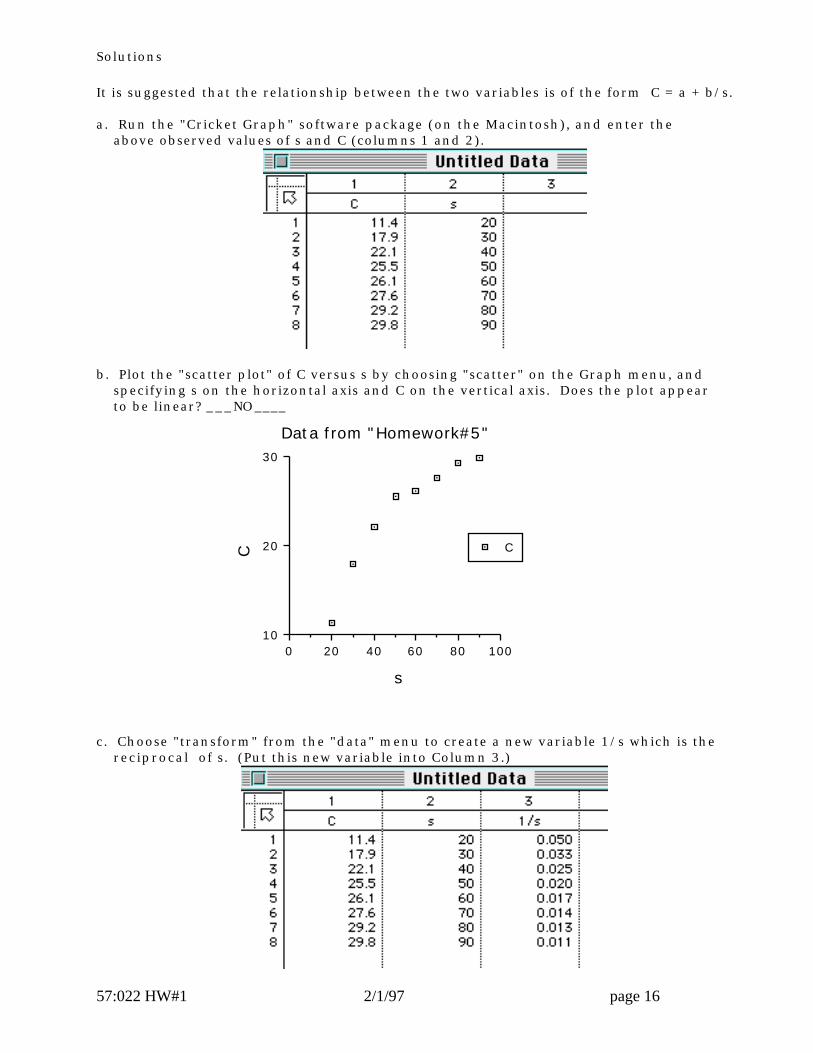
It is suggested that the relationship between the two variables is of the form C = a + b/s.

a. Run the "Cricket Graph" software package (on the Macintosh), and enter theabove observed values of s and C (columns 1 and 2).

b. Plot the "scatter plot" of C versus s by choosing "scatter" on the Graph menu, andspecifying s on the horizontal axis and C on the vertical axis. Does the plot appearto be linear? ___NO____

10080604020010

20

30

C

Data from "Homework#5"

s

C

c. Choose "transform" from the "data" menu to create a new variable 1/s which is thereciprocal of s. (Put this new variable into Column 3.)

Solutions

57:022 HW#1 2/1/97 page 17

d. Plot the "scatter plot" of 1/s (horizontal axis) versus C (vertical axis). Does the plotappear to be linear? ___Yes ____

0.060.050.040.030.020.0110

20

30

C


1/s

C

e. After plotting C versus 1/s, select "Simple" from the "Curve Fit" menu, in order tofit a simple linear relationship between C and 1/s, i.e., to determine a and b such

that C ≈ a + b(1/s). What is the value of a? ___34.604 ___ of b? ___-476.94 ___

Solutions

57:022 HW#1 2/1/97 page 18

476.9434.604

Solutions

57:022 HW#1 2/1/97 page 19

f. Another suggestion is that the relationship is of the form C = axb. Perform theappropriate linear regression to fit a curve of this type. What is the value of a?_2.14067(=e 0.76112 )_ of b? __0.60572 _

54322.4

2.6

2.8

3.0

3.2

3.4

ln C


ln s

ln C

y = 0.76112 + 0.60572x R^2 = 0.923

◊◊◊◊◊◊◊◊◊◊◊◊◊◊◊◊◊◊

Next, start the shareware program “Curve Fit 0.7e ” (author: Kevin Raner) whichcan be found on the “Public Software” fileserver of ICAEN. This program canperform nonlinear regression directly, without first linearizing the function.

g. Enter the values of C and s as before:

2.80000E+01

2.40000E+01

2.00000E+01

1.60000E+01

1.20000E+01

3.00000E+01 6.00000E+01 9.00000E+01

Solutions

57:022 HW#1 2/1/97 page 20

Next, enter the function “f(x) = a + b/x” and give initial values of 1 to theparameters a & b. Then choose “Custom Fn” from the menu in order to find thevalues of a & b which will minimize the sum of the squared errors, using a nonlinearoptimizing algorithm, e.g. a Quasi-Newton algorithm. (You may have encounteredthis type of algorithm, e.g. Fletcher-Powell, in 57:021 “Principles of Design I”.) Besure to indicate that both a & b are to be selected:

Solutions

57:022 HW#1 2/1/97 page 21

h. What is the optimal fitted curve? C = (34.6 ) + (-477 ) / s. What is the SSE (sum ofthe squared errors)? ___2.48990 ___

2.80000E+01

2.40000E+01

2.00000E+01

1.60000E+01

1.20000E+01

3.00000E+01 6.00000E+01 9.00000E+01

a=3.46E+01b=-4.77E+02

Sum of Squares =2.48990

Solutions

57:022 HW#1 2/1/97 page 22

i. Next, enter the power function

and find the optimal curve of this type: C = 3.04 s0.519 . What is the SSE for thisfitted curve? 19.80037

2.80000E+01

2.40000E+01

2.00000E+01

1.60000E+01

1.20000E+01

3.00000E+01 6.00000E+01 9.00000E+01

a=3.04E+00b=5.19E-01

Sum of Squares =19.80037

j. You now have four candidate curves. Write them below, together with their SSE’s.(You may need to compute the values of SSE for the curves fit by Cricket Graphmanually.)

C = asb SSE C = a + b/s SSE-- - - - - - - - - - - - - - - - - - - - - - - - - - - - - - - - - - - - - - - - - - - - - - - - - - - - - - - - - - - - - - - - - - - - - - - - - - - - - - - - - - - - -

Cricket Graph: C = 2.14067s0.60572 25.7847687 C = 34.604 - 476.94 / s 2.48989893

Curve Fit C = 3.04s0.519 19.80037 C = 34.6 - 477 / s 2.48990--- - - - - - - - - - - - - - - - - - - - - - - - - - - - - - - - - - - - - - - - - - - - - - - - - - - - - - - - - - - - - - - - - - - - - - - - - - - - - - - - - - - - -Which one has the smallest SSE?

Soln : The question was perhaps vague, in that “SSE” did not specify in whichequation the error was to be computed, i.e., ln Ci = ln a + b×ln si or Ci = asi

b. Myintention was the latter, i.e., the error in the original curve rather than thelinearized curve.

Solutions

57:022 HW#1 2/1/97 page 23

There is neglible difference between the SSE in the fitted curves of the form C = a +b/s found by Cricket Graph and Curve Fit 0.7e. (This is because the objectivefunctions for the optimization are identical.)

However, this SSE is considerably smaller than that of the two fitted curves of theform C = asb. Note that for the form C = asb, the SSE in the curve found by Curve Fit0.7e is less (19.8 compared to 25.78) than that in the curve found by Cricket Graph.(In these two cases, the objective functions were different, namely

Minimize ln Ci - ln a + b×ln si2∑

i=1

8

in the case of Cricket Graph,

Minimize Ci - as ib 2

∑i=1

8

in the case of Curve Fit 0.7e.

•••••••••••••••••••••••••••• Homework # 6 ••••••••••••••••••••••••••••••••Reasoning that the failure time of a mechanical device is the minimum of the failuretimes of its individual elements (all nonnegative random variables), we willtherefore assume that the failure time of the device has approximately a Weibulldistribution. Suppose that 500 units of this device are operated simultaneously for280 days, at which time 100 have failed, with the failure times:

To estimate the expected lifetime (and its standard deviation) by recording the failuretimes of all 500 units would require perhaps several years, an excessive amount oftime. Hence, we wish to estimate the Weibull parameters u & k from only the dataabove, and use these to estimate µ and σ.

a. Group the observations as follows:Cumulative

Interval # failures # failures % surviving 0- 50 2 2 99.6 50-100 4 6 98.8100-150 15 21 95.8150-200 26 47 90.6200-250 32 79 84.2250-280 21 100 80.0

Solutions

57:022 HW#1 2/1/97 page 24

b. Enter the observed values of t and R (failure time & reliability, i.e., the fractionsurviving) into the Cricket Graph program.

c. Using "transform" on the menu:- compute ln t and place it into column 3 of the data matrix.- compute R-1 and place it into column 4 of the data matrix.- compute ln R-1 and place it into column 5 of the data matrix.- compute ln (ln R-1) and place it into column 6 of the data matrix.

t # of failures

(= NF )

NS FS % Surviving

( = % FS)

5.00E+01 2.00E+00 4.98E+02 9.96E-01 9.96E+01

1.00E+02 6.00E+00 4.94E+02 9.88E-01 9.88E+01

1.50E+02 2.10E+01 4.79E+02 9.58E-01 9.58E+01

2.00E+02 4.70E+01 4.53E+02 9.06E-01 9.06E+01

2.50E+02 7.90E+01 4.21E+02 8.42E-01 8.42E+01

2.80E+02 1.00E+02 4.00E+02 8.00E-01 8.00E+01

t R In t 1/R In (1/R) In ( In(1/R) )

5.00E+01 9.96E-01 3.91E+00 1.00E+00 4.01E-03 -5.52E+00

1.00E+02 9.88E-01 4.61E+00 1.01E+00 1.21E-02 -4.42E+00

1.50E+02 9.58E-01 5.01E+00 1.04E+00 4.29E-02 -3.15E+00

2.00E+02 9.06E-01 5.30E+00 1.10E+00 9.87E-02 -2.32E+00

2.50E+02 8.42E-01 5.52E+00 1.19E+00 1.72E-01 -1.76E+00

2.80E+02 8.00E-01 5.63E+00 1.25E+00 2.23E-01 -1.50E+00

d. Plot the scatter graph of the data, with ln t (column 3) on the horizontal axis,and ln (ln R-1) (column 6) on the vertical axis. Do the points appear to lie on astraight line?

Yes, the points appear to lie on a straight line.

Solutions

57:022 HW#1 2/1/97 page 25

6543-6

-5

-4

-3

-2

-1

ln ( ln (1/R) )

Data from "data.bc"

ln t

ln (

ln (

1/R

) )

e. Fit a line to the points, using the Cricket Graph program. What is the equationof the line? What is its slope and y-intercept?

The Equation is " y = -15.225 + 2.4244 x "

with slope 2.4244 and y-intercept -15.225

6543-6

-5

-4

-3

-2

-1

ln ( ln (1/R) )

Data from "data.bc"

ln t

ln (

ln (

1/R

) )

y = - 15.225 + 2.4244x R^2 = 0.984

Solutions

57:022 HW#1 2/1/97 page 26

f. Based upon the fitted line, what are the parameters u & k of the Weibulldistribution? u = _______________ , k= _______________

k = slope = 2.4244 ≈ 2.4

y-intercept = -k In u = -15.225 ⇒ In u = 6.2799 ⇒ u = e6.2799 = 533.7353

g. According to these values of u & k, what is... the expected lifetime of the device? 473.1563 days... the standard deviation of the device’s lifetime? 210.0341 days... the probability that the device will fail during the first 400 hours is 0.3937

Soln: µY = u ⋅Γ 1 +

1

k

= (533.7353)(0.8865) = 473.1563 = expected lifetime

σY

µY

=Γ 1+

2

k

Γ 2 1 + 1k

−1

⇒

σY

473.1563=

0.9407

0.8865( )2 −1 = 0.4439 ⇒

σY = 210.0341Note: The above evaluations of the Gamma function were done using the tableswhich were e-mailed to the class (& put onto the web site).

F(400) = P{t ≤ 400} = 1 − e−

400

533.7353

2.4

= 0.3937 ∴ 39.37 %

or using the "ProbLib" APL workspace on the macintosh, we can find thatthe expected lifetime of the device is 473.1468,the standard deviation of the device's lifetime is 209.9998, andthe probability that the device will fail during the first 400 hours is 0.3937

h. Using the parameters u & k, compute the expected number of failures (of the100 units tested) in each of the intervals:

Observed Expected Interval # failures # failures

0- 50 ___2___ __1.7__ 50-100 ___4___ __7.2__100-150 __15___ _14.3__150-200 __26____ _22.0__200-250 __32____ _29.55_250-280 __21____ _21.0__

Note: The Weibull cumulative distribution function (CDF) may be evaluatedusing the “ProbLib” APL workspace on the Macintosh, and used to calculate theexpected # of failures in the table above.

Soln: pi = F( ti ) − F( ti−1) ∀ i ≥ 1 , where F( t) = 1− e

− t u( )k

. Thus,

∴ p1 = F( t1) − F(t0 ) = F(50) - F(0) = 1 − e− 50 u( ) k( ) − 1 − e− 0 u( ) k( ) = 0.0034

∴ E1 = 500p1 .= 1.7

p2 = F(t2 ) − F(t1) = F(100) - F(50) = 1 − e− 100 u( ) k( ) − 1 − e− 50 u( )k( ) = 0.0144

∴ E1 = 500p1 .= 7.2

and so on ...

Solutions

57:022 HW#1 2/1/97 page 27

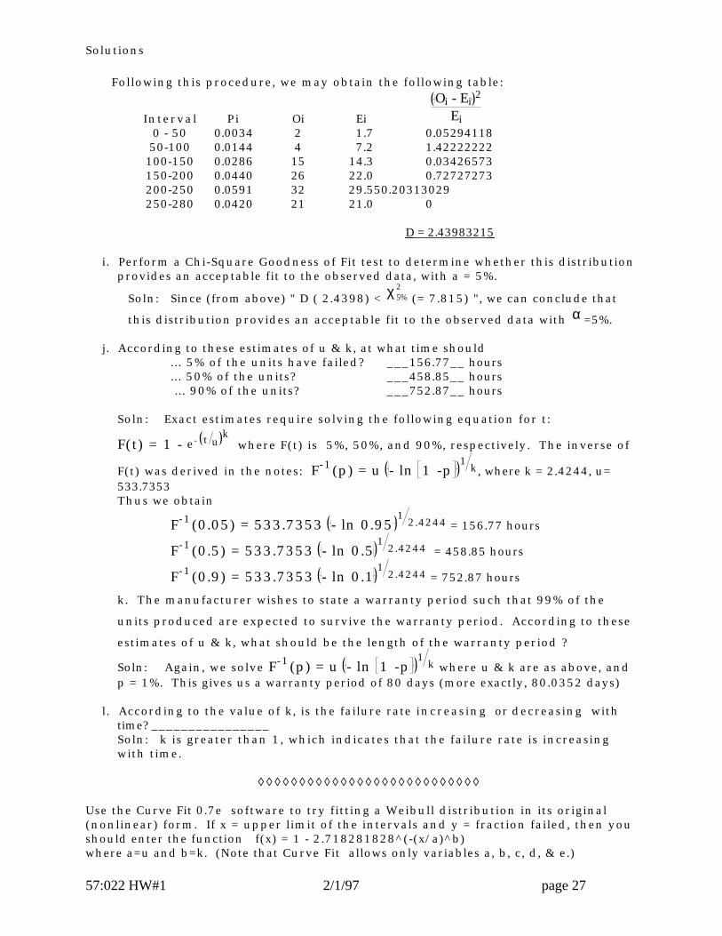
Following this procedure, we may obtain the following table:

Interval Pi Oi Ei

Oi - Ei2

Ei0 - 50 0.0034 2 1.7 0.0529411850-100 0.0144 4 7.2 1.42222222100-150 0.0286 15 14.3 0.03426573150-200 0.0440 26 22.0 0.72727273200-250 0.0591 32 29.550.20313029250-280 0.0420 21 21.0 0

D = 2.43983215

i. Perform a Chi-Square Goodness of Fit test to determine whether this distributionprovides an acceptable fit to the observed data, with a = 5%.

Soln: Since (from above) " D ( 2.4398) < χ 5%2

(= 7.815) ", we can conclude that

this distribution provides an acceptable fit to the observed data with α =5%.

j. According to these estimates of u & k, at what time should... 5% of the units have failed? ___156.77__ hours... 50% of the units? ___458.85__ hours ... 90% of the units? ___752.87__ hours

Soln: Exact estimates require solving the following equation for t:

F(t) = 1 - e- t uk where F(t) is 5%, 50%, and 90%, respectively. The inverse of

F(t) was derived in the notes: F-1(p) = u - ln 1 -p1

k, where k = 2.4244, u=533.7353Thus we obtain

F-1(0.05) = 533.7353 - ln 0.951

2.4244 = 156.77 hours

F-1(0.5) = 533.7353 - ln 0.51

2.4244 = 458.85 hours

F-1(0.9) = 533.7353 - ln 0.11

2.4244 = 752.87 hours

k. The manufacturer wishes to state a warranty period such that 99% of the

units produced are expected to survive the warranty period. According to these

estimates of u & k, what should be the length of the warranty period ?

Soln: Again, we solve F-1(p) = u - ln 1 -p1

k where u & k are as above, andp = 1%. This gives us a warranty period of 80 days (more exactly, 80.0352 days)

l. According to the value of k, is the failure rate increasing or decreasing withtime? ________________Soln: k is greater than 1, which indicates that the failure rate is increasingwith time.

◊ ◊ ◊ ◊ ◊ ◊ ◊ ◊ ◊ ◊ ◊ ◊ ◊ ◊ ◊ ◊ ◊ ◊ ◊ ◊ ◊ ◊ ◊ ◊ ◊ ◊ ◊

Use the Curve Fit 0.7e software to try fitting a Weibull distribution in its original(nonlinear) form. If x = upper limit of the intervals and y = fraction failed, then youshould enter the function f(x) = 1 - 2.718281828^(-(x/a)^b)where a=u and b=k. (Note that Curve Fit allows only variables a, b, c, d, & e.)

Solutions

57:022 HW#1 2/1/97 page 28

m. Using as starting values for a & b the values which you found in (f), try fittingthe curve to the data. What are the values of a & b?

a = _______________ +/- __________________b = _______________ +/- __________________

Was Curve Fit able to find values with small error estimates (e.g. with error lessthan about 5 or 10% of the parameter)? ________If yes, proceed to question (n); otherwise, stop .

Soln: According to the Curve Fit output, the parameters are

a = 533.73486 +/- 23.74058

b = 2.35061 +/- 0.13497

Yes, the Curve fit can find values with small error estimates.

2.00000E-01

1.60000E-01

1.20000E-01

8.00000E-02

4.00000E-02

1.00000E+02 2.00000E+02Corr. Coeff. (R2) = 0.99607Sum of Squares = 0.00013

n. What are the values of the parameters for this new fitted distribution?

u = 534 , k = 2.35

o. According to these values of u & k, what is... the expected lifetime of the device? 473.2137... the standard deviation of the device’s lifetime? 214.0274... the probability that the device will fail during the first 400 hours? 0.3978

Soln: See solution of (g) above.

p. Using these new parameters u & k, compute the expected number of failures (ofthe 100 units tested) in each of the intervals:

Observed Expected Interval # failures # failures 0- 50 ________ _______ 50-100 ________ _______100-150 ________ _______

Solutions

57:022 HW#1 2/1/97 page 29

150-200 ________ _______200-250 ________ _______250-280 ________ _______

Soln: pi = F( ti ) − F( ti−1) ∀ i ≥ 1 , where F( t) = 1− e

− t u( )k

. Thus,

∴ p1 = F( t1) − F(t0 ) = F(50) - F(0) = 1 − e− 50 u( ) k( ) − 1 − e− 0 u( ) k( ) = 0.0038

∴ E1 = 500p1 .= 1.90

p2 = F(t2 ) − F(t1) = F(100) - F(50) = 1 − e− 100 u( ) k( ) − 1 − e− 50 u( )k( ) = 0.0155

∴ E1 = 500p1 = 7.75and so on ...

Following this procedure, we may obtain the following table:

Interval Pi Oi Ei

Oi - Ei2

Ei0 - 50 0.0038 2 1.90 0.0052631650-100 0.0155 4 7.75 1.81451613100-150 0.0300 15 15.00 0150-200 0.0454 26 22.70 0.47973568200-250 0.0600 32 30.00 0.13333333250-280 0.0423 21 21.15 0.00106383

D = 2.43391213

q. According to these new estimates of u & k, at what time should... 5% of the units have failed? 156.84 days... 50% of the units? 459.09 days ... 90% of the units? 753.26 days

Soln: See solution of (j) above.

◊ ◊ ◊ ◊ ◊ ◊ ◊ ◊ ◊ ◊ ◊ ◊ ◊ ◊ ◊ ◊ ◊ ◊ ◊ ◊ ◊ ◊ ◊ ◊ ◊ ◊ ◊

r. You needn’t perform a “goodness-of-fit” test to confirm it, but state youropinion about which Weibull distribution seems to be a better fit.Soln: I f we were to perform the “goodness-of-fit” test, then since " D ( =2.4339)

< χ 5%2

(= 7.815) ", we would conclude that this distribution also provides anacceptable fit to the observed data with α =5%. The results are so similar thatthere is probably no significant difference in the qualities of the fits. If eachprogram found the exact optimum of its objective function, then clearly theresult of Curve Fit would be a better fit. However, because Curve Fit is doingcomputation with nonlinear functions while Cricket Graph is using linearfunctions, the latter will perform the computations more accurately.

•••••••••••••••••••••••••••• Homework # 7 ••••••••••••••••••••••••••••••••1. A system contains 4 types of devices, with the system reliability represented

schematically by

Solutions

57:022 HW#1 2/1/97 page 30

It has been estimated that the lifetime probability distributions of the devices are asfollows:

A: Weibull, with mean 1000 days and standard deviation 1200 daysB: Exponential, with mean 4000 daysC: Normal, with mean 3000 days and standard deviation 750 daysD: Exponential, with mean 1000 days

a.) Compute the reliabity of a unit of each device for a designed system lifetime of 1000 days:

Sol’n: Device Reliability R(1000)

A 33.91% RA(1000) = 1 − FA (1000) = e−

1000

910.6269

0.8376

B 77.88% RB(1000) = 1 − FB(1000) = e− 1000

4000

C 99.62% From CDF table of Normal Distribution

D 36.79% RD(1000) = 1− FD(1000) = e−1000

1000

b.) Using the reliabilities in (a), compute the system reliability:Sol’n:

Subsystem Reliability R(1000) AA 0.5632 % Since 1 − (1− RA )2 = 1 − (1− 0.3391)2

AA+B+C 0.4370 % RAA × RB × RC

B+DDD 0.5821 % RB × RDDD = 0.7788 × 1 − 1− 0.3679( )3{ }Total system: 0.7647 % 1 − (1− RAA × RB × RC)(1− RB × RDDD )

c.) Draw a SLAM network which can simulate the lifetime of this system. (You need notperform the simulation.)

Solutions

57:022 HW#1 2/1/97 page 31

Notes:• The CREATE node indicates that only 1 entity is initially created.• “A”, “B”, “C”, and “D” above should be replaced by the lifetime distribution of the

corresponding devices, i.e., WEIBL( , ), EXPON(4000), RNORM(3000,750), and EXPON(1000),respectively.

• The parameters of the Weibull distribution as defined by SLAM are named ALPHA andBETA, and are not (µ,σ), the mean & standard deviation. ALPHA is identical to the

parameter k in the class notes, and BETA is uk. To determine u and k from the mean andstandard deviation, one may roughly estimate k given the coefficient of variation σ/µ=1.2 from the table below (taken from the class notes):

The value of k is between 0.8 and 0.9; interpolating would give k=0.8 + .1(0.06/0.15) =0.84. Next, the parameter u may be found from

µ = u Γ 1+1k

⇒ u = µ

Γ 1+1k

= 1000

Γ 1+ 10.84

≈ 10001.1

= 909.09

where the Gamma function is evaluated by interpolating in the table below (also foundin the notes):

Solutions

57:022 HW#1 2/1/97 page 32

Thus, “A” in the diagram above should be WEIBL(0.84, 909).• The numbers in the ACCUMULATE nodes are: FR = number of arriving entities required

to cause the first entity to be “released” from the node; SR = number of arrivingentities required for subsequent entities to be “released” from the node.

• In the ACCUMULATE nodes N1, N3, and N5, the value of SR is irrelevant, since FR isassigned a value equal to the total number of arrivals at the node, and no subsequententities will ever be released from the node. (The default value will be 1.)

• In the ACCUMULATE nodes N2 and N4, additional entities may arrive after the first entityis released from the node, and therefore a value of SR (larger than the maximumnumber of entities which might arrive) must be specified. In the diagram above, 9 wasspecified, but any larger and some smaller values are possible.

• The COLCT (COLLECT) node will collect statistics on the time of the FIRST arrival; in thiscase, the “1” on the TERMINATE node cause the simulation to then end, and so nofurther arrivals can occur. For this reason, it would be equivalent to specify INTVL(1)instead of FIRST if you also indicate on the CREATE statement that the creation time (0 inthis case) is to be recorded in attribute #1 (i.e., the parameter MA = 1).

2. A system has 3 types of components (A, B, & C) which are subject to failure. As shownbelow, the system requires at least one of components A and B, and at least two ofcomponent C. One of component A is in “stand-by”. That is, when the first component Ahas failed, the second is to be switched on, and until then does not begin to "age" or fail.Assume that the sensor/switch has 95% reliability. In the case of components B & C, onthe other hand, all units of these components are in operation simultaneously, so thateach unit is subject to failure from the beginning of the system’s operation. Note that thesystem requires at least 2 of component C for proper functioning.

The lifetime distributions of the three component types are:Component A: Erlang, being the sum of five random variables, each

having exponential distribution with mean 100 days.

Solutions

57:022 HW#1 2/1/97 page 33

Component B: Exponential, with expected lifetime 200 days.Component C: Exponential, with expected lifetime 300 days.

a. Draw a SLAM network which can simulate the lifetime of this system.Sol’n:

Notes:• Again, the values “A”, “B”, and “C” on the diagram above should be replaced by

the lifetime distributions, namely ERLNG(100,5), EXPON(200), and EXPON(300),respectively.

• The parameters of the Erlang distribution in SLAM are not the mean andstandard deviation (which would be in this case 500 and

5×1002 = 100 5 = 223.61), but the mean of each of the component exponentialdistributions and the number of such distributions.

• The “1” in the GOON node (labelled N1) indicates that the entity which arrivesthere (at the time of the failure of the primary unit of device A) must leavenode N1 via a single activity only.

• The two activities leaving the GOON node N1 represent (1) the lifetime of thestandby unit of device A, which receives the entity with 99% probability, and(2) the failure of the switch, requiring time = 0, which receives the entity withprobability 1%.

• See the note in problem 1 about the values of the parameters FR and SR of theACCUMULATE nodes.

• See the note in problem 1 about the FIRST statistics collected by the COLCT node.

b. Enter the network into the computer, and simulate the system 1000 times,collecting statistics on the time of system failure. Request that a histogram beprinted. Specify about 15-20 cells, with HLOW and HWID parameters which will giveyou a "nice" histogram with the mean approximately in the center and with smalltails. (This may require a second simulation, with the histogram parameters selectedafter observing the results of a preliminary simulation.)

Note: Be sure to specify on the GEN statement that you do NOT want intermediateresults, and that the SUMMARY report is to be printed only after the 1000th run. Alsospecify on the INITIALIZE statement that the statistical arrays should not be clearedbetween runs. The following should work:GEN,yourname,RELIABILITY,10/16/96,1000,,N,,N,Y/1000,72;LIM,,,8;INIT,,,NO;NETWORK;

Solutions

57:022 HW#1 2/1/97 page 34

(SLAM II network statements go here)END;

FIN;

Sol’n: The (edited) SLAM output appears below:

1 GEN,Hansuk Sohn,Reliability,10/9/1996,1000,,N,,N,Y/1000,72; 2 LIM,,,8; 3 INIT,,,NO; 4 NETWORK; 5 CREATE; 6 ACT/1,ERLNG(100,5),,Na; Component A 7 ACT/2,EXPON(200),,Nb; Component B 8 ACT/3,EXPON(200),,Nb; Component B 9 ACT/4,EXPON(300),,Nc; Component C 10 ACT/5,EXPON(300),,Nc; Component C 11 ACT/6,EXPON(300),,Nc; Component C 12 Na GOON,1; 13 ACT,ERLNG(100,5),0.95,FAIL; 14 ACT,0,0.05,FAIL; 15 Nb ACCUM,2; Node "b" will be released when both Bs fail. 16 ACT,,,FAIL; 17 Nc ACCUM,2; Node "c" will be released when 2 out of 3 Cs fail. 18 ACT,,,FAIL; 19 FAIL COLCT,FIRST,TIME_OF_FAILURE,20/0/20; 20 TERM,1; 21 END; 22 FIN;


SIMULATION PROJECT RELIABILITY BY HANSUK SOHNDATE 10/ 9/1996 RUN NUMBER 1000 OF 1000


**STATISTICS FOR VARIABLES BASED ON OBSERVATION** MEAN STANDARD COEFF. OF MINIMUM MAXIMUM NO.OF VALUE DEVIATION VARIATION VALUE VALUE OBSTIME_OF_FAILURE .174E+03 .116E+03 .669E+00 .224E+01 .666E+03 1000

**REGULAR ACTIVITY STATISTICS** ACTIVITY AVERAGE STANDARD MAXIMUM CURRENT ENTITY INDEX/LABEL UTILIZATION DEVIATION UTIL UTIL COUNT 1 COMPONENT A .1315 .3380 1 1 0 2 COMPONENT B .4178 .4932 1 1 0 3 COMPONENT B .3887 .4874 1 0 1 4 COMPONENT C .3057 .4607 1 1 0 5 COMPONENT C .3012 .4588 1 0 1 6 COMPONENT C .3357 .4722 1 0 1

**HISTOGRAM NUMBER 1**TIME_OF_FAILURE

OBS RELA UPPER FREQ FREQ CELL LIM 0 20 40 60 80 100 + + + + + + + + + + + 0 .000 .000E+00 + + 22 .022 .200E+02 +* +

Solutions

57:022 HW#1 2/1/97 page 35

53 .053 .400E+02 +***C + 73 .073 .600E+02 +**** C + 75 .075 .800E+02 +**** C + 85 .085 .100E+03 +**** C + 84 .084 .120E+03 +**** C + 77 .077 .140E+03 +**** C + 70 .070 .160E+03 +**** C + 62 .062 .180E+03 +*** C + 58 .058 .200E+03 +*** C + 41 .041 .220E+03 +** C + 53 .053 .240E+03 +*** C + 51 .051 .260E+03 +*** C + 35 .035 .280E+03 +** C + 25 .025 .300E+03 +* C + 24 .024 .320E+03 +* C + 22 .022 .340E+03 +* C + 15 .015 .360E+03 +* C + 12 .012 .380E+03 +* C + 11 .011 .400E+03 +* C + 52 .052 INF +*** C --- + + + + + + + + + + + *** 0 20 40 60 80 100


MEAN STANDARD COEFF. OF MINIMUM MAXIMUM NO.OF VALUE DEVIATION VARIATION VALUE VALUE OBSTIME_OF_FAILURE .174E+03 .116E+03 .669E+00 .224E+01 .666E+03 1000

c. What is your estimate of the average lifetime of this system, based upon the simulationresults?Sol’n: 174 days ( from SLAM output )

d. Suppose that the system is required to survive for a 100-day mission. What is theestimated reliability of the system, i.e., the probability that the system survives 100 days?Sol’n: From the histogram above, we see that 308 (the sum of the first six cells) failuresoccurred during the first 100 days (and 1000-308=692 survived at least 100 days). Hence,

R(100) = 1-308

1000 = 0.692

e. Suppose your company will offer a warranty on this system, specifying the length ofthe warranty period such that 98% of the systems will survive past the warranty period.What should be the length of the warranty?

Sol’n: The above histogram doesn’t provide sufficient detail at the low end to allow anaccurate estimate, but if we use a linear interpolation we would estimate that the 20thfailure occurred at time 20(20/22) = 18.2 days, leaving at that time 980 survivors (98% ofthe systems simulated.) Therefore, according to this estimate, 18.2 days should be thelength of the warranty (which undoubtedly would be rounded to 18 days for the sake ofconvenience). Interpolating again to find the reliability of the system for an 18-daylifetime, we would estimate that 22(18/20) = 19.8 systems, or 1.98% of the total, failedduring the first 18 days, leaving 98.02% surviving.

To get a more accurate estimate of the correct warranty period, we should• increase the number of runs from 1000, e.g., to as many as 10000• change the specifications for the histogram so as to get a count of failures each

day, e.g.,

Solutions

57:022 HW#1 2/1/97 page 36

FAIL COLCT,FIRST,TIME_OF_FAILURE,30/0/1;which would give 30 cells, each of length 1 day.

•••••••••••••••••••••••••••• Homework # 8 ••••••••••••••••••••••••••••••••1. Project Scheduling. Consider the home-building project: Predecessor Duration (days)

Activity Description Activities Mean Std DevA Walls & ceiling B 5 2B Foundation none 4 1C Roof timbers A 2 1D Roof sheathing C 2 1E Electrical wiring A 4 2F Roof shingles D 2 1G Exterior siding H 5 1H Windows A 4 1I Paint F,G,J 3 1J Inside wall board E,H 3 1

1. Complete the AON network by labeling the nodes:

J

H G

I

2. Complete the AOA & the corresponding SLAM networks below by inserting any"dummy" activities which are necessary, and labeling the nodes.

3. Give numerical values (0, 1, 2, 3, 4, or ∞ ) for parameters "a" - "i" and a statistictype for “j” on the SLAM network below which would simulate the project andcollect statistics on the completion time. (You needn’t insert the probabilitydistributions for the durations!)

Solutions

57:022 HW#1 2/1/97 page 37

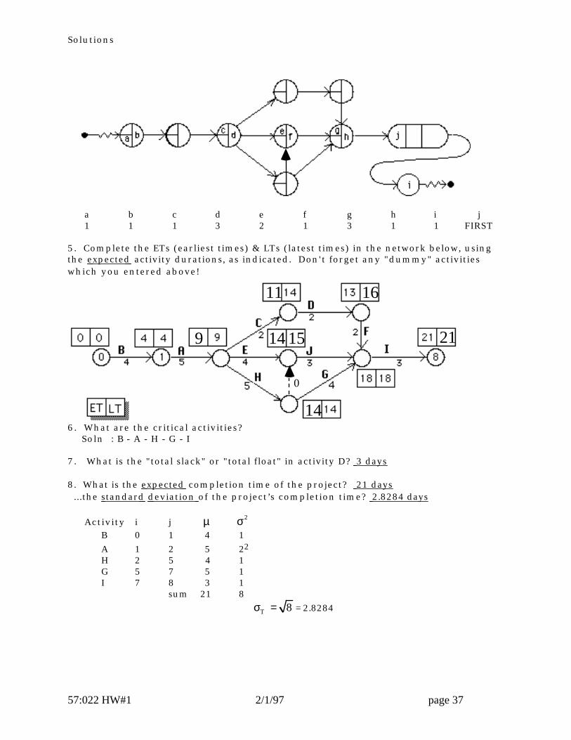
a b c d e f g h i j1 1 1 3 2 1 3 1 1 FIRST

5. Complete the ETs (earliest times) & LTs (latest times) in the network below, usingthe expected activity durations, as indicated. Don't forget any "dummy" activitieswhich you entered above!

9

11

14 15

14

21

16

0

6. What are the critical activities? Soln : B - A - H - G - I

7. What is the "total slack" or "total float" in activity D? 3 days

8. What is the expected completion time of the project? 21 days ...the standard deviation of the project’s completion time? 2.8284 days

Activity i j µ σ2

B 0 1 4 1A 1 2 5 22

H 2 5 4 1G 5 7 5 1I 7 8 3 1

sum 21 8

σT = 8 = 2.8284

Solutions

57:022 HW#1 2/1/97 page 38

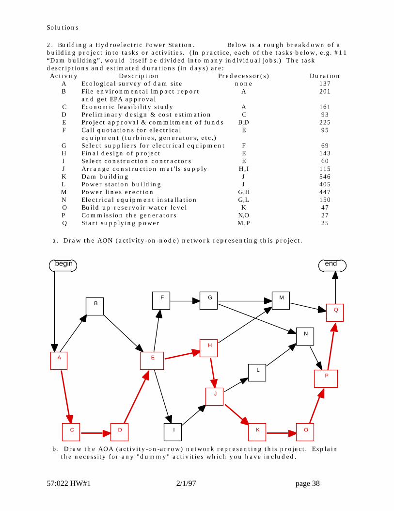
2. Building a Hydroelectric Power Station. Below is a rough breakdown of abuilding project into tasks or activities. (In practice, each of the tasks below, e.g. #11“Dam building”, would itself be divided into many individual jobs.) The taskdescriptions and estimated durations (in days) are:Activity Description Predecessor(s) Duration

A Ecological survey of dam site none 137B File environmental impact report A 201

and get EPA approvalC Economic feasibility study A 161D Preliminary design & cost estimation C 93E Project approval & commitment of funds B,D 225F Call quotations for electrical E 95

equipment (turbines, generators, etc.)G Select suppliers for electrical equipment F 69H Final design of project E 143I Select construction contractors E 60J Arrange construction mat’ls supply H,I 115K Dam building J 546L Power station building J 405M Power lines erection G,H 447N Electrical equipment installation G,L 150O Build up reservoir water level K 47P Commission the generators N,O 27Q Start supplying power M,P 25

a. Draw the AON (activity-on-node) network representing this project.

A

C

B

D

E

F

I

G

H

J

L

K

M

N

O

P

Q

begin end

b. Draw the AOA (activity-on-arrow) network representing this project. Explainthe necessity for any "dummy" activities which you have included.

Solutions

57:022 HW#1 2/1/97 page 39

A

B

C

D

E

F

G

H

I

J K

M

N

O

Q

L

P

c. Label the nodes of the AOA network, so that i<j if there is an activity with node ias its start and node j as its end node.

A

B

C

D

E

F

G

H

I

J K

M

N

O

Q

L

P

0 1

2

3

4

5

6

7

8

9

10

11

12

13

14 15

d. Perform the forward pass through the AOA network to obtain for each node i,ET(i) = earliest possible time for event i.

Solutions

57:022 HW#1 2/1/97 page 40

A

B

C

D

E

F

G

H

I

J K

M

N

O

Q

L

P

0 1

2

3

4

5

6

7

8

9

10

11

12

13

14 15

0 137

15191494780780711

1467

1420874759298

1279759616391

e. What is the earliest completion time for this project? 1519 days

f. Perform the backward pass through the AOA network to obtain, for each node i,LT(i) = latest possible time for event i (assuming the project is to be completed inthe time which you have specified in (e).)

A

B

C

D

E

F

G

H

I

J K

M

N

O

Q

L

P

0 1

2

3

4

5

6

7

8

9

10

11

12

13

14 15

0 137

1519149410471047978

14671317759616391

1420874759298

g. For each activity, compute and record below:ES = earliest start timeLS = latest start timeEF = earliest finish timeLF = latest finish timeTF = total float (slack)

Sol’n:

Solutions

57:022 HW#1 2/1/97 page 41

Critical Activity Activity ES LS EF LF TF Yes A 0 0 137 137 0No B 137 190 338 391 53 Yes C 137 137 298 298 0 Yes D 298 298 391 391 0 Yes E 391 391 616 616 0No F 616 883 711 978 267No G 711 978 780 1047 267 Yes H 616 616 759 759 0No I 616 699 676 759 83 Yes J 759 759 874 874 0 Yes K 874 874 1420 1420 0No L 874 912 1279 1317 38No M 780 1047 1227 1494 267No N 1279 1317 1429 1467 38 Yes O 1420 1420 1467 1467 0 Yes P 1467 1467 1494 1494 0 Yes Q 1494 1494 1519 1519 0

h. Which activities are "critical", i.e., have zero float? (Circle the labels A-Q of thecritical activities above.) Indicate the critical path in your AOA network in part(b).

Soln : A - C - D - E - H - J - K - O - P - Q

A

B

C

D

E

F

G

H

I

J K

M

N

O

Q

L

P

0 1

2

3

4

5

6

7

8

9

10

11

12

13

14 15

i. Schedule this project by entering the AON network into the MacProject PROsoftware Specify that the start time for the project will be November 1, 1996.What is the earliest completion date for the project? August 28, 2002

(Note that• stated to the left and right of each node, i.e., acitivity, are the earliest start and

latest finish dates, respectively.• MacProject PRO assumes 5-day work weeks by default, so that the time between

beginning & completion date isn’t the same as your answer in (e).)

ES EFES : Earliest Start TimeEF : Earliest Finish Time

Solutions

57:022 HW#1 2/1/97 page 42

A

11/1/96 5/12/97

C

5/13/97 12/23/97

B

5/13/97 2/17/98

D

12/24/97 5/1/98

E

5/4/98 3/12/99

F

3/15/99 7/23/99

I

3/15/99 6/4/99

H

3/15/99 9/29/99

G

7/26/99 10/28/99

J

9/30/99 3/8/00

K

3/9/00 4/11/02

L

3/9/00 9/26/01

M

10/29/99 7/16/01

N

9/27/01 4/24/02

O

4/12/02 6/17/02

P

6/18/02 7/24/02

Q

7/25/02 8/28/02

•••••••••••••••••••••••••••• Homework # 9 ••••••••••••••••••••••••••••••••Building a Hydroelectric Power Station. Below is a rough breakdown of abuilding project into tasks or activities. (In practice, each of the tasks below, e.g. K(#11) “Dam building”, would itself be divided into many individual jobs.) The taskdescriptions and estimated durations (in days) are:

Activity Description Predecessor(s) DurationA Ecological survey of dam site none 137 ± 12

B File environmental impact report A 201 ± 18and get EPA approval

C Economic feasibility study A 161 ± 14

D Preliminary design & cost estimation C 93 ± 5

Solutions

57:022 HW#1 2/1/97 page 43

E Project approval & commitment of funds B,D 225 ± 20

F Call quotations for electrical E 95 ± 10equipment (turbines, generators, etc.)

G Select suppliers for electrical equipment F 69 ± 5H Final design of project E 143 ± 12

I Select construction contractors E 60 ± 5J Arrange construction mat’ls supply H,I 115 ± 15

K Dam building J 546 ± 30

L Power station building J 405 ± 25

M Power lines erection G,H 447 ± 15

N Electrical equipment installation G,L 150 ± 10

O Build up reservoir water level K 47 ± 15

P Commission the generators N,O 27 ± 2Q Start supplying power M,P 25 ± 3

(This is the same data as given in Homework #8, except that the durations are nowgiven as intervals centered around the originally-given duration.)

The AOA network representing this project is shown on the next page.

a. Use SLAM to simulate the project 1000 times, with a triangular distribution for theactivity durations, e.g., TRIAG(125,137,149) for activity A. (Note that the meanvalue for each duration is the central value which was used in Homework #8, e.g.,137 days for activity A.)

Warning! In the case of a “dummy” activity with duration 0, or any otherconstant, don’t specify a probability distribution such as TRIAG(0,0,0), whichwould lead to an error message!

Solutions

57:022 HW#1 2/1/97 page 44

Solutions :

l-ecn015% rslam 1a-1

1 GEN,Hansuk Sohn,Hydroelectric Power Station,11/5/1996,1000,,N,,N,Y/1000,72; 2 LIM,20,50,500; 3 INIT,,,NO; 4 NETWORK; 5 CREATE,,,,1; 6 ACT/1,TRIAG(125,137,149),,N1; Activity A +/- 12 7 N1 ACCUM,,,,2; 8 ACT/2,TRIAG(147,161,175),,N2; Activity C +/- 14 9 ACT/3,TRIAG(183,201,219),,N3; Activity B +/- 18 10 N2 GOON; 11 ACT/4,TRIAG(88,93,98),,N3; Activity D +/- 5 12 N3 ACCUM,2; 13 ACT/5,TRIAG(205,225,245),,N4; Activity E +/- 20 14 N4 ACCUM,,,,3; 15 ACT/6,TRIAG(85,95,105),,N5; Activity F +/- 10 16 ACT/7,TRIAG(131,143,155),,N6; Activity H +/- 12 17 ACT/8,TRIAG(55,60,65),,N7; Activity I +/- 5 18 N5 GOON; 19 ACT/9,TRIAG(64,69,74),,N8; Activity G +/- 5 20 N6 ACCUM,,,,2; 21 ACT/10,,,N7; DummyAct 1 22 ACT/11,,,N10; DummyAct 2 23 N7 ACCUM,2; 24 ACT/12,TRIAG(100,115,130),,N9; Activity J +/- 15 25 N8 GOON,2; 26 ACT/13,,,N10; DummyAct 3 27 ACT/14,,,N11; DummyAct 4 28 N9 GOON,2; 29 ACT/15,TRIAG(516,546,576),,N12; Activity K +/- 30 30 ACT/16,TRIAG(380,405,430),,N11; Activity L +/- 25 31 N10 ACCUM,2; 32 ACT/17,TRIAG(432,447,462),,N14; Activity M +/- 15 33 N11 ACCUM,2; 34 ACT/18,TRIAG(140,150,160),,N13; Activity N +/- 10 35 N12 GOON; 36 ACT/19,TRIAG(32,47,62),,N13; Activity O +/- 15 37 N13 ACCUM,2; 38 ACT/20,TRIAG(25,27,29),,N14; Activity P +/- 2 39 N14 ACCUM,2; 40 ACT/21,TRIAG(22,25,28),,EFT; Activity Q +/- 3 41 EFT COLCT,FIRST,Earliest_Finish_Time,50/1450/3 42 TERM,1; 43 END; 44 FIN;


SIMULATION PROJECT HYDROELECTRIC POWER BY HANSUK SOHN DATE 11/ 5/1996 RUN NUMBER 1000 OF 1000



Solutions

57:022 HW#1 2/1/97 page 45


EARLIEST_FINISH_ .152E+04 .190E+02 .125E-01 .147E+04 .157E+04 1000

**REGULAR ACTIVITY STATISTICS**

ACTIVITY AVERAGE STANDARD MAXIMUM CURRENT ENTITY INDEX/LABEL UTILIZATION DEVIATION UTIL UTIL COUNT

1 ACTIVITY A .0903 .2866 1 0 1 2 ACTIVITY C .1062 .3080 1 0 1 3 ACTIVITY B .1323 .3388 1 0 1 4 ACTIVITY D .0611 .2395 1 0 1 5 ACTIVITY E .1481 .3552 1 0 1 6 ACTIVITY F .0625 .2420 1 0 1 7 ACTIVITY H .0940 .2919 1 0 1 8 ACTIVITY I .0395 .1948 1 0 1 9 ACTIVITY G .0454 .2081 1 0 1 10 DUMMYACT 1 .0000 .0000 1 0 1 11 DUMMYACT 2 .0000 .0000 1 0 1 12 ACTIVITY J .0756 .2644 1 0 1 13 DUMMYACT 3 .0000 .0000 1 0 1 14 DUMMYACT 4 .0000 .0000 1 0 1 15 ACTIVITY K .3596 .4799 1 0 1 16 ACTIVITY L .2665 .4421 1 0 1 17 ACTIVITY M .2940 .4556 1 0 1 18 ACTIVITY N .0986 .2981 1 0 1 19 ACTIVITY O .0309 .1732 1 0 1 20 ACTIVITY P .0178 .1321 1 0 1 21 ACTIVITY Q .0165 .1272 1 0 1

**HISTOGRAM NUMBER 1**EARLIEST_FINISH_

OBS RELA UPPER FREQ FREQ CELL LIM 0 20 40 60 80 100 + + + + + + + + + + + 0 .000 .1455+04 + + 0 .000 .1459+04 + + 0 .000 .1462+04 + + 0 .000 .1465+04 + + 0 .000 .1468+04 + + 0 .000 .1471+04 + + 0 .000 .1474+04 + + 3 .003 .1477+04 + + 1 .001 .1470+04 + + 3 .003 .1483+04 + + 1 .001 .1486+04 + + 6 .006 .1489+04 +C + 9 .009 .1492+04 +C + 15 .015 .1495+04 +*C + 24 .024 .1498+04 +* C + 38 .038 .1501+04 +** C + 40 .040 .1504+04 +** C + 36 .036 .1507+04 +** C + 37 .037 .1500+04 +** C + 49 .049 .1513+04 +** C + 57 .057 .1516+04 +*** C +

Solutions

57:022 HW#1 2/1/97 page 46

57 .057 .1519+04 +*** C + 47 .047 .1522+04 +** C + 53 .053 .1525+04 +*** C + 78 .078 .1528+04 +**** C + 60 .060 .1531+04 +*** C + 35 .035 .1534+04 +** C + 48 .048 .1537+04 +** C + 55 .055 .1530+04 +*** C + 48 .048 .1543+04 +** C + 39 .039 .1546+04 +** C + 36 .036 .1549+04 +** C + 29 .029 .1552+04 +* C + 31 .031 .155E+04 +** C + 16 .016 .155E+04 +* C + 16 .016 .156E+04 +* C + 13 .013 .156E+04 +* C+ 5 .005 .156E+04 + C+ 6 .006 .156E+04 + C 4 .004 .157E+04 + C 1 .001 .157E+04 + C 2 .002 .157E+04 + C 2 .002 .158E+04 + C 0 .000 .158E+04 + C 0 .000 .158E+04 + C 0 .000 .159E+04 + C 0 .000 .159E+04 + C 0 .000 .159E+04 + C 0 .000 .159E+04 + C 0 .000 .160E+04 + C 0 .000 .160E+04 + C 0 .000 INF + C --- + + + + + + + + + + + *** 0 20 40 60 80 100

b. In your simulation, what are the• average completion time? __1520_ days• standard deviation? _19_ days• minimum completion time? _1470_ days• maximum completion time? _1570_ days

(Recall that in Homework #8, the duration was determined to be 1519 days.)

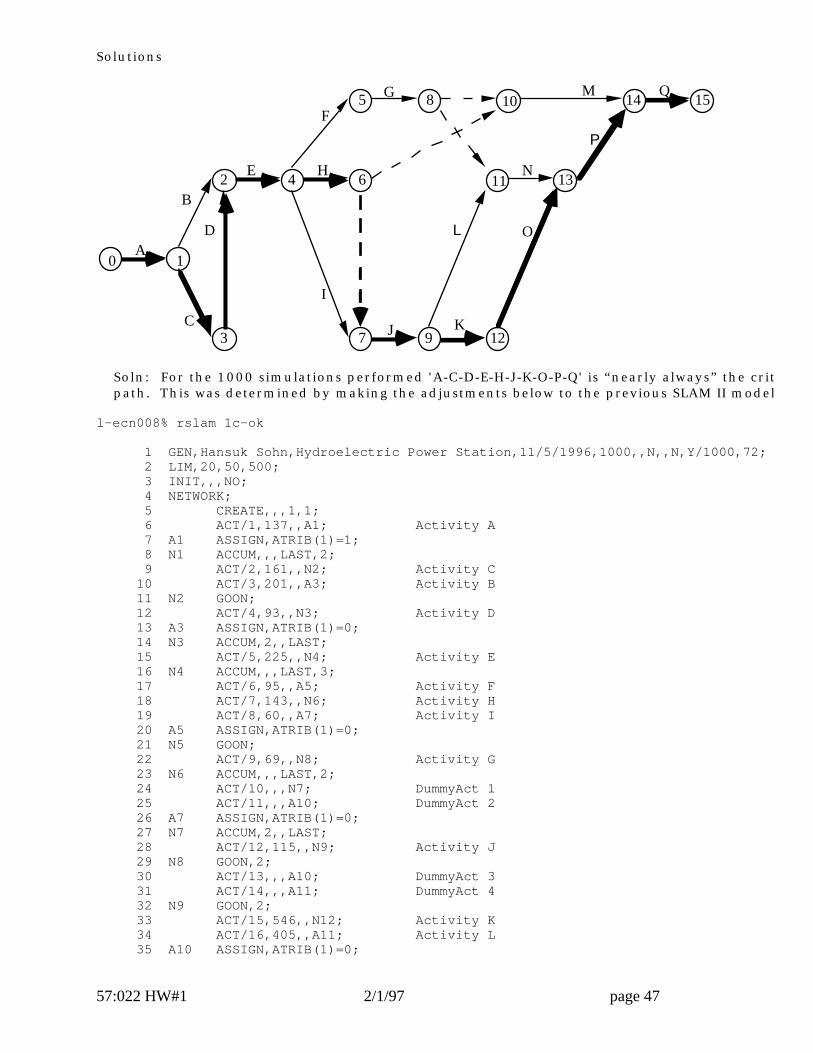
c. According to PERT, the critical path which you found in Homework #8, assumingthe durations to be equal to their expected values, namely

[A - C - D - E - H - J - K - O - P - Q],is always the critical path. Determine whether that is true for the 1000simulations you have performed. (Because of the relatively large “float” of thenoncritical activities found in Homework #8, it might be true. If necessary,modify your SLAM model to determine this!) If not true, in how many simulationswas this path not the critical path?

Solutions

57:022 HW#1 2/1/97 page 47

A

B

C

D

E

F

G

H

I

J K

M

N

O

Q

L

P

0 1

2

3

4

5

6

7

8

9

10

11

12

13

14 15

Soln: For the 1000 simulations performed 'A-C-D-E-H-J-K-O-P-Q' is “nearly always” the criticalpath. This was determined by making the adjustments below to the previous SLAM II model.

l-ecn008% rslam 1c-ok

1 GEN,Hansuk Sohn,Hydroelectric Power Station,11/5/1996,1000,,N,,N,Y/1000,72; 2 LIM,20,50,500; 3 INIT,,,NO; 4 NETWORK; 5 CREATE,,,1,1; 6 ACT/1,137,,A1; Activity A 7 A1 ASSIGN,ATRIB(1)=1; 8 N1 ACCUM,,,LAST,2; 9 ACT/2,161,,N2; Activity C 10 ACT/3,201,,A3; Activity B 11 N2 GOON; 12 ACT/4,93,,N3; Activity D 13 A3 ASSIGN,ATRIB(1)=0; 14 N3 ACCUM,2,,LAST; 15 ACT/5,225,,N4; Activity E 16 N4 ACCUM,,,LAST,3; 17 ACT/6,95,,A5; Activity F 18 ACT/7,143,,N6; Activity H 19 ACT/8,60,,A7; Activity I 20 A5 ASSIGN,ATRIB(1)=0; 21 N5 GOON; 22 ACT/9,69,,N8; Activity G 23 N6 ACCUM,,,LAST,2; 24 ACT/10,,,N7; DummyAct 1 25 ACT/11,,,A10; DummyAct 2 26 A7 ASSIGN,ATRIB(1)=0; 27 N7 ACCUM,2,,LAST; 28 ACT/12,115,,N9; Activity J 29 N8 GOON,2; 30 ACT/13,,,A10; DummyAct 3 31 ACT/14,,,A11; DummyAct 4 32 N9 GOON,2; 33 ACT/15,546,,N12; Activity K 34 ACT/16,405,,A11; Activity L 35 A10 ASSIGN,ATRIB(1)=0;

Solutions

57:022 HW#1 2/1/97 page 48

36 N10 ACCUM,2,,LAST; 37 ACT/17,447,,N14; Activity M 38 A11 ASSIGN,ATRIB(1)=0; 39 N11 ACCUM,2,,LAST; 40 ACT/18,150,,N13; Activity N 41 N12 GOON; 42 ACT/19,47,,N13; Activity O 43 N13 ACCUM,2,,LAST; 44 ACT/20,27,,N14; Activity P 45 N14 ACCUM,2,,LAST; 46 ACT/21,25,,CHECK; Activity Q 47 CHECK COLCT,ATRIB(1),Number_Same_CP 48 EFT COLCT,FIRST,Earliest_Finish_Time 49 TERM,1; 50 END; 51 FIN;


SIMULATION PROJECT HYDROELECTRIC POWER BY HANSUK SOHN

DATE 11/ 5/1996 RUN NUMBER 1000 OF 1000




NUMBER_SAME_CP 100E+01 .000E+00 .000E+00 .100E+01 .100E+01 1000 EARLIEST_FINISH_ .152E+04 .000E+00 .000E+00 .152E+04 .152E+04 1000

A new COLCT node was inserted to collect statistics on the value of ATTRIBUTE #1,which is equal to 1 if the path of interest [A - C - D - E - H - J - K - O - P - Q] iscritical, and zero otherwise. We see that the minimum value and maximum value ofattribute #1 are both equal to 1, indicating that the path was always the longestpath in the network. Warning: this isn’t true in general! In this particularexample, all noncritical activities had rather large values of slack (“float”), asfound in the previous homework assignment!

Based upon your simulation, if you wish to set a deadline for completion of the projectso that you are 90% certain of meeting this deadline, what should this deadline be?

Sol’n: See the histogram of the project completion time. 36 .036 .1549+04 +** C + 29 .029 .1552+04 +* C +

By summing the counts of the cells, we find that at time=1549 days, 875 (i.e., 87.5%) ofthe simulated projects had been completed, while at time=1552 days, 904 (i.e. 90.4%) ofthe projects had been completed. Using a linear interpolation, we estimate that 90% ofthe simulated projects should be completed at time= 1549+ 3(25/29) = 1551.6 days.

To get a more accurate estimate of the correct warranty period, we should• increase the number of runs from 1000, e.g., to as many as 10000

Solutions

57:022 HW#1 2/1/97 page 49

• change the specifications for the histogram so as to get a count of failures eachday, e.g.,

EFT COLCT,FIRST,Earliest_Finish_Time,50/1545/0.05which would give 50 cells, each of length 0.05 days.

e. Suppose that, by using improved procedures, the variability in the duration ofactivity J, “Arrange construction mat’ls supply”, which presently is ± 15 days, might

be reduced to ± 5 days. How would this effect the deadline which you set in (d)?

Sol’n: Modify the SLAM statement for activity J, i.e.,

24 ACT/12,TRIAG( 110, 115 ,120 ),,N9; Activity J +/- 5

and re-run the simulation. In the new histogram, we find that at time=1548 days 895projects had been completed, and at time=1551, 918 projects had been completed:

38 .038 .1548+04 +** C + 23 .023 .1551+04 +* C +

Using linear interpolation as before, we estimate that 900 projects would be complete attime = 1548 + 3(5/23) = 1548.7 days (2.9 days earlier than estimated in part (d).)

To get a more accurate estimate of the correct warranty period, we should• increase the number of runs from 1000, e.g., to as many as 10000• change the specifications for the histogram so as to get a count of failures each

day, e.g.,EFT COLCT,FIRST,Earliest_Finish_Time,50/1543/0.1

which would give 50 cells, each of length 0.1 days.

f. According to PERT, the project duration should have approximately a normaldistribution. Use the chi-square goodness of fit test to determine whether thisassumption is valid for this project.

Solution: To reduce the computational burden somewhat, the below table wascomputed with each interval of 6 days length, rather than the 3 days in the SLAMhistogram. Using normal distribution tables with mean µ = 1520 and standard

deviation σ = 19, we compute the probability pi that one of the 1000 observationsfalls into cell #i, and then multiply this by 1000 to get Ei , the expected number ofobservations in cell #i:

# Interval Oi Ei Pi Oi - Ei2

Ei1 1470 - 1475 2 4.682 0.004682 1.536335752 1475 - 1480 3 8.648 0.008648 3.688703053 1480 - 1485 3 14.980 0.014980 9.580801074 1485 - 1490 12 24.354 0.024354 6.266786405 1490 - 1495 25 37.068 0.037068 3.928904286 1495 - 1500 55 52.590 0.052590 0.110441157 1500 - 1505 59 69.306 0.069306 1.532531618 1505 - 1510 68 84.775 0.084775 3.319382199 1510 - 1515 92 96.525 0.096525 0.21212769

10 1515 - 1520 84 102.802 0.102802 3.43879695

Solutions

57:022 HW#1 2/1/97 page 50

11 1520 - 1525 99 102.802 0.102802 0.1406120912 1525 - 1530 112 96.525 0.096525 2.4809699613 1530 - 1535 66 84.775 0.084775 4.1580728414 1535 - 1540 85 69.306 0.069306 3.5538284715 1540 - 1545 74 52.590 0.052590 8.7162597516 1545 - 1550 53 37.068 0.037068 6.8476482117 1550 - 1555 50 24.354 0.024354 27.0065417018 1555 - 1560 25 14.980 0.014980 6.7022964019 1560 - 1565 17 8.648 0.008648 8.0661313620 1565 - 1570 9 4.682 0.004682 3.9822990221 1570 - 1575 3 2.368 0.002368 0.1686756822 1575 - 1580 4 1.110 0.001110 7.52441441

sum = 1000 D = 112.96256000

Note : pi = F(ti ) − F(ti−1 ) ∀ i ≥1 , where t~ N(1520,19) Thus, for example,

∴ p1 = F(t1 ) − F(t0) = F(1475) - F(1470) = 0.004682

∴ E1 = 1000× P1 = 4.682

p1 = F(t1 ) − F(t0) = F(1480) - F(1475) = 0.008648

∴ E2 = 1000× P2 = 8.648

We perform a Chi-Square Goodness of Fit test to determine whether this normaldistribution provides an acceptable fit to the observed data, with α = 5%.

Since " D ( 112.96) > χ5%2 (= 30.15) ", we can conclude that this distribution does not

provide an acceptable fit to the observed data with α =5%.

•••••••••••••••••••••••••••• Homework # 10 ••••••••••••••••••••••••••••••••1. Consider an inventory system in which the number of items on the shelf ischecked at the end of each day. The maximum number on the shelf is 8. If 3 orfewer units are on the shelf, the shelf is refilled overnight. The demanddistribution is as follows:

x 0 1 2 3 4 5 6P{D=x} .1 .15 .25 .25 .15 .05 .05

The system is modeled as a Markov chain, with the state defined as the number ofunits on the shelf at the end of each day. The probability transition matrix is:

Solutions

57:022 HW#1 2/1/97 page 51

a. Explain the derivation of the values P19, P35, P51, P83 above. (Note thatstate 1=inventory level 0, etc.)

State Definition

1 SOH = 0 2 SOH = 1 3 SOH = 2 4 SOH = 3 5 SOH = 4 6 SOH = 5 7 SOH = 6 8 SOH = 7 9 SOH = 8

Solution: P ij = P Xn = j|Xn−1 = i{ }if i > 4 (SOH >3), no replenishment occurs :

P ij =P D = (i − j){ }P D ≥ (i − j){ }

for j >1 (SOH > 0)

for j =1 (SOH = 0)

∴ P 83 = P D = (8-3) =5{ } = 0.05P 51 = P D ≥ (5-1)= 4{ }= 0.15 + 0.05 + 0.05 = 0.25

if i ≤ 5 (SOH ≤ 4), the SOH at the beginning of the next day is 8 :P ij = P D = 8-(j-1)( ){ }

∴ P19 = P D = 8-(9-1)( ){ } = P D = 0{ } = 0.1

P 35 = P D = 8-(5-1)( ){ } = P D = 4{ } = 0.15

The steady-state distribution of the above Markov chain is:

Solutions

57:022 HW#1 2/1/97 page 52

b. Write two of the equations which define this steady-state distribution. Howmany equations must be solved to yield the solution above?

Solution: 9 equations must be solved to compute the values of the 9probabilities. One equation must be

π1 + π2 + π3 + π4 + π5 + π6 + π7 + π8 + π9 =1while the remaining 8 are obtained by setting πi equal to the inner product of

column i and π. For example, using column i=1 we would obtain the equation

π1 = 0.25π5 + 0.1π6 + 0.05π7

c. What is the average number on the shelf at the end of each day?

Solution: Since in state i the stock on hand is (i-1),

Average Stock-on-Hand = i − 1( )i =1

9

∑ πi = 4.968123

The mean first passage matrix is:

d. If the shelf is full Monday morning, what is the expected number of daysuntil the shelf is first emptied ("stockout")?

Solution: m91 = 15.4523 (days)e. What is the expected time between stockouts? Solution: m00 = 15.4523 (days)f. How frequently will the shelf be restocked? (i.e. what is the average

number of days between restocking?)

Solutions

57:022 HW#1 2/1/97 page 53

Solution: Since the shelf is restocked whenever the state of the system is1,2,3, or 4, the steadystate probability that the shelf is restocked on a day is

i=1

4

∑ π = 0.4076 = 1/2.4534,

i.e., we expect the shelf to restocked with frequency once each 2.4534 days.

2. Consider a manufacturing process in which raw parts (blanks) are machined onthree machines, and inspected after each machining operation. The relevant datais as follows:

For example, machine #1 requires 0.5 hrs, at $20/hr., and has a 10% scrap rate. Thoseparts completing this operation are inspected, requiring 0.1 hr. at $15/hr. Theinspector scraps 10%, and sends 5% back to machine #1 for rework (after which itis again inspected, etc.)

The Markov chain model of a part moving through this system has transitionprobability matrix:

a. Draw the diagram for this Markov chain and describe each state.Solution:

Solutions

57:022 HW#1 2/1/97 page 54

1 2 3 4 5 6 7

8

0.05 0.03 0.02

0.1 0.1 0.05 0.1 0.02 0.05

1

1

0.9 0.85 0.95 0.87 0.98 0.93

State Location

1 Machine1 2 Inspection station1 3 Machine2 4 Inspection station2 5 Machine3 6 Inspection station3 7 Pack-&-Ship Dept. 8 Scrap bin

b. Which states are transient? which are absorbing?Solution: Transient States : 1, 2, 3, 4, 5, and 6

Absorbing States : 7 and 8

The absorption probabilities are:

The matrix E is as follows:

c. Explain how matrix E was computed. Explain how matrix A was computed,given E.

Solution:

0 0.9 0 0 0 0 0 0.10.05 0 0.85 0 0 0 0 0.10 0 0 0.95 0 0 0 0.050 0 0.03 0 0.87 0 0 0.10 0 0 0 0 0.98 0 0.020 0 0 0 0.02 0 0.93 0.050 0 0 0 0 0 1 00 0 0 0 0 0 0 1

Q R

0 I=

matrices E and A could be computed by equations E = I − Q( )−1 and A=E× R,

respectively.

Solutions

57:022 HW#1 2/1/97 page 55

d. What percent of the parts which are started are successfully completed?Solution: A1,OK = 0.6335 = 63.35 %e. What is the expected number of blanks which should be required to fill an

order for 100 completed parts?

Solution: 100

A1,OK

= 100

0.6335 = 157.8532

f. What percent of the parts arriving at machine #2 will be successfullycompleted?

Solution: A 3,OK = 0.7909 = 79.09 %g. What is the expected total number of inspections which entering parts will

undergo?Solution: E12 + E14 + E16 = 2.4069h. Explain the meaning of the number appearing in row 3, column 2 of the A

matrix.Solution: A 32 = .2091 indicates that parts arriving at machine 2 have a

20.91 % probability of being failed.i. Explain the meaning of the number appearing in row 3, column 3 of the E

matrix.Solution: E33 =1.029 indicates the expected number of times that parts

arriving at machine 2 returns to machine 2 before successfully finished orfailed.

j. To fill the order for 100 completed parts, what is the expected man-hourrequirement for each machine? for each inspection station?

Solution:Operation state Man-hour / 100 completed part

Machine 1 1 1.047 0.5 (1/0.6335) 100 = 82.64 Inspection 1 2 1.047 0.1 (1/0.7039) 100 = 14.87Machine 2 3 1.029 0.75 (1/0.7909) 100 = 97.58Inspection 2 4 1.029 0.2 (1/0.8325) 100 = 24.72Machine 3 5 1.02 0.25 (1/0.9296) 100 = 27.43Inspection 3 6 1.02 0.25 (1/0.9486) 100 = 26.88Pack-&-Ship 7 1 0.1 (1/1) 100 = 10

Total = 284.12

× × ×× × ×× × ×× × ×× × ×× × ×× × ×

k. What are the expected direct costs (row materials + operating costs - scrapvalue of rejected parts) per completed part?

Solution:Each completed part requires an expected 1/0.6335, i.e., 1.5785 enteringparts.Materials : $ 50 × 1.5785 = $ 78.925Scrap value of rejected parts : $ 10 × 1.5785 × 0.3665 = $ 5.785Estimated Man-hour requirements per completed part

Solutions

57:022 HW#1 2/1/97 page 56

Operation state Man-hour / completed part

Machine 1 1 1.047 0.5 (1/0.6335) = 0.8264 Inspection 1 2 1.047 0.1 (1/0.7039) = 0.1487Machine 2 3 1.029 0.75 (1/0.7909) = 0.9758Inspection 2 4 1.029 0.2 (1/0.8325) = 0.2472Machine 3 5 1.02 0.25 (1/0.9296) = 0.2743Inspection 3 6 1.02 0.25 (1/0.9486) = 0.2688Pack-&-Ship 7 1 0.1 (1/1) = 0.1

Total = 2.8412

× ×× ×× ×× ×× ×× ×× ×

Operation cost :

Operation state Hourly Rate Man-Hours

Machine 1 1 20 0.8264 = 16.528 Inspection 1 2 15 0.1487 = 2.2305Machine 2 3 20 0.9758 = 19.516Inspection 2 4 15 0.2472 = 3.708Machine 3 5 20 0.2743 = 5.486Inspection 3 6 15 0.2688 = 4.032Pack-&-Ship 7 10 0.1 = 1

Total = $ 52.5005

×

×××××××

Total Direct Cost = row material + operating costs - Scrap value of rejectedparts

= $ 78.925 + $ 52.5005 - $ 5.785 = 125.6405

3. A city's water supply comes from a reservoir. Careful study of this reservoir overthe past 20 years has shown that, if the reservoir was full at the beginning of thesummer, then the probability it would be full at the beginning of the followingsummer is 80%. On the other hand, if the reservoir was not full at the beginning ofone summer, the probability it would be full at the beginning of the followingsummer is only 25%.

a. Defining the states to be "full" and "not full", draw a transition diagram for aMarkov chain model of this reservoir.

Solution:

state definition

1 full 2 not full

0.800.20

0.25

0.75

1 2

b. Write the transition probability matrix.

Solution:

P =0.80 0.20

0.25 0.75

Solutions

57:022 HW#1 2/1/97 page 57

c. If the reservoir was full at the beginning of summer 1996, what is theprobability that it will be full at the beginning of summer 1998?

Solution: P112 = 0.69

from P2 =

0.6900 0.3100

0.3875 0.6125

d. Write equations which determine the steadystate probability distribution forthis Markov chain, and solve them.

Solution:π1 = 0.80π1 + 0.25π 2

π1 + π 2 = 1

or π2 = 0.20π1 + 0.75π2

π1 + π 2 = 1

∴π1 =5

9 , π 2 =

4

9e. Over a long period of time, in what percent of the years would we expect the

reservoir be full at the beginning of the summer, according to this model?

Solution: π1 =5

9 = 55.56 %

homework solutions fall 1996 - user page server for...

Documents