Transpn Rer-E Vol. 16B. No. 6. pp. 459470. 1982 0191-?615/82/060459-1?503.0010

Printed in Great Britain 0 1982 Pergamon Press Ltd.

HOMOGENEOUS OPTIMAL FLEET

I. GERTSBAKH and YURI GUREVICH

Ben Gurion University of the Negev, Beersheva, Israel

(Received 22 January 1981; in revised form 15 December 1981)

Abstract-The structure of chains in the optimal chain decomposition of a periodic schedule S is investigated. A finite oriented graph termed the Linis Graph (LG) is defined which serves as the key for this investigation. The edges of the LG are trip-types of S and the vertices of the LG represent terminals. It is proved that there is an Euler cycle for a connected LG satisfying natural precedence relations between arrival and departure times. Expansion of this cycle in a real time gives a “master-chain” of trips which, being repeated periodically, gives an infinite periodic chain. Time-shifted periodic replication of this chain allows obtaining a group of twin-type periodic chains forming an optimal fleet over S. It is proved that if the LG has m connected components then there is an optimal fleet consisting of m groups of similar periodic chains. It is shown that if the graph of terminals is connected and the LG is disconnected then it is possible to obtain a twin-type fleet over S by adding to S “dummy” trip-types. A general approach to constructing a twin-type fleet of minimal size for this case is described. The relation of the theory developed to the so-called center problem is discussed.

1. INTRODUCTION

This paper treats some problems arising in the latest stages of planning transportation activities. Assume that the following decisions have been already made: trips which have to be carried out during the planning period (say, a year) are chosen; a preliminary estimation of the fleet size has been made and possible changes in the departure/arrival times in order to minimize the fleet size have been already done. (It is assumed that each vehicle can carry out any trip in the schedule.) The next phase in planning transportation work should be constructing routes for individual vehicles, or more formally, decomposing the schedule into chains each of which represent a sequence of trips carried out by one physical vehicle. If this decomposition is made properly, the minimal fleet size should be equal to a certain constant determined in the following way (see Bartlett (1957), Salzborn (1974), Linis and Maksim (1967), Gertsbakh and Gurevich (1977)): let d,(t) be an integer valued function defined as the difference between the number of departures and arrivals occuring at terminal a during the time [0, t]. Then the minimal fleet size (MFS) is equal to the total deficit, D:

(Here the sum is taken over the set A of all terminals appearing in the schedule.) The chains in the optimal decomposition constitute an important object for solving further

problems connected with the implementation of the schedule, namely, the assignment of crews to trips and vehicles and the maintenance of the vehicles. The structure of chains in the optimal chain decomposition will be the main subject of this paper.

In this paper we deal with purely periodic schedules. This means that there is a time unit called the period (a week, a day, etc.) such that all trips whose departures take place in a period are always repeated in the next one.

Periodic schedules are widely used in different kinds of transportation systems because they attract more passengers: people prefer to use stable, periodically repeated trips to which they get accustomed to in the course of time. In addition, the periodic component of the schedule usually serves as a frame for the whole time-table to which additional trips should be added according to passenger demand during the peak periods.

In this paper we shall investigate the possibility of decomposing the schedule into a number of periodic twin-type chains. Such decomposition makes every vehicle to repeat the same sequence of trips where each sequence contains “twins” of all trips appearing in one period. This implies that the arrival times of any vehicle to any given terminal contain a periodic subsequence of times to, to+ T*, to+ 2T*, . . . , to+ /CT*, . . . , period T* being the same for all vehicles. Thus each vehicle does the same amount of transportation work during time T* (say,

459

460 I. GERTSBAKH an;l YURI GuREVICH

the same total mileage) and visits all terminals mentioned in the schedule. Therefore, all vehicles are in similar conditions and the total transportation work is uniformly distributed between them. It is a common rule to send each vehicle to maintenance after completing a fixed amount of work (e.g. an aircraft has to be checked after each 500 hr spent in the air). A twin-type fleet allows to distribute the maintenance times uniformly over any calendar period for each vehicle thus providing a uniform load distribution for repair facilities. Besides, if these facilities are located in a terminal mentioned in the schedule no additional trips will be needed to provide arrival of vehicles to the repair station.

Twin-type fleet might be convenient for crew scheduling because an assignment of one or several crews to each vehicle provides automatically that all crews will have the same load. Also the process of computerized scheduling simplifies considerably when the chains are of twin-type. It is worth noting that practical scheduling experts prefer usually to think about the schedule in terms of chains; here again twin-type representation is convenient for manual and graphical operation.

Let us term the fleet which consists of groups of similar periodic chains as homogeneous. The main subject of this paper is to develop a theory for constructing a homogeneous optimal fleet.

Let us consider an example illustrating our results and providing an intuitive background for their derivation.

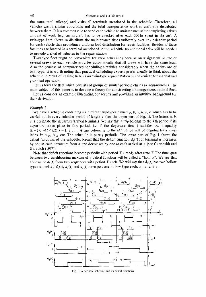
Example 1 We have a schedule containing six different trip-types named a, p, y, 6, cp, $ which has to be

carried out in every calendar period of length T (see the upper part of Fig. 1). The letters a, b, c, e designate the departure/arrival terminals. We say that a trip belongs to the kth period if its departure takes place in this period, i.e. if the departure time t satisfies the inequality (k - l)T s t < kT, k = 1, 2,. . . . A trip belonging to the kth period will be denoted by a lower

index k: a(k), P(k), etc. The schedule is purely periodic. The lower part of Fig. 1 shows the deficit functions of the schedule. Recall that the deficit function d,(t) for terminal a increases by one at each departure from a and decreases by one at each arrival at a (see Gertsbakh and

Gurevich (1977)). Note that deficit functions become periodic with period T already after time T. The time span

between two neighbouring maxima of a deficit function will be called a “hollow”. We see that hollows of d,,(t) form two sequences with period T each. We will say that dh(t) has two hollow types b, and b,. d,(t), d,(t) and d,(t) have just one hollow type each: a,, c, and e,.

d,(t )

2

I

dbW) I

d&t )

I

d,(t) I

Fig. I. A periodic schedule and its deficit functions.

Homogeneous optimal fleet 461

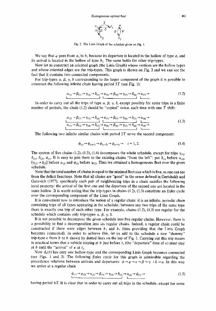
Fig. 2. The Linis Graph of the schedule given on Fig. 1.

We say that cp goes from a, to b, because its departure is located in the hollow of type a, and its arrival is located in the hollow of type b,. The same holds for other trip-types.

Now let us construct an oriented graph (the Linis Graph) whose vertices are the hollow types and whose oriented edges are the trip-types. This graph is shown on Fig. 2 and we can see the fact that it contains two connected components.

For trip-types (Y, p, y, S corresponding to the larger component of the graph it is possible to construct the following infinite chain having period 3T (see Fig. 1):

?I)+ Pm+ Y(Z)-+ so,+ q4)‘P(4)’ Y(s)+ a(6)’ (Y(7)’ (1.2)

MI__

In order to carry out all the trips of type (Y, p, y, 6, except possibly for some trips in a finite number of periods, the chain (1.2) should be “copied” twice, each time with one T shift:

a(2) + P(2) + Y(3) + a(4) + a,S) + P(S) += Y(6) -+ s(7) + a,S) +

LII (1.3) a(3) + P(3) + Y(4) + &5) + a(6) + P(6) + Y(7) -+ &.) + a(9) +

II-

The following two infinite similar chains with period 2T serve the second component:

The system of five chains (1.2), (1.3), (1.4) decomposes the whole schedule, except for trips y(,,, S,,,, Sc2), I/+,,. It is easy to join them to the existing chains “from the left”: put S,,, before (Yak),

{y(,)+ S,2,} before (Y,~) and &,, before (pc2). Thus we obtained a homogeneous fleet over the given schedule.

Note that the total number of chains is equal to the minimal fleet size which is five, as one can see from the deficit functions. Note that all chains are “good” in the sense defined in Gertsbakh and Gurevich (1977), specifically each pair of neighbouring trips in a chain satisfies the following local property: the arrival of the first one and the departure of the second one are located in the same hollow. It is worth noting that the trip-types in chains (1.2), (1.3) constitute an Euler cycle over the corresponding component of the Linis Graph.

It is convenient now to introduce the notion of a regular chain: it is an infinite, periodic chain containing trips of all types appearing in the schedule; between any two trips of the same type there is exactly one trip of each other type. For example, chains (1.2), (1.3) are regular for the schedule which contains only trip-types (Y, p, y, 6.

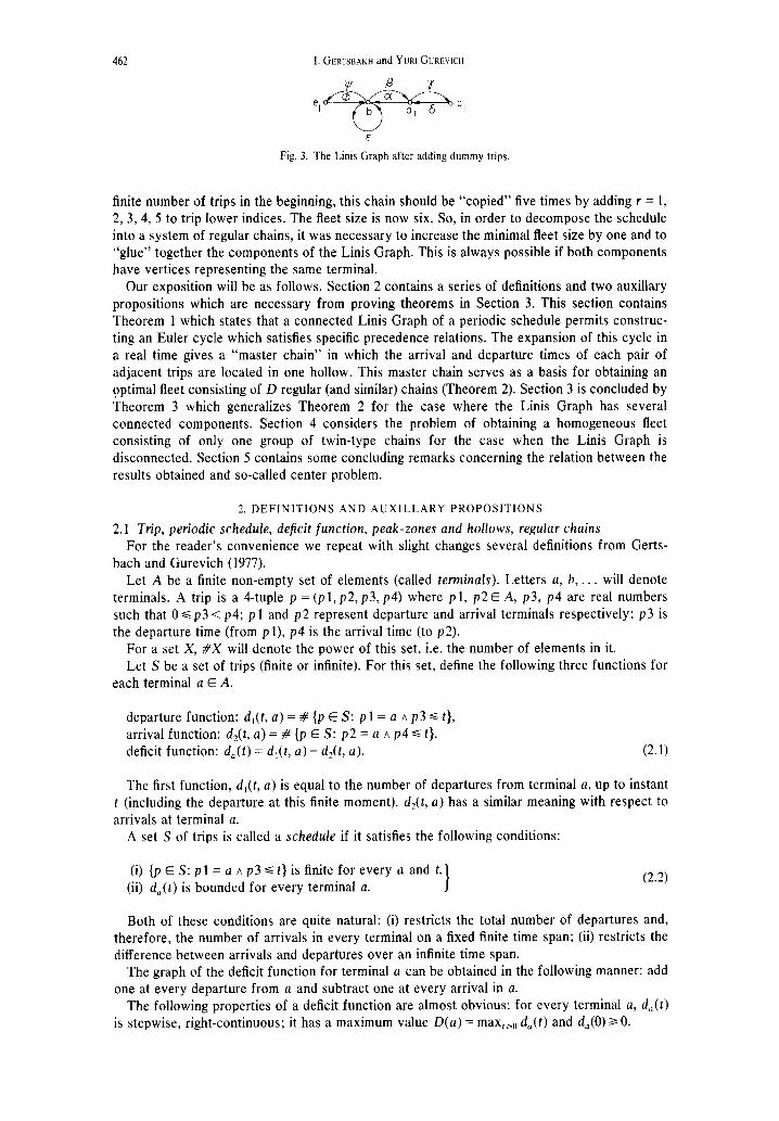
It is not possible to decompose the given schedule into five regular chains. However, there is a possibility to find a decomposition into six regular chains. Indeed, a regular chain could be constructed if there were edges between b, and b, (thus providing that the Linis Graph becomes connected). In order to achieve this, let us add to the schedule a new “dummy” trip-type E from b to b shown by dotted lines on the top of Fig. 1. Carrying out this trip means in practical terms that a vehicle staying at b just before t, (the “departure” time of E) must stay at b until the “arrival” of E at t,.

Now r&(t) has only one hollow-type and the corresponding Linis Graph becomes connected (see Figs. 1 and 3). The following Euler cycle for this graph is admissible regarding the precedence relations between arrivals and departures: I,!J + cp + E + /3 + y + S + (Y. In this way we arrive at a regular chain

h) -+ (P(2) + E(3) + P(3) + Y(4) -+ &5) -+ a,6) + Icr(7) + (1.5) 1 I I

having period 6T. It is clear that in order to carry out all trips in the schedule, except for some

462 LGERTSBAKH and Y URI GUREVICH

Fig. 3. The Link Graph after adding dummy trips.

finite number of trips in the beginning, this chain should be “copied” five times by adding r = 1, 2, 3,4, 5 to trip lower indices. The fleet size is now six. So, in order to decompose the schedule into a system of regular chains, it was necessary to increase the minimal fleet size by one and to “glue” together the components of the Linis Graph. This is always possible if both components have vertices representing the same terminal.

Our exposition will be as follows. Section 2 contains a series of definitions and two auxillary propositions which are necessary from proving theorems in Section 3. This section contains Theorem 1 which states that a connected Linis Graph of a periodic schedule permits construc- ting an Euler cycle which satisfies specific precedence relations. The expansion of this cycle in a real time gives a “master chain” in which the arrival and departure times of each pair of adjacent trips are located in one hollow. This master chain serves as a basis for obtaining an optimal fleet consisting of D regular (and similar) chains (Theorem 2). Section 3 is concluded by Theorem 3 which generalizes Theorem 2 for the case where the Linis Graph has several connected components. Section 4 considers the problem of obtaining a homogeneous fleet consisting of only one group of twin-type chains for the case when the Linis Graph is disconnected. Section 5 contains some concluding remarks concerning the relation between the results obtained and so-called center problem.

2. DEFINITIONS AND AUXILLARY PROPOSITIONS

2.1 Trip, periodic schedule, deficit function, peak-zones and hollows, regular chains For the reader’s convenience we repeat with slight changes several definitions from Gerts-

bath and Gurevich (1977). Let A be a finite non-empty set of elements (called terminals). Letters a, b, . . . will denote

terminals. A trip is a 4-tuple p = (p 1, p2, p3, p4) where p 1, p2 E A, p3, p4 are real numbers such that 06~3 < p4; pl and p2 represent departure and arrival terminals respectively; p3 is the departure time (from p l), p4 is the arrival time (to ~2).

For a set X, #X will denote the power of this set, i.e. the number of elements in it. Let S be a set of trips (finite or infinite). For this set, define the following three functions for

each terminal a E A.

departure function: d,(t, a) = # {p E S: p 1 = a A p3 s t}, arrival function: d2(t, a) = # {p E S: p2 = a A p4 < t}. deficit function: d,(t) = d,(t, a) - d,(t, a). (2.1)

The first function, d,(t, a) is equal to the number of departures from terminal a, up to instant t (including the departure at this finite moment). d,(t, a) has a similar meaning with respect to arrivals at terminal a.

A set S of trips is called a schedule if it satisfies the following conditions:

(i) {pES:pl=ar,p3st}isfiniteforeveryaand t. (ii) d,(t) is bounded for every terminal a. I

(2.2)

Both of these conditions are quite natural: (i) restricts the total number of departures and, therefore, the number of arrivals in every terminal on a fixed finite time span; (ii) restricts the difference between arrivals and departures over an infinite time span.

The graph of the deficit function for terminal a can be obtained in the following manner: add one at every departure from a and subtract one at every arrival in a.

The following properties of a deficit function are almost obvious: for every terminal a, d,(t) is stepwise, right-continuous; it has a maximum value D(a) = max,,” d,(t) and d,(O) 2 0.

Homogeneous optimal fleet 463

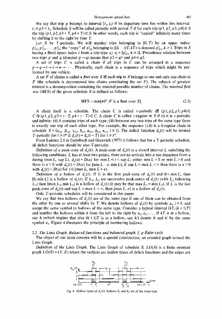
We say that trip p belongs to interval [t,, t2) if its departure time lies within this interval: t, < p3 < t,. Schedule S will be called periodic with period T if for each trip (p 1, p2, p3, ~4) E S the trip (p 1, ~2, p3 + T, p4 + T) E S. In other words, each trip is “copied” infinitely many times by shifting it to the right by time T.

Let S be T-periodic. We will number trips belonging to [0, T) by an upper index:

PI,,, P:,,, . . . , P;,,; the “COPY” Of P{,, belonging to [(k - l)T, kT) is denoted p&), k 2 1. Trips in S having a fixed upper index i form a trip-type ei: ei = {pfk), k 2 1). Precedence relation between two trips p and q (denoted p + q) means that p2 = q 1 and p4 s q3.

A set of trips C is called a chain if all trips in C can be arranged in a sequence p-+qdr+s+W+‘. . . Physically, each chain is a sequence of trips which might be per- formed by one vehicle.

A set F of chains is called a fleet over S iff each trip in S belongs to one and only one chain in F (the schedule is decomposed into chains constituting the set F). The subject of greatest interest is a decomposition containing the minimal possible number of chains. The minimal fleet size (MFS) of the given schedule S is defined as follows:

MFS = min{#F: F is a fleet over S}. (2.3)

A chain itself is a schedule. The chain C is called T-periodic iff (~1, ~2, ~3, ~4) E C + (p 1, ~2, p3 + T + T, p4 + T . T) E C. A chain C is called T-regular in S if (i) it is qXXiOdiC

and infinite; (ii) it contains trips of each type; (iii) between any two. trips of the same type there is exactly one trip of each other type. For example, the sequence (1.6) is a 6-regular chain in

schedule S = {a(i), P(i), y(i), S,i,, p(i), +ci,, E(i), i 3 1). The deficit function d,(t) will be termed T-periodic for t 2 t* if d,(t) = d,(t + T) for t 3 t*.

From Lemma 2.1 in Gertsbach and Gurevich (1977) it follows that for a T-periodic schedule, all deficit functions should be also T-periodic.

Definition of a peak-zone of d,(t). A peak-zone of d,(t) is a closed interval L satisfying the following conditions: L has at least two points, there are no arrivals into a nor departure from a during (min L, sup L), d,(t) = D(a) for min L <t<supL; either minL=O or minL>O and there is E > 0 with d,(t) < D(a) for [min L - E, min L); if sup L = max L <m then there is E > 0 with d,(t) < D(a) for t E [max L, max L + l ).

Definition of a hollow of d,(t). If L is the first peak-zone of d,(t) and 0 <min L, then [0, min L] is a hollow of d,(t). If L,, L, are successive peak-zones of d,(t) (with L, following L,) then [max L,, min L2] is a hollow of d,(t) (it may be that max L, = min L,). If L is the last peak-zone of d,(t) and sup L = max L < cc, then [max L, m) is a hollow of d,(t).

Only T-periodic schedules will be considered in this paper. We say that two hollows of d,(t) are of the same type if one of them can be obtained from

the other by one or several shifts by T. We denote hollows of d,(t) by symbols ai, i 2 1, and assign the same symbol to hollows of the same type. Consider a typical interval [kT, (k + l)T] and number the hollows within it from the left to the right by a,, a2,. . . . If kT is in a hollow, say h (which implies that also (k + l)T is in a hollow, say h’) denote h and h’ by the same symbol a,. Figure 4 illustrates the principle of numbering hollows.

2.2 The Linis Graph. Balanced functions and balanced graph. f, g-Euler cycle The object of our main concern will be a special construction, an oriented graph termed the

Linis Graph. Dejinition of the Linis Graph. The Linis Graph of schedule S, LG(S) is a finite oriented

graph LG(S) = (V, E) where the vertices are hollow types of deficit functions and the edges are

d, (t)

3

2

I ime

(K-I)T t; t’; kT I II

t2 ‘2 (KiI)T t

Fig. 4. Hollow types of d,(r): hollows h, and hz are of the same type.

464 I. GERTSBAKH and YLW GUREVICH

trip-types; if trip e = (el, e2, e3, e4) E S is of type ei E E, e3 is located in a hollow of type el,, e4 is located in a hollow of type e2i, then edge e, comes out from vertex el, and enters vertex e2i. (See Introduction for examples of LG(S)).

A nonformal description of the Linis Graph is given in the paper of Linis and Maksim (1967), Section 4.

In LG(S) each vertex v E V has even degree: the number of edges entering v is equal to the number of edges coming out from v.

Assume that LG(S) is connected. We want to construct a Euler cycle (i.e. a closed tour containing all edges, each only once) satisfying the following condition: if e, e’ are successive edges in the cycle and p, p’ are trips of trip-types e, e’, respectively, p4 and p’3 are located in the same hollow, then

p4sp’3. (2.4)

Specific relationship between arrival-departure times of trips which are located in one hollow motivate the following:

Definition of balanced functions. Let Z, J be finite sets, R be the set of reals and f : I + R, g : J -+ R (i.e. f, g are finite real-valued functions with domains Z, J, respectively). f and g are balanced if either Z and J are empty or (i) #Z = #J and (ii) Id,,(t) = # {j: g(j)< t, j EJ}- # {i: f(i) s t, i E I} is negative in the interval [min mgf, max mgg) and zero outside it. Id,(t) will be termed the local deficit function of f, g. In the case when Z and J are edges entering vertex v and coming from v, respectively, (i) means that the number of edges entering v is equal to the number of edges leaving v. The values of f, f(l), . . . ,f(k), represent arrival times at v and the values of g, g(l), g(2), . . . , g(k) represent departure times from v. (ii) is a precise description that these times are located in one hollow: in any point between the earliest arrival and the latest departure the local deficit function is negative.

Note that if f and g are balanced, then min mgf < min mgg and max mgf < max mgg. Instead of “Id,,(t) is zero outside [min mgf, max mgg)” it suffices to request “the local deficit function is nonpositive everywhere”. .

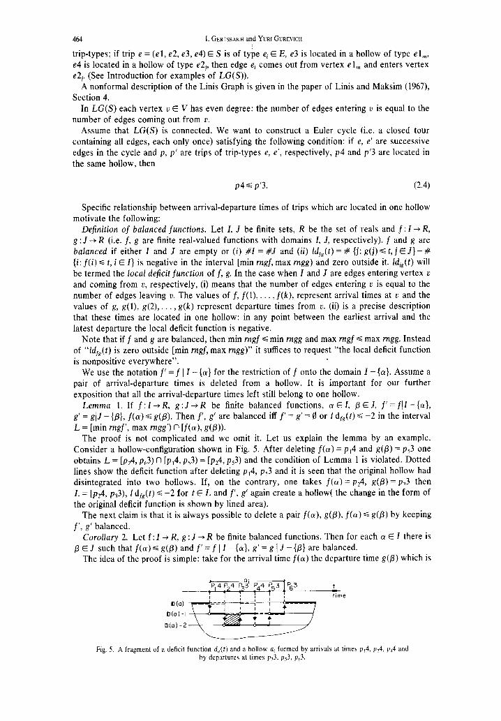
We use the notation f’ = f 1 Z -{a} for the restriction of f onto the domain Z - {cx}. Assume a pair of arrival-departure times is deleted from a hollow. It is important for our further exposition that all the arrival-departure times left still belong to one hollow.

Lemma 1. If f : Z +R, g : J + R be finite balanced functions, (Y E I, /3 E J, f’ = f\Z -{a}, g’ = g/J - {p}, f(a) < g(p). Then f’, g’ are balanced iff f’ = g’ = 0 or I d,(t) < -2 in the interval

L = [min rngf’, max mgg’) n [f(a), g(p)). The proof is not complicated and we omit it. Let us explain the lemma by an example.

Consider a hollow-configuration shown in Fig. 5. After deleting f(a) = p,4 and g(p) = p,3 one obtains L = [p24, ~~3) fl [p,4, ps3) = [p24, p53) and the condition of Lemma 1 is violated. Dotted lines show the deficit function after deleting p,4, p,3 and it is seen that the original hollow had disintegrated into two hollows. If, on the contrary, one takes f(a) = p24, g(p) = pi3 then

L = [p24, p33), I d,(t). < -2 for t E L and f’, g’ again create a hollow( the change in the form of the original deficit function is shown by lined area).

The next claim is that it is always possible to delete a pair f(a), g(p), f(a) s g(p) by keeping f’, g’ balanced.

Corollary 2. Let f: Z + R, g : J -+ R be finite balanced functions. Then for each a! E Z there is p E J such that f(a) < g(p) and f’ = f ( Z -{a}, g' = g 1 J -{p} are balanced.

The idea of the proof is simple: take for the arrival time f(a) the departure time g(p) which is

jzqTP3p33i P44 PS 3 P63 t

time

Fig. 5. A fragment of a deficit function d,,(t) and a hollow a, formed by arrivals at times p,4, p24, p,4 and by departures at times pi3, ~~3, p63.

Homogeneous optimal fleet 465

the nearest departure time to f(a) from the right; delete f(a), g(p) and the original hollow remains one hollow. One can check that by means of Fig. 5.

Dejinition. Let G = (V, E) be a finite oriented graph, f : E + R, g : E + R. f, g will be called balanced on G if for each u E V, fl{e E E: e enters v} and g 1 {e E E: e leaves v} are balanced.

We will consider often an oriented graph G together with a pair of balanced functions on it. It is convenient to give the following.

Definition. Let G = (V, E) be a finite oriented graph, f : E + R, g : E + R be balanced on G. Then the triple (G,f, g) will be called a balanced graph. If G is connected the above triple is termed a connected balanced graph.

Definition. Let (G = (V, E), f : E + R, g : E + R) be a balanced graph and C = (e,, e2, . . . , e,) be a sequence of distinct edges of G. C is called an f, g-path if ei enters the vertex u left by ei+, and f(eJ s g(ei+J, i = 1,. . . , n - 1. If, in addition, e,, enters u left by e, and f(e,)Sg(e,) C is called an f, g-cycle. If n = #E (i.e. C contains all edges of E) and C is a cycle then it will be termed an f, g-Euler cycle.

3. CONSTRUCTING AN f,g-EULER CYCLE. REGULAR CHAINS.

OPTIMAL TWIN-TYPE FLEET.

3.1 f, g-Euler cycle Consider a balanced graph (G = (V, E), f : E + R, g : E + R). We assume in subsections 3.1-

3.3 that G is connected. Our goal is to find an f, g-Euler cycle whenever it is possible. The proof of the existence of a Euler cycle for a connected oriented graph with each vertex

of even degree is based on the following facts (see, e.g. Berge (1958), Chap. 17): it is always possible to find some cycle C,; after deleting C, from the original graph, the connected components of the remaining graph can be arranged by the inductive hypothesis into cycles

C,, . . . , C,, ; these cycles can be “glued” together with C,, into one cycle which is the desired Euler cycle. Our proof goes along the same lines. A complication arises in proving that it is possible to glue together two f, g-cycles with a common vertex.

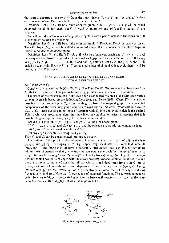
Lemma 3. Let (i) (G = (V, E), f : E + R, g : E + R) be a balanced graph;

(ii) C, = (e,, e2,. . . , ek) and C2 = (e;, el, . . . , eh) be two f, g-cycles with no common edges; (iii) C, and C, pass through a vertex v E V; (iv) any edge incidental u belongs to C, or C2.

Then C, and C, can be concatenated into one f, g-cycle. The outline of the proof is the following. Assume there are two pairs of adjacent edges

(e,, e,+,) and (e;, e;,,) belonging to C,, C,, respectively, incidental to u such that intervals [f(eJ, g(e,+,)) and [f(e&g(e;+,)) have a nonempty intersection (see, e.g. Fig. 6). Assuming without loss of generality that f(ei) of we can obtain one cycle by “jumping” from e, to e;,,, returning to v along C, and “jumping” back to C, from e; to e,+, (see Fig. 6). It is always possible to find two pairs of edges with the above property. Indeed, assume this is not true and there is a point t, and E > 0 such that all arrivals to u and departures from u in C, are in (-co, t,- E) and all arrivals to 2) and departures from u in C2 are in (t,+ E, x). Let f,, (respectively g,) be the restriction of f (respectively g) onto the set of edges entering (respectively leaving) u. Note that fO, g, is a pair of balanced functions. The corresponding local deficit function is I dfoYg(f). to is located in the interval between the earliest arrival to u and the latest departure from u. But 1 d,,,,(t,) = 0 which is impossible.0

Fig. 6. How to glue together two f, g-cycles.

466 I. GERTSBAKH and YURI GUREVICH

Theorem 1. Let (G = (V, E), f : E += R, g : E --) R) be a connected balanced graph. Then there is an f, g-Euler cycle.

Proof. By induction on #E. For #E = 0 it is obvious. Let the theorem be true for BE < n and consider a connected balanced graph with RE = n + 1. Take an arbitrary u,, E V and an edge e, coming out from uO. We want to construct an auxillary f, g-cycle containing e,. Let

(e,, e,, . . . , e,) be an f, g-path such that f ) {e E E: e enters v, ef ei, i < m} and g ({e E E: e leaves v, e # ei, 0 < i s m} are balanced for each u. e, enters some vertex u. By Corollary 2 there is always an edge e’ leaving u such that f 1 {e E E: e enters u, ef ei, i s m} and g 1 {e E E: e leaves u, ef e,, 1 c i s m, ef e’} remain balanced. If e’ f e,, define e,,, = e’ and proceed. Otherwise stop and the path C, = (e,, . . . , e,) is the desired auxillary f, g-cycle. If #C, = n + 1 the theorem is proved. Otherwise define E’ = E - Co, V’ = {v: u E V, u incidental to e E E’} and consider G’ = (V’, E’). It splits into connected components Gi = (Vi, E,), i = 1, . . . , k. It is easy toseethatforeachi=l,... , k f IEi and g (Ei are balanced on Gi. By the induction hypothesis there is an f, g-Euler cycle for each Gi, say Ci. There is a vertex u belonging to C,, and C, because G is connected. Now use Lemma 3 whose conditions are satisfied to concatenate C, with C,. Then concatenate Cz with C, U C,, etc. until an f, g-balanced Euler cycle is obtained.0

Theorem 1 suggests the following algorithm for constructing an f, g-Euler cycle. Construct an auxillary cycle C, and delete all its edges from G; for the remaining graph construct another auxiliary cycle C,, etc. Assume that a sequence Co, C,, . . . , C, is obtained until G gets exhausted. Then glue together C, with C,_, into one cycle, say CL_, using Lemma 3, glue together C;_, with Cr_2, etc. until all Ci will be concatenated into one f, g-Euler cycle.

3.2 Constructing a balanced Linis Graph Let us construct the Linis Graph LG(S) for the T-periodic schedule S. Our goal is to define

balanced functions f : E --* R, g : E + R representing the arrival/departure times. Let h be some hollow of hollow type ai of the deficit function d,(t) and I,,, J,, be the sets of

trips whose arrival and departure times, respectively, are located in h. Let to = min(p4: p E Iai}. For each p E I,, let us define the local arrival time at ai as p4* = p4- t, and for each q E J,,, let us define the local departure time from ai as 43* = q3 - t,. It is clear that if h,, h, are different hollows of hollow type ai and p&, p:,,,, are different trips of the same trip type pk with arrival (departure) times located in h,, h,, respectively, then their local arrival (departure) times are equal. Therefore, the local arrival/departure times are defined for each hollow type ai in a unique way. Define now I,,, J,, as the sets of trip-types whose arrival and departure times, respectively, are located in some hollow h of hollow type ai. Define functions fat: Ia, +R,

g, : J,, +R as follows: if pk E I,,, then fa,(pk) = pk4*; if qk E J4, then gaj(qk) = qk3*. Denote I = UaE4 UiIaty.J = UuEA Ui Jai and define f : I -+ R, g : J + R m such a way that their

restriction onto I,,, J,, coincide with f,,, goi. Clearly, f, g will be balanced on LG(S). The triple (LG(S) = (V, E), f : I + R, g : J + R) is a f, g-balanced graph termed a balanced Linis Graph.

3.3 Constructing regular chains Let us construct a balanced Linis Graph and a f, g-Euler cycle. Without loss of generality it

might be written in the following chain form

p’+p2+. . .-sp”, (3.1)

where pi is a trip-type. Each trip-type in S appears in (3.1) once and only once. Now construct an infinite periodic chain C” according to the following rules. (1) Take trip p,& (belonging to the i,th period on the periodic part of the deficit functions); let

p ,1,,,4 E h; join to p li ) the trip of trip-type p2 whose departure time is located in the same hollow h. Let this be trip p$. Clearly, p:i,,4 < p:i,,3 because (3.1) is an f, g-Euler cycle. Proceed until a trip of trip-type p” is picked. Denote the obtained sequence of trips by Cl’:

(3.2)

C,’ is a chain. We call it a master chain. Let p;,,,4 E h’. Consider the trip-type p’ departing from h’ and let it be p$,+,).

(2) Define

Homogeneous optimal fleet 467

(3.3)

and

p={c,“+czo~. . .~cp+c”,+,-~~~). (3.4)

Obviously, Co is a T-regular chain in S (see Subsection 1.2). Now obtain T- 1 additional T-regular chains in S, C’, . . . , CT-‘, where Ck ’ IS obtained from Co by adding the integer k to all lower indices of trips in Co, k = 1,. . . , T- 1:

ck={c,k+C?k+. . . + c,” +cf+,-. . .}, (3.5)

Crk=b:i,+k+T.r)+. “+PGn+k+7 r$. (3.6)

In this way we arrive at a set F” of T T-regular chains in S: F” = {Ci, 0 s i S T - 1). Their union is a schedule denoted So: So = U ;S,j C’. Clearly, (S-SO) is finite. We say that So contains almost all trips of S.

It is possible to add the trips in S-S’ to chains of F” “from the left” to obtain a fleet over S of size T. It can be done by extending to the left the chains in F” by adding to them the missing trips of S-SO (see Example 1). In this way we arrive at a system of chains F = {t”,OSkST- l}, where C” is obtained from Ck by extending it to the left. Clearly, F is a fleet over S and each chain in F is T-regular.

F will be termed a set of twin-type chains with respect to S or a twin-type fleet over S. CO, . . . , C?’ will

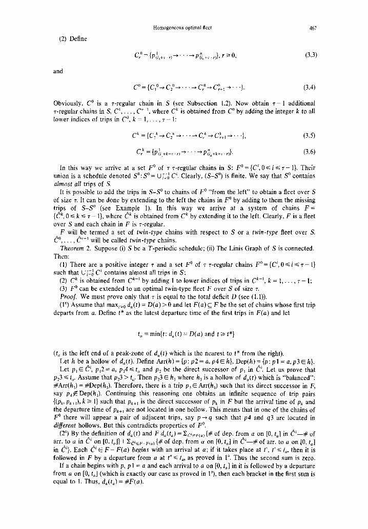
Proof. We must prove only that T is equal to the total deficit D (see (1.1)). (1”) Assume that max,,o d,(t) = D(a) > 0 and let F(a) G F be the set of chains whose first trip

departs from a. Define t* as the latest departure time of the first trips in F(a) and let

t, = min{t: d,(t) = D(a) and t 2 t*}

(t, is the left end of a peak-zone of d,(t) which is the nearest to t* from the right). Let h be a ,hollow of d,(t). Define Arr(h) = {p: p2 = a, p4 E h}, Dep(h) ~,{p: p 1 = a, p3 E h}. Let p, E C’, p,2 = a, p,4 G t, and pZ be the direct successor of p, in C’. Let us prove that

p,3 < t,. Assume that p,3 > t,. Then p,3 E h, where h, is a hollow of d,(t) which is “balanced”: #Arr(h,) = #Dep(h,). Therefore, there is a trip pj E Arr(h,) such that its direct successor in F, say p4f! Dep(h,). Continuing this reasoning one obtains an infinite sequence of trip pairs

bk, Pk+,h k 2 1) such that Pk+l is the direct successor of pk in F but the arrival time of pk and the departure time of p k+i are not located in one hollow. This means that in one of the chains of F” there will appear a pair of adjacent trips, say p +q such that p4 and q3 are located in diferent hollows. But this contradicts properties of F”.

(2”) By the definition of d,(t) and F d,(t,) = X~iEFcoj {# of dep. from a on [0, t,] in Ci-# of arr. to a in Ci on [0, t,]} + ~~~~~~~~~~ {# of dep. from (Y on [O, t,l in C’-# of arr. to a on [0, t,] in Ci}. Each di E F-F(a) begins with an arrival at a; if it takes place at t’, t’ < t,, then it is followed in F by a departure from a at t” s t,, as proved in 1”. Thus the second sum is zero.

If a chain begins with p, p 1 = a and each arrival to a on [O, t,] in it is followed by a departure from a on [0, t,] (which is exactly our case as proved in l”), then each bracket in the first sum is equal to 1. Thus, d,(t,) = #F(a).

468 I. GERTSBAKH and YURI GUREVICH

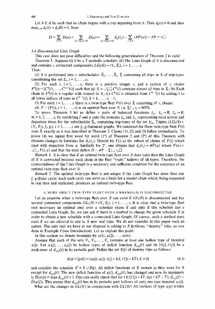
Let b E A be such that no chain begins with a trip departing from b. Then dh(f) s 0 and thus maxtsO d,,(t) = d,,(O) = 0. Now

D= c, D(a)= x D(a)= 2 d,(t,)= x (#F(a))= #F= 7.0 CIEA (a: D(o)>O) (a. D(a)>O) LIEA

3.4 Disconnected Linis Graph This case does not pose difficulties and the following generalization of Theorem 2 is valid: Theorem 3. Suppose (i) S be a T-periodic schedule; (ii) The Linis Graph of S is disconnected

and contains s connected components LG,(S) = (Vi, Ei), i = 1,. . . , s. Then:

(1) S is partitioned into s subschedules s,, . , S,, Si containing all trips in S of trip-types constituting the set Ei, i = 1, . . . , s ;

(2) For each i, i=l,... , s, there is a positive integer 7i and a system of 7i chains F’(i) = {C”(i), . . . , P-‘(i)} such that (a) Si = U>:A Ck(i) contains almost all trips in $; (b) Each chain in F’(i) is Ti-regular with respect to Si; (c) Ck(i) is obtained from Ckm’(i) by adding 1 to all lower indices of trips in Ck-l(i), k = 1,. . . , q - 1;

(3) For each i = 1,. . , s there is a twin-type fleet F(i) over $ consisting of ~~ chains; (4) F = {F(i), i = 1,. . . , S} iS an Optid fleet OVer s, i.e. z;=, Ti = MFS.

To prove Theorem 3 let us define s pairs of balanced functions f,,,: I,,, + R, J, + R, m = 1,2,. . . , s, by restricting f and g onto the domains I,,, and J,,, representing local arrival and departure times for the subschedule $,, containing trip-types of the set E,. Triples (LG,(S) =

(Vi, Ei), .fi, gi), i = 1,. . ( , s are fi, g-balanced graphs. We construct for them twin-type fleet F(i) over Si exactly as it was described in Theorem 2. Claims (l), (2) and (3) follow immediately. To prove (4) we repeat first word for word (1”) of Theorem 2 and (2”) of this Theorem with obvious changes in formulas for d,(t,). Denote by F(i, a) the subset of chains of F(i) which start with departure from a. Similarly for 2”, one obtains that d,(t,) = #F(a) where F(a) = U I=, F(i, a) and that the total deficit D = #F = Xl=, T~.O

Remark 1. It is clear that if an optimal twin-type fleet over S does exist then the Linis Graph of S is connected because each chain in the fleet “visits” hollows of all types. Therefore, the connectedness of the Linis Graph is a necessary and sufficient condition for the existence of an optimal twin-type fleet over S.

Remark 2. The optimal twin-type fleet is not unique if the Linis Graph has more than one f, g-Euler cycle: each such cycle can serve as a basis for a master chain which, being expanded

in real time and replicated, produces an optimal twin-type fleet.

4. MORE ABOUTTWIN-TYPE FLEET OVER S WHENGL(S)IS DISCONNECTED

Let us examine when a twin-type fleet over S can exist if GL(S) is disconnected and has several connected components GL,(S) = (Vi, E,), i = 1, . . . , s. It is clear that a twin-type fleet (not necessary an optimal one) over a schedule exists if and only if this schedule has a connected Linis Graph. So, we can ask if there is a method to change the given schedule S in order to obtain a new schedule with a connected Linis Graph. Of course, such a method does exist if we are allowed to add to S new real trips. We do not consider in this paper such an option. The only tool we have at our disposal is adding to S fictitious, “dummy” trips, as was done in Example 1 (see Introduction). Let us explain this point.

In this section we denote terminals by a(l), a(2), . . . , a(m). Assume that each of the sets V,, VZ, . . . , V, contains at least one hollow type of terminal

a(j). Let a,(j), . . . , a,(j) be hollow types of deficit function daci,(t) and let [t(j), t’(j)] be a peak-zone of dacj,(t) in its periodic part. Define the set S(j) of dummy trips as follows:

S(i) = b(k) = (a(i), a(i), t(i) + kT, W + W, k 2 01 (4.1)

and consider the schedule S’ = S U S(j). All deficit functions of S’ remain as they were for S except for d&t). The new deficit function of a(j), dacj,(t), has changed and now its maximum is &a(j)) = max dacj,(t) + 1. One can easily check that for t E [t’(j) + kT, t(j) + kT + T), d,,j,(t) < &a(j)). This means that dacj,(t) has in its periodic part hollows of only one type denoted a,(j).

What are the changes in GL(S’) in comparison with GL(S)? All vertices of type ai within

Homogeneous optimal fleet 469

G&(S) are replaced by vertex a,(j); each edge e E Ei from a,(j) E Vi to u E Vi is replaced by edge from a,(j) to v. The new subgraphs of GL(S’) corresponding to GLr(S), i = 1,. . . , r will have now one common vertex a,(j) and will form one connected component in GUS’); the sets

V,, V,, ’ . , V, now are “glued” together. So, we have a tool to glue together connected components of the disconnected Linis Graph.

Assume that p + w + q is a fragment of some chain in the fleet over S’ where p, q E S and w is a dummy trip. “To carry out” w means that a vehicle arrived in p2 at time p4 must remain in terminal p2 until time q3. S’ is essentially the same schedule S; adding dummy trips to S means only increasing the time spent by vehicles in terminals. More formally, adding S(j) to S forces us to build chains by overlapping some peak-zones of the deficit functions of the schedule S, which is, in fact, a violation of rules for constructing an optimal fleet over S.

Now we need to define an oriented graph called the graph of terminals. Definition. The graph of terminals of schedule S, GT(S) is a finite oriented graph GT(S) =

(V, E) where the vertices are terminals and the edges are trip-types; if trip e = (a(j), a(k), e3, e4) E S is of trip-type e, E E then the edge e, comes out from vertex a(j) and enters vertex a(k).

Now define a set B C A, B = {a(i): d&t) has more than one hollow type}. For each a(r) E B define the corresponding sequence of dummy trips S(r), similar to (4.1) and consider a new schedule S* = S U (lJfOcrjEBI S(r)). Its Linis Graph is GUS*) = (V, E), where V is the set of terminals and E is the set of trip-types of S*. The only difference between GUS*) and GT(S) is that in GL(S*) there are loop-type edges from a(i) to a(i), a(i) E B, created by dummy trip-types. Therefore, GL(S*) is connected if and only if GT(S) is connected. Therefore, there is a way to obtain a twin-type fleet over S iff GT(S) is connected.

From now on let GT(S) be connected. One can look for a most economic way to complement S by sets of dummy trips. This is illustrated by the following.

Example 2. Let GL(S) have three connected components GLi(S) = (Vi, Ei), i = 1, 2, 3, and V, = {a,(l), a,(2)}, V, = {a,(l), a,(2), a,(3)}, V, = {aJl), a,(3)}. If we add to S the sequence S(2) then V, and Vz are glued together; adding S(3) will result in a connected Linis Graph. On the other hand, adding only one sequence of dummy trips S(1) would immediately lead to a connected Linis Graph.

In most practical problems the Linis Graph has not too many components and the smallest set of dummy trips can be found easily by means of a simple enumeration. Note that the set of potential candidates for T* can be reduced by excluding terminals which appear in only one component of the Linis Graph.

Assume that adding Q dummy trip types in terminals {a(i$), . . . , n(r#} = A(Q) provides a connected Linis Graph and there is no other set of terminals of smaller size with the same property. We call A(Q) the core set. In example 2 A(Q) = {a(l)}.

The above discussion can be summarized in the following Theorem 4. Suppose (i) S is a T-periodic schedule; (ii) GT(S) is connected; (iii) GL(S) is

disconnected; (iv) The core set of the Linis Graph of S is {a(l), . . . , a(Q)}. Then the optimal twin-type fleet over S contains D + Q twin-type chains.

Proof. For each terminal a(j) in the core set define the sequence of dummy trips (4.1) where [t(j), t’(j)] is a peak zone of the deficit function d,(j,(t) in its periodic part. Consider the schedule

S* = S U (jt, S(j)). (4.4)

By the definition of the core set, the Linis Graph of S* is connected. Then by Theorem 2 it allows construction of a twin-type fleet whose size is equal to the total deficit of S*, D+ Q. It

follows from the definition of the core set that the minimal number of sequences of dummy trips added to S in order to obtain a schedule with a connected Linis Graph is Q. Thus, the fleet of size D + Q is optimal along all twin-type fleets over SO

5. CONCLUDING REMARKS: THE CENTER PROBLEM; ADDING TRIPS

TO THE SCHEDULE.

The following problem is of interest for planning transportation systems (see Gertsbach and Gurevich (1977), Section 3.2). Assume that there is a set of terminals A* called center. It is

T&B Vol. 16, No. 6-D

470 1. GERTSBAKH and YURI GUREVICH

necessary to construct a fleet of minimal size having the following property: each chain in the fleet must go through a terminal belonging to the center.

If there are connected components of the Linis Graph which do not contain representatives of A*, then one can try to use the dummy trip technique (see Section 4) to glue such components to those which contain representatives of the center set. If it is possible to obtain a new Linis Graph with center representatives in each of its connected component then a fleet satisfying the center property can be found.

It can be said that the center problem may have no solution at all if the graph of terminals is disconnected. An example is GL,(S) = (Vi, E,), i = 1, 2, V, = {a,, a,, b,}, VZ = {c,, c2, e,}. A* = {a, b}. It is clear, that it is not possible to obtain any fleet which would contain chains visiting terminals a, c, e, b. Of course, such chains could be obtained if we were allowed to add new trips to the original schedule, say from a to c and from c to a, thus providing a connection between components of the Linis Graph. Here we enter a new circle of problems connected with adding real trips to the schedule. We will make only some brief remarks.

Adding new trips can give many surprising results which might be classified into two main groups: changing the fleet size, including the decrease of it; changing the structure of the optimal chain decomposition. The only work in this area we know is a paper of Ceder and Stern (1982) in which the influence of adding deadheading trips on the fleet size has been investigated for a nonperiodic schedule.

Remark. In November 1981 we became aware about the existence of a recent paper by Linis and Maksim (1980), “The number of transportation units needed for a schedule”, published in Moldavian Math. Collection (in Russian). Independently of us, Linis and Maksim obtained some of the results presented in this paper and, in particular, a theorem which is similar to our Theorem 1.

REFERENCES

Bartlett T. E. (1957) An algorithm for the minimum number of transport units to maintain a fixed schedule, Nat. Res. Log. Quart. 4, 139-149.

Berge C. (1958) Theorie des graphes el ses applications. Dunod, Paris. Ceder A. and Stern I. (1982) Deficit function procedure for bus scheduling with dead-heading trip insertion for fleet-size

reduction. Transpn. Sci. 16. Gertsbach I. and Gurevich Yu. (1977) Constructing an optimal fleet for a transportation schedule. Transpn. Sci. 11, 20-36. Linis V. K. and Maksim M. S. (1967) On the problem of constructing routes. Proc. Instit. Civil Aviation. 102, 3645 (in

Russian). Salzborn F. J. M. (1974) Minimum fleet size models for transportation systems. Transpn. and Trajic Theory (Edited by

Buckley, D. J.), Proc. 6th Int Symp. of Transpn. and Trajfc Theory, Sydney.