Homological Methods for the Economic Equilibrium Existence

Problem: Coincidence Theorem and an Analogue of Sperner’s

Lemma in Nikaido (1959) ∗

Ken Urai

Graduate School of Economics

Osaka University

Abstract

In this paper, I introduce the theorems in Professor Hukukane Nikaido’s work, “Coincidence

and some systems of inequalities,” published in the Journal of Mathematical Society of Japan,

1959, and note the significance of his mathematical methods on the history and the future of

mathematical economics. Nikaido (1959) may be considered a compilation of his works of the

1950’s on economic equilibrium existence problems. It also provides, however, his further devel-

opments and attempts for mathematical methods in the theory of mathematical economics and

an algebraic (algebraic topological) methods based on results of the Vietoris homology theory

(the earliest kind of Cech-type homology theories). From Nikaido’s main mathematical results,

an analogue of Sperner’s lemma and a coincidence theorem, we may obtain a simple proof for

Eilenberg-Montgomery’s theorem for finite dimensional cases. We may also utilize such homo-

logical methods for many generalizations of fixed point arguments on multivalued mappings in

relation to Lefschetz’s fixed point theorem.

Keywords : Fixed point theorem, Existence of equilibrium, Cech homology theory, Vietoris

homology theory, Browder’s fixed point theorem, Kakutani’s fixed point theorem, Lefschetz’s

fixed point theorem.

JEL classification: C60; C62; C70; D50

1 Introduction

In this paper, I introduce the theorems in Professor Hukukane Nikaido’s work, “Coincidence and some systems

of inequalities,” published in the Journal of Mathematical Society of Japan, 1959, and note the significance

of his mathematical methods on the history and the future of mathematical economics. Nikaido (1959)

may be considered a compilation of his works of the 1950’s on economic equilibrium existence problems. It

∗The manuscript is prepared for the special session of Nikaido Conference at Hitotsubashi University on March 18 and 19,2006. Contents in Sections 2 – 6, except for the proof of Sperner’s lemma (Lemma 4.4), arguments for class B (Browder type)mappings in Section 5, and several additional figures, have been taken from Chapter 6 of my Ph.D thesis (Urai, 2005).

also provides, however, his further developments and attempts for mathematical methods in the theory of

mathematical economics and an algebraic (algebraic topological) methods based on results of the Vietoris

homology theory (the earliest kind of Cech-type homology theories). From Nikaido’s main mathematical

results, an analogue of Sperner’s lemma and a coincidence theorem, we may obtain a simple proof for

Eilenberg-Montgomery’s theorem for finite dimensional cases. We may also utilize such homological methods

for many generalizations of fixed point arguments on multivalued mappings in relation to Lefschetz’s fixed

point theorem.

As is well-known, Professor Nikaido was a great mathematician as well as an outstanding social scientist.

He had a special viewpoint on mathematical methods for the social sciences that view mathematics not as

a simple tool but as a language. Therefore, for him, mathematical economics is not a simple description of

the world using mathematical concepts but a study of the world through the language (or methods) of the

mathematician.

With each mathematical theory is associated a different way of analyzing the world. For example, there

is an important difference between the differentiable approach (research based on differential calculus) and

an approach based merely on set theoretical and/or algebraic methods in mathematical economics. Since

the concepts and methods of differential calculus are based on the theory of sets and/or algebra, the former

includes analytic works that result from seeing the world as a differentiable object, and the latter include

synthetic attempts or methods to construct models that are more appropriate to describe our real world.

The results of the former are always based on the concept of differentiability so that it is more desirable to

reexamine them under more primitive concepts, like finiteness, sequences, or limits under the set theoretical

and/or algebraic methods.

In this sense, it is always significant for the theory of mathematical economics to use more primitive

mathematical concepts together with more general or fundamental mathematical methods. Methods in

mathematical economics in the 1950’s and 1960’s based on rigorous set theoretical arguments and general

topology, e.g., Debreu (1959), Nikaido (1968), etc., have, therefore, important meaning for the history of

social science as a new basic (fundamental) language for describing the society.

I introduce here some of the most general (and fundamental) theorems of Professor Nikaido from that era,

an analogue of Sperner’s lemma and a theorem for the coincidence of mappings (Nikaido, 1959; Lemma 1,

Theorem 3). The analogue of Sperner’s lemma may be considered to represent the essential part of fixed

point or coincidence theorems in finite dimensional vector spaces, as does Sperner’s lemma. The lemma

may be useful as a proof of the theorem on coincidence points of mappings on general compact Hausdorff

spaces with or without vector space structure. The result may also be directly used for economic equilibrium

problems on general compact Hausdorff spaces. Arguments are based on an abstract homology theory of the

Cech-type that is founded on more primitive algebraic concepts than the singular homology theory.

2 Vietoris and Cech Homology Groups

Let X be a compact Hausdorff space. Cover(X) denotes the set of all finite open coverings ofX . Remember

that for each covering M,N ∈ Cover(X), we write N4 M if N is a refinement of M and M4∗ M if N

is a star refinement of M (Figure 1). It is also important to recall that for each covering M ∈ Cover(X),

covering N ∈ Cover(X) such that N4∗ M exists, hence relation 4 directs set Cover(X). Since this is a

crucial property, I will write down here a simple sketch of a direct proof for our special case, though the

result may be seen in the literature, e.g., Tukey (1940; p.47).

2

Figure 1: Star Refinements

Lemma 2.1 : Let X be a compact Hausdorff space. For each covering M ∈ Cover(X), a star refinement

N ∈ Cover(X) of M, N4∗ M, exists

Proof : Suppose that X is covered by family M{M1, . . . ,Mm} (m ≥ 2). First we can see under the

condition of normal space that M1 and M2 include closed sets C1 and C2 respectively, together with open sets

U1 ⊂ C1 and U2 ⊂ C2 such that X ⊂ U1∪U2∪⋃

i≥3 Mi. It is clear that family N2 = {U1∩M2, U2∩M1,M1 \

C2,M2 \C1} satisfies ∀N ∈N2, the star of N in N2, St(N,N2) =⋃{N ′|N ∩N ′ 6= ∅, N ′ ∈N2} is a subset

of M1 or M2, and N2 ∪ {M3, . . . ,Mm} is a covering of X . Next assume that for covering {M1, . . . ,Mn−1},

family Nn−1 exists such that ∀N ∈ Nn−1, the star of N in Nn−1, St(N,Nn−1) is a subset of Mi for some

i = 1, . . . , n − 1, and Nn−1 ∪ {Mn,Mn+1, . . . ,Mm} is a covering of X . Then for Mn, (again under the

condition of normal space,) we may chose subsets Vn ⊂ Dn ⊂ Un ⊂ Cn of Mn such that Vm and Um are

open, Dm and Cm are closed, and Nn−1 ∪ {Vn,Mn+1, . . . ,Mm} is a covering of X (Figure 2). Define Nn

as Nn = {N \ Cn|N ∈ Nn−1} ∪ {N ∩Mn \Dn|N ∈ Nn−1} ∪ {Un}. It is easy to verify that Nn satisfies

Figure 2: Construction of a Star Refinement

that ∀N ∈Nn, the star of N in Nn is a subset of Mi for some i = 1, . . . , n, and Nn ∪ {Mn+1, . . . ,Mm} is a

covering of X . Since the process may be continued to n = m, we may obtain a star refinement of M. �

3

Cech Homology

The nerve of the covering M of X , Xc(M), is an abstract complex such that the set of vertices of Xc(M)

is M and n-dimensional simplex σn = M0M1 · · ·Mn belongs to Xc(M) if and only if⋂n

i=0Mi 6= ∅. We

call an n-dimensional simplex σn in Xc(M) an n-dimensional Cech M-simplex, (or simply, Cech simplex,

n-dimensional Cech simplex, Cech M-simplex, etc., as long as there is no fear of confusion). X c(M) is also

called the Cech M-complex. In the following, we assume that every Cech M-complex is oriented. Since

M is a finite covering, we may identify Xc(M) with a polyhedron (a realization) in a finite dimensional

Euclidean space.

If p : N→M is a mapping such that for all N ∈ N, N ⊂ p(N) ∈M, we say that p is a projection. It is

clear that if N is a refinement of M, then for each N1, N2 ∈N, N1∩N2 6= ∅ implies that p(N1)∩p(N2) 6= ∅.

Hence, the vertex mapping, projection p, induces uniquely a simplicial map X c(N) 3 N1N2 · · ·Nk 7→

p(N1)p(N2) · · · p(Nk) ∈ Xc(M) which is also denoted by p and called a projection.

An n-dimensional Cech M-chain, cn, is an entity which is represented uniquely as a finite sum of Cech

M-simplexes,

cn =k∑

i=1

αiσni , (σn

1 , . . . , σnk ∈ X

c(M)),

where coefficients α1, . . . , αk are taken in a field F . The set of all n-dimensional Cech M-chains, Ccn(M),

may be identified, therefore, with the vector space over F spanned by elements of the form 1σn, where σn

runs through the set of all n-dimensional Cech M-simplexes.

Let us consider the boundary operator among chains, ∂n : Ccn(M)→ Cc

n−1(M), for each n, as usual, i.e.,

the linear mapping,

∂n : M0M1 · · ·Mn →n∑

i=0

(−1)iM0M1 · · · Mi · · ·Mn,

where the series of vertices with a circumflex over a vertex means the ordered array obtained from the

original array by deleting the vertex with the circumflex and for all n < 0, it is supposed that Ccn(M) =

0. Then, the set of all n-dimensional Cech M-cycles, Zcn(M), and the set of n-dimensional Cech M-

boundaries, Bcn(M), may be defined as usual, so that we obtain the n-th Cech M-homology group, Hc

n(M),

for each n. For each N 4M and dimension n, simplicial map p induces chain homomorphism pMN

n so

that (Cvn(M), pMN

n )M,N∈Cover(X), (Zvn(M), pMN

n )M,N∈Cover(X), and (Bvn(M), pMN

n )M,N∈Cover(X), form inverse

systems.

Note that if N 4M, and if p : N → M and p′ : N → M are projections, two simplicial maps,

p and p′, are contiguous, i.e., for each Cech N-simplex, N0N1 · · ·Nk, images p(N0)p(N1) · · · p(Nk) and

p′(N0)p′(N1) · · · p′(Nk) are faces of a single simplex.1 Since two contiguous simplicial maps are chain homo-

topic,2 p and p′ induce the same homomorphism, pMN

∗n : Hcn(N) → Hc

n(M) for each n. The limit for the

inverse system, (Hcn(M), pMN

∗n ), on the preordered family, (Cover(X),4),

Hcn(X) = lim←−

M

Hcn(M),

is the n-dimensional Cech Homology group.

1Indeed, it is clear that the intersection (⋂k

i=0p(Ni)) ∩ (

⋂k

i=0p′(Ni)) ⊃

⋂k

i=1Ni 6= ∅. Hence, the array obtained by

deleting all of the second occurence for the same vertex from the series, p(N0)p(N1) · · · p(Nk)p′(N0)p′(N1) · · · p′(Nk), is a CechM-simplex.

2See for example Eilenberg and N.Steenrod (1952; p.164). If we are allowed to define piecewise linear extensions p and p′ ofp and p′, respectively, it may also easy to find a homotopy bridge among p and p′.

4

Under the definitions of the homology group and the inverse limit, an element ofH cn(X) may be considered,

intuitively, as an equivalence class of a sequence of Cech cycles, {zn(M) ∈ Zcn(M) : M ∈ Cover(X)},

such that for each M,N ∈ Cover(X) satisfying that N 4M, we have zn(M) ∼ pMN

n (zn(N)), where the

equivalence relation is defined relative to the class of Cech boundaries, i.e., zn(M)−pMN

n (zn(N)) ∈ Bcn(M).3

Vietoris Homology

An n-dimensional Vietoris simplex is a collection of n + 1 points of X , x0x1 · · ·xn. A Vietoris simplex,

σ = x0x1 · · ·xn, is said to be an M-simplex if the set of vertices, {x0, x1, . . . , xn}, is a subset of an element

of M. The set of all Vietoris M-simplexes forms a simplicial (infinite) complex (Vietoris M-complex) and

is denoted by Xv(M). An orientation for n-dimensional Vietoris simplex x0x1 · · ·xn is a total ordering on

{x0, x1, . . . , xn} up to even permutations. In the following we suppose that every Vietoris M-complex is

oriented.

The set of all n-dimensional Vietoris M-chain, Cvn(M), is the vector space whose elements are uniquely

represented as a finite sum of n-dimensional Vietoris M-simplexes,

cn =

k∑

i=1

αiσni , (σn

1 , . . . , σnk ∈ X

v(M)),

where coefficients α1, . . . , αk are taken in a field F . We may also consider the boundary operator among

chains, ∂n : Cvn(M)→ Cv

n−1(M), for each n, as the linear map satisfying,

∂n : x0x1 · · ·xn →n∑

i=0

(−1)ix0x1 · · · xi · · ·xn,

where the circumflex over a vertex means the elimination as before, and it is supposed that Cvn(M) = 0 for

all n < 0. The set of all n-dimensional Vietoris M-cycles, Zvn(M), and the set of n-dimensional Vietoris

M-boundaries, Bvn(M), may also be defined as usual, so that we obtain the n-th Vietoris M-homology

group, Hvn(M), for each n.

For coverings M,N ∈ Cover(X), it is clear that (N 4M) =⇒ (Xv(N) ⊂ Xv(M)). Denote by hMN

n :

Cvn(N) → Cv

n(M) the chain homomorphism induced by the above inclusion. Then, for each n, the system

of vector spaces with mappings, (Cvn(M), hMN

n )M,N∈Cover(X), their cycles, (Zvn(M), hMN

n )M,N∈Cover(X), and

boundaries, (Bvn(M), hMN

n )M,N∈Cover(X), form inverse systems. The inverse limit of the inverse system,

(Zvn(M)/Bv

n(M), hMN

∗n )M,N∈Cover(X),

Hvn(X) = lim←−

M

Hvn(M),

is the n-dimensional (n-th) Vietoris Homology group.

An element of Hvn(X) may be identified with an equivalence class of a sequence of n-dimensional Vietoris

M-cycles, M ∈ Cover(X), (an n-dimensional Vietoris cycle), {zn(M) ∈ Zvn(M)|M ∈ Cover(X)}, such that

for each M,N ∈ Cover(X) satisfying that N 4M, we have zn(M) ∼ hMN

n (zn(N)), where the equivalence

class is taken with respect to Vietoris M-boundaries, i.e., zn(M)− hMN

n (zn(N)) ∈ Bvn(M).4

3For more details of the Cech homology theory, see Eilenberg and N.Steenrod (1952). For more introductory arguments,Hocking and Young (1961; Chapter 8) is also recommended.

4The concept of Vietoris homology group was originally introduced by Vietoris (1927) as the first homology theory of theCech type for metric spaces. Though the theory has been used in many researches, e.g., Eilenberg and Montgomery (1946), ithas not been frequently discussed as has the more general Cech theory. The theory was extended to be applicable for cases ofcompact Hausdorff spaces by Begle (1950), and the result was used in Nikaido (1959) to prove an analogue of Sperner’s lemma.

5

Vietoris and Cech Cycles

The Cech homology theory is a powerful tool to approximate the space with groups of a finite complex.

The Vietoris homology theory, on the other hand, has an intuitional advantage that we may characterize the

space directly by its elements (points). Fortunately, we may utilize both merits since the two homological

concepts give the same homology groups (see Theorem 2.3 below).

Before proving this, let us see the following facts on equivalences of two cycles on a simplicial complex. Since

a homology group is nothing but a set of equivalence classes of cycles, it is not surprising that homological

arguments often depend on this type of equivalence results. Let K be a simplicial complex. Suppose that

the set of vertices of K, Vert(K), is simply ordered in an arbitrary way, and let σn = 〈a0, a1, . . . , an〉 be an

n-simplex (oriented by the simple order) in K. The product simplicial complex of K and the unit interval

denoted by K×{0, 1} is the family of simplexes of the form 〈(a0, 0), (a1, 0), . . . , (ai, 0), (ai, 1), . . . , (an, 1)〉 for

each 〈a0, a1, . . . , an〉 ∈ K together with all their faces (Figure 3). The subcomplex of K×{0, 1} constructed

Figure 3: Prism K × {0, 1}

by all simplexes of the form 〈(a0, 0), . . . , (an, 0)〉 may clearly be identified with K and is called the base of

K × {0, 1}. There also exists an isomorphism between K and the subcomplex of all simplexes of the form

〈(a0, 1), . . . , (an, 1)〉, which is called the top of K × {0, 1}. For each n-simplex 〈σn〉 = 〈a0, . . . , an〉 of K,

define an n+ 1-chain, Φn(σn), on product simplicial complex K × {0, 1} as

Φn(σn) =

n∑

j=0

(−1)j〈(a0, 0), . . . , (aj , 0), (aj , 1), . . . , (an, 1)〉.(1)

Extend each Φn to a homomorphism on Cn(K) to Cn(K × {0, 1}). Then we can verify through direct

calculations that for each n-chain cn ∈ K,

∂n+1Φn(cn) + Φn−1∂n(cn) = cn × 1− cn × 0 ∈ Cn−1(K × {0, 1}),(2)

where cn×1 (resp., cn×0) is the chain on the top (resp. base) of K×{0, 1} formed by replacing each vertex

of each simplex of cn by the vertex of the ordered pair with 0 (resp., 1). Hence, if zn is a cycle on K,

∂n+1Φn(zn) = zn × 1− zn × 0 ∈ Bn(K × {0, 1}),(3)

i.e., we have zn × 0 ∼ zn × 1 on K × {0, 1}. Therefore, if there exists a simplicial mapping ψ on K × {0, 1}

to a certain simplicial complex L, the next lemma holds.

6

Lemma 2.2 : Assume that there is a simplicial mapping ψ on K × {0, 1} to a simplicial complex L. For

two images ψq+1(zq × 0) and ψq+1(z

q × 1) in the q-th chain group Cq(L) of q-cycle zq ∈ Cq(K) (through the

induced homomorphism ψq+1 : Cq+1(K × {0, 1})→ Cq(L)), we have ψq+1(zq × 0) ∼ ψq+1(z

q × 1) on L.

We now see the following fundamental result.

Theorem 2.3 : (Begle 1950a) Let X be a compact Hausdorff space. The q-th Vietoris homology group,

Hvq (X), is isomorphic to the corresponding Cech homology group, Hc

q (X), for each q.

To show the above result, use the following two simplicial mappings.5 Given covering M in Cover(X), chose

refinement N 4∗ M, which is always possible for a compact Hausdorff space by Lemma 2.1. It is convenient

for the discussion below to denote one of such selections for each M by a fixed operator on Cover(X) as

N = ∗M.6 For each M ∈ Cover(X) and for each x ∈ X , there are Nx ∈ ∗M and Mx ∈M such that x ∈ Nx

and St(Nx; ∗M) ⊂Mx. Moreover, for each N ∈ ∗M there is an element xN ∈ N . Define functions ζbM

and

ϕbM

as

ζbM

: Vert(Xv(∗M)) = X 3 x 7→Mx ∈M = Vert(Xc(M))(4)

ϕbM

: Vert(Xc(∗M)) = ∗M 3 N 7→ xN ∈ X = Vert(Xv(M))(5)

Under the definition of star refinement, it is easy to see that ζbM

and ϕbM

are simplicial mappings. Hence,

we obtain chain homomorphisms ζbMq : Cv

q (N) → Ccq (M) and ϕb

Mq : Ccq (M) → Cv

q (P). As we see below,

these mappings play essential roles in characterizing relations between Vietoris and Cech homology groups.

Especially, mappings ζbMq and ϕb

Mq induces, respectively, isomorphisms ζb∗q : Hv

q (X) → Hcq (X) and ϕb

∗q :

Hcq (X)→ Hv

q (X) (Theorem 2.3), and ϕbMq ◦ζ

bNq (N = ∗M) assures the finite dimensional character of acyclic

spaces (Theorem 3.2) or locally connected spaces (Theorem 3.4).

Proof of Theorem 2.3 : Let γq = {γq(N)|N ∈ Cover(X)}, (or simply, {γq(N)}) be an q-dimensional

Vietoris cycle. For each M ∈ Cover(X) and N = ∗M, define zq(M) as zq(M) = ζbMq(γ

q(N)). We see (1)

that zq = {zq(M)} is a Cech cycle and (2) that the mapping ζb∗q : γq 7→ zq is an isomorphism on Hv

q (X) to

Hcq (X).

(1) Since ζbMq : Cv

q (N) → Ccq (M) is a chain homomorphism, all zq(M) (M ∈ Cover(X)) are cycles in

Ccq (M). Hence, by definition of inverse limit, all we have to show is zq(M1) ∼ pM1M2

q (zq(M2)) for each

M2 4M1. Let N1 and N2 be refinements of M1 and M2, respectively, to define mappings ζbM1q and

ζbM2q . By Lemma 2.1, we can take P as P 4∗ N1 and P 4∗ N2. Note that since {γq(N)} is a Vietoris

cycle, we have hN1P

q (γq(P)) ∼ γq(N1) and hN2P

q (γq(P)) ∼ γq(N2). Hence, zq(M1) = ζbM1q(γ

q(N1) ∼

ζbM1q(h

N1P

q (γq(P))) and pM1M2

q (zq(M2)) = pM1M2

q (ζbM2q(γ

q(N2)) ∼ pM1M2

q (ζbM2q(h

N2P

q (γq(P))).7 It follows

that all we have to show is ζbM1q(γ

q(P)) ∼ pM1M2

q (ζbM2q(γ

q(P)). Let K = K(γq(P)) be the complex consists

of all simplexes in cycle γq(P) together with their faces. Then by Lemma 2.2, it is sufficient to show the

existence of simplicial map ψ on K×{0, 1} to L = Xc(M1) such that ζbM1q(γ

q(P)) and pM1M2

q (ζbM2q(γ

q(P))

are images through the induced map ψq+1 : Cq+1(K × {0, 1}) → Xc(M1) of γq(P) × 0 and γq(P) ×

1, respectively. For each a ∈ Vert(K), define ψ as ψ((a, 0)) = ζbM1

(a) and ψ((a, 1)) = pM1M2ζbM2

(a).

For any simplex 〈(a0, 0), . . . , (ai, 0), (ai, 1), . . . , (ak, 1)〉 in K × {0, 1}, we have a simplex a0 · · · ak of K =

5These mappings are defined by Begle (1950a).6For this, Axiom of Choice is needed.7In the above, inclusion mappings hN1P

q and hN2Pq might be abbreviated. Since including relation Cv

q (N') ⊂ Cvq (N) for

each N'4N is obvious, these operators will be omitted henceforth as long as there is no fear of confusions.

7

K(γq(P)), so that there exists P ∈ P, a0, . . . , ak ∈ P . We have to show that 〈ζbM1

(a0), . . . , ζbM1

(ai),

pM1M2ζbM2

(ai), . . ., pM1M2ζbM2

(ak)〉 forms a simplex inXc(M1). For each j, 0 ≤ j ≤ i, since P 4∗ N1 4∗ M1,

each ζbM1

(aj) = M1aj(0 ≤ j ≤ i) includes St(N1aj

,N1) for a certain N1aj3 aj . Hence, P which has

aj and satisfies St(P,P) ⊂ N1 for a certain N1 ∈ N1 must be a subset of St(N1aj,N1) ⊂ M1aj

. For

each j, i ≤ j ≤ k, since P 4∗ N2 4∗ M2 4 M1, each pM1M2ζbM2

(aj) = pM1M2M2aj(i ≤ j ≤ k) includes

St(N2aj,N2) for a certain N2aj

3 aj . Hence, P which has aj and satisfies St(P,P) ⊂ N2 for a certain

N2 ∈ N2 must be a subset of St(N2aj,N2) ⊂ M2aj

so that the corresponding element under projection

pM1M2

0 of M1. Therefore, we have ζbM1

(a0) ∩ . . . ∩ ζbM1

(ai) ∩ pM1M2ζbM2

(ai) ∩ pM1M2ζbM2

(ak) ⊃ P 6= ∅

and 〈ζbM1

(a0), . . . , ζbM1

(ai), pM1M2ζb

M2(ai), . . . , p

M1M2ζbM2

(ak)〉 ∈ Xc(M1), i.e., ψ is a simplicial map. By the

construction of induced map ψq , it is also clear that ψq+1(γq×0) = ζb

Mq(γq) and ψq+1(γ

q×1) = pMN

q ζbNq(γ

q).

(2) We have to show that mapping ζb∗q : Zv

q (X) 3 γq 7→ zq ∈ Zcq(X) is one to one and onto. We shall

use three steps: (2-1) define mapping ϕb∗q : Zc

q(X)→ Zvq (X), (2-2) show that the composite ϕb

∗q ◦ ζb∗q is the

identity, and (2-3) show that the composite ζbq∗ ◦ ϕ

bq∗ is the identity.

(2-1) Let us define a function which gives for each M and zq = {zq(M)} ∈ Zcq(X), the element

ϕbNq(z

q(N)) ∈ Zvq (M), where N = ∗M. Denote the relation by ϕb

∗q : Zcq(X) 3 zq 7→ {ϕb

Mq(zq(∗M))|M ∈

Cover(X)} ∈∏

M∈Cover(X) Zvq (M). We see that for each M2 4 M1 with N1 = ∗M1 and N2 = ∗M2,

ϕbM1q(z

q(N1)) ∼ hM1M2

q ϕbM2q(z

q(N2)), so that the sequence {ϕbMq(z

q(∗M))|M ∈ Cover(X)} is a Vietoris

cycle. We may assume M2 4∗ N1 4∗ M1 without loss of generality since the existence of a common star

refinement M3 of N2 and N1 combined with assertions for M3 4∗ N1 4∗ M1 and M3 4∗ N2 4∗ M2 assures

the results for M2 4M1 through hM1M3

q ϕbM3q(z

q(∗M3)). Take a common star refinement P of N1 and N2.

Since zq = {zq(M)} is a Cech cycle, all we have to show is ϕbM1q(p

N1P

q zq(P)) ∼ hM1M2

q ϕbM2q(p

N2P

q zq(P)).

Let K = K(zq(P)) be the complex formed by all simplexes in cycle zq(P) ∈ Xcq (P) together with their

faces. By Lemma 2.2, it is sufficient for our purpose to show the existence of simplicial map ψ on K ×{0, 1}

to L = Xv(M1) such that ϕbM1q(p

N1P

q zq(P)) and hM1M2

q ϕbM2q(p

N2P

q zq(P)) are images through the in-

duced map ψq+1 : Cq+1(K × {0, 1}) → Xv(M1) of zq(P) × 0 and zq(P) × 1, respectively. For each

a ∈ Vert(K) ⊂ P, define ψ as ψ((a, 0)) = ϕbM1

(pN1P(a)) and ψ((a, 1)) = ϕbM2

(pN2P(a)). For any sim-

plex 〈(a0, 0), . . . , (ai, 0), (ai, 1), . . . , (ak, 1)〉 in K × {0, 1}, we have a simplex a0 · · · ak of K = K(zq(P)), so

that a0 ∩ · · · ∩ ak 6= ∅. We have to show that 〈ϕbM1

(pN1P(a0)), . . . , ϕbM1

(pN1P(ai)), ϕbM2

(pN2P(ai)), . . . ,

ϕbM2

(pN2P(ak))〉 forms a simplex in Xv(M1). Note that for each j, 0 ≤ j ≤ i, P 4∗ N1 4∗ M1, and for

each j, i ≤ j ≤ k, P 4∗ N2 4∗ M2 4∗ N1 4∗ M1. Since a0 ∩ · · · ∩ ak 6= ∅, there are N1 ∈N1 and N2 ∈N2

such that a0 ∪ · · · ∪ ak ⊂ N1 and a0 ∪ · · · ∪ ak ⊂ N2. By definitions of ϕb and p, St(N1; N1) and St(N2; N2)

contain all points of the form ϕbM1

(pN1P(aj)), (0 ≤ j ≤ i) and ϕbM2

(pN2P(aj)), (i ≤ j ≤ k). There are

M1 ∈ M1 and M2M2 such that St(N1; N1) ⊂ M1 and St(N2; N2) ⊂ M2. The fact M2 4∗ N1 means,

however, that M2 ⊂ N ′1 for some N ′

1 in N1. Since N ′1 ∩ N1 ⊃ a0 ∪ · · · ∪ ak, N ′

1 ⊂ St(N1; N1), so that M ′

includes both St(N1; N1) and St(N2; N2). Hence, 〈ϕbM1

(pN1P(a0)), . . . , ϕbM1

(pN1P(ai)), ϕbM2

(pN2P(ai)), . . . ,

ϕbM2

(pN2P(ak))〉 forms a simplex in Xv(M1) is a simplex in Xv(M1).

(2-2) We see for each M, N = ∗M, P = ∗N, and γq ∈ Cv(X), ϕbMq ◦ ζ

bNq(γ

q(P)) ∼ γq(P), which is

sufficient for the assertion ζb∗q ◦ ϕ

b∗q(γ

q) = γq. Let K = K(γq(P)) be the subcomplex of Xv(P) formed by

simplexes of γq(P) and their faces. By Lemma 2.2, we may reduce the problem to show the existence of

simplicial map ψ on K × {0, 1} to L = Xv(M) such that ϕbMq ◦ ζ

bNq(γ

q(P)) and γq(P) are images under

the induced map ψq+1 : Cq+1(K × {0, 1}) → Xv(M) of γq(P) × 0 and γq(P) × 1, respectively. For each

a ∈ Vert(K) ⊂ X , define ψ as ψ((a, 0)) = ϕbM◦ ζb

N(a) and ψ((a, 1)) = a. For any simplex 〈(a0, 0), . . . , (ai, 0),

(ai, 1), . . ., (ak, 1)〉 in K×{0, 1}, we have a simplex a0 · · ·ak ofK = K(γq(P)), so that there is a member P of

P such that a0, . . . , ak ∈ P . We have to show that 〈ϕbM◦ζb

N(a0), . . ., ϕb

M◦ζb

N(ai), ai, . . . , ak〉 forms a simplex

8

in Xv(M). Since P 4∗ N4∗ M, there areN ∈N and M ∈M such that St(P,P) ⊂ N and St(N,N) ⊂M .

Hence, by definitions of ϕbM

and ζbM

, M includes all vertices of 〈ϕbM◦ ζb

N(a0), . . . , ϕ

bM◦ ζb

N(ai), ai, . . . , ak〉.

(2-3) For each M, N = ∗M, P = ∗N, and zq ∈ Cc(X), we see ζbMq ◦ϕ

bNq(z

q(P)) ∼ zq(P). This is exactly

shows ζb∗q ◦ ϕ

b∗q(z

q) = zq. Let K = K(zq(P)) be the subcomplex of Xc(P) formed by simplexes of zq(P)

and their faces. By Lemma 2.2, to show the existence of simplicial map ψ on K×{0, 1} to L = X c(M) such

that ζbMq ◦ ϕ

bNq(z

q(P)) and zq(P) are images under the induced map ψq+1 : Cq+1(K × {0, 1}) → Xc(M)

of zq(P) × 0 and zq(P) × 1, respectively. For each a ∈ Vert(K) ⊂ P, define ψ as ψ((a, 0)) = ζbM◦ ϕb

N(a)

and ψ((a, 1)) = a. For any simplex 〈(a0, 0), . . . , (ai, 0), (ai, 1), . . . , (ak, 1)〉 in K × {0, 1}, we have a simplex

a0 · · · ak of K = K(zq(P)), so that sets a0, . . . , ak ∈ P satisfy a0 ∩ · · · ∩ ak 6= ∅. We have to show that

〈ζbM◦ ϕb

N(a0), . . . , ζ

bM◦ ϕb

N(ai), ai, . . . , ak〉 forms a simplex in Xc(M). By definition of ϕb

Nand ζb

M, vertex

ζbM◦ ϕb

N(aj) (0 ≤ j ≤ i) is a set in Mj ∈ M such that for a certain xj ∈ aj and its neighbourhood

Nj ∈ N, Mj ⊃ St(Nj ; N) holds. Since a0 ∩ · · · ∩ ak 6= ∅, there is a set N ∈ N such that a0 ∪ · · · ∪ ak ⊂

St(a0; P) ⊂ N . Since (Nj ; N) includes N for each j = 0, . . . , i, Mj includes N for each j = 0, . . . , i. Hence

M1 ∩ · · · ∩Mi ∩ ai ∩ · · · ak ⊃ a0 ∩ · · · ∩ ak 6= ∅, so that 〈ζbM◦ ϕb

N(a0), . . . , ζ

bM◦ ϕb

N(ai), ai, . . . , ak〉 is a simplex

in Xc(M). �

3 Vietoris-Begle’s Theorem and Local Connectedness

Vietoris-Begle Mapping

It is sometimes convenient to use the notion of reduced set of 0-cycles and reduced 0-th homology groups.

Reduced 0-th homology group is obtained by considering only cycles in which the sum of coefficients is

0. For 0-th homology group H0(X) = Z0(X)/B0(X), the reduced homology group will be denoted by

H0(X) = Z0(X)/B0(X), where Z0(X) = {z ∈ Z0(X)|(z =∑αiσi) =⇒ (

∑αi = 0)}. Topological space X

is called acyclic under a certain homology theory, if (1) X is non-empty, (2) the homology groups Hq(X)

are 0 for all q > 0, and (3) the 0-th homology group H0(X) equals to the coefficient group F (or the 0-th

reduced homology group H0(X) equals to 0).

Let X and Y be compact Hausdorff spaces. For Vietoris M-complex Xv(M) and subset W of X , the set

of all Vietoris M-simplexes whose vertices are points in W forms a subcomplex of Xv(M) and is denoted

by Xv(M) ∩W . Then continuous function f of X onto Y is called a Vietoris-Begle mapping of order n if

for each covering M of X and for each y ∈ Y , there is a covering P = P(M, y) of X with P 4 M such

that each q-dimensional (0 ≤ q ≤ n) Vietoris P-cycle zq(P) ∈ Xv(P) ∩ f−1(y) bounds a q + 1-dimensional

Vietoris M-chain cq+1(M) ∈ Xv(M) ∩ f−1(y), where all 0-dimensional cycles are chosen in the reduced

sense (Figure 4). Continuous function f : X → Y is said to be a Vietoris mapping if the compact set f−1(y)

is acyclic for all y ∈ Y , i.e., Hvn(f−1(y)) = 0 for all n > 0 and Hv

0 (f−1(y)) = 0. If f is a Vietoris-Begle

mapping of order n for all n, by definition of the inverse limit, f is clearly a Vietoris mapping. Converse

is also true in our special settings. In this subsection, we see the following two important theorems: (1) if

the coefficient group F is a field, Vietoris mapping is a Vietoris-Begle mapping of order n for all n, and (2)

if f : X → Y is a Vietoris-Begle mapping of order n, there are isomorphisms between Hvq (X) and Hv

q (Y )

(0 ≤ q ≤ n). In this section, we see (1). Assertion (2) is treated in the next section after the concept of

Vietoris-Begle barycentric subdivision is defined.

Since coefficient group F is supposed to be a field, inverse systems of Vietoris and Cech type chains,

cycles, boundaries, and homology groups are systems of vector spaces. Especially, all n-dimensional chain,

9

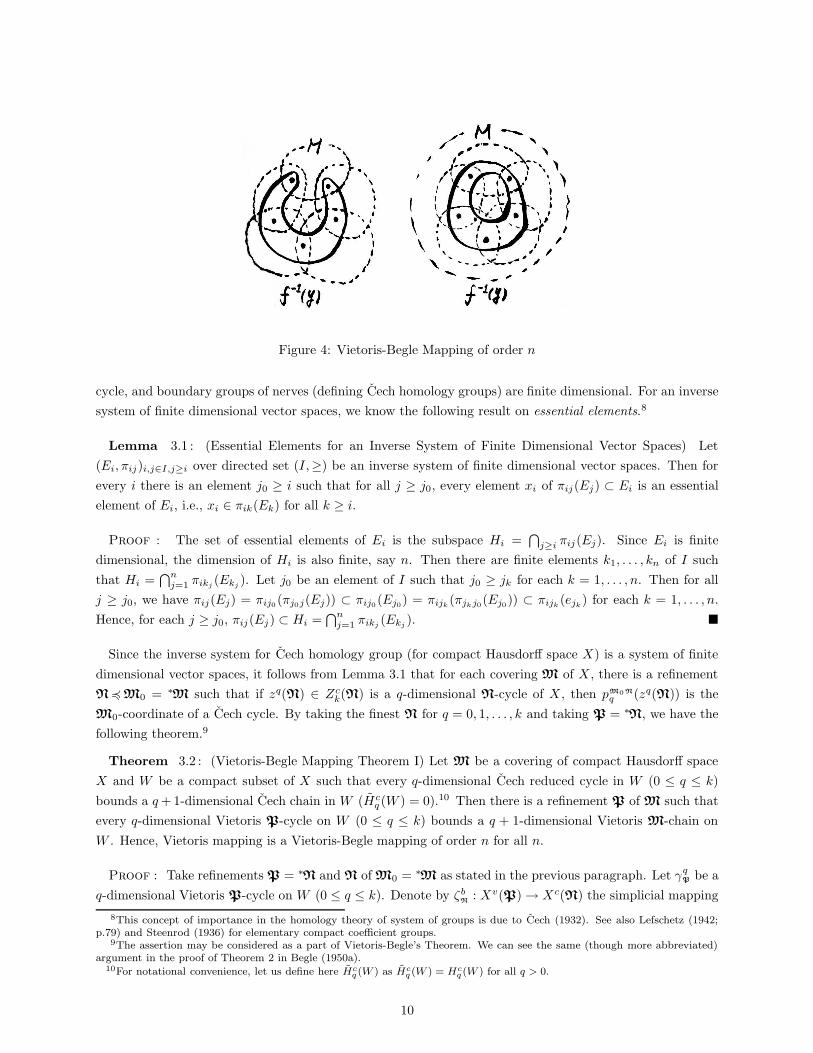
Figure 4: Vietoris-Begle Mapping of order n

cycle, and boundary groups of nerves (defining Cech homology groups) are finite dimensional. For an inverse

system of finite dimensional vector spaces, we know the following result on essential elements.8

Lemma 3.1 : (Essential Elements for an Inverse System of Finite Dimensional Vector Spaces) Let

(Ei, πij)i,j∈I,j≥i over directed set (I,≥) be an inverse system of finite dimensional vector spaces. Then for

every i there is an element j0 ≥ i such that for all j ≥ j0, every element xi of πij(Ej) ⊂ Ei is an essential

element of Ei, i.e., xi ∈ πik(Ek) for all k ≥ i.

Proof : The set of essential elements of Ei is the subspace Hi =⋂

j≥i πij(Ej). Since Ei is finite

dimensional, the dimension of Hi is also finite, say n. Then there are finite elements k1, . . . , kn of I such

that Hi =⋂n

j=1 πikj(Ekj

). Let j0 be an element of I such that j0 ≥ jk for each k = 1, . . . , n. Then for all

j ≥ j0, we have πij(Ej) = πij0 (πj0j(Ej)) ⊂ πij0 (Ej0) = πijk(πjkj0(Ej0)) ⊂ πijk

(ejk) for each k = 1, . . . , n.

Hence, for each j ≥ j0, πij(Ej) ⊂ Hi =⋂n

j=1 πikj(Ekj

). �

Since the inverse system for Cech homology group (for compact Hausdorff space X) is a system of finite

dimensional vector spaces, it follows from Lemma 3.1 that for each covering M of X , there is a refinement

N4 M0 = ∗M such that if zq(N) ∈ Zck(N) is a q-dimensional N-cycle of X , then pM0N

q (zq(N)) is the

M0-coordinate of a Cech cycle. By taking the finest N for q = 0, 1, . . . , k and taking P = ∗N, we have the

following theorem.9

Theorem 3.2 : (Vietoris-Begle Mapping Theorem I) Let M be a covering of compact Hausdorff space

X and W be a compact subset of X such that every q-dimensional Cech reduced cycle in W (0 ≤ q ≤ k)

bounds a q+ 1-dimensional Cech chain in W (Hcq (W ) = 0).10 Then there is a refinement P of M such that

every q-dimensional Vietoris P-cycle on W (0 ≤ q ≤ k) bounds a q + 1-dimensional Vietoris M-chain on

W . Hence, Vietoris mapping is a Vietoris-Begle mapping of order n for all n.

Proof : Take refinements P = ∗N and N of M0 = ∗M as stated in the previous paragraph. Let γqP be a

q-dimensional Vietoris P-cycle on W (0 ≤ q ≤ k). Denote by ζbN

: Xv(P)→ Xc(N) the simplicial mapping

8This concept of importance in the homology theory of system of groups is due to Cech (1932). See also Lefschetz (1942;p.79) and Steenrod (1936) for elementary compact coefficient groups.

9The assertion may be considered as a part of Vietoris-Begle’s Theorem. We can see the same (though more abbreviated)argument in the proof of Theorem 2 in Begle (1950a).

10For notational convenience, let us define here Hcq (W ) as Hc

q (W ) = Hcq (W ) for all q > 0.

10

Figure 5: Cycles on Acyclic Set W

defined in the proof of Theorem 2.3. Then ζbNq(γ

qP) is a q-dimensional Cech N-cycle (0 ≤ q ≤ k). By definition

of N, pM0N

q ζbN

(γqP) is the M0-coordinate of a Cech cycle, zq, onW . Since Hc

q (W ) = 0, this Cech cycle bounds

so that pM0N

q ζbN

(γqP) ∼ 0 on Cc

q (M0). It follows that ϕbMpM0N

q ζbN

(γqP) ∼ 0 on W v(M) = Xv(M)∩W , where

ϕbM

is the simplicial mapping defined in the proof of Theorem 2.3 and Xv(M)∩W denotes the subcomplex of

Vietoris M-simplexes on W . Hence, the first assertion of this theorem follows if we see ϕbMpM0N

q ζbN

(γqP) ∼ γq

P

on Xv(M)∩W . We can see it, however, by repeating completely the same argument with (2-2) in the proof

of Theorem 2.3. The second assertion follows immediately from the first if we set W = f−1(y) for Vietoris

mapping f : X → Y and point y ∈ Y . �

Locally Connected Spaces

Besides the Vietoris-Begle mapping, there is another important concept for fixed point arguments under

the Cech type homology, the local connectedness. In the Cech type homology theory, the family of open

coverings, Cover(X), on space X is used in describing two fundamental features of topological arguments: (i)

the measure of connectivity (represented by the intersection property among open sets), and (ii) the measure

of convergence or approximation (as a net of refinements of coverings). All analytic concepts are changed

into algabraic ones through above two channels. In the following, it is especially important to notice about

the second feature, so that each covering M ∈ Cover(X) is used as a sort of metric or a norm, and Cover(X)

is used as if it were the uniformity in describing the total convergence properties for space X . To emphasize

that we are choosing a covering or a refinement for the second purpose, we call it norm covering or norm

refinement instead of saying a covering or refinement.

The local connectedness is defined as a purely homological notion to generalize the concept of absolute

neighborhood retracts frequently used under the framework of metrizable spaces. Let us consider a compact

Hausdorff space Y and M ∈ Cover(Y ). A realization of simplicial complex K in Y v(M) is a chain map τ .

Partial realization τ ′ of K is a chain map defined on a subcomplex L of K such that Vert(L) = Vert(K).

For a norm covering N ∈ Cover(X) and realization τ of K, write norm(τ) ≤ N if for each simplex σ of K,

there is a set N ∈N which contains the underlying space |τσ| of the chain τσ.11

11For a value under a homomorphism, parenthesis are abbreviated as τσ = τ(σ). Note also that the underlying space of chainτσ is the underlying space of the corresponding complex defined by all simplexes of τσ (appeared with non-zero coordinates inthe formal summation).

11

Definition 3.3 : (Locally Connected Space) Topological space X is said to be locally connected (ab-

breviated by lc) if for each norm covering E ∈ Cover(X) there is a norm refinement J 4E satisfying the

following condition: for each covering M, there is a refinement N such that every partial realization τ ′ of

finite complex K into Xv(N) with norm(τ ′) ≤ J may be extended to a realization τ into Xv(M) with

norm(τ) ≤ E.

It is clear from the definition that if X is lc, then X × X is also lc. If X is a compact Hausdorff and lc,

then every closed subset of X is also lc. Moreover, compact Hausdorff lc spaces has the following strong

properties.

Theorem 3.4 : (Begle 1950b) If X is compact Hausdorff lc space, following (a) (b) (c) hold.

(a) There is a covering N0 of X such that if z is a Vietoris cycle such that z(N) ∼ 0 on Xv(N) for some

N4 N0, then z ∼ 0.

(b) The homology groups of X are isomorphic to the corresponding groups of a finite complex.

(c) Each covering M of X has a normal refinement M′, i.e., a refinement such that for each cycle zM′ on

Xv(M′) ⊂ Xv(M), there is a Vietoris cycle z such that z(M) = zM′ .

Proofs are not so difficult. See Begle (1950b).

4 Nikaido’s Analogue of Sperner’s Lemma

In this section we see the important second half of the Vietoris-Begle mapping theorem, (2) if f : X → Y

is a Vietoris-Begle mapping of order n, there are isomorphisms between Hvq (X) and Hv

q (Y ) (0 ≤ q ≤ n).

For this proof, we need the concept of barycentric subdivision under the framework of Vietoris complexes.

After the proof of Vietoris-Begle mapping theorem, we also see an extension of Sperner’s lemma which was

originally given by Nikaido (1959) as the first application.

Vietoris-Begle Barycentric Subdivision

Let Y be a compact Hausdorff topological space. Consider coverings N ∈ Cover(Y ) and R ∈ Cover(Y )

of Y . In the following, for Vietoris M-chain c(M) ∈ Cvq (M), let us denote by K(c(M)) the complex

of all simplexes appeared with positive coefficients in c(M) and by diam |c(M)| ≤ N the fact that there

is an element N ∈ N in which all vertices of K(c(M)) belong. Moreover, for each q-dimensional chain

cq ∈ Cvq (N) and y ∈ Y , we denote by y ∗ c the (q+ 1)-dimensional {Y }-chain defined as the extension of the

operation y ∗ 〈a0 · · · ak〉 = 〈ya0 · · · ak〉 for each oriented k-dimensional simplex 〈a0 · · ·ak〉.12 RN-barycentric

subdivision of k-dimensional Vietoris R-simplex σk ∈ Xv(R) is chain map Sdq : Cvq (R)→ Cv

q (N), satisfying

the following conditions.

(SD1) For each 0-dimensional simplex y0 of K(σk), Sd0(y0) = y0.

(SD2) For each q-dimensional simplex 〈y0 · · · yq〉 (0 < q ≤ k) in K(σk), there exists y ∈ Y such that y∗

Sdq−1(〈y0 · · · yi · · · yq〉) ∈ Cvq (N) for each i and Sdq(〈y0 · · · yq〉) =

∑qi=0(−1)iy∗Sdq−1(〈y0 · · · yi · · · yq〉).

(SD3) diam |Sdkσk| ≤N.

12Note that in the above {Y } ∈ Cover(Y ) is taken as a covering of Y .

12

Note that as long as the existence of y for each q-dimensional R-simplex 〈y0 · · · yq〉 stated in (SD2) is assured,

condition (SD1) and (SD2) may be considered as a process to construct Sdq , q = 0, 1, · · ·. By mathematical

induction, we can verify for each q > 0 that ∂qSdq(〈y0 · · · yq〉) = Sdq−1∂q(〈y0 · · · yq〉), so that Sdq constructed

is indeed a chain map.

Let us consider n-skeleton Y vn (R) ⊂ Y v(R) of Y v(R), the subcomplex of all k-dimensional (0 ≤ k ≤ n)

Vietoris R-simplexes on Y . An n-dimensional RN-barycentric subdivision of Y is a chain map {SdRN

q :

Cvq (Y v

n (R)) → Cvq (N)} such that for each k-dimensional simplex σk (0 ≤ k ≤ n), the restriction of {SdRN

q }

on the chain of subcomplex of Y vn (R) defined by σk is an RN-barycentric subdivision of σk.

Next, assume that there is a continuous onto map f on compact Hausdorff space X to Y . For each pair

of coverings M ∈ Cover(X) and N ∈ Cover(Y ) such that M 4{f−1(N)|N ∈ N}, f induces simplicial map

Xv(M) 3 a0 · · · ak 7→ f(a0) · · · f(ak) ∈ Y v(N) so that chain map {fq : Cvq (M) → Cv

q (N)}. Then as we

can see in the next theorem, if f is Vietoris-Begle mapping of order n, there is a chain map τ = {τq} on

(n+1)-skeleton of Y v(R) to X(M) such that {fq ◦τq} is an n+1-dimensional (RN)-barycentric subdivision

of Y . Moreover, given M, such refinement R may be taken arbitrarily small and corresponding τ ’s may be

defined as (Vietoris homologically) unique.

Theorem 4.1 : Let X and Y be compact Hausdorff spaces and let f : X → Y be a Vietoris-Begle

mapping of order n. For each M ∈ Cover(X) and N ∈ Cover(Y ) such that M 4{f−1(N)|N ∈ N}, there

exist a cover R = R(M,N) ∈ Cover(Y ) and a chain map τ = {τq} on (n+1)-skeleton of Y v(R) to Xv(M)

such that chain map {fq ◦ τq} is an n-dimensional (RN)-barycentric subdivision of Y . Moreover, for any

S ∈ Cover(Y ), there are R′ and τ ′ satisfying the same condition with R and τ such that R′4S and

τ ′q(zq) ∼ τq(zq) in Cv

q (M) for all zq ∈ Zvq (R′).

Above theorem shows an essential feature of the Vietoris-Begle mapping and plays crucial roles in the

proof of the Vietoris-Begle mapping theorem. Before proving it, I introduce one technical lemma. In Lemma

2.2, we have seen one of the simplest kind of prismatical relation that may be utilized to show the equivalence

between two cycles. There exists another convenient (though a little bit more complicated) method in forming

prisms. Denote by {0, 1, I} the one dimensional abstract complex formed by two 0-dimensional simplices 0

and 1 together with 1-dimensional simplex I whose boundaries are 0 and 1 under relation ∂1(I) = 1 − 0.

For simplicial complex K, the product complex of K and {0, 1, I} denoted by K × {0, 1, I} is the family of

simplexes of the form σ×0, σ×1, and σ×I , where σ runs through all simplexes in K. Boundary relations on

K×{0, 1, I} are defined as ∂(σ×0) = (∂σ)×0, ∂(σ×1) = (∂σ)×1, and ∂(σ×I) = (∂σ)×I+(σ×1)−(σ×0).

(See Figure 6.) It should be noted that K × {0, 1, I} is no longer a simplicial complex. The subcomplex

of K × {0, 1, I} constructed by all simplexes of the form σ × 0 may clearly be identified with K and is

called the base of K × {0, 1, I}. There also exists an isomorphism between K and the subcomplex of all

simplexes of the form σ × 1, which is called the top of K × {0, 1, I}. Then for each cycle z on K, we have

∂(z × I) = (z × 1) − (z × 0), immediately, so that z × 1 ∼ z × 0 in K × {0, 1, I}. Therefore, as before

(Lemma 2.2) if there exists a chain mapping θ on K × {0, 1, I} to a certain simplicial complex L, we have

the following.

Lemma 4.2 : Assume that there is a chain mapping θ on K ×{0, 1, I} to simplicial complex L. For two

images θq+1(zq × 0) and θq+1(z

q × 1) in the q-th chain group Cq(L) of q-cycle zq ∈ Cq(K) (through the

induced homomorphism θq+1 : Cq+1(K × {0, 1, I})→ Cq(L)), we have θq+1(zq × 0) ∼ θq+1(z

q × 1) on L.

13

Figure 6: Prism K × {0, 1, I}

Proof of Theorem 4.1 : We shall use four steps. Step 1 is devoted to prepare for basic tools. In Step

2, we construct R. Step 3 is used to define τ . Step 4 is assigned for constructions of R′ and τ ′.

(Step1) By the definition of Vietoris-Begle mapping, there is a covering P(M, y) for each y ∈ Y

and M. Consider closed (compact) subset X \ St(f−1(y); ∗P(M, y)). Then the image under f of X \

St(f−1(y); ∗P(M, y)) is also closed (compact) subset of the normal space Y disjointed from {y}. Given

N ∈ Cover(Y ), chose Q(M,N, y) 3 y as an element of ∗N and Q(M,N) as a finite subcovering of the cov-

ering {Q(M,N, y)|y ∈ Y }. Then covering Q(M,N) satisfies that if B is a subset of Y such that B ⊂ Q for

some Q ∈Q(M,N), there is a point y ∈ Y such that St(y; ∗N) ⊃ B and St(f−1(y); ∗P(M, y)) ⊃ f−1(B).

In this proof we call this y the corresponding point of Y to B and use it as if it were the barycenter of points

in B.

(Step 2) Hence, for each M ∈ Cover(X) and N ∈ Cover(Y ), Q(M,N) ∈ Cover(Y ) satisfies that for every

q-dimensional Q(M,N)-simplex 〈y0 · · · yq〉, (0 ≤ q ≤ n), there is a point y ∈ Y such that y ∗ 〈y0 · · · yq〉

is a ∗N-simplex and St(f−1(y); ∗P(M, y)) ⊃ f−1({y0, . . . , yq}). This suggests the possibility to obtain a

sequence of refinements M1 4 · · ·4Mn+1 = M together with refinements N0 4 · · ·4Nn+1 = N such that

Mk 4{f−1(N)|N ∈ Nk} for each k = 1, . . . , n + 1, and for each q-dimensional Nq-simplex (q = 0, . . . , n)

〈y0 · · · yq〉, there exists y ∈ Y such that y ∗ 〈y0 · · · yq〉 is a ∗Nq+1-simplex and St(f−1(y); ∗P(Mq+1, y)) ⊃

f−1({y0, . . . , yq}). (As we see in the next step, under the definition of barycentric subdivision (SD1)–(SD3),

this property shows that for each n + 1-dimensional N0-simplex we are possible to define an N0Nn+1-

barycentric subdivision.) Indeed, given Nn+1 = N and Mn+1 = M, set Nn = Q(Mn+1,∗Nn+1) 4 ∗∗Nn+1.

Note that with Q(Mn+1,∗Nn+1) associates finite yn+1,i’s such that Q(Mn+1,

∗Nn+1) consists of Q(Mn+1,∗Nn+1, yn+1,i)’s. Let Mn be a common refinement of coverings ∗P(Mn+1, yn+1,i)’s and {f−1(N)|N ∈Nn}.

Set Nn−1 = Q(Mn,∗Nn). Repeat the process until we obtain N0. Define R as R = R(M,N) = N0.

(Step 3) Let us define τq (0 ≤ q ≤ n) on chains of Y v(R) = Y v(N0) to Xv(M). Consider a 0-

dimensional Vietoris R-simplex, σ0, of Y v(R). σ0 may be identified with a point y0 in Y . Define τ(σ0)

as 0-dimensional Vietoris M0-simplex ξ0 of Xv(M0) which may be identified with an arbitrary point

x0 ∈ f−1(y0) ⊂ X . Then we have f0 ◦ τ0(σ0) = σ0 = Sd0(σ0), so that we obtain τ0 by linearly extending

it. Next, consider k-dimensional Vietoris R-simplex, σk, of Y v(R) (0 < k ≤ n+ 1). Suppose that for each

(k − 1)-dimensional R-simplex σk−1, τk−1(σk−1) is already defined and satisfies that fk−1 ◦ τk−1(σ

k−1) is a

R ∗Nk−1-barycentric subdivision of σk−1 together with the relation of chain map, ∂k−2 ◦ τk−1 = τk−2 ◦∂k−1,

14

where τk−2 for k = 1 is defined to be 0-map. In the following, we see that we may define τk(σk) so

as to satisfy that ∂k−1 ◦ τk = τk−1 ◦ ∂k and fkτkσk is a R ∗Nk-barycentric subdivision of σk for each

k-dimensional Vietoris R-simplex σk. Then by the mathematical induction, we may extend the defini-

tion of τk until it is finally defined on all of the (n + 1)-skeleton of Y (R). Since ∂kσk is an R-chain,

τk−1∂kσk is already defined and is a Mk-cycle since ∂k−1τk−1∂kσ

k = τk−2∂k−1∂kσk = 0. By assump-

tion fk−1τk−1∂kσk = fk−1τk−1

∑ki=0(−1)iσk−1

i =∑k

i=0(−1)ifk−1τk−1σk−1i belongs to Cv

k−1(∗∗Nk−1), where

σk−1i ’s are k + 1 (k − 1)-dimensional face of σk, and fk−1τk−1σ

k−1i is a R ∗Nk−1-barycentric subdivision of

σk−1i for each i. It follows that all vertices of the ∗∗Nk−1-chain, fk−1τk−1∂kσ

k = fk−1τk−1

∑ki=0(−1)iσk

i =∑k

i=0(−1)kfk−1τk−1σki , belongs to St(R0;

∗∗Nk−1) ⊂ St(∗∗Nk−1;∗∗Nk−1) for an R0 ∈ R having all vertices

of σk as its elements and ∗∗Nk−1 ∈ ∗∗Nk−1 such that R0 ⊂ ∗∗Nk−1. Since there exists ∗Nk−1 ∈ ∗Nk−1 such

that St(∗∗Nk−1;∗∗Nk−1) ⊂

∗Nk−1, we have diam |fk−1τk−1∂kσk| ≤ ∗Nk−1. Then Nk−1 = Q(Mk,

∗Nk)

implies that there is corresponding point y = yk,i ∈ Y , Q(Mk,∗Nk, yk,i) ∈Q(Mk,

∗Nk), to |fk−1τk−1∂kσk|

satisfying the following two relations.13

St(y; ∗∗Nk) ⊃ |fk−1τk−1∂kσk|(6)

St(f−1(y); ∗P(Mk, y)) ⊃ f−1(|fk−1τk−1∂kσ

k|) ⊃ |τk−1∂kσk|(7)

Denote by zk−1 the cycle τk−1∂kσk ∈ Zv

k−1(Mk−1) and let x1, . . . , x` be vertices of K(zk−1). Note that by

(7), there are finite x′1, . . . , x′` ∈ f

−1(y) and ∗P1, . . . ,∗P` ∈ ∗P(Mk, y) such that x′1 ∈

∗P1, . . . , x′` ∈

∗P` and

x1 ∈ ∗P1, . . . , x` ∈ ∗P`. By defining mapping µ on Vert(K(zk−1) × {0, 1}) to X as µ(xi, 0) = xi for each

vertex (xi, 0) in the base of K(zk−1)×{0, 1} and µ(xi, 1) = x′i for each vertex (xi, 1) in the top of K(zk−1)×

{0, 1}. It is easy to check that µ is a simplicial map. Indeed, if ((a0, 0), . . . , (ai, 0), (ai, 1), . . . , (am, 1))

is a simplex in K(zk−1) × {0, 1}, then ((a0, 0), . . . , (am, 1)) is a simplex in K(zk−1), so that there exists

element Mk−1 ∈ Mk−1 such that a0, . . . , am ∈ Mk−1. Since ai is equal to some xj , and both (xj , 0)

and (xj , 1) are in ∗Pj , all vertices in (a0, . . . , ai, µ(ai, 1), . . . , µ(am, 1)) belong to St(Mk−1,∗P(Mk, y)). By

considering the fact that Mk−1 4 ∗P(Mk, y), they belong to an element of P(Mk, y), so that µ maps

K(zk−1) simplicially to Xv(P(Mk, y)). Let us use µ to define τk(σk) as follows: Set ξk1 = µ(Φk(zk−1)),

where Φk is the prismatic chain homotopy defined in equations (1)–(3). By (3), we have ∂k(µΦkzk−1) =

µ(zk−1 × 1)− µ(zk−1 × 0) = µ(zk−1 × 1)− zk−1. Since µ(zk−1 × 1) is a cycle on Xv(P(Mk, y)) ∩ f−1(y),

there is a chain ξk2 on Xv(P(Mk, y))∩f

−1(y) such that ∂kξk2 = µ(zk−1×1). Then if we set τk(σk) = ξk

2 −ξk1 ,

we have ∂kτkσk = zk−1 = τk−1∂k−1σ

k , so that τk satisfies the condition for chain map. Moreover, since

fk(τkσk) = fk(ξk

2 − ξk1 ) = fk(ξk

2 )− fk(µ(Φk(zk−1))), we may also rewrite it as fk(ξk2 ) − µ(Φk(fk−1z

k−1)) =

fk(ξk2 )− µ(Φk(fk−1τk−1∂kσ

k)) = fk(ξk2 ) − µ(Φk(Sdk−1∂kσ

k)), where Φ is the prismatic chain homotopy on

complex K(fk−1(zk−1)) to K(fk−1(z

k−1)) × {0, 1} and µ is defined on K(fk−1(zk−1)) in exactly the same

way as µ, i.e., µ(f(xi), 0) = f(xi) and µ(f(xi), 1) = f(x′i) = y. Since St(y; ∗∗Nk) ⊃ |fk−1τk−1∂kσk|, µ is

a simplicial map on K(fk−1(zk−1)) × {0, 1} to Y v(∗Nk). Moreover, fk(τkσ

k) is clearly the join of y with

Sdk−1 ∂kσk with diam | Sdk σ

k | ≤ ∗Nk.

(Step 4) Take M′1 4 · · ·4 M′

n+1 and N′0 4 · · ·4N′

n+1 in the same way as M1 4 · · · 4 Mn+1 and

N0 4 · · ·4Nn+1 except for the process to define Nk (k ≤ n). Let us define N′k as a common refinement

of Q(M′k+1,

∗N′k+1),

∗Nk, and S for each k ≤ n. Define R′ as N′0 and τ ′k (0 ≤ k ≤ n + 1) in exactly

the same way as τk. We now check for each R′-cycle zn, τn(zn) = τ ′n(zn). For this purpose, it is sufficient

by Lemma 4.2 to show mapping θ to Xv(M) such that for each σk × 0, θ(σk × 0) = τk(σk), and for each

σk × 1, θ(σk × 1) = τ ′k(σk), (0 ≤ k ≤ n), may be extended as a chain mapping on K(zn)× {0, 1, I}. On the

13For Vietoris P-chain c, |c| denotes the set of all vertices of simplexes appeared in c with positive coefficients.

15

base and top of K(zn) × {0, 1, I}, θ clearly defines chain maps since we have ∂k(θkσk × 0) = ∂k(τk(σk)) =

τk−1(∂kσk) = θk−1(∂kσ

k × 0) and ∂k(θkσk × 1) = ∂k(τ ′k(σk)) = τ ′k−1(∂kσ

k) = θk−1(∂kσk × 1).

Let us consider a 0-dimensional simplex σ0 in K(zn) and σ0 × I ∈ K(zn) × {0, 1, I}. By definition

(in Step 3) f0τ0σ0 = f0τ

′0σ

0 = σ0 and both τ0(σ0) and τ ′0(σ

0) are points in f−1(σ0) = f−1(|f0τ0σ0|) =

f−1(|f0τ ′0σ0|) ⊃ |τ0σ0| ∪ |τ ′0σ

0|. Then it is automatically satisfied that there exists y (y = σ0) such that

St(y; N1) ⊃ |σ0| and

St(f−1(y); ∗P(M1, y)) ⊃ f−1(σ0).

Note that θ∂(σ0 × I) = τ(σ0) − τ ′(σ0). Hence, we have St(f−1(y); ∗P) ⊃ |θ∂(σ0 × I)| (Figure 7). Let

Figure 7: y and θ∂(σk × I)

us consider simplicial complex K = K(τ(σ0) − τ ′(σ0)) and mapping ω : Vert(K × {0, 1}) to X such that

ω(a, 0) = a and ω(a, 1) = ya, where ya is an element of f−1(y) satisfying {a, ya} ⊂ ∗P for some ∗P ∈ ∗P.

Such ya exists since St(f−1(y); ∗P) ⊃ |θ∂(σ0 × I)|. Then ω is a simplicial map on K ×{0, 1} to Xv(P). As

before, let us define ξ11 as ξ11 = ω(Φ(τ0σ0− τ ′0σ

0)), where Φ denotes the prismatic chain homotopy. Note that

∂ξ11 = ω((τ0σ0− τ ′0σ

0)× 1)− (τ0σ0− τ ′0σ

0). Now ω((τ0σ0− τ ′0σ

0)× 1) is a 0-cycle (by the previous equation)

on Xv(P)∩ f−1(y), there is a 1-chain ξ12 on Xv(M1)∩ f−1(y) such that ∂ξ12 = ω((τ0σ0− τ ′0σ

0)× 1). Define

θ(σ0× I) to be ξ12− ξ11 . Then θ satisfies the condition of chain map ∂θ = θ∂ for σ0× I for each 0-dimensional

σ0. Clearly, f |ξ12 − ξ11 | is the join of y and σ0 = y, so that diam f |ξ12 − ξ

11 | ≤

∗N1

Next assume that θ(σm × I) is defined for each m ≤ k in such a way that ∂θ = ∂θ, θ(σm × I) ∈Mm+1,

and diam f |θ(σm × I)| ≤ ∗Nm+1. Let σk be a k-dimensional simplex of K(zn). Then θ(∂(σk × I)) is

already defined. Since θ(∂(σk × I)) = θ((∂σk) × I) + θ(σk × 1) − θ(σk × 0), we have f |θ(∂(σk × I))| ⊂

f |θ(∂σk)| ∪ f |τk(σk)| ∪ f |τ ′kσk|. By considering facts, diam f |τk(σk)| ≤ ∗Nk and diam f |τ ′k(σk)| ≤ ∗N′

k 4 ∗N,

we have St(R′; Nk) contains f |τk(σk)| and f |τ ′k(σk)|, where R′ denotes an element of R′ to which all

vertices of σk belong. It is also true by assumption that for each (k − 1)-dimensional face σk−1 of σk,

diam f |θ(σk−1 × I)| ≤ ∗Nk, so that we have diam f |θ∂(σk × I)| ≤Nk = Q(Mk+1,∗Nk+1). Hence, we have

a point y such that Q(Mk+1,∗Nk+1, y) ∈Q(Mk+1,

∗Nk+1),

St(y; ∗Nk+1) ⊃ f |θ∂(σk × I)| and

16

St(f−1(y); ∗P(Mk+1, y)) ⊃ f−1f |θ∂(σk × I)|.

Hence, we have St(f−1(y); ∗P(Mk+1, y)) ⊃ |θ∂(σk × I)|. (See Figure 7.) Consider again simplicial complex

K = K(θ∂(σk × I)) and mapping ω : Vert(K × I) to X , we may define θ(σk × I) in exactly the same way as

before until k = n in such a way that ∂θ(σk × I) = θ∂(σk × I), θ(σk × I) ∈Mk+1, and diam f |θ(σk × I)| ≤∗Nk+1. �

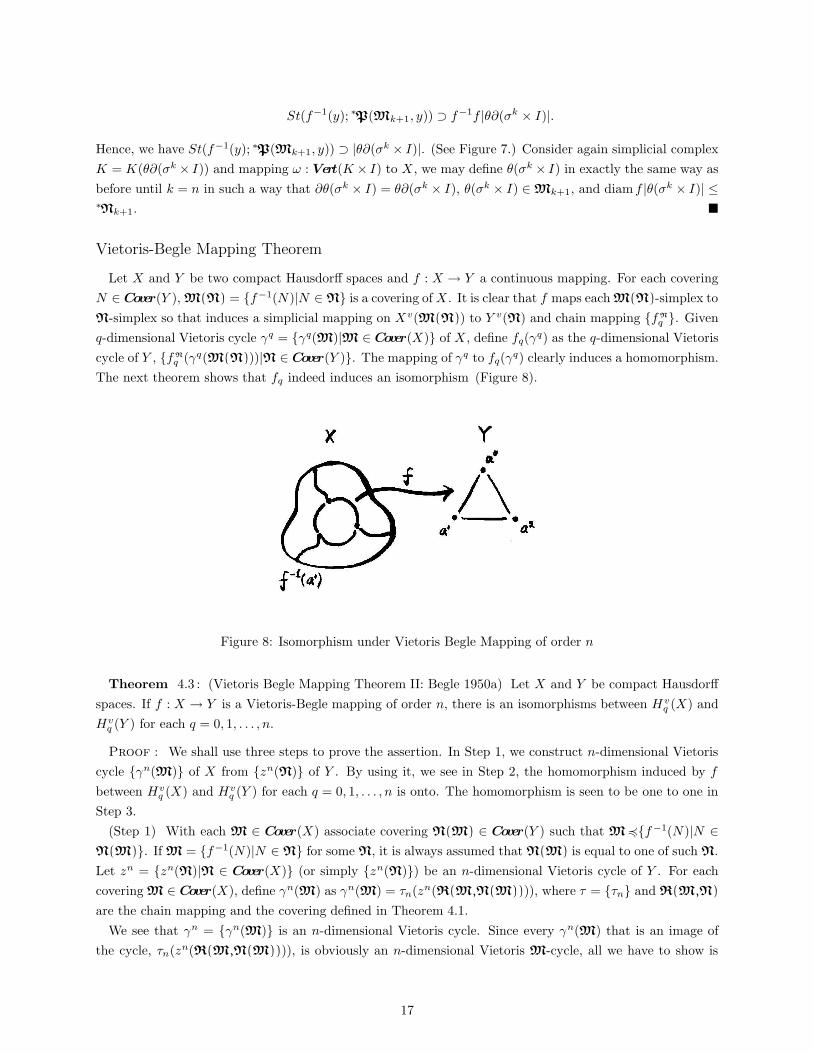
Vietoris-Begle Mapping Theorem

Let X and Y be two compact Hausdorff spaces and f : X → Y a continuous mapping. For each covering

N ∈ Cover(Y ), M(N) = {f−1(N)|N ∈N} is a covering ofX . It is clear that f maps each M(N)-simplex to

N-simplex so that induces a simplicial mapping on Xv(M(N)) to Y v(N) and chain mapping {fN

q }. Given

q-dimensional Vietoris cycle γq = {γq(M)|M ∈ Cover(X)} of X , define fq(γq) as the q-dimensional Vietoris

cycle of Y , {fN

q (γq(M(N)))|N ∈ Cover(Y )}. The mapping of γq to fq(γq) clearly induces a homomorphism.

The next theorem shows that fq indeed induces an isomorphism (Figure 8).

Figure 8: Isomorphism under Vietoris Begle Mapping of order n

Theorem 4.3 : (Vietoris Begle Mapping Theorem II: Begle 1950a) Let X and Y be compact Hausdorff

spaces. If f : X → Y is a Vietoris-Begle mapping of order n, there is an isomorphisms between Hvq (X) and

Hvq (Y ) for each q = 0, 1, . . . , n.

Proof : We shall use three steps to prove the assertion. In Step 1, we construct n-dimensional Vietoris

cycle {γn(M)} of X from {zn(N)} of Y . By using it, we see in Step 2, the homomorphism induced by f

between Hvq (X) and Hv

q (Y ) for each q = 0, 1, . . . , n is onto. The homomorphism is seen to be one to one in

Step 3.

(Step 1) With each M ∈ Cover(X) associate covering N(M) ∈ Cover(Y ) such that M 4{f−1(N)|N ∈

N(M)}. If M = {f−1(N)|N ∈N} for some N, it is always assumed that N(M) is equal to one of such N.

Let zn = {zn(N)|N ∈ Cover(X)} (or simply {zn(N)}) be an n-dimensional Vietoris cycle of Y . For each

covering M ∈ Cover(X), define γn(M) as γn(M) = τn(zn(R(M,N(M)))), where τ = {τn} and R(M,N)

are the chain mapping and the covering defined in Theorem 4.1.

We see that γn = {γn(M)} is an n-dimensional Vietoris cycle. Since every γn(M) that is an image of

the cycle, τn(zn(R(M,N(M)))), is obviously an n-dimensional Vietoris M-cycle, all we have to show is

17

γn(M) ∼ hMM''

n (γn(M'')) for each pair M''4 M. That is,

τn(zn(R(M,N(M)))) ∼ hMM''

n (τ ′′n (zn(R(M'', N(M'')))))

for each M''4 M, where τ ′′ is the chain mapping associated with R(M'',N(M'')). For a while, de-

note R(M'',N(M'')) by R'' and R(M,N(M)) by R. If we omit inclusion map hn, we have to show

τn(zn(R)) ∼ τ ′′n (zn(R'')).

In Step 4 of the proof of second assertion in Theorem 4.1, we may chose

M′1 4 · · ·4 M′

n+1 and N′0 4 · · ·4 N′

n+1

as common refinements not only of serieses {Mk} and {Nk} constructing τ (in Step 3) for M and N but

also of another streams {M''k} and {N''k} combined with chain map τ ′′ for M'' and N'' satisfying the same

condition with M and N. Since the construction of τ ′ is independent of τ and τ ′′, by repeating the same

argument (to construct θ′ instead of θ), we can see τ ′n(zn) ∼ τn(zn) and τ ′n(zn) ∼ τ ′′n (zn) in Cvn(M) for all

zn ∈ Zvn(R').

That is, there exists common refinement R' of R = R(M,N(M)) and R'' = R(M'',N(M'')) together

with chain map τ ′ such that τ ′(zn(R')) ∼ τ(zn(R')) and τ ′(zn(R')) ∼ τ ′′(zn(R')), where τ and τ ′′ are

the chain map associated respectively with R and R''. Hence we have τ(zn(R')) ∼ τ ′′(zn(R')). Since

zn is a Vietoris cycle, we know hRR'

n (zn(R')) ∼ zn(R) and hR''R'

n (zn(R')) ∼ zn(R''), so that we have

τ(zn(R)) ∼ τ ′′(zn(R'')).

(Step 2) We see that f induces an onto mapping. Let zn be an n-dimensional Vietoris cycle of X and

γn = {τn(zn(R(M,N(M))))} the n-dimensional Vietoris cycle of Y corresponding to zn. Let us verify

that fq(γn) ∼ zn. Given N ∈ Cover(Y ), let M be the covering {f−1(N)|N ∈ N}. Then γn(M) =

τ(zn(R)), where R = R(M,N(M)). It follows that the N-th coordinate of fn(γn), fN

n (γn(M)), is equal

to fN

n τnzn(R(M,N(M))). Note that N(M) may not equal to N. Since fN

n τnzn(R(M,N(M))) is an

(RN(M))-barycentric subdivision of zn(R(M,N(M))), zn(R) ∼ Sdn zn(R) = fN

n (τnzn(R(M,N(M))))

= fN

n (γn(M)) on Y v(N) (as well as on Y v(N(M))). Moreover, since zn is a Vietoris cycle, we have

zn(R) ∼ zn(N). It follows that zn(N) ∼ fN

n (γn(M)) on Y v(N).

(Step 3) Let us confirm the mapping induced by f is one to one. Since f clearly induces a homomorphism,

it is sufficient to show that fn(γn) ∼ 0 means γn ∼ 0 for each n-dimensional Vietoris cycle γn of X . Given

M ∈ Cover(X), chose N = N(M) and R = R(M,N(M)) as before. Let U = {f−1(R)|R ∈R}. Moreover

let us recall sequence {Mk} of refinements of M defined in the proof of Theorem 4.1 and V a common

refinement of U and all Mk’s.

Since γn is an n-dimensional Vietoris cycle, γn(V) ∼ γn(U) on Xv(U). Then we have fR

n γn(V) ∼

fR

n γn(U) on Y v(R). But if fn(γn) ∼ 0, R-th coordinate of fn(γn), fR

n γn(M(R)) = fR

n γn(U), satisfies

fR

n γn(U) ∼ 0 on Y v(R). Hence, we have fR

n (γn(V)) ∼ 0, so that τn(fR

n (γn(V))) ∼ 0, where τ = {τn}

is the chain map associated with R = R(M,N). Now it is possible to show τn(fR

n (γn(V))) ∼ γn(V) on

Xv(M). Indeed, let us consider K = K(γn(V)) and the product cell-complex K × {0, 1, I} together with

chain map θ defined on the base and top of K×{0, 1, I} to Xv(M) as θ(σk×0) = σk and θ(σk×1) = τkfkσk

for each simplex σk of K. We may extend θ as a chain map on K × {0, 1, I} in exactly the same way with

the process stated in the proof of Theorem 4.1. (In Step 4, substitute τkfkσk for τkσ

k and σk for τ ′k(σk).)

Then we have τn(fR

n (γn(V))) ∼ γn(V) on Xv(M), so that γn(V) ∼ 0 since τnfnγn(V) ∼ 0 on Xv(M).

Since γn is a Vietoris cycle, γn(V) ∼ γn(M). Thus γn(M) ∼ 0 on Xv(M), so γn ∼ 0. �

18

Analogue of Sperner’s Lemma

Nikaido (1959) treats a theorem which may be considered as an extension of Sperner’s lemma based

on Vietoris-Begle mapping theorem. Let X and Y be compact Hausdorff spaces. Suppose that Y may be

identified (under homeomorphism) with n-dimensional simplex 〈a0a1 · · · an〉 in Euclidean (n+1)-space Rn+1.

Moreover, assume that there is continuous onto function f : X → Y . For each k-dimensional face ai0 · · ·aik

of a0 · · ·an, denote by [ai0 · · · aik ] the set of all convex combination of points of {a0, . . . , ak}. In this section,

we call f−1([ai0 · · · aik ]) a k-face of X . For point x of X , there exists the smallest dimensional face ai0 · · ·aik

such that f(x) ∈ [ai0 · · · aik ], the carrier of f(x). We also call such f−1([ai0 · · · aik ]) the carrier of x (Figure

9).

Figure 9: Faces and Carriers

Let us consider a covering M ∈ Cover(X) of X and Vietoris M-complex Xv(M). Denote by K(Y ) the

simplicial complex K(〈a0a1 · · · an〉). Suppose that there exists a chain map τ = {τq} on chains of K(Y ) to

chains of Xv(M), τq : Cq(K(Y ))→ Cvq (M), satisfying the following two conditions:

(T1) τk(ai0 · · · aik ) ⊂ f−1([ai0 · · · aik ]) for any k-face ai0 · · ·aik of Y .

(T2) τ0(ai) is a single point for each vertex ai of Y .

We can always construct such τ when f is a Vietoris-Begle mapping. (The same process with the construction

of Vietoris-Begle barycentric subdivision in Theorem 4.1 may be utilized.) Operator τ may be considered

as a generalization of the usual barycentric subdivision. If X = Y and f is the identity mapping, it is clear

that chain map Sd satisfies conditions (T1) and (T2).

A vertex assignment v is a mapping on X = Vert(Xv(M)) to {a0, a1, . . . , an} = Vert(K(Y )) such that for

each x ∈ X , v(x) is a vertex of the carrier of f(x). Obviously, v is a simplicial mapping on Xv(M) to K(Y ),

so that induces a chain homomorphism which we also denoted by v or {vq}, vq : Cvq (M) → Cq(K(Y )).

Given vertex assignment v, we call n-dimensional simplex σn in Xv(M) regular if vn(σn) = 〈a0a1 · · · an〉

or vn(σn) = −〈a0a1 · · ·an〉. It is also convenient to define a sign ε(σm) of an m-simplex of Xv(M) for

each m = 0, 1, . . . , n, as ε(σm) = 1 if vm(σm) = 〈a0a1 · · · am〉, ε(σm) = −1 if vm(σm) = −〈a0a1 · · · am〉,

and ε(σm) = 0 otherwise. In the next lemma, we use J as an index set for all n-dimensional simplexes in

19

Xv(M).14

Lemma 4.4 : (Nikaido 1959: Sperner’s Lemma) Let τn(〈a0a1 · · ·an〉) =∑

j∈J αjσnj , where τ denotes

the chain map defined above. Then∑

j∈J αjε(σnj ) 6= 0. Especially, there exists at least one regular simplex

for an arbitrary vertex assignment.

Proof : Note that in the above expression, τn(〈a0a1 · · · an〉) =∑

j∈J αjσnj , the value of τn,

∑j∈J αjσ

nj ,

is a finite sum by definition of the chain map, so that αj = 0 except for finitely many j ∈ J . By condition

(T2), the lemma is clearly true for n = 0. In the following we show the lemma by using the mathematical

induction over n. Let K be an index set for all (n− 1)-dimensional simplexes in Xv(M). We call (n − 1)-

dimensional simplex σn−1 in Xv(M) regular if vq(σn−1) = 〈a1 · · · an〉 or vq(σ

n−1) = −〈a1 · · · an〉. Assume

that the lemma is true for n − 1, i.e., for f restricted on f−1([a1 · · ·an]) to K(〈a1 · · · an〉), τ restricted on

chains of K(〈a1 · · · an〉), and an arbitrary vertex assignment v on X to {a1 · · · an},

τn−1(〈a1 · · · an〉) =∑

k∈K

βkε(σn−1k ) 6= 0,

where the summation is taken over all k ∈ K for the sake of notational simplicity. (There is no problem since

ε(σn−1k ) = 0 for all σn−1

k /∈ Xv(M) ∩ f−1([a1 · · · an]) by the definition of ε.) For our purpose, it is sufficient

to show that ∑

j∈J

αjε(σnj ) =

∑

k∈K

βkε(σn−1k ).

(Step 1) First, let us see that

∑

j∈J

αjε(σnj ) =

∑

j∈J

αj

∑

k∈K

[〈σn−1k 〉 : 〈σn

j 〉]ε(σn−1k ),

where [ · : · ] denotes the incidence number. Indeed, when σnj is regular, there is one and only one regular

(n−1)-face σn−1k of σn

j . Let 〈σn−1k 〉 = 〈u1 · · ·un〉. If [〈σn−1

k 〉 : 〈σnj 〉] = 1, then by using a certain point u0 ∈ X ,

we may write 〈σnj 〉 = 〈u0u1 · · ·un〉. Hence, vn(σn

j ) = 〈v(u0)v(u1) · · · v(un)〉 = ±〈a0a1 · · ·an〉 if and only if

vn−1(σn−1k ) = 〈v(u1) · · · v(vn)〉 = ±〈a1 · · · an〉. Therefore, ε(σn

j ) = ε(σn−1k ). If [〈σn−1

k 〉 : 〈σnj 〉] = −1, then we

may write 〈σnj 〉 = −〈u0u1 · · ·un〉. Hence, vn(σn

j ) = −〈v(u0)v(u1) · · · v(un)〉 = ±〈a0a1 · · · an〉 if and only if

vn−1(σn−1k ) = 〈v(u1) · · · v(vn)〉 = ∓〈a1 · · ·an〉. Therefore, ε(σn

j ) = −ε(σn−1k ). In each cases, we have ε(σn

j ) =∑

k∈K [〈σn−1k 〉 : 〈σn

j 〉]ε(σn−1k ). When σn

j is not regular, we must show that∑

k∈K [〈σn−1k 〉 : 〈σn

j 〉]ε(σn−1k ) = 0

even if σnj has regular faces. Suppose that σn−1

i is a regular face of σnj and let 〈σn−1

i 〉 = 〈u1 · · ·un〉.

There is a point u0 of X such that Vert(σnj ) = {u0, u1, . . . , un}. Since σn

j is not regular, there is an m

such that v(u0) = v(um). Let σn−1k be the face of σn

j whose vertices are {u0, u1, . . . , un} \ {um}. Let

〈σn−1k 〉 = 〈w1 · · ·wn〉. Clearly, σn

j has exactly two regular faces, σn−1i and σn−1

k . Then, if [〈σn−1i 〉 : 〈σn

j 〉] = 1

and [〈σn−1k 〉 : 〈σn

j 〉] = ±1, we have 〈σnj 〉 = 〈u0u1 · · ·un〉 and 〈σn

j 〉 = ±〈umw1 · · ·wn〉. Since 〈u0u1 · · ·un〉 =

−〈umu1 · · ·um−1u0um+1 · · ·un〉, we have 〈umw1 · · ·wn〉 = ±〈u0u1 · · ·un〉 = ∓〈umu1 · · ·um−1u0um+1 · · ·un〉,

so that 〈v(w1)v(w2) · · · v(wn)〉 = ∓〈v(u1) · · · v(um−1)v(u0)v(um+1) · · · v(un)〉 = ∓〈v(u1)v(u2) · · · v(un)〉. It

follows that ε(σn−1k ) = ∓ε(σn−1

i ). In exactly the same way, if [〈σn−1i 〉 : 〈σn

j 〉] = −1 and [〈σn−1k 〉 : 〈σn

j 〉] = ±1,

we obtain that ε(σn−1k ) = ±ε(σn−1

i ). Therefore, we have [〈σn−1i 〉 : 〈σn

j 〉]ε(σn−1i ) + [〈σn−1

k 〉 : 〈σnj 〉]ε(σ

n−1k ) = 0

in all cases, so that∑

k∈K [〈σn−1k 〉 : 〈σn

j 〉]ε(σn−1k ) = 0.

(Step 2) Next, we see that

∑

j∈J

αj

∑

k∈K

[〈σn−1k 〉 : 〈σn

j 〉]ε(σn−1k ) =

∑

k∈K

βkε(σn−1k ).

14Recall that we treat only finite chains, so that in the formal summation all but a finite number of coefficients are 0.

20

Note that since τn(〈a0 · · · an〉) =∑

j∈J αjσnj , we have

∂n(τn(〈a0 · · · an〉)) = ∂n(∑

j∈J

αjσnj ) =

∑

j∈J

αj∂n(σnj ) =

∑

j∈J

αj

∑

k∈K

[〈σn−1k 〉 : 〈σn

j 〉]σn−1k .

Moreover, since ∂τ = τ∂, we also have

∂n(τn(〈a0 · · ·an〉)) = τn−1∂n(〈a0 · · · an〉) =

n∑

i=0

(−1)iτn−1(〈a0 · · · ai · · ·an〉),

where the circumflex accent denotes the omission of vertex ai. It follows that

∑

j∈J

αj

∑

k∈K

[〈σn−1k 〉 : 〈σn

j 〉]σn−1k =

n∑

i=0

(−1)iτn−1(〈a0 · · · ai · · · an〉).

Since τn−1(〈a0 · · · ai · · ·an〉) ⊂ f−1([a0, · · · , ai, · · · , an]) (Condition (T1)), by considering the fact that each

σn−1k appearing in the formal summation τn−1(〈a0 · · · ai · · ·an〉) except for i = 0 cannot be regular, the

coefficient of each regular σn−1k (k ∈ K) must equal to its coefficient in τn−1(〈a1 · · · an〉), so that we must

have ∑

j∈J

αj [〈σn−1k 〉 : 〈σn

j 〉] = βk

for each regular σn−1k (k ∈ K). Since ε(σn−1

k ) = 0 for each σn−1k that is not regular, we have

∑

j∈J

αj

∑

k∈K

[〈σn−1k 〉 : 〈σn

j 〉]ε(σn−1k ) =

∑

k∈K

βkε(σn−1k ).

�

5 Eilenberg-Montgomery’s Theorem

By combining Lemma 4.4 with Vietoris-Begle mapping theorem, we obtain the following coincidence

theorem. Though the result may be considered as a special case of Eilenberg-Montgomery-Begle’s fixed

point theorem, we prove it directly and use to show a simple version of Eilenberg-Montgomery’s theorem.

Theorem 5.1 : (Nikaido 1959) Let X be a compact Hausdorff space and Y a set homeomorphic to

finite-dimensional simplex a0a1 · · ·an. Suppose that there are two continuous mappings f and θ on X to Y ,

one of which, say f , is a Vietoris mapping. Then there is a point x ∈ X such that f(x) = θ(x).

Proof : Let us identify Y with [a0a1 · · · an]. Then every point y ∈ Y may be uniquely represented as

y =∑n

i=0 yiai, where yi ≥ 0 for all i, and

∑ni=0 yi = 1. In the same way, we may represent f(x) and θ(x)

as (f0(x), . . . , fn(x)) and (θ0(x), . . . , θn(x)), respectively. Denote by Fi the set {x ∈ X |fi(x) ≥ θi(x)}. It is

easy to check that for each k-face ai0 · · · aik of Y , f−1([ai0 · · · aik ]) ⊂⋃k

j=0 Fij. Then we may define vertex

assignment v as v(x) = ai for a vertex ai of the carrier of x such that v(x) ∈ Fi. Since for Vietoris mapping

we may construct chain map τ in Lemma 4.4, we may obtain regular n-simplex σn in XvM. Therefore,

there is at least one M ∈M such that M ∩Fi 6= ∅ for all i = 0, . . . , n. Now, assume that⋂n

i=0 Fi = ∅. Then

the family {F ci = X \Fi|i = 0, . . . , n} may be considered as a covering of X . If we apply the same argument

for M to {F ci = X \ Fi|i = 0, . . . , n}, we obtain an element of {F c

i = X \ Fi|i = 0, . . . , n} that intersects

with all Fi’s, which is impossible since F ci ∩ Fi = ∅ for all i. Hence, we have

⋂ni=0 Fi 6= ∅. Now, it is easy to

check that any element x ∈⋂n

i=0 Fi satisfies f(x) = θ(x). �

21

By using Theorem 5.1, we can easily obtain the following simple version of Eilenberg-Montgomery fixed

point theorem.

Theorem 5.2 : (Eilenberg-Montgomery Fixed Point Theorem: Finite Dimensional) Let Y be a set

homeomorphic to finite-dimensional simplex a0a1 · · · an. If ϕ : Y → Y is an acyclic valued correspondence

having closed graph, then ϕ has a fixed point.

Proof : Let X be the graph of ϕ, Gϕ ⊂ Y × Y . Since ϕ has closed graph, Gϕ is a compact Hausdorff

space. Consider two projections f : X = Gϕ 3 (x, y) 7→ x ∈ Y and θ : X = Gϕ 3 (x, y) 7→ y ∈ Y . Since ϕ is

acyclic valued, f is a Vietoris mapping. Therefore, by Theorem 5.1, there is a point x∗ ∈ X = Gϕ ⊂ Y × Y

such that f(x∗) = θ(x∗). This means, however, the first coordinate and the second coordinate of x∗ are

identical, i.e., x∗ may be represented as (x, x). Hence, we have (x, x) ∈ Gϕ, so that x ∈ ϕ(x). �

Of course, the above theorem includes Brouwer’s fixed point theorem.

6 Lefschetz’s Fixed Point Theorem and It’s Extensions

In this section we treat compact Hausdorff lc space X . The homology groups of X are isomorphic to

the corresponding groups of a finite complex (Theorem 3.4), and classical results of Lefschetz (1937) and

Eilenberg and Montgomery (1946) may be shown to be extended (Begle, 1950) in such cases.

Lefschetz number of continuous mapping f : X → X is the summation of trace of homomorphisms,

trace (fi) : Hvi (X)→ Hv

i (X),∞∑

i−0

(−1)i trace (fi)(8)

which is well defined since all Hvi (X) are finite dimensional and Hv

i (X) = 0 for all i sufficiently large.

Intuitively, for every dimension i, the basis of Cvi (M)’s (hence, of Hv

i (M)’s) are given by i-dimensional

simplexes in Xv(M), so that if f maps all points in a certain simplex completely to other simplexes, the

trace of linear mapping fi should necessarily be 0 (Figure 10). The Lefschetz’s fixed point theorem is

Figure 10: Lefschetz Number 0

nothing but a restatement of this intuitive observation, i.e., if there is no fixed point, the trace of all such

linear functions should be equal to 0.

22

The purpose of this section is to relate this profound algebraic features of fixed point arguments with our

fixed point theorems and methods for the general Kakutani type mappings.

Convex Structures and Mappings of the Browder Type

Before we relate Kakutani type mappings with arguments for Lefschetz’s fixed point theorem, we see how

methods for Browder type mappings may be recaptured through the framework of Cech type homology

theory.

Let E be a Hausdorff space on which a convex strucrure, (a concept of combination among finite points

with real coefficients), is defined, and let X be a non-empty compact subset which may not necessarily

convex. We say that mapping ϕ : X → 2X is of class B if ϕ has a fixed point free convex extension having

local intersection property on X \Fix(ϕ). Figure 11 represents a typical situation for mapping ϕ : X → 2X

Figure 11: Mapping of class B

of type B, where x and x′ are not in Fix(ϕ). If X is convex, then a class B mapping is nothing but a

mapping of the Browder type.

The local intersection property on X \ Fix(ϕ) for a convex extension of mapping ϕ of class B enable

us to replace the relation among open coverings of X \ Fix(ϕ) with convex combination of points. See

Figure 12, where y and y′ are points in convex extensions of ϕ(x) and ϕ(x′), respectively, satisfying the local

intersection property near x and x′. If neighbourhoods of x and x′ have an intersection point in X \Fix(ϕ),

then the convex conbination of y and y′ belongs to X since there is a point z ∈ X \Fix(ϕ) such that both

y and y′ belong to a convex extension of ϕ(z).

For mapping ϕ such that Fix(ϕ) = ∅, then, such neighbourhoods form a covering of X and convex

combination of points (y, y′, etc.,) constructs a complex which may be considered as an approximation of

X (See Figure 13). Clearly, the complex may also be characterized as the nerves of the covering formed by

neighbourhoods of x, x′, etc. Note that the partition of unity for the covering formed by neighbourhoods of

points, x, x′, . . ., say α : X → [0, 1], α′ : X → [0, 1], . . ., gives a continuous mapping on X to the complex,

say K, formed by points y, y′, . . ., as

fϕ : X 3 x 7→ α(x) + α′(x) + · · · ∈ |K|.

The continuous mapping restricted on |K| to itself, however, never has a fixed point since by the property of

class B mapping ϕ, x∗ ∈ U(x), x∗ ∈ U(x′), . . ., (neighbourhoods of x, x′, . . ., resp.), means y, y′, . . ., belong

23

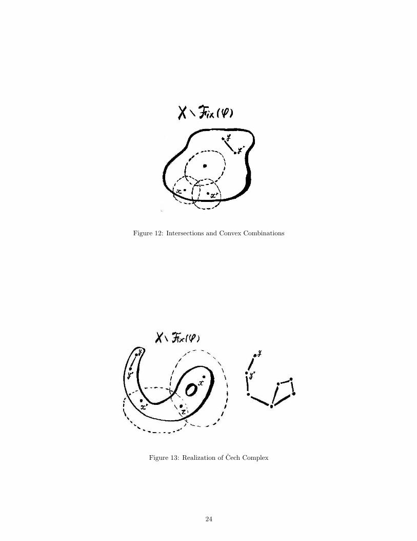
Figure 12: Intersections and Convex Combinations

Figure 13: Realization of Cech Complex

24

to the fixed point free convex extension of ϕ(x∗), so that x∗ cannot be any convex combination among points

y, y′, . . .. As we can see below, for such continuous mapping fϕ, the Lefschetz’s fixed point arguments may be

applicable, hence, for mapping ϕ of class scmathB, the trace of homology mapping fϕq : Hv

q (|K|)→ Hvq (|K|)

for each q = 0, 1, 2, . . ., of fϕ, (say, a certain kind of linear approximation of ϕ), is 0 for sufficiently fine K

as long as ϕ has no fixed point.

Convex Structures and Mappings of Class K

In the last part of Chapter 2 in Urai (2005), the author treated a wide class of mappings, the Kakutani

type, to which we have seen that (1) the fixed point property holds, and (2) a directional structure on which

the dual space representation of ϕ has local intersection property as long as ϕ has no fixed points may be

definable.

Assume that on space X there is a convex structure (DX , hX , {fA|A ∈ F(X)}). We say that a mapping,

ϕ : X → 2X \ {∅}, is of class K if for each x ∈ X , there is a closed convex set Kx such that (1) (x /∈

ϕ(x)) =⇒ (x /∈ Kx), and (2) there is an open neighborhood Ux of x satisfying that ∀z ∈ Ux, ϕ(z) ⊂ Kx.15

Note that for mapping ϕ of class K, each neighborhood Ux of x may be chosen arbitrarily small. Of course,

class K mapping is nothing but the Kakutani type mappings since for each mapping of the Kakutani type,

for all x ∈ Fix(ϕ), we may set Kx as Kx = X .

For mapping ϕ : X → X of class K, let us define the Lefschetz number of ϕ in a generalized sense. Since

X is compact and Hausdorff, for each mapping ϕ : X → 2X of class K, there is at least one covering

M = {M1, . . . ,Mm} of X such that for each i = 1, . . . ,m, there is a convex set Ki satisfying that (z ∈

Mi) =⇒ ϕ(z) ⊂ Ki. As stated above, M may be chosen arbitrarily small, so that we may suppose that

M 4 ∗N0, where N0 ∈ Cover(X) is the covering for lc space X stated in Theorem 3.4, (a). It is known

that the nerve of any covering N 4 ∗M4 ∗N0 gives the finite dimensional (ordinary simplicial) homology

group which is isomorphic to Hvn(X) for any dimension n. The isomorphism is induced by the composite

of mappings, ϕbN0n : Cc

n(∗N0)→ Cvn(N0), the projection p

∗N0M

n , ζbN

: Cvn(∗M) → Cc

n(M), and the inclusion

h∗MN

n to define the mapping between cycles as θn(z) = ϕbn ◦ pn ◦ ζb

n ◦ hn(z(N)). (See the proof of lemma 2

in Begle (1950b).)

Let N = {N1, . . . , Nn} be ∗M. Take a1 ∈ N1, . . . , an ∈ Nn and b1 ∈ ϕ(a1), . . ., bn ∈ ϕ(an) arbitrarily

and denote by A and B respectively the set {a1, . . . , an} and {b1, . . . , bn}. Denote by K(A) the complex

with vertices in A such that ai0 · · · ai`∈ K(A) iff

⋂`j=1 Nij

6= ∅. Clearly, K(A) is isomorphic to the nerve

of covering N, so that for an arbitrarily small refinement P of ∗N, there exists homomorphism θn between

cycles defining isomorphism between homology groups,

θn : Zvn(X)→ Zn(K(A))(9)

for any dimension n, where Zvn(X) denotes the set of all n-dimensional Vietoris cycles on X and θn(z) =

ϕbn ◦ pn ◦ ζb

n ◦ h∗NP

n (z(P)).

Since N is a star refinement of M, the complex, K(A), may be considered as a subcomplex of Xv(M).

Define an abstract complex, K(B), with the set of vertices, B, as bi0 · · · bi`∈ K(B) iff co{bij

: j = 0, . . . , `} ⊂

X . Then, we may obtain a simplicial mapping τ : K(A)→ K(B) such that τ(ai) = bi for each i = 1, . . . , n.

Moreover, under convex structure on X , by taking B ′ ⊃ B sufficiently large, the restriction of fB′ on

K(B), we may obtain a continuous mapping r on standard realization of K(B) into X . Hence, we have

homomorphism rn ◦ τn ◦ θn : Hvn(X)→ Hv

n(X) whose trace is well defined for each dimension n. Note that

15Since Kx is closed, we may suppose Ux ∩ Kx = ∅ without loss of generality as long as x /∈ Kx.

25

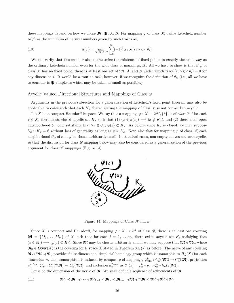
these mappings depend on how we chose M, P, A, B. For mapping ϕ of class K, define Lefschetz number

Λ(ϕ) as the minimum of natural numbers given by such traces as,

Λ(ϕ) = minM,P,A,B

∞∑

i=0

(−1)i trace (ri ◦ τi ◦ θi).(10)

We can verify that this number also characterize the existence of fixed points in exactly the same way as

the ordinary Lefschetz number even for the wide class of mappings, K. All we have to show is that if ϕ of

class K has no fixed point, there is at least one set of M, A, and B under which trace (ri ◦ τi ◦ θi) = 0 for

any dimension i. It would be a routine task, however, if we recognize the definition of θn (i.e., all we have

to consider is P-simplexes which may be taken as small as possible.)

Acyclic Valued Directional Structures and Mappings of Class D

Arguments in the previous subsection for a generalization of Lefschetz’s fixed point theorem may also be

applicable to cases such that each Kx characterizing the mapping of class K is not convex but acyclic.

Let X be a compact Hausdorff lc space. We say that a mapping, ϕ : X → 2X \{∅}, is of class D if for each

x ∈ X , there exists closed acyclic set Kx such that (1) (x /∈ ϕ(x)) =⇒ (x /∈ Kx), and (2) there is an open

neighborhood Ux of x satisfying that ∀z ∈ Ux, ϕ(z) ⊂ Kx. As before, since Kx is closed, we may suppose

Ux ∩Kx = ∅ without loss of generality as long as x /∈ Kx. Note also that for mapping ϕ of class K, each

neighborhood Ux of x may be chosen arbitrarily small. In standard cases, non-empty convex sets are acyclic,

so that the discussion for class D mapping below may also be considered as a generalization of the previous

argument for class K mappings (Figure 14).

Figure 14: Mappings of Class K and D

Since X is compact and Hausdorff, for mapping ϕ : X → 2X of class D, there is at least one covering

M = {M1, . . . ,Mm} of X such that for each i = 1, . . . ,m, there exists acyclic set Ki satisfying that

(z ∈Mi) =⇒ (ϕ(z) ⊂ Ki). Since M may be chosen arbitrarily small, we may suppose that M 4N0, where

N0 ∈ Cover(X) is the covering for lc space X stated in Theorem 3.4 (a) as before. The nerve of any covering

N4 ∗∗M 4N0 provides finite dimensional simplicial homology group which is isomorphic to Hvn(X) for each

dimension n. The isomorphism is induced by composite of mappings, ϕbMn : Cc

n(∗M)→ Cvn(M), projection

pM∗M

n , ζb∗M

: Cvn(∗∗M)→ Cc

n(∗M), and inclusion h∗∗

MN

n as θn(z) = ϕbn ◦ pn ◦ ζb

n ◦ hn(z(N)).

Let k be the dimension of the nerve of N. We shall define a sequence of refinements of N

M0 4 M1 4 · · ·4Mk−1 4Mk 4Mk+1 4N 4 ∗∗M4 ∗M 4 M4 N0(11)

26

as follows: Let Mk+1 = N. For ` such that 0 ≤ ` ≤ k, define M` as a refinement of ∗∗M`+1 such that

for each compact acyclic Ki ∈ {K1, . . . ,Km}, any `-dimensional Vietoris M`-cycle of Ki bounds a chain

in M`+1 of Ki. (This is always possible by Theorem 3.2.) Note that for each pair of M` and M`+1 and

dimension n, homomorphism θ`+1`n = ϕb

n ◦ pn ◦ ζbn ◦ hn between Cv

n(M`+1) and Cvn(M`) which induces the

isomorphism among homology groups exists.

Let us define a chain homomorphism τ = {τq} on the k-skeleton of Xv(M0) to Xv(N). At first, denote by

L = {L0, L1, . . . , Ls} the cover ∗M. By definition of ϕbMn, ϕb

Mn(Li) = xLi∈ Li and there exists an Mj ∈M

such that St(Li; L) ⊂ Mj . Define ai as ai = xLiand Kai

as the corresponding Kj for each i = 0, . . . , s.

Then we have for each x ∈ Li, ϕ(x) ⊂ Kaifor all i. With respect to ai, fix a point bi ∈ ϕ(ai) ⊂ Kai

for each

i.

For 0-dimensional simplex σ0 = 〈x0〉 of Xv(M0), the image θ0 ◦ θn+1n0 ◦ · · · ◦ θ100 (x0) is by definition one

of points a0, . . . , as, say ai. Define τ0(σ0) as τ0(σ

0) = bi and extend it linearly on Cv0 (M0) to Cv

0 (M0) ⊂

Cv0 (M).

Next, for 1-dimensional simplex σ1 = 〈x0x1〉 of Xv(M0), we may write τ0∂(σ1) = τ0(x0 − x1) as bi − bj ,

where bi = τ0(x0) and bj = τ0(x

1). Of course, bi− bj may also be considered as an M0-cycle (in the reduced

sense).16 Hence, by definition of M0 relative to M1, we have a M1-chain c1 such that ∂(c1) = bi − bj

Figure 15: Class D mapping and M1-chain

(Figure 15). Define τ1(σ1) as τ1(σ

1) = c1 and extend it linearly on Cv1 (M0) to Cv

1 (M1) ⊂ Cv1 (M). Clearly,

∂τ1 = τ0∂ holds.

Now, assume that for all dimension q < `, (2 ≤ ` ≤ k), τq is defined on Cvq (M0) to Cv

q (Mq) ⊂ Cvq (M)

and ∂τq = τq−1∂ holds. Then for `-dimensional simplex σ` of Xv(M0), chain c = τ`−1∂(σ`) is well defined.

Since ∂(c) = ∂τ`−1∂(σ`) = τ`−2∂∂(σ`) = 0, c is indeed M`−1-cycle. Hence, by definition of M`−1 relative

to M`, we have a M`-chain c` such that ∂(c`) = c. Define τ`(σ`) as τ`(σ

`) = c` and extend it linearly on

Cv` (M0) to Cv

` (M`) ⊂ Cv1 (M). Clearly, ∂τ` = τ`−1∂ holds.

Hence, by induction, we have successfully obtained the chain map τ = {τq} on the k-skeleton of Xv(M0)

to Xv(Mk+1) = Xv(N) ⊂ Xv(M), i.e., we have

τq : Cvq (M0)→ Cv

q (N) ⊂ Cvq (M)(12)

16Every point of X may be considered as a 0-dimensional M0-simplex. Note also that in Theorem 3.2, 0-dimensional cyclesshould be taken in the reduced sense.

27

for all q = 0, 1, . . . , k. The homology groups of Xv(M0) and Xv(N) are isomorphic under the isomorphism

induced by θn+1n◦· · ·◦θ10. Since both of them are isomorphic to the corresponding group of a finite complex,

trace (τq) is well defined for all q and∑∞

i=0(−1)i trace (τi) is finite. Though definition of τ depends on M,

N, and, especially, set A of all ai’s and B of all bi’s, we may define as before the minimum of such values,

Λ(ϕ) = minM,N,A,B

∞∑

i=0

(−1)i trace (τi)(13)

as an extended Lefschetz number for mapping ϕ of class D. By considering the definition of θ`+1`n ’s, we

obtain the following extension of Lefschetz’s fixed point theorem.

Theorem 6.1 : (Extension of Lefschetz’s Fixed Point Theorem) Let X be a compact Hausdorff lc space.

Mapping ϕ of class D has a fixed point if Λ(ϕ) 6= 0.

REFERENCES

Begle, E. G. (1950): “A fixed point theory,” Annals of Mathematics 51(3), 544–550.

Begle, E. G. (1950): “The Vietoris mapping theorem for bicompact spaces,” Annals of Mathematics 51(3),

534–543.

Cech, E. (1932): “Theorie generale de l’homologie dans une espace quelconque,” Fund. Math. 19, 149–183.

Debreu, G. (1959): Theory of Value. Yale University Press, New Haven, CT.

Eilenberg, S. and Montgomery, D. (1946): “Fixed point theorems for multi-valued transformations,” Amer-

ican Journal of Mathematics 68, 214–222.

Eilenberg, S. and N.Steenrod, (1952): Foundations of Algebraic Topology. Princeton University Press, Prince-

ton, New Jersey.

Hocking, J. G. and Young, G. S. (1961): Topology. Dover Publications, Inc., New York.

Lefschetz, S. (1937): “On the fixed point formula,” Annals of Mathematics 38(4), 819–822.

Lefschetz, S. (1942): Algebraic Topology vol. 27. Amer. Math. Soc. Colloquium Publications, New York.

Nikaido, H. (1959): “Coincidence and some systems of inequalities,” Journal of The Mathematical Society

of Japan 11(4), 354–373.

Nikaido, H. (1968): Convex Structures and Economic Theory. Academic Press, New York.

Steenrod, N. E. (1936): “Universal Homology Groups,” Amer. J. Math 58, 661–701.

Tukey, J. W. (1940): Convergence and Uniformity in Topology. Princeton University Press.

Urai, K. (2005): “Fixed Points and Economic Equilibria,” Ph.D. Thesis, Osaka University.

Vietoris, L. (1927): “Uber den hoheren Zusammenhang kompakter Raume und eine Klasse von zusammen-

hangstreuen Abbildungen,” Mathematische Annalen 97, 454–472.

28