homomesy of order ideals in products of two chains - university of
TRANSCRIPT

Homomesy of Order Ideals in Products ofTwo Chains
Tom Roby (University of Connecticut)
Describing joint research with Jim Propp
Combinatorics SeminarUniversity of MinnesotaMinneapolis, MN USA
6 Sept 2013
Slides for this talk are available online (or will be soon) at
http://www.math.uconn.edu/~troby/research.html

Abstract
We consider a variety of combinatorial actions on finite sets, e.g.,cyclic rotation of binary strings, promotion of Young tableaux androwmotion on order ideals of partially ordered sets. We identify aparticular phenomenon called “homomesy” appearing in manyunrelated combinatorial contexts: namely that the average value ofsome natural statistic over each orbit is the same as the averageover the entire set. Viewing these actions as products of “toggleoperations” allows us to see how some of these actions are relatedand to extend much of this picture more broadly. In particular, wecan generalize the operations of rowmotion and promotion (Strikerin and Williams’s terminology) on order ideals in a poset to (1) theorder polytope of a poset (the continuous piecewise-linearcategory), and (2) to the collection of maps from a poset P torational functions in |P| variables (the birational category).

Acknowledgments
This talk largely discusses recent work with Jim Propp, includingideas and results from Arkady Berenstein, David Einstein,Shahrzad Haddadan, Jessica Striker, and Nathan Williams.
Darij Grinberg wrote invaluable Sage code to compute birationalpromotion. Mike LaCroix wrote fantastic postscript code togenerate animations and pictures that illustrate our mapsoperating on order ideals on products of chains. Jim Propp createdmany of the other pictures and slides that are used here.
Thanks also to Omer Angel, Drew Armstrong, Anders Bjorner,Barry Cipra, Karen Edwards, Robert Edwards, Svante Linusson,Vic Reiner, Richard Stanley, Ralf Schiffler, Hugh Thomas, PeteWinkler, and Ben Young.

Overview
Rotation of bit-strings;
Unexpected averaging properties: homomesic statistics;
Suter’s dihedral symmetries in Young’s lattice;
Rowmotion and Promotion actions on antichains and orderideals of posets;
Homomesic statistics for actions in [a]× [b];
Generalizing to other actions on order polytopes and rationalfunctions;
Please interrupt with questions!

Example 1: Rotation of bit-strings
Let S denote the set of length n binary strings with exactly k 1’s.and set τ := CR : S → S by b = b1b2 · · · bn 7→ bnb1b2 · · · bn−1(cyclic shift). Let ϕ(b) = #inversions(b) = #{i < j : bi > bj}.Then over any τ -orbit O we have:
1
#O∑s∈O
ϕ(s) =k(n − k)
2=
1
#S
∑s∈S
ϕ(s).
EG: n = 4, k = 2 gives us two orbits:
0011 0101
1001 10101100 010101100011

Example 1: Rotation of bit-strings
Let S denote the set of length n binary strings with exactly k 1’s.and set τ := CR : S → S by b = b1b2 · · · bn 7→ bnb1b2 · · · bn−1(cyclic shift). Let ϕ(b) = #inversions(b) = #{i < j : bi > bj}.Then over any τ -orbit O we have:
1
#O∑s∈O
ϕ(s) =k(n − k)
2=
1
#S
∑s∈S
ϕ(s).
EG: n = 4, k = 2 gives us two orbits:
0011 0101
1001 7→ 2 1010 7→ 31100 7→ 4 0101 7→ 10110 7→ 20011 7→ 0

Example 1: Rotation of bit-strings
Let S denote the set of length n binary strings with exactly k 1’s.and set τ := CR : S → S by b = b1b2 · · · bn 7→ bnb1b2 · · · bn−1(cyclic shift). Let ϕ(b) = #inversions(b) = #{i < j : bi > bj}.Then over any τ -orbit O we have:
1
#O∑s∈O
ϕ(s) =k(n − k)
2=
1
#S
∑s∈S
ϕ(s).
EG: n = 4, k = 2 gives us two orbits:
0011 0101
1001 7→ 2 1010 7→ 31100 7→ 4 0101 7→ 10110 7→ 2 AVG = 4
2 = 20011 7→ 0
AVG = 84 = 2

More rotation
EG: n = 6, k = 2 gives us three orbits:
000011 000101 001001
100001 100010 100100110000 010001 010010011000 101000 001001001100 010100000110 001010000011 000101

More rotation
EG: n = 6, k = 2 gives us three orbits:
000011 000101 001001
100001 100010 100100110000 010001 010010011000 101000 001001001100 010100000110 001010000011 000101

More rotation
EG: n = 6, k = 2 gives us three orbits:
000011 000101 001001
100001 100010 100100110000 010001 010010011000 101000 001001001100 010100000110 001010000011 000101

More rotation
EG: n = 6, k = 2 gives us three orbits:
000011 000101 001001
100001 7→ 4 100010 7→ 5 100100 7→ 6110000 7→ 8 010001 7→ 3 010010 7→ 4011000 7→ 6 101000 7→ 7 001001 7→ 2001100 7→ 4 010100 7→ 5000110 7→ 2 001010 7→ 3000011 7→ 0 000101 7→ 1

More rotation
EG: n = 6, k = 2 gives us three orbits:
000011 000101 001001
100001 7→ 4 100010 7→ 5 100100 7→ 6110000 7→ 8 010001 7→ 3 010010 7→ 4011000 7→ 6 101000 7→ 7 001001 7→ 2001100 7→ 4 010100 7→ 5000110 7→ 2 001010 7→ 3000011 7→ 0 000101 7→ 1
AVG = 246 = 4 AVG = 24
6 = 4 AVG = 123 = 4

More rotation
EG: n = 6, k = 2 gives us three orbits:
000011 000101 001001
100001 7→ 4 100010 7→ 5 100100 7→ 6110000 7→ 8 010001 7→ 3 010010 7→ 4011000 7→ 6 101000 7→ 7 001001 7→ 2001100 7→ 4 010100 7→ 5000110 7→ 2 001010 7→ 3000011 7→ 0 000101 7→ 1
AVG = 246 = 4 AVG = 24
6 = 4 AVG = 123 = 4
We know two simple ways to prove this: one can show pictoriallythat the value of the sum doesn’t change when you mutate b(replacing a 01 somewhere in b by 10 or vice versa), or one canwrite the number of inversions in b as
∑i<j bi (1− bj) and then
perform algebraic manipulations.

Main definition: Homomesic
MAIN DEF: Given an (invertible) action τ on a finite set ofobjects S , call a statistic ϕ : S → C homomesic with respect to(S , τ) iff the average of ϕ over each τ -orbit O is the same for all
O, i.e.,1
#O∑s∈O
ϕ(s) does not depend on the choice of O.
Equivalently: the average of ϕ over each τ -orbit O is the same asthe average over the entire set S :
1
#O∑s∈O
ϕ(s) =1
#S
∑s∈S
ϕ(s).
So in looking for homomesic statistics we can compute what theaverage should be before checking whether a statistic ishomomesic.

Semi-Standard Young Tableaux
Fix a positive integer N. A semi-standard Young tableau(SSYT) of shape λ and ceiling N is a labeling of the cells of theYoung diagram of a partition λ with numbers from 1, 2, . . . ,Nwhich increases weakly along each row and strictly along eachcolumn. For example,
1 1 2 4
2 3 4
4 4 ,
1 1 1 2 2 5
4 4 4 5
5 5 6 but not
1 1 2 2 3 3
2 3 4 4
3 4 4
The weight vector α(T ) = (α1, α2, . . . , αN) is given byαi := αi (T ) = #occurrences of i in T . EG, the weight vectors forthe two tableaux above are (2, 2, 1, 4) and (3, 2, 0, 3, 4, 1).
We let SSYT (λ,N) denote the set of all semi-standard Youngtableaux whose entries lie within [N] = {1, 2, . . .N}.

Bender-Knuth involutions
A standard method for proving combinatorially that Schurfunctions are symmetric is to use Bender-Knuth involutions.Given T ∈ SSYT (λ,N) and i ∈ [N − 1], consider all the i ’s thatappear above an i + 1 in the same column, and all the i + 1’s thatappear below an i in the same column to be married and theremainder free. Then in each row with r free i ’s and s free i + 1’s,βi replaces these with s free i ’s and r free i + 1’s.
ii i i i︸︷︷︸ i + 1 i + 1 i + 1 i + 1︸ ︷︷ ︸ i + 1
i + 1 i + 1 r=2 s=4
i7→ i i i i i i︸ ︷︷ ︸ i + 1 i + 1︸ ︷︷ ︸ i + 1
i + 1 i + 1 s=4 r=2

Promotion of SSYT via Bender-Knuth involutions
Define the following operator on SSYT (λ,N):
∂ := βN−1 ◦ βN−2 ◦ · · · ◦ β2 ◦ β1 ,
the composition of all BK involutions in order. By a result ofGansner [Gan80], this operator coincides with Schutzenberger’spromotion operator. Then for all i ∈ [N], the weight vectorcoordinate αi (T ) is homomesic w.r.t. ∂ acting on SSYT (λ,N).
EG: Let N = 5 and T =1 1 1 2 2 3 3 3 42 2 3 3 4 4 53 4 4 5
Then the content vectors α = [α1, α2, . . . , αN ] that arise as wesuccessively apply βi ’s behave as follows, starting from [3, 4, 6, 5, 2]:
[4, 3, 6, 5, 2] [6, 4, 5, 2, 3] [5, 6, 2, 3, 4] [2, 5, 3, 4, 6] [3, 2, 4, 6, 5][4, 6, 3, 5, 2] [6, 5, 4, 2, 3] [5, 2, 6, 3, 4] [2, 3, 5, 4, 6] [3, 4, 2, 6, 5][4, 6, 5, 3, 2] [6, 5, 2, 4, 3] [5, 2, 3, 6, 4] [2, 3, 4, 5, 6] [3, 4, 6, 2, 5][4, 6, 5, 2, 3] [6, 5, 2, 3, 4] [5, 2, 3, 4, 6] [2, 3, 4, 6, 5] [3, 4, 6, 5, 2]
An easy homomesy for Promotion
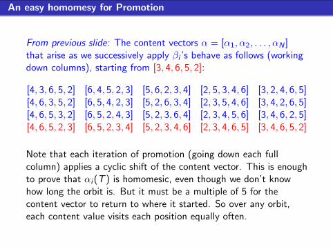
From previous slide: The content vectors α = [α1, α2, . . . , αN ]that arise as we successively apply βi ’s behave as follows (workingdown columns), starting from [3, 4, 6, 5, 2]:
[4, 3, 6, 5, 2] [6, 4, 5, 2, 3] [5, 6, 2, 3, 4] [2, 5, 3, 4, 6] [3, 2, 4, 6, 5][4, 6, 3, 5, 2] [6, 5, 4, 2, 3] [5, 2, 6, 3, 4] [2, 3, 5, 4, 6] [3, 4, 2, 6, 5][4, 6, 5, 3, 2] [6, 5, 2, 4, 3] [5, 2, 3, 6, 4] [2, 3, 4, 5, 6] [3, 4, 6, 2, 5][4, 6, 5, 2, 3] [6, 5, 2, 3, 4] [5, 2, 3, 4, 6] [2, 3, 4, 6, 5] [3, 4, 6, 5, 2]
Note that each iteration of promotion (going down each fullcolumn) applies a cyclic shift of the content vector. This is enoughto prove that αi (T ) is homomesic, even though we don’t knowhow long the orbit is. But it must be a multiple of 5 for thecontent vector to return to where it started. So over any orbit,each content value visits each position equally often.

An easy homomesy for Promotion
From previous slide: The content vectors α = [α1, α2, . . . , αN ]that arise as we successively apply βi ’s behave as follows (workingdown columns), starting from [3, 4, 6, 5, 2]:
[4, 3, 6, 5, 2] [6, 4, 5, 2, 3] [5, 6, 2, 3, 4] [2, 5, 3, 4, 6] [3, 2, 4, 6, 5][4, 6, 3, 5, 2] [6, 5, 4, 2, 3] [5, 2, 6, 3, 4] [2, 3, 5, 4, 6] [3, 4, 2, 6, 5][4, 6, 5, 3, 2] [6, 5, 2, 4, 3] [5, 2, 3, 6, 4] [2, 3, 4, 5, 6] [3, 4, 6, 2, 5][4, 6, 5, 2, 3] [6, 5, 2, 3, 4] [5, 2, 3, 4, 6] [2, 3, 4, 6, 5] [3, 4, 6, 5, 2]
Note that each iteration of promotion (going down each fullcolumn) applies a cyclic shift of the content vector. This is enoughto prove that αi (T ) is homomesic, even though we don’t knowhow long the orbit is. But it must be a multiple of 5 for thecontent vector to return to where it started. So over any orbit,each content value visits each position equally often.

A small example of promotion
(taken from J. Striker and N. Williams, Promotion andRowmotion, European J. Combin. 33 (2012), no. 8, 1919–1942;http://arxiv.org/abs/1108.1172):

A small example of promotion: centrally symmetric sums

Promotion of Semi-Standard Young Tableaux: homomesies
Conjecture
Let S be the set of Semi-Standard Young Tableaux of rectangularshape λ and ceiling N. If c and c ′ are opposite cells, i.e., c and c ′
are related by 180-degree rotation about the center (note: the casec = c ′ is permitted when λ is odd-by-odd), and ϕ(T ) denotes thesum of the numbers in cells c and c ′, then ϕ is homomesic withrespect to (S , ∂) with average value N + 1.
This has recently been proven by J. Bloom, O. Pechenik, &D. Saracino, http://arxiv.org/abs/1308.0546, using a growthdiagram argument and separately by jeu de taquin. The firstargument generalizes to the analogous result for “cominuusculeposets”.

Cominuscule Posets
The first three pictures represent infinite classes; while the last twoare sporadic. (Picture from [BPS13].)

Example 4: Suter’s symmetries
Let YN be the set of number-partitions λ whose maximal hooklengths are strictly less than N (i.e., whose Young diagrams fitinside some rectangle that fits inside the staircase shape(N − 1,N − 2, ..., 2, 1)).
Suter showed that the Hasse diagram of YN has N-fold cyclicsymmetry (indeed, N-fold dihedral symmetry) by exhibiting anexplicit action of order N.

Suter’s action, N = 5
(taken from R. Suter, Young’s lattice and dihedral symmetriesrevisited: Mobius strips and metric geometry ;http://arxiv.org/abs/1212.4463):

Suter’s action, N = 5: weighted sums

Suter’s action: homomesies
Assign weight 1 to the cells at the diagonal boundary of thestaircase shape, weight 2 to their neighbors, ..., and weight N − 1to the cell at the lower left, and for λ ∈ YN let ϕ(λ) be the sum ofthe weights of all the cells in the Young diagram of λ.
Prop. (Einstein-Propp): ϕ is homomesic under Suter’s map withaverage value (N3 − N)/12.
More refined result: If i + j = N (note: i = j is permitted), andϕi ,j(λ) is the sum of the weights of all the cells in λ with weight iplus the sum of the weights of all the cells in λ with weight j , thenϕi ,j is homomesic under Suter’s map with average ij in all orbits.

Rowmotion: an invertible operation on antichains
Given A ∈ A(P), let τ(A) be the set of minimal elements of thecomplement of the order ideal generated by A.τ is invertible since it is a composition of three invertibleoperations:
antichains←→ down-sets←→ up-sets←→ antichains
We can also view this as an invertible action τ on J(P), the set oforder ideals of P, via the above isomorphism between A(P) andJ(P); in other words, perform the above steps in the order 2,3,1.
This map and its inverse have been considered with varyingdegrees of generality, by many people more or less independently(using a variety of nomenclatures and notations): Duchet, Brouwerand Schrijver, Cameron and Fon Der Flaass, Fukuda, Panyushev,Rush and Shi, and Striker and Williams [SW12]. Following[SW12], we call this rowmotion.

An example
1. Saturate downward
2. Complement
3. Take minimal element(s)
1−→ 2−→ 3−→
1

Example in lattice cell form
Viewing the elements of the poset as squares, we would map:
Area = 8
X X
τ−→τ−→
Area = 10
X
X X

Panyushev’s conjecture
Let ∆ be a reduced irreducible root system in Rn. (Pictures soon!)Choose a system of positive roots and make it a poset of rank n bydecreeing that y covers x iff y − x is a simple root.Conjecture (Conjecture 2.1(iii) in D.I. Panyushev, On orbits ofantichains of positive roots, European J. Combin. 30 (2009),586-594): Let O be an arbitrary τ -orbit. Then
1
#O∑A∈O
#A =n
2.
In our language, the cardinality statistic is homomesic with respectto the action of rowmotion on antichains in root posets.
Panyushev’s Conjecture 2.1(iii) (along with much else) was provedby Armstrong, Stump, and Thomas in their article A uniformbijection between nonnesting and noncrossing partitions,http://arxiv.org/abs/1101.1277.

Picture of root posets
Here are the classes of posets included in Panyushev’s conjecture.
(Graphic courtesy of Striker-Williams.)

Panyushev’s conjecture: The An case, n = 2
Here we have just an orbit of size 2 and an orbit of size 3:
0 2 1
1 1
1
Within each orbit, the average antichain has cardinality n/2 = 1.

The case A3.
Here’s an example orbit taken from [AST] for the A3 root poset:
For A3 this action has three orbits (sized 2, 4, and 8), and theaverage cardinality of an antichain is
1
8(2 + 1 + 1 + 2 + 2 + 1 + 1 + 2) =
3
2=
n
2

Antichains in [a]× [b]: cardinality is homomesic
A simpler-to-prove phenomenon of this kind concerns the poset[a]× [b] (where [k] denotes the linear ordering of {1, 2, . . . , k}):
Theorem (Propp, R.)
Let O be an arbitrary τ -orbit in A([a]× [b]). Then
1
#O∑A∈O
#A =ab
a + b.
This is an easy consequence of unpublished work of Hugh Thomasbuilding on earlier work of Richard Stanley: see the last paragraphof section 2 of R. Stanley, Promotion and evacuation,http://www.combinatorics.org/ojs/index.php/eljc/
article/view/v16i2r9 .

Antichains in [a]× [b]: the case a = b = 2
Here we have an orbit of size 2 and an orbit of size 4:
Within each orbit, the average antichain has cardinalityab/(a + b) = 1.
0 1 2 1
1 1
1

Antichains in [a]× [b]: fiber-cardinality is homomesic
0 0 0 1 1 1 1 0
1 0 0 1
1
Within each orbit, the average antichain has1/2 a green element and 1/2 a blue element.

Antichains in [a]× [b]: fiber-cardinality is homomesic
For (i , j) ∈ [a]× [b], and A an antichain in [a]× [b], let 1i ,j(A) be1 or 0 according to whether or not A contains (i , j).
Also, let fi (A) =∑
j∈[b] 1i ,j(A) ∈ {0, 1} (the cardinality of theintersection of A with the fiber {(i , 1), (i , 2), . . . , (i , b)} in[a]× [b]), so that #A =
∑i fi (A).
Likewise let gj(A) =∑
i∈[a] 1i ,j(A), so that #A =∑
j gj(A).
Theorem (Propp, R.)
For all i , j ,
1
#O∑A∈O
fi (A) =b
a + band
1
#O∑A∈O
gj(A) =a
a + b.
The indicator functions fi and gj are homomesic under τ , eventhough the indicator functions 1i ,j aren’t.

Antichains in [a]× [b]: centrally symmetric homomesies
Theorem (Propp, R.)
In any orbit, the number of A that contain (i , j) equals the numberof A that contain the opposite element(i ′, j ′) = (a + 1− i , b + 1− j).
That is, the function 1i ,j − 1i ′,j ′ is homomesic under τ , withaverage value 0 in each orbit.

Linearity
Useful triviality: every linear combination of homomesies is itselfhomomesic.
E.g., consider the adjusted major index statistic defined byamaj(A) =
∑(i ,j)∈A(i − j).
Propp and R. proved that amaj is homomesic under τby writing it as a linear combination of the functions 1i ,j − 1i ′,j ′ .Haddadan gave a simpler proof,writing amaj as a linear combination of the functions fi and gj .
Question: Are there other homomesic combinations of theindicator functions 1i ,j (with (i , j) ∈ [a]× [b]),linearly independent of the functions fi , gj , and 1i ,j − 1i ′,j ′?

Ideals in [a]× [b]: cardinality is homomesic
As we’ve seen, one can view rowmotion as acting either onantichains (A(P)) or on order ideals (J(P)); we denote the lattermap τ . It turns out that the cardinality of the order ideal is alsohomomesic with respect to rowmotion on [a]× [b].
Theorem (Propp, R.)
Let O be an arbitrary τ -orbit in J([a]× [b]). Then
1
#O∑I∈O
#I =ab
2.
It’s worth noting even though there’s a strong connection betweenthe rowmotion map on antichains and on order ideals, that thehomomesy situation could be quite different.

One action, two vector spaces
The map τ is “the same” as τ in the sense that the standardbijection from A(P) to J(P) (downward saturation) makes thefollowing diagram commute:
A(P)τ−→ A(P)
↓ ↓J(P)
τ−→ J(P)
However, the bijection from A(P) to J(P) does not carry thevector space generated by the functions 1i ,j to the vector spacegenerated by the functions 1i ,j in a linear way.
So the homomesy situation for τ : J(P)→ J(P) could be(and, as we’ll see, is) different from the homomesy situation forτ : A(P)→ A(P).

Rowmotion on [4]× [2] A

Rowmotion on [4]× [2] A
1
Area = 0
2
Area = 1
3
Area = 3
4
Area = 5
5
Area = 7
6
Area = 8
(0+1+3+5+7+8) / 6 = 4

Rowmotion on [4]× [2] B

Rowmotion on [4]× [2] B
1
Area = 2
2
Area = 4
3
Area = 6
4
Area = 6
5
Area = 4
6
Area = 2
(2+4+6+6+4+2) / 6 = 4

Rowmotion on [4]× [2] C

Rowmotion on [4]× [2] C
1
Area = 3
2
Area = 5
3
Area = 4
4
Area = 3
5
Area = 5
6
Area = 4
(3+5+4+3+5+4) / 6 = 4

Ideals in [a]× [b]: the case a = b = 2
Again we have an orbit of size 2 and an orbit of size 4:
Within each orbit, the average order ideal has cardinality ab/2 = 2.
0 1 3 4
2 2
1

Ideals in [a]× [b]: file-cardinality is homomesic
We also have homomesies for more refined statistics than #I .
0 0 0 0 1 0 1 1 1 1 2 1
1 1 0 0 1 1
1
Within each orbit, the average order ideal has1/2 a violet element, 1 red element, and 1/2 a brown element.

Ideals in [a]× [b]: file-cardinality is homomesic
For 1− b ≤ k ≤ a− 1, define the kth file of [a]× [b] as
{(i , j) : 1 ≤ i ≤ a, 1 ≤ j ≤ b, i − j = k}.
For 1− b ≤ k ≤ a− 1, let hk(I ) be the number of elements of I inthe kth file of [a]× [b], so that #I =
∑k hk(I ).
Theorem (Propp, R.)
For every τ -orbit O in J([a]× [b]),
1
#O∑I∈O
hk(I ) =
{(a−k)ba+b if k ≥ 0
a(b+k)a+b if k ≤ 0.

Ideals in [a]× [b]: centrally symmetric homomesies
Given (i , j) ∈ [a]× [b], and I an ideal in [a]× [b], define theindicator function 1i ,j(I ) to be 1 or 0 according to whether or not Icontains (i , j).
Write (i ′, j ′) = (a + 1− i , b + 1− j), the point opposite (i , j) in theposet.
Theorem (Propp, R.)
1i ,j + 1i ′,j ′ is homomesic under τ .

The two vector spaces, compared
In the space associated with antichains:fiber-cardinalities andcentrally symmetric differences
are homomesic.
In the space associated with order ideals:file-cardinalities andcentrally symmetric sums
are homomesic.
Note that the the discovery of these homomesies was driven bycalculation, and the project of generalizing these results to otherposets will clearly be aided by computer-assisted search.

Toggling
In their 1995 article Orbits of antichains revisited , European J.Combin. 16 (1995), 545–554, Cameron and Fon-der-Flaass give analternative description of τ .
Given I ∈ J(P) and x ∈ P, let τx(I ) = I4{x} (symmetricdifference) provided that I4{x} is an order ideal of P; otherwise,let τx(I ) = I .
We call the involution τx “toggling at x”.
The involutions τx and τy commute unless x covers y or y covers x .

An example
1. Toggle the top element
2. Toggle the left element
3. Toggle the right element
4. Toggle the bottom element
1−→ 2−→ 3−→ 4−→
1
Toggling from top to bottom
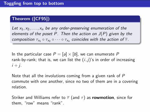
Theorem ([CF95])
Let x1, x2, . . . , xn be any order-preserving enumeration of theelements of the poset P. Then the action on J(P) given by thecomposition τx1 ◦ τx2 ◦ · · · ◦ τxn coincides with the action of τ .
In the particular case P = [a]× [b], we can enumerate Prank-by-rank; that is, we can list the (i , j)’s in order of increasingi + j .
Note that all the involutions coming from a given rank of Pcommute with one another, since no two of them are in a coveringrelation.
Striker and Williams refer to τ (and τ) as rowmotion, since forthem, “row” means “rank”.

Toggling from side to side
Recall that a file in P = [a]× [b] is the set of all (i , j) ∈ P withi − j equal to some fixed value k .
Note that all the involutions coming from a given file commutewith one another, since no two of them are in a covering relation.
It follows that for any enumeration x1, x2, . . . , xn of the elements ofthe poset [a]× [b] arranged in order of increasing i − j , the actionon J(P) given by τx1 ◦ τx2 ◦ · · · ◦ τxn doesn’t depend on whichenumeration was used.
Striker and Williams call this well-defined composition promotion,and denote it by ∂, since for two-rowed tableaux it can be relatedto Schutzenberger’s promotion on SYT, described earlier.

Promoting ideals in [a]× [b]: the case a = b = 2
Again we have an orbit of size 2 and an orbit of size 4:
0 2 4 2
1 3
1

J([a]× [b]): cardinality is homomesic under promotion
Theorem (Propp, R.)
Let O be an arbitrary orbit in J([a]× [b]) under the action ofpromotion ∂. Then
1
#O∑I∈O
#I =ab
2.
The result about cyclic rotation of binary words discussed earlierturns out to be a special case of this.

J([a]× [b]): file-cardinality is homomesic under promotion
For 1− b ≤ k ≤ a− 1, let fk(I ) be the number of elements of I inthe kth file of [a]× [b], so that #I =
∑k fk(I ).
Theorem
If O is any ∂-orbit in J([a]× [b]),
1
#O∑I∈O
fk(I ) =
{(a−k)ba+b if k ≥ 0
a(b+k)a+b if k ≤ 0.

A([a]× [b]) under promotion
Cardinality of antichains is not homomesic under promotion.although the antipodal functions 1i ,j − 1i ′,j ′ are.

Root posets of type A: antichains
Recall that, by the Armstrong-Stump-Thomas theorem, thecardinality of antichains is homomesic under the action ofrowmotion, where the poset P is a root poset of type An.E.g., for n = 2:
Antichain-cardinality is homomesic: in each orbit, its average is 1.
0 2 1
1 1
1

Root posets of type A: order ideals
What if instead of antichains we take order ideals?
E.g., n = 2:
What is homomesic here?
1

Root posets of type A: rank-signed cardinality
0 2 1
1 1
+ + + +
+ +
−
1

Root posets of type A: rank-signed cardinality is homomesic
Theorem (Haddadan)
Let P be the root poset of type An. If we assign an element x ∈ P
weight wt(x) = (−1)rank(x), and assign an order ideal I ∈ J(P)weight ϕ(I ) =
∑x∈I wt(x), then ϕ is homomesic under rowmotion
and promotion, with average n/2.

The order polytope of a poset
Let P be a poset, with an extra minimal element 0 and an extramaximal element 1 adjoined.
The order polytope O(P) (introduced by R. Stanley) is the set offunctions f : P → [0, 1] with f (0) = 0, f (1) = 1, and f (x) ≤ f (y)whenever x ≤P y .We can generalize our entire setup of toggle operators and“rowmotion” to operate on these functions (the “continuouspiecewise-linear (CPL) category”).

Flipping-maps in the order polytope
For each x ∈ P, define the flip-map σx : O(P)→ O(P) sending fto the unique f ′ satisfying
f ′(y) =
{f (y) if y 6= x ,minz ·>x f (z) + maxw<· x f (w)− f (x) if y = x ,
where z ·>x means z covers x and w< · x means x covers w .
Note that the interval [minz ·>x f (z),maxw<· x f (w)] is preciselythe set of values that f ′(x) could have so as to satisfy theorder-preserving condition, if f ′(y) = f (y) for all y 6= x ;the map that sends f (x) to minz ·>x f (z) + maxw<· x f (w)− f (x)is just the affine involution that swaps the endpoints.

Example of flipping at a node
w1 w2
x
z1 z2
.1 .2
.4
.7 .8
−→
.1 .2
.5
.7 .8
1
minz ·>x
f (z) + maxw<· x
f (w) = .7 + .2 = .9
f (x) + f ′(x) = .4 + .5 = .9

Flipping and toggling
If we associate each order-ideal I with the indicator function f ofP \ I (that is, the function that takes the value 0 on I and thevalue 1 everywhere else), then toggling I at x is tantamount toflipping f at x .
That is, we can identify J(P) with the vertices of the polytopeO(P) in such a way that toggling can be seen to be a special caseof flipping.
This may be clearer if you think of J(P) as being in bijection withthe set of monotone 0,1-valued functions on P.

Flipping
Flipping (at least in special cases) is not new, though it is notwell-studied; the most worked-out example we’ve seen isBerenstein and Kirillov’s article Groups generated by involutions,Gelfand-Tsetlin patterns and combinatorics of Young tableaux (St.Petersburg Math. J. 7 (1996), 77–127); seehttp://pages.uoregon.edu/arkadiy/bk1.pdf.

Composing flips
Just as we can apply toggle-maps from top to bottom, we canapply flip-maps from top to bottom (successively at the North,West, East, and South.) :
.8
8888 .6
8888 .6
8888
.4
����.3
����
σN
→ .4
����.3
����
σW
→ .3
����.3
����
.1
8888
.1
8888
.1
8888
.6
8888 .6
8888
σE
→ .3
����.4
����
σS
→ .3
����.4
����
.1
8888
.2
8888

Two Examples of CPL rowmotion orbits
.8>>> .6
>>> .8>>> .9
>>>
τ
vv
.4
���.3
���τ→ .3
���.4
���τ→ .7
���.6
���τ→ .6
���.7
���
.1
>>>
.2
>>>
.4
>>>
.2
>>>
1::: 1
::: 1::: 1
:::
τ
ww
1
���0
���τ→ 0
���1
���τ→ 1
���0
���τ→ 0
���1
���
0
:::
0
:::
0
:::
0
:::
The average at eachnode across therespective orbits is shownat right, along with thefile sums.
.8 AA 1 CC
.5}}
.5}}
0.5{{
0.5{{
.2
AA
0
CC
.5 1 .5 0.5 1 0.5

Conjectures in the CPL category
It appears that all of the aforementioned results on homomesy forrowmotion and promotion on J([a]× [b]) lift to correspondingresults in the order polytope, where instead of composingtoggle-maps to obtain rowmotion and promotion we compose thecorresponding flip-maps to obtain continuous piecewise-linear mapsfrom O([a]× [b]) to itself.
News Flash: By lifting an argument from Propp-R. in thecombinatorial category, Propp has very recently shown thatpromotion, and hence rowmotion, must be homomesic (in aslightly generalized sense). But we still don’t have a proof thatthese maps have finite order.

Order of flipping affects order of the composition!
In the combinatorial category, where A(P) and J(P) are finite, it’sclear that any map defined as a product of toggles has finite order.But we can no longer take this for granted in the CPL category.Let P = [2]× [2]. As we’ll soon see, one can show by brute forcethat the CPL mapsσ(1,1) ◦ σ(1,2) ◦ σ(2,1) ◦ σ(2,2) (“lifted rowmotion”) andσ(2,1) ◦ σ(1,1) ◦ σ(2,2) ◦ σ(1,2) (“lifted promotion”) are of order 4.However, not every composition of flips has finite order.
Proposition (Einstein)
The map σ(1,1) ◦ σ(1,2) ◦ σ(2,2) ◦ σ(2,1) (flipping values in clockwiseorder, as opposed to going by rows or columns of P) is of infiniteorder.

De-tropicalizing to birational maps
In the so-called tropical semiring, one replaces the standard binaryring operations (+, ·) with the tropical operations (max,+). In thecontinuous piecewise-linear (CPL) category of the order polytopestudied above, our flipping-map at x replaced the value of afunction f : P → [0, 1] at a point x ∈ P with f ′, where
f ′(x) := minz ·>x
f (z) + maxw<· x
f (w)− f (x)
We can“detropicalize” this flip map and apply it to an assignment
f : P → R(ξ1, ξ2, . . . ) of rational functions to the nodes of theposet (using that min
i(zi ) = −max
i(−zi )) to get
f ′(x) =
∑w<· x f (w)
f (x)∑
z ·>x1
f (z)

Example of birational rowmotion
In our running example, P = [2]× [2], applying these new flipoperators from top to bottom creates a new rowmotion operator.(Here we assign f (0) = f (1) = 1.)
z x+yz
x+yz
x y 7→ x y 7→ w(x+y)xz y 7→
w w w
x+yz
x+yz
w(x+y)xz
w(x+y)yz 7→ w(x+y)
xzw(x+y)
yz
w 1z

Example of birational rowmotion orbit
Here’s an orbit of rowmotion in this category:
z x+yz
w(x+y)xy
x y 7→ w(x+y)xz
w(x+y)yz 7→ 1
y1x 7→
w 1z
zx+y
1w z
yzw(x+y)
xzw(x+y) 7→ x y
xyw(x+y) w

Geometric Homomesy
In this category, geometric means replace arithmetic means, solet’s compute the product of the function values at each node.
z x+yz
w(x+y)xy
x y 7→ w(x+y)xz
w(x+y)yz 7→ 1
y1x 7→
w 1z
zx+y
1w
(x+y)2
xyyz
w(x+y)xz
w(x+y) PROD = 1 1xy
w(x+y)xy
(x+y)2

Geometric homomesy with boundary variables
If we instead generically assign variables f (0) = α and f (1) = ω:
ω
z (x+y)ωz
w(x+y)ωxy
x y 7→ w(x+y)ωxz
w(x+y)ωyz 7→ αω
yαωx
w αωz
αzx+y
α
αωw αω3 (x+y)2
xyαyz
w(x+y)αxz
w(x+y) PROD = α2ω2 α2ω2
αxyw(x+y) α3ω xy
(x+y)2
So the statistic “multiply opposite nodes” has geometric mean αωacross the orbit.

For what posets does this work?
It’s not hard to see that if a map such as rowmotion is homomesicwith respect to some statistics in the birational category, then thisimplies homomesy at the CPL level, which in turn implies it in thecombinatorial category.
We believe that multiplicative versions of homomesy in thebirational category holds for a large class of posets, often ones thatcome up in representation theory. There are also simple examplesof posets, e.g., the Boolean algebra B3 for which nothing we havetried appears to hold. For example, it appears (conjecturally) thatbirational rowmotion has infinite order on B3.

Conclusion
A recently identified phenomenon called homomesy appears tobe lurking in a wide range of combinatorial situations.
We are just beginning to develop tools for studying this, sothere are many interesting open problems.
There are intriguing conjectured generalizations to continuouspiecewise-linear maps on order polytopes and to birationalmaps on {f : P → R(ξ1, ξ2, . . . )}.

References
[Arm06] D. Armstrong, Generalized noncrossing partitions andcombinatorics of Coxeter groups, Mem. Amer. Math. Soc.202 (2006), no. 949.
[AST11] D. Armstrong, C. Stump and H. Thomas, A Uniformbijection between nonnesting and noncrossing partitions,preprint, available at arXiv:math/1101.1277v2 (2011).
[BPS13] J. Bloom, O. Pechenik and D. Saracino, A homomesyconjecture of J. Propp and T. Roby, arXiv:math/1308.0546(2013).
[CF95] P. Cameron and D.G. Fon-Der-Flaass, Orbits of AntichainsRevisited, Europ. J. Comb. 16 (1995), 545–554.
[Gan80] E. Gansner, On the equality of two plane partitioncorrespondences, Discrete Math. 30 (1980), 121–132.

References 2
[KB95] A. N. Kirillov, A. D. Berenstein, Groups generated byinvolutions, GelfandTsetlin patterns, and combinatorics ofYoung tableaux, Algebra i Analiz, 7:1 (1995), 92-152.
[Pan08] D.I. Panyushev, On orbits of antichains of positive roots,European J. Combin. 30 (2009), no. 2, 586–594.
[Rei97] V. Reiner, Non-crossing partitions for classical reflectiongroups, Discrete Math. 177 (1997), 195–222.
[RSW04] V. Reiner, D. Stanton, and D. White, The cyclic sievingphenomenon, J. Combin. Theory Ser. A 108 (2004), 17–50.
[Sta09] R. Stanley, Promotion and Evaculation, Electronic J.Comb. 16(2) (2009), #R9.
[SW12] J. Striker and N. Williams, Promotion and rowmotion,European Journal of Combinatorics 33 (2012), 1919–1942.

The last slide of this talk
Slides for this talk are available online (or will be soon) at
http://www.math.uconn.edu/~troby/research.html
For more information, see:
http://jamespropp.org/ucbcomb12.pdf
http://jamespropp.org/mathfest12a.pdf
http://www.math.uconn.edu/∼troby/combErg2012kizugawa.pdfhttp://jamespropp.org/mitcomb13a.pdf
http://www.math.uconn.edu/~troby/ceFPSAC.pdf
Thanks for your attention!