EUROGRAPHICS Workshop on ... (200x)N.N. and N.N. (Editors)

Homotopy Preserving Approximate Voronoi Diagram of 3D

Polyhedron

Avneesh Sud †

Liangjun Zhang ‡

Dinesh Manocha §

Department of Computer ScienceUniversity of North Carolina at Chapel Hill

Abstract

We present a novel algorithm to compute a homotopy preserving bounded-error approximate Voronoi diagram of

a 3D polyhedron. Our approach uses spatial subdivision to generate an adaptive volumetric grid and computes

an approximate Voronoi diagram within each grid cell. Moreover, we ensure each grid cell satisfies a homotopy

preserving criterion by computing an arrangement of 2D conics within a plane. Homotopy equivalence implies a

one-to-one correspondence between various topological components of the approximate Voronoi diagram and the

exact Voronoi diagram. Our algorithm also satisfies Hausdorff distance bounds between the approximate and the

exact Voronoi diagrams. We use distance based culling techniques to reduce number of non-linear arrangement

computations and accelerate the computation. In practice, our algorithm can compute an approximate Voronoi

diagram of complex models with thousands of primitives in tens of seconds.

1. Introduction

Given a set of geometric objects (called sites) and a distancefunction, the Voronoi diagram is a subdivision of the spaceinto cells, such that all points in a cell have the same clos-est site according to the distance function. The Voronoi dia-gram is a fundamental geometric data structure and has beenwidely studied in computational geometry [Aur91, Sug92].

In this paper, we address the problem of computing theVoronoi diagram of a 3D polyhedron based on Euclideandistance function. Un4der the Euclidean distance metric,the Voronoi diagram of a polyhedral object is also closelyrelated to its medial axis. The medial axis is a well de-fined skeletal representation that provides useful informa-tion about the shape and its topology. Voronoi diagrams and

† sud@cs.unc.edu‡ zlj@cs.unc.edu§ dm@cs.unc.edu

medial axes have been used for a number of applications,including computer vision and medical imaging [PSS∗03],motion planning and navigation [FGLM01], mesh genera-tion and finite element analysis [SERB98,Sur03], solid mod-eling [BBGS99], design and interrogation [PG90, Wol92],collision detection and proximity queries [LM03, SGG∗06],and shape simplification [TH03].

The Voronoi diagram of a polyhedron can be represented us-ing sheets, seams and junctions. Moreover, the sheets, seamsand junctions of the Voronoi diagram of a polyhedral modelhave algebraic degree two, four and eight, respectively. Alsothe combinatorial complexity of the Voronoi diagram canbe high - the upper bound is between O(n2) and O(n3 + ε)for any positive ε, where n is the number of faces, edgesand vertices on the polyhedron [SA95]. As a result, the ex-act algorithms for computing the Voronoi diagrams can onlyhandle polyhedron composed of a few hundred or thousandfeatures [SPB96, CKM04]. Moreover, these algorithms can-not handle degenerate configurations and are susceptible to

© The Eurographics Association 200x.

robustness problems. Many techniques have also been pro-posed to compute approximate Voronoi diagrams. At a broadlevel, these methods can be classified into point-samplingtechniques [ABE04, ACK01, Boi86] and spatial subdivisionalgorithms [VO98, TT97, ER02, SOM04]. In practice, thesealgorithms are relatively simple to implement and can handlecomplex polyhedra. However, they may not provide topo-logical guarantees on the computed approximation. Topo-logical accuracy is desirable for certain applications of theVoronoi diagram. In particular, it has been shown that abounded polyhedron is homotopy equivalent to its medialaxis [Lie03]. Hence the topological properties of a polyhe-dron can be analysed by computing a homotopy-preservingmedial axis.

Main Results: In this paper, we present an approach tocompute an approximate Voronoi diagram that is homotopyequivalent to the exact Voronoi diagram. Homotopy equiv-alence enforces a one-to-one correspondence between theconnected components, holes, tunnels or cavities and theway they are related in the exact Voronoi diagram and thecomputed approximation. Our approach is based on a spatialsubdivision scheme and performs simple and efficient teststo compute a simplification of the exact Voronoi diagram.Moreover, we also describe algorithms to perform topolog-ical tests to guarantee homotopy equivalence of the approx-imate Voronoi diagram. Finally, we also provide Hausdorffdistance bounds on the geometric structure of the approxi-mate Voronoi diagram.

Thus, the homotopy-preserving approximate Voronoi di-agram is useful for applications that exploit the topo-logical structure of the Voronoi diagram. Such applica-tions include homotopy-preserving medial axis computa-tion [SFM05], motion planning [FGLM01], topology pre-serving simplification [SS06], shape analysis and fea-ture identification [BPA01]. Along with hausdorff dis-tance bounds, the approximate Voronoi diagram can beused for accelerating nearest neighbor and other proxim-ity queries [SGG∗06].Some of the main benefits of our ap-proach include:

• Topological properties: We exploit topological proper-ties of the Voronoi diagram of a polyhedral model, and usesimple tests to guarantee homotopy equivalence betweenthe computed approximate Voronoi diagram and the exactVoronoi diagram.

• Computing arrangement of 2D conic sections: Ourtopological tests reduce to computing an arrangement of2D conic sections on a plane, instead of computing an ar-rangement of 3D quadric surfaces. The arrangement of 2Dconics has been well studied and good implementationsare available [KCMh99, Be05]. As a result, our algorithmis relatively simple to implement as compared to exact 3DVoronoi diagram computation algorithms and is less sus-ceptible to robustness problems.

• Handling near-degenerate configurations: Our algo-rithm can provide topological guarantees even in presenceof near-degenerate configurations of the the Voronoi dia-gram.

We have implemented our algorithm on a PC with 2.4GhzAMD Opteron processor and applied it to complex CADmodels consisting of thousands of primitives. Our algo-rithm is able to compute a homotopy preserving approxi-mate Voronoi diagram of these models in tens of seconds.We also use the approximate Voronoi diagram to compute asimplified medial axis of the original model and give similartopological guarantees on the medial axis.

Organization: The rest of the paper is organized in thefollowing manner. We give a brief overview of previouswork in Section 2. We present the background material andan overview of our algorithm in Section 3. In Section 4,we present some topological properties of the EuclideanVoronoi diagram and our homotopy preserving criterion.Our subdivision algorithm is presented in Section 5. We de-scribe its implementation and present results in Section 6.Finally, we analyze our algorithm and compare it with otherapproaches in Section 7.

2. Related Work

The problem of Voronoi diagram computation is well studiedin computational geometry, solid modeling and their appli-cations. In this section, we give a brief overview of previousalgorithms. Previous work on computation of the Voronoi di-agram and the medial axis of 3D shapes can be categorizedbased on the sampling of R

3. The discretization based meth-ods approximate either the boundary of a polyhedral modelwith finite point samples, or sample the domain inside thepolyhedron using spatial subdivision. The analytic methodstrace the components of the Voronoi diagram using algebraictechniques.

2.1. Discretization based methods

Voronoi Graph of finite point samples: These methods ap-proximate the boundary of the 3D polyhedron by a finite setof points and compute the Voronoi graph. Robust and effi-cient methods for computing the Voronoi diagram of pointsamples are well known. We refer the reader to a surveyby [AK00]. The Voronoi graph of a finite set of points pro-vides an approximation to the exact Voronoi diagram of thepolyhedron [ACK01]. The convergence to the exact Voronoidiagram has been shown for a sufficient dense sampling ofsmooth shapes. However, these methods algorithms may failto provide a high quality approximation near sharp featuresof the original. Dey and Zhao [DZ02] present an algorithm toapproximate Voronoi diagrams and also give a convergenceguarantee.

2

Spatial Subdivision techniques: These methods subdividethe space into cells and compute an approximate Voronoidiagram of a polyhedral model. The key step common tothese algorithms is to compute and label each cell with aset of Voronoi governors and compute an approximate ar-rangement of Voronoi elements inside each cell. Vleugelsand Overmars [VO98] present a technique to compute anapproximate Voronoi diagram by determining cells thatlie near Voronoi region boundaries. Approaches to effi-ciently perform labeling of a cell using propagation tech-niques have been presented for tetrahedral [TT97] and oc-tree grids [BCMS05]. Etzion and Rappoport [ER02] de-couple the computation of the symbolic part (the topology)of the Voronoi diagram from the geometric part and traceVoronoi elements across cell boundaries. Stolpner and Sid-diqui [SS06] identify cells containing points on the medialaxis using the average flux of the distance field gradientthrough the boundary of the cell and use this property forguiding the subdivision. We provide more detailed compari-son with these approaches in Section 7.

There is also work on computing a discrete approximation tothe Voronoi diagram by sampling the domain on a uniformgrid. In such methods, the Voronoi regions are approximatedusing a finite set of points along a uniform grid. These ap-proaches are well suited for interactive computation usinggraphics hardware [HCK∗99, Den03, SOM04].

However, previous spatial subdivision approaches cannotprovide topological guarantees and may require extremelyhigh level of subdivision to resolve near degenerate configu-rations in the Voronoi diagram.

2.2. Analytic methods

These methods detect topological events in the structure ofthe Voronoi diagram by tracing through a continuous do-main. The correctness of continuous methods are not re-stricted by sampling parameters. Rather, these algorithmstrace the 3D Voronoi edges (seams) [Mil93, SPB96, RT95].The approaches are highly sensitive to numerical preci-sion. While robust 2D implementations have been pre-sented [Hel01], robust 3D implementations are difficultsince it requires solving systems of tri-variate non-linearequations. In presence of degenerate configurations of theVoronoi diagram, such algorithms may fail to produce avalid output. A technique based on exact curve tracing is pre-sented in [CKM04], however it does not scale well to largemodels. Furthermore, extremely high arithmetic precision isrequired to resolve near-degenerate configurations.

2.3. Topological Approximations

Under the Euclidean distance metric, the concept of Voronoidiagram is also closely related to the medial axis of a poly-hedron. In particular, given a homotopy preserving approx-imation of a Voronoi diagram, Sud et al. [SFM05] present

an algorithm to compute a homotopy preserving simpli-fied medial axis of a polyhedral model. Hence the homo-topy preserving approximate Voronoi diagram can be usedas an input for their work. Attali, Boissonat, and Edels-brunner [ABE04] survey different techniques that generatea stable and homotopy preserving medial structure. The ho-motopy relationship between an object and its medial axishas been proven in a particularly general form by Lieu-tier [Lie03], who shows that homotopy preservation holdsfor any bounded open subset of R

n. Chazal and Souf-flet [CS04] present smoothness constraints on the bound-ary of a solid, which need not be polyhedral, under whichthe medial axis obeys certain stability and finiteness condi-tions. Chazal and Lieutier [CL04] have also proven resultsabout stability, and present a homotopy preserving medialaxis simplification.

3. Overview

In this section, we introduce some of the terminology usedin the rest of the paper and provide an overview of our ap-proach.

3.1. Terminology

The detailed notation used in the paper is summarized in Ta-ble 3.1. We explain some of those terms below.

Notation Meaning

X Closure of a set XX c Complement of X

Int(X ) Interior of X∂X Boundary of X|X | Cardinality of XO A polyhedral solid in R

3

pi A face, edge or vertex site in R3

car(pi) Carrier of a site pi

d(q,p) Distance between points q and p

d(q, pi) Distance between a site pi and point q

d(q, pi) = minp∈pi(d(q,p))πpi(q) Projection of a point q on a site pi

X ∼ Y Sets X , Y are homotopy equivalentX ∼= Y Sets X , Y are homeomorphic

Bd A topological ball in d dimensions

Sd A topological d-sphere in d +1 dimensions

Table 1: This table highlights the notation used in the paper

Given a closed polyhedral solid O in 3D, its boundary ∂Ocan be decomposed disjointly into vertices, open edges, andopen faces, which we refer to collectively as sites. We shalldenote the set of sites in ∂O as A.

The carrier of an edge (face) site is the infinite line (plane)containing the site. The carrier of a vertex site is the vertex

3

itself. The projection of a point q on a site pi, represented asπpi(q), is the closest point on the the site pi to the point q:

πpi(q) = {x ∈ pi | d(q,x) ≤ d(q, pi)},

where d() is the distance function.

The closed Voronoi region of a site pi is defined as:

V(pi) = X , where X = {q | d(q, pi) < d(q, p j)∀p j ∈ A}.

For each point x, we define the set of governors, G(x), tobe the set of sites for which x belongs to the closed Voronoiregion.

G(x) = {pi | x ∈ V(pi), pi ∈ A}

The governor set of a set of points is the union of gover-nors of each point. Let α denote a set of two or more sites.The boundary of the Voronoi region is composed of bisec-tors with other sites called Voronoi faces. A Voronoi face or

a sheet, denoted fα, is a maximally connected 2-manifoldsurface which has the same 2 governors, i.e. |α| = 2. The2-D Voronoi faces meet in maximally connected 1-manifoldcurves called Voronoi edges or seams, which have the sameset of governors. Each Voronoi edge has 3 or more gover-nors. A Voronoi edge is denoted eα, |α| ≥ 3. Finally, theVoronoi edges meet at points called Voronoi vertices or

junctions which are equidistant from four or more sites. AVoronoi vertex is denoted vα, |α| ≥ 4. The set of all Voronoifaces, edges and vertices is the generalized Voronoi diagramof A, represented as VD(A) [AK96]. Formally,

VD(A) =[

pi,p j∈A,i6= j

V(pi)∩V(p j).

The Voronoi diagram decomposes the space into Voronoi re-gions. For each point x ∈ V(pi), |G(x)| = 1. The Voronoifaces, edges and vertices are collectively called the elementsof the Voronoi diagram.

We use the formulation described in [ER02] and define theVoronoi graph VG(A) as an undirected graph with the fol-lowing properties:

1. Each node in VG(A) corresponds to a Voronoi element(face, edge or vertex).

2. Two nodes in VG(A) share an arc iff there is an incidencerelationship between the two corresponding Voronoi ele-ments.

3. Each node is labeled by the governor set of its corre-sponding elements.

The Voronoi graph encodes the symbolic part of the Voronoidiagram. Our algorithm computes an approximate Voronoigraph. The approximate Voronoi graph computed by ouralgorithm has the following additional property: a node inthe approximate Voronoi graph replaces a sub-graph in the

exact Voronoi graph such that the corresponding approxi-mate Voronoi diagram is homotopy equivalent to the exactVoronoi diagram.

A cell in the spatial subdivision of the space is denoted C,and is homeomorphic to a closed ball B3. The elements ofa cell are the cell faces, edges and vertices. For a cell C,G(C) is the set of sites whose Voronoi regions intersect C.A cell C is called a boundary cell if C∩A 6= ∅, i.e. the cellintersects one or more sites. A cell which is not a boundarycell is called an interior cell.

3.2. Homotopy Equivalence

The notion of homotopy equivalence between topologicalsets enforces a one-to-one correspondence between con-nected components, holes, tunnels or cavities. Formally, twomaps f : X → Y and g : X → Y are homotopic if there ex-ists a continuous family of maps ht : X → Y , for t ∈ [0,1],such that h0 = f and h1 = g. Thus, a homotopy is a deforma-tion of one map to another. Two spaces X and Y are homo-

topy equivalent if there exist continuous maps f : X → Yand g : Y → X such that g ◦ f and f ◦ g are homotopic tothe identity maps on their respective spaces. As an example,f could be the inclusion of a circle into an annulus, and g

could be radial projection of the annulus onto the circle.

In situations such as this one, where f is an inclusion and f ◦g is actually equal to the identity map, the homotopy equiva-lence is called a deformation retraction. See Spanier [Spa89]for details of these definitions. Our approximate Voronoicomputation algorithm implicitly performs a sequence of de-formation retractions on the exact Voronoi diagram to gen-erate a simplified Voronoi diagram with the same homotopytype as the original.

3.3. Overview

We now provide an overview of our approach for computingthe homotopy preserving approximate Voronoi diagram of a3D polyhedron. We assume that the Voronoi diagram is de-fined with respect to the Euclidean metric. We construct theVoronoi diagram by separately computing the symbolic andgeometric parts. We compute an approximate Voronoi graph,such that the corresponding approximate Voronoi diagram ishomotopy equivalent to the exact Voronoi diagram.

The computation of the symbolic part of the Voronoi dia-gram is based on spatial subdivision that is used to com-pute the incidence relationships between Voronoi diagramelements. During spatial subdivision, each cell and the cellelements are labeled by their respective governors. The sub-division is terminated when the portion of the Voronoi di-agram constrained to the interior of the cell is homotopyequivalent to a point. Under this condition, multiple vertexnodes in the Voronoi graph inside the cell can be replaced bya single vertex node. An example is shown in figure 1.

4

(a) (b)

Figure 1: Homotopy Preserving Approximate Voronoi Dia-

gram: A subset of a 2D polygon is shown in bold. (a) The ex-

act Voronoi diagram is shown in green. Two cells of a spatial

subdivision are shown with dotted lines. Brown points rep-

resent Voronoi vertex nodes. (b) Each cell satisfies the ho-

motopy preserving criterion. The corresponding homotopy

preserving approximate Voronoi graph is shown in blue. The

red points represent nodes approximating the Voronoi sub-

graph inside the cell.

To guarantee homotopy equivalence, we first highlight sometopological properties of Voronoi regions under the Eu-clidean distance metric. Moreover, we present a criterion toguarantee that the Voronoi diagram computed within a cellis homotopy equivalent to a point. The criterion is based oncomputing the arrangement of conics (i.e. degree two alge-braic curves) on a plane and involves solving univariate quar-tic equations. The criterion is presented in Section 4. In or-der to accelerate the computation and reduce the number ofnon-linear tests, we perform spatial subdivision and updatethe governor set associated with each cell. The algorithms toevaluate the homotopy criteria and computing a homotopypreserving approximate Voronoi graph are presented in Sec-tion 5.

Given the graph of homotopy preserving approximateVoronoi diagram, we compute a geometric approximation tothe Voronoi diagram using techniques presented in [ER02,BCMS05]. This involves computing an approximation of theseams and sheets. Furthermore, the diameter of the cell usedfor spatial subdivision algorithm provides bounds on the twosided Hausdorff distance between the geometric approxima-tion and the exact Voronoi diagram. In other words, the cellsize is chosen as a function of the Hausdorff bound.

In our approach, we ignore degenerate Voronoi regions. AVoronoi region V(pi) is said to be degenerate if it has zerovolume, i.e. there does not exist an open ball B3 such thatB3 ⊂ V(pi). Such Voronoi regions belong to an edge sharedbetween two co-planar triangles, or a vertex for which all in-cident triangles are co-planar. Sites with degenerate Voronoiregions are removed from A as a preprocess. Note that re-moval of degenerate Voronoi regions does not change thehomotopy type of the Voronoi diagram, since a degener-ate Voronoi region is a subset of the closure of an adjacentVoronoi region. Furthermore, we constrain the domain ofcomputation to be inside a bounding box of the polyhedron,so that each Voronoi region is closed and bounded (i.e. it isa compact set).

4. Homotopy Preserving Voronoi Diagram

In this section, we present our theoretical results and subdi-vision criteria to guarantee homotopy equivalence betweenthe approximate Voronoi diagram and the exact Voronoi di-agram in a cell. We use this criteria as part of the algorithmpresented in Section 5.

We begin by enumerating a topological property of Eu-clidean Voronoi regions and then introduce the criteria usedto guarantee homotopy equivalence. Finally, we show thatour criteria are satisfied at some finite level of subdivision,and thereby proving completeness.

Property 1 (Voronoi regions are topological balls) If eachsite pi is a convex set, then each bounded Voronoi regionV(pi), under the Euclidean distance metric, is homeomor-phic to an open ball B3.

Proof We show that V(pi) is contractible, i.e. homotopyequivalent to a point in R

3. and rely on the fact that acontractible compact subset of R

3 is homeomorphic to aball B3 [CZ06]. We prove contractibility by constructingan explicit map. We define a continuous map F : V(pi)×I → V(pi), such that F(x,0) = x, for any x ∈ V(pi), andF(x,1) = c for some point c. Here I is the unit interval [0,1].Let I1 = [0,0.5], I2 = [0.5,1]. We construct F in two stages,

F(x, t) = G(x, t)∀t ∈ I1

= H(G(x,0.5), t)∀t ∈ I2

where, G : V(pi) × I1 → V(pi) and H : pi × I2 → pi,G(V(pi),0.5) ⊆ pi and H(pi,1) = c.

First we shall construct G. Consider the map πpi(x) :V(pi) → pi. Let G(x, t) = (1− 2t)x + 2tπpi(x), where t ∈I1,x ∈ L. To prove that G is continuous, we need to showthat πpi(x) is continuous. Assume that πpi(x) is not con-tinuous. Then some point x ∈ V(pi) has 2 unique closestpoints on pi, let πpi(x) = {p1,p2}. Consider the isoscelestriangle ∆xp1p2 and the mid-point, p = p1+p2

2 . Then xp isan altitude from x to p1p2 and d(x)p < d(x)p1 = d(x)p2.Since pi is convex, p ∈ pi and leads to the contradictionπpi(x) = p. Thus the maps πpi(x) and G are continuous.Further G(x, t) gives the shortest path from x to pi. Sher-brooke et al. [She95] show that (a) the shortest path from apoint on the Voronoi diagram (medial axis) to the closest sitelies entirely inside the Voronoi region, and (b) the shortestpaths from two points on the Voronoi diagram to the clos-est site can intersect only at the site. Thus G(x, t) ∈ V(pi)for all x ∈ V(pi), t ∈ I1, and G(x1, t) ∩ G(x2, t) = ∅ forx1,x2 ∈ V(pi),x1 6= x2, t ∈ [0,0.5).

Now we construct the map H. Let c be the centroid of pi.Since pi is convex, c ∈ pi. Let H(x, t) = 2(1− t)x + 2(t −0.5)c, t ∈ I2,x ∈ pi. H(x, t) is a continuous function, by def-inition. Since each site is simply connected, H(x, t) ∈ pi forall x∈ pi, t ∈ I. By definition, F(x, t) is continuous at t = 0.5.Thus V(pi) is contractible.

5

4.1. Homotopy Criterion

We now present the 2D criteria to check if the Voronoi di-agram inside a cell in the spatial subdivision is homotopyequivalent to a point.

Definition (Homotopy Criterion): An Axis AlignedBounding Box (AABB) cell C, with governor set G(C), sat-isfies the homotopy criterion if V(pi)∩∂C is homeomorphicto a topological disk B2, for each pi ∈ G(C).

We will show that the Voronoi diagram inside a cell satis-fying the homotopy criterion is contractible (i.e. homotopyequivalent to a point). Following this result, all Voronoi ver-tices inside the cell can be replaced by a single vertex whilepreserving the homotopy type. We now present some resultsthat follow from the homotopy criterion and prove that theVoronoi diagram in the cell is indeed contractible.

Lemma 1 Let C be a cell satisfying the homotopy criterion.For all pi ∈ G(C), (a) V(pi)∩ ∂C 6= ∅, (b) ∂V(pi)∩C ∼= B2

and (c) V(pi)∩C ∼= B3.

C

p

V(p)V2

V1

M1

Mc

L

Figure 2: Proof of Lemma 1: The Voronoi region V(p), of a

line site p, intersecting a 3D cell C. The boundary of the cell

partitions V(p) into 2 regions: V1 in the interior of C and V2

in the exterior. ∂V1 = M1. Intersection of V(site) with ∂C is

a topological disk, denoted Mc

Proof The result (a) follows from the definition of G(C). ∂C

partitions V(pi) into 2 spaces, V1 = V(pi)∩C,V2 = V(pi)∩Cc (i.e. V2 is outside the cell C). Let M1 = ∂V(pi)∩C,Mc =V(pi)∩ ∂C,L = ∂Mc = ∂V(pi)∩ ∂C. We need to show thatM1

∼= B2,V1

∼= B3. From the homotopy criterion, Mc∼= B2,

and the boundary L is a simple closed curve, L ∼= S1. Thisboils down to proving that V1

∼= B3. From property 1, it fol-lows that ∂V(pi) ∼= S2. Furthermore, L ⊂ ∂V(pi), and us-ing the Jordan curve theorem on the 2-sphere, it partitions∂V(pi) into 2 topological disks. Thus, M1

∼= B2. We now de-fine a homeomorphism f : ∂M1 → ∂Mc which glues M1 toMc. We also have M1 ∩Mc = L ∼= S1. Thus f is the iden-tity map on L, which maps each point on ∂M1 to the iden-

tical point on ∂Mc. Thus the connected sum of M1 and Mc

is homeomorphic to a 2-sphere. Then M1 ∪Mc∼= S2, thus

∂V1∼= S2

,V1∼= B3.

Using the above results, we provide an explicit construc-tion to prove that the homotopy criterion is sufficient for theVoronoi diagram constrained to the cell is contractible. Toprove this, we perform a series of retractions on the Voronoiregions contained inside a cell.

We define a retraction gi : C → C to be the exclusion ofthe interior of Voronoi region from the cell C (see figure 3).Given a cell C satisfying the homotopy criterion, let Vk be thesubset of C left after k retractions, where k = 0,1, . . . , |G(C)|.We now prove a result on the retractions.

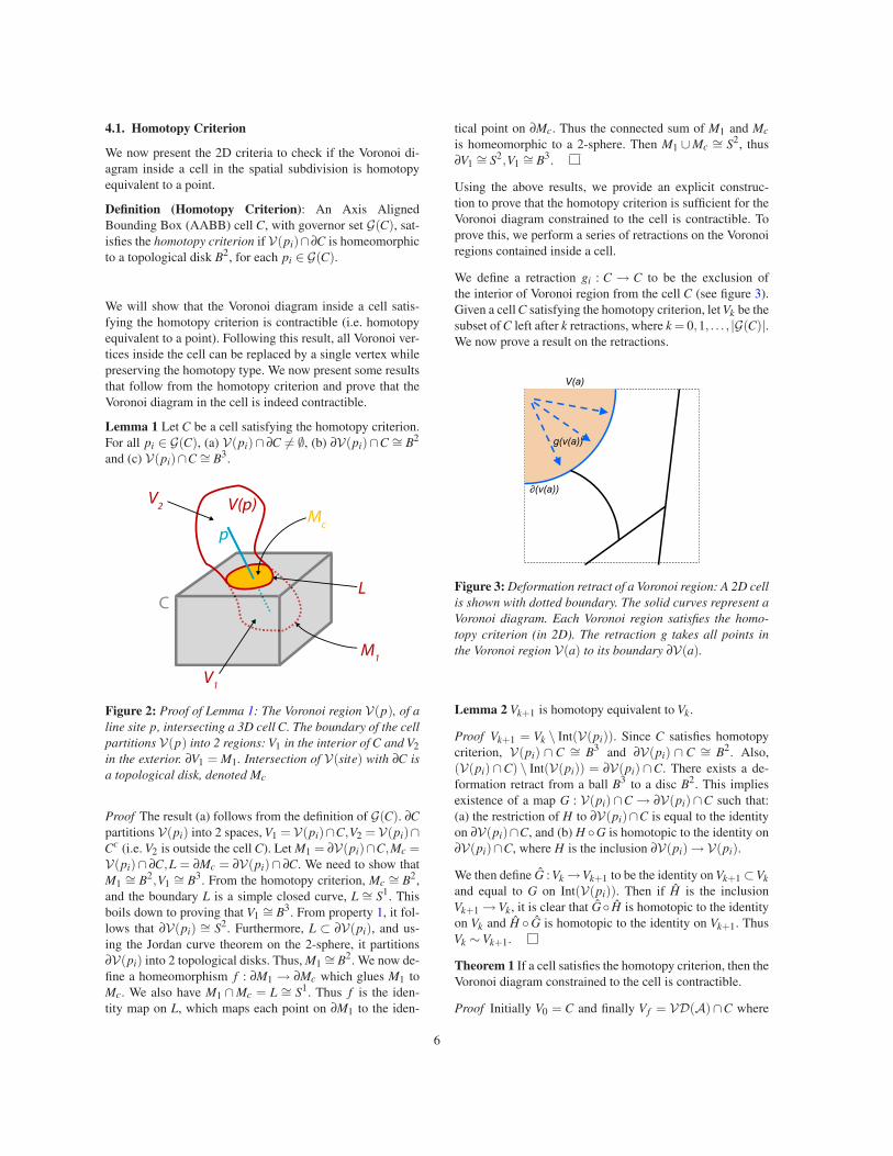
V(a)

g(v(a))

(v(a))

Figure 3: Deformation retract of a Voronoi region: A 2D cell

is shown with dotted boundary. The solid curves represent a

Voronoi diagram. Each Voronoi region satisfies the homo-

topy criterion (in 2D). The retraction g takes all points in

the Voronoi region V(a) to its boundary ∂V(a).

Lemma 2 Vk+1 is homotopy equivalent to Vk.

Proof Vk+1 = Vk \ Int(V(pi)). Since C satisfies homotopycriterion, V(pi) ∩ C ∼= B3 and ∂V(pi) ∩ C ∼= B2. Also,(V(pi)∩C) \ Int(V(pi)) = ∂V(pi)∩C. There exists a de-formation retract from a ball B3 to a disc B2. This impliesexistence of a map G : V(pi)∩C → ∂V(pi)∩C such that:(a) the restriction of H to ∂V(pi)∩C is equal to the identityon ∂V(pi)∩C, and (b) H ◦G is homotopic to the identity on∂V(pi)∩C, where H is the inclusion ∂V(pi) →V(pi).

We then define G : Vk →Vk+1 to be the identity on Vk+1 ⊂Vk

and equal to G on Int(V(pi)). Then if H is the inclusionVk+1 →Vk, it is clear that G◦ H is homotopic to the identityon Vk and H ◦ G is homotopic to the identity on Vk+1. ThusVk ∼Vk+1.

Theorem 1 If a cell satisfies the homotopy criterion, then theVoronoi diagram constrained to the cell is contractible.

Proof Initially V0 = C and finally V f = VD(A)∩C where

6

f = |G(C)|. From lemma 2, V0 and V f are homotopy equiv-alent. We know that the cell C is contractible. Thus V f iscontractible.

4.2. Completeness

In this section, we prove the completeness. To do this we usethe following theorem:

Theorem 2 For any point on the boundary of a Voronoi re-gion V(pi), there exists an open ball Br of strictly positiveradius r such that ∂V(pi)∩Br

∼= B2.

Proof We perform case analysis on the location of the point.

(a) The point lies in the interior of a Voronoi face. Each faceis a 2-manifold embedded in R

3. Then at each point on theface, there exists an open ball of finite radius such that inter-section of the ball with the face is 2-manifold - i.e. homeo-morphic to a disk.

(b) The point lies in the interior of a Voronoi edge. At aVoronoi edge, the Voronoi region is bounded by 2 Voronoifaces. Each bisector surface (i.e. a quadric surface) is dif-feomorphic to a disk. In a small neighborhood of the point,the arrangement of the Voronoi faces incident at the Voronoiedge is homeomorphic to the arrangement of a set of half-planes incident at an edge. The intersection of a half-planewith a sphere centered on the edge is a single curve seg-ment. Then the 2 curve segments, arising from the intersec-tion of the sphere and the two bounding Voronoi faces meetat exactly 2 points - the end points of the 2 curves. Thus theboundary of the intersection of Voronoi region boundary ata Voronoi edge and the boundary of ball (centered on edge)is a circle. Therefore, the intersection with the ball is a disk.

(c) The point lies on a Voronoi vertex. The proof for case(b) extends to this case. The boundary of a Voronoi region inthe neighborhood of a vertex consists of a finite number ofVoronoi faces meeting at Voronoi edges.

Theorem 2 implies that for any point on the Voronoi dia-gram VD(A), we can find a ball of a finite radius such thatthe intersection of the Voronoi regions with the ball satisfythe homotopy criterion. Thus the subdivision will terminateonce the current cell is contained inside such a ball.

5. Approximate Voronoi Diagram Computation

In this section, we present details of our algorithm. First wedescribe how we evaluate the homotopy criterion for eachVoronoi region in a given cell. Then we present our algo-rithm to compute the graph of the approximate Voronoi re-gion.

5.1. Homotopy Criterion Computation

Theorem 1 in Section 4 implies that this test reduces tochecking whether the intersection of the Voronoi diagram

with the boundary of a cell is homeomorphic to a disk. Thisis equivalent to determining if the intersection of the bound-ary of a Voronoi region with a cell is homeomorphic to a cir-cle. We compute the boundary of the Voronoi region alongeach face of the cell and compute the union over all faces.

The boundary of a Voronoi region consists of sheets, seamsand junctions. Each sheet is a subset of the bisector betweenthe carriers of two sites. Given a sheet fα and a cell face F ,a Voronoi face event is the intersection of fα and F and cor-responds to a conic curve on F in the general case. We com-pute an arrangement of the conics on the face [KCMh99].The intersection of the conic sections gives Voronoi edge

events [ER02], representing intersection of seams with a cellface. Along with each edge event, we store the set of gover-nors of the Voronoi edge. If the sheet is a plane tangential tocell face, we compute the intersection with the face vertices.In case the Voronoi edge event consists of infinite number ofpoints, we compute its intersection with the boundary of aface.

a b

d c

abg

abcd

ab

e

f

g

Figure 4: Homotopy criterion computation: We show a face

of a cell in the computation of approximate Voronoi diagram

of the L-shape. Each colored region represents the intersec-

tion of a Voronoi region with the face, and is labeled by its

governor. Each region is homeomorphic to a disc, hence sat-

isfies the homotopy criterion. The circles represent Voronoi

edge events: e.g. the point (abcd) represents intersection of

a degenerate Voronoi edge and the face. The bold conic seg-

ments represent the face events, representing boundary of the

Voronoi region of site a, computed by our tracing algorithm.

All intersections of conics do not provide the valid edgeevents. We compute the valid edge events based on the al-gorithm CellFaceVoronoiEdgeIntersection pre-sented in [ER02]. Given the set of edge events, we trace theconic segments between edge events sharing a common gov-ernor to obtain the Voronoi face events. A closed sequence offace events sharing a common governor provides the bound-ary of the Voronoi region of the site on the cell face. Twoedge events are connected by a face event if they share atleast two common governors (corresponding to the bisec-tor between the governors). In case there are multiple points

7

Figure 5: L-shape Model: The homotopy preserving ap-

proximate Voronoi diagram is computed for this model. The

edges of the approximate Voronoi diagram are shown in

blue. The vertices are highlighted with red. The orange re-

gion shows a zoomed in view of a degenerate vertex with 6seams incident on it.

sharing same 2 governor labels, we sort them according totheir parametric coordinates on the conic and connect the2 closest points. In the presence of degenerate seams, eachconic segment between two edge events may not represent avalid face event. Checking if a segment is a valid face eventis equivalent to determining if it lies on the boundary of theVoronoi region of a site pi. In order to perform this test,we enumerate all conic segments incident on an edge eventand trace along the conic segment which is closer to the pi

than to all other governors of the edge event. Finally, wejoin the face events at boundaries of adjacent faces to com-pute the intersection of the Voronoi region with the boundaryof the cell. A cell satisfies the homotopy criterion if all theVoronoi region boundaries on the cell boundary form onesimple closed loop.

5.2. Computing cell governors

The homotopy criterion needs to be satisfied for all sites thatbelong to the governor set of a cell. Here we present ourscheme to compute a set of governors of the cell. We use asequence of culling tests to prune the set of governors of acell. A site pi can be removed from the governor set of a cellC of diameter δ if:

1. Distance exclusion: There exists another governor p j ∈G(C) such that centroid of C is closer to p j and differencein distance is greater than δ.

2. Polytope exclusion: The domain polytope (a polytopebounding the Voronoi region of site pi) does not intersectC.

Figure 6: Cuboid Model with 2 equal dimensions: The edges

of the approximate Voronoi diagram are shown in blue. The

vertices are highlighted with red.

3. Bisector exclusion: There exists another governor p j ∈G(C) such the cell C is closer to p j and lies inside thedomain polytope of p j.

Each of these tests involves solving inequalities or a systemof linear equations [Cul00]. These tests provide a conser-vative estimate of the governors of a cell. The exact set ofgovernors of the faces of a cell is computed from the ar-rangement of Voronoi regions on the faces, as described insection 5.1. We now present a result that ensures computingthe arrangement on the boundary of a cell is sufficient forcomputing the cell governors.

Lemma 3 For an interior cell C, if V(p j)∩ Int(C) 6= ∅ thenV(p j)∩∂C 6= ∅.

The proof follows trivially from the facts that the Voronoi re-gions are connected (topological balls) and contain the site.A consequence of Lemma 3 is that it suffices to check theboundary of a cell to compute governors of an interior cell.For boundary cells, we impose further restrictions on thegovernor set of the cell to check if each Voronoi region in-tersects the cell boundary.

Boundary cell criterion: Given a boundary cell C, with aset of sites X intersecting C, C satisfies the boundary cellcriterion if:

1. X contains at most one point site pp, and X \{pi} con-tains sites incident on the point pi.

2. The governor set G(C) is a subset of X .

These two conditions ensure that each non point site in thegovernor set G(C) intersects the boundary of the cell - thustheir Voronoi regions must intersect the boundary of the cell.For each point site, its Voronoi region constrained to the cellis given by intersection of its domain polytope and the cell,thus its Voronoi region must intersect the cell boundary if itsdomain polytope is non-empty. Condition (1) can be triviallytested. We conservatively test for condition (2) by checking

8

if the conservative governor set does not include any sitesfrom A\X .

5.3. Approximate Voronoi Diagram Computation

In this section we provide our algorithm for computing a ho-motopy preserving approximate Voronoi diagram. We firstcompute a homotopy preserving approximate Voronoi graphusing spatial subdivision. The steps are given as follows:

1. Compute a discrete distance field on uniform grid at somefixed resolution.

2. Compute the governor set of each cell using exclusiontests presented in Section 5.2.

3. Check if a cell satisfies the homotopy criterion. In addi-tion, check if each boundary cell satisfies the boundarycriterion. If either of the criteria are not met, subdivideand update the governor sets of the children cells.

4. If a cell satisfies the homotopy and boundary criteria, in-sert a subgraph node inside the cell. Connect the node tothe edge events on the boundary of the cell.

This algorithm provides us with a homotopy preserving ap-proximate Voronoi graph. To extract the homotopy preserv-ing approximate Voronoi diagram, we further refine it to de-tect unique vertex nodes and edge nodes. We use a resultfrom [ER02] to detect Voronoi vertices: If the number of in-tersection points of a Voronoi edge eα and ∂C is odd, thenthere exists a Voronoi vertex in C. We subdivide a leaf cellif it contains more than two edge events with same governorset. If a cell has exactly two edge events with same gover-nor set, we remove the subgraph node and directly connectthe two edge events with a subset of the Voronoi edge. Therefined approximate Voronoi graph consists of nodes of typeVoronoi vertex and subgraph and edge nodes connecting thevertex and subgraph nodes. We follow a loop of Voronoiedge events joined by the same face event on the boundaryof a cell to extract the Voronoi faces.

6. Implementation and Results

In this section, we briefly describe our implementation andhighlight its performance on different benchmarks. We haveimplemented the system in C++, and use OpenGL to displaythe results. The timings reported in this paper were taken ona 2.4Ghz Opteron PC with 1GB of memory. The discretedistance field and spatial grid is computed efficiently usinggraphics hardware [SGGM06]. The resolution of the uni-form grid was chosen to be half of the length of the smallestedge of the polyhedron to ensure satisfiability of Condition(1) of the boundary criterion.

We have tested our algorithm on a set of examples from sim-ple geometry with known degenerate configurations to morecomplex models consisting of thousands of sites. Figure 5shows an L-bracket with symmetric cubical sections. The

bottom half contains degenerate seams and junctions. Fig-ure 7) shows a spoon model with 254 sites. Figure 8) showsa flattened chisel model with a radial axis of symmetry andrandom perturbations added to the handle. This benchmarkis particularly difficult to handle with many several degen-erate configurations near the axis of the handle. As a result,there is a large governor set for many cells.

Figure 7: Spoon Model: The model has 254 sites, including

84 triangle sites, 126 edge sites, and 44 vertex sites. The

computation for homotopy preserving approximate Voronoi

diagram took 1.7s for this model. The edges and vertices of

the approximate Voronoi graph are highlighted in blue and

red respectively.

Figure 8: Chisel Model: The model has 1,797 sites, includ-

ing 632 triangle sites, 847 edge sites, and 318 vertex sites.

It has many degenerate configurations near the axis of the

handle. Two views of the approximate Voronoi graph are

shown in the bottom. The computation for homotopy pre-

serving approximate Voronoi diagram took 130.3s for this

model. The edges and vertices of the approximate Voronoi

graph are highlighted in blue and red, respectively.

6.1. Homotopy Preserving MAT Approximation

We have applied our homotopy preserving Voronoi diagramcomputation algorithm to compute a homotopy preservingmedial axis approximation of 3D polyhedrons [SFM05]. Inpractice, this simplification tends to remove unstable fea-tures of Blum’s medial axis, while preserving the topolog-ical structure. In particular, we can guarantee that the ap-proximate medial axis is homotopy equivalent to the orig-inal shape. The approximate medial axis is extracted from

9

approximate Voronoi diagram by removing Voronoi faceswith a governor set such that one governor is a subset ofthe closure of the other. The elements of the medial axis areremoved using a stability measure based on the separationangle formed by connecting a point on the medial axis to itsgovernors. Some examples of the computed homotopy pre-serving approximate medial axis are shown in figures 9- 10.

(a) Model (b) Approximate MAT

Figure 9: Knot Model (2.5k polygons). The homotopy pre-

serving Voronoi diagram is used to compute a homotopy

preserving approximate medial axis (shown in green). The

sheets consist of thin and long faces. The Voronoi diagram

computation took 5.2s.

7. Discussion

In this section we perform an analysis of the individualstages of our algorithm and compare it with prior techniques.

7.1. Analysis and Comparisons

The total running time of the subdivision algorithm is de-pendent on the depth of the subdivision performed and therelative configuration of the Voronoi faces. In this section,we provide time bounds on the computation cost per cell,specifically the cost of computing the homotopy criterion.Let the size of governor set of a cell be k. Then the numberof intersection points is bounded by O(k2). Each intersection

Figure 10: Ridged Rod (5k polygons), The model has ridges

near the surface, which leads to many unstable features in

the medial axis. The sheets of the approximate medial axis

are shown in (b). The Voronoi diagram computation took

211s.

point is checked against remaining O(k) governors to deter-mine if it is a valid edge event. Given the set of edge events,they are sorted by their governor labels in O(k2 logk2) time.Next the algorithm used to trace the Voronoi edges in a singleregion boundary performs O(1) computations at each edgeevent. Thus the total cost of computing the edge events andtracing the all Voronoi region boundaries on a cell is at mostO(k3). Typically, the number of governors per cell is small,but in the worst case it can be k = O(N), N = number of en-tities on the boundary) for degeneration configurations. Theboundary criterion can be computed in O(k) time.

Comparison: We compare our algorithm to prior ap-proaches for computing the Voronoi diagram of polyhedralmodels.

The seam curve tracing methods [CKM04, SPB96, RT95]compute the exact Voronoi diagram. In practice, they cancompute a topologically correct Voronoi diagram, but theyrequire use of exact arithmetic to solve a system of tri-variatenon linear equations. Furthermore, they are prone to degen-erate configurations. As a result, these approaches may notscale well to large models.

Our work is most similar to work on computing an approx-imate Voronoi diagram using spatial subdivisionr. The workof [VO98, BCMS05, SS06] does not provide any topologi-cal guarantees on the computed approximate Voronoi dia-gram - instead the subdivision is carried out to a predefinedlevel. The work of Etzion and Rappoport [ER02] providesa topologically valid Voronoi graph for cells of size greaterthan some predefined constant ε. In general, it is not easyto select a good value of ε for large models. For degener-ate and near-degenerate configurations, they compute an ap-proximate Voronoi graph, with no topological guarantees. Incase of large cells, their approach computes an approxima-tion that is homeomorphic to the exact Voronoi diagram onlyfor non-degenerate configurations. Moreover, they requirethat the cells are subdivided till the number of governors ofa cell is small (typically 4− 6, except for special cases). Asa result, their approach can be rather conservative.

In comparison, our algorithm provides a less strict topolog-ical guarantee on the output. We ensure homotopy equiva-lence between the exact Voronoi diagram and our approxi-mation, even in the presence of degenerate and near degen-erate configurations. We exploit the fact that in the neigh-borhood of a near-degenerate configuration, the Voronoi di-agram is homotopy equivalent to a point and this propertysimplifies the overall computation. The homotopy criterion,introduced in Section 4.1, also checks for this condition in acell containing a degenerate configuration. Furthermore, thehomotopy criterion allows for early termination during sub-division, even if a call has a large number of governors. Thisresults in fewer levels of subdivision. In practice, the size ofleaf nodes in the subdivision is of similar scale as the inputgeometry.

10

7.2. Limitations

Our algorithm has a few limitations. The approximateVoronoi diagram computed by our algorithm is not home-omorphic to the exact Voronoi diagram. Since it is based onspatial subdivision, the cost of computation and the com-plexity of the approximate Voronoi diagram varies based onthe configuration the subdivision grid. In particular, one mayencounter degenerate configurations in which the intersec-tion of the Voronoi regions with the boundary of the cellmay be a single point (i.e. a tangential intersection), and suchcases cannot be easily resolved with only subdivisions. Webelieve a subdivision scheme which allows for perturbationof the cell faces may be able to alleviate this problem.

8. Conclusions and Future Work

We have presented an approach to compute a homotopy pre-serving approximate Voronoi diagram of a 3D polyhedron.Homotopy equivalence is a weaker topological guaranteecompared to homeomorphism, however it captures all thetopological features of the shape. Our algorithm is basedon an adaptive spatial subdivision, and guarantees that theVoronoi diagram in each cell is homotopy equivalent to apoint. The topological tests are performed by computing thearrangement of 2D conic sections.

Hence our algorithm is simpler than exact 3D Voronoi dia-gram computation and can handle near-degenerate configu-rations of the Voronoi diagram. We have highlighted its per-formance on many benchmarks and also used it to computea homotopy preserving medial axis approximation.

There are many avenues for future work. The approximatehomotopy preserving Voronoi diagram can have a compli-cated structure for large models. We would like to study var-ious methods for simplifying this structure and apply it todifferent applications like motion planning, feature identi-fication and shape analysis. Furthermore, we would like toevaluate the accuracy of those simplification schemes. Wewould also like to combine our algorithm to other subdivi-sion schemes such as kd-trees, which offer a better choice ofpartitioning planes.

References

[ABE04] ATTALI D., BOISSONAT J.-D., EDELSBRUN-NER H.: Stability and computation of the medialaxis. In Mathematical Foundations of Scientific Visualiza-

tion, Computer Graphics, and Massive Data Exploration.Springer-Verlag, 2004.

[ACK01] AMENTA N., CHOI S., KOLLURI R. K.: Thepower crust. In Proc. ACM Symposium on Solid Modeling

and Applications (2001), pp. 249–260.

[AK96] AURENHAMMER F., KLEIN R.: Voronoi Dia-

grams. Tech. Rep. 198, Department of Computer Science,FernUniversität Hagen, Germany, 1996.

[AK00] AURENHAMMER F., KLEIN R.: Voronoi dia-grams. In Handbook of Computational Geometry, SackJ.-R., Urrutia J., (Eds.). Elsevier Science Publishers B.V.North-Holland, Amsterdam, 2000, pp. 201–290.

[Aur91] AURENHAMMER F.: Voronoi diagrams: A surveyof a fundamental geometric data structure. ACM Comput.

Surv. 23, 3 (Sept. 1991), 345–405.

[BBGS99] BLANDING R., BROOKING C., GANTER M.,STORTI D.: A skeletal-based solid editor. In Proc. ACM

Symposium on Solid Modeling and Applications (1999),pp. 141–150.

[BCMS05] BOADA I., COLL N., MADERN N., SELL-ARES J. A.: Approximations of 3D generalized voronoidiagrams. In Proc. 21st European Workshop on Compu-

tational Geometry (2005), pp. 163–166.

[Be05] BERBERICH E., ET AL.: Exacus: Efficient and ex-act algorithms for curves and surfaces. Proc. of the 13th

European Symposium on Algorithms (2005).

[Boi86] BOISSONNAT J.-D.: Automatic solid modeler forrobotics applications. In Robotics Research: Third Inter-

national Symposium. MIT Press Series in Artificial Intel-

ligence. (Cambridge, MA, 1986), MIT Press, pp. 65–72.

[BPA01] BONNASSIE A., PEYRIN F., ATTALI D.: Shapedescription of three-dimensional images based on medialaxis. In 10th International Conference on Image Process-

ing (ICIP) (2001), pp. 931–934.

[CKM04] CULVER T., KEYSER J., MANOCHA D.: Exactcomputation of a medial axis of a polyhedron. Computer

Aided Geometric Design 21, 1 (2004), 65–98.

[CL04] CHAZAL F., LIEUTIER A.: Stability and homo-topy of a subset of the medial axis. In Proc. ACM Sympo-

sium on Solid Modeling and Applications (2004).

[CS04] CHAZAL F., SOUFFLET R.: Stability and finite-ness properties of medial axis and skeleton. Journal of

Control and Dynamical Systems 10, 2 (2004), 149–170.

[Cul00] CULVER T.: Accurate Computation of the Medial

Axis of a Polyhedron. PhD thesis, Department of Com-puter Science, University of North Carolina at ChapelHill, 2000.

[CZ06] CAO H.-D., ZHU X.-P.: A complete proof of thepoincaré and geometrization conjectures of the Hamilton-Perelman theory of the Ricci flow. Asian Journal of Math-

ematics 10, 2 (06 2006), 165 – 498.

[Den03] DENNY M.: Solving geometric optimizationproblems using graphics hardware. In Proc. of Euro-

graphics (2003).

[DZ02] DEY T. K., ZHAO W.: Approximating the me-dial axis from the Voronoi diagram with a convergenceguarantee. In European Symposium on Algorithms (2002),pp. 387–398.

[ER02] ETZION M., RAPPOPORT A.: Computing

11

Voronoi skeletons of a 3-d polyhedron by space subdivi-sion. Computational Geometry: Theory and Applications

21, 3 (March 2002), 87–120.

[FGLM01] FOSKEY M., GARBER M., LIN M.,MANOCHA D.: A voronoi-based hybrid planner.Proc. of IEEE/RSJ Int. Conf. on Intelligent Robots and

Systems (2001).

[HCK∗99] HOFF K., CULVER T., KEYSER J., LIN M.,MANOCHA D.: Fast computation of generalized voronoidiagrams using graphics hardware. Proceedings of ACM

SIGGRAPH 1999 (1999), 277–286.

[Hel01] HELD M.: Vroni: An engineering approach to thereliable and efficient computation of Voronoi diagrams ofpoints and line segments. Computational Geometry: The-

ory and Applications 18 (2001), 95–123.

[KCMh99] KEYSER J., CULVER T., MANOCHA D.,HNAN S. K.: MAPC: A library for efficient and exactmanipulation of alge braic points and curves. In Proc.

15th Annual ACM Symposium on Computational Geome-

try (1999), pp. 360–369.

[Lie03] LIEUTIER A.: Any open bounded subset of Rn

has the same homotopy type than its medial axis. InProc. ACM Symposium on Solid Modeling and Applica-

tions (2003), pp. 65–75.

[LM03] LIN M., MANOCHA D.: Collision and proxim-ity queries. In Handbook of Discrete and Computational

Geometry (2003).

[Mil93] MILENKOVIC V.: Robust construction of theVoronoi diagram of a polyhedron. In Proc. 5th Canad.

Conf. Comput. Geom. (1993), pp. 473–478.

[PG90] PATRIKALAKIS N. M., GÜRSOY H. N.: Shape in-terrogation by medial axis transform. In Proc. 16th ASME

Design Automation Conference (Sept. 1990).

[PSS∗03] PIZER S. M., SIDDIQI K., SZEKELY G., DA-MON J. M., ZUCKER S. W.: Multiscale medial loci andtheir properties. International Journal of Computer Vision

55 (2003), 155–179.

[RT95] REDDY J., TURKIYYAH G.: Computation of3D skeletons using a generalized Delaunay triangulationtechnique. Computer-Aided Design 27 (1995), 677–694.

[SA95] SHARIR M., AGARWAL P. K.: Davenport-

Schinzel Sequences and Their Geometric Applications.Cambridge University Press, New York, 1995.

[SERB98] SHEFFER A., ETZION M., RAPPOPORT A.,BERCOVIER M.: Hexahedral mesh generation using theembedded voronoi graph. 7th International Meshing

Roundtable (1998), 347–364.

[SFM05] SUD A., FOSKEY M., MANOCHA D.: Homo-topy preserving medial axis simplification. In Proc. ACM

Symposium on Solid and Physical Modeling (2005).

[SGG∗06] SUD A., GOVINDARAJU N., GAYLE R.,

KABUL I., MANOCHA D.: Fast proximity computa-tion among deformable models using discrete voronoi di-agrams. ACM Trans. Graph. (Proc ACM SIGGRAPH) 25,3 (2006), 1144–1153.

[SGGM06] SUD A., GOVINDARAJU N., GAYLE R.,MANOCHA D.: Interactive 3d distance field computationusing linear factorization. In Proc. ACM Symposium on

Interactive 3D Graphics and Games (2006), pp. 117–124.

[She95] SHERBROOKE E. C.: 3-D Shape Interrogation

by Medial Axis Transform. Ph.D. thesis, Dept. Ocean En-gineering, Massachusetts Institute of Technology, Cam-bridge, Massachusetts, 1995.

[SOM04] SUD A., OTADUY M. A., MANOCHA D.: DiFi:Fast 3D distance field computation using graphics hard-ware. Computer Graphics Forum (Proc. Eurographics)

23, 3 (2004), 557–566.

[Spa89] SPANIER E. H.: Algebraic Topology. Springer,1989.

[SPB96] SHERBROOKE E. C., PATRIKALAKIS N. M.,BRISSON E.: An algorithm for the medial axis transformof 3d polyhedral solids. IEEE Trans. Visualizat. Comput.

Graph. 2, 1 (Mar. 1996), 45–61.

[SS06] STOLPNER S., SIDDIQUI K.: Revealing signifi-cant medial structure in polyhedral meshes. In Third In-

ternational Symposium on 3D Data Processing, Visual-

ization and Transmission (2006).

[Sug92] SUGIHARA K.: Algorithms for computingVoronoi diagrams. In Spatial Tesselations: Concepts and

Applications of Voronoi Diagrams, Okabe A., Boots B.,Sugihara K., (Eds.). John Wiley & Sons, Chichester, UK,1992.

[Sur03] SURESH K.: Automating the CAD/CAE dimen-sional reduction process. In Proc. ACM Symposium on

Solid Modeling and Applications (2003), pp. 76–85.

[TH03] TAM R., HEIDRICH W.: Shape simplificationbased on the medial axis transform. IEEE Visualization

(2003).

[TT97] TEICHMANN M., TELLER S.: Polygonal Approxi-

mation of Voronoi Diagrams of a Set of Triangles in Three

Dimensions. Tech. Rep. 766, Laboratory of ComputerScience, MIT, 1997.

[VO98] VLEUGELS J., OVERMARS M. H.: Approximat-ing Voronoi diagrams of convex sites in any dimension.International Journal of Computational Geometry and

Applications 8 (1998), 201–222.

[Wol92] WOLTER F. E.: Cut Locus and Medial Axis in

Global Shape Interrogation and Representation. Tech.Rep. 92-2, MIT, Dept. Ocean Engg., Design Lab, Cam-bridge, MA 02139, USA, Jan. 1992.

12