Homotopy-Preserving Medial Axis Simplification

Avneesh Sud∗

Department of Computer Science

Mark Foskey†

Department of Radiation Oncology

Dinesh Manocha‡

Department of Computer Science

University of North Carolina at Chapel Hill

Abstract

We present a novel algorithm to compute a simplified medialaxis of a polyhedron. Our simplification algorithm tends toremove unstable features of Blum’s medial axis. Moreover,our algorithm preserves the topological structure of the orig-inal medial axis and ensures that the simplified medial axishas the same homotopy type as Blum’s medial axis. We usethe separation angle formed by connecting a point on themedial axis to closest points on the boundary as a measureof the stability of the medial axis at the point. The medialaxis is decomposed into its parts that are the sheets, seamsand junctions. We present a stability measure of each partof the medial axis based on separation angles and exam-ine the relation between the stability measures of adjacentparts. Our simplification algorithm uses iterative pruningof the parts based on efficient local tests. We have appliedthe algorithm to compute a simplified medial axis of com-plex models with tens of thousands of triangles and complextopologies.

Keywords: Medial Axis, Voronoi diagram, homotopy,simplification, separation angle

1 Introduction

The medial axis of a geometric object is the set of interiorpoints that have at least two closest points on the boundaryof the object. The medial axis can also be defined as the setof centers of at least twice tangent maximal balls containedinside the object. This formulation was originally proposedby Blum [1967] and many authors have proposed extensionsto this formulation. Given a 3D solid, its medial axis con-sists of a union of surfaces that provide useful informationabout its shape and topology. The medial axis transform(MAT) consists of all the medial axis points and the distanceto the boundary from each medial point. MAT has appli-cations in image analysis and computer vision [Pizer et al.2003], solid modeling [Blanding et al. 1999], mesh genera-tion and finite element analysis [Sheffer et al. 1998; Suresh2003], shape simplification [Tam and Heidrich 2003], motionplanning [Foskey et al. 2001], etc.

Given a 3D solid, there are two main issues in the compu-tation of MAT: algebraic complexity and instability. The

∗e-mail: sud@cs.unc.edu†e-mail: mark foskey@unc.edu‡e-mail: dm@cs.unc.edu

algebraic complexity arises from the fact that the sheets,seams and junctions of a medial axis are high degree alge-braic primitives and it is hard to compute the exact MATreliably for complex models. Many techniques have beenproposed in the literature to approximate the medial axis.At a broad level these techniques either compute the Voronoidiagram of a point sample on the boundary of the solid orevaluate the distance field of the primitives on a spatial gridfollowed by isosurface extraction.

The instability refers to the property that small modifica-tions to the boundary of the solid can induce large modi-fications in its medial axis. Different algorithms have beenproposed to compute a stable subset of the medial axis basedon different geometric criteria. However, current algorithmsare either limited to point datasets or may not preserve thetopology of the medial axis.

Main Results: We present a novel algorithm to computea homotopy preserving simplification of the medial axis ofpolyhedral models. Our algorithm computes a polygonalapproximation that has the same homotopy type as Blummedial axis and thereby preserves its topological structure.Our simplification algorithm is based on the separation angle[Amenta et al. 2001; Dey and Zhao 2002; Dimitrov et al.2003] and simplified medial axis [Foskey et al. 2003] andattempts to remove features on the medial axis for whichthe separation angle is below a certain threshold.

We initially compute a connectivity graph that representsthe connectivity of the original medial axis. We present aniterative algorithm that removes sheets from the medial axisbased on the separation angle criterion without changing thehomotopy type of the medial structure. We maintain a pri-ority queue of the sheets ordered by the separation angleand compute a simplification of the medial axis by remov-ing sheets from the queue that correspond to the unstableparts. We give rigorous guarantees on the homotopy of thesimplified medial axis. Our simplification algorithm can alsobe applied to other medial axis formulations as long as weare given an approximation with correct homotopy.

Some of the novel results of our work include:

� A homotopy preserving medial axis simplification algo-rithm applicable to continuous solid representations.

� Relationship between the stability of medial axis junc-tions and seams to stability of incident sheets usingseparation angles.

� Algorithm to compute the stability of a medial axissheet using discrete sampling.

We have implemented the algorithm on a PC with 2.4GHzPentium IV processor and applied it to complex CAD modelsconsisting of tens of thousands of triangles. Our algorithmis able to simplify the medial axis of these models whilepreserving the homotopy in a few seconds.

As compared to prior algorithms for medial axis simplifica-tion, our algorithm offers the following advantages:

�Polyhedral Models: Our simplification algorithm isapplicable to models with continuous piecewise linearboundaries, possibly with internal voids.

�Complex Models: Our algorithm is able to handlecomplex models with a high number of boundary prim-itives and complex topologies.

�Homotopy Preservation: The simplified medial axishas the same topological structural as the original me-dial axis. These properties are important for shapeanalysis, motion planning and mesh generation.

�Efficiency: Our simplification is based on iterativepruning of the connectivity graph and is computed us-ing local operations.

Organization: The rest of the paper is organized in thefollowing manner. We give a brief overview of previous workin Section 2. We introduce our notation and present back-ground material in Section 3. We present the formulationof a topology preserving simplified medial axis in Section4 and describe our algorithm in Section 5. We prove thecorrectness of algorithm in Section 6. We describe its im-plementation in Section 7 and highlight its performance ondifferent benchmarks. We analyze its performance and com-pare it with other approaches in Section 8.

2 Related Work

In this section we give a brief overview of prior work on me-dial axis computation as well as medial axis simplification.We make this separation for convenience, but it is importantto realize that the two are often integrated in practice.

2.1 Medial Axis Computation

In this section we focus on methods to generate a (possiblyapproximate) medial axis of a figure or object. The algo-rithms are categorized based on different model representa-tions.

Image datasets. The problem of MAT computation of apoint dataset has been extensively studied in computer vi-sion and image processing. In two and three dimensions,approximations to the medial axis have been computed us-ing thinning algorithms [Lam et al. 1992; Zhang and Wang1993]. Many algorithms based on partial differential equa-tions of front propagation have also been proposed [Kimmelet al. 1995; Siddiqi et al. 1997]. Pizer et al. [2003] havegenerated structures related to the medial axis using filterswhich yield high values for points near the medial axis of anobject.

Boundary point samplings. Algorithms for computingthe medial axis of an object from a sample of points onthe boundary typically begin by constructing a Voronoi di-agram of the point set, after which they use various criteriato prune faces [Amenta et al. 2001; Dey and Zhao 2002; Nafet al. 1996; Ogniewicz and Kubler 1995; Sheehy et al. 1995;Shaham et al. 2004].

Polyhedral Models. Many MAT computation algorithmshave been proposed for polyhedral models based on 3Dtracing of the seam curves [Milenkovic 1993; Reddy andTurkiyyah 1995; Sherbrooke et al. 1996]. These algorithms

solve a system of algebraic equations to compute the junc-tion points and the seam curves. Culver et al. [1999] usedexact arithmetic to compute the MAT accurately. Etzionand Rappoport [2002] used spatial subdivision techniques todetermine connectivity of the MAT and only can guaranteecorrectness up to a certain resolution. All these algorithmshave been applied to polyhedral models with a few hundredtriangles. Foskey et al. [2003] used graphics hardware togenerate an image-space representation of the gradient ofthe distance field to the boundary, which can be analyzedto find the medial axis. The gradient field in their methodis actually the same as the velocity field of the propagat-ing front in the methods of Siddiqi et al. [2002] mentionedabove. Du and Qin [2004] also computed an approximationof the medial axis using diffusion partial differential equa-tions solved at a discrete sample of boundary points. Yanget al. [2004] generated sample points on the boundaries ofmaximal spheres, and apply a separation angle criterion (seebelow) to select the points approximately on the medial axis.

2.2 Medial Axis Simplification

In this section we give a brief overview of medial axis sim-plification algorithms. The instability of the medial axis,and its resulting complexity for objects with boundaries ex-hibiting fine detail, has been known for some time (see forinstance, Blum and Nagel [1978]). A number of methodsfor simplifying the medial axis have been proposed. Pizer etal. [2003] have presented an extensive survey of methods forapproximating and simplifying the medial axis.

A well known criterion for medial axis simplification is basedon the object angle [Dimitrov et al. 2003]. The separationangle is twice the object angle at any point on the medialaxis. The underlying methods involve computing subsetsfor which the object angle is above a certain threshold. Ma-landain and Fernandez-Vidal [1998] traced the idea, in vary-ing forms, back to Meyer [1979] and Kruse [1991]. Our sim-plification algorithm also uses this criterion.

Siddiqi et al. [2002] formulated the detection of gradientdiscontinuities in terms of the average gradient flux into aneighborhood, which has been shown to be closely relatedto the object angle [Dimitrov et al. 2003]. Malandain andFernandez-Vidal [1998] used a criterion combining the ob-ject angle and the distance between the two points nearestto the medial axis point. Foskey et al. [2003] detected gradi-ent discontinuities across adjacent voxels by comparing thedirections of neighboring vectors.

Another class of approaches are based on using a point sam-pling of the boundary. These algorithms approximate themedial axis by computing the Voronoi diagram of the setof points and eliminating some of the Voronoi faces usingdifferent criteria. Amenta et al. [2001] used the distance be-tween the two points nearest to the medial axis point as acriterion for medial axis simplification. Dey and Zhao [2002]combined a similar distance criterion with an object anglecriterion and observed that the two criteria together tendto eliminate spurious holes. Tam and Heidrich [Tam andHeidrich 2003] used a volume criterion to remove parts ofthe medial axis while preserving the topology. Leymarieand Kimia [2001] also began with surface point samples, buttheir algorithms are based on the differential equations offront propagation.

2.3 Topological and Smoothness Properties of MAT

Attali, Boissonat, and Edelsbrunner [Attali et al. 2004] havesurveyed different techniques that generate a stable and ho-motopy preserving medial structure. The homotopy rela-tionship between an object and its medial axis has beenproven in a particularly general form by Lieutier [2003], whoshowed that homotopy preservation holds for any boundedopen subset of R

n. Chazal and Soufflet [2004] presentedsmoothness constraints on the boundary of a solid, whichneed not be polyhedral, under which the medial axis obeyscertain stability and finiteness conditions. Chazal and Lieu-tier [2004] have also proven results about stability, and pre-sented a homotopy preserving medial axis simplification,however the approach has not been demonstrated on com-plex models. We discuss some of these simplification meth-ods in relation to our work in section 8.

3 Notation and Background

In this section, we introduce some of the terminology used inthis paper. We also give a brief overview of the θ-simplifiedmedial axis (θ-SMA).

3.1 Basic Terminology

The notations are summarized in table 1, and are formallydefined below. In this paper we will consider only polyhedralsolids, which we refer to as an object O. The solid O canhave internal voids. For a point x ∈ O, any point on theboundary of O that is at least as close to x as any otherwill be called a nearest neighbor of x, and the set of nearestneighbors will be called the neighbor set of x and denotedNS(x). With a distance function d(),

NS(x) = {y ∈ ∂O | d(x,y) = d(x, ∂O)}.

Then the medial axis of O, denotedM, is defined as the setof points inside O with at least two nearest neighbors.

The boundary of O can be decomposed disjointly into ver-tices, open edges, and open faces, which we refer to collec-tively as sites. Each nearest neighbor of x will be in exactly

Notation Meaning

X c Closure of a set XX Compliment of XX ◦ Interior of X∂X Boundary of X|X | Cardinality of XO Polyhedral solid in R

3

pi A face, edge or vertex site on ∂Oni(x) Normal to a site pi from a point xNS(x) Set of boundary points closest to x ∈ OGov(x) Set of boundary sites closest to x ∈ OM Medial axis of OF , fi Set of sheets of M, one sheet of ME , ei Set of seams of M, one seam of MV, vi Set of junctions of M, one junction of MR(fi) Set of rim curves of a sheet fi

S(fi) Set of seam curves of a sheet fi

Table 1: Notation used in the paper

one site, and we define the set of neighboring sites Gov(x)to be the set of sites containing a nearest neighbor of x:

Gov(x) = {pi | y ∈ pi for some y ∈ NS(x)}.

For each point x ∈M, the sites in the set Gov(x) are calledthe governors of the point x. Clearly, |Gov(x)| ≥ 2 for anypoint x on the medial axis.

3.2 Medial Axis Point Classification

We define a sheet set to be the set of all medial axis pointsgoverned by a specified pair of sites (or at least having thatpair among their governors), and we define a sheet to be aconnected component of a sheet set. The interior of a sheetis a smooth surface. A sheet may contain holes, because wedo not require that the boundary of O be connected or haveonly simply connected faces. A seam curve, or seam, is a con-nected component of the intersection of two or more sheets.The intersection of three or more seams is a junction. Thisdefinition corresponds approximately to those given in [Cul-ver et al. 1999] and [Sherbrooke et al. 1996]. Finally, for anysubsetM′ ofM, the intersection of a seam with the bound-ary will be a seam end. The intersection of a sheet withseam ends removed, and the boundary of M′ will be a rimset. An example of seam points, junction points, and rimpoints is given in figure 1. A similar classification of medialaxis points for any bounded set in R

3 is given in [Giblin andKimia 2000].

We make one special proviso about rims and seam ends. Ingeneral, including the case whenM′ =M, the boundary ofM′ will not be contained in M′. In this case, it is possiblethat two sheets that do not intersect will have boundariesthat do intersect. If this occurs, their rim curves and seamends will be treated as distinct combinatorial entities, sincethe goal is to reflect the connectivity properties of M, notits closure.

Figure 1: Medial axis point classification: (a) Classificationof the points on the medial axis (thin lines) of a simple poly-hedron (thick lines) (b) A subsetM′ ⊂M is shaded in gray.A rim point and a seam point on the boundary of the centralsheet are shown.

3.3 Homotopy Equivalence

One of the major goals of our work is to compute a simplifi-cation of the MAT that is homotopy equivalent to the exactMAT. The notion of homotopy equivalence between topolog-ical sets enforces a one-to-one correspondence between con-nected components, holes, tunnels or cavities and also the

way in which they are related. It has been shown by Lieu-tier [Lieutier 2003] that any bounded open subset X ⊆ R

n

is homotopy equivalent to its medial axis. Intuitively thisimplies that the medial axis and the shape are connected inthe same way.

Formally, two maps f : X → Y and g : X → Y are homotopicif there exists a continuous family of maps ht : X → Y, fort ∈ [0, 1], such that h0 = f and h1 = g. Thus, a homotopyis a deformation of one map to another. Two spaces X andY are homotopy equivalent if there exist continuous mapsf : X → Y and g : Y → X such that g ◦ f and f ◦ g arehomotopic to the identity maps on their respective spaces.As an example, f could be the inclusion of a circle into anannulus, and g could be radial projection of the annulus ontothe circle.

In situations such as this one, where f is an inclusion and f◦gis actually equal to the identity map, the homotopy equiva-lence is called a deformation retraction. See Spanier [1989]for details of these definitions. Our simplification algorithmalso performs a sequence of deformation retractions on theoriginal medial axis to generate a simplified medial axis withthe same homotopy type as the original.

3.4 θ-Simplified Medial Axis

Given a polyhedral model O and a medial axisM, the sepa-ration angle Θ(x) at each point x onM is the largest anglesubtended by a pair of nearest neighbor points on ∂O, andis given by

Θ(x) = maxyi,yj∈NS(x)

(∠yixyj)

Given an angle θ, the θ-simplified medial axis (θ-SMA) ofO, denoted by Mθ, is the set of points of M with separa-tion angle greater than θ [Foskey et al. 2003] (see figure 2).Foskey et al. [2003] discuss the convergence and stability

Figure 2: θ-Simplified Medial Axis,Mθ: (a) The medial axis(black) of a part of a polyhedron (blue) (b)Mθ for θ = π/2.

of Mθ and provide error bounds on the boundary recon-structed from Mθ. The speed of medial axis formation atpoint x is proportional to 1

sin Θ(x)[Pizer et al. 2003]. Parts

of the medial axis with a higher speed of formation are re-garded as more important [Blum 1967], and the separationangle Θ(x) has been used as a measure of the stability of themedial axis at the point x.

4 θ-Homotopy Medial Axis

In this section, we analyze the topological characteriza-tion of θ-SMA and present a formulation for computing a

homotopy-preserving simplified medial axis, the θ-homotopymedial axis. The problem with the θ-SMA is that it doesnot in general preserve the homotopy type of the medialaxis. The θ-SMA can be disconnected when the medial axisis connected, or have holes when the medial axis does not,and lack holes when the medial axis has them. An illus-tration of the failure of connectivity is shown in Figure 3.The other kinds of connectivity problems also arise because

Figure 3: The θ-Simplified Medial Axis, Mπ/3 is discon-nected even though the original object O is connected. Notethat the separation angle at x is less than π/3, while it ex-ceeds π/3 for the portions of the medial axis shown.

the angle criterion may discard topologically significant por-tions. The fundamental issue here is that homotopy typeis a global property, whereas the separation angle is a localmeasure.

Decreasing the θ threshold does not provide a guaranteedsolution to fix the problems. As illustrated in Figure 3, theproblem is associated with local minima of the separationangles, and such a local minimum can occur for any value ofθ. In any event, decreasing θ only increases the number ofunstable features of the θ-SMA.

Our goal is to compute a simplified medial axis that wouldallow significant simplification corresponding to large valuesof θ, while preserving the homotopy type of M. Clearlysuch a simplified medial axis has to be a superset of Mθ.However, we would like such an axis to be minimal in someregard in order to minimize the unstable parts. We nowformally present the desired subset of the medial axis. LetHθ denote the class of subsets of M which are supersets ofMθ and are homotopy equivalent to M.

Hθ = {X |X ⊆M,X ⊇Mθ,X 'M}

Define a set X ∈ Hθ to be irreducible if the removal of anysheet yields a set that either has a different homotopy type,or is no longer a superset of Mθ. That is,

M∗θ = {X |X ∈ Hθ, for all fi ∈ X , (X \ {fi}) /∈ Hθ}

We will refer to any irreducible set in Hθ as a θ-homotopymedial axis, or θ-HMA. We will typically denote a θ-HMAbyM∗

θ . The setM∗θ is not unique. A discussion about lack

of uniqueness is presented in section 8.

5 θ-Homotopy Medial Axis Computation

In this section we present an algorithm for computing a θ-HMAM∗

θ . We begin by computing a Voronoi diagram of thepolyhedron using spatial subdivision techniques presented

in [Sud and Manocha 2005]. Our approach is similar tothe subdivision algorithm of [Etzion and Rappoport 2002].A Voronoi graph is computed that represents the connec-tivity of the Voronoi diagram of the polyhedron. A nodein the graph corresponds to a Voronoi face, edge or vertexand an edge indicates an incidence relationship between twonodes. The algorithm computes an exact Voronoi graph ofthe polyhedron if the Voronoi diagram is not degenerate. Inpresence of degeneracies, it computes an ε-Voronoi graph,similar to [Etzion and Rappoport 2002]. However, in con-trast to this work, our algorithm subdivides a cell till thearrangement of Voronoi faces can be unambiguously deter-mined from a labeling of the governors at the corners ofthe cell. We use a simple subdivision criteria, and reducecomputation of intersections of conic sections on faces of acell. Furthermore, the algorithm can handle internal voidsin the polyhedron. Given the Voronoi graph, a sub-graphcorresponding to the medial axis M of the polyhedron iscomputed using the property of Lemma 12 in [Etzion andRappoport 2002]. The Voronoi faces, edges and vertices cor-respond to the medial axis sheets, seams and junctions re-spectively. We refer to this sub-graph, which captures theconnectivity of different elements of the medial axis M, asthe connectivity graph of M.

The diameter of a cell after the spatial subdivision givesa polygonal approximation to the geometric part of theVoronoi diagram. The approximation has bounded Haus-dorff error to the exact Voronoi diagram, like the ProximityStructure Diagram [Etzion and Rappoport 2002]. This geo-metric approximation is used to construct a polygonal meshapproximation of the θ-HMA consisting of axis aligned faces.

Given the exact medial axisM, our simplification algorithmis presented in Section 5.2 and it simplifies the medial axisby pruning sheets of the medial axis. We first define theseparation angle of a sheet fi to be the supremum of theseparation angles for all points interior to the sheet:

Θ(fi) = maxx∈f◦

i

(Θ(x)).

Θ(fi) gives a measure of the stability of the sheet fi. Weuse a conservative definition for the separation angle of thesheet to ensure that the simplified medial M∗

θ is a supersetof Mθ. Similarly we define the separation angle of a seamei as:

Θ(ei) = maxx∈e◦

i

(Θ(x)).

5.1 Sheet Separation Angle Computation

The Voronoi diagram computation algorithm computes apiecewise linear approximation of each sheet based on a dis-crete sampling introduced by spatial subdivision. In thissection, we address the problem of computing a boundedapproximation of the sheet separation angle Θ(fi). Eachsheet of the medial axis of a polyhedron is trimmed quadricsurface [Culver 2000]. Exact computation of the sheet sepa-ration angle involves computing the extreme value of a non-linear function on a quadric surface. Instead we present anefficient approach to compute a conservative upper bound onthe separation angle using spatial subdivision. The tightnessof the bound depends on the degree of subdivision.

Given a cell C and a sheet fi intersecting the cell, our goal isto compute the maximum separation angle for all points onthe sheet inside the cell. Let {p1, p2} be the two governors

of the sheet fi and c be the center of the cell C. We classifythe inputs into 2 cases:

1. The governors do not intersect the cell C, i.e. C ∩{p1, p2} = ∅

2. At least one of the governors intersects the cell C, i.e.C ∩ {p1, p2} 6= ∅.

Case 1: C ∩{p1, p2} = ∅. We simplify the problem to com-puting the maximum of the separation angles for all pointsinside the cell to the two governors. We compute the sepa-ration angle from the center c of the cell to each of the twogovernors and add conservative error bounds to get the max-imum separation angle. Let x be any point inside cell C. Letni(x) denote the normal vector from a point x to the sitespi, (i = 1, 2), and αi(x) represent the angle between ni(c)and ni(x). If ∆θi is an upper bound on αi(x) for all x ∈ C,then the maximum separation angle for sheet fi inside cellC is given by:

Θ(fi ∩ C) ≤ cos−1

(

n1(c) · n2(c)

|n1(c)||n2(c)|

)

+ ∆θ1 + ∆θ2

The computation of the error bounds ∆θi for each of thethree types of governors (point site, line site and trianglesite) is presented below:

Figure 4: Normal Cone to compute ∆θ for a point site

Point Site pi : p. The range of angles subtended by a pointsite to all points in the cell is given by a normal cone. Thenormal cone is the smallest cone enclosing the cell C with theapex at p and axis along ni(c) (see figure 4). Let ∆θi be thehalf opening angle of the cone. The angle αi(x) is maximizedwhen point x is one of the corner vertices vj (1 ≤ j ≤ 8) ofthe cell C. Thus, for the smallest cone enclosing the cell C,

∆θi = max1≤j≤8

[

cos−1

(

ni(vj) · ni(c)

|ni(vj)||ni(c)|

)]

, where ni(x) = p−x.

Line Site pi : p+λ(q−p). The range of angles subtended

Figure 5: Wedge to determine ∆θ for a line site

by a line to all the points in the cell is given by the smallestwedge enclosing the cell, with the top edge of the wedgebeing the line site (see figure 5). Let ∆θi be the half angleof the wedge. As in the point site case, the angle αi(x)is maximized when point x is one of the corner vertices vj

(1 ≤ j ≤ 8) of the cell C. Thus, for the smallest wedgeenclosing the cell C,

∆θi = max1≤j≤8

[

cos−1

(

ni(vj) · ni(c)

|ni(vj)||ni(c)|

)]

,

where ni(x) = p + λ(q− p)− x, λ =(x− p) · (q− p)

(q− p)2.

Triangle Site pi with face normal n. The shortest pathfrom any point to the triangle is perpendicular to the face.Thus ni(x) = n for all x, and ∆θi = 0.

Case 2 C ∩ {p1, p2} 6= ∅. If the two sites do not intersect(p1 ∩ p2 = ∅), then the bisector surface (and sheet fi) alsodo not intersect either site. In such a case we can subdividethe cell C into sub-cells {Ck} such that Ck ∩ {p1, p2} = ∅ ifC ∩ fi 6= ∅. The computation of the sheet separation angleis then reduced to Case 1.

If the two sites intersect (p1 ∩ p2 6= ∅), then the sheet corre-sponds to one of the non-generic cases of a bisector surface[Culver 2000], and the separation angle Θ(fi) can be deter-mined exactly from the pairs of governors. The case of twopoint governors case never occurs, we examine each of theother 5 pairs of governors individually.

Point-Triangle The bisector surface is a redundant line,and never occurs on the medial axis [Culver 2000].

Point-Line The bisector surface is a plane through the pointand perpendicular to the line, Θ(fi) = 0

Line-Line The bisector surface is an orthogonal plane pair,Θ(fi) = angle between the two lines.

Line-Triangle The bisector surface is a right circular cone,or a plane if the line is incident on the triangle. In first

case, the separation angle Θ(fi) = π/2− cos−1(l · n), where

l and n are unit normals along the line and to the trianglerespectively. In the second case, Θ(fi) = 0.

Triangle-Triangle The bisector surface is an orthogonalplane pair, and the separation angle is given by Θ(fi) =cos−1(n1 · n2), where n1, n2 are unit normals to the twotriangles.

5.2 Simplification Algorithm

We now present our medial axis simplification algorithm.We treat the medial axis M as an abstract 2-dimensionalcomplex consisting of faces, edges, and vertices. Initially,edges correspond either to the seam curves, which lie be-tween sheets, or rim curves, which lie on the boundary.

The key idea in our algorithm is a simple criterion for deter-mining whether a sheet can be removed without changingthe homotopy type of the medial structure. We call suchsheets frontier sheets (Figure 6). We will describe this crite-rion below, but first give an overview of how it is used in thealgorithm. We maintain a set Q of all frontier sheets. Wesuccessively remove sheets from this set until it is empty. Aseach sheet is removed from Q, it is also removed from the

Figure 6: Classification of sheets for iterative pruning: Thesheets colored gray are frontier sheets, and can be removedwithout changing the homotopy type. For the ‘loop’ sheets therim set is not connected and they will never become frontiersheets. The ‘interior’ sheet has an empty rim set, howeverit may become a frontier sheet after removal of one of itsadjacent sheets.

medial structure if its separation angle is no greater than θ.Removal of a sheet from the structure can affect whether itsneighbors are frontier sheets, and so each time we remove asheet we check each neighbor of that sheet to see if it needseither to be added or removed.

A sheet fi is defined to be a frontier sheet provided that itsset of rim points R(fi) and its set of seam points S(fi) areboth connected and nonempty. The set Q is defined as:

Q = {fi | R(fi) 6= ∅,R(fi) is connected,

S(fi) 6= ∅,S(fi) is connected}. (1)

In Section 6.2 we will prove that the frontier sheets are pre-cisely those sheets which may be removed without changingthe homotopy type. We present an intuitive justificationfor that claim here. If the rim set and seam set are bothconnected then each set is a single curve, and removing thesheet is equivalent to retracting the sheet onto its seam setvia a homotopy (see Figure 7(a)). On the other hand, if

Figure 7: Sheet pruning: (a) The cyan sheet is a valid fron-tier sheet, and has a deformation retract to its seam set. (b)The cyan sheet is not a frontier sheet. (c) Removing thesheet makes the two adjacent sheets disconnected.

the rim set is disconnected or empty, removing the sheetremoves a path between two points on different seam com-ponents and hence does not preserve the homotopy type (seeFigures 7(b),(c)). Note that, when we remove a sheet, weremove its interior and its rim set, but not its seam set.

We noted earlier that removing a sheet can cause othersheets either to lose or gain frontier status, and we can nowexplain why this is true. A sheet with an empty rim set cangain a rim edge if one of its neighboring sheets is removed,and thereby become a frontier sheet. Conversely, a sheetwith a single seam component can find that its seam set isbroken into two components if an adjacent sheet is removed.

Algorithm 1 simplifiesM based on removal of frontier sheets.Let the resulting medial subset after the jth iteration beMj , and let the corresponding frontier set be Qj . The fron-tier set is maintained as a priority queue, the priority deter-

Input: Initial (Blum) medial axis M0, angle θOutput: Final medial subset Mf

Label all sheets in M as unmarked1

Initialize Q0, j ← 02

repeat3

fi ← ExtractSheet (Qj)4

(Qj+1, Mj+1) ← RemoveSheet (fi, Qj , Mj , θ)5

j ← j + 16

until (Qj = ∅)7

Mf ← Mj+18

Algorithm 1: SimplifyMAT(M0, θ).

mined by the sheet separation angle. Initially, M0 = M.Q0 is computed using M0 in equation (1). The functionExtractSheet(Qj) in line 4 returns a sheet with minimumseparation angle from the set Qj (but does not remove itfrom Qj). The key step in the algorithm is the removal of afrontier sheet in line 5, which is described in Algorithm 2.

Input: A frontier sheet fi, frontier set Qj , medialsubset Mj , angle θ

Output: Frontier set Qj+1, medial subset Mj+1

if Θ(fi) ≥ θ then1

Label fi as fixed2

Qj+1 ← Qj \ {fi}3

else4

Mj+1 ←Mj \ {fi}5

Qj ← Qj \ {fi}6

Qj+1 ← UpdateFrontierNbrs(fi,Qj)7

end8

Algorithm 2: RemoveSheet(fi, Qj , Mj , θ).

Algorithm 2 removes a frontier sheet from the medial subsetMj only if the separation angle of the sheet lies below theangle threshold θ. (line 1). The removal of a frontier sheetdoes not change the homotopy type of Mj . As we notedearlier, removal of the sheet fromMj may change the fron-tier status of its neighboring sheets. Neighboring sheets arechecked for such changes and the frontier set is updated in(line 7), which is described in detail as Algorithm 3.

Input: A frontier sheet fi, frontier set Qj

Output: Frontier set Qj+1

Initialize Qj+1 ← Qj1

foreach sheet fk sharing a seam point with fi do2

if (Label(fk) 6= fixed) then3

if (fk is a frontier sheet) then4

Qj+1 ← Qj+1 ∪ {fk}5

else6

Qj+1 ← Qj+1 \ {fk}7

end8

Algorithm 3: UpdateFrontierNbrs(fi, Qj)

6 Correctness

In this section we demonstrate that Algorithm 1 is correct,i.e. the final medial subset is a valid θ-HMA. Let Mf be

the subset of M obtained as the final out of algorithm 1.To prove correctness, we must show thatMf containsMθ,Mf has the homotopy type of M, and Mf is irreducible.We will first show that Mθ ⊂Mf .

6.1 Separation Angles of Medial Axis Parts

It is clear from the definition of the separation angle for asheet that every sheet interior point that is removed willhave a separation angle no greater than the threshold θ. Soit remains to show that no seam or junction point is removedif its separation angle is greater than θ.

The set of governors for all points in the interior of the sheet,and on the boundary curves, remains the same and eachgovernor is linear. Thus the separation angle Θ(x) is a con-tinuous function of all points in the interior of a sheet, andon the rim points on the boundary of the sheet. However,the set of governors changes at a seam or a junction, causingthe separation angle to be discontinuous on the boundary ofthe sheet (figure 8). Lemma 1 bounds the discontinuity inthe separation angle at the seam and junction boundaries ofa sheet.

Figure 8: Separation angle of a seam ei: Three sheets f1, f2

and f3 meet at a seam ei. For any point y on ei, Θ(y) ≤Θ(f1).

Lemma 1.

(i) Let ei be a (non-degenerate) seam of a medial axis,formed by intersection of three sheets f1, f2 and f3.Then, Θ(ei) ≤ max1≤j≤3(Θ(fj))

(ii) Let vi be a (non-degenerate) junction of a medial axis,formed by intersection of four sheets f1, f2, f3 and f4.Then, Θ(vi) ≤ max1≤j≤4(Θ(fj))

Proof. (i) Let the set of governors of sheet f1 be Gov(f1) ={a, b}. Since f1 and f2 intersect, Gov(f1)∩Gov(f2) 6= ∅.Also Gov(f1) 6= Gov(f2) as two intersecting sheetscannot have same set of governors. Thus |Gov(f1) ∩Gov(f2)| = 1, and Gov(f2) = {b, c}. SimilarlyGov(f3) = {a, c}, and the set of governors of ei isGov(ei) = {a, b, c}. For any point x ∈ ei, the clos-est points on a, b and c be ya, yb, yc. Then NS(x) ={ya,yb,yc}, and by definition of Θ(x),

Θ(x) = max(∠yaxyb, ∠ybxyc, ∠yaxyc)

= ∠yaxyb (assume WLOG)

Let y be a point on sheet f1 inside a δ-neighborhood ofx. Since Θ(fi) is continuous and Gov(f1) = {a, b},limy→x Θ(y) = ∠yaxyb = Θ(x). By definition of

(a) Model (b) θ-SMA (c) θ-HMA

Figure 9: Flange Plate Model (990 polygons): Medial axissheets through a cut-out of the model, θ = 150◦ (b) Thesheets become disconnected, holes disappear for the θ-SMA.(c) In the θ-HMA the holes are preserved, and the entiremedial axis remains connected.

Θ(f1), Θ(f1) ≥ limy→x Θ(y). Hence, Θ(x) ≤ Θ(f1).Since choice of point x on ei was arbitrary,

Θ(ei) = Θ(x) ≤ Θ(f1) ≤ max1≤j≤3

(Θ(fj))

(ii) Proof follows as above, using 4 governors of the junc-tion, instead of 3 governors of the seam.

The implication of Lemma 1 is that we can get an upperbound on the separation angle of a non-degenerate seam(junction) from the separation angles of the incident sheets.This ensures that during simplification, if a seam (junction)belongs to M∗

θ , then at least one of the incident sheets willbelong to M∗

θ . Conversely, if all incident sheets do not be-long toM∗

θ , then the seam (junction) will not belong toM∗θ .

Hence, it suffices to compute separation angles and test thesheets for pruning during simplification.Lemma 2. For a non-degenerate M, Mθ ⊆Mf .

Proof. Let x ∈ Mθ, i.e. Θ(x) ≥ θ. If x is in the interiorof a sheet fi, then Θ(fi) ≥ θ. If x is in the interior of aseam ej , then by Lemma 1, Θ(fi) ≥ θ for some sheet fi

incident on that seam. Thus, fi will never be removed fromthe medial subset, and so ej , being incident on fi will bein Mf . Therefore, x ∈ ej will also be in Mf . In the sameway, Lemma 1 also implies that x ∈ Mf if x is a junctionpoint.

6.2 Homotopy Preservation

Lemma 3. Mf is homotopy equivalent to M.

Proof. We perform induction on j. Our proof is completeif we show that Mj is homotopy equivalent to Mj+1, or,equivalently, that removing a frontier sheet fi does notchange the homotopy type. If both the seam set S(fi) andthe rim set R(fi) are non-empty and connected, then theboundary of the sheet can have at most two components. Ifthe boundary has one component, then the sheet is a topo-logical disk, with a boundary consisting of two curves, theseam set and the rim set. If the boundary has two compo-nents, then one component must be the seam set, and theother the rim set. In that case, the sheet is an annulus,which can also be retracted onto the seam set.

The existence of a retraction means that there is a maph : fi → S(fi) such that (a) the restriction of h to S(fi) isequal to the identity on S(fi), and (b) g ◦ h is homotopic tothe identity on fi, where g is the inclusion S(fi) → fi. We

can then define h :Mj →Mj+1 to be equal to the identityon Mj+1 ⊂ Mj , and equal to h on fi. Then, if g is the

inclusion Mj+1 →Mj , it is clear that h ◦ g is equal to the

identity onMj+1, and g ◦ h is homotopic to the identity onMj . Thus, the two spaces are homotopy equivalent to oneanother.

Lemma 4. Mf is irreducible.

Proof. Let fi be any frontier sheet in the final subset Mf .Then fi is labeled fixed, and either Θ(fi) ≥ θ or fi is anisolated component. ThusMf \ {fi} is not a subset ofMθ,or does not have the same number of components as M.

Let fi be any non-frontier node in the final connectivitygraph Mf . If Θ(fi) ≥ θ, Mf \ {fi} is not a subset of Mθ.If Θ(fi) < θ, then Mf \ {fi} is not homotopy equivalent toMf .

We prove this by treatingMj as a cell complex and consid-ering its Euler characteristic. A 2-dimensional cell complexin R

3 is a space that can be decomposed into open topolog-ical disks (faces), open curves (edges) and points (vertices)in such a way that the boundary of each face is a union ofedges and vertices from the decomposition, and the bound-ary (that is, the endpoints) of each edge are vertices fromthe decomposition. Strictly speaking, the medial axis is nota cell complex, because the curves bounding frontier sheetsare not in general part of the medial axis. However, we mayadd abstract edges without changing the homotopy type toconstruct a cell complex. The Euler characteristic, given byχ = F −E +V where F , E, and V are the numbers of faces,edges and vertices respectively, is a well-known homotopyinvariant (see, e.g., [Spanier 1989]).

When we remove a sheet fi from Mj to get Mj+1, we re-move all of the faces, edges, and vertices of fi except for theedges and vertices that are part of the seam set S(fi). Thus,the change in Euler characteristic resulting from removingthe sheet is given by

χ(Mj)− χ(Mj+1) = χ(fi)− χ(S(fi)).

We wish to show that χ(fi) − χ(S(fi)) is nonzero unless fi

is a frontier sheet.

The sheet fi (which is connected by definition) is homotopyequivalent to a disk with n holes removed, for some n. TheEuler characteristic of such a complex is given by χ = 1−n.The seam set consists of components of two types. There areloops, for which the number of vertices equals the numberof edges, and χ = 0. There are also unclosed chains ofedges, for which there is one more vertex than edges, andχ = 1. Therefore, χ(S(fi)) cannot be negative, so thatthere are only two ways χ(fi)− χ(S(fi)) can be zero. Firstwe may have χ(fi) = χ(S(fi)) = 0, in which case fi isan annulus with connected, non-empty seam and rim sets.Second, we may have χ(fi) = χ(S(fi)) = 1, in which casefi is a (topological) disk, also with connected seam and rimsets. These cases are precisely the two kinds of frontier sets.

Together, the foregoing results show that Mf = M∗θ , as

desired.

(a) Model (b) θ-SMA (c) θ-HMA

Figure 10: Brake Rotor Model (4.7k polygons): Rim curvesare shown in green, θ = 150◦ (b) The small holes in thecenter disappear in the θ-SMA, and the outer boundary be-comes disconnected. (c) the θ-HMA the holes in the centerare preserved, and the entire medial axis remains connected.

7 Implementation and Results

In this section we describe the implementation of our algo-rithm and highlight its performance on a number of complexbenchmarks.

7.1 Implementation

We implemented the system in Microsoft Visual C++ anduse OpenGL as the graphics API. All the timings reportedin this paper were generated on a Pentium IV 2.4GHz PCwith 2GB RAM running Windows XP. Our implementationfor computing the Voronoi diagram is based on the tech-niques described in [Sud and Manocha 2005], from whichthe connectivity graph is extracted.

To test if a sheet fi is a frontier sheet, we first extract asub-graph of the connectivity graph. The sub-graph corre-sponds to fi and its incident set of seam curves S(fi). Wethen perform a depth-first-search on the sub-graph to deter-mine the number of components in S(fi) and in R(fi)). Ifsheet fi is a frontier sheet, then number of components inR(fi) and S(fi) is 1. Iterative pruning during the medialaxis simplification algorithm involves removal of nodes cor-responding to the sheets and incident seam curves. The finalgraph captures the connectivity of the θ-HMA. The priorityqueue Qj is implemented as a heap.

7.2 Models and Results

We have applied our algorithm to compute the θ-HMA ofpolyhedral models of various sizes, ranging from 1000 trian-gles to 60k triangles. The complexity of the Blum medialaxis ranged from 1.3k sheets to 89k sheets. Our benchmarkmodels include CAD models with many sharp edges andhigh-aspect-ratio triangles. Such models can be relativelyhard for medial axis algorithm that compute a point sam-pling on the boundary of the objects and a Voronoi diagramof the point samples. Some of the benchmark models have ahigh genus and holes that are preserved during medial axissimplification. We also tested our algorithm on syntheticbenchmark models obtained by performing boolean opera-tions with various solids.

For simplicity, in the figures we only show seam curves thatare the intersections of three or more sheets. Also, max-imally connected 2-manifolds have been grouped into one

(a) θ-SMA (b) θ-HMA

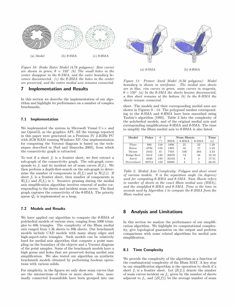
Figure 11: Primer Anvil Model (4.3k polygons): Modelboundary is shown in wireframe. The medial axis sheetsare in blue, rim curves in green, seam curves in magenta,θ = 150◦ (a) In the θ-SMA the sheets become disconnected,a thin sheet remains at the bottom (b) In the θ-HMA thesheets remain connected.

sheet. The models and their corresponding medial axes areshown in Figures 9 - 14. The polygonal meshes correspond-ing to the θ-SMA and θ-HMA have been smoothed usingTaubin’s algorithm [1995]. Table 2 lists the complexity ofthe polyhedral models, and of the original medial axis andcorresponding simplifications θ-HMA and θ-SMA. The timeto simplify the Blum medial axis to θ-HMA is also listed.

Model Polys θ Num Sheets Time

(◦) BMA θ-HMA θ-SMA (s)

Plate 990 150 1896 21 22 1.29

Rotor 4736 150 1365 41 17 1.23

Mount 2442 45 7455 536 283 2.43

Ridge-Rod 5012 120 30676 74 36 18.10

Anvil 4340 150 32102 4 4 17.51

Drivewheel 60712 150 89885 4 3 26.05

Table 2: Medial Axis Complexity: Polygon and sheet countof various models. θ is the separation angle (in degrees)used for computing θ-HMA and θ-SMA. Num Sheets refersto number of sheets in the exact Blum medial axis (BMA),and the simplified θ-HMA and θ-SMA. Time is the time inseconds used by Algorithm 1 to compute the θ-HMA from theBlum medial axis.

8 Analysis and Limitations

In this section we analyze the performance of our simplifi-cation algorithm. We highlight its computational complex-ity, give topological guarantees on the output and performcomparisons with some related algorithms for medial axissimplification.

8.1 Time Complexity

We provide the complexity of the algorithm as a function ofthe combinatorial complexity of the Blum MAT. A key stepin our simplification algorithm is the operation to check if asheet fi is a frontier sheet. Let |S(fi)| denote the numberof seam curves incident on fi, given by the number of sheetsadjacent to fi, and 〈|S(f)|〉 be the average number of seam

(a) Model (b) θ-HMA

Figure 12: CAD Mount (2.4k polygons), θ = 45◦: The sheetsemerging from the center of the vertical rod have low sepa-ration angle and have been removed. Note that the removaldoes not change the homotopy type.

curves of a sheet. Then the cost of checking if a sheet fi

is frontier is O(|S(fi)|). We first present the cost of Algo-rithm 3. In the worst case, the frontier sheet check is per-formed on each sheet fk adjacent to a sheet fi, i.e. |S(fi)|times. The cost of each frontier check is O(|S(fk)|). Thecost of adding or deleting a sheet from the priority queueQj is O(log |Qj |). Hence the cost of a single instance Al-

gorithm 3 is∑|S(fi)|

k=1 [O(|S(fk)|) + O(log |Qj |)]. Therefore,the cost of a single instance of Algorithm 2 is O(log |Qj |) +∑|S(fi)|

k=1 [O(|S(fk)|) + O(log |Qj |)] = O(〈|S(f)|〉2 +log |Qj |).A sheet fi can get added to the frontier set Qj at most|S(fi)| times. Hence, the number of iterations in Algo-

rithm 1 is at most∑|F|

i=1 |S(fi)| = O(|F|〈|S(f)|〉). More-over, the size of the frontier set is bounded by the numberof sheets, |Qj | ≤ |F|. Thus the total cost of the Algorithm 1is O(|F|〈|S(f)|〉3 + |F| log |F|〈|S(f)|〉). Typically, 〈|S(f)|〉isa constant, the size of the frontier set is much smaller than|F|, and the simplification cost is usually linear (or better)in |F|.

Figure 13: Cube with spherical void (1.5k polygons: A cut-out showing the cube and the spherical void in the center.The θ-HMA curves are drawn in magenta, θ = 180◦. Theθ-HMA remains connected, and preserves the void.

8.2 Comparisons with Other MAT Simplification Al-

gorithms

In this section, we compare some features of our MAT sim-plification algorithm with prior techniques. There are manyknown approaches for computing and simplifying the me-dial axis. It is hard to make direct comparisons between

all these algorithms, as different algorithms make varyingassumptions about the input and generate different kind ofapproximations.

The main feature of our approach is that we preserves thehomotopy type of the medial axis while allowing for signif-icant simplification of the medial axis. Our algorithm hasbeen applied to polyhedral models as input, and faithfullycaptures the medial axis near sharp edges and corners in theinput. Further, the algorithm preserves cavities correspond-ing to internal voids in the medial axis.

Some of the earlier analytic algorithms for MAT computa-tion are based on tracing the seam curves [Culver et al. 1999;Reddy and Turkiyyah 1995; Sherbrooke et al. 1996]. Thesealgorithms are relatively expensive and the worst case com-plexity is O(n3), where n is the number of features in theinput solid. In practice, they have been applied to polyhe-dral models with few thousand triangles and compute theBlum medial axis and not a simplification of the medialaxis. The adaptive subdivision algorithms [Vleugels andOvermars 1995; Etzion and Rappoport 2002] compute thegeneralized Voronoi Diagram, rather than a simplified me-dial axis. Further, these approaches may not be able tohandle polyhedral models with internal voids.

The surface sampling approaches, such as [Amenta et al.2001; Dey and Zhao 2002], take a point sampling on thesurface as input and approximate the medial axis using theVoronoi diagram. Robust and efficient methods for comput-ing the Voronoi diagram for point samples are well known. Itis hard to make a direct comparison, as the output generatedby these algorithms is different than our approaches whichcompute a distance field on a spatial grid. Many times thealgorithms based on a point samples of the boundary maynot be able to generate a good quality of approximation ofthe medial axis near the sharp features of the polyhedralmodel. The convergence of the Voronoi diagram to the me-dial axis with a finite discrete sampling has been proven,and extended algorithms have been proposed to generategood quality approximations for CAD models [Dey and Zhao2002]. However, these methods guarantee a convergence tothe medial axis in the limit, and may not provide topologi-cal guarantees on the computed medial axis approximation.Tam and Heidrich [2003] describe an iterative algorithm tosimplify the medial axis of polyhedral models while avoidingsome topological artifacts during the construction. Theirwork builds upon point sampling approaches, and has beenapplied to scanned models without many sharp features.There are no guarantees on the homotopy equivalence ofthe medial axis. Furthermore, the pruning algorithm needsto perform expensive global operations for topology preser-vation.

The λ-medial axis [Chazal and Lieutier 2004] provides a sim-plification of the medial axis for any open bounded shape inR

n with homotopy equivalence to the original medial axis.The constraints on λ depend on the critical points in thegradient field of the distance function. An ε-sampling of theboundary of the shape is required, the choice of ε dependson different heuristics. Also, a single value of λ may not beappropriate to provide significant simplification for the en-tire shape. We are not aware of a practical implementationof this method. Attali et al. [2004] acknowledge these openissues and suggest a nested sequence of λ-Voronoi graphswith different values of λ for portions of the shape. In fact,a λ-medial axis with a small value of λ can be used as theoriginal medial axis for our simplification algorithm, which

(a) Model (b) Blum Medial Axis (c) Medial Axis Closeup

(d) θ-HMA sheets, θ = 150◦ (e) θ-HMA sheets, θ = 90◦ (f) θ-HMA sheets closeup, θ = 90◦

Figure 14: DriveWheel model (60k Polygons) and medial axis at different resolutions: Artificial noise was added to the model.Rim curves are shown in green, seam curves are shown in magenta. (a) The Model, with the front faces shown in wireframe(b) Blum medial axis, black box highlights the zoomed in region (c) A closeup highlighting the tiny sheets corresponding to theunstable parts. (d) Sheets of the θ-HMA, θ = 150◦. Connectivity of the model and all holes are preserved. (e) Sheets of theθ-HMA, θ = 90◦, black box highlights the zoomed in region (f) A closeup of the θ-HMA, θ = 90◦, showing the stable subset ofthe medial axis.

subsequently allows significant simplification while preserv-ing homotopy equivalence.

8.3 Limitations

Our approach has a few limitations. Our simplification algo-rithm depends on a spatial subdivision scheme to computethe Voronoi graph of the polyhedron. Similar to [Etzion andRappoport 2002], the subdivision scheme generates a topo-logically accurate Voronoi diagram in absence of degenera-cies. In degenerate configurations, the algorithm computesan approximate Voronoi graph which may not preserve ho-motopy equivalence to the original polyhedral model. Themeasure of stability that depends on separation angles, pro-vides scale invariance but may retain noisy features if theyexhibit high separation angles. Our simplification algorithmuses a greedy approach for pruning the unstable parts of themedial axis and a global minimum of the stability measureis not guaranteed. The elementary primitive in our pruningalgorithm is a sheet, and the amount of simplification is in-fluenced by the size of sheets. Finally, the simplified medialaxis is not unique for a fixed value of θ, but depends on thepruning order. Actually, determining a unique order for it-erative pruning for 3D models using topological constraintsis still an open problem [Pizer et al. 2003].

9 Conclusions and Future Work

We have presented a medial axis approximation, the θ-HMA,that computes a stable subset of Blum’s medial axis, andpreserves the homotopy type of Blum’s medial axis. Thestability of the medial axis is guided by a separation anglecriterion, which has been well studied. For polyhedral mod-els, we present a formal characterization of the relationshipbetween the stability of medial axis junctions and seams tothe stability of incident sheets, based on separation angles.Our algorithm computes a bounded measure of stability of amedial axis sheet using discrete sampling. The constructionof the θ-HMA is based on an iterative pruning algorithmwhich uses efficient local tests.

There are several avenues of future work. We would liketo study other medial axis simplification criteria in conjunc-tion to separation angles. We would also like to computea θ-HMA with better guarantees on the global minimum ofthe stability measures, possibly leading to a unique prun-ing order. We would like to extend our algorithm to han-dle degenerate configurations of the Voronoi diagram, bothin terms of topology of the θ-HMA and the stability rela-tionship between incident parts of the medial axis. We areinterested in applying the simplification algorithm to othermedial axis approximations. Finally, we would like to ex-plore applications of the θ-HMA such as mesh generationand shape analysis.

Acknowledgments

This research is supported in part by ARO Contract DAAD19-02-1-0390, and W911NF-04-1-0088, NSF Awards0400134, 0118743, DARPA and RDECOM ContractN61339-04-C-0043, DOD Prostate Cancer Research Pro-gram DAMD17-03-1-0134 and Intel Corporation. We thankAjith Mascarenhas and the UNC GAMMA group for manyuseful discussions and support. We are also grateful to thereviewers for their feedback.

References

Amenta, N., Choi, S., and Kolluri, R. K. 2001. The power crust.

In Proc. ACM Symposium on Solid Modeling and Applications,

249–260.

Attali, D., Boissonat, J.-D., and Edelsbrunner, H. 2004. Stability

and computation of the medial axis. In Mathematical Founda-

tions of Scientific Visualization, Computer Graphics, and Mas-

sive Data Exploration. Springer-Verlag.

Blanding, R., Brooking, C., Ganter, M., and Storti, D. 1999. A

skeletal-based solid editor. In Proc. ACM Symposium on Solid

Modeling and Applications, 141–150.

Blum, H., and Nagel, R. 1978. Shape description using weighted

symmetric axis features. Pattern Recognition 10 , 167–180.

Blum, H. 1967. A transformation for extracting new descriptors of

shape. In Models for the Perception of Speech and Visual Form,

W. Wathen-Dunn, Ed. MIT Press, 362–380.

Chazal, F., and Lieutier, A. 2004. Stability and homotopy of a subset

of the medial axis. In Proc. ACM Symposium on Solid Modeling

and Applications.

Chazal, F., and Soufflet, R. 2004. Stability and finiteness properties

of medial axis and skeleton. Journal of Control and Dynamical

Systems 10, 2, 149–170.

Culver, T., Keyser, J., and Manocha, D. 1999. Accurate computation

of the medial axis of a polyhedron. In Proc. ACM Symposium on

Solid Modeling and Applications, 179–190.

Culver, T. 2000. Accurate Computation of the Medial Axis of a

Polyhedron. PhD thesis, Department of Computer Science, Uni-

versity of North Carolina at Chapel Hill.

Dey, T. K., and Zhao, W. 2002. Approximate medial axis as a Voronoi

subcomplex. In Proc. ACM Symposium on Solid Modeling and

Applications, 356–366.

Dimitrov, P., Damon, J. N., and Siddiqi, K. 2003. Flux invariants

for shape. In International Conference on Computer Vision and

Pattern Recognition.

Du, H., and Qin, H. 2004. Medial axis extraction and shape ma-

nipulation of solid objects using parabolic PDEs. In Proc. ACM

Symposium on Solid Modeling and Applications.

Etzion, M., and Rappoport, A. 2002. Computing Voronoi skeletons of

a 3-d polyhedron by space subdivision. Computational Geometry:

Theory and Applications 21, 3 (March), 87–120.

Foskey, M., Garber, M., Lin, M., and Manocha, D. 2001. A voronoi-

based hybrid planner. Proc. of IEEE/RSJ Int. Conf. on Intelli-

gent Robots and Systems.

Foskey, M., Lin, M., and Manocha, D. 2003. Efficient computation of

a simplified medial axis. Proc. of ACM Solid Modeling, 96–107.

Giblin, P., and Kimia, B. 2000. A formal classification of 3D medial

axis points and their local geometry. In Proc. IEEE Computer So-

ciety Conference on Computer Vision and Pattern Recognition,

566–573.

Kimmel, R., Shaked, D., Kiryati, N., and Bruckstein, A. M. 1995.

Skeletonization via distance maps and level sets. Computer Vision

and Image Understanding 62, 3, 382–391.

Kruse, B. 1991. An exact sequential Euclidean distance algorithm

with application to skeletonizing. In 7th Scandinavian Conference

on Image Analysis (SCIA ’91), 517–524.

Lam, L., Lee, S.-W., and Chen, C. Y. 1992. Thinning methodologies—

A comprehensive survey. IEEE Transactions on Pattern Analysis

and Machine Intelligence 14, 9, 869–885.

Leymarie, F. F., and Kimia, B. B. 2001. The shock scaffold for repre-

senting 3D shape. In Visual Form 2001, Springer-Verlag, 216–229.

Lecture Notes in Computer Science, no. LNCS 2059.

Lieutier, A. 2003. Any open bounded subset of Rn has the same

homotopy type than its medial axis. In Proc. ACM Symposium

on Solid Modeling and Applications, 65–75.

Malandain, G., and Fernandez-Vidal, S. 1998. Euclidean skeletons.

Image and Vision Computing 16 , 317–327.

Meyer, F. 1979. Cytologie quantitative et morphologie

Mathematique. PhD thesis, Ecole des Mines.

Milenkovic, V. 1993. Robust construction of the Voronoi diagram of a

polyhedron. In Proc. 5th Canad. Conf. Comput. Geom., 473–478.

Naf, M., Kubler, O., Kikinis, R., Shenton, M., and Szekely, G. 1996.

Characterization and recognition of 3D organ shape in medical im-

age analysis using skeletonization. In MMBIA96, MEDIAL AXES.

Ogniewicz, R. L., and Kubler, O. 1995. Hierarchic Voronoi skeletons.

Pattern Recognition 28, 3, 343–359.

Pizer, S. M., Siddiqi, K., Szekely, G., Damon, J. M., and Zucker,

S. W. 2003. Multiscale medial loci and their properties. Interna-

tional Journal of Computer Vision 55 , 155–179.

Reddy, J., and Turkiyyah, G. 1995. Computation of 3D skeletons

using a generalized Delaunay triangulation technique. Comput.

Aided Design 27, 9, 677–694.

Shaham, A., Shamir, A., and Cohen-Or, D. 2004. Medial axis based

solid representation. In Proc. ACM Symposium on Solid Modeling

and Applications.

Sheehy, D. J., Armstrong, C. G., and Robinson, D. J. 1995. Comput-

ing the medial surface of a solid from a domain Delaunay triangu-

lation. In Proc. Symposium on Solid Modeling and Applications.

Sheffer, A., Etzion, M., Rappoport, A., and Bercovier, M. 1998.

Hexahedral mesh generation using the embedded voronoi graph.

7th International Meshing Roundtable, 347–364.

Sherbrooke, E. C., Patrikalakis, N. M., and Brisson, E. 1996. An

algorithm for the medial axis transform of 3d polyhedral solids.

IEEE Trans. Visualizat. Comput. Graph. 2, 1 (Mar.), 45–61.

Siddiqi, K., B.B., K., and Shu, C.-W. 1997. Geometric shock-capturing

eno schemes for subpixel interpolation, computation and curve evo-

lution. Graphical Models and Image Processing 59, 5, 278–301.

Siddiqi, K., Bouix, S., Tannenbaum, A., and Zucker, S. W. 2002.

Hamilton-Jacobi skeletons. International Journal of Computer

Vision 48 , 215–231.

Spanier, E. H. 1989. Algebraic Topology. Springer.

Sud, A., and Manocha, D. 2005. A simple algorithm for bounded-

error approximation of voronoi diagrams of 3D polygonal models.

Tech. rep., University of North Carolina-Chapel Hill.

Suresh, K. 2003. Automating the CAD/CAE dimensional reduction

process. In Proc. ACM Symposium on Solid Modeling and Ap-

plications, 76–85.

Tam, R., and Heidrich, W. 2003. Shape simplification based on the

medial axis transform. IEEE Visualization.

Taubin, G. 1995. A signal processing approach to fair surface design.

In Proc. of ACM SIGGRAPH, 351–358.

Vleugels, J., and Overmars, M. 1995. Approximating generalized

Voronoi diagrams in any dimension. Tech. Rep. UU-CS-1995-14,

Department of Computer Science, Utrecht University.

Yang, Y., Brock, O., and Moll, R. N. 2004. Efficient and robust

computation of an approximated medial axis. In Proc. ACM Sym-

posium on Solid Modeling and Applications, 15–24.

Zhang, Y. Y., and Wang, P. S. P. 1993. Analytical comparison of

thinning algorithms. Int. J. Pattern Recognit. Artif. Intell. 7 ,

1227–1246.