horizontal well drilling history in ca - california ... · pdf filehorizontal well drilling...
TRANSCRIPT

343
Appendices
Appendix H
Horizontal Well Drilling History in CA
In California, horizontal wells are used with and without well stimulation. This appendix discusses the historic application of horizontal wells without well stimulation, followed by an assessment of recent horizontal well installation activity. Historic and recent stimulation of horizontal wells is discussed in Section 3.2 regarding hydraulic fracturing. The following is a review of the use of horizontal wells in California.
Historical Horizontal Well Utilization
The first horizontal-well-drilling technology was developed in the 1920s, but the development of the technology led to limited use until the mid-1980s, followed by a rapid increase through the 1990s, when they became common (Ellis et al., 2000). Many thousands of horizontal wells had been installed in the United States by the mid-1990s (Joshi and Ding, 1996).
Modern methods of horizontal well drilling, as described in Section 2.2.2, have a number of applications in oil production (Ellis et al., 2000); in the shale oil and gas basins elsewhere in the country, their use is principally to allow production from relatively thin, impermeable shales. However, in California, the applications are more varied. They can have greater contact area with the petroleum-containing reservoir in near-horizontal layered geologic systems. Horizontal wells can also more readily intersect more natural fractures in the reservoir that may conduct oil, owing not only to their intersecting more of the reservoir than a vertical well, but also because fractures are typically perpendicular to rock strata, and so are nearly vertical in near-horizontal strata.
Horizontal wells can parallel water-oil or oil-gas contacts, and so can be positioned along their length to produce more oil, without drawing in water or gas, than is possible from a vertical well. Due to their orientation parallel to geologic strata, horizontal wells can improve sweep efficiency during secondary or tertiary oil recovery, which involves the injection of other fluids, such as steam, to mobilize oil to a production well. A horizontal well also provides for more uniform injection to a particular stratum. On the production side, a horizontal well provides a more thorough interception of the oil mobilized by the injection. Vertical wells are more readily bypassed by mobilized oil due to variation in the permeability of the reservoir rock. Similar to being better positioned to intercept oil mobilized by injection, horizontal wells are also better positioned to intercept oil draining by gravity through a reservoir.

344
Appendices
An example of a thin reservoir development in California is the installation of a horizontal well in a Stevens Sand layer of the Yowlumne field in the southern San Joaquin Basin, which was a layer too thin to be developed economically using vertical wells. It was completed in 1991 at a true depth of over 3,400 m (11,200 ft) with a 687 m (2,252 ft) lateral. The well tripled the production rate from the previous vertical wells in the reservoir (Marino and Shultz, 1992).
The use of horizontal wells to improve the efficiency of steam injection for oil recovery began in the early 1990s. Steam injection reduces the viscosity of oil, allowing it to flow more readily to production wells. For example, in 1990 and 1991, three horizontal wells were installed by Shell Western Exploration and Production in 45° dipping (tilted) units with a long history of steam injection in the Midway Sunset field in the San Joaquin Basin. Two of the wells were installed with 121 m (400 ft) sloping laterals. These wells produced two to three times more oil as nearby vertical wells, but cost two to three times more, and so did not provide an economic benefit. The third well, with a longer horizontal lateral of 213 m (700 ft), produced six times more oil than nearby vertical wells and so was more economically successful (Carpenter and Dazet, 1992).
Shell Western Exploration and Production also installed horizontal wells in a shallow, tilted (dipping) geologic bed in the Coalinga field in the San Joaquin Basin in the early 1990s. Steam injection with oil production via vertical wells started in this zone in the late 1980s. The horizontal wells were installed in the same reservoir but deeper along the tilted bed. The wells were initially operated with steam cycling. This process entails injecting steam for a period, then closing the well to let the steam continue to heat the oil and reservoir, then opening the well and producing oil. However, the increase in production resulting from steam cycling was lower than expected. Vertical wells for continuous steam injection were subsequently installed shallower along the tilted bed from the horizontal wells. This resulted in a large sustained production rate that justified the horizontal wells, which led to considering further opportunities for installing horizontal wells in the Coalinga field (Huff, 1995).
By the late 1990s, horizontal well installation projects for production of shallow oil, using vertical steam injectors, involved tens of wells each. Nearly 100 horizontal wells were installed in shallow sands containing heavy (viscous) oil in the Cymric and McKittrick fields in the San Joaquin Basin from the late 1990s to early 2000s. These wells were installed in association with vertical wells that injected steam to reduce the viscosity of the oil by heating, allowing it to flow to the horizontal wells. The wells were installed in phases, allowing optimization with each phase that reduced the cost per well by 45% by the last phase (Cline and Basham, 2002). By the late 2000s and early 2010s, drilling programs in reservoirs with steam injection included as many as hundreds of wells. For instance, over 400 horizontal wells were installed in the Kern River field in the San Joaquin Basin between 2007 and 2013, targeting zones identified with low oil recovery to date. These wells provided a quarter of the field’s daily production (McNaboe and Shotts, 2013).
345
Appendices
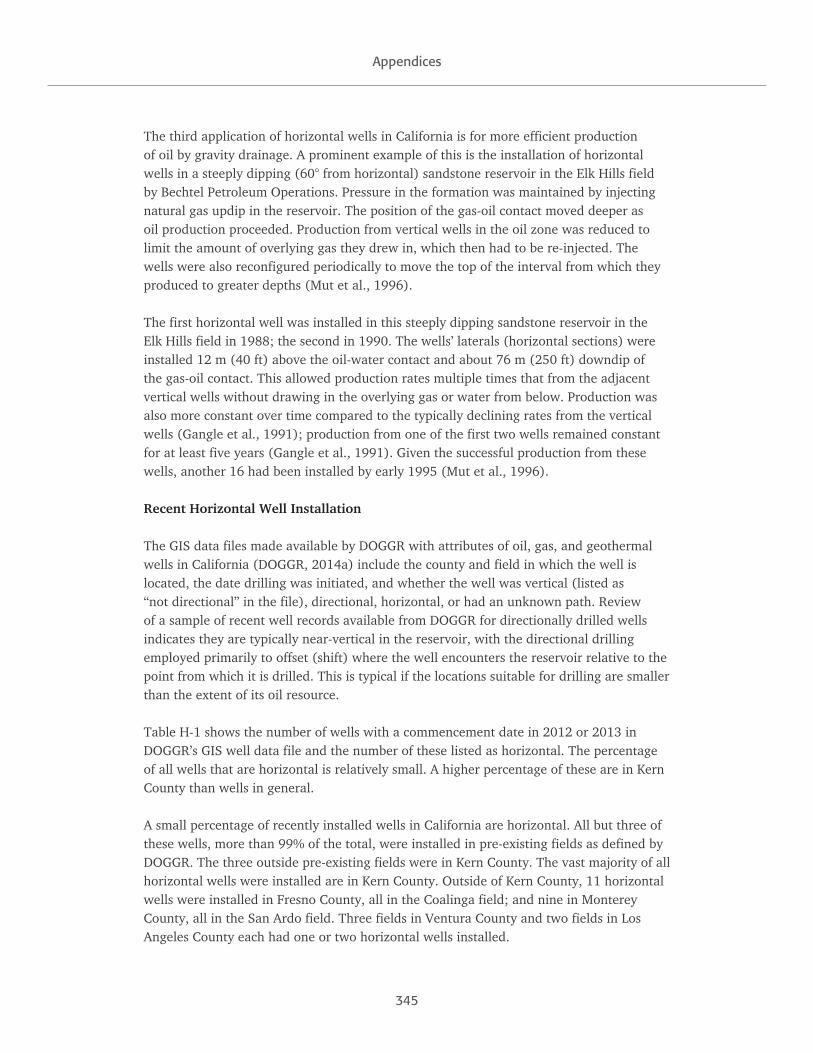
The third application of horizontal wells in California is for more efficient production of oil by gravity drainage. A prominent example of this is the installation of horizontal wells in a steeply dipping (60° from horizontal) sandstone reservoir in the Elk Hills field by Bechtel Petroleum Operations. Pressure in the formation was maintained by injecting natural gas updip in the reservoir. The position of the gas-oil contact moved deeper as oil production proceeded. Production from vertical wells in the oil zone was reduced to limit the amount of overlying gas they drew in, which then had to be re-injected. The wells were also reconfigured periodically to move the top of the interval from which they produced to greater depths (Mut et al., 1996).
The first horizontal well was installed in this steeply dipping sandstone reservoir in the Elk Hills field in 1988; the second in 1990. The wells’ laterals (horizontal sections) were installed 12 m (40 ft) above the oil-water contact and about 76 m (250 ft) downdip of the gas-oil contact. This allowed production rates multiple times that from the adjacent vertical wells without drawing in the overlying gas or water from below. Production was also more constant over time compared to the typically declining rates from the vertical wells (Gangle et al., 1991); production from one of the first two wells remained constant for at least five years (Gangle et al., 1991). Given the successful production from these wells, another 16 had been installed by early 1995 (Mut et al., 1996).
Recent Horizontal Well Installation
The GIS data files made available by DOGGR with attributes of oil, gas, and geothermal wells in California (DOGGR, 2014a) include the county and field in which the well is located, the date drilling was initiated, and whether the well was vertical (listed as “not directional” in the file), directional, horizontal, or had an unknown path. Review of a sample of recent well records available from DOGGR for directionally drilled wells indicates they are typically near-vertical in the reservoir, with the directional drilling employed primarily to offset (shift) where the well encounters the reservoir relative to the point from which it is drilled. This is typical if the locations suitable for drilling are smaller than the extent of its oil resource.
Table H-1 shows the number of wells with a commencement date in 2012 or 2013 in DOGGR’s GIS well data file and the number of these listed as horizontal. The percentage of all wells that are horizontal is relatively small. A higher percentage of these are in Kern County than wells in general.
A small percentage of recently installed wells in California are horizontal. All but three of these wells, more than 99% of the total, were installed in pre-existing fields as defined by DOGGR. The three outside pre-existing fields were in Kern County. The vast majority of all horizontal wells were installed are in Kern County. Outside of Kern County, 11 horizontal wells were installed in Fresno County, all in the Coalinga field; and nine in Monterey County, all in the San Ardo field. Three fields in Ventura County and two fields in Los Angeles County each had one or two horizontal wells installed.

346
Appendices
Table H-1. Number of all wells and horizontal wells whose installation was listed as
commencing in 2012 and 2013 (DOGGR, 2014b).
All wells Horizontal wells
#
With path type
#% of wells
with path type% in Kern
County% in pre-
existing fieldsIn California In Kern County
# % # %
5,143 4,384 85 4,297 84 308 7 92 99
References
Carpenter, D.E., and S.C. Dazet (1992), Horizontal Wells in a Steamdrive in the Midway Sunset Field, in Proceedings of SPE/DOE Enhanced Oil Recovery Symposium, Society of Petroleum Engineers.
Cline, V., and M. Basham (2002), Improving Project Performance in a Heavy Oil Horizontal Well Project in the San Joaquin Valley, California, in Proceedings of SPE International Thermal Operations and Heavy Oil Symposium and International Horizontal Well Technology Conference, Society of Petroleum Engineers.
DOGGR (Division of Oil, Gas and Geothermal Resources) (2014a), Well Stimulation Treatment Disclosure Index. ftp://ftp.conservation.ca.gov/pub/oil/Well_Stimulation_Treatment_Disclosures/20140507_CAWellStimulationPublicDisclosureReport.xls
Ellis, P.D., G.M. Kniffin, and J.D. Harkrider (2000). Application of Hydraulic Fractures in Openhole Horizontal Wells. In: Proceedings of SPE/CIM International Conference on Horizontal Well Technology, Society of Petroleum Engineers.
Gangle, F.J., K.L. Schultz, and G.S. McJannet (1991), Horizontal Wells in a Thick Steeply Dipping Reservoir at NPR-1, Elk Hills, Kern County, California. In: Proceedings of SPE Western Regional Meeting, Society of Petroleum Engineers.
Huff, B. (1995), Coalinga Horizontal Well Applications: Present and Future. In: Proceedings of SPE International Heavy Oil Symposium, Society of Petroleum Engineers.
Joshi, S.D., and W. Ding (1996), Horizontal Well Application: Reservoir Management. In: Proceedings of International Conference on Horizontal Well Technology, Society of Petroleum Engineers.
Marino, A.W., and S.M. Shultz (1992), Case Study of Stevens Sand Horizontal Well. In: Proceedings of SPE Annual Technical Conference and Exhibition, Society of Petroleum Engineers.
McNaboe, G.J., and N.J. Shotts (2013), Horizontal Well Technology Applications for Improved Reservoir Depletion, Kern River Oil Field. In: AAPG Annual Convention and Exhibition, Pittsburgh, Pennsylvania, May 19-22, 2013, AAPG.
Mut, D.L., D.M. Moore, T.W. Thompson, and E.M. Querin (1996), Horizontal Well Development of a Gravity Drainage Reservoir, 26R Pool, Elk Hills Field, California. In: Proceedings of SPE Western Regional Meeting, Society of Petroleum Engineers.
347
Appendices
Appendix I
Procedure for Searching Well Records for Indications
of Hydraulic Fracturing
Well records are publicly available from the California Department of Oil, Gas, and Geothermal Resources (DOGGR) in the form of scans without searchable text (DOGGR, undated a). Through application of optical character recognition software, DOGGR provided versions of scanned records with searchable text for wells with first production or injection after 2001 (Bill Winkler, DOGGR, personnel communication).
Due to the large number of wells in Kern County, a sample of records was chosen for application of character recognition and subsequent searching. To define the sample proportion, the proportion of all records indicating hydraulic fracturing was presumed to be 20%. Given this presumption, the sample proportion for Kern County was selected to provide 95% confidence that the estimated proportion was within 2% of the actual proportion, using a finite population correction factor.
For some other counties, such as Fresno, digital records were available for all the wells. For the remaining counties, digital records were not available for all wells. Like for Kern County, this resulted in searching a sample of records for these counties. For some of them, such as Los Angeles and Orange counties, the proportion of wells with previously available digitized records was too small to provide a sufficiently constrained estimate of the proportion of wells hydraulically fractured. DOGGR scanned and provided additional records for these counties.
Searching the well record set provided by DOGGR resulted in data regarding the number of wells hydraulically fractured over time. Records potentially indicating that a well was hydraulically fractured were identified using the search term “frac.” The space after the term avoided occurrences of the term “fracture,” which appears in the template information on some forms, and consequently the term is not correlated with wells that have been hydraulically fractured.
Records containing “frac” were reviewed to determine if hydraulic fracturing indeed occurred. The term “frac” was found to correctly identify more records of hydraulic fracturing than other potential terms, such as “fracture,” “stimulation,” “stage,” and “frack.” The few records containing the latter term also all included the term “frac.”

348
Appendices
For Kern County, 90% of all the well records containing the term “frac” were confirmed as indicating hydraulic fracturing had occurred. In the other 10% of records, the term was used for other purposes, such as to describe geologic materials or to refer to the fracture gradient (the minimum fluid pressure per depth that will fracture the rock in a particular location). For the rest of the state, 63% of the records containing “frac” were confirmed as indicating hydraulic fracturing had taken place, and the term was used for other purposes in the other 37% of records. These percentages are based on weighting the result for each county by the estimated number of records containing “frac” in that county. For individual counties with at least five records containing “frac,” the percentage confirmed as indicating hydraulic fracturing ranged from 13% (Santa Barbara County) to 73% (Solano County).
In some records, the term “frac” was found to also indicate a Frac-Pack was completed. As described previously, placement of a Frac-Pack occurs above the fracturing pressure, and results in a fracture (the “frac”) propagated from the well filled with introduced granular material (the “pack”). The purpose of a Frac-Pack is to bypass formation damage resulting from drilling and/or control production of granular material from the formation.
“HRGP,” standing for “high rate gravel pack,” was identified in records for a number of wells in Los Angeles County. This is an alternate term for a Frac-Pack. The Los Angeles County records were searched for this term with the result that 16 in addition to those containing the term “frac” were identified. Review confirmed each of these records indicated a fracturing operation had occurred. All the records regarded wells in the Inglewood field. Subsequently, all of the well records were searched for “HRGP.” Only one additional record not also containing the term “frac” was identified. This regarded a well in Kern County.
For records indicating hydraulic fracturing occurred, the operation was assigned to the date of the well’s first production, or first injection if first production was not available. For hydraulically fractured wells with first production and injection, the fracturing date in almost all the records is closer to the first production date.
Reference
DOGGR (Division of Oil, Gas and Geothermal Resources) (undateda). OWRS – Search Oil and Gas Well Records. Available at http://owr.conservation.ca.gov/WellSearch/WellSearch.aspx

349
Appendices
Appendix J
Number of Well Records Searched for Indication of
Hydraulic Fracturing
The following tables list the number of well first produced or injected from 2002 through September 2013, the number and % of these wells whose records were searched for reports of hydraulic fracturing (HF), and the number and percent of records that contained reports of hydraulic fracturing. The first table lists basins and the second counties with at least one well with first production or injection during this time period.
Table K-1 lists the estimated number of well records indicating hydraulic fracturing by sedimentary basin. Table K-2 lists the estimated number of well records indicating hydraulic fracturing by county.
Table J-1. Annual average total number of well records, and total number and percent of well
records identified as indicating hydraulic fracturing by basin and for the state for wells with
first production or injection from 2002 to 2013.
Basin
2002-2006 2007-2011 2012-2013
New wells
Searched HF recorded New wells
Searched HF recorded New wells
Searched HF recorded
# % # % # % # % # % # %
Cuyama 21 2 10% 0 0% 11 1 9% 0 0% 1 0 0% - -
Eel River 9 9 100% 0 0% 2 2 100% 0 0% 0 - - - -
Hollister-Sargent
0 - - - - 8 4 50% 0 0% 0 - - - -
Los Angeles 661 528 80% 153 29% 639 503 79% 75 15% 428 331 77% 32 10%
onshore 457 341 75% 106 31% 431 317 74% 34 11% 246 176 72% 14 8%
offshore 204 187 92% 47 25% 208 186 89% 41 22% 182 155 85% 18 12%
Sacramento 458 455 99% 15 3% 545 534 98% 59 11% 28 22 79% 0 0%
Salinas 156 18 12% 3 17% 405 121 30% 0 0% 118 7 6% 0 0%
San Joaquin 13,355 2,318 17% 591 25% 13,372 2,377 18% 523 22% 5,681 1,266 22% 372 29%
Santa Barbara-Ventura
130 126 97% 12 10% 347 339 98% 65 19% 154 149 97% 28 19%
Santa Maria 126 126 100% 12 10% 344 337 98% 65 19% 147 142 97% 28 20%
Santa Barbara-Ventura
4 0 0% - - 3 2 67% 0 0% 7 7 100% 0 0%
California 14,865 3,490 23% 775 22% 15,520 4,012 26% 724 18% 6,543 1,814 28% 432 24%

350
Appendices
Table J-2. Annual average total number of well records, and total number and percent of well
records identified as indicating hydraulic fracturing by county and for the state for wells with
first production or injection from 2002 to 2013.
County
2002-2006 2007-2011 2012-2013
New wells
Searched HF recorded New wells
Searched HF recorded New wells
Searched HF recorded
# % # % # % # % # % # %
Alameda 1 1 100% 0 0% 0 0 - 0 - 0 0 - 0 -
Butte 6 6 100% 0 0% 9 7 78% 0 0% 0 0 - 0 -
Colusa 61 61 100% 1 2% 114 109 96% 10 9% 16 10 63% 0 0%
Contra Costa 5 5 100% 1 20% 8 8 100% 0 0% 0 0 - 0 -
Fresno 463 463 100% 2 0% 664 664 100% 4 1% 166 166 100% 3 2%
Glenn 63 63 100% 2 3% 125 124 99% 11 9% 4 4 100% 0 0%
Humboldt 9 9 100% 0 0% 2 2 100% 0 0% 0 0 - 0 -
Kern 12,821 1,785 14% 589 33% 12,655 1,663 13% 516 31% 5,506 1,093 20% 369 34%
Kings 11 11 100% 0 0% 10 10 100% 2 20% 3 2 67% 0 0%
Los Angeles 697 588 84% 157 27% 659 549 83% 64 12% 434 341 79% 26 8%
Madera 7 7 100% 0 0% 16 16 100% 0 0% 1 1 100% 0 0%
Merced 1 1 100% 0 0% 1 1 100% 0 0% 0 0 - 0 -
Monterey 156 18 12% 3 17% 405 121 30% 0 0% 118 7 6% 0 0%
Orange 50 26 52% 2 8% 56 30 54% 13 43% 18 14 78% 6 43%
Sacramento 73 72 99% 6 8% 46 45 98% 4 9% 5 5 100% 0 0%
San Benito 1 1 100% 0 0% 1 1 100% 0 0% 0 0 - 0 -
San Joaquin 43 43 100% 0 0% 13 11 85% 1 9% 3 3 100% 0 0%
San Luis Obispo
45 17 38% 0 0% 17 6 35% 0 0% 20 0 0% - -
Santa Barbara 55 18 33% 1 6% 185 125 68% 2 2% 113 38 34% 0 0%
Santa Clara 0 0 - 0 - 7 3 43% 0 0% 0 0 - 0 -
Solano 72 71 99% 4 6% 53 53 100% 10 19% 1 1 100% 0 0%
Stanislaus 2 2 100% 0 0% 0 0 - 0 - 0 0 - 0 -
Sutter 66 66 100% 1 2% 161 161 100% 24 15% 0 0 - 0 -
Tehama 77 77 100% 0 0% 19 19 100% 0 0% 2 2 100% 0 0%
Tulare 7 7 100% 0 0% 13 12 92% 0 0% 2 1 50% 0 0%
Ventura 40 40 100% 6 15% 271 264 97% 63 24% 130 125 96% 28 22%
Yolo 32 31 97% 0 0% 10 8 80% 0 0% 1 1 100% 0 0%
Yuba 1 1 100% 0 0% 0 0 - 0 - 0 0 - 0 -
California 14,865 3,490 23% 775 22% 15,520 4,012 26% 724 18% 6,543 1,814 28% 432 24%

351
Appendices
Appendix K
Estimated Number of Well Records Indicating Hydraulic
Fracturing By Geographic Area
Table K-1 lists the estimated number of well records indicating hydraulic fracturing by sedimentary basin. Table K-2 lists the estimated number of well records indicating hydraulic fracturing by county.
For geographic areas with more than zero wells fractured during a time period, the 95% confidence bounds were calculated using a logit transform. For geographic areas with zero wells fractured during a time period, the 95% confidence bounds were calculated using the rule of three. The positive confidence increment was taken as the theoretical maximum if it were less than either the logit or rule of three results. The theoretical maximum is calculated by assuming all the wells with unavailable records were fractured.

352
Appendices
Table K-1. Annual average number of wells with first production or injection from 2002 to
2013 by basin. Estimated annual average rate of wells fractured, percent of all wells fractured,
and 95% confidence interval (CI) for the fracturing rate based on searching well records. No
fracturing rate is shown if less than one eighth of the well records were available for searching.
“NA” for the percentage fractured indicates no wells had first injection or production in the time
period. No CI is shown if no rate was estimated or all the well records were searched. Analysis of
more recent data from various sources indicates actual hydraulic fracturing rates may be up to
twice as high.
Basin
2002-2006
2007-2011
2012-2013
New wells
Frac.wells
% frac 95% CINew wells
Frac.wells
% frac 95% CINew wells
Frac.wells
% frac 95% CI
Cuyama 4.2 - - - 2.2 - - - 0.6 - - -
Eel River 1.8 0.0 0% - 0.4 0.0 0% - 0.0 0.0 NA -
Hollister-Sargent
0.0 0.0 NA - 1.6 0.0 0% 0.0-0.2 0.0 0.0 NA -
Sonoma- Livermore
0.2 0.0 0% - 0.0 0.0 NA - 0.0 0.0 NA -
Los Angeles 132 38.3 29% 36.0-40.6 128 19 15% 17.3-21.0 245 23.6 10% 20.2-27.6
onshore 91.4 28.4 31% 26.2-30.7 86.2 9.2 11% 7.8-10.9 140.6 11.2 8% 8.5-14.6
offshore 40.8 10.3 25% 9.5-11.0 41.6 9.2 22% 8.4-10.0 104.0 12.1 12% 10.3-14.3
Sacramento 91.6 3.0 3% - 109 11.9 11% 11.9-11.9 16.0 0.0 0% 0.0-0.1
Salinas 31.2 - - - 81.0 0.0 0% 0.0-0.0 67.4 - - -
San Joaquin 2,671 847 32% 795-899 2,674 787 29% 735-841 3,246 1,064 33% 986-1,146
Santa Maria 15 0.5 3% 0.2-2.0 36.8 0.6 2% 0.4-1.2 74.3 0.0 0% 0.0-0.0
Santa Barbara-Ventura
26.0 2.5 10% 2.4-2.7 69.4 13.3 19% 13.0-13.8 88.0 16.5 19% 16.0-17.6
California 2,973 895 30% 837-961 3,104 832 27% 778-891 3,739 1,104 30% 1,022-1,192

353
Appendices
Table K-2. Annual average number of wells with first production or injection from 2002 to 2013
by county. Estimated annual average rate, percent, and 95% confidence interval (CI) for the
rate of wells fractured based on searching well records. No fracturing rate is shown if less than
one eighth of the well records were available for searching. NA” for the percentage fractured
indicates no wells had first injection or production in the time period. No CI is shown if no rate
was estimated or all the well records were searched. Analysis of more recent data from various
sources indicates actual rates may be up to twice as high.
County
2002-2006 2007-2011 2012-2013
New wells
Frac. wells
% frac.
95% CINew wells
Frac. wells
% frac.
95% CINew wells
Frac. wells
% frac.
95% CI
Alameda 0.2 0.0 0% - 0.0 0.0 NA - 0.0 0.0 NA -
Butte 1.2 0.0 0% - 1.8 0.0 0% 0.0-0.1 0.0 0.0 NA -
Colusa 12 0.2 2% - 22.8 2.1 9% 2.0-2.4 9.1 0.0 0% 0.0-0.2
Contra Costa 1.0 0.2 20% - 1.6 0.0 0% - 0.0 0.0 NA -
Fresno 92.6 0.4 0% - 133 0.8 1% - 94.9 1.7 2% 1.7-1.7
Kern 2,564 846 33% 795-899 2,531 785 31% 734-839 3,146 1,062 34% 985-1,143
Kings 2.2 0.0 0% - 2.0 0.4 20% 0.4-0.4 1.7 0.0 0% 0.0-0.6
Los Angeles 139 37.2 27% 35.3-39.2 132 15.4 12% 14.0-16.9 248 18.9 8% 15.9-22.4
Madera 1.4 0.0 0% - 3.2 0.0 0% - 0.6 0.0 0% -
Merced 0.2 0.0 0% - 0.2 0.0 0% - 0.0 0.0 NA -
Monterey 31.2 - - - 81.0 0.0 0% - 67.4 - - -
Orange 10 0.8 8% 0.4-1.9 11.2 4.9 43% 3.5-6.3 10 4.4 43% 3.4-5.7
Sacramento 15 1.2 8% 1.2-1.3 9 0.8 9% 0.8-0.9 2.9 0.0 0% -
San Benito 0.2 0.0 0% - 0.2 0.0 0% - 0.0 0.0 NA -
San Joaquin 8.6 0.0 0% - 2.6 0.2 9% 0.2-0.5 1.7 0.0 0% -
San Luis Obispo
9.0 0.0 0% - 3.4 0.0 0% 0.0-0.1 11.4 - - -
Santa Barbara 11 0.6 6% 0.2-2.8 37.0 0.6 2% 0.4-1.3 64.6 0.0 0% -
Santa Clara 0.0 0.0 NA - 1.4 0.0 0% 0.0-0.2 0.0 0.0 NA -
Solano 14 0.8 6% 0.8-0.9 11 2.0 19% 2.0-2.0 0.6 0.0 0% -
Stanislaus 0.4 0.0 0% - 0.0 0.0 NA - 0.0 0.0 NA -
Sutter 13 0.2 2% - 32.2 4.8 15% 4.8-4.8 0.0 0.0 NA -
Tehama 15 0.0 0% - 3.8 0.0 0% - 1.1 0.0 0% -
Tulare 1.4 0.0 0% - 2.6 0.0 0% 0.0-0.1 1.1 0.0 0% 0.0-0.6
Ventura 8.0 1.2 15% - 54.2 12.9 24% 12.6-13.4 74.3 16.6 22% 16.0-17.7
Yolo 6.4 0.0 0% - 2.0 0.0 0% 0.0-0.1 0.6 0.0 0% -
Yuba 0.2 0.0 0% - 0.0 0.0 NA - 0.0 0.0 NA -
California 2,973 895 30% 837-961 3,104 832 27% 778-891 3,739 1,104 30% 1,022-1,192


355
Appendices
Appendix L
Well-Record Result Data Set
The data listing the API number for the wells considered in the well record search are provided in both Excel and tab-delimited text format. These wells have a first production date between 2002 and near the end of 2013, or a first injection date if no first production date, which is also listed, along with the basin, county, field, and area where that well is located, and the pool it was open to on that date. Whether the record for a well was searched, if the record indicated hydraulic fracturing occurred, and if the hydraulic fracturing consisted of a frac-pack is also listed.
The first production and injection date source file provided by the California Department of Oil, Gas, and Geothermal Resources has more than one record for some wells. The start dates are specific to the combination of a well and pool, so if a well is recompleted in a new pool it will have an additional start date. The data in this appendix include only the first occurrence of a well’s production and injection dates, and the pool for that date. The full data can be found at http://ccst.us/publications/WST.


357
Appendices
Appendix M
Integrated hydraulic fracturing data set regarding occurrence,
location, date, and depth
Data regarding the occurrence, location, date and depth of hydraulic fracturing was integrated from the following data sources:
1. Well stimulation disclosures to the California Division of Oil, Gas, and Geothermal Resources (DOGGR),
2. South Coast Air Quality Management District (SCAQMD) well work data,
3. FracFocus,
4. FracFocus data compiled by SkyTruth,
5. Well record search results combined with first production or injection date (described above),
6. Central Valley Regional Water Quality Control Board (CVRWQCB) well work data, and
7. DOGGR geographic information system (GIS) well layer.
Each of these sources is described in the section 3.5 of the associated report. The data are provided in both Excel and tab-delimited text formats. The tables include all the data from all the sources. The first columns contain the most accurate version of each datum from among all the sources in the authors’ judgment and a code indicating the source of that datum. The data source codes are as follows:
AW = DOGGR’s AllWells GIS layer CR = Hydraulic fracturing disclosures (completion reports) provided to DOGGR CV = CVRWQCB data set FF = FracFocus FI = First injection FP = First production SC = SCAQMD data set WR = Well record search

358
Appendices
Some of the data sources contain more than one record for a well, such as DOGGR’s AllWells GIS layer. This appendix lists the data from the first record for each well with regard to occurrence and location, and the minimum value for date and depth. The full data can be found at http://ccst.us/publications/WST.

359
Appendices
Appendix N
Pools with Production Predominantly Facilitated By Hydraulic Fracturing
This appendix contains two lists of pools for which more than half the wells starting production from 2002 through late 2013 are estimated to be hydraulically fractured. The first list (“non-GS”) regards oil and gas production pools. The second list (“GS”) regards gas storage pools. The lists provide the following for each pool:
• The number of wells entering production during the time period
• The number of these wells for which records were received
• The fraction of wells with records received
• The number of records indicating hydraulic fracturing
• The fraction of records indicating hydraulic fracturing
• The fraction of such records adjusted for underreporting,
• Oil, gas, and water production from 2002 through May 2014
• The oil, gas, and water production multiplied by the fraction of records indicating hydraulic fracturing adjusted for underreporting
• Average oil and gas production per well per day
• The gas-oil ratio
The underreporting adjustment was made by taking the minimum of one or 1.63 times the fraction of records indicating hydraulic fracturing. The underreporting adjustment factor is equal to 150, which is the estimated average number of well fractured per month statewide, divided by 92, which is the estimated average number of records indicating fracturing statewide (shown on Figure 3-10 and discussed in related text).
The oil, gas, and water production were summed from sum by pool data available through the California Department of Oil, Gas, and Geothermal Resources online production and injection portal (http://opi.consrv.ca.gov/opi/opi.dll). The full data can be found at http://ccst.us/publications/WST.


361
Appendices
Appendix O
Water Volume Per Stimulation Event
The available data regarding the volume of water used per stimulation were aggregated from FracFocus, CVRWQCB well work, SCAQMD well work, and the well stimulation disclosures. For some wells, multiple values were available. If the volume was different and the dates sufficiently different, these were judged to be refracturing operations and were included. If the volume or date was the same, these were judged to be two records regarding the same operation. Judgment was used in selecting which data to include. The full data can be found at http://ccst.us/publications/WST.

363
Appendices
Appendix P
California Oil Fields and Source Rocks
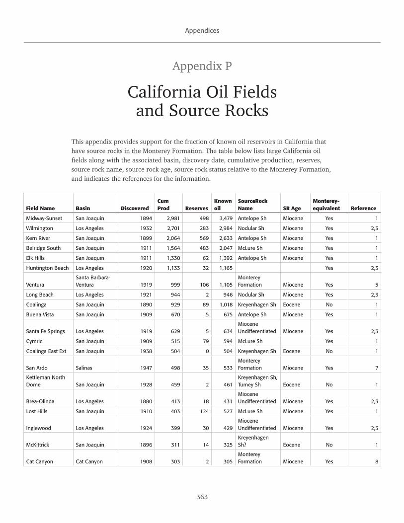
This appendix provides support for the fraction of known oil reservoirs in California that have source rocks in the Monterey Formation. The table below lists large California oil fields along with the associated basin, discovery date, cumulative production, reserves, source rock name, source rock age, source rock status relative to the Monterey Formation, and indicates the references for the information.
Field Name Basin DiscoveredCum Prod Reserves
Known oil
SourceRock Name SR Age
Monterey-equivalent Reference
Midway-Sunset San Joaquin 1894 2,981 498 3,479 Antelope Sh Miocene Yes 1
Wilmington Los Angeles 1932 2,701 283 2,984 Nodular Sh Miocene Yes 2,3
Kern River San Joaquin 1899 2,064 569 2,633 Antelope Sh Miocene Yes 1
Belridge South San Joaquin 1911 1,564 483 2,047 McLure Sh Miocene Yes 1
Elk Hills San Joaquin 1911 1,330 62 1,392 Antelope Sh Miocene Yes 1
Huntington Beach Los Angeles 1920 1,133 32 1,165 Yes 2,3
VenturaSanta Barbara-Ventura 1919 999 106 1,105
Monterey Formation Miocene Yes 5
Long Beach Los Angeles 1921 944 2 946 Nodular Sh Miocene Yes 2,3
Coalinga San Joaquin 1890 929 89 1,018 Kreyenhagen Sh Eocene No 1
Buena Vista San Joaquin 1909 670 5 675 Antelope Sh Miocene Yes 1
Santa Fe Springs Los Angeles 1919 629 5 634Miocene Undifferentiated Miocene Yes 2,3
Cymric San Joaquin 1909 515 79 594 McLure Sh Yes 1
Coalinga East Ext San Joaquin 1938 504 0 504 Kreyenhagen Sh Eocene No 1
San Ardo Salinas 1947 498 35 533Monterey Formation Miocene Yes 7
Kettleman North Dome San Joaquin 1928 459 2 461
Kreyenhagen Sh, Tumey Sh Eocene No 1
Brea-Olinda Los Angeles 1880 413 18 431Miocene Undifferentiated Miocene Yes 2,3
Lost Hills San Joaquin 1910 403 124 527 McLure Sh Miocene Yes 1
Inglewood Los Angeles 1924 399 30 429Miocene Undifferentiated Miocene Yes 2,3
McKittrick San Joaquin 1896 311 14 325Kreyenhagen Sh? Eocene No 1
Cat Canyon Cat Canyon 1908 303 2 305Monterey Formation Miocene Yes 8

364
Appendices
Field Name Basin DiscoveredCum Prod Reserves
Known oil
SourceRock Name SR Age
Monterey-equivalent Reference
Mount Poso San Joaquin 1926 300 6 306 Antelope Sh Miocene Yes 1
Hondo OffshoreSanta Barbara-Ventura 1969 286 31 317
Monterey Formation Miocene Yes 8
Dominguez Los Angeles 1923 274 52 326 Nodular Shale Miocene Yes 2,3
Dos CuadrasSanta Barbara-Ventura 1968 263 2 265
Monterey Formation Miocene Yes 8
Coyote West Los Angeles 1909 253 0 253 Yes 2,3
Torrance Los Angeles 1922 226 5 231 Nodular Sh Miocene Yes 2,3
Cuyama South Cuyama 1949 255 4 259 Vacqueros Oligocene No 4
Seal Beach Los Angeles 1924 215 6 221 Nodular Sh Miocene Yes 2,3
Kern Front San Joaquin 1912 215 18 233 Antelope Sh Miocene Yes 1
Santa Maria Valley Santa Maria 1934 207 1 208Monterey Formation Miocene Yes
Montebello Los Angeles 1917 205 6 211Undifferentiated Miocene shales Miocene Yes 2,3
Richfield Los Angeles 1919 203 3 206Undifferentiated Miocene shales Miocene Yes 2,3
Orcutt Santa Maria 1901 181 12 193Monterey Formation Miocene Yes 8
Point Arguello Offshore Santa Maria 1981 179 29 208
Monterey Formation Miocene Yes 6
Coles Levee North San Joaquin 1938 165 1 166 Antelope Sh Miocene Yes 1
RinconSanta Barbara-Ventura 1927 163 3 166
Monterey Formation Miocene Yes 5
South MountainSanta Barbara-Ventura 1916 159 6 165
Monterey Formation Miocene Yes
Edison San Joaquin 1928 150 6 156 Antelope Sh Miocene Yes 1
Beverly Hills Los Angeles 1900 150 9 159 Yes 2,3
Belridge North San Joaquin 1912 147 17 164Kreyenhagen Sh? Eocene No 1
Pescado OffshoreSanta Barbara-Ventura 1970 132 15 147
Monterey Formation Miocene Yes 8
Fruitvale San Joaquin 1928 126 9 135 Antelope Sh Miocene Yes 1
Rio Bravo San Joaquin 1937 118 1 119 Antelope Sh Miocene Yes 1
San MiguelitoSanta Barbara-Ventura 1931 118 7 125
Monterey Formation Miocene Yes 5
Coyote East Los Angeles 1909 116 4 120 Yes 2,3
Greeley San Joaquin 1936 116 1 117 Antelope Sh Miocene Yes 1
Round Mountain San Joaquin 1947 115 7 122 Antelope Sh Miocene Yes 1
Yowlumne San Joaquin 1974 111 2 113 Antelope Sh Miocene Yes 1
Carpinteria Off-shore
Santa Barbara-Ventura 1966 107 2 109
Monterey Formation Miocene Yes 8
365
Appendices
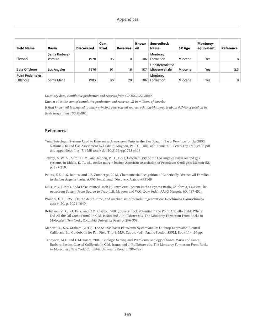
Field Name Basin DiscoveredCum Prod Reserves
Known oil
SourceRock Name SR Age
Monterey-equivalent Reference
ElwoodSanta Barbara-Ventura 1928 106 0 106
Monterey Formation Miocene Yes 8
Beta Offshore Los Angeles 1976 91 16 107Undifferentiated Miocene shale Miocene Yes 2,3
Point Pedernales Offshore Santa Maria 1983 86 20 106
Monterey Formation Miocene Yes 8
Discovery date, cumulative production and reserves from CDOGGR AR 2009
Known oil is the sum of cumulative production and reserves, all in millions of barrels.
If field known oil is assigned to likely principal reservoir oil source rock non-Monterey is about 9.74% of total oil in
fields larger than 100 MMBO
References
Total Petroleum Systems Used to Determine Assessment Units in the San Joaquin Basin Province for the 2003 National Oil and Gas Assessment by Leslie B. Magoon, Paul G. Lillis, and Kenneth E. Peters (pp1713_ch08.pdf and appendices files; 7.1 MB total) doi:10.3133/pp1713.ch08
Jeffrey, A. W. A., Alimi, H. M., and Jenden, P. D., 1991, Geochemistry of the Los Angeles Basin oil and gas systems, in Biddle, K. T., ed., Active margin basins: American Association of Petroleum Geologists Memoir 52, p. 197-219.
Peters, K.E., L.S. Ramos, and J.E. Zumberge, 2013, Chemometric Recognition of Genetically Distinct Oil Families in the Los Angeles basin: AAPG Search and Discovery Article #41149
Lillis, P.G. (1994). Soda Lake-Painted Rock (!) Petroleum System in the Cuyama Basin, California, USA In: The petroleum System-From Source to Trap, L.B. Magoon and W.G. Dow (eds), AAPG Memoir, 60, 437-451.
Philippi, G.T., 1965, On the depth, time, and mechanism of petroleumgeneration: Geochimica Cosmochimica acta v. 29, p. 1021-1049.
Robinson, V.D., B.J. Katz, and C.M. Clayton, 2001, Source Rock Potential in the Point Arguello Field: Where Did All the Oil Come From? In C.M. Isaacs and J. Rullkötter eds. The Monterey Formation From Rocks to Molecules: New York, Columbia University Press p. 296-309.
Menotti, T., S.A. Graham (2012). The Salinas Basin Petroleum System and Its Outcrop Expression, Central California. In: Guidebook for Fall Field Trip 1, M.V. Caputo (ed), Pacific Section SEPM, Book 114, 29 pp.
Tennyson, M.E. and C.M. Isaacs, 2001, Geologic Setting and Petroleum Geology of Santa Maria and Santa Barbara Basins, Coastal California In C.M. Isaacs and J. Rullkötter eds. The Monterey Formation From Rocks to Molecules: New York, Columbia University Press p. 206-229.


367
Appendices
Appendix Q
Unit Conversion Table1 Barrel = 0.158987 Cubic Meters (m3)
1 Cubic Foot (ft3) = 0.02831685 Cubic Meters (m3)
1 Cubic Mile (mi3) = 4.16818 Cubic Kilometers (km3)
1 Foot (ft) = 0.3048 Meters (m)
1 Inch (in) = 2.54 Centimeters (cm)
1 Gallon (gal) = 0.00378541 Cubic Meters (m3)
1 Acre-foot = 1,233.4 Cubic Meters (m3)
1 Miles (mi) = 1.609344 Kilometers (km)
1 Square Mile (mi2) = 2.589988 Square Kilometers (km2)
1 Nautical Mile = 1.852 Kilometers (km)
1 Millidarcy (md) = 9.87 x 10⁻¹⁶ Square meters (m2)
1 Pound per Square Inch (psi) = 6.89476 x 10⁻⁶ Gigapascals (GPa)