hospital financial pressures and the health … · the sponsors of the sp-sp center are the ......

IESE Business School-University of Navarra - 1

HOSPITAL FINANCIAL PRESSURES AND THE HEALTH OF THE UNINSURED.

WHO GETS HURT? THE CASE OF CALIFORNIA

Núria Mas

IESE Business School – University of Navarra Av. Pearson, 21 – 08034 Barcelona, Spain. Phone: (+34) 93 253 42 00 Fax: (+34) 93 253 43 43 Camino del Cerro del Águila, 3 (Ctra. de Castilla, km 5,180) – 28023 Madrid, Spain. Phone: (+34) 91 357 08 09 Fax: (+34) 91 357 29 13 Copyright © 2009 IESE Business School.

Working PaperWP-789 March, 2009

IESE Business School-University of Navarra

The Public-Private Center is a Research Center based at IESE Business School. Its mission is to develop research that analyses the relationships between the private and public sectors primarily in the following areas: regulation and competition, innovation, regional economy and industrial politics and health economics.

Research results are disseminated through publications, conferences and colloquia. These activities are aimed to foster cooperation between the private sector and public administrations, as well as the exchange of ideas and initiatives.

The sponsors of the SP-SP Center are the following:

• Accenture • Ajuntament de Barcelona • Caixa Manresa • Cambra Oficial de Comerç, Indústria i Navegació de Barcelona • Consell de l’Audiovisual de Catalunya • Departamento de Economía y Finanzas de la Generalitat de Catalunya • Departamento de Innovación, Universidades y Empresa de la Generalitat de Catalunya • Diputació de Barcelona • Endesa • Fundació AGBAR • Garrigues • Mediapro • Microsoft • Sanofi Aventis • VidaCaixa

The contents of this publication reflect the conclusions and findings of the individual authors, and not the opinions of the Center's sponsors.




Núria Mas1

Abstract

The United States relies on charitable medical care to serve the uninsured, most of which is offered by hospitals that act as providers of last resort and that constitute the “safety net”. This paper analyzes the effect that hospital financial stress has on the health of the uninsured. In particular we look at managed care. Managed care penetration has often been blamed for increasing financial pressures on hospitals, and previous work has shown that safety net hospitals have been affected more severely by it. Our findings are threefold: first, we find that managed care financial pressures encourage charity care patients to concentrate in public hospitals. Second, we find that these hospitals, in turn, see a decrease in their quality of care in areas where managed care penetration is stronger. Finally we also find that managed care diffusion has a negative effect on the quality of care received by the uninsured – as measured by the probability of dying after a heart attack – and of those that go to government hospitals.

Keywords: uninsured, hospitals, financial care, quality.

1 Professor of Economics, IESE

NOTE: I thank David M. Cutler; Bruno Cassiman, and the many participants in the Harvard public finance research seminar and workshop and in the ASHE meetings for comments on a previous draft. Financial support from Ministerio de Educación y Ciencia SEJ2006-11833.




I. Introduction In 2007, there were nearly 46 million uninsured individuals in the United States – that is about 18% of the population under 65.1 Traditionally, the United States has relied on an institutional “safety net” – comprised largely of government, teaching hospitals and hospitals located in poor areas – to provide at least the basic health care needs to this distressed population. For many years, hospitals were able to finance the provision of charity care through a complex system of cross-subsidies where privately insured patients were charged higher prices that helped cover indigent care costs2 (Aaron, 1991; Cutler, 1995). Hence, hospital financial health plays a crucial role in its ability to provide charity care.

The goal of this paper is to shed some light on the effect that hospital financial stress might have on the quality of care received by the uninsured.

For this, we will focus on the financial pressures imposed by managed care. Duke (1996) already identified managed care as a “primary force” affecting hospital revenues. By imposing strict cost-control mechanisms to doctors and hospitals, managed care has threatened the delicate net of cross-subsidies to finance charity care, challenging the future financial viability and survival of historical providers of health care to the uninsured.

We look at the case of managed care because managed care penetration has been one of the most important changes in the United States health care market in the last decades and has played a crucial role in shaping today’s healthcare marketplace. It has changed all the physician’s practice patterns (Baker and Shankarkumar, 1997) and the competition in the health care market. For instance, by initially paying prices about 30% below those paid by traditional insurers (Cutler and Barro, 1997), managed care organizations contributed to restricting doctors’ wages, not only within the managed care network but also in the whole health care market, and raising competition amongst providers. Understanding the effect of

1 DeNavas-Walt, C.B. Proctor, and J. Smith, “Income, Poverty, and Health Insurance Coverage in the United States: 2007”, United States Census Bureau; August 2008. 2 A study of the American Hospital Association calculates that the average paying hospital patient subsidizes charity care by paying a “hidden tax” of 10.6%.

2 - IESE Business School-University of Navarra

managed care on the health of the uninsured is a first step in helping us comprehend the role that current financial pressures could have on the health of this distressed population.

Some previous work has already related the financial pressures imposed by managed care on the provision of charity care by hospitals. For instance, authors such Thorpe and Phelps (1988) or Frank et al. (1990) have shown that an increase in competition reduces the provision of charity care. Currie and Fahr (2004) demonstrate that higher managed care penetration rates lead to an increase in the share of uninsured patients treated by public hospitals at the expense of losing the more profitable Medicaid patients to private ones. Richardson (2000) finds a negative impact of managed care on access to care for the poor. Mas (2009) showed that managed care disproportionately encouraged the closure of safety net hospitals as well as those hospital services most commonly used by the uninsured, such as emergency rooms, obstetrics and alcohol and drug treatments, having an important negative effect on their access to care.

However, very little is known about the effect that hospital financial incentives have on the quality of care received by the uninsured. The goal of this paper is to go one step further and analyze whether managed care, by imposing financial pressures on hospitals, has had a negative effect on the health of the uninsured in the United States. For this analysis, we use data on all hospital discharges in California for 1985 and 1995. We chose this period because it encompasses the most relevant years for the introduction of managed care in California.3

One of the major obstacles when looking at quality of care involves its measurement. Here, we focus on the proportion of patients with acute myocardial infarction (AMI) who die in the hospital. We use this measure for several reasons. First, because death is a generally accepted quality measure and it is a relatively common outcome for heart attacks. Second, AMI cases are not immediately fatal if the patient is rapidly admitted to a hospital and, hence, the hospital intervention is crucial. Finally, this measure of hospital quality has already been used in the literature (McClellan and Staiger, 2000).

Our results are twofold: first, at the hospital level, we find that managed care contributes to a shift of charity care patients toward government hospitals, confirming the findings of Currie and Fahr (2004) regarding charity care. Moreover, the results also seem to point toward the possibility of a trade-off between the number of charity care patients and the quality of care provided. Government hospitals, now receiving a higher proportion of non-paying patients while keeping their budget almost constant, experience a decline in the quality of care they provide.

Second, at the patient level, our results show that managed care penetration has a negative impact on the healthcare outcomes (measured as the probability of dying after an AMI) of uninsured patients and of those that attend government hospitals.

The rest of the paper is laid out as follows: Section 2 presents the conceptual framework and the hypothesis. The data used is described in section 3. Section 4 includes the methodology and the results and, finally, section 5 concludes.

3 This is the period most commonly looked at in the managed care literature (see, for instance, Mas and Seinfeld (2008); Currie and Fahr (2004), Baker and Shankarkumar (1997), etc.). Moreover, since then the managed care penetration has stabilized and the health care market place has been affected by its changes.


II. Conceptual Framework and Hypotheses

a) Managed care

One of the most important changes in hospital payment incentives in the United States has been the shift from traditional insurance to managed care. The growth of managed care insurance has been dramatic, with the percentage of privately insured Americans with a managed care contract rising from 27% in 1988 to 93% in 2001.4 Between 1986 and 1995 the proportion of privately insured who were enrolled in a Health Maintenance Organization (henceforth, HMO) contract went from 15 to 43%.

Managed care imposed a strong emphasis on cost containment and it gave rise to competitive pressures among providers to reduce costs (Baker, 1999; Baker and Shankarkumar, 1997).

There are two main differences between traditional insurance plans and managed care. First, traditional insurers barely monitored utilization as they allowed providers to decide the treatment and paid them on a fee-for-service basis. Managed care plans generally establish a capped payment or a fixed salary for physicians and use contractual means to enforce price discipline and utilization control on hospitals and specialists. This arrangement changes providers’ incentives as they no longer make money on the volume of patients treated and services provided, but by decreasing the use and costs of their services. For instance, managed care organizations paid prices about 30% below those paid by traditional insurers (Cutler and Barro, 1997). There are several methods used to control utilization: managed care plans use primary care physicians as “gatekeepers”, requiring their previous referral before the enrollees can consult a specialist. Many plans also limit the number of hospital days and require physicians to follow some established guidelines to treat a certain diagnosis.

Second, traditional insurance plans allowed patients unlimited access to the providers of their choice. Managed care removes equal choice of doctors and hospitals by establishing a network of approved providers. This restriction may be direct – covering its members only when they see the selected providers – or indirect – using a co-payment system to encourage the insured to use the services provided by their own network. As the number of managed care enrollees goes up, so does the importance of access to the network, since the hospitals that do not belong to it will not get managed care patients. In turn, the importance of the network increases the bargaining power of managed care organizations.

Current plans include several types of organizations. In the HMOs, patients are only allowed to visit those providers that belong to the network in exchange for a prepaid premium and, generally, with very low or no copayments. Here providers are usually paid on a capped basis. Preferred Providers Organizations (PPOs) correspond to another type of managed care organization where patients are allowed to use a limited number of providers with no copayment but, if they want to use a physician outside the network, the insurance company will pay a limited amount to that provider. Physicians are reimbursed on a discounted fee-for-service basis. The Independent Practice Association (IPA) arrangement contracts with physicians on a non-exclusive basis, so that they are allowed to cover patients who also have other types of insurance contracts. Finally, the Point-of-service (POS) corresponds to an arrangement where 4 Trends & Indicators in the Changing Health Care Marketplace, 2002 – Chartbook.


the patient can choose providers but she would pay a higher copayment if the chosen provider does not belong to the network.

b) The Uninsured and the Safety Net

The number of uninsured in the United States has been rising since 1987. In 1987 there were 31.8 million uninsured. In 1998, 44 million Americans lacked any regular health insurance coverage and in 2007 this number rose up to almost 46 million (18% of the non-elderly).5 The proportion of uninsured varies greatly with income. In 2007, about two-thirds of the uninsured were poor or near poor (Kaiser, 2008). In 1998, 34.7% of the population below 200% of the poverty line were uninsured, while only 4.6% of those with income above 400% of the poverty line lacked health insurance (Current Population Survey).

The uninsured are less likely to have a regular source of care, are more likely to report that they have not received the needed care and wait until they are seriously ill to seek medical care (American College of Physicians-American Society of Internal Medicine, 2000). In 2000, 20% of the United States uninsured reported not getting medical care for serious conditions.6

Because the United States lacks universal health coverage, it relies on charitable medical care to serve the uninsured. Most of this charity care is provided by hospitals that serve as providers of last resort. These providers that organize and deliver a significant level of care to the uninsured and Medicaid patients constitute the safety net. For many of the uninsured, access to care is possible thanks to the safety net, constituted mostly by public hospitals, teaching hospitals and those located in poor areas (Mas, 2009).

c) The Impact of Managed Care on the Health of the Uninsured

Managed care has affected the environment in which safety net providers operate. By imposing strict cost-control mechanisms, it has reduced hospital revenues (Duke, 1996) and it has threatened their ability to keep cross-subsidizing charity care through private insured patients. The reduction of the price paid by the privately insured makes it more difficult for the safety net hospitals to keep serving charity care patients.

Managed care may affect the health care received by the uninsured through several channels:

First, by encouraging the closure of safety net hospitals and of those services most commonly used by the uninsured, managed care can negatively affect access to care for charity care patients. Mas (2009) already found that managed care had a positive effect on the closure of safety net hospitals, both in the United States and in California. She also found that, for those hospitals that remained open, managed care had a positive effect on the closure of those services most commonly used by the uninsured (emergency rooms, obstetrics and alcohol and drug treatment centers). Interestingly, Mas also found that if a public hospital was the only public hospital in the metropolitan area (henceforth, “MSA”) it was more likely to keep operating.

A reduction on the number of safety net hospitals and their higher termination of these services traditionally used by the uninsured implies that the average patient in the area has to travel

5 United States Census Bureau. 6 Trends and Indicators in the Changing Healthcare Marketplace; Kaiser family foundation.


greater distances in order to obtain medical care. Currie and Reagan (1998) found that distance to hospital has significant effects on the utilization of preventive care among central-city black children, for which an additional mile to the hospital was associated with a 3% decline in their probability of having a checkup. Goodman et al. (1997) found that medical hospitalizations for patients living more than 30 minutes away from the hospital was 0.85 times the hospitalization of those living in a zip code with a hospital. Following this literature, a reduction of the number of hospitals and services traditionally used by the uninsured – and the consequent increase in the distance that patients have to travel to get medical care – could translate to a worsening of their health status.

Hence, the first mechanism through which managed care could affect the health of the uninsured is by worsening their access to health care. However, in order to determine the extent to which access to care has actually been affected, we need to check that uninsured patients do not shift to other hospitals to obtain charity care in those areas where managed care is stronger. For instance, they might shift to public hospitals, especially given the fact that they have been found to face important pressures to remain open if they are the only public hospital in the MSA. This corresponds to the first part of the empirical analysis.

The second mechanism relates to the quality of care received. Even if the uninsured shift now to the hospitals that remain open, those hospitals are subject to a financial squeeze, since now they have to supply more charity care with the same amount of revenues than before (or even less, due to the financial pressures). This might lead to a potential trade-off between quality and quantity of care. This will be the second part of the empirical analysis.

Finally, the ultimate goal of this paper is to analyze the effect that managed care has had on the health of the uninsured. Since managed care has been shown to affect different types of hospitals differently – mainly, safety net hospitals are affected more severely (Mas, 2009) – the important element here is to distinguish the effect of managed care on the health of those patients who lack health insurance (mainly through postponing their hospital visits due to managed care effect on the closure of safety net hospitals – the first mechanism) from the effect of managed care on the health of other patients who have insurance but just happen to go to a hospital that is now facing the trade-off mentioned in the second mechanism above. This is done in the third part of our analysis.

III. Data To further examine these questions we will focus on California. The first reason to do so is that, to measure quality of care, we need to use hospital discharge data. California was the only state that had such information available for us to use during this time period. We will use the California Hospital Discharge Data from the Office of Statewide Healthcare Planning and Development (OSHPD). It contains information on every hospital discharge (approximately 3.6 million per year), including the patient’s expected payer (self-pay, charity, Medicare, etc.), the patient’s diagnosis and whether the patient died in the hospital. The second reason is that California is a natural state to study because of its size and data availability and it also has a lot of variation regarding managed care penetration in its territory, which facilitates the identification of its effect. Moreover, Mas (2009) already found that, in California, the effect of managed care on hospital closures and the closure of those services most commonly used by the uninsured followed trends similar to the ones obtained using the whole United States data.


However, California differs from the rest of the United States in the fact that its managed care penetration has been stronger and is now a more mature phenomenon.

Charity care: We use the information on the patient’s expected payer from the OSHPD. We include as uncompensated care those patients whose expected source of payment is one of the following: self-pay, no charge or medically indigent. Some people consider as charity care those who receive Medicaid (Medi-Cal, in California) as well. For robustness checks, we will also look at the separated from the uncompensated care ones and then we will consider them together as well. In 1985, California teaching hospitals provided 38% of the MSA total charity care and served 35% of the total MSA Medi-Cal patients. Government-non-teaching hospitals provided 46% of the MSA charity care and 40% of Medi-Cal care, and non-public hospitals located in poor areas provided 7% and 15% of the MSA charity care and Medi-Cal care, respectively.

Managed care enrollment: To account for the effect of managed care on the quality of care for the uninsured, we use the share of the MSA population enrolled in HMOs, which has been the standard measure for managed care enrollment used in the literature – see, for instance Cutler and McClellan (1996); Baker (1997); Cutler and Sheiner (1998). We use data from the Baker estimates in managed care enrollment. Baker constructed estimates of county-level enrollment using data from the Group Health Association of America and he distributed HMO enrollment among the counties of its service area taking into account their population and the distance to the HMO headquarters. Moreover, in order to further lessen any potential problem, our analysis is done at the MSA level.

There is the possibility that some unobserved variables affect both the health of the uninsured and managed care enrollment. For instance, managed care organizations might be less willing to operate in areas where the uninsured population goes to the hospital more frequently. To correct for these potential endogeneity problems, we will also present our results instrumenting managed care enrollment by average firm size in the MSA. This is the usual instrument used in the literature (Baker, 1997; Baker and Brown, 1999; Mas and Seinfeld, 2008). It reflects the fact that larger firms are more likely to contract with managed care organizations to offer health care benefits to their employees than the smaller ones.

Quality of care: One of the major obstacles when looking at the quality of care involves its measurement. As a quality measure, we will use the proportion of patients with acute myocardial infarction (AMI, or heart attack) that die in the hospital. We focus on this particular diagnostic for several reasons. First, because death is a generally accepted quality measure and it is a relatively common outcome for heart attacks. Second, AMI cases are not immediately fatal if the patient is rapidly admitted to a hospital and, hence, the hospital intervention is crucial. Finally, this measure of hospital quality has already been used in the literature (McClellan and Staiger, 2000).

When looking at whether there is a trade-off between quality and quantity of charity care provided by hospitals, we will look at the change in the proportion of AMI patients who died in the hospital. Due to the technology improvements between 1985 and 1995, for the average hospital in California in 1995 the amount of patients dying of AMI was lower than the proportion that died in 1985. We will consider that a hospital experiences a worsening of the quality of its care if the improvement on AMI survival is lower than in the baseline case. Data comes from the OSHPD.


Hospital characteristics: One of the main elements to take into account is whether a hospital belongs to the safety net. Mas (2009) found that government hospitals, teaching hospitals and hospitals located in poor areas had a higher burden of charity care and were also the ones that provided care to a higher proportion of Medicaid7 patients. We will use a dummy for each one of those hospital types.

To determine if a hospital belongs to a poor neighborhood, we establish a ranking of the average income per capita in all the zip codes in California to determine the level corresponding to the thirty-third percentile. Then we compute the average per capita income for the five-mile radius area surrounding the hospital. If it lies below the thirty-third percentile level for the corresponding state, the hospital is considered to be located in a poor neighborhood.

Hospital data on public ownership and teaching status come form the American Hospital Association (AHA). We also include a dummy variable indicating whether the hospital is for profit or not-for-profit and we control for hospital size measured by the number of beds.

Finally, previous work has also found that managed care has a different effect for those hospitals that are the only ones of their type in the MSA, especially if they are the only public hospital in the metropolitan area. We will, then, define a dummy variably ONLY that is equal to one if the hospital if the only one of its type in the MSA.

Demographic characteristics: They include the logarithm of the average family income in the MSA, the percentage of population older than 65, the percentage of uninsured in the MSA and the percentage of the MSA population with Medicaid and Medicare. The demographic information comes from the Current Population Survey (CPS).

IV. Methods and Results

Testing whether Patients Shift to Public Hospitals where Managed Care is Stronger

Previous work has already shown that managed care leads to hospital closure, especially of safety net hospitals. It has also found that managed care encourages the closure of those services most commonly used by the uninsured. All these facts could lead to a worsening of their access to health care. However, for this to be the case we should be sure that charity care patients do not shift to other types of hospitals in areas where managed care is stronger. In order to determine whether charity care patients are shifting to public hospitals when managed care enrollment increases, we will look at the effect that managed care enrollment has on the share of the overall MSA charity care patients who go to each hospital. In particular, our dependent variable is the change of the percentage of the overall MSA charity care patients who go each hospital between 1985 and 1995 (Yi). We also look at alternative measure of charity care, since some argue that Medi-Cal8 patients should also be considered.

According to our hypothesis, the change in the proportion of charity care patients that a hospital has might depend on several relevant variables: on the evolution of managed care

7 Program funded by the federal government and the states whose goal is to provide health care to low income citizens. 8 Medicaid program in California.


penetration (HMO); on whether the hospital is in the safety net – government hospital (G), teaching hospital (T) or hospital located in a poor area (P), on hospital variables (SIZEi) or on the demographic characteristics of the area (DEM). Moreover, managed care might have a different effect for different types of hospitals. Actually, it has already been established that it has a stronger effect for the closures of hospitals and certain services for the safety net. Hence we will also include the interactions of managed care enrollment and hospital type. Finally, we also control for the possibility that a hospital that is the only (ONLY) one of its type in the whole metropolitan area might behave differently. For instance, if it is a public hospital, it might face strong pressure to remain open even if it is under financial stress. Hence, we will also interact the ONLY dummy by each hospital type.

Our empirical strategy uses the following specification:

liiiiiiimsaliii

iimsaiimsaiimsaimsai

GONLYTONLYPONLYONLYDEMSIZEGTP

GHMOTHMOPHMOHMOeCharityCarProportion

εψνϕληγρωθδβαφ

++++++++++∆+∆+∆+∆=∆

***

***)( ,,,,

liiiiiiimsaliii



GHMOTHMOPHMOHMOeCharityCarProportion


++++++++++∆+∆+∆+∆=∆

***

***)( ,,,,

In this specification, the baseline hospital is a non-traditional safety net one (non-government, non-teaching, and not located in poor areas).

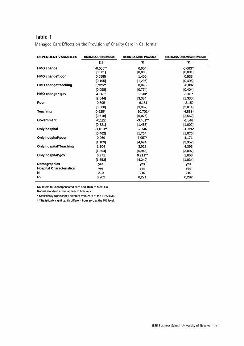
Results of the OLS regressions are presented in Table 1. The corresponding instrumental variable output is presented in Table A1 of the Appendix. The results are consistent. The first conclusion from Table 1 is that that managed care enrollment has a significantly negative effect on the share of the overall MSA charity care provided by the non-safety net hospitals.

The second conclusion is that our results confirm the Currie and Fahr (2001) findings and show that, as managed care penetration increases, a larger proportion of the MSA charity care is provided by government hospitals. In column [1], we can see that HMO penetration has a clear positive effect on the charity care market share for government hospitals. For instance, a one standard deviation increase in HMO enrollment would lead to a 63% higher rise in the share of MSA uninsured care provided by government hospitals between 1985 and 1995 than in the baseline non safety net hospitals.

The second columns of Table 1 looks at the effect of the growth managed care enrollment on the proportion of the MSA Medi-Cal patients served in each hospital. The conclusions are similar: Medi-Cal patients tend to concentrate more in government hospitals in areas where managed care penetration is stronger. Moreover, here, the effect of being the only government hospital in the metropolitan area is positive and significant. Finally, Column [3] of Table 1 considers as charity care both the Medi-Cal and uninsured patients. In this case a one standard deviation increase in HMO enrollment leads to a 38% higher rise in the share of charity care provided by government hospitals than in the baseline ones.

Table 1 confirms that public hospitals in metropolitan areas where managed care penetration is larger serve a bigger proportion of the MSA uninsured.

Managed Care Effect on the Quality of Care Provided by Safety Net Hospitals

The concentration of uninsured in public hospitals in areas with higher HMO could have important financial consequences for these hospitals, since now they serve a higher number of non-paying patients using (in the best case scenario) the same revenues. Our second hypothesis suggests the possibility of a trade-off between quantity of charity care and quality of care provided. Here we will look at whether the quality of care provided by government hospitals – which are now providing


more charity care than before – has worsened with respect to the baseline case in areas where managed care enrollment has increased more.

As we explained in section III, our measure of hospital quality of care is the proportion of patients who die after a heart attack. Ceteris paribus, all other things being equal, a higher proportion would indicate that the quality is worse. One should take into account that, due to technological change, the number of patients who die after a heart attack has decreased over time. Hence, when we say that the quality of a hospital has worsened, what we mean is that the proportion of patients who die after an AMI has improved less than in the baseline case.

To analyze the effect that the increase in managed care has had on the quality of public hospitals, our dependent variable will be the change in the proportion of patients who die after a heart attack (AMI).

Discharge data tell us whether the patient left the hospital dead or alive. However, one always has to consider the possibility of some hospitals discharging their patients early, which could led them to simply dying at home instead of at the hospital. In order to address this concern, we will look also at those patients who left the hospital after five days or fewer. Finally, one should also take into account that not all hospitals are equally prepared to treat a heart attack and that it might simply be the case that, where there is more managed care, more hospitals have closed their intensive care cardiac units (this is not what Mas, 2009, finds, but we should still make sure that this possibility does not distort the results). If this were the case, one could argue that what happens is that, where there is more managed care, there is a higher probability that the patient gets taken to the “wrong” hospital type (without cardiac intensive care) after a heart attack. In order to take this into account, we will also present our results including only those hospitals that have a cardiac intensive care unit.

Our empirical strategy uses the following specification:

liiiiiiimsaliii



GHMOTHMOPHMOHMOadAfterAMIoportionDe


++++++++++∆+∆+∆+∆=∆

***

***)(Pr ,,,,

liiiiiiimsaliii



GHMOTHMOPHMOHMOadAfterAMIoportionDe


++++++++++∆+∆+∆+∆=∆

***

***)(Pr ,,,,

Table 2 presents the results. Note that, since the dependent variable is the change in the percentage of patients who die, a positive coefficient indicates a worsening of the hospital quality.

The first and second columns include all the urban non-federal general hospitals in California. The third and fourth ones include only the hospitals that have intensive cardiac care units as reported in the AHA Annual Survey. Columns 1 and 3 report the OLS coefficients and columns 2 and 4 include the IV instrumental variables results. They are consistent.

The first two columns of Table 2 show that, in areas where managed care enrollment has increased more, government hospitals have experienced a lower improvement in their quality than the rest of hospitals. Compared to the baseline, a standard deviation increase of the HMO enrollment between 1985 and 1995 would imply that the improvement in quality as between these years is 27% lower in government hospitals.

These results remain when we consider only the proportion of patients who die after an AMI and that have been admitted to hospitals that have specialized cardiac units. The OLS and the IV results are reported in columns [3] and [4]. Interestingly in this case, the results also show that the rise in the relative proportion of patients who die after a heart attack in government


hospitals compared to the baseline is of particular severity if it is the only public hospital in the MSA. In Table 1, we saw that these hospitals were receiving even more charity care patients.

Finally, these results are consistent with those obtained when we considered only those patients who have stayed in the hospital fewer than six days after suffering an AMI. They are reported in columns 1b, 2b, 3b and 4b. Columns 1b and 2b include all the hospitals and columns 3b and 4b contain only those hospitals with cardiac intensive care units. The coefficients for the interaction of change in HMO enrollment and the government hospital dummy are still positive and significant indicating that government hospitals have worsened their quality between 1985 and 1995 in areas where managed care is growing more.

These results seem to indicate that there is a trade-off between the number of charity care patients and the quality of care provided. The effect of an increase in managed care penetration is stronger for public hospitals, which are precisely the ones that have been receiving a larger share of the charity care patients in the metropolitan area.

Managed Care Impact on the Health of the Uninsured. Who Gets Hurt?

So far we have been using hospital data. The two previous findings help us understand the path through which managed care can have a negative effect on the health of the uninsured: its financial pressures encourage charity care patients to concentrate in public hospitals. Those, in turn, face the challenge of providing health care to a higher proportion of non-paying patients. Our results hint towards the possibility of a trade-off between hospitals’ quantity of non-paying charity care and the quality of the care they provide.

The final remaining question is to see whether managed care has a negative effect only for the uninsured patients or also for all the patients who keep using these overstretched hospitals. To test this, we will use patient data and we will consider only those patients who had been diagnosed with AMI. The OSHPD contains information on all patient discharges in California (about 3.6 million per year), of which 48,121 patients were admitted with AMI in 1985 and 41,104 in 1995. Of them 15.2% died in 1985 and 11.8% died in 1995. We will compare the situation of the uninsured in 1985 – when managed care was still a relatively rare phenomenon in many Californian MSAs – with their situation in 1995, when managed care was very widespread and had already affected the competition in the whole healthcare marketplace.

The dependent variable consists of a dummy (DIED) equal to one if the patient died after the heart attack and zero otherwise. We want to see whether managed care affects only the uninsured or all the patients who go to the safety net hospitals, which are now facing stronger financial pressures and a possible trade-off between quality and quantity of care. For this we will control for the patient’s insurance status (UC dummy) and also for the type of hospital she goes to – government (G); teaching (T), hospital located in a poor area (P). We are interested in analyzing whether managed care enrollment affects the uninsured or the safety net hospitals more severely. For this we will also include a measure of HMO enrollment and we will interact it with the patient’s insurance status and the type of hospital she goes to. We will also include a time dummy because, as we have previously explained, we expect managed care to have a stronger effect in 1995, when it had already had an impact in the whole health care market, affecting not only the wages and revenues of those professionals and hospitals working with managed care organizations, but also those in the whole market. Finally, we will also control for some hospital characteristics (size, type), MSA characteristics (MSA population enrolled in Medicare, Medicaid and uninsured) and individual demographic characteristics


(DEM). All the demographic variables will also be interacted with each other to control for the fact that there might be some particular effects for a certain age-sex-race group. Unfortunately, the OSHPD only has information on sex and age9 characteristics, but not on the income level of the patients. However, we have information on their zip codes. We will include the following Zip demographic variables (ZIP): the average population, the average family income, the proportion of people with a high school degree, the percentage of families in poverty, the percentage of unemployed and a POORZIP dummy equal to one if the average per capita income of the ZIP code is below the thirty-third percentile level for California.

The first specification looks at whether managed care penetration has a positive effect on the probability of dying after a heart attack for the uninsured. We are aware that the probability of dying for the uninsured is generally higher; what we want to see is whether managed care diffusion has a differential effect on this probability for the uninsured, and this is why we need to interact the two variables.

For this we use the following expression:

zipmsaiiitmsa

tmsaitmsaitmsazipmsai

ZIPDEMMSAUCHMO

HMOUCHMOUCHMOdied

,,,

,,,,,

1995

1995**1995**

εθηλϕφδχβα

++++++∆+

+∆+∆+∆=

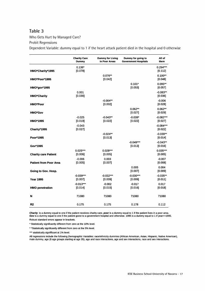
The probit coefficients are presented in the first column of Table 3. In order to control for robustness we also ran the OLS specification, and we also instrumented HMO penetration by the average firm size of the MSA. The coefficients obtained are consistent with the probit ones. Finally, we also ran the same specifications including only those patients who suffered from a heart attack and stayed in the hospital for five days or fewer. The results are robust and presented at Table A.2 in the Appendix. The results are consistent and show a positive effect of HMO penetration on the probability of dying of heart attack for the uninsured.

The probit results in Table 1.9 imply that a charity care patient in 1995 from an MSA that had the average HMO penetration of 0.398 would have a 3.6% higher probability of dying than an insured patient. If the HMO enrollment had been one standard deviation lower, a charity care patient in 1995 would have had a probability of dying of a heart attack 2% higher than an insured patient. These are considerable numbers if we take into account that the average probability of dying of a heart attack in 1995 was 11.8%. The charity care dummy is significantly positive, indicating that the uninsured have a higher probability of dying after a heart attack. Also, the year 1995 dummy is significantly negative, reflecting the improvement in medical technology during the decade under consideration, which has allowed the probability of dying of heart attack to decrease from 15.2% in 1985 to 11.8% in 1995.

These results confirm the fact that HMO penetration has a negative impact on the health of the uninsured. However, the negative impact could be due to their worse access to care or also to the fact that they now go to government hospitals, which in turn have worse quality. Hence, if these are the mechanisms by which managed care leads to worse health outcomes, not only the uninsured, but also those living in poor areas and those going to government hospitals, can suffer worse health.

9 I only include these patients who are 35 or older because there are almost no cases of heart attack for younger patients. I consider nine different age groups (pre-determined by my data):35-44 years old, 45-54, 55-59, 60-64, 65-69, 70-74, 75-79, 80-84, and 85 or older.


In order to analyze if managed care also affects the health of the people living in poor areas, I use the following specification:

msazipiiitmsa

tmsamsatmsamsatmsazipmsai

ZIPDEMMSAPHMO

HMOPHMOPHMOdied

,,,

,,,,,

1995

1995**1995**


++++++∆+

+∆+∆+∆=

where P is a dummy variable equal to one if the patient lives in a poor are (an area whose average income per capita is below the thirty-third percentile level for California). The rest of the variables are defined as before.

The second column in Table 3 presents the probit coefficients. The OLS coefficients and the instrumental variables specification as well as the results including only these patients staying in the hospital for five days or fewer are robust and are included in Table A.3 in the Appendix. The probit coefficients imply that a patient who lived in a poor neighborhood in 1995 in an MSA that had the average HMO penetration of 0.398 would have a 0.8% higher probability of dying than a patient living in a non-poor area. However, if the HMO penetration had been one standard deviation lower instead, a patient living in a poor neighborhood in 1995 would have had almost the same probability of dying (0.1% lower) as a patient living in a rich area. The charity care dummy is significantly positive, indicating that the uninsured have a 2.8% higher probability of dying after a heart attack than the insured. Again, the year dummy for 1995 is significantly negative, reflecting the medical improvements for heart attack treatment during the decade under consideration.

Another reason for managed care penetration leading to worse health outcomes for the uninsured could be the fact that, with the increase in price competition, charity care patients shift to government hospitals (Table 1), which in turn experience a worsening of their quality in areas where managed care penetration is stronger (Table 2). If this is the case, then we should expect managed care to affect all the patients who are treated in government hospitals independently of their insurance status. In order to test if this is the case, we use the following specification:

where G corresponds to a dummy variable that is one if the patient goes to a government hospital and zero otherwise. The rest of the variables are defined as previously indicated.

The third column in Table 3 presents the probit results. The OLS and instrumental variables specification are included in Table A.4 in the Appendix. The coefficients from the probit imply that a person going to a government hospital in 1995 after suffering a heart attack (and using the average HMO penetration for 1995 in California) had a 2.1% higher probability of dying than those patients going to other kinds of hospitals. A one standard deviation lower HMO penetration would mean only a 0.1% higher probability of dying for these going to government hospitals compared to patients who go to other hospital types. This effect remains more severe for the charity care patients.

Hence, managed care penetration has a negative impact on the three groups of patients: those living in poor areas, the uninsured and patients going to government hospitals. However, these groups are not mutually exclusive. It could be the case that we observe a worsening of the health outcomes of those going to government hospitals, just because most of them are poor

msazipiihtmsa

tmsahtmsahtmsazipmsahi

ZIPDEMMSAGHMO

HMOGHMOGHMOdied

,,,

,,,,,,

1995

1995**1995**


++++++∆+

+∆+∆+∆=


and what we am picking up is the impact of managed care penetration on the health of the poor. A similar reasoning could be made for the uninsured.

In order to determine which of the groups is affected by managed care penetration, in the final specification we include all three interactions with managed care penetration. The probit results are presented in the last column of Table 3. The coefficients for HMO*charity*1995, HMO*poor*1995 and HMO*gov*1995 are all positive and significant. Taking into account all the relevant coefficients, a charity care patient in 1995 in an MSA with the average 1995 HMO penetration has a 3.3% higher probability of dying than an insured patient. A patient who goes to a government hospital has a 2.5% higher probability of dying than somebody who goes to another type of hospital. However, people who live in poor areas have almost the same probability of dying (0.08% lower) as people living in other neighborhoods, after controlling for being uninsured and going to government hospitals.

Hence, regarding the effect of managed care penetration on health outcomes – as measured by their probability of dying after a heart attack – we can conclude that managed care has a negative impact on the health care outcomes of charity care patients and those who go to government hospitals. Our results also indicate that the impact on the health of those living in poor areas, after controlling for their insurance status and the kind of hospital they go to, is negligible.

V. Conclusions Managed care penetration has often been blamed for increasing financial pressures on hospitals and some previous work has confirmed that HMO enrollment had a particularly negative effect for the survival of the safety net hospitals and also for the provision of the type of services most commonly used by the uninsured.

Our goal in this paper is to test whether managed care has also had any effect on the health of the uninsured population.

Our findings help us understand the path through which managed care can have a negative effect on the health of the uninsured: its financial pressures encourage charity care patients to concentrate in public hospitals. Those, in turn, face the challenge of providing health care to a higher proportion of non-paying patients. Our results hint towards the possibility of a trade-off between hospitals’ quantity of non-paying charity care and the quality of the care they provide.

Finally, regarding the effect of managed care penetration in health outcomes – as measured by patients’ probability of dying after a heart attack – we can conclude that managed care has a negative impact on the health care outcomes of charity care patients and those who go to government hospitals.

These results bring a new perspective to managed care. Its impact on American health should be analyzed beyond the efficiency implications and more research should be conducted regarding its effects on the overall health care market.


Referencias American College of Physicians-American Society of Internal Medicine (2000) “No Health

Insurance? It’s enough to Make you Sick,” Philadelphia, American College of Physicians-American Society of Internal Medicine.

American Hospital Association (1986), “Cost and Compassion: Recommendations for Avoiding a Crisis in Care for the Medically Indigent,” Chicago.

Aaron, H. (1991), “Serious and Unstable condition: Financing America´s Health Care,” Washington D.D., Brookings Institution.

Baker, L. (1999), “Association of managed care market share and health expenditure for fee-for-service Medicare patients,” Journal of the American Medical Association, pp. 432-437.

Baker, L. and S. Shankarkumar (1997), “Managed Care and Health Care Expenditures: Evidence from Medicare, 1990-1994,” NBER Working Paper 6187.

Currie, J. and J. Fahr (2004), “Hospitals, managed care and the charity caseload in California,” Journal of Health Economics, 23 (3), pp. 421-442.

Currie J. and P. Reagan (1998), “Distance to hospital and children’s access to care: is being closer better, and for whom?,” NBER Working Paper 6836.

Cutler, D. (1995), “The Cost and Financing of Health Care,” American Economic Review, 85(2), pp. 32-37.

Cutler, D. and J. Barro (1997), “Consolidation in the Medical care Marketplace: a Case Study for Massachusetts,” NBER Working Paper 5957.

Duke, K. (1996), “Hospitals in a changing healthcare system,” Health Affairs, 15(2), pp. 49-61.

Frank, R and D. Salkever (1991), “The Supply of Charity Services by nonprofit hospitals: motives and market structure,” RAND Journal of Economics, 22(3), pp. 430-445.

Frank, R. et al. (1990), “Market forces and the public good. Competition among hospitals and provision of indigent care,” Advances in Health Economics and Health Services Research, 11, pp. 159-183.

Kaiser (2008), “The Uninsured: A Primer,” The Kaiser Commission on Medicaid and the Uninsured, October, 2008.

McClellan, M. and D. Staiger (2000), “Comparing Quality at For-Profit and Not-For-Profit Hospitals,” The Changing Hospital Industry, Comparing Not-for-profit and For-profit Institutions, NBER.

Mas, N. (2009), “Responding to financial pressures. The effect of managed care on hospital´s provision of charity care,” IESE WP 782.

Mas, N. and J. Seinfeld (2008), “Is Managed care restraining the adoption of technology by hospitals?,” Journal of Health Economics, 27, pp. 1026-1045.

Richardson, E. (1999), “Managed Care and Access to Care by the Poor,” mimeo.

Thorpe, K.E. and C.E. Phelps (1991), “The social role of not-for-profit organizations: hospital provision of charity care,” Economic Inquiry, 29(3), pp. 472-484.


Table 1 Managed Care Effects on the Provision of Charity Care in California

DEPENDENT VARIABLES Ch%MSA UC Provided Ch%MSA MCal Provided Ch.%MSA UC&MCal Provided

[1] [2] [3]

HMO change -0,005** 0,004 -0,003**[0,001] [0,003] [0,001]

HMO change*poor 0,0595 1,406 0,533[0,195] [1,295] [0,496]

HMO change*teaching 0,326** 0,096 -0,002[0,098] [0,774] [0,404]

HMO change * gov 4.140* 6,230* 2,501*[2.644] [3,334] [1.330]

Poor 0,695 -6,151 -3,152[0,888] [3,962] [3,014]

Teaching -0,928* -10,701* -4,833*[0,518] [6,075] [2,562]

Government -0,122 -3,461** -1,346[0,321] [1,485] [1,002]

Only hospital -1,010** -2,746 -1,726*[0,462] [1,754] [1,070]

Only hospital*poor 0,069 7,957* 4,171[1,109] [4,694] [3,352]

Only hospital*Teaching 1,104 3,028 4,393[1.554] [6,946] [3,097]

Only hospital*gov 0,371 9.211** 1,653[1.353] [4.240] [1,834]

Demographics yes yes yesHospital Characteristics yes yes yesN 210 210 210R2 0,202 0,271 0,292

UC refers to uncompensated care and Mcal to Medi-Cal.

Robust standard errors appear in brackets.

* Statistically significantly different from zero at the 10% level.

* *Statistically significantly different from zero at the 5% level.

DEPENDENT VARIABLES Ch%MSA UC Provided Ch%MSA MCal Provided Ch.%MSA UC&MCal Provided DEPENDENT VARIABLES Ch%MSA UC Provided Ch%MSA MCal Provided Ch.%MSA UC&MCal Provided

[1] [2] [3]

HMO change -0,005** 0,004 -0,003**[0,001] [0,003] [0,001]

HMO change*poor 0,0595 1,406 0,533[0,195] [1,295] [0,496]

HMO change*teaching 0,326** 0,096 -0,002[0,098] [0,774] [0,404]

HMO change * gov 4.140* 6,230* 2,501*[2.644] [3,334] [1.330]

Poor 0,695 -6,151 -3,152[0,888] [3,962] [3,014]

Teaching -0,928* -10,701* -4,833*[0,518] [6,075] [2,562]

Government -0,122 -3,461** -1,346[0,321] [1,485] [1,002]

Only hospital -1,010** -2,746 -1,726*[0,462] [1,754] [1,070]

Only hospital*poor 0,069 7,957* 4,171[1,109] [4,694] [3,352]

Only hospital*Teaching 1,104 3,028 4,393[1.554] [6,946] [3,097]

Only hospital*gov 0,371 9.211** 1,653[1.353] [4.240] [1,834]

Demographics yes yes yesHospital Characteristics yes yes yesN 210 210 210R2 0,202 0,271 0,292






Table 2 Managed Care Effects on Quality for California Dependent Variable: Change in the Proportion of Patients with Heart Attack that Died

Withunit

Hosps cardiac

intensive Withunit

[1] [2] [3] [4] [1b] [2b] [3b] [4b]

length of stay <6 days

HMO Change -7,240** -2,64* -2,140* -2,400 -1,580 -1,528 -1,691 -4,651

[3,82] [1,571] [1,280] [2,780] [1,410] [2,315] [2,330] [5,131]

HMO change*poor 0,016 0,055 0,030* -0,048 0,083 0,229 -0,091* 0,022

[0,021] [0,115] [0,017] [0,075] [0,085] [0,364] [0,030] [0,175]

HMO change*teaching -0,007 0,271 0,011 -0,060 0,045 0,820 0,0811* 0,211

[0,018] [0,180] [0,030] [0,127] [0,064] [0,692] [0,049] [0,252]

HMO change * gov 2,421* 8,280* 3,246* 1,46** 6,471* 3,009* 8,341** 9,263*

[1,310] [4,840] [1,728] [0,635] [3,898] [1,749] [2,614] [5,293]

Poor -0,209** -0,309 -0,163** -0,108 -0,212 -0,573 0,011 -0,132

[0,063] [0,210] [0,059] [0,106] [0,168] 0,687 [0,113] [0,257]

Teaching -0,237** -0,552** -0,192** -0,132* -0,638** -1,578* -0,525** -0,501**

[0,081] [0,206] [0,070] [0,077] [0,218] [0,963] [0,124] [0,132]

Government 0,044 -2,63 -0,084 -0,279** 0,492 -0,312 -0,048 -0,231[0,130] [0,233] [0,054] [0,102] [0,618] [0,687] [0,090] [0,177]

Only hospital -0,272 -0,166 -0,373** -0,526** 0,138 -0,238 -0,358 -0,554*

[0,383] [0,260] [0,108] [0,133] [0,440] [0,538] [0,267] [0,296]

Only hospital*poor 0,233 0,539 0,449** 0,417** 0,311 0,885 0,469* 0,716

[0,357] [0,385] [0,121] [0,186] [0,470] [1,150] [0,280] [0,451]

Only hospital*Teaching -0,298 -0,113 -0,190 -0,435 0,142 0,807 0,824** 0,398

[0,379] [0,518] [0,329] [0,362] [0,932] [4,401] [0,378] [0,562]

Only hospital*gov 0,286 0,265 0,527** 0,978** 1,019 -0,461 -0,086 0,406

[0,490] [0,505] [0,329] [0,338] [0,996] [1,108] [0,450] [0,569]

Demographic Characteristics yes yes yes yes yes yes yes yes

Hospital Characteristics yes yes yes yes yes yes yes yes

N 210 210 166 166 209 209 166 166

R2 0,166 0,238 0,288 0,183 0,370 0,319 0,298 0,199

(1) Includes all urban hospitals in California.

(2) The same as (1) instrumenting HMO penetration by average firm size in the MSA.

(3) FOR HOSPITAL WITH CARDIAC INTENSIVE CARE.


[1b],[2b],[3b] and [4b] The same as (1), (2), (3) and(4) limiting the sample to these patients that stay at the hospital five or less days.




Hosps cardiac

intensive Withunit

Hosps cardiac

intensive Withunit

[1] [2] [3] [4] [1b] [2b] [3b] [4b]

length of stay <6 days

HMO Change -7,240** -2,64* -2,140* -2,400 -1,580 -1,528 -1,691 -4,651

[3,82] [1,571] [1,280] [2,780] [1,410] [2,315] [2,330] [5,131]

HMO change*poor 0,016 0,055 0,030* -0,048 0,083 0,229 -0,091* 0,022

[0,021] [0,115] [0,017] [0,075] [0,085] [0,364] [0,030] [0,175]

HMO change*teaching -0,007 0,271 0,011 -0,060 0,045 0,820 0,0811* 0,211

[0,018] [0,180] [0,030] [0,127] [0,064] [0,692] [0,049] [0,252]

HMO change * gov 2,421* 8,280* 3,246* 1,46** 6,471* 3,009* 8,341** 9,263*

[1,310] [4,840] [1,728] [0,635] [3,898] [1,749] [2,614] [5,293]

Poor -0,209** -0,309 -0,163** -0,108 -0,212 -0,573 0,011 -0,132

[0,063] [0,210] [0,059] [0,106] [0,168] 0,687 [0,113] [0,257]

Teaching -0,237** -0,552** -0,192** -0,132* -0,638** -1,578* -0,525** -0,501**

[0,081] [0,206] [0,070] [0,077] [0,218] [0,963] [0,124] [0,132]

Government 0,044 -2,63 -0,084 -0,279** 0,492 -0,312 -0,048 -0,231[0,130] [0,233] [0,054] [0,102] [0,618] [0,687] [0,090] [0,177]

Only hospital -0,272 -0,166 -0,373** -0,526** 0,138 -0,238 -0,358 -0,554*

[0,383] [0,260] [0,108] [0,133] [0,440] [0,538] [0,267] [0,296]

Only hospital*poor 0,233 0,539 0,449** 0,417** 0,311 0,885 0,469* 0,716

[0,357] [0,385] [0,121] [0,186] [0,470] [1,150] [0,280] [0,451]

Only hospital*Teaching -0,298 -0,113 -0,190 -0,435 0,142 0,807 0,824** 0,398

[0,379] [0,518] [0,329] [0,362] [0,932] [4,401] [0,378] [0,562]

Only hospital*gov 0,286 0,265 0,527** 0,978** 1,019 -0,461 -0,086 0,406

[0,490] [0,505] [0,329] [0,338] [0,996] [1,108] [0,450] [0,569]

Demographic Characteristics yes yes yes yes yes yes yes yes

Hospital Characteristics yes yes yes yes yes yes yes yes

N 210 210 166 166 209 209 166 166

R2 0,166 0,238 0,288 0,183 0,370 0,319 0,298 0,199

(1) Includes all urban hospitals in California.


(3) FOR HOSPITAL WITH CARDIAC INTENSIVE CARE.


[1b],[2b],[3b] and [4b] The same as (1), (2), (3) and(4) limiting the sample to these patients that stay at the hospital five or less days.




Hosps cardiac

intensive


Table 3 Who Gets Hurt by Managed Care? Probit Regressions Dependent Variable: dummy equal to 1 if the heart attack patient died in the hospital and 0 otherwise




*** statistically signifficant at 1% level.

All regressions include the following Demographic Variables: race/ethnicity dummies (African American, Asian, Hispanic, Native American),male dummy, age (8 age groups starting at age 35), age and race interactions, age and sex interactions, race and sex interactions.

Charity is a dummy equal to one if the patient receives charity care, poor is a dummy equal to 1 if the patient lives in a poor area.Gov is a dummy equal to one if the patient goest to a government hospital and otherwise. 1995 is a dummy equal to 1 if year==1995.

Charity CareDummy

Dummy for Livingin Poor Areas

Dummy for going toGovernment Hospitals

All ofthem

HMO*Charity*19950.136*[0.078]

0.294***[0.112]

HMO*Poor*19950.076**[0.042]

0.100**[0.048]

HMO*gov*19950.101*[0.053]

0.095**[0.057]

HMO*Charity0.001

[0.030]-0.083**[0.036]

HMO*Poor-0.004**[0.002]

-0.006[0.028]

HMO*Gov0.062**[0.027]

0.062**[0.029]

HMO*1995-0.025[0.019]

-0.043**[0.022]

-0.039*[0.022]

-0.082***[0.027]

Charity*1995-0.043[0.027]

-0.084***[0.022]

Poor*1995-0.024**[0.013]

-0.039**[0.014]

Gov*1995-0.049***[0.013]

-0.043**[0.016]

Charity care Patient0.025***[0.006]

0.028***[0.005]

0.035***[0.005]

Patient from Poor Area-0.006[0.005]

0.003[0.007]

-0.007[0.008]

Going to Gov. Hosp.0.005

[0.007]0.004

[0.009]

Year 1995-0.039***[0.007]

-0.032***[0.009]

-0.030***[0.009]

-0.035**[0.011]

HMO penetration-0.013***[0.014]

-0.002[0.015]

-0.017[0.016]

0.017[0.018]

N 71080 71080 71080 71080

R2 0.175 0.175 0.178 0.112






Charity is a dummy equal to one if the patient receives charity care, poor is a dummy equal to 1 if the patient lives in a poor area.Gov is a dummy equal to one if the patient goest to a government hospital and otherwise. 1995 is a dummy equal to 1 if year==1995.

Charity CareDummy

Dummy for Livingin Poor Areas

Dummy for going toGovernment Hospitals

All ofthem

HMO*Charity*19950.136*[0.078]

0.294***[0.112]

HMO*Poor*19950.076**[0.042]

0.100**[0.048]

HMO*gov*19950.101*[0.053]

0.095**[0.057]

HMO*Charity0.001

[0.030]-0.083**[0.036]

HMO*Poor-0.004**[0.002]

-0.006[0.028]

HMO*Gov0.062**[0.027]

0.062**[0.029]

HMO*1995-0.025[0.019]

-0.043**[0.022]

-0.039*[0.022]

-0.082***[0.027]

Charity*1995-0.043[0.027]

-0.084***[0.022]

Poor*1995-0.024**[0.013]

-0.039**[0.014]

Gov*1995-0.049***[0.013]

-0.043**[0.016]

Charity care Patient0.025***[0.006]

0.028***[0.005]

0.035***[0.005]

Patient from Poor Area-0.006[0.005]

0.003[0.007]

-0.007[0.008]

Going to Gov. Hosp.0.005

[0.007]0.004

[0.009]

Year 1995-0.039***[0.007]

-0.032***[0.009]

-0.030***[0.009]

-0.035**[0.011]

HMO penetration-0.013***[0.014]

-0.002[0.015]

-0.017[0.016]

0.017[0.018]

N 71080 71080 71080 71080

R2 0.175 0.175 0.178 0.112


Appendix Table A.1 Managed Care Effects on the Provision of Charity Care in California Instrumental Variables


[1] [2] [3]

HMO change -0,015* 0,102 -0,045*[0,009] [0,123] [0,026]

HMO change*poor 0,979 -0,423 -0,331[0,688] [1,594] [1,253]

HMO change*teaching 1,339* 0,198 0,587[0,765] [0,730] [0,529]

HMO change * gov 3,750* 2,136* 1,959**[2,045] [1,186] [0,980]

Poor -0,592 -2,453 -1,440[1,018] [2,993] [1,356]

Teaching -1,410 -9,491* -4,838[0,805] [5,752] [2,680]

Government 0,530 1,128 0,660[1,312] [0,970] [0,716]

Only hospital -0,976 0,144 -0,429[0,591] [0,699] [0,513]

Only hospital*poor 2,057 1,714 1,271[1,649] [3,213] [1,316]

Only hospital*Teaching 1,548 2,619 4,529[2,451] [7,229] [3,129]

Only hospital*gov -0,615 3,746 -0,833[2,374] [4,518] [1,679]

Demographics yes yes yes

Hospital Characteristics yes yes yes

N 210 210 210

R2 0,193 0,139 0,184



Managed care enrollment has been instrumented by firm size.

* Statistically significantly different from zero at the 10% level. * *Statistically significantly different from zero at the 5% level.


[1] [2] [3]

HMO change -0,015* 0,102 -0,045*[0,009] [0,123] [0,026]

HMO change*poor 0,979 -0,423 -0,331[0,688] [1,594] [1,253]

HMO change*teaching 1,339* 0,198 0,587[0,765] [0,730] [0,529]

HMO change * gov 3,750* 2,136* 1,959**[2,045] [1,186] [0,980]

Poor -0,592 -2,453 -1,440[1,018] [2,993] [1,356]

Teaching -1,410 -9,491* -4,838[0,805] [5,752] [2,680]

Government 0,530 1,128 0,660[1,312] [0,970] [0,716]

Only hospital -0,976 0,144 -0,429[0,591] [0,699] [0,513]

Only hospital*poor 2,057 1,714 1,271[1,649] [3,213] [1,316]

Only hospital*Teaching 1,548 2,619 4,529[2,451] [7,229] [3,129]

Only hospital*gov -0,615 3,746 -0,833[2,374] [4,518] [1,679]

Demographics yes yes yes

Hospital Characteristics yes yes yes

N 210 210 210

R2 0,193 0,139 0,184



Managed care enrollment has been instrumented by firm size.

* Statistically significantly different from zero at the 10% level. * *Statistically significantly different from zero at the 5% level.


Appendix (continued) Table A.2 Impact of HMO Penetration on the Uninsured’s Health Dependent Variable: Change in the Proportion of Patients with Heart Attack that Died

Length of stay<6 days

[1] [2] [3] [1b] [2b] [3b]

HMO*Charity*1995 0.117* 0.235*** 0.136* 0.358*** 0.441*** 0.258*

[0.060] [0.074] [0.078] [0.073] [0.092] [0.141]

HMO*Charity -0,006 -0.086*** 0,001 -0.281*** -0.390*** -0.184***

[0.026] [0.028] [0.030] [0.042] [0.046] [0.047]

HMO*1995 -0,012 -0.094** -0,025 -0.062* -0.154* -0.095***

[0.020] [0.046] [0.019] [0.031] [0.080] [0.029]

Charity*1995 -0,028 -0.076** -0,043 0,016 -0,020 -0,015

[0.022] [0.029] [0.027] [0.026] [0.036] [0.052]

Charity care 0.019*** 0.018** 0.025*** 0.014* 0.040** 0.029***

[0.005] [0.006] [0.006] [0.008] [0.009] [0.009]

Year 1995 -0.046*** 0,022 -0.039*** -0.209*** -0.095* -0.185***

[0.008] [0.030] [0.007] [0.011] [0.051] [0.014]

HMO penetration -0,014 -0.138* -0,013 0,032 -0.348** 0,030

[0.015] [0.075] [0.014] [0.028] [0.128] [0.022]

Poor -0,007 -0,010 -0,006 -0,005 -0,009 -0,003

[0.005] [0.006] [0.005] [0.007] [0.009] [0.007]

N 71080 71080 71080 34784 34784 34784R2 0,331 0,334 0,175 0,353 0,365 0,185

Charity is a dummy equal to one if the patient receives charity care, poor is a dummy equal to 1 if the patient lives in a poor area.

(1) OLS regression, (2) with IV instrumenting HMO penetration by firm size, (3) probit. (1)b, (2)b, (3)b are the same regressions butincluding only these patients that stay in the hospital five days or less.

1995 is a dummy equal to 1 if year==1995 and 0 if year==1985.






All regressions include the following Zip Variables: percentage in poverty, percentage unemployed, percentage with high school or more,population. The following MSA variables are also included: HMO penetration, MCR penetration, MCD penetration and percentage of uninsured.

For the previous MSA variables I included both their level in 1985 and the change berween 1985 and 1995.


[1] [2] [3] [1b] [2b] [3b]

HMO*Charity*1995 0.117* 0.235*** 0.136* 0.358*** 0.441*** 0.258*

[0.060] [0.074] [0.078] [0.073] [0.092] [0.141]

HMO*Charity -0,006 -0.086*** 0,001 -0.281*** -0.390*** -0.184***

[0.026] [0.028] [0.030] [0.042] [0.046] [0.047]

HMO*1995 -0,012 -0.094** -0,025 -0.062* -0.154* -0.095***

[0.020] [0.046] [0.019] [0.031] [0.080] [0.029]

Charity*1995 -0,028 -0.076** -0,043 0,016 -0,020 -0,015

[0.022] [0.029] [0.027] [0.026] [0.036] [0.052]

Charity care 0.019*** 0.018** 0.025*** 0.014* 0.040** 0.029***

[0.005] [0.006] [0.006] [0.008] [0.009] [0.009]

Year 1995 -0.046*** 0,022 -0.039*** -0.209*** -0.095* -0.185***

[0.008] [0.030] [0.007] [0.011] [0.051] [0.014]

HMO penetration -0,014 -0.138* -0,013 0,032 -0.348** 0,030

[0.015] [0.075] [0.014] [0.028] [0.128] [0.022]

Poor -0,007 -0,010 -0,006 -0,005 -0,009 -0,003

[0.005] [0.006] [0.005] [0.007] [0.009] [0.007]

N 71080 71080 71080 34784 34784 34784R2 0,331 0,334 0,175 0,353 0,365 0,185












Appendix (continued) Table A.3 Impact of HMO Penetration on the Health of Heart Attack Patients Living in Poor Neighborhoods Dependent Variable: dummy equal to 1 if the heart attack patient died in the hospital and 0 otherwise


[1] [2] [3] [1b] [2b] [3b]

HMO*poor*1995 0.070* 0.159** 0.076** 0,030 0,105 0,057

[0.042] [0.063] [0.042] [0.068] [0.108] [0.065]

HMO*poor -0,041 -0,068 -0.004** -0,029 -0,006 -0,025

[0.027] [0.043] [0.002] [0.056] [0.093] [0.040]

HMO*1995 -0,029 -0.118** -0.043** -0,048 -0,131 -0.098**

[0.023] [0.050] [0.022] [0.035] [0.087] [0.033]

Poor*1995 -0,024 -0.068*** -0.024** -0,014 -0,057 -0,017

[0.015] [0.025] [0.013] [0.022] [0.038] [0.021]

Poor neighborhood 0,003 0,014 0,003 0,005 0,002 0,002

[0.007] [0.013] [0.007] [0.014] [0.028] [0.011]

Year 1995 -0.039*** -0,032 -0.032*** -0.203*** -0.098* -0.179***

[0.009] [0.032] [0.009] [0.013] [0.054] [0.016]

HMO penetration -0,003 -0,106 -0,002 0,020 -0,031 0,027

[0.017] [0.078] [0.015] [0.031] [0.132] [0.024]

Charity Care Patient 0.022*** 0.028*** 0.028*** 0.009* 0.071*** 0.013**

[0.004] [0.004] [0.005] [0.006] [0.007] [0.007]

N 71080 71080 71080 34784 34784 34784R2 0,331 0,324 0,175 0,353 0,365 0,185












[1] [2] [3] [1b] [2b] [3b]

HMO*poor*1995 0.070* 0.159** 0.076** 0,030 0,105 0,057

[0.042] [0.063] [0.042] [0.068] [0.108] [0.065]

HMO*poor -0,041 -0,068 -0.004** -0,029 -0,006 -0,025

[0.027] [0.043] [0.002] [0.056] [0.093] [0.040]

HMO*1995 -0,029 -0.118** -0.043** -0,048 -0,131 -0.098**

[0.023] [0.050] [0.022] [0.035] [0.087] [0.033]

Poor*1995 -0,024 -0.068*** -0.024** -0,014 -0,057 -0,017

[0.015] [0.025] [0.013] [0.022] [0.038] [0.021]

Poor neighborhood 0,003 0,014 0,003 0,005 0,002 0,002

[0.007] [0.013] [0.007] [0.014] [0.028] [0.011]

Year 1995 -0.039*** -0,032 -0.032*** -0.203*** -0.098* -0.179***

[0.009] [0.032] [0.009] [0.013] [0.054] [0.016]

HMO penetration -0,003 -0,106 -0,002 0,020 -0,031 0,027

[0.017] [0.078] [0.015] [0.031] [0.132] [0.024]

Charity Care Patient 0.022*** 0.028*** 0.028*** 0.009* 0.071*** 0.013**

[0.004] [0.004] [0.005] [0.006] [0.007] [0.007]

N 71080 71080 71080 34784 34784 34784R2 0,331 0,324 0,175 0,353 0,365 0,185












Appendix (continued) Table A.4 Impact of HMO Penetration on Probability of Dying from Heart Attack Patients Goint to Government Hospitals Dependent Variable: dummy equal to 1 if the patient died in the hospital and 0 otherwise


[1] [2] [3] [1b] [2b] [3b]

HMO*Gov*1995 0.093* 0.224** 0.101* 0.131* 0,008 0.123*

[0.053] [0.077] [0.053] [0.080] [0.124] [0.070]

HMO*Gov hospital 0.061* 0,015 0.062** 0,019 0,123 0,044

[0.031] [0.050] [0.027] [0.062] [0.099] [0.044]

HMO*1995 -0,026 -0.131** -0.039* -0,056 -0,136 -0.096**

[0.023] [0.050] [0.022] [0.037] [0.088] [0.034]

Gov Hospital*1995 -0.055** -0.113*** -0.049*** -0.053* -0,009 -0.048*

[0.019] [0.030] [0.013] [0.027] [0.046] [0.022]

Gov hospital 0,007 0,021 0,005 0,009 -0,026 0,004

[0.009] [0.018] [0.007] [0.017] [0.033] [0.012]

Year 1995 -0.036*** -0,038 -0.030*** -0.203*** -0.095* -0.182***

[0.009] [0.033] [0.009] [0.013] [0.056] [0.016]

HMO penetration -0,018 -0,107 -0,017 0,016 -0,348 0,020

[0.017] [0.084] [0.016] [0.033] [0.244] [0.026]

Charity Care Patient 0.016*** 0.034*** 0.019*** 0,001 0.078*** 0,004

[0.004] [0.005] [0.005] [0.006] [0.007] [0.008]

Poor -0,005 -0,006 -0,004 -0,001 -0,0002 0,001

[0.005] [0.006] [0.005] [0.07] [0.010] [0.007]

N 61519 61519 61519 29991 29991 29991

R2 0,153 0,114 0,175 0,161 0,123 0,183

Gov is a dummy equal to one if the patient went to a government hospital. Charity is a dummy equal to one if the patient receivescharity care, poor is a dummy equal to 1 if the patient lives in a poor area.(1) OLS regression, (2) with IV instrumenting HMO penetration by firm size, (3) probit. (1)b, (2)b, (3)b are the same regressions butincluding only these patients that stay in the hospital five days or less.










[1] [2] [3] [1b] [2b] [3b]

HMO*Gov*1995 0.093* 0.224** 0.101* 0.131* 0,008 0.123*

[0.053] [0.077] [0.053] [0.080] [0.124] [0.070]

HMO*Gov hospital 0.061* 0,015 0.062** 0,019 0,123 0,044

[0.031] [0.050] [0.027] [0.062] [0.099] [0.044]

HMO*1995 -0,026 -0.131** -0.039* -0,056 -0,136 -0.096**

[0.023] [0.050] [0.022] [0.037] [0.088] [0.034]

Gov Hospital*1995 -0.055** -0.113*** -0.049*** -0.053* -0,009 -0.048*

[0.019] [0.030] [0.013] [0.027] [0.046] [0.022]

Gov hospital 0,007 0,021 0,005 0,009 -0,026 0,004

[0.009] [0.018] [0.007] [0.017] [0.033] [0.012]

Year 1995 -0.036*** -0,038 -0.030*** -0.203*** -0.095* -0.182***

[0.009] [0.033] [0.009] [0.013] [0.056] [0.016]

HMO penetration -0,018 -0,107 -0,017 0,016 -0,348 0,020

[0.017] [0.084] [0.016] [0.033] [0.244] [0.026]

Charity Care Patient 0.016*** 0.034*** 0.019*** 0,001 0.078*** 0,004

[0.004] [0.005] [0.005] [0.006] [0.007] [0.008]

Poor -0,005 -0,006 -0,004 -0,001 -0,0002 0,001

[0.005] [0.006] [0.005] [0.07] [0.010] [0.007]

N 61519 61519 61519 29991 29991 29991

R2 0,153 0,114 0,175 0,161 0,123 0,183

Gov is a dummy equal to one if the patient went to a government hospital. Charity is a dummy equal to one if the patient receivescharity care, poor is a dummy equal to 1 if the patient lives in a poor area.(1) OLS regression, (2) with IV instrumenting HMO penetration by firm size, (3) probit. (1)b, (2)b, (3)b are the same regressions butincluding only these patients that stay in the hospital five days or less.









hospital financial pressures and the health … · the sponsors of the sp-sp center are the ......

Documents