1

Hot money in bank credit flows to emerging markets during the banking globalization era

Ana-Maria Fuertes, Kate Phylaktis, Cheng Yan*

September 28, 2014

Abstract

This paper investigates the relative importance of hot money in bank credit and portfolio flows from the US to 18 emerging markets over the period 1988-2012. We deploy state-space models à la Kalman filter to identify the unobserved hot money as the temporary component of each type of flow. The analysis reveals that the importance of hot money relative to the permanent component in bank credit flows has significantly increased during the 2000s relative to the 1990s. This finding is robust to controlling for the influence of push and pull factors in the two unobserved components. The evidence supports indirectly the view that global banks have played an important role in the transmission of the global financial crisis to emerging markets, and endorses the use of regulations to manage international capital flows.

Keywords: International capital flows; Hot money; Crisis transmission; Banking globalisation; Kalman filter.

JEL classification: E44; F20; F34; G1.

* Corresponding author: Kate Phylaktis, k.phylaktis@city.ac.uk. Cass Business School, City University

London , 106 Bunhill Row, London EC1Y 8TZ4; A.Fuertes@city.ac.uk; Cheng Yan.1@cass.city.uk.

2

“When one region of the world economy experiences a financial crisis, the world-wide availability of investment opportunities declines. As global investors search for new destinations for their capital, other regions will experience inflows of hot money. However, large capital inflows make the recipient countries more vulnerable to future adverse shocks, creating the risk of serial financial crises.” (Korinek, 2011)

1. Introduction

International capital flows increased dramatically in the 1990s and it has been argued that

they eventually led to the 1997 Asian Financial Crisis (Kaminsky and Reinhart 1998;

Kaminsky, 1999; Chari and Kehoe, 2003). International capital flows resurged again until the

late 2000s Global Financial Crisis (GFC). Global capital flows increased rapidly from less

than 7% of world GDP in 1998 to over 20% in 2007, but suffer large reversals in late 2008,

with bank credit flows being hit the hardest (Milesi-Ferretti and Tille, 2011; Tong and Wei,

2011; Forbes and Warnock, 2012). Is this reversal of global capital flows due to hot money?

The term hot money has been most commonly used for capital moving from one country

to another in order to earn a short-term profit on interest rate differentials or anticipated

exchange rate shifts. This speculative capital can lead to market instability (Martin and

Morrison, 2008; Chari and Kehoe, 2003). 1 Recently, the equity premium has been suggested

as a driver of hot money (Guo and Huang, 2010). Instead of ascertaining driving factors,

some studies have sought to identify hot money via the unobserved-component models by

focusing on its temporariness and reversibility aspects (see, e.g, Sarno and Taylor, 1999a, b).

A surge in hot money to emerging markets (EMs) may be destabilizing and trigger

regulation, of which examples abound since 2009 such as Brazil, Taiwan, South Korea,

Indonesia and Thailand among other countries. Thus, measuring hot money becomes crucial

for appropriate policy design (IMF, 2011; Ostry et al., 2010; McCauley 2010; Korinek, 2011).

It is well known that distinct types of capital flows have distinct degrees of reversibility

(Tong and Wei, 2011; Sarno and Taylor, 1999a).2 In fact, a key feature of the post-1990s

1 Huge movements of hot money have been historically not atypical in fixed exchange rate systems (e.g., during the final years of the Bretton Woods system). Recently, there is a growing interest on carry trade, seen as a type of hot money (McKinnon and Schnabl, 2009; McCauley, 2010; McKinnon, 2013; McKinnon and Liu, 2013). 2 It is usually referred as the composition hypothesis. The rationale is that a more volatile form of capital will be more likely to fly out of the country in crisis. Tong and Wei (2011) do not find a connection between a country’s

3

trend in capital flows to EMs up until the GFC is the dramatic resurgence of international

bank credit flows relative to equity and bond flows (Bank for International Settlements, 2009;

Goldberg 2009). Using Bank for International Settlements (BIS) statistics, Milesi-Ferretti and

Tille (2011) show that the holdings of cross-border bank credit at year-end has increased

notably, especially, during 2000-2007 and reached about 60% of world GDP. Thus, banking

flows were hit the hardest compared to other types of capital flows during the GFC (Milesi-

Ferretti and Tille, 2011). It is also recognized that the recent bank globalisation process has

played a major role in the GFC transmission (Aiyar, 2012; Cetorelli and Goldberg, 2011,

2012a,b; De Haas and Van Horen, 2013; Giannetti and Laeven, 2012).

Such recent developments in international capital flows and especially in bank credit

flows raise questions such as whether the banking sector played a key role in the transmission

of the crisis to emerging markets as the literature on bank globalisation suggests. Related to

that is the question how the relative amount of hot money in bank credit, and portfolio (equity

and bond) flows has evolved in recent years, particularly, in the run-up to the late 2000s GFC?

This paper takes up the latter question by probing whether the relative importance of hot

money in bank credit and portfolio flows to EMs has changed over the 1988-2012 period. We

start by deploying unobserved component (or state-space) models à-la Kalman filter to gauge

the temporariness of international capital flows from the US to 9 Asian countries and 9 Latin

American countries which have attracted substantial capital flows over period the 1988 to

1997. We are able to confirm the earlier findings of Sarno and Taylor (1999a, b) over a

similar time period and using a similar methodology. On average in the 1988-1997 period,

portfolio flows (i.e., equity and bond flows) were largely temporary but, in contrast, bank

credit is found to be more permanent than temporary. This supports the widely held view that

hot money in portfolio flows played a key role in the 1997 Asian Financial Crisis.

Reestimating the models over the full sample period from 1988 to 2012 our results reveal

exposure to capital flows and the extent of the liquidity crunch experienced by its manufacturing firms when they just include total volumes of capital inflows. However, they argue this masks an important compositional effect, as a different but consistent pattern emerges when they disaggregate capital flows into three types (FDI, foreign portfolio flows and foreign loans). This empirical evidence suggests that aggregating different capital flows may not be appropriate when one wishes to understand the connection between capital flows and a liquidity crunch in a crisis. See also Neumann et al. (2009) and Levchenko and Mauro (2007).

4

an important change: bank credit has gradually become more temporary in the recent decade,

while the temporariness of portfolio flows has stayed roughly the same. Third, since the

change of sample periods brings about completely different results for bank credit, we deploy

the models over the recent sub-sample, 1998 to 2012, and the results confirm that bank credit

has a marked temporary component. The dramatic resurgence of international bank credit in

this recent decade broadly coincides with the period of banking sector globalization.

We provide additional evidence on the temporariness of the capital flows by estimating

‘structural’ state-space models which include global (push) and domestic (pull) macro factors

as potential drivers of both latent components, permanent and transitory. This constitutes a

methodological novelty and can be motivated as an attempt to incorporate fundamentals (i.e.,

adding some economic ‘structure’ to the state-space decomposition) in the unobserved

components analysis of capital flows. To our knowledge, no previous study that assesses the

importance of the temporary (vis-à-vis the permanent) part of international capital flows has

deployed ‘structural’ state-space models that control for push/pull factors. Altogether the

empirical analysis in the paper is intended to provide robust evidence on the relative

importance of the temporary (hot money) and permanent components of capital flows.

Our finding of high temporariness in bank credit, equity and bond flows over the most

recent decade suggests that all three types of capital flows have been dominated by hot

money and hence, prone to large reversals. Thus, the paper provides indirect supporting

evidence that hot money is a channel of crisis transmission and, most importantly, that global

banks might have played an important role in the transmission of the recent financial crisis to

emerging markets. Thus our analysis reinforces the main contention in Cetorelli and

Goldberg (2011) on the role of bank lending in the GFC transmission.

The paper unfolds as follows. Section 2 provides some background literature. Sections 3

and 4 outline the data and empirical methodology, respectively. The empirical results are

discussed in Section 5, while Section 6 concludes with a summary and policy implications.

5

2. Background Literature

Our paper relates to two strands of the literature. It directly draws upon studies that seek to

identify ‘hot money’ in bank credit and/or portfolio flows. It is also linked, albeit more

indirectly, with studies investigating the mechanisms of transmission of the late 2000s GFC.

One intriguing question about the GFC is how the US Subprime Crisis engulfed the entire

world.3 Initially, it was hoped that emerging markets (EMs) would stay unscathed as reforms

were designed to insulate their economies from adverse foreign shocks (Kamin and DeMarco,

2012). These hopes evaporated by the fall of 2008 when many EMs without direct exposure

to the ‘toxic’ assets, which were at the root of the financial crisis in advanced economies

experienced sharp declines both in output and equity markets (Milesi-Ferretti and Tille, 2011).

The literature has identified various channels of cross-country transmission of financial

turmoil: i) through tangible real and/or direct financial linkages (e.g., trade, portfolio

investment and bank loans), ii) through reassessment of fundamentals (e.g., wake-up calls),

iii) through market sentiment (e.g., self-fulfilling panic).4 Hot money in portfolio flows has

been shown to play a key role in the 1997 Asian Financial Crisis (Kaminsky and Reinhart,

1998; Kaminsky, 1999; Sarno and Taylor, 1999b; Chari and Kehoe, 2003).

More recent papers have attempted to shed light on the global incidence of the GFC.

Milesi-Ferretti and Tille (2011) show that the turnaround for international capital flows has

been much sharper than that for trade flows. Fratzscher (2009) analyzes the global

transmission of the GFC via exchange rates. Acharya and Schnabl (2010) relate the incidence

of the GFC to the issuance of asset-backed commercial paper. Ehrmann et al. (2009) assess

stock market comovement in a sample of EMs and industrial economies, and find that macro

risk dwarfed micro risk. Eichengreen et al. (2012) study the evolution of CDS spreads for 45

global banks and find that common factors became more important during of the crisis.

Theoretical models have been developed to show how crises in one area of the world

3 Securities backed by subprime mortgages account only for about 3% of US financial assets (Eichengreen et al., 2012). Kamin and DeMarco (2012) examine whether industrial countries that held large amounts of US mortgage-backed securities experienced a greater degree of financial distress during the GFC but find no evidence of such direct spillovers. 4 For reviews of the various channels of crisis transmission, see Kamin and DeMarco (2012) and Forbes (2012).

6

economy prompt hot money to flow into other areas (Korinek, 2011). However, there is no

well-defined direct method for identifying the amount of hot money flowing into a country

during a certain period. A widely-used tool is accounting labels. Hot money is traditionally

defined as speculative or short-term international capital flows but it is difficult to track the

(non)speculative nature of capital flows; the only measurable key characteristic of hot money

has been its short-term aspect, especially before the 1990s. The balance-of-payment statistics

of the IMF, World Bank and US Treasury sub-categorize various types of capital flows as

short-term and long-term using one year as the typical threshold. Thus, any capital flowing

into a country and staying there for more than a year is categorized as ‘not hot money’.

Claessens et al. (1995) raises scepticism about the information value of accounting labels.

Typically, the notion that short-term flows are more volatile than long-term flows is based on

the fact that short-term-maturity inflows need to be repaid more quickly than long-term

inflows. Although rapid repayment may lead to higher volatility of gross short-term flows, it

need not make net flows more volatile. Short-term flows that are rolled over are equivalent to

long-term assets, and a disruption of gross FDI inflows, for example, can cause its net flow to

be equivalent to a repayment of a short-term flow. Their analysis suggests that the “short-term”

and “long-term” accounting labels of capital flows do not provide a reliable indication of

their degree of temporariness or reversibility. Levchenko and Mauro (2007) show that, under

accounting labels, differences across types of flows are limited with respect to volatility,

persistence, cross-country comovement, and correlation with growth at home and worldwide.

However, consistent with conventional wisdom, FDI is the least volatile form of financial

flow, particularly, during episodes of sudden stops; portfolio debt flows and, to a greater

extent, bank flows and trade credits, mostly account for the latter.

Focusing instead on the time-series properties of observed capital flows, state-space

models are utilized by Sarno and Taylor (1999a) to compare the size of their permanent and

temporary components during the period 1988-1997. They find a significant temporary-to-

permanent ratio in equity and bond flows, but not so in bank credit. Following this lead,

Sarno and Taylor (1999b) find associations between stock market bubbles and sudden

reversals of private portfolio flows, instead of bank credit and FDI, during the 1997 East

7

Asian financial crisis. They conclude that hot money in bank credit played a minor role in the

latter. The rationale is that the terms of bank loans are usually fixed and the profitability of

the corresponding bank will be seriously jeopardised if lending is suddenly withdrawn.

However, the recent literature about rollover risk (Acharya et al., 2011; He and Xiong,

2012) supports a different view. Precisely because the terms of bank loans are fixed and their

prices do not adjust automatically, private banks prefer to sign very short-term contracts.

Once there are signs of financial distress, banks adjust the quantity of lending, for instance,

by not rolling-over existing contracts or even retrieving previous loans. This literature

concludes that private banks are very sensitive to short-term uncertainty and risk, and bank

loans become much more reversible and volatile in crisis periods than in normal periods.

Based on this idea and the unprecedented resurgence of cross-border bank credit in the

era of banking sector globalisation, there is growing support for the view that bank lending

played a major role in the transmission of the GFC. Cetorelli and Goldberg (2011) provide

evidence in this regard using a cross-section of industrialized countries and a broad panel of

EMs. Focusing on syndicated loans, Giannetti and Laeven (2012) show that banks exhibit a

strong home bias during crises which materializes in a significant decrease in the proportion

of foreign loans and a reduction in the extension of new loans.5

None of the above papers studies the temporariness (or ‘hot money’ component) of bank

credit flows from the US to EMs in the new century. This is an important task given the

background of the banking sector globalisation and the GFC. Our paper fills this gap.

3. Description of Variables and Preliminary Data Analysis

3.1 Capital Flows

We employ data on US capital flows to 9 Asian and 9 Latin American countries from January

1988 to December 2012. 6 The Asian countries are Mainland China, Taiwan China, India,

5 Various microeconomic studies document a significant transmission of bank liquidity shocks to EMs; see, for instance, Khwaja and Mian (2008) for Pakistan, and Schnabl (2012) for Peru. 6 Of more relevance for the purposes of this paper is the distinction between two definitions of hot money: de jure hot money, which is generally associated with accounting labels and based solely on data categories given in balance-of-payments statistics, and de facto hot money, which focuses on the temporary time-series properties of respective capital flows (Agosin and Huaita, 2011). This paper focuses on the latter definition.

8

Indonesia, South Korea, Malaysia, Pakistan, Philippines and Thailand. The Latin American

countries are Argentina, Brazil, Chile, Colombia, Ecuador, Jamaica, Mexico, Uruguay and

Venezuela.7 According to World Bank (2011) statistics, as of 2010 these markets represent 23

per cent of the world GDP and over 70 per cent of the GDP of the 150 EMs listed by the IMF.

We use monthly data on US portfolio (equity and bond) flows in US$ millions to EMs

collected from the US Treasury International Capital (TIC) database.8 As previous studies, we

use a net measure of equity flows and a gross measure of bond flows. The main motivation

for using gross bond flows is to abstract from the effect of sterilization policy actions and

other types of reserve operations by the monetary authorities (Chuhan et al., 1998; Taylor and

Sarno, 1997; Sarno and Taylor, 1999a; Forbes and Warnock, 2012; Sarno et al., 2014). The

TIC database reports “gross purchases by foreigners” which we classify as US sales and

“gross sales by foreigners” which we classify as US purchases. We employ quarterly data on

US bank credit flows to EMs which is obtained from the US Treasury Bulletin.9

Our analysis of capital flows is based on data over the 24-year period from 1988 to 2012.

This allows us to replicate the analysis for the 1990s conducted by Sarno and Taylor (1999a),

and to investigate further whether the role of ‘hot money’ in bank credit, equity and bond

flows has experienced any significant change thereafter. Since the capital flows are expressed

in US dollars, we scale them by the US consumer price index (CPI) from Datastream to

control for any inflationary effects. We also conduct the analysis on the un-scaled capital

flows, and the (unreported but available upon request) results are broadly similar in line with

the fact that US inflationary pressures have been rather limited over the sample period.

Our data allows us to measure not only traditional banking linkages (direct cross-border

lending) but also indirect ones through an affiliate in the borrower’s country (internal capital 7 These are the same countries considered in Sarno and Taylor (1999a) and Chuhan et al. (1998). 8 The US international portfolio investment transactions are tracked by the Department of Treasury (DOT), the International Capital Form S reports and the International Capital Form B reports. Operationally, the 12 district Federal Reserve Banks, principally the Federal Reserve Bank of New York, maintain contact with the respondents, and ensure the accuracy and integrity of the information provided (Kester, 1995). The DOT compiles the data and publishes in its Quarterly Bulletin. This database has been widely used in the international finance literature (e.g. Tesar and Werner, 1994, 1995; Bekaert et al., 2002). Appendix A provides further details. 9 The US Treasury Bulletin compiles data on foreign claims as reported by US banks and other depository institutions, brokers and dealers. Data on bank claims held for their own account are collected monthly. A comprehensive sample on bank credit flows (e.g., including domestic customer claims and foreign currency claims) is only available quarterly; see section on Capital Movements, Table CM-II-2 and Table CM-III-2.

9

market). Cross-border lending is a well-known channel of transmission. However, there is

recent evidence that banks are setting up branches and subsidiaries in foreign locations to

serve clients (Forbes, 2012; Cetorelli and Goldberg, 2012a, b). Applying basic corporate

finance principles, it has been conjectured that global banks can respond to a funding shock

by activating capital markets internal to the organization, reallocating funds across locations

in response to their relative needs. Peek and Rosengren (1997), show how the drop in

Japanese stock prices in 1990 could lead Japanese bank branches in the US to reduce credit.

Cetorelli and Goldberg (2012a) provide evidence of actual cross border, intra-bank funding

flows between global banks’ head offices and their foreign operations in response to domestic

shocks. Cetorelli and Goldberg (2012b) confirm the existence of an active cross-border,

internal capital market and show high heterogeneity across branches in lending response.

Our data choices are geared towards capturing financial transactions that involve both a

US resident and a foreign resident; a US resident includes any individual, corporation, or

organization (including branches, subsidiaries, and affiliates of foreign entities) located in the

US. In addition, any entity incorporated in the US system is considered a US resident even if

it has no physical presence. Thus, a US branch of a Japanese bank is considered a US resident,

and a London branch of a US bank is considered a foreign resident.10

The cross-border definition means that the data on foreign purchases of US securities

include only those transactions that involve both a US seller and a foreign purchaser. These

data exclude US-to-US transactions, e.g. transactions where the seller is a US securities

broker and the purchaser is a US-based branch of a Japanese securities firm. They also

exclude foreign-to-foreign transactions in securities, e.g. a purchase by a Japanese-resident

broker of US Treasuries from a London-based broker. Appendix A provides further details.

3.2 Preliminary Data Analysis

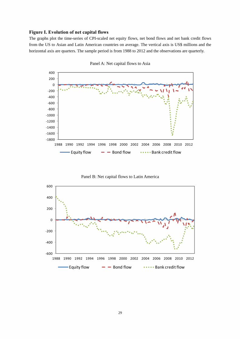
We begin by plotting the time-series of net equity, net bond and net bank credit flows to

Asian and Latin American countries from 1988 to 2012 in Figure I. The vertical axis

represents US$ millions and the horizontal axis is quarters. Several interesting observations 10 These data provide an unusual opportunity for a direct test of the existence of an internal capital market, since data on borrowing and lending within an organization is generally not available to researchers.

10

can be made. First, in the 21st century, bank credit surged and significantly dwarfed the equity

and bond flows. Second, in both Asia and Latin America, the volatility of bond flows and

bank credit flows increased significantly in the 21st century, especially in the run-up to and

during the late 2000s GFC. Third, it is the bank credit flows, instead of portfolio flows, that

suffered the sharpest reversal during the GFC. These patterns in capital flows in the 2000s

seem quite different from the ones in the 1990s, and raise key questions concerning the

temporariness (i.e., hot money) in each category of capital flows in the recent decade.

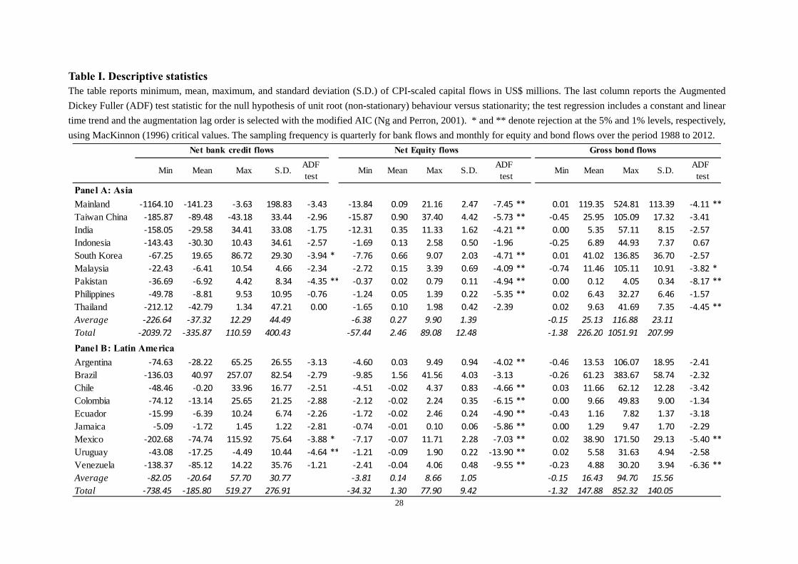
Table I provides summary statistics for net bank credit flows, net equity flows and gross

bond flows from the US to emerging markets over the period 1988-2012.11 The ADF unit root

test results broadly confirm that bank credit and bond flows have a unit root. However, the

evidence for equity flows is less clearcut as the tests suggest non-stationarity over the early

sample period of Sarno and Taylor (1999a) but stationarity over the full sample. Since there is

no economic theory to suggest that equity flows have a drastically different data generating

process from bank and credit flows, following the extant literature we conceptualize all three

flows as realizations from first-difference stationary processes.12 Hence, it makes sense to

gauge the relative importance of their permanent and stationary components.

All three categories of capital flows to Asia surpass in size those to Latin America over

the period under study. For most countries, the average net bank credit flows are negative,

meaning that the US has been on the whole ‘financed’ by EMs in this category of capital.

Average net equity flows are positive for all Asian countries but, in sharp contrast, mostly

negative for Latin American countries (with the exception of Brazil, which shows a relatively

large positive average net equity flow in contrast to all other Latin American countries, and

Argentina to a lesser extent). Thus, over the sample period the US has financed all Asian EMs

11 As mentioned earlier we use a net measure of equity flows and a gross measure of bond flows to abstract from the effect of sterilization policy actions and other types of reserve operations by the monetary authorities (Chuhan et al., 1998; Taylor and Sarno, 1997; Sarno and Taylor, 1999a; Forbes and Warnock, 2012; Sarno et al., 2012). Appendix B provides summary statistics for net bond flows. 12 Our methodology for the analysis of capital flows rests on the assumption that the dynamics of their unobserved persistent component can be approximated by a random walk model. However, as borne out by the mixed results of the unit root tests, other specifications could be plausible alternatives such as those in the autoregressive fractionally integrated moving average class known as ARFIMA models that can generate very persistent (non)stationary data. The random walk process is adopted because it is rather parsimonious (which helps in identification) and to ensure comparability with the prior literature (see e.g., Sarno and Taylor, 1999a).

11

but only two Latin American countries (Brazil by a large amount, and Argentina) via net

equity flows. However, the size of bank credit flows belittles the size of equity flows. Finally,

capital flows to Asia appear more volatile than the flows to Latin America in all categories.

4. State-Space Models

Our analysis of the dynamics of capital flows is based on state-space (or unobserved

components) models. One benefit of representing a dynamic system in state space form is

that unobserved variables can be incorporated and estimated along with the observable

variables. State space models have been widely used in economics to model latent variables

such as (rational) expectations, permanent income and unobserved components such as trends

and cycles. State-space models will allow us to decompose the observed bank, equity and

bond flows into unobserved permanent and temporary components as it is explained next.

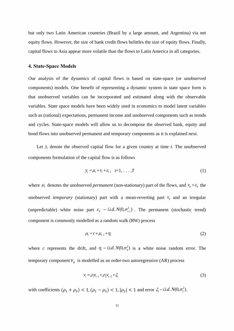
Let ty denote the observed capital flow for a given country at time t. The unobserved

components formulation of the capital flow is as follows

t t t ty v , t=1, . . . ,T (1)

where t denotes the unobserved permanent (non-stationary) part of the flows, and it itv the

unobserved temporary (stationary) part with a mean-reverting part itv and an irregular

(unpredictable) white noise part it ~ 2,. . . (0, ) ii i d N . The permanent (stochastic trend)

component is commonly modelled as a random walk (RW) process

1t t tc (2)

where c represents the drift, and t ~ 2. . . (0, )i i d N is a white noise random error. The

temporary component itv is modelled as an order-two autoregressive (AR) process

1 1 2 2t t t tv v v (3)

with coefficients 1, 1, | | 1 and error t ~ 2. . . (0, )i i d N .

12

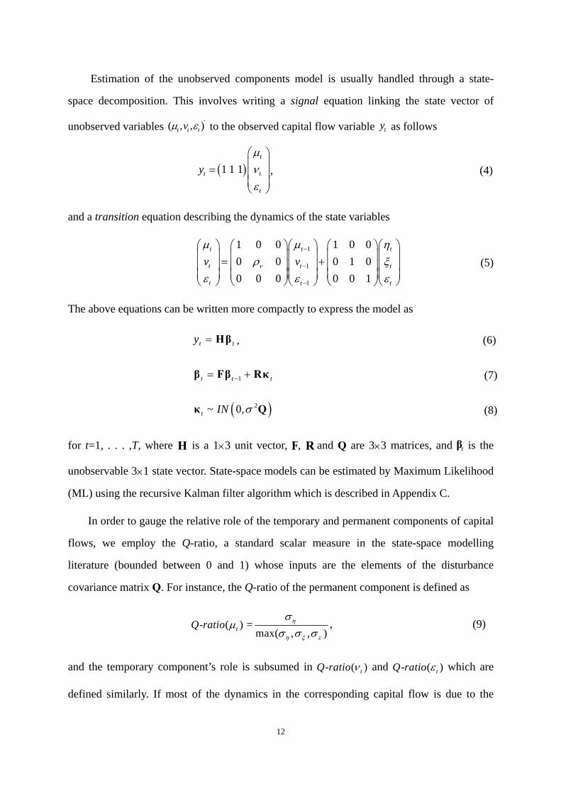
Estimation of the unobserved components model is usually handled through a state-

space decomposition. This involves writing a signal equation linking the state vector of

unobserved variables '( , , )t t tv to the observed capital flow variable ty as follows

1 1 1

t

t t

t

y , (4)

and a transition equation describing the dynamics of the state variables

1

1

1

1 0 0 1 0 0

0 0 0 1 0

0 0 0 0 0 1

t t t

t t t

t t t

v v (5)

The above equations can be written more compactly to express the model as

t ty Hβ , (6)

1t t t β Fβ Rκ (7)

2~ 0,κ Qt IN (8)

for t=1, . . . ,T, where H is a 13 unit vector, F, R and Q are 33 matrices, and tβ is the

unobservable 31 state vector. State-space models can be estimated by Maximum Likelihood

(ML) using the recursive Kalman filter algorithm which is described in Appendix C.

In order to gauge the relative role of the temporary and permanent components of capital

flows, we employ the Q-ratio, a standard scalar measure in the state-space modelling

literature (bounded between 0 and 1) whose inputs are the elements of the disturbance

covariance matrix Q. For instance, the Q-ratio of the permanent component is defined as

- ( ) =max( , , )

tQ ratio , (9)

and the temporary component’s role is subsumed in - ( )tQ ratio and - ( )tQ ratio which are

defined similarly. If most of the dynamics in the corresponding capital flow is due to the

13

permanent component then we expect - ( ) =1tQ ratio which implies that a large part of the

capital flow remains in the country for an indeterminate period of time. Instead, if most of the

variation in the capital flow is explained by the dynamics of the temporary component then

- ( ) =1tQ ratio or - ( ) =1tQ ratio but this finding alone does not allow us to conclude that the

capital flow is dominated by “hot money” because the temporary component could be highly

persistent or slowly mean-reverting. Hence, we need to assess the degree of persistence of

the temporary component of the capital flows for each of the countries concerned.

Many measures of persistence have been employed in the empirical finance literature

and there is no consensus on which one is the most appropriate; see Dias and Marques (2005).

The most popular measures are designed under the so-called univariate approach, namely,

persistence is investigated by looking at the time-series representation of inflation. Following

the latter, in our study a capital flow variable is judged as being dominated by “hot money” if

two conditions are jointly met: i) the Q-ratio of the temporary component is 1, and ii) the

half-life of the temporary component is below one and a half years. As it is standard in the

empirical finance literature, the half-life of a dynamic process is approximated by

1 2 ln( / ) / ln( )H where is the sum of the coefficients of its AR representation.

Appendix D lists the candidate state-space model specifications. We identify the most

appropriate one per country i and category of capital flow using: i) the coefficient of

determination where d is the number of non-stationary elements in

the state vector, and ii) the Akaike information criterion, AIC= log(PEV)+2(m/T), where PEV

is the steady-state prediction error variance, m is the number of unknown parameters to

estimate (the number of the variance parameters, together with damping factors for cycles

and autoregressive coefficients) plus the number of non-stationary components in the state

vector t , and T is the number of observations. For a detailed exposition, see Harvey (1989).

5. Empirical Results

We begin by analyzing the state-space model estimates and diagnostics for bank credit flows

in order to gauge the importance of ‘hot money’. Then we proceed similarly with the equity

22

2

1

ˆ( )1

( )

T

it itt

T dR

y y

14

and bond flows. The analysis is conducted over the 1988-1997, 1997-2012 and full periods.

5.1 Reduced-form unobserved components model

Hot Money in Bank Credit

Has the amount of ‘hot money’ in bank credit flows become more relevant over the recent

decade? To address this question, we discuss the state-space modelling results corresponding

to the first subperiod (1988-1997), extended period (1988-2012) and most recent period

(1998-2012) which are shown in Table II, Panels A, B and C, respectively.

Column 2 of the table notes the selected model specification among all the candidates

considered (listed in Appendix A). The diagnostics shown in the last two columns suggest

that the models provide a good fit: the coefficient of determination (R2) is fairly large, and the

Ljung–Box statistic (p-value) fails to reject the null hypothesis of no residual autocorrelation.

Columns 3-5 report the Q-ratios of the permanent (stochastic trend) component, and the

temporary (AR and/or irregular) components. Column 6 reports the stochastic level in the

final state vector and its root mean square error (RMSE); if the final stochastic level is

significantly different from zero then we can conclude that, even if the Q-ratio of either of the

temporary components is 1, there is a non-negligible permanent component. Column 7 shows

the sum of the AR coefficients (or damping factor 1 2 ) whose proximity to 1

indicates the degree of persistence in the temporary component of the flows; equivalently, the

(unreported) half-life of shocks to the temporary component is a nonlinear transformation of

the damping factor, 1 2 ln( / ) / ln( )H , which is expressed in units of time.

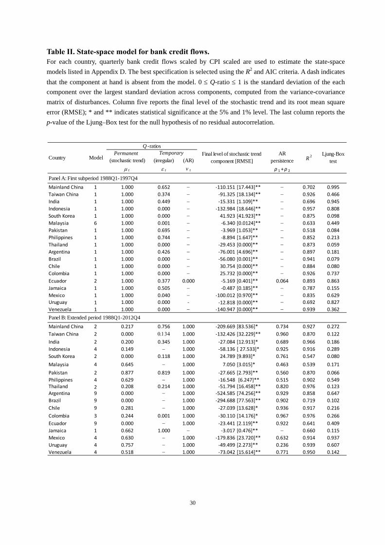
The model estimates for bank credit over the period 1988-1997 suggest for all 18 EMs

the permanent component explains most of the variation in the flows. Taking Mainland China

as an example, the Q-ratio of the permanent component in Table II (Panel A) is equal to 1 and

the Q-ratio of the temporary component is 0.652. Hence, we conclude that bank credit flows

to Asian and Latin American countries from 1988 to 1997 are largely permanent or persistent.

These findings are well aligned with the empirical evidence in Sarno and Taylor (1999a).

15

However, Table II (Panel B) tells a different story. Over the full sample period from

1988 to 2012, the analysis of bank credit flows for both sets of countries suggests that the

largest Q-ratios correspond now instead to the temporary part of the flows, captured by the

vector , . Taking again Mainland China as an example in Table II (Panel B), the Q-ratio

of the stochastic trend component is only 0.217. Therefore, it would seem appropriate to

regard bank credit flows to Mainland China over the full sample period 1988-2012 as largely

influenced by its temporary component which stands in sharp contrast with the evidence from

similar state-space models estimated over the first subsample period 1988-1997. The

contribution of the permanent (temporary) component to the total variation of capital flows is

relatively small (large). The final level of the stochastic trend component is significant

which, together with the Q-ratio, indicates that there is a non-negligible permanent

component in bank credit flows, but it explains a small amount of the total time variation in

bank credit relative to the temporary component. All countries considered, the dynamics of

bank credit flows appear strikingly different over the pre-1990s and 1988-2012 periods.

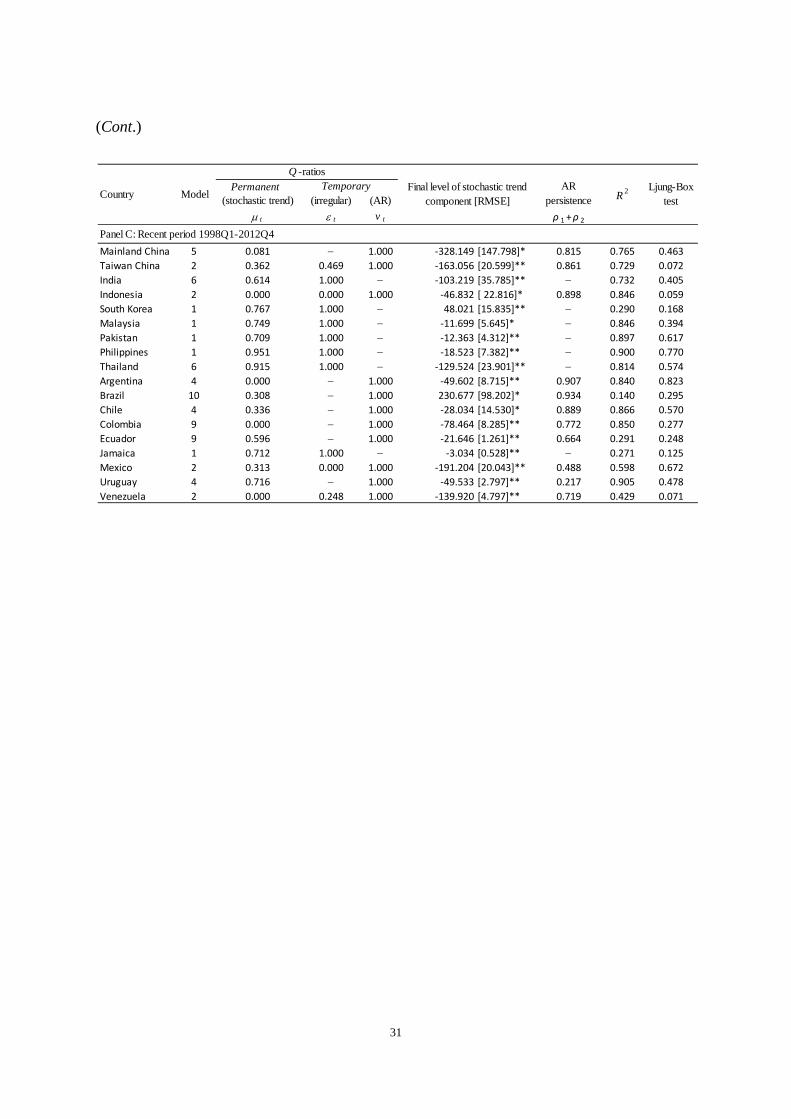
Thus we conjecture that the temporariness of bank credit flows to Asian and Latin

American countries may have increased substantially in the recent decade, coinciding with

the process of banking sector globalisation. To test this conjecture, we re-estimate the models

over the second subsample period 1998-2012. The results are reported in Table II (Panel C).

Bank credit shows now, in contrast to the 1988-1997 period, a large degree of temporariness.

Taking again Mainland China as an example, the two conditions stated in the previous section

are met, namely, the Q-ratio of the AR component is 1 and the corresponding half-life of

shocks at 3.3 quarters is low (below 6 quarters), implying that bank credit to Mainland China

has become dominated by “hot money” over the most recent 15-year period. As clearly

shown in Table II (Panel A), over the first subsample period 1988-1997 none of the countries

meets the two conditions which allows us to conclude that banking flows are dominated by a

permanent component pre-1990s in line with the prior literature. In sharp contrast, as Table II

(Panel C) shows, the same unobserved component models estimated post-1990s reveal that

all countries except two (Argentina and Brazil with half-lives of 7 and 9 quarters, respectively)

meet both conditions. This allows us to conclude that the relative role of “hot money” in bank

16

credit has increased notably in the years leading to and during the GFC.

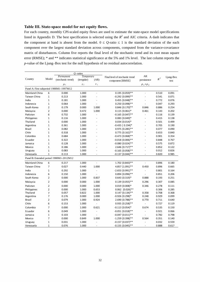
Hot Money in Portfolio Flows

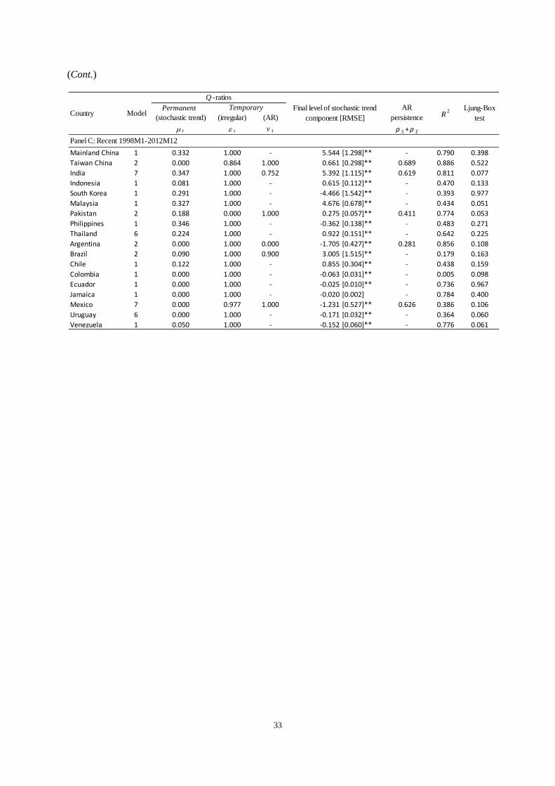
Next we discuss the state-space model estimates and diagnostics for equity and bond flows

which are reported in Tables III and IV, respectively. Again we deploy the models separately

over the three sample periods: 1988-1997, 1988-2012, and 1998-2012. The coefficient of

determination R2 for equity (bond) flows ranges from 0.012 to 0.901 (0.150 to 0.930) in the

1988-1997 analysis and improves to between 0.05 and 0.929 (0.090 and 0.979) in the full

sample analysis. The p-value from the Ljung–Box test uniformly for all 18 EMs and time

periods rules out residual autocorrelation.

In contrast to our findings for bank credit, the largest variance of the disturbances for

portfolio flows is always the temporary component (either irregular or AR component)

consistently across all sample periods. The Q-ratios for the stochastic level components are

low ranging from negligible for equity flows to Mainland China to a maximum of 0.968 for

bond flows to Argentina suggesting that the contribution of the persistent component in

explaining the dynamics of capital flows is low relative to the temporary component. As

borne out by the estimated coefficient of the stochastic level in the final state vector and the

corresponding RMSE (shown in column 4), the permanent component is significant but it

explains a relatively small proportion of the dynamics in the observed flows. Actually, if we

compare the results for bank credit, equity flows and bond flows over the latter sub-sample

from 1998 to 2012, there are large similarities regarding the degree of temporariness. Hence,

all three categories of capital flows have in recent years attained a high degree of reversibility.

Thus, it appears likely that they may have been a channel for the transmission of the GFC.

Summing up, our findings thus far suggest that in the post-1997 era not only bond and

equity flows but also bank credit flows to EMs are characterized by a ‘hot money’ component

that is large relative to the permanent component; this means that all three types of capital

flows are plausible candidates as channels for the transmission of the GFC. Thus, bank credit

surfaces as a new potential channel of crisis transmission given that it appears unlikely as

channel of transmission of previous turmoils such as the 1997 Asian Financial Crisis. The

17

finding of a high reversible component in bank credit flows to EMs is aligned with the recent

literature about rollover risk, the banking sector globalisation and transmission of the GFC.

5.2. Unobserved components model with push/pull factors

A potential criticism of the reduced-form model on which the results thus far are based is that

it lacks economic content. In order to shield our analysis from this criticism, we now

reformulate the state-space models by incorporating one-period lagged macroeconomic

factors as potential exogenous variables both in the permanent and temporary components of

the flows. The aim is to impose some economic ‘structure’ to the state-space models with the

purpose of adding robustness to our key finding that bank credit flows are newly

characterized by a weighty temporary component (hot money) during the post-1997 era. Q-

ratios thus computed from the covariance matrix Q of white noise residuals, account for the

impact of the economic drivers. To our knowledge, no previous study that assesses the

relative importance of the temporary (versus permanent) component of bank credit, equity

and bond flows has deployed ‘structural’ state-space models that control for push/pull factors.

Such models have been mainly used in the context of order flows and high-frequency trading

(Menkveld et al., 2007; Brogaard et al., 2013; Hendershott and Menkveld, 2014).

We employ the following parsimonious state-space model with macro drivers

1 , 11

1 1 2 2 , 1 1 2 2 1 21

,

,

, ( ) 1, ( ) 1, 1

t t t

J

t t j j t tj

J

t t t j j t tj

y v

Z

v v v Z

(10)

where Zj,t denotes the jth macroeconomic factor, and ( , ′ are white noise error terms. The

total number of push/pull factors, J, which cannot be too large due to degrees of freedom

constraints in estimation; to illustrate, the inclusion of say J=5 factors in the state-space

model implies ten additional parameters to estimate.13

13 The above state-space model is an extension of the specification referred to as “Model 5” in Appendix D. It parsimoniously decomposes the flows into a permanent part and a temporary part without irregular components and drifts. After the inclusion of push or push and pull factors as explanatory variables, the irregular component

18

This unobserved components model, equation (10), serves the purpose of addressing the

potential criticism that the original model, equations (1) to (3), is a purely statistical

decomposition of the flows into the latent temporary and permanent parts without any

economic content. Instead, in this reformulation we extract the latent permanent and

temporary components of the capital flows while controlling for various observed factors that

have been shown in previous studies to be potential drivers.

Choosing an appropriate set of pull and push factors {Z1,t, Z2,t,…,ZJ,t} is a non-trivial task

because they ought to be relevant drivers for both the permanent and temporary components.

Earlier studies have considered investor-fear risk, liquidity risk and interest rate risk as push

(or global) factors, and depth of the financial system, real GDP growth, country indebtedness

and capital controls as pull (or domestic) factors (see Forbes and Warnock, 2012; Fratzscher,

2012; Sarno, et al., 2013). However, a parallel literature has suggested other push/pull factors,

that we describe below, as important drivers of hot money. We consider both sets in turn.

Inspired by McKinnon (2013), McKinnon and Liu (2013), McKinnon and Schnabl (2009),

Korinek (2011), and Martin and Morrison (2008), we begin by considering as candidates for

push factors the US interest rate and US equity index; and as pull factors, the EM interest rate,

EM equity index, and the exchange rate defined as units of EM currency per US dollar.

Strictly speaking, however, since the exchange rate has a US side and an EM side, it can be

categorized as either push or a pull factor. Both interest rates and the exchange rate have been

extensively used as drivers in the literature on carry trade, which has been categorised as hot

money.14 We include equity indices for two reasons. First, equity return differences in the US

and EMs could trigger capital flows to globally re-allocate assets, either because of return-

chasing or portfolio-rebalancing motives (Bekaert et al., 2002). Second, the equity market is

commonly seen as a confidence barometer, with a sharp decline often preceding an economic

crisis, which makes hot money in bank credit responsive to the dynamics of the equity market

(Kaminsky and Reinhart 1998, 1999; Kaminsky, 1999; Reinhart and Rogoff, 2009).

and drifts decrease quickly, becoming insignificant. A similar model has been used in a different literature (Menkveld et al., 2007; Brogaard et al., 2013; Hendershott and Menkveld, 2014). 14 The carry trade is a popular currency trading strategy that invests in high-interest currencies by borrowing in low-interest currencies. This strategy is at the core of active currency management and is designed to exploit deviations from uncovered interest parity.

19

Regarding our priors, we expect the US interest rate to impact negatively on capital flows

from the US to EMs, while the interest rate in EMs ought to have a positive impact on capital

flowing from the US to EMs. Since a lower exchange rate means an appreciation of the EM

currency versus the US$ which may arguably attract capital flows into EMs, it is expected

that the exchange rate has a negative impact on capital flows from the US to EMs.

It is harder to form priors about the impact of the US and EMs stock markets on capital

flows because the “return-chasing” and “portfolio-rebalance” hypotheses imply conflicting

predictions (Bekaert et al., 2002). According to the return-chasing hypothesis, the

performance of EMs (the US) stock markets influences positively (negatively) capital flows

from the US to EMs because capital flows chase sizeable stock returns. In sharp contrast,

according to the portfolio-rebalance hypothesis, the EMs (US) stock market performance

affects negatively (positively) capital flows from the US to EMs because investors rebalance

their investment portfolio to maintain their original (planned) asset allocation.

Table V shows the estimation results for the ‘structural’ state-space models of bank

flows using the above factors as lagged (exogenous) drivers over the sample period 1998-

2012. Due to data constraints, we perform the analysis on 8 EMs in our sample. The main

result that the temporary component (hot money) in bank credit flows is responsible for most

of the variation in the flows remains unchallenged. For all 8 EMs, the Q-ratios indicate that

the temporary component weighs more heavily than the permanent component, confirming

the role of hot money during that period. India has the largest Q-ratio for the permanent

component (0.929) across all 8 EMs, followed by Thailand (0.813), Brazil (0.391) and Chile

(0.340), while the Q-ratios of the permanent component for the other four EMs are close to

0.2. The R2 is generally high and the Ljung-Box test suggests no residual autocorrelation.

Looking now at the coefficients of the push and pull factors, our results are consistent with

the previous literature in that international capital flows are highly heterogeneous both over

time and across countries (Milesi-Ferretti and Tile, 2011; Fratzscher, 2012; Warnock and

Forbes, 2012). For example, Fratzscher (2012) finds the effects of economic shocks on

capital flows to be highly heterogeneous across countries, with a large proportion of the

cross-country heterogeneity being ascribed to differences in the quality of domestic

20

institutions, country risk and the strength of domestic macroeconomic fundamentals (pull

factors). But he further shows that push factors were overall the main drivers of capital flows

in the brunt of the GFC, while pull factors have become more dominant in the recent period

2009-2010, in particular, for EMs. Hence, there is evidence in the literature of both time and

cross-country heterogeneity in the role of push/pull factors as drivers of capital flows.

Regarding statistical significance, we find push and pull factors to be equally important;

only marginally, push factors play a more dominant role than pull factors in the permanent

component.15 The heterogeneity of the impact of push and pull factors across countries can be

seen in the close examination of three of the BRIC countries in Sarno et al. (2014), where for

China the importance of the pull factor is close to the world average, for India is much below

the world average and for Brazil for bond flows is much higher than the world average.

The signs of the push/pull factor coefficients are rather mixed in line with the large

heterogeneity (over time and across countries) on the drivers of capital flows documented in

the literature. In our context, it may relate to the fact that the sample includes both crisis and

non-crisis periods. On the one hand, the effects of shocks on capital flows have changed

markedly since the GFC erupted about seven years ago (Fratzscher, 2012). On the other hand,

as it is pointed out in Forbes and Warnock (2012), the same factor may have a different effect

on capital flows when capital flows are in different stages (Surge/Stop/Flight/Retrenchment).

For completeness, we repeat the analysis for push and pull factors used in earlier work.

The push factors are investor-fear risk, liquidity risk and interest rate risk. Investor fear is

proxied by the VXO, a volatility index compiled by the Chicago Board Options Exchange

using S&P 100 option prices, that represents a measure of the market’s expectation of stock

volatility over the next 30 day period.16 Liquidity risk is proxied by year-on-year growth in

US money supply (M2) and the yield on 20-year US government bonds is used for the

interest rate factor. As pull factors, we consider the depth of the financial system (measured

by each country's stock market capitalization divided by GDP), real GDP growth, country

15 We do not count the exchange rate since, as noted above, it can be seen both as a push or a pull factor. 16 The factors we consider are similar to those in Forbes and Warnock (2012). Data on the VIX that tracks the S&P 500 index instead is only available from 2003. As it is shown in Forbes and Warnock (2012), VIX and VXO are very similar. Due also to data constraints, we use growth of money supply instead of TED spread.

21

indebtedness (measured by public debt ratios) and capital controls (measured by Chinn-Ito

indices). The data are obtained from DataStream. The estimation of these ‘structural’ state-

space models is conducted over the full period due to the degrees-of-freedom constraint

imposed by the large number of push/pull factors. The results (unreported for space

constraints but available upon request) affirm that considering this distinct set of push/pull

factors makes no meaningful difference to the findings. The temporary component in bank

credit flows remains responsible for most of the variation in the bank credit flows; which is

likely to reflect (as we saw earlier) the new dynamics in the post-1997 era.

6. Conclusions

Motivated by the dramatic increase in international capital flows in recent years, particularly

in cross-border bank credit flows which reached 60% of global GDP during 2000-2007, this

paper re-examines the role of hot money in bank credit and portfolio flows. We deploy state-

space models à la Kalman filter to evaluate the relative size of the permanent component and

temporary or ‘hot money’ component of the flows from the US to emerging markets (EMs)

over the period 1988 to 2012. A key question we address is whether the degree of

temporariness or potential reversibility of bank flows from the US to EMs has increased in

recent years coinciding with the banking globalisation process.

A key result is that bank credit flows from the US to EMs have undergone a dramatic

change from being predominantly permanent during the 1990s to being mainly temporary (or

reversible) thereafter. This finding is robust to the inclusion of push and pull factors in the

state-space decomposition, an estimation approach not used before in the literature on

international capital flows. Our investigation confirms extant evidence that portfolio flows

(but not bank credit flows) played a major role in the Asian Financial Crisis. The same state-

space models applied to recent data suggest high temporariness of all three types of capital

flows in the new century or equivalently, that all of them have been ‘flooded’ by hot money.

Therefore it appears that bank credit flows are as ‘worrying’ as equity flows for risk managers.

The findings represent tentative evidence that hot money in bank credit and portfolio

flows may have been a potential channel via which the Subprime Crisis in the US evolved

22

into a global financial crisis.17 Thus our analysis indirectly supports the conjecture that bank

lending played a key role in the late 2000s GFC transmission of which Cetorelli and

Goldberg (2011) provide direct evidence from a different methodology. Moreover, the

findings endorse the renewed interest by policymakers in using regulations, sometimes

camouflaged as prudential banking regulations, to manage international capital flows, with

the tacit approval of the IMF (Ostry et al., 2010; McCauley, 2010). An important question

that this paper does not address is what type of bank credit is most responsible for the

observed change from persistence to temporariness in the recent decade. Data limitations at

the time of writing preclude us from pursuing it. We leave this work for further research.

17 It is likely that various other direct channels (such as trade) and/or indirect channel (such as wake-up calls) may also have played an important role in turning the US housing slump into the GFC.

23

Acknowledgements

We are grateful to Roy Batchelor, Keith Cuthbertson, Linda Goldberg, Albert Kyle, Ian Marsh, Anthony Neuberger, Richard Payne, Lucio Sarno and Maik Schmeling for useful suggestions. We also thank participants of the 13th Annual Bank Research Conference in Virginia, US, the 1st Financial Management Conference in Paris, France, 2014, the EMG-ECB 4th Emerging Markets Group Conference at Cass Business School, 2014, and the 14th INFINITI Conference on International Finance in Prato, Italy, 2014.

24

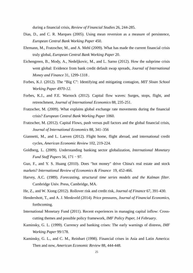
References

Acharya, V. V., Gale, D., and T. Yorulmazer (2011). Rollover risk and market freezes, Journal

of Finance 66, 1177-1209.

Acharya, V.V., and P. Schnabl (2010). Do global banks spread global imbalances? Asset-

backed commercial paper during the financial crisis of 2007–2009, IMF Economic

Review 58, 37-73.

Agosin, M.R., and F. Huaita (2011). Overreaction in capital flows to emerging markets:

Booms and sudden stops, Journal of International Money and Finance 31, 1140-1155.

Aiyar, S. (2012). From financial crisis to great recession: The role of globalized banks,

American Economic Review 102, 225-230.

Bank for International Settlements (2009). Capital flows and emerging market economies,

Bank for International Settlements Papers, January 2009.

Bekaert, G., Harvey, C. R., and R. L. Lumsdaine (2002). The dynamics of emerging market

equity flows, Journal of International Money and Finance 27, 295-350.

Brogaard, J., Hendershott, T., and R. Riordan (2013). High frequency trading and price

discovery, University of Washington Working Paper.

Cetorelli, N., and L. Goldberg (2011). Global banks and international shock transmission:

evidence from the crisis, IMF Economic Review 59, 41–76.

Cetorelli, N., and L. Goldberg (2012a). Banking globalization and monetary transmission,

Journal of Finance 67, 1811–1843.

Cetorelli, N., and L. Goldberg (2012b). Follow the money: Quantifying domestic effects of

foreign bank shocks in the great recession, American Economic Review 102, 213-218.

Chari, V. V., and P. J. Kehoe (2003). Hot money, Journal of Political Economy 111, 1262-

1292.

Chuhan, P., Claessens, S., and N. Mamingi (1998). Equity and bond flows to Latin America

and Asia: The role of global and country factors, Journal of Development Economics 55,

439-463.

Claessens, S., Dooley, M. P., and A. Warner (1995). Portfolio capital flows: Hot or cold?

World Bank Economic Review 9, 153-174.

Cuthbertson, K., Hall, S.G., and M. P. Taylor (1992). Applied econometric techniques.

Harvester Wheatsheaf, Exeter.

De Haas, R., and N. Van Horen (2013). Running for the exit? International bank lending

25

during a financial crisis, Review of Financial Studies 26, 244-285.

Dias, D., and C. R. Marques (2005). Using mean reversion as a measure of persistence,

European Central Bank Working Paper 450.

Ehrmann, M., Fratzscher, M., and A. Mehl (2009). What has made the current financial crisis

truly global, European Central Bank Working Paper 20.

Eichengreen, B., Mody, A., Nedeljkovic, M., and L. Sarno (2012). How the subprime crisis

went global: Evidence from bank credit default swap spreads, Journal of International

Money and Finance 31, 1299-1318 .

Forbes, K.J. (2012). The “Big C”: Identifying and mitigating contagion, MIT Sloan School

Working Paper 4970-12.

Forbes, K.J., and F.E. Warnock (2012). Capital flow waves: Surges, stops, flight, and

retrenchment, Journal of International Economics 88, 235-251.

Fratzscher, M. (2009). What explains global exchange rate movements during the financial

crisis? European Central Bank Working Paper 1060.

Fratzscher, M. (2012). Capital Flows, push versus pull factors and the global financial crisis,

Journal of International Economics 88, 341–356

Giannetti, M., and L. Laeven (2012). Flight home, flight abroad, and international credit

cycles, American Economic Review 102, 219-224.

Goldberg, L. (2009). Understanding banking sector globalization, International Monetary

Fund Staff Papers 56, 171–97.

Guo, F., and Y. S. Huang (2010). Does "hot money" drive China's real estate and stock

markets? International Review of Economics & Finance 19, 452-466.

Harvey, A.C. (1989). Forecasting, structural time series models and the Kalman filter.

Cambridge Univ. Press, Cambridge, MA.

He, Z., and W. Xiong (2012). Rollover risk and credit risk, Journal of Finance 67, 391-430.

Hendershott, T., and A. J. Menkveld (2014). Price pressures, Journal of Financial Economics,

forthcoming.

International Monetary Fund (2011). Recent experiences in managing capital inflow: Cross-

cutting themes and possible policy framework, IMF Policy Paper, 14 February.

Kaminsky, G. L. (1999). Currency and banking crises: The early warnings of distress, IMF

Working Paper 99/178.

Kaminsky, G. L., and C. M., Reinhart (1998). Financial crises in Asia and Latin America:

Then and now, American Economic Review 88, 444-448.

26

Kaminsky, G. L., and C. M., Reinhart (1999). The twin crises: The causes of banking and

balance-of-payments problems, American Economic Review 89, 473-500.

Korinek, A. (2011). Hot money and serial financial crises. IMF Economic Review, 59, 306-

339.

Kamin, S. B., and L. P. DeMarco (2012). How did a domestic housing slump turn into a

global financial crisis? Journal of International Money and Finance 31, 10-41.

Kester, A. Y. (1995). Following the money: US finance in the world economy, National

Academies Press.

Khwaja, A., and A. Mian (2008). Tracing the impact of bank liquidity shocks: Evidence from

an emerging market, American Economic Review 98, 1413–1442.

Levchenko, A. A., and P. Mauro (2007). Do some forms of financial flows help protect

against “sudden stops”? World Bank Economic Review 21, 389-411.

Martin, M. F., and W. M. Morrison (2008). China's hot money problems. Congressional

Research Service Report 22921.

McCauley, R.N. (2010). Managing recent hot money inflows in Asia, in M. Kawai, M.

Lamberte (Eds.), Managing capital flows in Asia: Search for a framework, Edward

Elgar Publishing Ltd. MacKinnon, J. G. (1996). Numerical distribution functions for unit root and cointegration

tests. Journal of Applied Econometrics 11, 601-618.

McKinnon, R. (2013). The unloved dollar standard: From Bretton Woods to the rise of China,

Oxford University Press.

McKinnon, R. and Z. Liu (2013). Zero interest rates in the United States provoke world

monetary instability and constrict the US economy, Review of International Economics

21, 49-56.

McKinnon, R. and G. Schnabl (2009). The case for stabilizing China’s exchange rate: Setting

the stage for fiscal expansion, China and World Economy 17, 1–32.

Menkveld, A. J., Koopman S. J., and A. Lucas (2007). Modeling around-the-clock price

discovery for cross-listed stocks using state space models, Journal of Business and

Economic Statistics, 25, 213–225.

Milesi‐Ferretti, G. M., and C. Tille (2011). The great retrenchment: International capital flows

during the global financial crisis, Economic Policy, 26, 289-346.

Neumann, R.M., Penl R., and A. Tanku (2009). Volatility of capital flows and financial

liberalization: Do specific flows respond differently? International Review of

27

Economics and Finance 18, 488-501.

Ng. S. and P. Perron (2001). Lag length selection and the construction of unit root tests with

good size and power, Econometrica, 69, 1519-1554.

Ostry, J.D., Chamon, M., Qureshi, M.S. Reinhardt, D.B.S. Ghosh, A.R. and K.F. Habermeier

(2010). Capital inflows: The role of controls. IMF Staff Position Note. Washington,

D.C.: International Monetary Fund.

Peek, J. and E. Rosengren (1997). The international transmission of financial shocks: The

case of Japan, The American Economic Review 87, 495-505.

Reinhart, C.M., and K.S. Rogoff (2009). This time is different: Eight centuries of financial

folly, Princeton University Press.

Sarno, L., and M. P. Taylor (1999a). Hot money, accounting labels and the permanence of

capital flows to developing countries: An empirical investigation, Journal of

Development Economics 59, 337-364.

Sarno, L., and M. P. Taylor (1999b). Moral hazard, asset price bubbles, capital flows, and the

East Asian crisis: The first tests, Journal of International Money and Finance 18, 637-

657.

Sarno, L., Tsiakas, I., and B. Ulloa (2013). What drives international portfolio flows? Cass

Business School Working Paper.

Schnabl, P. (2012). Financial globalization and the transmission of bank liquidity shocks:

Evidence from an emerging market, Journal of Finance 67, 897–932.

Tesar, L. L., and I. M. Werner (1994). International equity transactions and US portfolio

choice. In J. Frankel (Ed.) The Internationalization of Equity Markets, University of

Chicago Press.

Tesar, L. L., and I. M. Werner (1995). US equity investment in emerging stock markets,

World Bank Economic Review 9, 109-129.

Tong, H., and S. J.Wei (2011). The composition matters: Capital inflows and liquidity crunch

during a global economic crisis, Review of Financial Studies 24, 2023-2052.

World Bank (2011). World Development Indicators 2011, Washington DC: World Bank.

28

Table I. Descriptive statistics The table reports minimum, mean, maximum, and standard deviation (S.D.) of CPI-scaled capital flows in US$ millions. The last column reports the Augmented

Dickey Fuller (ADF) test statistic for the null hypothesis of unit root (non-stationary) behaviour versus stationarity; the test regression includes a constant and linear

time trend and the augmentation lag order is selected with the modified AIC (Ng and Perron, 2001). * and ** denote rejection at the 5% and 1% levels, respectively,

using MacKinnon (1996) critical values. The sampling frequency is quarterly for bank flows and monthly for equity and bond flows over the period 1988 to 2012.

Min Mean Max S.D.ADF test

Min Mean Max S.D.ADF test

Min Mean Max S.D.ADF test

Mainland ‐1164.10 ‐141.23 ‐3.63 198.83 ‐3.43 ‐13.84 0.09 21.16 2.47 ‐7.45 ** 0.01 119.35 524.81 113.39 ‐4.11 **

Taiwan China ‐185.87 ‐89.48 ‐43.18 33.44 ‐2.96 ‐15.87 0.90 37.40 4.42 ‐5.73 ** ‐0.45 25.95 105.09 17.32 ‐3.41India ‐158.05 ‐29.58 34.41 33.08 ‐1.75 ‐12.31 0.35 11.33 1.62 ‐4.21 ** 0.00 5.35 57.11 8.15 ‐2.57Indonesia ‐143.43 ‐30.30 10.43 34.61 ‐2.57 ‐1.69 0.13 2.58 0.50 ‐1.96 ‐0.25 6.89 44.93 7.37 0.67

South Korea ‐67.25 19.65 86.72 29.30 ‐3.94 * ‐7.76 0.66 9.07 2.03 ‐4.71 ** 0.01 41.02 136.85 36.70 ‐2.57Malaysia ‐22.43 ‐6.41 10.54 4.66 ‐2.34 ‐2.72 0.15 3.39 0.69 ‐4.09 ** ‐0.74 11.46 105.11 10.91 ‐3.82 *

Pakistan ‐36.69 ‐6.92 4.42 8.34 ‐4.35 ** ‐0.37 0.02 0.79 0.11 ‐4.94 ** 0.00 0.12 4.05 0.34 ‐8.17 **

Philippines ‐49.78 ‐8.81 9.53 10.95 ‐0.76 ‐1.24 0.05 1.39 0.22 ‐5.35 ** 0.02 6.43 32.27 6.46 ‐1.57Thailand ‐212.12 ‐42.79 1.34 47.21 0.00 ‐1.65 0.10 1.98 0.42 ‐2.39 0.02 9.63 41.69 7.35 ‐4.45 **

Average ‐226.64 ‐37.32 12.29 44.49 ‐6.38 0.27 9.90 1.39 ‐0.15 25.13 116.88 23.11

Total ‐2039.72 ‐335.87 110.59 400.43 ‐57.44 2.46 89.08 12.48 ‐1.38 226.20 1051.91 207.99

Argentina ‐74.63 ‐28.22 65.25 26.55 ‐3.13 ‐4.60 0.03 9.49 0.94 ‐4.02 ** ‐0.46 13.53 106.07 18.95 ‐2.41Brazil ‐136.03 40.97 257.07 82.54 ‐2.79 ‐9.85 1.56 41.56 4.03 ‐3.13 ‐0.26 61.23 383.67 58.74 ‐2.32Chile ‐48.46 ‐0.20 33.96 16.77 ‐2.51 ‐4.51 ‐0.02 4.37 0.83 ‐4.66 ** 0.03 11.66 62.12 12.28 ‐3.42Colombia ‐74.12 ‐13.14 25.65 21.25 ‐2.88 ‐2.12 ‐0.02 2.24 0.35 ‐6.15 ** 0.00 9.66 49.83 9.00 ‐1.34Ecuador ‐15.99 ‐6.39 10.24 6.74 ‐2.26 ‐1.72 ‐0.02 2.46 0.24 ‐4.90 ** ‐0.43 1.16 7.82 1.37 ‐3.18Jamaica ‐5.09 ‐1.72 1.45 1.22 ‐2.81 ‐0.74 ‐0.01 0.10 0.06 ‐5.86 ** 0.00 1.29 9.47 1.70 ‐2.29Mexico ‐202.68 ‐74.74 115.92 75.64 ‐3.88 * ‐7.17 ‐0.07 11.71 2.28 ‐7.03 ** 0.02 38.90 171.50 29.13 ‐5.40 **

Uruguay ‐43.08 ‐17.25 ‐4.49 10.44 ‐4.64 ** ‐1.21 ‐0.09 1.90 0.22 ‐13.90 ** 0.02 5.58 31.63 4.94 ‐2.58Venezuela ‐138.37 ‐85.12 14.22 35.76 ‐1.21 ‐2.41 ‐0.04 4.06 0.48 ‐9.55 ** ‐0.23 4.88 30.20 3.94 ‐6.36 **

Average ‐82.05 ‐20.64 57.70 30.77 ‐3.81 0.14 8.66 1.05 ‐0.15 16.43 94.70 15.56

Total ‐738.45 ‐185.80 519.27 276.91 ‐34.32 1.30 77.90 9.42 ‐1.32 147.88 852.32 140.05

Net bank credit flows

Panel A: Asia

Panel B: Latin America

Gross bond flowsNet Equity flows

29

Figure I. Evolution of net capital flows The graphs plot the time-series of CPI-scaled net equity flows, net bond flows and net bank credit flows

from the US to Asian and Latin American countries on average. The vertical axis is US$ millions and the

horizontal axis are quarters. The sample period is from 1988 to 2012 and the observations are quarterly.

Panel A: Net capital flows to Asia

Panel B: Net capital flows to Latin America

‐1800

‐1600

‐1400

‐1200

‐1000

‐800

‐600

‐400

‐200

0

200

400

1988 1990 1992 1994 1996 1998 2000 2002 2004 2006 2008 2010 2012

Equity flow Bond flow Bank credit flow

‐600

‐400

‐200

0

200

400

600

1988 1990 1992 1994 1996 1998 2000 2002 2004 2006 2008 2010 2012

Equity flow Bond flow Bank credit flow

30

Table II. State-space model for bank credit flows. For each country, quarterly bank credit flows scaled by CPI scaled are used to estimate the state-space

models listed in Appendix D. The best specification is selected using the R2 and AIC criteria. A dash indicates

that the component at hand is absent from the model. 0 Q-ratio 1 is the standard deviation of the each

component over the largest standard deviation across components, computed from the variance-covariance

matrix of disturbances. Column five reports the final level of the stochastic trend and its root mean square

error (RMSE); * and ** indicates statistical significance at the 5% and 1% level. The last column reports the

p-value of the Ljung–Box test for the null hypothesis of no residual autocorrelation.

Permanent (stochastic trend) (irregular) (AR)

t t v t ρ 1 + ρ 2 

Panel A: First subperiod 1988Q1-1997Q4

Mainland China 1 1.000 0.652 ‐110.151 [17.443]** 0.702 0.995

Taiwan China 1 1.000 0.374 ‐91.325 [18.134]** 0.926 0.466

India 1 1.000 0.449 ‐15.331 [1.109]** 0.696 0.945

Indonesia 1 1.000 0.000 ‐132.984 [18.646]** 0.957 0.808

South Korea 1 1.000 0.000 41.923 [41.923]** 0.875 0.098

Malaysia 6 1.000 0.001 ‐6.340 [0.0124]** 0.633 0.449

Pakistan 1 1.000 0.695 ‐3.969 [1.053]** 0.518 0.084

Philippines 1 1.000 0.744 ‐8.894 [1.647]** 0.852 0.213

Thailand 1 1.000 0.000 ‐29.453 [0.000]** 0.873 0.059

Argentina 1 1.000 0.426 ‐76.001 [4.696]** 0.897 0.181

Brazil 1 1.000 0.000 ‐56.080 [0.001]** 0.941 0.079

Chile 1 1.000 0.000 30.754 [0.000]** 0.884 0.080

Colombia 1 1.000 0.000 25.732 [0.000]** 0.926 0.737

Ecuador 2 1.000 0.377 0.000 ‐5.169 [0.401]** 0.064 0.893 0.863

Jamaica 1 1.000 0.505 ‐0.487 [0.185]** 0.787 0.155

Mexico 1 1.000 0.040 ‐100.012 [0.970]** 0.835 0.629

Uruguay 1 1.000 0.000 ‐ ‐12.818 [0.000]** 0.692 0.827

Venezuela 1 1.000 0.000 ‐140.947 [0.000]** 0.939 0.362

Panel B: Extended period 1988Q1-2012Q4

Mainland China 2 0.217 0.756 1.000 ‐209.669 [83.536]* 0.734 0.927 0.272

Taiwan China 2 0.000 1.000 ‐132.426 [32.229]** 0.960 0.870 0.122

India 2 0.200 0.345 1.000 ‐27.084 [12.913]* 0.689 0.966 0.186

Indonesia 4 0.149 1.000 ‐58.136 [ 27.533]* 0.925 0.916 0.289

South Korea 2 0.000 0.118 1.000 24.789 [9.893]* 0.761 0.547 0.080

Malaysia 4 0.645 1.000 7.050 [3.015]* 0.463 0.539 0.171

Pakistan 2 0.877 0.819 1.000 ‐27.665 [2.793]** 0.560 0.870 0.066

Philippines 4 0.629 1.000 ‐16.548 [6.247]** 0.515 0.902 0.549Thailand 2 0.208 0.214 1.000 ‐51.794 [16.458]** 0.820 0.976 0.123Argentina 9 0.000 1.000 ‐524.585 [74.256]** 0.929 0.858 0.647

Brazil 9 0.000 1.000 ‐294.688 [77.563]** 0.902 0.719 0.102

Chile 9 0.281 1.000 ‐27.039 [13.628]* 0.936 0.917 0.216

Colombia 3 0.244 0.001 1.000 ‐30.110 [14.176]* 0.967 0.976 0.266

Ecuador 9 0.000 1.000 ‐23.441 [2.119]** 0.922 0.641 0.409

Jamaica 1 0.662 1.000 ‐3.017 [0.476]** 0.660 0.115

Mexico 4 0.630 1.000 ‐179.836 [23.720]** 0.632 0.914 0.937

Uruguay 4 0.757 1.000 ‐49.499 [2.273]** 0.236 0.939 0.607

Venezuela 4 0.518 1.000 ‐73.042 [15.614]** 0.771 0.950 0.142

Q -ratios Temporary Ljung-Box

testR 2AR persistence

Final level of stochastic trend component [RMSE]

ModelCountry

31

(Cont.)

Permanent (stochastic trend) (irregular) (AR)

t t v t ρ 1 + ρ 2 

Panel C: Recent period 1998Q1-2012Q4

Mainland China 5 0.081 1.000 ‐328.149 [147.798]* 0.815 0.765 0.463

Taiwan China 2 0.362 0.469 1.000 ‐163.056 [20.599]** 0.861 0.729 0.072

India 6 0.614 1.000 ‐103.219 [35.785]** 0.732 0.405

Indonesia 2 0.000 0.000 1.000 ‐46.832 [ 22.816]* 0.898 0.846 0.059

South Korea 1 0.767 1.000 48.021 [15.835]** 0.290 0.168

Malaysia 1 0.749 1.000 ‐11.699 [5.645]* 0.846 0.394

Pakistan 1 0.709 1.000 ‐12.363 [4.312]** 0.897 0.617

Philippines 1 0.951 1.000 ‐18.523 [7.382]** 0.900 0.770

Thailand 6 0.915 1.000 ‐129.524 [23.901]** 0.814 0.574

Argentina 4 0.000 1.000 ‐49.602 [8.715]** 0.907 0.840 0.823

Brazil 10 0.308 1.000 230.677 [98.202]* 0.934 0.140 0.295

Chile 4 0.336 1.000 ‐28.034 [14.530]* 0.889 0.866 0.570

Colombia 9 0.000 1.000 ‐78.464 [8.285]** 0.772 0.850 0.277

Ecuador 9 0.596 1.000 ‐21.646 [1.261]** 0.664 0.291 0.248

Jamaica 1 0.712 1.000 ‐3.034 [0.528]** 0.271 0.125

Mexico 2 0.313 0.000 1.000 ‐191.204 [20.043]** 0.488 0.598 0.672

Uruguay 4 0.716 1.000 ‐49.533 [2.797]** 0.217 0.905 0.478

Venezuela 2 0.000 0.248 1.000 ‐139.920 [4.797]** 0.719 0.429 0.071

AR persistence R 2 Ljung-Box

test

Q -ratios Temporary

Country ModelFinal level of stochastic trend

component [RMSE]

32

Table III. State-space model for net equity flows. For each country, monthly CPI-scaled equity flows are used to estimate the state-space model specifications

listed in Appendix D. The best specification is selected using the R2 and AIC criteria. A dash indicates that

the component at hand is absent from the model. 0 Q-ratio 1 is the standard deviation of the each

component over the largest standard deviation across components, computed from the variance-covariance

matrix of disturbances. Column five reports the final level of the stochastic trend and its root mean square

error (RMSE); * and ** indicates statistical significance at the 5% and 1% level. The last column reports the

p-value of the Ljung–Box test for the null hypothesis of no residual autocorrelation.

Permanent (stochastic trend) (irregular) (AR)

t t v t ρ 1 + ρ 2 

Panel A: First subperiod 1988M1-1997M12

Mainland China 6 0.000 1.000 ‐ 0.195 [0.059]** ‐ 0.510 0.091

Taiwan China 1 0.213 1.000 ‐ ‐0.292 [0.099]** ‐ 0.541 0.071

India 1 0.181 1.000 ‐ 0.455 [0.048]** ‐ 0.772 0.076

Indonesia 1 0.064 1.000 ‐ 0.250 [0.098]** ‐ 0.047 0.293

South Korea 2 0.179 0.000 1.000 0.846 [0.170]** 0.846 0.886 0.254

Malaysia 2 0.000 0.472 1.000 0.115 [0.061]* 0.461 0.143 0.202

Pakistan 6 0.732 1.000 ‐ ‐0.165 [0.047]** ‐ 0.116 0.139

Philippines 1 0.116 1.000 ‐ 0.083 [0.049]* ‐ 0.415 0.138

Thailand 1 0.000 1.000 ‐ 0.034 [0.014]* ‐ 0.501 0.499

Argentina 1 0.361 1.000 ‐ ‐0.435 [ 0.194]* ‐ 0.705 0.190

Brazil 1 0.082 1.000 ‐ 0.975 [0.285]** ‐ 0.077 0.090

Chile 1 0.318 1.000 ‐ 0.775 [0.162]** ‐ 0.653 0.840

Colombia 1 0.684 1.000 ‐ ‐0.473 [0.068]** ‐ 0.901 0.354

Ecuador 1 0.322 1.000 ‐ ‐0.018 [0.006]** ‐ 0.848 0.767

Jamaica 1 0.128 1.000 ‐ ‐0.080 [0.024]** ‐ 0.575 0.872

Mexico 1 0.186 1.000 ‐ 2.646 [0.717]** ‐ 0.852 0.122Uruguay 1 0.083 1.000 ‐ ‐0.165 [0.058]** ‐ 0.012 0.826

Venezuela 1 0.113 1.000 ‐ ‐0.137 [0.044]** ‐ 0.820 0.985

Panel B: Extended period 1988M1-2012M12

Mainland China 6 0.217 1.000 ‐ 1.702 [0.843]** ‐ 0.896 0.180

Taiwan China 7 0.027 0.440 1.000 4.857 [1.091]** 0.450 0.896 0.665

India 1 0.292 1.000 ‐ ‐2.653 [0.991]** ‐ 0.801 0.164

Indonesia 6 0.150 1.000 ‐ 0.894 [0.096]** ‐ 0.851 0.206

South Korea 2 0.000 1.000 0.837 0.643 [0.319]* 0.888 0.193 0.251

Malaysia 2 0.000 0.000 1.000 0.139 [0.055]** 0.296 0.307 0.085

Pakistan 2 0.000 0.000 1.000 0.019 [0.008]* 0.346 0.278 0.111

Philippines 2 0.000 1.000 0.653 0.062 [0.026]** ‐ 0.306 0.285Thailand 7 0.057 0.822 1.000 0.147 [0.134]** 0.358 0.708 0.368Argentina 7 0.176 0.000 1.000 ‐0.926 [0.298]* 0.248 0.929 0.099

Brazil 2 0.079 1.000 0.924 2.690 [0.788]** 0.770 0.711 0.640

Chile 6 0.153 1.000 ‐ 0.935 [0.258]** ‐ 0.727 0.119

Colombia 7 0.000 1.000 0.621 ‐0.113 [0.054]* 0.674 0.535 0.150

Ecuador 6 0.049 1.000 ‐ ‐0.051 [0.018]** ‐ 0.921 0.066

Jamaica 1 0.103 1.000 ‐ ‐0.047 [0.011]** ‐ 0.782 0.798

Mexico 7 0.000 0.849 1.000 ‐1.259 [0.398]** 0.564 0.351 0.140

Uruguay 1 0.031 1.000 ‐ ‐0.157 [0.037]** ‐ 0.032 0.559

Venezuela 1 0.076 1.000 ‐ ‐0.155 [0.045]** ‐ 0.888 0.617

Q -ratios Temporary

Country ModelFinal level of stochastic trend

component [RMSE]

AR persistence R 2 Ljung-Box

test

33

(Cont.)

Permanent (stochastic trend) (irregular) (AR)

t t v t ρ 1 + ρ 2 

Panel C: Recent 1998M1-2012M12

Mainland China 1 0.332 1.000 ‐ 5.544 [1.298]** ‐ 0.790 0.398

Taiwan China 2 0.000 0.864 1.000 0.661 [0.298]** 0.689 0.886 0.522

India 7 0.347 1.000 0.752 5.392 [1.115]** 0.619 0.811 0.077

Indonesia 1 0.081 1.000 ‐ 0.615 [0.112]** ‐ 0.470 0.133

South Korea 1 0.291 1.000 ‐ ‐4.466 [1.542]** ‐ 0.393 0.977

Malaysia 1 0.327 1.000 ‐ 4.676 [0.678]** ‐ 0.434 0.051

Pakistan 2 0.188 0.000 1.000 0.275 [0.057]** 0.411 0.774 0.053

Philippines 1 0.346 1.000 ‐ ‐0.362 [0.138]** ‐ 0.483 0.271

Thailand 6 0.224 1.000 ‐ 0.922 [0.151]** ‐ 0.642 0.225

Argentina 2 0.000 1.000 0.000 ‐1.705 [0.427]** 0.281 0.856 0.108

Brazil 2 0.090 1.000 0.900 3.005 [1.515]** ‐ 0.179 0.163

Chile 1 0.122 1.000 ‐ 0.855 [0.304]** ‐ 0.438 0.159

Colombia 1 0.000 1.000 ‐ ‐0.063 [0.031]** ‐ 0.005 0.098

Ecuador 1 0.000 1.000 ‐ ‐0.025 [0.010]** ‐ 0.736 0.967

Jamaica 1 0.000 1.000 ‐ ‐0.020 [0.002] ‐ 0.784 0.400

Mexico 7 0.000 0.977 1.000 ‐1.231 [0.527]** 0.626 0.386 0.106

Uruguay 6 0.000 1.000 ‐ ‐0.171 [0.032]** ‐ 0.364 0.060

Venezuela 1 0.050 1.000 ‐ ‐0.152 [0.060]** ‐ 0.776 0.061

Q -ratios Temporary

Country ModelFinal level of stochastic trend

component [RMSE]AR

persistence R 2 Ljung-Box test

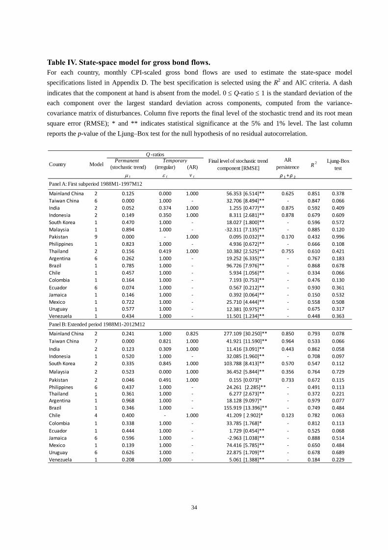
34

Table IV. State-space model for gross bond flows. For each country, monthly CPI-scaled gross bond flows are used to estimate the state-space model

specifications listed in Appendix D. The best specification is selected using the R2 and AIC criteria. A dash

indicates that the component at hand is absent from the model. 0 Q-ratio 1 is the standard deviation of the

each component over the largest standard deviation across components, computed from the variance-

covariance matrix of disturbances. Column five reports the final level of the stochastic trend and its root mean

square error (RMSE); * and ** indicates statistical significance at the 5% and 1% level. The last column

reports the p-value of the Ljung–Box test for the null hypothesis of no residual autocorrelation.

Permanent (stochastic trend) (irregular) (AR)

t t v t ρ 1 + ρ 2 

Panel A: First subperiod 1988M1-1997M12

Mainland China 2 0.125 0.000 1.000 56.353 [6.514]** 0.625 0.851 0.378

Taiwan China 6 0.000 1.000 ‐ 32.706 [8.494]** ‐ 0.847 0.066

India 2 0.052 0.374 1.000 1.255 [0.477]** 0.875 0.592 0.409

Indonesia 2 0.149 0.350 1.000 8.311 [2.681]** 0.878 0.679 0.609

South Korea 1 0.470 1.000 ‐ 18.027 [1.800]** ‐ 0.596 0.572

Malaysia 1 0.894 1.000 ‐ ‐32.311 [7.135]** ‐ 0.885 0.120

Pakistan 9 0.000 ‐ 1.000 0.095 [0.032]** 0.170 0.432 0.996

Philippines 1 0.823 1.000 ‐ 4.936 [0.672]** ‐ 0.666 0.108

Thailand 2 0.156 0.419 1.000 10.382 [2.525]** 0.755 0.610 0.421

Argentina 6 0.262 1.000 ‐ 19.252 [6.335]** ‐ 0.767 0.183

Brazil 1 0.785 1.000 ‐ 96.726 [7.976]** ‐ 0.868 0.678

Chile 1 0.457 1.000 ‐ 5.934 [1.056]** ‐ 0.334 0.066

Colombia 1 0.164 1.000 ‐ 7.193 [0.753]** ‐ 0.476 0.130

Ecuador 6 0.074 1.000 ‐ 0.567 [0.212]** ‐ 0.930 0.361

Jamaica 1 0.146 1.000 ‐ 0.392 [0.064]** ‐ 0.150 0.532

Mexico 1 0.722 1.000 ‐ 25.710 [4.444]** ‐ 0.558 0.508Uruguay 1 0.577 1.000 ‐ 12.381 [0.975]** ‐ 0.675 0.317

Venezuela 1 0.434 1.000 ‐ 11.501 [1.234]** ‐ 0.448 0.363

Panel B: Extended period 1988M1-2012M12

Mainland China 2 0.241 1.000 0.825 277.109 [30.250]** 0.850 0.793 0.078

Taiwan China 7 0.000 0.821 1.000 41.921 [11.590]** 0.964 0.533 0.066

India 2 0.123 0.309 1.000 11.416 [3.091]** 0.443 0.862 0.058

Indonesia 1 0.520 1.000 ‐ 32.085 [1.960]** ‐ 0.708 0.097

South Korea 2 0.335 0.845 1.000 103.788 [8.413]** 0.570 0.547 0.112

Malaysia 2 0.523 0.000 1.000 36.452 [5.844]** 0.356 0.764 0.729

Pakistan 2 0.046 0.491 1.000 0.155 [0.073]* 0.733 0.672 0.115

Philippines 6 0.437 1.000 ‐ 24.261 [2.285]** ‐ 0.491 0.113Thailand 1 0.361 1.000 ‐ 6.277 [2.673]** ‐ 0.372 0.221Argentina 1 0.968 1.000 ‐ 18.128 [9.097]* ‐ 0.979 0.077

Brazil 1 0.346 1.000 ‐ 155.919 [13.396]** ‐ 0.749 0.484

Chile 4 0.400 ‐ 1.000 41.209 [ 2.902]* 0.123 0.782 0.063

Colombia 1 0.338 1.000 ‐ 33.785 [1.768]* ‐ 0.812 0.113

Ecuador 1 0.444 1.000 ‐ 1.729 [0.454]** ‐ 0.525 0.068

Jamaica 6 0.596 1.000 ‐ ‐2.963 [1.038]** ‐ 0.888 0.514

Mexico 1 0.139 1.000 ‐ 74.416 [5.785]** ‐ 0.650 0.484

Uruguay 6 0.626 1.000 ‐ 22.875 [1.709]** ‐ 0.678 0.689

Venezuela 1 0.208 1.000 ‐ 5.061 [1.388]** ‐ 0.184 0.229

Q -ratios Temporary

Country ModelFinal level of stochastic trend

component [RMSE]

AR persistence R 2 Ljung-Box

test

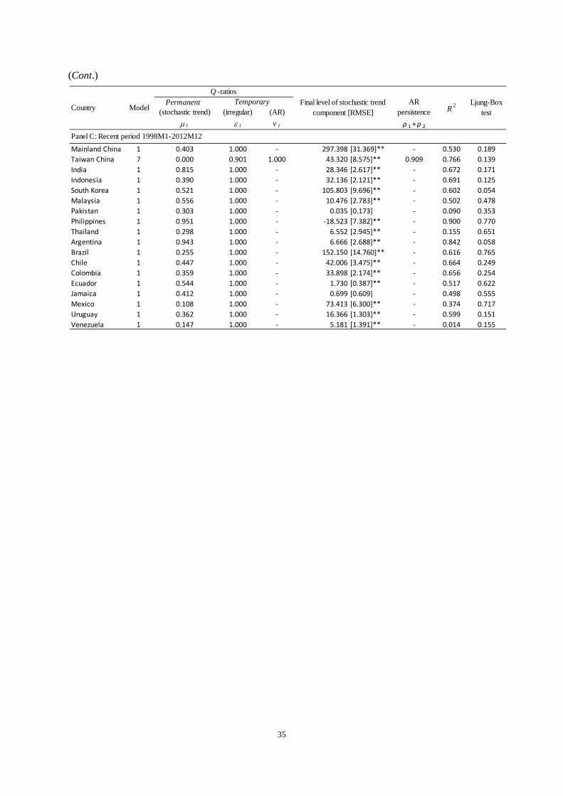
35

(Cont.)

Permanent (stochastic trend) (irregular) (AR)

t t v t ρ 1 + ρ 2 

Panel C: Recent period 1998M1-2012M12

Mainland China 1 0.403 1.000 ‐ 297.398 [31.369]** ‐ 0.530 0.189

Taiwan China 7 0.000 0.901 1.000 43.320 [8.575]** 0.909 0.766 0.139

India 1 0.815 1.000 ‐ 28.346 [2.617]** ‐ 0.672 0.171

Indonesia 1 0.390 1.000 ‐ 32.136 [2.121]** ‐ 0.691 0.125

South Korea 1 0.521 1.000 ‐ 105.803 [9.696]** ‐ 0.602 0.054

Malaysia 1 0.556 1.000 ‐ 10.476 [2.783]** ‐ 0.502 0.478

Pakistan 1 0.303 1.000 ‐ 0.035 [0.173] ‐ 0.090 0.353

Philippines 1 0.951 1.000 ‐ ‐18.523 [7.382]** ‐ 0.900 0.770

Thailand 1 0.298 1.000 ‐ 6.552 [2.945]** ‐ 0.155 0.651

Argentina 1 0.943 1.000 ‐ 6.666 [2.688]** ‐ 0.842 0.058

Brazil 1 0.255 1.000 ‐ 152.150 [14.760]** ‐ 0.616 0.765

Chile 1 0.447 1.000 ‐ 42.006 [3.475]** ‐ 0.664 0.249

Colombia 1 0.359 1.000 ‐ 33.898 [2.174]** ‐ 0.656 0.254

Ecuador 1 0.544 1.000 ‐ 1.730 [0.387]** ‐ 0.517 0.622

Jamaica 1 0.412 1.000 ‐ 0.699 [0.609] ‐ 0.498 0.555

Mexico 1 0.108 1.000 ‐ 73.413 [6.300]** ‐ 0.374 0.717

Uruguay 1 0.362 1.000 ‐ 16.366 [1.303]** ‐ 0.599 0.151

Venezuela 1 0.147 1.000 ‐ 5.181 [1.391]** ‐ 0.014 0.155

Final level of stochastic trend component [RMSE]

AR persistence R 2 Ljung-Box

test

Q -ratios Temporary

Country Model

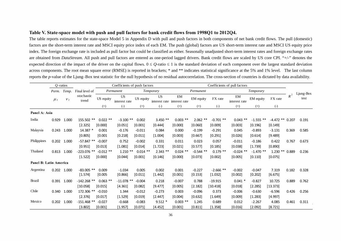
36

Table V. State-space model with push and pull factors for bank credit flows from 1998Q1 to 2012Q4. The table reports estimates for the state-space Model 5 in Appendix D with pull and push factors in both components of net bank credit flows. The pull (domestic)

factors are the short-term interest rate and MSCI equity price index of each EM. The push (global) factors are US short-term interest rate and MSCI US equity price

index. The foreign exchange rate is included as pull factor but could be classified as either. Seasonally unadjusted short-term interest rates and foreign exchange rates

are obtained from DataStream. All push and pull factors are entered as one-period lagged drivers. Bank credit flows are scaled by US core CPI. “+/-” denotes the

expected direction of the impact of the driver on the capital flows. 0 Q-ratio 1 is the standard deviation of each component over the largest standard deviation

across components. The root mean square error (RMSE) is reported in brackets; * and ** indicates statistical significance at the 5% and 1% level. The last column

reports the p-value of the Ljung–Box test statistic for the null hypothesis of no residual autocorrelation. The cross-section of countries is dictated by data availability.

Perm. Temp.

t t

Panel A: Asia

India 0.929 1.000 155.502 ** 0.022 ** ‐3.100 0.002 3.450 0.003 ** 2.062 ** ‐0.701 0.043 ** ‐1.555 ** ‐4.472 0.207 0.191

[2.325] [0.000] [0.051] [0.001] [0.444] [0.000] [0.060] [0.009] [0.003] [0.196] [0.149]

Malaysia 0.243 1.000 14.387 * 0.001 ‐0.176 ‐0.011 0.084 0.000 ‐0.199 ‐0.291 0.045 ‐0.893 ‐3.131 0.369 0.585

[0.805] [0.001 [0.218] [0.011] [1.004] [0.003] [0.667] [0.291] [0.026] [0.614] [9.489]

Philippines 0.202 1.000 ‐57.847 ** ‐0.007 0.752 ‐0.002 0.331 0.011 0.023 0.057 ‐0.011 ‐0.186 0.422 0.767 0.673

[0.951] [0.013] [1.081] [0.014] [1.723] [0.021] [0.577] [0.185] [0.038] [1.739] [0.890]Thailand 0.813 1.000 ‐223.076 ** ‐0.012 ** 1.210 0.014 ** 2.343 0.024 ** ‐0.544 ** 0.179 ‐0.024 ** ‐1.470 ** 1.230 0.889 0.236

[1.522] [0.000] [0.044] [0.001] [0.146] [0.000] [0.073] [0.002] [0.005] [0.110] [0.075]

Argentina 0.202 1.000 ‐83.005 ** 0.009 ‐1.034 0.005 0.002 0.001 ‐0.227 ‐2.666 ‐0.002 ‐0.047 7.319 0.182 0.328[1.574] [0.005 [0.866] [0.011] [1.442] [0.001] [0.153] [1.032] [0.002] [0.202] [6.675]

Brazil 0.391 1.000 ‐142.268 ** 0.063 ** ‐11.078 ‐0.004 0.218 ‐0.007 0.788 ‐19.915 0.041 * ‐0.827 10.725 0.889 0.762

[10.058] [0.015] [4.361] [0.082] [9.477] [0.005] [2.182] [10.418] [0.018] [2.285] [13.373]Chile 0.340 1.000 172.306 ** ‐0.010 1.344 ‐0.012 ‐0.273 0.003 ‐0.096 0.373 ‐0.006 ‐0.630 ‐6.596 0.426 0.256

[2.376] [0.017] [1.529] [0.019] [2.447] [0.004] [0.632] [1.649] [0.009] [1.283] [4.997]Mexico 0.202 1.000 ‐151.468 ** ‐0.027 ‐0.668 ‐0.083 9.512 0.003 ** 1.245 0.689 0.012 ‐2.267 4.085 0.461 0.311

[3.802] [0.001] [1.957] [0.071] [4.452] [0.001] [0.811] [1.358] [0.016] [2.092] [8.721]

Q -ratios Coefficients of push factors

R2 Ljung-Box

test

Temporary Permanent Temporary

Coefficients of pull factors

EM interest rate

EM equity FX rate

(+) (+) (-)

** ** ** **

** ** **

*

**

**

Panel B: Latin America

Final level of stochastic

trend

(+) (-) (+) (-)

**

EM equity FX rate

(+) (+) (-)

US interest rate

US interest rate

US equity US equity EM

interest rate

Permanent

37

Appendix A. International capital form S and international capital form B.

This appendix summarizes key information from the US Department of Treasury’s “Instructions for

Preparation of Monthly Form S” and “Instructions for Preparation of Monthly Form B” available, at

http://www.treas.gov/tic/forms-s.shtml and http://www.treas.gov/tic/forms-b.shtml, respectively.

All banks, brokers, dealers (and other financial institutions) and individuals are by law required to

report the value of any long-term security transactions involving a foreign resident. American Depositary

Receipts (ADR) transactions are included. Securities transactions are reported on a transactions basis.

Securities transactions are recorded by the nationality of the person with whom the transaction is carried, not

by the country that originally issued the security. A foreigner is any individual, branch, partnership,

association, corporation or other organization located outside the United States. Additionally, securities are

recorded according to the residency of the issuer and not their currency denomination.

The data collection system is specifically designed to capture US cross- border financial transactions for

balance-of-payment purposes. That is, it is designed to capture only financial transactions that involve both a

US resident and a foreign resident. Note that a US resident includes any individual, corporation, or

organization located in the United States including branches, subsidiaries, and affiliates of foreign entities

located in the United States. In addition, any corporation incorporated in the United States is considered a

US resident even if it has no physical presence. Thus, a US branch of a Japanese bank is considered a US

resident, and a London branch of a US bank is considered a foreign resident.

The cross-border definition means that the data on foreign purchases of US securities include only those

transactions that involve both a US seller and a foreign purchaser. Thus, these data exclude any US-to-US

transactions, including, for example, transactions where the seller is a US securities broker and the purchaser

is a US-based branch of a Japanese securities firm. They also exclude foreign-to-foreign transactions in

securities, for example if a Japanese-resident securities broker purchases US Treasuries from a London-based

securities broker. Because many US securities, including US Treasury securities, trade in foreign financial

markets, the data will not capture all foreign transactions in US securities.

These forms are the basis for the collection of data on purchases and sales of long-term securities, bank

liabilities and bank claims by foreigners. The Treasury uses these data to provide timely and reliable

information on international capital movements. This information is needed for preparation of the US capital

accounts of the US balance-of-payment and the international investment position of the United States. These

reports cover transaction by all banks, brokers, dealers, other financial institutions and individuals who carry

transactions directly with foreigners.

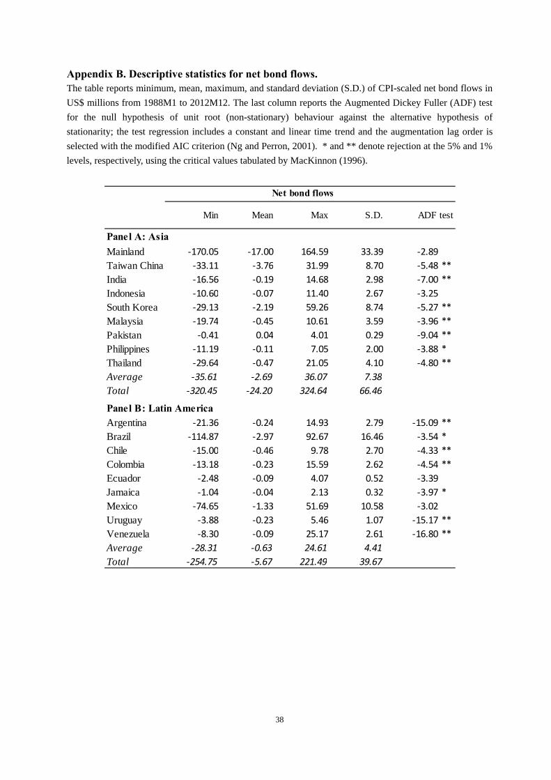
38

Appendix B. Descriptive statistics for net bond flows. The table reports minimum, mean, maximum, and standard deviation (S.D.) of CPI-scaled net bond flows in

US$ millions from 1988M1 to 2012M12. The last column reports the Augmented Dickey Fuller (ADF) test

for the null hypothesis of unit root (non-stationary) behaviour against the alternative hypothesis of

stationarity; the test regression includes a constant and linear time trend and the augmentation lag order is

selected with the modified AIC criterion (Ng and Perron, 2001). * and ** denote rejection at the 5% and 1%

levels, respectively, using the critical values tabulated by MacKinnon (1996).

Min Mean Max S.D.

Mainland ‐170.05 ‐17.00 164.59 33.39 ‐2.89Taiwan China ‐33.11 ‐3.76 31.99 8.70 ‐5.48 **

India ‐16.56 ‐0.19 14.68 2.98 ‐7.00 **

Indonesia ‐10.60 ‐0.07 11.40 2.67 ‐3.25South Korea ‐29.13 ‐2.19 59.26 8.74 ‐5.27 **

Malaysia ‐19.74 ‐0.45 10.61 3.59 ‐3.96 **

Pakistan ‐0.41 0.04 4.01 0.29 ‐9.04 **

Philippines ‐11.19 ‐0.11 7.05 2.00 ‐3.88 *

Thailand ‐29.64 ‐0.47 21.05 4.10 ‐4.80 **

Average ‐35.61 ‐2.69 36.07 7.38

Total ‐320.45 ‐24.20 324.64 66.46

Argentina ‐21.36 ‐0.24 14.93 2.79 ‐15.09 **

Brazil ‐114.87 ‐2.97 92.67 16.46 ‐3.54 *

Chile ‐15.00 ‐0.46 9.78 2.70 ‐4.33 **

Colombia ‐13.18 ‐0.23 15.59 2.62 ‐4.54 **

Ecuador ‐2.48 ‐0.09 4.07 0.52 ‐3.39Jamaica ‐1.04 ‐0.04 2.13 0.32 ‐3.97 *

Mexico ‐74.65 ‐1.33 51.69 10.58 ‐3.02Uruguay ‐3.88 ‐0.23 5.46 1.07 ‐15.17 **

Venezuela ‐8.30 ‐0.09 25.17 2.61 ‐16.80 **

Average ‐28.31 ‐0.63 24.61 4.41

Total ‐254.75 ‐5.67 221.49 39.67

Net bond flows

Panel A: Asia

Panel B: Latin America

ADF test

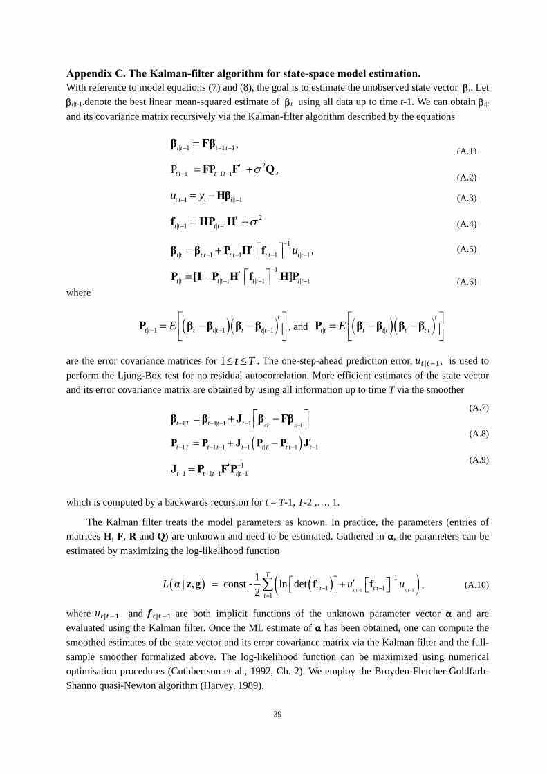
39

Appendix C. The Kalman-filter algorithm for state-space model estimation. With reference to model equations (7) and (8), the goal is to estimate the unobserved state vector t. Let

t|t-1.denote the best linear mean-squared estimate of t using all data up to time t-1. We can obtain t|t

and its covariance matrix recursively via the Kalman-filter algorithm described by the equations

| 1 1| 1 t t t tβ Fβ ,

(A.1)

| 1 1|2

1P P t t t tF F Q ,

(A.2)

t || 11 t tt tyu Hβ

(A.3)

2| 1 | 1t t t t f HP H

(A.4)

1

| | 1 | 1 | 1 | 1t t t t t t t t t tu

β β P H f ,

(A.5)

1

| | 1 | 1 | 1[ ]t t t t t t t t

P I P H f H P

(A.6)where

| 1 | 1 | 1t t t t t t t tE

P β β β β , and | | |t t t t t t t tE

P β β β β

are the error covariance matrices for 1 t T . The one-step-ahead prediction error, | , is used to

perform the Ljung-Box test for no residual autocorrelation. More efficient estimates of the state vector

and its error covariance matrix are obtained by using all information up to time T via the smoother

| | 11| 1| 1 1 tT t tt T t t t β β J β Fβ

(A.7)

1| 1| 1 1 | | 1 1t T t t t t T t t t P P J P P J(A.8)

11 1| 1 | 1t t t t t

J P F P

(A.9)

which is computed by a backwards recursion for t = T-1, T-2 ,…, 1.

The Kalman filter treats the model parameters as known. In practice, the parameters (entries of

matrices H, F, R and Q) are unknown and need to be estimated. Gathered in α, the parameters can be

estimated by maximizing the log-likelihood function

t|t 1 t|t 1

1

| 1 | 11

1| const - ln det

2 t t t

T

tt

L u u

fα z,g f , (A.10)

where | and | are both implicit functions of the unknown parameter vector α and are

evaluated using the Kalman filter. Once the ML estimate of α has been obtained, one can compute the

smoothed estimates of the state vector and its error covariance matrix via the Kalman filter and the full-

sample smoother formalized above. The log-likelihood function can be maximized using numerical

optimisation procedures (Cuthbertson et al., 1992, Ch. 2). We employ the Broyden-Fletcher-Goldfarb-

Shanno quasi-Newton algorithm (Harvey, 1989).

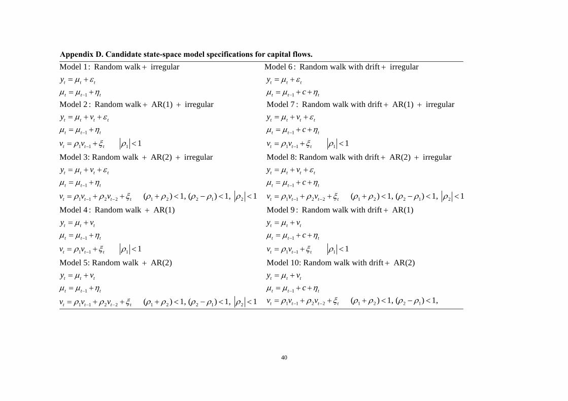
40

Appendix D. Candidate state-space model specifications for capital flows.

1

1

1 1 1

1

1

Model 1: Random walk irregular

Model 2 : Random walk AR(1) irregular

1

Model 3: Random walk AR(2) irregular

t t t

t t t

t t t t

t t t

t t t

t t t t

t t t

t

y

y v

v v

y v

v

1 2 2 1 2 2 1 2

1

1 1 1

1

1 1 2 2 1 2 2

( ) 1, ( ) 1, 1

Model 4 : Random walk AR(1)

1

Model 5: Random walk AR(2)

( ) 1, (

t t t

t t t

t t t

t t t

t t t

t t t

t t t t

v v

y v

v v

y v

v v v

1

1

1 1 1

1 2

Model 6 : Random walk with drift irregular

Model 7 : Random walk with drift AR(1) irregular

1

Model 8: Random walk wi

) 1, 1

t t t

t t t

t t t t

t t t

t t t

y

c

y v

c

v v

1

1 1 2 2 1 2 2 1 2

1

1 1 1

th drift AR(2) irregular

( ) 1, ( ) 1, 1

Model 9 : Random walk with drift AR(1)

1

Model 10:

t t t t

t t t

t t t t

t t t

t t t

t t t

y v

c

v v v

y v

c

v v

1

1 1 2 2 1 2 2 1

Random walk with drift AR(2)

( ) 1, ( ) 1,

t t t

t t t

t t t t

y v

c

v v v