Analyses of wildlife-vehicle collision data: applications for guiding decision-making for wildlife crossing mitigation and

motorist safety

II. Methods and applications - Hotspot identification of wildlife-vehicle collisions for transportation planning

by

Dr. Anthony P. Clevenger Research Wildlife Biologist

& Amanda Hardy, M.Sc.

Research Scientist - Ecologist

Western Transportation Institute College of Engineering

Montana State University – Bozeman

Kari Gunson Research Scientist

College of Environmental Science & Forestry Syracuse University, Syracuse, New York

A work scope prepared for

Dr. John Bissonnette and the National Cooperative Highway Research Program Utah State University

May 28, 2006

0

CONTENT 1. INTRODUCTION Problem statement

Purpose of report 2. METHODOLOGICAL APPROACH Study area

Canadian Rocky Mountains Northern California

Mapping Techniques 1. Hotspot identification and patterns for one species and landscape

1.A. Simple graphic techniques, one dataset Visual analysis and observation of UVC patterns

1.B. Analytical techniques, one dataset Linear nearest neighbor analysis index Cluster analysis-nearest neighbor hierarchical techniques Ripley’s K analysis Density measures- UVCs per mile segment

2. Comparison of hotspot identification techniques Visual analysis and observation vs analytical techniques Crimestat vs Density-based techniques

3. Hotspot identification and patterns for different species and landscapes

3. GIS LINKAGES TO HOTSPOT DATA Bridge rebuilding projects State transportation planning Landscape and road features

4. GUIDELINES FOR WVC HOTSPOT APPLICATIONS 5. LITERATURE CITED

1

1. INTRODUCTION

Problem statement Wildlife-vehicle collisions (WVCs) are a significant problem in North America, particularly in rural or suburban areas where people rank them as a major safety concern. A recent survey of motorists in Montana, Idaho, and Wyoming placed animals on the roadway as one of the top three safety issues (Farrell et al. 2002). A survey of Northern California and rural Oregon stakeholders reported similar concerns. In much of the Western United States, road networks are extensive and motor vehicle use has sharply increased as wild lands are progressively developed and suburbanized (Benfield et al. 1999, Hansen et al. 2002). The human and infrastructure expansion that many states and municipalities are experiencing, in association with increasing wildlife populations in some areas, has led to greater safety concern and need to develop effective countermeasures to mitigate WVCs. In 2002, there were more than 1.5 million WVCs resulting in 150 fatalities and $1.1 billion dollars in vehicle damage (Hedlund et al. 2003). Studies of WVCs have demonstrated that they are not random occurrences but are spatially clustered (Puglisi et al., 1974; Hubbard et al., 2000; Clevenger et al., 2001; Joyce and Mahoney, 2001). However, there are few studies that specifically address the nature of WVC hotspots or their use and application in transportation planning (Lloyd and Casey 2005, Kasser and Bissonette 2005). These studies have been spatially explicit and utilized one method of determining hotspot locations. Many of the studies characterizing WVCs have appeared in scientific and management-focused journals, which often culminate in a variety of conclusions or recommendations for managers to consider in designing wildlife-friendly highways (Puglisi et al. 1974, Hubbard et al. 2000, Nielsen et al. 2003, Malo et al. 2004). However, what is sorely lacking are best management practices for identifying WVC hotspots based on current knowledge and technology to help guide planning and decision-making. Because WVCs represent a distribution of points, clustering techniques can be used to identify hotspots. Simple plotting of WVC location points can be done in a variety of geographic information system (GIS) formats, for example ArcView® or ArcGIS® (ESRI 1999, 2003), currently being used by many transportation agencies. Simple plotting does not require statistical algorithms or metrics, but is based on visual groupings of road-kill clusters and decision-based rules of defining hotspots. Clustering of WVCs has been correlated to animal distributions, abundances, dispersal habits, and road-related factors including local topography, vegetation, vehicle speed, and fence location or type (Puglisi et al., 1974; Allen and McCullough, 1976; Case, 1978; Clevenger et al., 2001).

Purpose of report In this report we investigate various WVC hotspot identification (clustering) techniques that can be used in a variety of landscapes, taking into account different scales of application and transportation management concerns (e.g., motorist safety, endangered species management). We obtained WVC datasets from two locations in North America with varying wildlife communities, landscapes and transport planning issues. We demonstrate how this information can be used to identify WVC hotspots at different scales

2

of application (from project level to state level analysis). Some clustering techniques that we will demonstrate include Ripley’s K-statistic of road-kills, nearest-neighbor measurements, density measures, and provide an overview of software applications that facilitate these types of analyses. The use of GIS-based information linked to hotspot data will also be addressed. Using demonstrated methods, results, and applications of results; we will develop guidelines for the use, analysis, and applications of WVC data for transportation planning practices. Overall the information we present in this report will advance our understanding of the considerations that must be taken into account when analyzing WVC datasets of varying qualities and scales. Results from this effort will help agencies hone their WVC data collection techniques and analytical techniques in order to yield more accurate and useful information that can be used to mitigate negative impacts related to wildlife-transportation conflicts. The work will complement the growing body of research on how to mitigate road impacts to wildlife and improve highway safety. Lastly, it will provide practitioners and managers with methods that can be quickly applied to available information and ultimately streamline the delivery of transportation projects in areas where WVCs are a major concern to agencies and stakeholders.

2. METHODOLOGICAL APPROACH Simple plotting of animal-vehicle collisions can be done in a variety of GIS formats, for example ArcView® or ArcGIS®, currently being used by many transportation agencies. Simple plotting does not require statistical algorithms or metrics, but is based on visual groupings of road-kill clusters and decision-based rules of defining hotspots. The primary objective of this task is to use one WVC dataset (ungulate-vehicle collisions [UVCs]s in Canadian Rocky Mountains) to demonstrate how this readily available information can be used by transportation agencies to identify WVC hotspots and different scales of application (project level to state level analysis). Study area Canadian Rocky Mountains This study took place in the Central Canadian Rocky Mountains in western Alberta approximately 100 km west of Calgary (Figure 1). The area encompasses the Bow River watershed comprising mountain landscapes in Banff National Park and adjacent Alberta Provincial lands in Kananaskis Country. Topography is mountainous, elevations range from 1,300 m to over 3,400 m, and valley floor width varies from 2-5 km. Highways in the study area traverse montane and subalpine ecoregions through four major watersheds in the region. Table 1 describes the location and general characteristics of the five segments of highways that were included in this study. The Bow River Valley is situated within the front and main ranges of the Canadian Rocky Mountains. The roads in this study traversed montane and subalpine ecoregions. Vegetation consisted of open forests dominated by Douglas fir Pseudotsuga menziesii, white spruce

3

Picea glauca, lodgepole pine Pinus contorta, Englemann spruce P. englemannii, aspen Populus tremuloides and natural grasslands. Data were collected on the incidence of wildlife vehicle collisions (WVCs) on the five highways in the study area. Data were obtained from the agencies and highway maintenance contractors that were responsible for collecting and reporting WVCs. The agencies consisted of Parks Canada (Banff, Kootenay and Yoho National Parks), Alberta Sustainable Resource Development (Bow Valley Wildland Park and Kananaskis Country) and Volker-Stevin, maintenance contractor for the Trans-Canada Highway (TCH) east of Banff National Park in the province of Alberta. Cooperators included national park wardens, provincial park rangers and maintenance crews of Volker-Stevin. For this report, we only used ungulate-vehicle collision (UVC) data, because ungulate species comprised 76% of the total wildlife mortalities. In addition, these species are often the greatest safety concern to transportation agencies given their size and relatively common occurrence in rural and mountainous landscapes. Ungulate species included white-tailed and mule deer (Odocoileus virginianus and O. hemionus, respectively), unidentified deer species, elk (Cervus elaphus), moose (Alces alces), and bighorn sheep (Ovis canadensis). Northern California This study took place in Sierra County, California in the Sierra Nevada Mountains (Figure 2). We used 849 deer carcass locations collected along 33 miles of California State Highway (SH) 89. The Highway runs along the east side of the Sierra Nevada Mountains from the towns of Truckee to Sierraville. The California Department of Transportation (hereafter referred to as Caltrans) has consistently collected deer carcass data on this highway from June 1979 to October 2005. The data were collected by maintenance supervisors and varies in spatial accuracy from the closest 1.0-mile, 0.1-mile, and 0.001-mile. The highway is a two-lane undivided highway with AADTV of 2250 and peaks at 3300 in the summer months. Elevation ranges from 6150 feet surrounding the southern most section of highway (mile 11.0) to 5081 feet in the northern section. The dominant vegetation is ponderosa pine (Pinus ponderosa) bitterbrush (Purshia tridentata) and sagebrush (Artemisia tridentata). The area receives relatively less precipitation then in the west as it is located in a rainshadow. Winter months can have up to 2 to 3 feet of snowfall. (Sandy Jacobson, personal communication). The SH 89 bisects an important migration route for the Loyalton-Truckee mule deer (Odocoileus hemionus) herd, which travel across the highway during upslope and downslope seasonal migrations. Further the highway bisects the home ranges of numerous resident deer and is important for forest carnivores and amphibians.

4

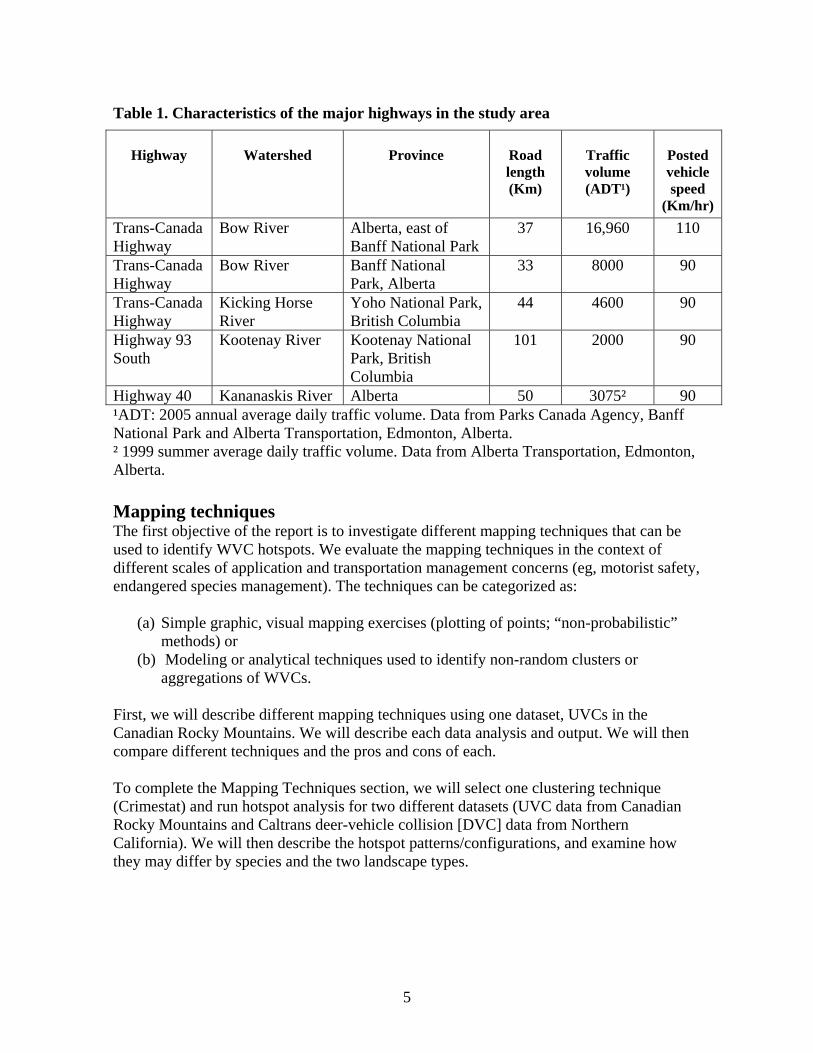
Table 1. Characteristics of the major highways in the study area

Highway Watershed Province Road length (Km)

Traffic volume (ADT¹)

Posted vehicle speed

(Km/hr) Trans-Canada Highway

Bow River Alberta, east of Banff National Park

37 16,960 110

Trans-Canada Highway

Bow River Banff National Park, Alberta

33 8000 90

Trans-Canada Highway

Kicking Horse River

Yoho National Park, British Columbia

44 4600 90

Highway 93 South

Kootenay River Kootenay National Park, British Columbia

101 2000 90

Highway 40 Kananaskis River Alberta 50 3075² 90 ¹ADT: 2005 annual average daily traffic volume. Data from Parks Canada Agency, Banff National Park and Alberta Transportation, Edmonton, Alberta. ² 1999 summer average daily traffic volume. Data from Alberta Transportation, Edmonton, Alberta. Mapping techniques The first objective of the report is to investigate different mapping techniques that can be used to identify WVC hotspots. We evaluate the mapping techniques in the context of different scales of application and transportation management concerns (eg, motorist safety, endangered species management). The techniques can be categorized as:

(a) Simple graphic, visual mapping exercises (plotting of points; “non-probabilistic” methods) or

(b) Modeling or analytical techniques used to identify non-random clusters or aggregations of WVCs.

First, we will describe different mapping techniques using one dataset, UVCs in the Canadian Rocky Mountains. We will describe each data analysis and output. We will then compare different techniques and the pros and cons of each. To complete the Mapping Techniques section, we will select one clustering technique (Crimestat) and run hotspot analysis for two different datasets (UVC data from Canadian Rocky Mountains and Caltrans deer-vehicle collision [DVC] data from Northern California). We will then describe the hotspot patterns/configurations, and examine how they may differ by species and the two landscape types.

5

1. Hotspot identification and patterns for one species and landscape 1.A. Simple graphic techniques, one dataset Visual analysis and observation of UVC patterns Methods. We obtained the Universe Transverse Mercator (UTM) coordinates using a geographic positioning system (GPS) unit for over 500 spatially accurate locations (<3 m error) of UVCs between 1997 and 2004 in the Canadian Rocky Mountains. We used the UTM Nad 83 location to plot all of the UVC data within ArcGIS 9.0 on the highway network. We derived the hillshade rastar dataset from the digital elevation model (DEM) and used this as a backdrop layer for visual interpretation. Results and Discussion. A total of 546 UVC observations were recorded between August 1997 and November 2003 on all five highways in the study area (Figure 3). Deer (mule deer, white-tailed deer and unidentified deer) were most frequently involved in collisions comprising 58% of the kills, followed by elk (27%), moose (7%) Rocky Mountain bighorn sheep (3%) and “other ungulates” (including mountain goats Oreamnos americanus), unknown species of ungulates (5%). The majority of UVCs occurred on the TCH east of Banff National Park in the province of Alberta (46%), followed by Highway 93 South in Kootenay National Park (22%), Highway 40 in Kananaskis Country (12%), the TCH in Yoho National Park (10%), and the TCH in Banff National Park (10%). A simple visual analysis of the UVC locations is shown in Figure 3. It becomes obvious that a simple plotting of all UVC locations along highways does not clearly identify key areas where UVC occur or areas of higher than average densities of collisions – at least in this type of mountainous landscape that characterizes the study area. Simple plotting of UVC locations results in collision points being tightly packed together, in some cases directly overlapping with other or close neighboring UVC locations, thus making it difficult to identify where the real high-risk collisions areas occur. This approach does allow one to see where the bulk of UVC occur and stretches of highway where few or no UVC occur. The use of a DEM and/or land cover map overlay does provide readily information on the juxtaposition of UVCs to terrain features (lowlands, lakes, steep terrain, vegetation cover types, etc). A visual analysis can provide some cursory conclusions about why and where UVCs tend to occur most. However, even with these two baseline data maps a more rigorous spatial analysis can be carried out to summarize or test statistically the ‘why and where’ questions. Terrain and habitat are often key factors influencing where UVCs occur (Bashore et al. 1985, Malo et al. 2004, Biggs et al. 2004). The type of terrain and landscape mosaic would be expected to influence UVC hotspot clustering patterns. For example, landscapes with homogeneous cover types with little topographic relief (ie, flat terrain) would likely result in a random-like pattern of movement across a highway, and thus collision locations on a

6

given stretch of highway. The contrary, being a highly heterogeneous landscape with dissected topography should result in more clearly defined crossing locations and collision hotspots. The factors that contribute to these collisions will be different in both landscapes. More simplistic models with fewer explanatory variables would characterize the level, homogeneous landscape, whereas more complex models with numerous variables in the more diverse landscape. This should provide thought for future syntheses of information causing collisions and how landscape diversity might affect their causes and ultimately spatial distribution. 1.B. Analytical techniques, one dataset Linear nearest neighbor analysis index All UVCs were plotted for each highway on the highway network layer in ArcGIS 9.0. We used Hawths Analysis Tools (Beyer 2004) extension to generate the same number of “random UVCs” as there were actual (observed) on each highway. We used a first order linear nearest neighbor index (NNI) to evaluate if the distribution of the observed UVCs in each region of the Canadian Rocky Mountains differed from a random distribution. The index is a ratio between the mean nearest distance to each UVC (d(nn)) and the mean nearest distance that would be expected by chance (d(ran)), see Equation 1. To do this we used Hawth’s Analysis Tools to calculate d(nn) and d(ran). (1)

NNI=d(nn)/d(ran)

If the observed mean distance is smaller than the random mean distance then the UVCs occur closer together than expected by chance and NNI<1. Once tabulated all data were imported into Microsoft Excel where we calculated a Z-statistic, adapted from Clark and Evans (1954), to test whether there was a significant difference between random and observed distances. Results and Discussion. The nearest neighbor index showed clustering (NNI<1) for all highway regions except for the TCH in Yoho, which showed evidence of dispersion (Table 2). The Z-statistic was significant (p<0.05) for the TCH in Alberta and kills on Highway 93 South were marginally significant (p=0.066).

7

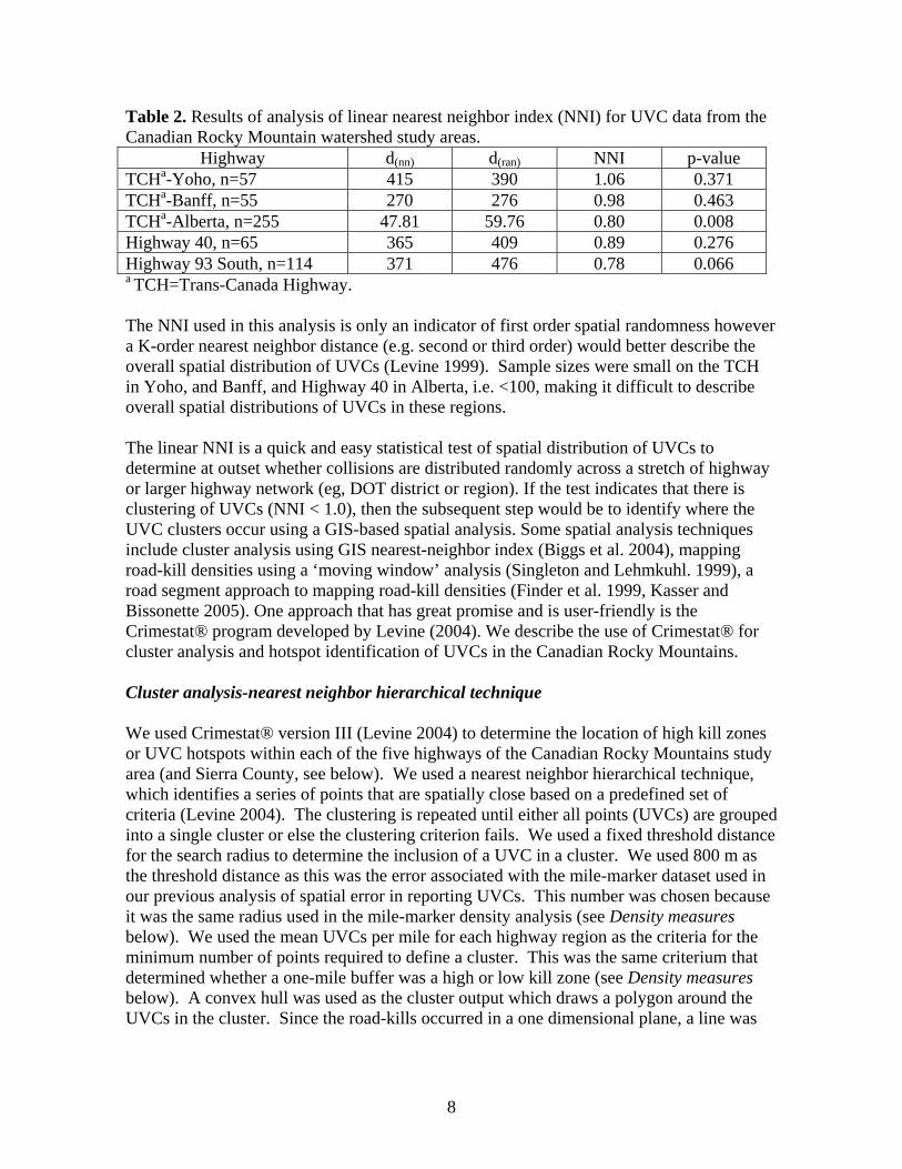
Table 2. Results of analysis of linear nearest neighbor index (NNI) for UVC data from the Canadian Rocky Mountain watershed study areas.

Highway d(nn) d(ran) NNI p-value TCHa-Yoho, n=57 415 390 1.06 0.371 TCHa-Banff, n=55 270 276 0.98 0.463 TCHa-Alberta, n=255 47.81 59.76 0.80 0.008 Highway 40, n=65 365 409 0.89 0.276 Highway 93 South, n=114 371 476 0.78 0.066 a TCH=Trans-Canada Highway. The NNI used in this analysis is only an indicator of first order spatial randomness however a K-order nearest neighbor distance (e.g. second or third order) would better describe the overall spatial distribution of UVCs (Levine 1999). Sample sizes were small on the TCH in Yoho, and Banff, and Highway 40 in Alberta, i.e. <100, making it difficult to describe overall spatial distributions of UVCs in these regions. The linear NNI is a quick and easy statistical test of spatial distribution of UVCs to determine at outset whether collisions are distributed randomly across a stretch of highway or larger highway network (eg, DOT district or region). If the test indicates that there is clustering of UVCs (NNI < 1.0), then the subsequent step would be to identify where the UVC clusters occur using a GIS-based spatial analysis. Some spatial analysis techniques include cluster analysis using GIS nearest-neighbor index (Biggs et al. 2004), mapping road-kill densities using a ‘moving window’ analysis (Singleton and Lehmkuhl. 1999), a road segment approach to mapping road-kill densities (Finder et al. 1999, Kasser and Bissonette 2005). One approach that has great promise and is user-friendly is the Crimestat® program developed by Levine (2004). We describe the use of Crimestat® for cluster analysis and hotspot identification of UVCs in the Canadian Rocky Mountains. Cluster analysis-nearest neighbor hierarchical technique We used Crimestat® version III (Levine 2004) to determine the location of high kill zones or UVC hotspots within each of the five highways of the Canadian Rocky Mountains study area (and Sierra County, see below). We used a nearest neighbor hierarchical technique, which identifies a series of points that are spatially close based on a predefined set of criteria (Levine 2004). The clustering is repeated until either all points (UVCs) are grouped into a single cluster or else the clustering criterion fails. We used a fixed threshold distance for the search radius to determine the inclusion of a UVC in a cluster. We used 800 m as the threshold distance as this was the error associated with the mile-marker dataset used in our previous analysis of spatial error in reporting UVCs. This number was chosen because it was the same radius used in the mile-marker density analysis (see Density measures below). We used the mean UVCs per mile for each highway region as the criteria for the minimum number of points required to define a cluster. This was the same criterium that determined whether a one-mile buffer was a high or low kill zone (see Density measures below). A convex hull was used as the cluster output which draws a polygon around the UVCs in the cluster. Since the road-kills occurred in a one dimensional plane, a line was

8

drawn from the two outermost points along the road within the convex hull for visual display and to calculate the length of each UVC cluster. Results and Discussion. A total of 42 UVC clusters were produced using the nearest neighbor Crimestat® analysis and comprised 41 km of highway in the study area (Figure 4). Compared to the simple visual analysis of UVCs, the Crimestat® modeling technique effectively reduces the blurring of information associated with numerous UVCs on long stretches of highway. As mentioned earlier, simple plotting of UVC locations tends to result in tight grouping of collision points that often times overlap with other UVC locations. This spatial arrangement of UVCs makes it a challenge to identify where high-risk collisions areas actually occur. The location and number of UVC hotspots generated by the Crimestat® technique are clearly defined and can be identified with associated landscape or road-related features in each highway area. Ripley’s K analysis Ripley’s K-statistic describes the dispersion of data over a range of spatial scales (Ripley 1981; Cressie 1991). We calculated Ripley’s K-statistic for all mortalities in each region of the Canadian Rocky Mountains. We used the K-statistic as defined by Levine (1999), but modified for points distributed in one dimension (i.e. along a line or road network). The resulting algorithm was coded in Avenue TM and run in ArcView© GIS (Environmental Systems Research Institute, 1999). The algorithm counted the number of neighboring UVCs within a specified scale distance (t) of each UVC and these counts were summed over all UVCs. We standardized the UVC totals by sample size (N) and highway length (RL) to allow for comparison between each highway region. The process was repeated for incrementally larger scale distances up to RL for all five highways. The K-statistic (adapted from Levine 1999 and O’Driscoll 1998) was defined as:

KRLN

I2( )distance dobs ijj

N

ii j

N

===

≠

∑∑11

(2) ( )

Where dij is the distance from UVC i to UVC j and I(dij) is an indicator function that returns 1 if dij ≤ distance and zero otherwise (O’Driscoll 1998). We used a distance increment of 280 m for all five highway regions to allow for a minimum of 100 ds bins on the shortest section of highway (i.e. TCH-AB). To assess the significance of K-values we ran 50 simulations of equation [2] based on random distributions of points for each of the five categories. We display results as plots of L versus distance, where L is the difference between the observed K-value and the mean of the K-values for the 50 simulations (O’Driscoll 1998). Positive values of L indicate crowding and negative values indicate dispersion. We also present the 95% confidence limits calculated as the upper or lower 95th percentile of the random simulations minus the mean of the random simulations (O’Driscoll 1998). We defined significant crowding as

9

any value of L above the upper confidence limit and significant dispersion as any value of L below the lower confidence limit. Results and Discussion. Neighbor K statistics are well suited for the description of 1-dimensional spatial distributions (Ripley, 1981; Getis and Franklin, 1987; Ramp et al. 2005). The range of scales over which clustering appears significant is dependent on the intensity of the distribution of road-kills (Clevenger et al. 2003, Ramp et al. 2005). The distribution of UVCs was heterogeneous and significantly more clustered or dispersed than would be expected by chance over a wide range of scales (p<0.05, Figure 5). In all highway regions there was significant clustering of UVCs and some significant dispersion. The TCH inYoho had a small degree of clustering from 1 to 2 km at an intensity of 0.3 km, and significant dispersion at spatial scales from 3–12 km and 18–45 km. This dispersion peaked at an intensity of 7 km. This small scale of clustering can be seen at the westernmost section of the Highway in Figures 3 and 4. Peaks in L(t) or the intensity of clustering occurred between km 4 and 5 for the TCH in Alberta and the TCH in Banff. This means there was an average of 4–5 extra neighbors within the scale distance of 0 to 10 km on the TCH in Banff and 0-12 km in Alberta. Both these aggregations can be seen in Figures 2 and 3. In Banff it corresponds with the section of TCH that bisects a North-South aligned major drainage. At large scale distances the TCH in BNP and Alberta show a random distribution with small scales of dispersions. On Highway 93 South there is a large peak (27 extra neighbors) in UVC clustering at a scale distance of 0 to 80 km. This corresponds to the bulk of the UVCs occurring at the southernmost section of Highway in low elevation montane habitat. Further, the Highway bisects a key ungulate movement corridor in this area. The Ripley’s K analysis clearly shows the spatial distribution of UVCs along each segment of highway. The large-scale aggregation evident on Highway 93 South in Kootenay shows the importance of broad scale landscape variables such as elevation and valley bottoms in a mountain environment. The scale of UVC aggregations in each study area can be used to help determine the scale and type of variables to be used in explaining the occurrence of road mortality of wildlife. Further, the locations of high intensity road-kill clustering within each aggregation can help to focus or prioritize the placement of mitigation activities, such as wildlife crossings or other countermeasures, on each highway segment. Density measures - UVCs per mile segment For the next two analyses we used the mile-marker data generated in our earlier report on the limiting effects of road-kill reporting data due to spatial inaccuracy. We divided each of the five highways in the Canadian Rocky Mountain study area into 1.0 mile-marker segments and plotted all spatially accurate UVC data onto each road network and then moved each point (UVC) to the nearest mile-marker reference point. We recorded the UTM coordinates of each mile-marker location, and summed the number of UVCs in that

10

mile-marker segment, defined as 800 m (0.5 mile) up- and down-road of the given mile-marker location. A. Graduated or weighted mile kill categories We weighted each mile-marker by the summed number of UVCs associated with it and used graduated symbols in Arcview 3.3 to display UVCs along each highway region. A 1:50,000 DEM, pixel size 30 m x 30 m was used to derive the hillshade (GIS database management, Banff National Park) for the highways in the study area and used as a backdrop for visualization. A. Results and Discussion. Figure 6 effectively shows where the UVCs are occurring in relation to the valleys and rugged terrain of the Rocky Mountain landscape. The black arrows in the figures indicate where there is a large clustering of UVCs, which generally is where the highway bisects a valley bottom. The TCH in Alberta is a consistent stretch of UVCs (14-24 road-kills at each mile-marker) from the Banff National Park east boundary to just west of Highway 40. The first westernmost gap in mortality numbers (indicated by the star symbol) is due to the presence of 4.5 km of fenced highway with one underpass, while the second gap in UVCs is due to a large lake and river system on the north side of the TCH. B. High kill and low kill categories We categorized each mile-marker segment as a “high kill” or “low kill” zone by comparing the summed number of UVCs associated with a single mile-marker segment to the average number of UVCs per mile for the same stretch of road, for each of the five highways in the study area. If the summed number of UVCs associated with a single mile-marker segment was higher than the average calculated per mile for the same highway, that mile-marker segment was considered a “high kill zone”. Similarly, if the summed number of UVCs within a mile-marker segment was lower than the average for that highway, the mile-marker segment was listed as a “low kill zone”. Each low and high kill zone or buffer was color-coded and displayed on each highway segment along with the associated lakes layer. Other features in the landscape, such as human use and rivers were not displayed because they were not visual at the given scale for each figure. The lakes layer was digitized from 1:50,000 topographic maps and only displayed within a 800 m buffer around each highway in each region. In order to compare the level of aggregation of high kill zones between highway regions we measured the mean length of each high kill aggregation. A high kill aggregation was defined as a high kill zone (buffer) with at least one neighboring high kill zone. All spatial analyses were conducted in Arcview 3.3 and ArcGIS 9.0 and statistical analyses were conducted in Microsoft Excel 2000. A DEM with a pixel size 30 m x 30 m was used to derive the hillshade (GIS database management, Banff National Park, U.S. Geological Surveys) for the Canadian Rocky Mountain and used as a backdrop for visualization. B. Results and Discussion. When taking into account roadway length the majority of UVCs occurred on the TCH in Alberta (13.5 road-kills/mile), followed by the TCH in

11

Banff (2.6 road-kills/mile), the TCH in Yoho (2.1 road-kills/mile), Highway 40 (2.1 road-kills/mile) and Highway 93 South (1.8 road-kills/mile). These rates of UVC were used to determine high and low kill segments in each highway region. This analysis produced 97.6 km of high kill zones on all highways in the study area (Figure 7). In 52% of the cases a high kill zone had a neighboring high zone. Highway 93 South had the most high kill zones; however the TCH in Banff had the highest mean length of aggregated high kill zones, while the TCH in Yoho had the lowest mean length of high kill zones (Table 3). The standard deviations on TCH-BNP was high indicating the size of aggregations highly fluctuated. Figure 7 shows one main aggregation and a few single high zones on the TCH in Banff. In both the mile-marker visualizations (Figures 6 & 7) the DEM backdrops easily show that high kills zones are associated with valleys moving perpendicular to the direction of the highway. For example the highway where a large aggregation (~13 km) of high kill zones on Highway 93 South in Kootenay National Park bisects key ungulate ranges in the valley bottoms of the montane region, with elevation less than 1240 m. 2. Comparison of hotspot identification techniques Visual analysis and observation vs analytical techniques The pros and cons of the simple visual analysis of UVC vs more complex or analytical methods were discussed earlier (see Discussion of 1.A. Simple graphic techniques, one dataset). Essentially with simple plotting of UVCs there will be a tendency for road-kill points to overlap and actually mask the importance of segments of highway that have high density of UVCs. Modeling or analytical techniques permit a more detailed assessment of where UVCs occur, their intensity and means to begin prioritizing highway segments for potential mitigation applications. Last, the identification and delineation of UVC clusters, which can vary widely in length depending on distribution and intensity of collisions, facilitates between-year or multiyear analyses of the stability or dynamics of UVC hotspot locations. Crimestat vs Density-based techniques Using the nearest neighbor Crimestat® analysis 42 UVC clusters were produced and combined occupied a total of 41 km (15%) of highway in the study area. The nearest neighbor Crimestat® technique was more conservative compared to the mile-marker density analysis by identifying less length of highway as a UVC hotspot. The average length of UVC clusters was smaller than the density-based high-kill aggregations; however the Crimestat® analysis produced clusters that were not continuous (Table 3). If we had selected a larger search radius for inclusion of road-kill points the UVC clusters we would have had fewer clusters. Crimestat® also consistently produced fewer clusters of UVCs than the mile-marker density analysis. Use of either technique for identifying UVC or road-kill hotspots may depend on the management objective. The Crimestat® approach is useful for identifying key hotspot areas

12

on highways with many road-kills and through simple visual analysis appears they are more or less continuously distributed. In essence filtering through the road-kill data to extract where the most problematic areas lie. The mile-marker density analysis results in identifying more hotspot clusters on larger sections of highway. Although this approach appears to be less useful to management, it may be a preferred option where managers are interested in taking a broader, more comprehensive view of wildlife-vehicle conflicts within a given area. This may be necessary to not only prioritize areas of conflicts but plan a suite of mitigation measures (eg, placement of a wildlife crossing vs fencing vs lighting). The location of the larger clusters produced by the density analysis could be tracked each year to determine how stable they are or whether there is a notable amount of shifting between years or over longer time periods. This type of information will be of value to managers in addressing the type of mitigation and intended duration (eg, short-term vs. long-term applications). The clusters followed a similar spatial distribution as the mile-marker high kill zones (Figure 4). The degree of overlap between the two techniques was high for 3 of the 5 highways. For example all the clusters on the TCH-Yoho fell within high-kill zone aggregations (Table 3). Similar patterns of overlap were found for the TCH in Alberta and Highway 40 in Kananaskis Country. Less overlap of clusters defined by the two techniques was found for Highway 93 South and the TCH in Banff. The above results beg the question, what mechanisms influence the spatial patterns of clusters derived by both techniques? Why is cluster overlap high in some areas, but low in others? Both techniques coincided perfectly on the TCH in Yoho (100% overlap), whereas they were most divergent on Highway 93 South in Kootenay National Park (roughly 50% overlap). The overlap of clusters on the other three highways was either aligned with one of the two endpoints above. From inspection of the UVC data on all five highways we suggest that the amount of UVC cluster overlap from the two techniques is likely influenced by the density and distribution pattern of UVCs. High overlap was found on the TCH in Yoho, where steep terrain dictates more or less where animals can cross the highway. There are few suitable locations where wildlife can cross the TCH, thus road-kills occur in clearly defined sections. Clusters will naturally overlap or be in proximity since collisions rarely occur outside the key highway crossing areas. On highways that have less topographic constraints and more dispersed wildlife habitat, UVCs will tend to be greater in number and more uniformly distributed than on the Yoho highway. Cluster definition will tend to diverge, some overlapping but largely clusters from the two approaches will become spatially isolated. The reason being the density-based method has a tendency to accommodate outlying or marginal UVCs that normally would not cluster using Crimestat®.

13

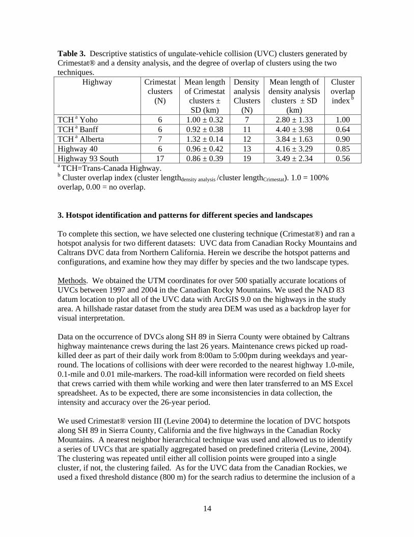
Table 3. Descriptive statistics of ungulate-vehicle collision (UVC) clusters generated by Crimestat® and a density analysis, and the degree of overlap of clusters using the two techniques.

Highway Crimestat clusters

(N)

Mean length of Crimestat

clusters ± SD (km)

Density analysis Clusters

(N)

Mean length of density analysis clusters ± SD

(km)

Cluster overlap index b

TCH a Yoho 6 1.00 ± 0.32 7 2.80 ± 1.33 1.00 TCH a Banff 6 0.92 ± 0.38 11 4.40 ± 3.98 0.64 TCH a Alberta 7 1.32 ± 0.14 12 3.84 ± 1.63 0.90 Highway 40 6 0.96 ± 0.42 13 4.16 ± 3.29 0.85 Highway 93 South 17 0.86 ± 0.39 19 3.49 ± 2.34 0.56 a TCH=Trans-Canada Highway. b Cluster overlap index (cluster lengthdensity analysis /cluster lengthCrimestat). 1.0 = 100% overlap, 0.00 = no overlap. 3. Hotspot identification and patterns for different species and landscapes To complete this section, we have selected one clustering technique (Crimestat®) and ran a hotspot analysis for two different datasets: UVC data from Canadian Rocky Mountains and Caltrans DVC data from Northern California. Herein we describe the hotspot patterns and configurations, and examine how they may differ by species and the two landscape types. Methods. We obtained the UTM coordinates for over 500 spatially accurate locations of UVCs between 1997 and 2004 in the Canadian Rocky Mountains. We used the NAD 83 datum location to plot all of the UVC data with ArcGIS 9.0 on the highways in the study area. A hillshade rastar dataset from the study area DEM was used as a backdrop layer for visual interpretation. Data on the occurrence of DVCs along SH 89 in Sierra County were obtained by Caltrans highway maintenance crews during the last 26 years. Maintenance crews picked up road-killed deer as part of their daily work from 8:00am to 5:00pm during weekdays and year-round. The locations of collisions with deer were recorded to the nearest highway 1.0-mile, 0.1-mile and 0.01 mile-markers. The road-kill information were recorded on field sheets that crews carried with them while working and were then later transferred to an MS Excel spreadsheet. As to be expected, there are some inconsistencies in data collection, the intensity and accuracy over the 26-year period. We used Crimestat® version III (Levine 2004) to determine the location of DVC hotspots along SH 89 in Sierra County, California and the five highways in the Canadian Rocky Mountains. A nearest neighbor hierarchical technique was used and allowed us to identify a series of UVCs that are spatially aggregated based on predefined criteria (Levine, 2004). The clustering was repeated until either all collision points were grouped into a single cluster, if not, the clustering failed. As for the UVC data from the Canadian Rockies, we used a fixed threshold distance (800 m) for the search radius to determine the inclusion of a

14

collision point in a cluster. We used the average number of DVCs per mile on SH 89 as the criteria for the minimum number of points required to identify a DVC cluster. A convex hull was used as the cluster output which draws a polygon around the collision points in the cluster. Since road-kill data occurs in a one-dimensional plane, a line was drawn from the two outermost points along the highway within the convex hull for visual display and to calculate the length of each cluster. Results and Discussion. For visual comparisons we also did a simple visual plotting of all DVC data along SH 89 in Sierra County, California. The dataset was comprised of 849 DVCs from June 1979 to October 2005. (Figures 8). The mean number of DVCs was 25.7 kills/mile for the 26-year period. All things being equal, this equates to roughly 1 kill recorded per mile per year. There is a high amount of overlap of DVC points on SH 89 based on the simple plotting of collisions. Like the simple plots made of UVCs in the Canadian Rocky Mountains it is difficult to identify where hotspot actually occur. The excessive overlap and what appears to be continuous clustering of DVC points is most likely a result of the high number and density of DVCs for a relatively short stretch of highway. Note that the California DVC data were obtained from a 26-year period, compared to 500+ points from the Canadian study area, obtained from >250 km of highway during a 7-year period. Crimestat® clusters were only created on the 18 km southern section of Highway 89 because the majority of the DVCs occurred on this section. The Crimestat-generated clusters occupied a large proportion of the highway, more than half of the 18 km section. Hotspots were associated with a variety of terrain types, but largely with mountainous terrain. Some of the hotspot clusters appear to be associated with valley bottom habitats, but a substantial amount can be linked with river courses in rugged terrain. Given the large number of hotspots identified along SH 89 management would need to prioritize which ones were real safety and wildlife conservation concern. The large 26-year dataset clouds the picture by having numerous DVCs on one stretch of highway. A sequential analysis of DVC hotspots in 5-year increments would help identify trends and patterns in hotspot distribution and bring to light the more problematic sections of highway for motorists and wildlife. State Highway 89 Northern California and Highways in the Canadian Rocky Mountains The Crimestat® analysis of SH 89 produced 9 clusters with a mean length of 1.34 ± 0.26 km (Table 4). This average length is similar but slightly greater (330 m) than the clusters produced in the Canadian Rocky Mountains. Although hotspot clusters were similar in length in both areas, the density, pattern and landscape attributes were distinct between both areas. Both areas are characterized by rugged mountainous terrain, however, the majority of hotspots clusters in the Canadian Rockies were associated with wide, montane, valley bottom habitats. Where highways traversed upper sections of watersheds or bisected mountain passes, few UVC hotspots occurred. The observed differences in hotspot associations with biophysical factors such as terrain and other landscape features may be best explained by the habitat and movement requirements of mule deer (SH 89) and elk (primary species in UVCs in Canadian Rockies). Interestingly there are relatively large

15

sections of SH 89 where no DVC hotspots were identified. It would be interesting to know how land cover, terrain and other biophysical features differ in these segments compared to the DVC hotspots. To further understand these spatial patterns of DVC hotspot distribution a preliminary analysis using readily available GIS data layers can help evaluate the importance of landscape, habitat and road features associated with each hotspot. The following section addresses some ways that can be conducted. Table 4. Descriptive statistics of the Crimestat® clusters delineating deer-vehicle collision hotspot clusters on State Highway 89, Sierra County, California.

Highway Number of clusters

Mean cluster length ± SD (km)

Highway 89 9 1.34 ± 0.26

3. GIS LINKAGES TO HOTSPOT DATA The collection of animal-vehicle collision data is important for many reasons, but more than anything serves as baseline information to guide the planning and future management of roadways. Animal-vehicle collision data can be used to quickly identify at a coarse scale where problematic areas lie on roads, much like we have demonstrated with several of the techniques shown above. This may help efficiently guide planning and decision-making if transportation improvement plans encompass designated WVC hotspots. Our research approach to address the issues, assumptions, and techniques that can be used to analyze and apply WVC data with the goal of reducing wildlife-transportation conflicts is outlined below. The second objective of the report is to explore ways GIS-based information can be linked to hotspot data and their applications. With the hotspot data collected, stored in a database format, the next logical step is look at the types of GIS data that can be used to perform analyses for transportation management. These include coarse scale or preliminary analyses that can be used in rapid assessments to identify wildlife-transportation conflicts or streamlining of wildlife and safety needs in transportation planning. They can be considered a preliminary analysis because often times they are not comprehensive or statistically rigorous approaches, but rather are initial examinations of the relationships between animal-vehicle collisions and the natural and man-made environment around them. The type of data needed to identify the location of hotspots for animal-vehicle collisions need not be spatially accurate, because mitigation measures usually are focused to address problematic areas that cover several miles of highway. For this reason, data accurate to the 1.0 mile-marker is sufficient. Existing agency road-kill data can be useful for coarse-scale mapping to identify problematic areas and benefit from planned infrastructure improvement capital. Bridge rebuilding projects Bridge rebuilding and retrofits are perfect examples where hotspot information can be utilized to identify areas where highway improvement projects can improve motorist safety

16

and habitat connectivity for wildlife. The periodic reconstruction of highway bridges that span over waterways is an excellent opportunity to benefit from structural work projects to improve wildlife (and fish) passage along riparian corridors by widening bridge spans or habitat enhancement (Forman et al. 2003). State transportation planning Today, state transportation planning exercises such as STIP (Statewide Transportation Improvement Program) are identifying key areas for transportation infrastructure investments. At the same time, state natural resource agencies are mandated by Congress to develop comprehensive wildlife conservation plans that address a full array of wildlife and habitat conservation issues (Anonymous 2004). Coordination of both network plans in a timely and integrated fashion would be a significant contribution to streamlining environmental concerns in transportation planning. A recent example of integrating agency road-kill information with standard GIS data for sustainable transportation planning took place in Vermont (Austin et al. 2006). The transportation department (VTrans) developed a centralized database of wildlife road-kills, wildlife road crossing, and related habitat data for individual species throughout the state. In order to expand and improve wildlife road-kill reporting data, a partnership and recording procedures were developed with VTrans field and district staff enabling them to record a new array of wildlife road-kill information. With their wildlife road-kill information they performed a GIS-based “Wildlife Linkage Habitat Analysis” using landscape scale data to identify or predict the location of potentially significant Wildlife Linkage Habitats (WLH) associated with state roads throughout Vermont. The project relied on readily available GIS data including: (a) land use and land cover data, (b) data on developed or built areas, and (c) contiguous or “core” habitat data; these were obtained from the University of Vermont. The components that comprised of the overall GIS data layers were then ranked in accordance with their relative significance to creating potential WLH. The analysis, in conjunction with the newly updated wildlife road-kill data, provided a science-based, planning tool that will aid VTrans in understanding, addressing and mitigating the effects of roads on wildlife movement, mortality, habitat and public safety early in the design process for transportation projects. There are a variety of GIS modeling approaches today, from simple such as the one taken in Vermont to more complex models requiring high-resolution and spatially-explicit data. Most GIS modeling used in for transportation planning purposes tend to be coarse scale and do not require specially developed GIS data layers (Barnum 2001, Craighead et al. 2001, Singleton et al. 2002). Like GIS-based data on animal movements, hotspot information can be used to identify problematic areas and thus integrate mitigation where highway improvement capital will be invested. Hotspot areas that are associated with existing below-grade structures (e.g., drainage culverts and bridges) can be identified by linking GIS data, allowing structural and land planning recommendations made to improve permeability at unsuitable passage structures.

17

Landscape and road features Animal-vehicle collision data were used along Interstate 90 in Washington State to evaluate the relationship between hotspot clusters and important landscape characteristics (Singleton and Lehmkuhl 2000). The mapped road-kill density using the approach we described earlier, classifying segments as high, moderate, or low ungulate-kill density. A “classification tree analysis” (using S-Plus 2000) was used to determine the importance of 10 landscape-scale variables (GIS layers comprising road and landscape features) in the study area. Classification tree analysis is well suited for analysis of GIS spatial data. Being a nonparametric technique, it involves no assumptions of normal distribution, works well with categorical data, and is robust to the relatively subjectively determined sample sizes inherent with GIS raster data. Further, linking these coarse scale hotspots with environmental data (e.g., terrain, habitat suitability, zones of animal movement) can provide a relatively quick and reliable project-level or district-level assessment of how to prioritize mitigation activities directed at animal-vehicle collisions.

4. GUIDELINES FOR WVC HOTSPOT APPLICATIONS The last objective of the report is to develop some guidelines for the use, data analysis, application, and interpretation of results for transportation planning practices. This section will draw on the key points of the report for creating the framework. Data on hotspots of WVCs can aid transportation managers when needing to increase motorist safety, habitat connectivity for wildlife by providing safe passage across busy roadways. Knowledge of the geographic location and severity of WVCs is a prerequisite for devising mitigation schemes that can be incorporated into future infrastructure projects (bridge rebuilds, highway expansion, etc). Hotspots in close proximity to existing below-grade passage structures can facilitate structural retrofits that can help keep wildlife safely off roadways and increase habitat connectivity. The WVC data that transportation departments currently possess are suitable for meeting the primary objective of identifying hotspot locations at a range of geographic scales, from project-level (<50 km of highway) to larger district-level or statewide assessments on larger highway network systems. The spatial accuracy of WVCs is not of critical importance for the relatively coarse-scale analysis of where hotspots are located. To determine site-specific factors that contribute to WVCs, then more spatially accurate data will be required. Thus, WVCs referenced to a mile-marker system will be of sufficient quality for transportation agencies to begin identifying where problematic areas for motorists and wildlife lie on the highways they manage. WVC data with greater spatial accuracy are equally useful in determining the location of hotspots, however they are not essential to begin examining highway-wildlife conflict areas. We have outlined and described various techniques available that can help delineate WVC hotspots. Simple plotting of collision points is a relatively straightforward means of

18

identifying problematic areas, however, as sample sizes increase the tendency for road-kills to overlap (hide other points) increases. The length of highway examined, intensity of road-kills, and time period of data collection all influence the density of collision points. Other factors such as terrain, wildlife abundance and wildlife habitat quality adjacent to the highway will further affect the spatial distribution (random/continuous or non-random/clustered) of WVCs on a given highway. Modeling or analytical techniques permit a more rigorous assessment of where WVCs are likely to occur, their intensity, and means to begin prioritizing highway sections for mitigative actions. The nearest-neighbor Crimestat® method essentially pinpoints the location of WVC hotspots, whereby the segmental analysis of WVC densities provides a more comprehensive evaluation of mitigation options and prioritization of mitigation schemes based on cost-benefit, scheduling of transportation projects, or severity of motorist safety concerns. Transportation departments should continue collecting WVC data, but need to be more systematic about collection procedures. In many state agencies, WVC data collection is not consistent throughout the state and varies in intensity and data quality from district to district. Systematic data collection and protocols will allow for greater management benefits and utility of information for transportation planning and incorporating mitigation strategies in transportation projects with motorist safety and wildlife protection concerns. We are not aware of state transportation departments that have consistently used WVC hotspot data for decision-making in transportation projects or strategic planning with future infrastructure plans such as STIP in mind. The collection of WVC data systematically and comprehensively will provide important baseline information for planning and streamlining environmental mitigation in projects, and furnish critical data (pre-mitigation reference) for ultimately assessing the performance of mitigation measures that are adopted.

19

5. REFERENCES Allen, R.E. and D.R. McCullough. 1976. Deer-car accidents in southern Michigan.

Journal of Wildlife Management 40:317-325. Anonymous. 2004. Comprehensive wildlife conservation strategies state progress report #2.

March 2004. International Association of Fish and Wildlife Agencies. Washington, DC [http://www.teamingwithwildlife.org/]

Austin, J, Viani, K, and Hammond, F. 2006. Vermont wildlife habitat linkage analysis. Report to Vermont Agency of Transportation (VTrans Research Advisory Council No. RSCH008-967).

Barnum, S. 2001. Preliminary analysis of locations where wildlife crosses highways in the southern Rocky Mountians. ICOET Proceedings. pp.565-573

Bashore, T.L., Tzilkowski, W.M. and Bellis, E.D. 1985. Analysis of deer-vehicle collision sites in Pennsylvania. Journal of Wildlife Management, 49, 769-774.

Benfield, FK, Raimi, M. and Chen, DDT. 1999. Once there were greenfields. Natural Resources Defense Council. New York, NY.

Beyer, H.L. 2004. Hawth’s Analysis Tools for ArcGIS; http://www.spatial ecology.com/htools.

Biggs, J., Sherwood, S., Michalak, S., Hansen, L., and Bare, C. 2004. Animal-related vehicle accidents at the Los Alamos National Laboratory, New Mexico. The Southwestern Naturalist, 49, 384-394.

Case, R.M. 1978. Interstate highway road-killed animals: a data source for biologists. Wildlife Society Bulletin 6:8-13.

Clark, P.J. and F.C. Evans. 1954. Distance to nearest neighbor as a measure of spatial relationships in populations. Ecology. 35. 445:453.

Clevenger, A.P., Chruszcz, B. and Gunson, K. 2001. Highway mitigation fencing reduces wildlife-vehicle collisions. Wildlife Society Bulletin 29:646-653.

Clevenger, A.P., B. Chruszcz, and K. Gunson. 2003. Spatial patterns and factors influencing small vertebrate fauna road-kill aggregations. Biological Conservation 109, 15-26.

Craighead, A.C., F. L. Craighead, and E.A. Roberts. 2001. Bozeman Pass wildlife linkage and highway safety guide. ICOET Proceedings. pp 405-412.

Cressie, N. 1991. Statisitcs for Spatial Data. John Wiley and Sons, New York. Environmental Systems Research Institute (ESRI) 1999. ArcView GIS version 3.3,

Redlands, California. Environmental Systems Research Institute (ESRI) 2003. ArcGIS version 9.0, Redlands,

California. Farrell, JE, Irby, LR, McGowen, PT. 2002. Strategies for ungulate vehicle collision

mitigation. Intermountain Journal of Science 8, 1-18. Finder, R.A., Roseberry, J.L., and Woolf, A. 1999. Site and landscape conditions at white-

tailed deer-vehicle collision locations in Illinois. Landscape and Urban Planning, 44, 77-85.

Forman, R.T.T., Sperling, D., Bissonette, J., Clevenger, A., Cutshall, C., Dale, V., Fahrig, L., France, R., Goldman, C., Heanue, K., Jones, J., Swanson, F., Turrentine, T. and Winter, T. 2003. Road ecology: Science and solutions. Island Press, Washington, D.C.

20

Getis, A., Franklin, J., 1987. Second-order neighborhood analysis of mapped point patterns. Ecology 68, 473-477.

Hansen A.J.; Rasker R.; Maxwell B.; Rotella J.J.; Johnson J.D.; Parmenter A.W.; Langner U.; Cohen W.B.; Lawrence R.L.; Kraska M.P.V. 2002. Ecological Causes and Consequences of Demographic Change in the New West. BioScience 52, 151-162.

Hedlund, J.H., P.D. Curtis, G. Curtis, A.F. Williams. 2003. Methods to reduce traffic crashes involving deer: what works and what does not. Insurance Institute for Highway Safety, Arlington, VA.

Hubbard, M.W., B.J. Danielson, and R.A. Schmitz. 2000. Factors influencing the location of deer-vehicle accidents in Iowa. Journal of Wildlife Management 64:707-712.

Joyce, T.L. and S.P. Mahoney. 2001. Spatial and temporal distributions of moose-vehicle collisions in Newfoundland. Wildlife Society Bulletin 29:281-291.

Kasser, C. and J.A. Bissonette. 2005. Deer-vehicle crash hotspots in Utah: Data for effective mitigation. UTCFWRU Project report No. 2005(1): 1-128. Utah Cooperative Fish and Wildlife Research Unit, Utah State University, Logan, UT.

Levine. N. 1999. Crimestat: a spatial statistics program for the analysis of crime incident locations. Ned Levine & Associates: Annandale, Virginia and National Institute of Justice, Washington, D.C.

Levine, N. 2004. CrimeStat III: A spatial statistics program for the analysis of crime incident locations. Ned Levine & Associates: Houston, Texas, and the National Institute of Justice, Washington, D.C., USA.

Lloyd, J. and Casey, A. 2005. Wildlife hotspots along highways in Northwestern Oregon. Report to Oregon Department of Transportation, Portland, Oregon.

Malo, J.E., Suarez, F., and Diez, A. 2004. Can we mitigate animal-vehicle accidents using predictive models?. Journal of Applied Ecology, 41, 701-710.

Nielsen, C.K., Anderson, R.G., and Grund, M.D. 2003. Landscape influences on deer-vehicle accident areas in an urban environment. Journal of Wildlife Management, 67, 46-51.

O’Driscoll, R.L., 1998. Descriptions of spatial pattern in seabird distributions along line transects using neighbour K statistics. Marine Ecology Progress Series 165, 81-94.

Puglisi, M.J., J.S. Lindzey, and E.D. Bellis. 1974. Factors associated with highway mortality of white-tailed deer. Journal of Wildlife Management 38:799-807.

Ramp, D., J. Caldwell, K. Edwards, D. Warton, and D. Croft. 2005. Modelling of wildlife fatality hotspots along the Snowy Mountain Highway in New South Wales, Australia. Biological Conservation 126, 474-490.

Ripley, B.D., 1981. Spatial statistics. John Wiley and Sons, New York. Singleton, P.H. and J.F. Lehmkuhl. 1999 Assessing wildlife habitat connectivity in the

Interstate 90 Snoqualmie Pass corridor, Washington. Pages 75-84 in G.L. Evink, P. Garrett, and D. Zeigler, editors. Proceedings of the Third International Conference on Wildlife Ecology and Transportation. FL-ER-73-99. Florida Department of Transportation, Tallahassee, Florida. 330 pp.

Singleton, P.H. and Lehmkuhl, J.F. 2000. I-90 Snoqualmie Pass wildlife habitat linkage assessment. Research final report – January 1998 to March 2000. Washington State Department of Transportation and USDA Forest Service. WA-RD 489.1.

Singleton, P.H., W. Gaines, and J.F. Lehmkuhl. 2002. Landscape permeability for large carnivores in Washington: A geographic information system weighted-distance and

21

22

least cost corridor assessment. USDA Research Paper PNW-RP-549. Pacific Northwest Research Station, U.S. Forest Service.