Hours and Wages∗

Alexander BickArizona State University

Adam BlandinVirginia Commonwealth University

Richard RogersonPrinceton University

May 2020

Abstract

We develop and estimate a static model of labor supply that can account for two robust features ofthe cross-sectional distribution of usual weekly hours and hourly wages. First, usual weekly hours areheavily concentrated around 40 hours, while at the same time a substantial share of total hours comefrom individuals who work more than 50 hours. Second, mean hourly wages are non-monotonic acrossthe usual hours distribution, with a peak for those working 50 hours. The novel feature of the model isthat earnings are non-linear in hours and the nature of the nonlinearity varies over the hours distribution.We estimate the model on a sample of older males for whom human capital considerations are plausiblynot of first order importance. Our estimates imply that an individual who chooses to work either less than40 hours or more than 40 hours faces a wage penalty. As a consequence, individuals working typically40 hours are not very responsive to variation in productivity. This has significant implications for therole of labor supply as a mechanism for self-insurance in a standard heterogeneous agent-incompletemarkets model and for strategies designed to estimate the intertemporal elasticity of substitution.

∗We thank seminar/conference participants at ASU, the Richmond Fed, the Atlanta Fed, McGill University, Goethe University,University of Delaware, the Bank of Canada, CASEE Conference on Labor Markets, the 2018 SF Fed Micro Macro Labor Con-ference, UCL, the Minneapolis Fed, the 2019 Southern Economics Association, EIEF, and the 2019 SED. We thank Gary Hansen,John Kennan, Derek Neal, Josep Pijoan-Mas and Aysegul Sahin, for comments on an earlier version. We would like to thankSpencer Perry, Siyu Shi, and especially Minju Jeong for outstanding research assistance.

1 Introduction

Recent work in macroeconomics emphasizes the desirability of deriving aggregate implications from models

that also capture the salient aspects of cross-sectional heterogeneity found in the data.1 But what set of

statistics represents the key cross-sectional facts? We pursue this question in the context of heterogeneous

agent models of labor supply. Central to any study of labor supply is the relation between wages and

hours. While the existing literature on heterogeneous agent models of labor supply has tended to focus on

first and second moments of the cross-sectional hours and wages distribution (see, for example, Heathcote

et al (2014)), we focus on two features of the micro data not captured by these moments, and argue that

addressing them has important implications for the role of labor supply in macroeconomic models.

The first feature is the concentration of usual weekly hours around 40 hours, while at the same time

a significant share of workers have usual hours of 50 or more. The second feature is the non-monotonic

relationship between wages and usual weekly hours–it increases until 50 hours and decreases after. In

particular, hourly wages for those working 70 hours are about the same as for those working 30 hours,

which are about 30 log points below the hourly wage at 40 hours. Our emphasis on this cross-sectional

relationship is novel to our analysis and one contribution of our paper is to document that the non-monotonic

relation between hourly wages and usual weekly hours is a robust feature of the data–it is not an artifact of

measurement issues and it also holds when we cut the data by gender, age, and education.2

A simple static labor supply model in the spirit of the one in Heathcote et al (2014) can account for

the first and second moment properties of the cross-sectional hours-wage distribution but fails to generate

sufficient concentration of hours around 40, the sizeable share of workers with hours above 50 and the non-

monotonicity in the wage-hours relationship. This failure motivates us to extend the simple model. The

key innovation is to allow earnings to depend non-linearly on hours. Our specification generalizes the one

introduced by French (2005); whereas he assumed an elasticity of earnings with respect to hours that was

constant and greater than one, we allow this elasticity to vary with hours of work and do not restrict it to be

greater than one.

We choose parameter values for our model to yield the best fit of the model to the shape of the hours

distribution and the profile of mean hourly wages versus weekly hours. Because our model abstracts from

1As Krueger et al (2010) wrote in their introduction to the special issue of the Review of Economic Dynamics devoted to thistopic, “. . . .restricting heterogeneous agent macro models so that the equilibrium distributions of hours worked, income, consump-tion and wealth line up well with their empirical counterparts is crucial for a convincing policy analysis.”

2A large literature on the part-time wage penalty focuses on the increasing profile below 40 hours. Some work examines wagesassociated with long hours, including, for example, Kuhn and Lozano (2008), Michelacci and Pijoan-Mas (2012), Weeden et al(2016), Goldin (2014), Gicheva (2019), Denning et al (2019), and Fuentes and Leamer (2019)). Although Fuentes and Leamer(2019) display the same cross-sectional relationship that we do, they do not focus on the decline in wages for hours above 50.

1

dynamic considerations such as human capital accumulation, we estimate it for a sample of men aged 50−

54, for whom dynamic considerations are commonly assumed to be less important. (See, for example,

Heckman et al, 1998).

Our estimated model provides a good fit to the data and generates three important results. First, there is

a modest wage penalty for part-time work: a worker who chooses to work 30 hours per week rather than 40

hours per week will receive an hourly wage that is lower by about 11 percent. Our estimate is nearly identical

to that of Aaronson and French (2004), who relied on plausibly exogenous variation in usual weekly hours

generated by features of the Social Security system.

Second, and strikingly, we find a large wage penalty associated with working longer than 40 hours. In

particular, an individual who chooses to work 50 hours rather than 40 hours will receive earnings that are

only about 3 percent higher, implying a wage penalty of almost 20 percent. Our estimate of the (static)

“long hours penalty” is similar in magnitude to the one estimated by Michelacci and Pijoan-Mas (2012)

using dynamic panel analysis of PSID data.

Third, selection plays an important role in how individuals allocate themselves across the weekly hours

distribution. It follows that the hours and wage choices facing a given individual cannot be directly inferred

from the cross-sectional relation between hours and wages.

The first two results just described imply a large kink in the earnings function at 40 hours, where the

elasticity of earnings with respect to hours drops from well above one to well below one. Within our

moment-matching exercise, this kink plays a key role both in generating the concentration of workers around

40 hours and the decreasing wage profile for hours beyond 50 hours. More generally, this kink has important

implications for a variety of labor supply issues. The basic insight is that the large number of individuals

who work around 40 hours will be much more reluctant to adjust along the intensive margin: lowering

hours exposes them to the part time wage penalty and hence a large drop in earnings, and increasing hours

generates only very modest increases in earnings. In contrast, individuals who work either below or above

the kink are much more willing to adjust their labor supply.

To illustrate the quantitative significance of these effects we embed our estimated earnings function into

an otherwise standard heterogeneous agent-incomplete markets model with endogenous labor supply, as

studied by Pijoan-Mas (2006). In his model with a linear earnings function, labor supply was an impor-

tant margin for responding to productivity shocks and thus to provide self-insurance beyond savings against

income risk. Our non-linear earnings function significantly decreases the potency of this margin, but impor-

tantly, this effect is not uniform across individuals who differ in their average labor supply. In particular,

an individual who typically works 40 hours displays almost no fluctuations in labor supply in response to

2

temporary variation in productivity and thus induces households to solely rely on asset accumulation for

self-insurance. In contrast, workers who typically work more or less than 40 hours behave more similarly

to those in Pijoan-Mas (2006). Yet, their ability to use hours as a form of insurance differs drastically

depending on which side of 40 they fall.

A related implication is that workers at the kink in the earnings function are not well-described by the

labor supply equations used in traditional exercises to estimate the Frisch elasticity (e.g., MaCurdy 1981,

Altonji 1986). We repeat the Altonji (1986)-style estimation exercises in Bredemeier et al (2019) using data

from the PSID, but split the sample based on average hours of work. Consistent with our model, the esti-

mated Frisch elasticities display a U-shaped pattern with respect to average hours, with the smallest values

for those who have average weekly hours that are close to 40. However, this reflects reduced opportunities

for intertemporal substitution and not necessarily reduced willingness to do so. This may have important

implications for optimal tax policies since top earners tend to have hours that are above 40.

Our paper relates to several strands of the literature on labor supply. Rosen (1976) and Moffitt (1984)

are early examples of empirical studies incorporating non-linear earnings functions and emphasizing its

role for labor supply responses.3 Their focus was the part-time wage penalty in the context of married

female labor supply. Michelacci and Pijoan-Mas (2012) allow current hours to affect both current and future

wages, though they focus on the dynamic effects. Because they focus on prime age males, their analysis

implicitly focuses on individuals with usual weekly hours of 40 and above. Yurdagul (2107) documents a

hump-shaped pattern for wages across the hours profile and studies a production structure in which workers

are complements, implying that wages decrease as hours move away from mean hours. Relative to these

studies we focus on non-linearities over the entire distribution of hours worked and allow the non-linearity

to change over the distribution. Most importantly, we also seek to account jointly for the distributions of

hours and wages, and thereby emphasize the role of selection. Although our estimation procedure uses very

different information, our results for the part-time wage penalty and the long hours wage penalty are fairly

consistent with these earlier estimates.

Following Cogan (1981), many researchers have posited fixed costs or other non-convexities as a way

to account for the fact that the hours distribution has little mass at low hours and a mass of workers working

zero hours. (See, for example, French 2005, Rogerson and Wallenius 2009, Erosa et al 2016, Chang et al

2019a and Ameriks et al 2020.) Although these papers generate a distribution of hours among the employed,

none of them generates the large concentration of usual weekly hours around 40, nor do they address the

3See Barzel (1973) and Rosen (1978) regarding the general notion of wages that depend on hours. There is a large literaturestarting with Hausmann (1985) on econometric estimation of models with nonlinear budget sets.

3

cross-sectional wage-hours profile that is a focal point of our analysis.

Heathcote et al (2014) and Chang et al (2019b) study heterogeneous agent macro models that address

features of the cross-sectional distribution of wages and hours. But they focus on second moment properties

and do not account for either the concentration in the hours worked distribution or the non-monotonicity in

the cross-sectional wage-hours profile.

An outline of the paper follows. Section 2 documents the two key facts that are the focal point of our

analysis. Section 3 shows that although a simple model of labor supply with linear earnings can match

second moments of the cross-sectional distribution of log hours and log wages, it fails to match the two

key facts from Section 2. This motivates us to develop our model with nonlinear earnings and estimate its

parameters. Section 4 presents the results from the estimation and Section 5 illustrates the implications of

our earnings function for labor supply responses. Section 6 concludes.

2 Cross-Sectional Facts About Hours and Wages

A common approach to characterizing the cross-sectional relationship between hours and wages is to present

the covariance matrix for log hours and log wages, which amounts to reporting three statistics: the variance

of log wages, the variance of log hours and the correlation between the two.

In this section we document a broader set of cross-sectional facts. First, the distribution of usual weekly

hours across individuals features a heavy concentration around 40, while at the same time a large amount

of total hours are accounted for by those who work 50 or more hours per week. Second, we document

a striking fact about the profile of average hourly wages across the usual weekly hours distribution: it is

non-monotonic with a peak occurring at about 50 hours.

2.1 Data

The facts that we present in this section are derived from pooling the CPS outgoing rotation group (ORG)

surveys from September 1995 through August 2007. We pool multiple years to ensure sufficient sample

sizes when we stratify the data by various characteristics. We start in 1995 since this allows us to see whether

earnings are imputed. We stop in 2007 to avoid the potential concern that our results are impacted by the

Great Recession; in fact the patterns we document continue to hold in later years. As noted below, the pat-

terns that we document hold quantitatively in many other datasets (CPS ASEC, i.e., the March Supplement

of the CPS, the Census, the ACS, the PSID and NLSY79).4

4We work with the IPUMS version of the CPS, Census and ASEC, see Flood et al (2018) and Ruggles et al (2019).

4

Figure 1: Facts on the Distribution of Usual Weekly Hours

(a) Overall Distribution0

510

1520

2530

3540

4550

5560

65%

≤35 35-39 40-44 45-49 50+

(b) Long Hours Distribution

01

23

45

67

89

1011

%

50-54 55-59 60-64 65-69 70-74 75-79 80+

The two key variables from the CPS ORG that we use in our analysis are usual weekly hours and usual

weekly earnings for an individual’s main job. For the main results presented below we restrict attention to

males between the ages of 25 and 64 who hold a single job (roughly 95% of all workers), have usual weekly

hours of at least 10, are not enrolled in school and are not self-employed. We eliminate any observations

with imputed values for either usual weekly hours or earnings, or that have an implied wage (earnings/hours)

less than one half of the federal minimum wage. This leaves us with a sample of more than one million

observations.

Our focus on males is motivated by two considerations. First, to simplify the analysis we abstract from

the participation margin, and this is much less problematic for males. Second, females are much more likely

to work less than 35 hours and less likely to work more than 50 hours. This makes the female population

more relevant for studying the part-time wage penalty. Although our analysis includes part-time work, our

analysis of wages in the long hours region is more novel, thus making the male subsample more relevant.

2.2 The Hours Distribution

We start by examining the distribution of usual weekly hours across five hour bins (10−14, 15−19, etc....).

Figure 1 shows the distribution of male workers across these bins. We note three features. First, there is a

heavy concentration in the 40− 44 hours bin, with over 60 percent of males reporting usual hours in this

range. The vast majority of these report usual hours of exactly 40. Second, long hours, which we define as

50 or more, are relatively common, accounting for more than 20 percent of observations, and 28% of the

total usual hours for men. As the right panel shows, most of these individuals have usual hours below 65.

Third, short hours, which we define as less than 35, are relatively uncommon, accounting for only about 4%

5

Figure 2: Facts on the Distribution of Usual Weekly Hours

(a) By Age0

510

1520

2530

3540

4550

5560

6570

75%

≤35 35-39 40-44 45-49 50+

25-34 35-44 45-54 55-64

(b) By Education

05

1015

2025

3035

4045

5055

6065

7075

%

≤35 35-39 40-44 45-49 50+

LHS HS Bach Bach+

Note: Less than high school (LHS): at most 11 years of schooling, HS: 12-15 years of schooling, Bach:

16 years of schooling, Bach+: more than 16 years of schooling

of observations.

Our structural estimation exercise later in the paper will stratify the data by age and education. For this

reason we examine how the distribution varies with these two observables in Figure 2. The left panel shows

that the three features noted above continue to hold when we stratify by age. The most notable difference

across these age groups is that individuals aged 55-64 are somewhat more likely to work short hours and

less likely to work 45 or more hours. The right panel of Figure 2 presents the distribution of usual weekly

hours by education.5 The dominant pattern here is that as educational attainment increases, we essentially

move mass from the 40−44 hours bin into the more than 50 hours bin. Nonetheless, it remains true even for

the bachelor plus group that there is a concentration in the 40−44 hours bin. And even for the high school

dropouts more than ten percent work long hours.

2.3 Wage-Hours Profiles

In this subsection we study the relationship between wages and hours across the hours distribution. We

again partition the range of weekly hours between 10 and 99 into a set of 5-hour bins: 10− 14, 15− 19,

..., 75− 79, and 80− 99.6 We denote the set of bins by H = {10,15, ...,80}, where h ∈ H denotes the

minimum threshold of a particular hours bin, and define a set of individual hours dummies 1ih which equal

one if individual i’s usual weekly hours lies in bin h. We begin our analysis by considering the following

5In this and subsequent calculations, individuals with some college are included in the high school category.6The final bin runs from 80-99 hours because there are so few observations above 80 hours.

6

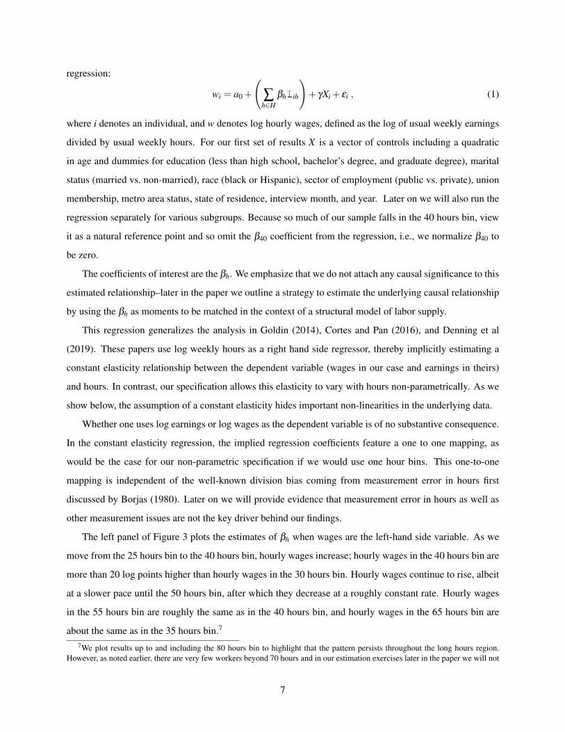
regression:

wi = a0 +

(∑

h∈Hβh1ih

)+ γXi + εi , (1)

where i denotes an individual, and w denotes log hourly wages, defined as the log of usual weekly earnings

divided by usual weekly hours. For our first set of results X is a vector of controls including a quadratic

in age and dummies for education (less than high school, bachelor’s degree, and graduate degree), marital

status (married vs. non-married), race (black or Hispanic), sector of employment (public vs. private), union

membership, metro area status, state of residence, interview month, and year. Later on we will also run the

regression separately for various subgroups. Because so much of our sample falls in the 40 hours bin, view

it as a natural reference point and so omit the β40 coefficient from the regression, i.e., we normalize β40 to

be zero.

The coefficients of interest are the βh. We emphasize that we do not attach any causal significance to this

estimated relationship–later in the paper we outline a strategy to estimate the underlying causal relationship

by using the βh as moments to be matched in the context of a structural model of labor supply.

This regression generalizes the analysis in Goldin (2014), Cortes and Pan (2016), and Denning et al

(2019). These papers use log weekly hours as a right hand side regressor, thereby implicitly estimating a

constant elasticity relationship between the dependent variable (wages in our case and earnings in theirs)

and hours. In contrast, our specification allows this elasticity to vary with hours non-parametrically. As we

show below, the assumption of a constant elasticity hides important non-linearities in the underlying data.

Whether one uses log earnings or log wages as the dependent variable is of no substantive consequence.

In the constant elasticity regression, the implied regression coefficients feature a one to one mapping, as

would be the case for our non-parametric specification if we would use one hour bins. This one-to-one

mapping is independent of the well-known division bias coming from measurement error in hours first

discussed by Borjas (1980). Later on we will provide evidence that measurement error in hours as well as

other measurement issues are not the key driver behind our findings.

The left panel of Figure 3 plots the estimates of βh when wages are the left-hand side variable. As we

move from the 25 hours bin to the 40 hours bin, hourly wages increase; hourly wages in the 40 hours bin are

more than 20 log points higher than hourly wages in the 30 hours bin. Hourly wages continue to rise, albeit

at a slower pace until the 50 hours bin, after which they decrease at a roughly constant rate. Hourly wages

in the 55 hours bin are roughly the same as in the 40 hours bin, and hourly wages in the 65 hours bin are

about the same as in the 35 hours bin.7

7We plot results up to and including the 80 hours bin to highlight that the pattern persists throughout the long hours region.However, as noted earlier, there are very few workers beyond 70 hours and in our estimation exercises later in the paper we will not

7

Figure 3: Cross-Sectional Relationship between Wages/Earnings and Hours

(a) log Hourly Wages-.5

-.4-.3

-.2-.1

0.1

log

of H

ourly

Wag

es

20 25 30 35 40 45 50 55 60 65 70 75 80Hours bin (usual weekly hours)

95% Confidence Interval

(b) log Weekly Earnings

-1-.8

-.6-.4

-.20

.2.4

.6lo

g of

Wee

kly

Earn

ings

20 25 30 35 40 45 50 55 60 65 70 75 80Hours bin (usual weekly hours)

95% Confidence Interval Earnings with constant wage

Figure 4: Cross-Sectional Relationship between Wages and Hours by Age and Education

(a) By Age

-.5-.4

-.3-.2

-.10

.1lo

g of

Hou

rly W

ages

20 25 30 35 40 45 50 55 60 65 70 75Hours bin (usual weekly hours)

25-34 35-44 45-54 55-64

(b) By Education-.5

-.4-.3

-.2-.1

0.1

log

of H

ourly

Wag

es

20 25 30 35 40 45 50 55 60 65 70 75Hours bin (usual weekly hours)

LHS HS Bach Bach+

The right panel of Figure 3 shows the results when we use usual weekly earnings as the left hand side

variable. The red line indicates how earnings at each level of hours would compare to the 40 hours bin if

there were a unitary elasticity, i.e., if wages were constant across the hours distribution. This figure clearly

shows why hourly wages decrease for hours above 50 in the left panel: earnings are close to flat above 50

hours.

Once again we are interested in how the relationship varies across age and education subgroups. While

our previous analysis allowed for age and education controls to shift wages, it did not allow them to interact

with the shape of the wage-hours profile. To pursue this possibility we repeat the analysis when splitting the

sample by age and education. Results are in Figure 4. Note that the Figure does not provide any information

put any weight on observations with 70 or more hours.

8

Figure 5: Cross-Sectional Relationship between Wages and Hours by Occupation (2010 Census MajorCategories)

-.8-.7

-.6-.5

-.4-.3

-.2-.1

0.1

.2lo

g of

Hou

rly W

ages

20 25 30 35 40 45 50 55 60 65 70 75 80Hours bin (usual weekly hours)

about wage differences across age or education groups since each curve shows wages relative to the 40 hours

bin for a given age or education, respectively. The left panel of Figure 4 presents the cross-sectional profile

of wages as a function of usual hours for each of several age groups, while the right panel does the same for

each of several educational attainment categories. The main message from this figure is that the same pattern

noted for the overall male population also holds for each age and education group. Some models of human

capital accumulation predict that young individuals work long hours at low wages because of the future

return to current hours. But significantly, Figure 4a shows that the cross-sectional patterns are effectively

the same for young and old workers. The overall shape of the wage-hours profile is also the same across all

education groups, but there is more hetereogeneity than by age. Although not shown, the main result also

holds when defining subgroups by both age and education.

We note that results for the wage-hours profile are essentially identical when splitting the sample by

any of the covariates used in our baseline regression, as well as others such as number of children, or even

spousal hours. And although our analysis in this paper focuses on males, it is of interest to note that we find

very similar results for females as well.

Although our subsequent analysis will not focus on occupational differences, it is also of interest to

explore this pattern within occupations. Figure 5 shows the results when we repeat the same exercise across

the census major occupation categories. While there is heterogeneity across occupations, the key point is

that for most occupations the slope of the wage-hours profiles is positive below 40 hours, and negative after

45 or 50 hours. Note that Figure 5 does not provide any information about occupational wage differences

since each curve shows wages relative to the 40 hours bin for a given occupation.

9

2.3.1 Variation Across Time and Data Sets

We mention two other exercises for which results are included in Appendix A. The first exercise concerns

the stability of the wage-hours profile over time. Fuentes and Leamer (2019) find that some quantitative

features of the earnings-hours profile have changed between the 1970s and the present. In particular, they

document that the additional earnings for working 50 rather than 40 hours has increased over this time

period. Appendix Figure A.1 shows that although the profile has changed between the 1970s and the present,

all of this change occurred prior to 1995; our estimated profile is very stable not only over the period 1995-

2007 but also when we extend the analysis to the present.8 Importantly, the fact that earnings flatten beyond

50 hours is a stable feature of the data over the entire post 1970 period. This is apparent in the figures in

Fuentes and Leamer (2019), and can also be seen in Appendix Figure A.1. That is, the decline in wages

beyond 50 hours is a robust feature of the data over the longer period covered by the data. Interestingly,

although Fuentes and Leamer (2019) present figures that clearly show the flattening of earnings beyond

50 hours, they do not highlight this feature of the data and so in particular do not draw attention to the

implication that wages decline beyond 50 hours.

The second exercise is to repeat our basic analysis using several other data sets: the CPS ASEC (i.e.

the March Supplement), the 2000 Census, the ACS, the PSID, and the NLSY79. While various details

vary across these data sets in terms of the basic measures that we utilize, Appendix Figure A.2 shows that

each of these generate not only the same qualitative shape for the wage-hours profile but also very similar

quantitative properties.

2.3.2 Wage vs Salary Workers

The previous analysis has shown that the hump-shaped wage-hours profile depicted in Figure 3 is robust to

controlling for a variety of observable characteristics. In this subsection we discuss one dimension along

which the pattern is not robust: the distinction of wage versus salaried workers. Figure 6 shows the wage-

hours profiles for each of these two groups. For reasons that we discuss shortly, and differently than before,

we normalize wages for both wage and salary workers relative to the earnings of salaried workers in the

40 hours bin. This Figure shows very different patterns when we stratify the sample by wage versus salary

worker. In particular, whereas the curve for salaried workers exhibits the same non-monotonic pattern that

we have previously emphasized, with the decrease starting at the 50 hours bin, the curve for wage workers

is effectively flat over the entire range above 40 hours, increasing modestly until 50 and then decreasing

8Similarly, Cha and Weeden document that the return to working 50 hours or more relative to working 35-49 hours has gone upbetween the 1970s and mid 1990s and has stabilized afterwards.

10

Figure 6: Cross-Sectional Relationship between Wages and Hours by Job-Type

-.6-.5

-.4-.3

-.2-.1

0.1

log

of W

eekl

y Ea

rnin

gs

20 25 30 35 40 45 50 55 60 65 70 75 80Hours bin (usual weekly hours)

Salaried Worker Hourly Wage Worker

Note: The shaded areas are the 95% confidence intervals.

modestly beyond 50. While these different patterns in the long hours region are striking, we argue that

they are of somewhat limited significance empirically. The first reason is that there are very few wage

workers who actually work long hours: whereas more than 30% of all salaried workers work long hours,

the comparable figure for wage workers is only about 10%. Equivalently, among workers who work long

hours, only one quarter of them are wage workers. Put somewhat differently, for workers who are assessing

their labor market opportunities conditional on working long hours, the vast majority of the opportunities

they would encounter would be salaried.

A second reason concerns the fact that wage workers have lower average wages than salaried workers

at 40 hours. Hence, even though the average wage worker who works 65 hours has wages that are roughly

the same as the average wage earner who works 40 hours, this individual earns basically the same average

wage as salaried workers who work 65 hours. One possible interpretation of the fact that wage workers have

a lower wage in the 40 hours bin is that their compensation package implicitly takes into account that they

will occasionally work more than 40 hours and receive overtime. To the extent that wage workers with hours

above 40 are receiving overtime pay, the constant average wage above 40 hours reflects a declining level of

base wages.

2.4 Other Cross-Sectional Patterns

The previously documented non-monotonicity in the cross-sectional wage-hours profile will play a central

role in our subsequent analysis. But once we go beyond characterizing the cross-sectional relationship be-

tween wages and hours by just first and second moments, it is of potential interest to also consider other

profiles. In this subsection we report three other profiles: the profile for mean hours across the wage dis-

11

Figure 7: More Moments by Education

(a) Mean log Wages-.7

-.6-.5

-.4-.3

-.2-.1

0.1

.2lo

g of

Hou

rly W

ages

20 25 30 35 40 45 50 55 60 65 70 75 80Hours bin (usual weekly hours)

LHS HS Bach Bach+

(b) S.D. log Wages

0.1

.2.3

.4.5

.6.7

.8.9

1S.

D. l

og o

f Hou

rly W

ages

20 25 30 35 40 45 50 55 60 65 70 75 80Hours bin (usual weekly hours)

LHS HS Bach Bach+

(c) Mean Hours

3032

3436

3840

4244

4648

50Av

erag

e H

ours

1 2 3 4 5 6 7 8 9 10Wage Decile

LHS HS Bach Bach+

(d) S.D. Hours

02

46

810

1214

1618

20Av

erag

e H

ours

1 2 3 4 5 6 7 8 9 10Wage Decile

LHS HS Bach Bach+

tribution, the profile for the standard deviation of log hourly wages across the usual hours distribution,

and the standard deviation of usual hours across the hourly wage distribution. When considering the wage

distribution we split the sample by deciles of the wage distribution.

For some of these moments one cannot run regressions with controls, but we can stratify the sample

by characteristics. Because our earlier analysis suggested large differences in the hours distribution by

education, we stratify by this variable and so plot all four cross-sectional profiles by education in Figure 7.

Panel (a) is simply a version of our earlier fact, but for consistency without any controls. It displays the same

pattern as in Figure 3 and Figure 4b. The remaining panels show the three additional cross-sectional profiles.

Both the mean and the standard deviation of hours are relatively constant across the wage distribution for

all education groups, with the lone exception of the very lowest wage decile. The standard deviation of log

wages exhibits a modest increasing pattern for hours above 40 for all education groups. Below 40 hours the

12

patterns differ somewhat between the lower and higher education groups.

While we will not explicitly use these moments in our estimation exercise, we will assess the model’s fit

along these dimensions.

2.5 Measurement Issues

One of the striking patterns that we documented in the preceding subsections is that in the cross-section

wages tend to fall with usual hours worked beyond 50 hours, reflecting the fact that earnings were relatively

flat beyond 50 hours. One concern is that this decline in wages may be an artifact of measurement issues.

In this subsection we summarize the results from several robustness checks and conclude that the decline in

wages above 50 hours is not solely the result of measurement issues. More details can be found in Appendix

B.

The first possibility we consider is that the comparatively flat earnings coefficients above 50 hours shown

in Figure 3b are driven by top-coding. Top coding is of very minor importance for those with usual weekly

hours below 45 hours, but does increase in importance with the level of usual weekly hours, increasing

from just under 6 percent for those in the 50− 54 hours bin to about 10 percent for those in the 60− 64

and 65− 69 hours bins. Nonetheless, we argue in Appendix B that top-coding does not appear to be of

first order importance. For those with graduate degrees the incidence of top-coding is more substantial

and it appears that top-coding can potentially shift the estimated wage-hours profile somewhat, and hence

modestly dampen the rate at which wages decrease in the long hours region.

A second possibility is that individuals in the long hours region are salaried workers who face temporary

variation in hours but have a fixed salary. In this sense, salary reflects expected hours rather than actual hours.

If long hours individuals are disproportionately those with temporarily high hours, this would tend to flatten

the earnings profile.9 We assess this explanation using the small panel component of the CPS ORG to create

a sample in which we have two observations per individual. If we average across the two observations we

should dampen the effect of temporary variation in usual hours in the face of fixed compensation. However,

when we run this alternative specification we find the same pattern quantitatively. We have also pursued

this using the NLSY79, which allows us to average over more years. Our main finding remains when we

average over a five year period.

The third and related possibility that we consider is measurement error in hours. If people with high

hours tend to be people who have over-reported their hours then this will show up as a negative effect of

hours on wages. Our structural analysis later in the paper will incorporate measurement error in hours, so

9Denning et al (2019) suggest that this explanation accounts for the low elasticity of wages to hours when using actual hours.

13

our inference will take this into account. But here we note that if classical measurement error was driving the

results then we would expect the averaging exercise just described above to produce very different patterns,

which it does not.

The previous exercise does not rule out some measurement error stories that rely on non-classical mea-

surement error. For example, perhaps many long hours individuals tend to over-report hours. To assess this

we use the linked observations between the CPS ORG and the American Time Use Survey (ATUS) from

IPUMS, see Hofferth et al (2018), which feature information on usual weekly hours with a single observa-

tion on hours actually worked for a particular day. By pooling across individuals we can compute a synthetic

measure of average weekly hours from the ATUS for individuals with reported usual hours in the CPS ORG

within a particular hours bin.

Detailed results from this exercise are presented in Appendix C. Here we summarize the key findings.

First, we find that the two values track each other very closely up to usual hours below 70.10 Second, while

our measure of synthetic weekly hours computed from the ATUS is systematically lower than the reported

measure in the CPS ORG and the gap grows as hours increase above 40, the difference remains relatively

small, reaching around 5 hours per week in the 65-69 hours bin. In percentage terms, the gap is relatively

constant in the 50-69 hours range, staying in the range of 6.5% to 8.5%.

While not insignificant, this discrepancy has little potential to change our key finding of flat earnings

and decreasing wages above 50 hours. The reason is simple: if earnings are flat beyond 50 hours, then

moving individuals from higher to lower hours bins does not affect earnings within a bin and hence will not

affect average wages within a bin. Similarly, if hours are systematically overstated by a relatively constant

percentage above 50, this will cause a uniform decrease in measured wages relative to true wages, and so

will not affect the slope of the wage-hours profile above 50 hours.

In Appendix C we report results from an exercise in which we adjust CPS hours based on the gap with

reported hours in the ATUS and then repeat our exercises. The key message is that this adjustment has

virtually no effect on the behavior of wages and hours beyond 50 hours. In summary, taking reported hours

from the ATUS time diaries at face value, our analysis of linked CPS ORG-ATUS data leads us to conclude

that systematic over-reporting of usual weekly hours is not the dominant explanation for the relatively flat

earnings beyond 50 hours.

Lastly, we have used the long panel feature of the NLSY to further cast doubt on the possibility that

reported hours above 50 largely represent measurement error. As noted earlier, using the cross-section

10There are very few individuals with usual hours of 70 or more and as noted earlier, we will not use these observations in ouranalysis later in the paper. For this reason we do not devote any attention to the larger discrepancy from 70 hours onwards.

14

component of the NLSY we get essentially the same results that we found in the CPS ORG. We then use

the panel component of the NLSY and find that individuals with high reported hours tend to have higher

future wage growth, consistent with the evidence presented in Imai and Keane (2004) and Michelacci and

Pijoan-Mas (2012).11 If long hours were simply the result of individuals over-reporting their hours in a

persistent fashion then we would not expect to see that high hours are predictive of future wage growth.

In summary, while we think that measurement error plays some role in shaping the observed profile of

mean wages versus usual weekly hours, and will include it in our later analysis, we do not think that the rel-

atively flat earnings in the long hours region and the resulting decline in wage rates is purely a measurement

artifact.

3 A Structural Model of Hours and Wages in the Cross-Section

In this section we develop a static model of labor supply featuring workers that are heterogeneous in pro-

ductivity and tastes for work and show that it can account for the cross-sectional patterns that we have

documented. The key novel feature of the model is that earnings are a non-linear function of hours and the

nature of this non-linearity varies over the hours distribution. Because our model is static, we estimate it

using data on workers aged 50-54, for whom dynamic considerations such as human capital accumulation

are likely to be less important. We view this as an important first step to developing a richer analysis that

also includes dynamic effects and includes data for younger workers.

3.1 A Linear Earnings Benchmark

We begin by analyzing a benchmark model in which earnings are linear in hours. This static model closely

resembles the labor supply problem in the model of Heathcote et al (2014). We show that while it can

account for the covariance between log hours and log wages in the cross-section, it is not able to account for

the key features documented in Sections 2.2-2.3. This will motivate the extension to non-linear earnings.

There is a unit mass of individuals with preferences over consumption and hours of work given by:

11− (1/σ)

c1− 1

σ

i − αi

1+(1/γ)h

1+ 1γ

i

Individuals are heterogeneous in terms of preferences for work, captured by the parameter αi, and produc-

tivity, which is denoted by zi. The two preference parameters σ and γ are the same for all individuals.

11See aslo Gicheva (2013) and Barlevy and Neal (2019) for evidence on dynamic effects in the context of professional labormarkets.

15

Table 1: Calibration of Linear Earnings Model

Data Moment Model Parametermean(logh) = 3.740 µα =−11.228mean(logw) = 2.804 µz = 0

std(logh) = 0.122 σα = 0.369std(logw) = 0.460 σz = 0.468

corr(logw, logh) = 0.067 ρzα =−0.064

We assume that α and z are jointly log normally distributed. This joint distribution is characterized by

five values: the mean and standard deviation of logz, the mean and standard deviation of logα , and the

correlation between logz and logα , which we denote by µz, σz, µα , σα , and ρzα respectively.

All individuals face a wage per efficiency unit equal to w, so that normalizing the price of consumption

to unity the budget equation for individual i is given by:

ci = wzihi.

At this point we abstract from taxes, though we include them later on in a sensitivity exercise. As a practical

matter the value of w can be subsumed into the mean of zi and so in what follows we will normalize it to

unity. Importantly, the budget equation that a given individual faces is linear in hours.

Each individual maximizes their utility subject to this budget equation. The optimal choice of hours for

an individual with idiosyncratic values αi and zi is given by:

loghi =1

(1/σ +1/γ)

(σ −1

σlogzi + logαi

)Given values for σ and γ , and values for the mean of log hours, the mean of log wages and the covariance

matrix between log hours and log wages, there is a unique set of the five distributional parameters that can

match these five values. For now we abstract from measurement error, as it does not impact the main

message of this exercise, but we will introduce it in the next subsection when we extend this model. Table

1 displays the values of these five moments from the data are given in the first column of Table 1, and the

second column shows the implied values for the model parameters for the case in which σ = 1 and γ = .50.12

While this linear earnings model can account for some basic properties of the cross-sectional distribution

of hours and wages, it is unable to account for the key features of the hours distribution and the wage-hours

12As noted previously, the values of the five moments differ based on gender, age and education. The values reported herecorrespond to the subsample of males aged 50-54 with a high school education with usual hours worked between 30 and 70. Wechoose this subsample here because it is the subsample we will use for our main exercise later on. Reasons for choosing thissubsample are explained later.

16

Figure 8: Fit of Linear Earnings Model

(a) Wage-Hours Profile

30 35 40 45 50 55 60 65Usual Weekly Hours

0.6

0.4

0.2

0.0

0.2

0.4DataModel

(b) Share of Workers by 5-Hour Bins

30 40 50 60Usual Weekly Hours

0.0

0.1

0.2

0.3

0.4

0.5

0.6

0.7 DataModel

profile documented in Sections 2.2-2.3. Figure 8 shows the model predictions versus their counterparts in

the data for our sample. Two key issues stand out. First, the model fails to generate the heavy concentration

of individuals in the 40 hours bin, has too many individuals working part-time, and not enough individuals

working long hours. Second, wages are monotonic across the hours distribution, exhibiting a mild upward

slope.

Adding classical measurement error in hours and assuming that hourly wages are computed as the ratio

of earnings to hours would induce a negative slope to the wage-hours profile, but importantly would still not

generate the non-monotonicity found in the data. If measurement error were present, the negative correlation

between hours and wages that it induces would be undone in the calibration procedure by the choice of ρzα

so as to still yield the target level for this correlation. Similarly, deviating from σ = 1 (i.e., not imposing

that income and substitution effects are offsetting) would affect this correlation holding all else constant, but

this effect would again be undone by the calibration of ρzα .

It is important to note the significant role that parametric assumptions on the distribution of individual

heterogeneity play in these findings. Absent such restrictions, the linear earnings model with two dimensions

of heterogeneity at the individual level can perfectly account for any cross-sectional pattern of hours and

wages. To see why, note that we could use the wage data to pin down the individual values of the zi and then

use the hours data to pin down the individual values of the αi. This second step can be done for any values

of σ and γ .

Importantly, this non-parametric analysis places no restrictions on the joint distribution of the zi and the

αi. This motivates us to examine what the implied joint distribution of z and α would look like if we used

the data on hours and earnings to infer the distribution non-parametrically. Here we briefly summarize two

17

results.

First, with σ = 1, matching the concentration of workers in the 40 hours bin requires a spike in the

distribution of α . If σ is not equal to unity, there must be a spike in the conditional density for α for each

value of z, and the position of this spike varies systematically with the value of z. To us this seems a very

unappealing assumption. Second, matching the non-monotonicity in the relation between wages and hours

requires that the correlation between α and z changes sign across the hours distribution. We think that this

is also an unappealing assumption.

These implications suggest that it is of interest to explore specifications in which we can account for

the cross-sectional patterns when imposing more standard distributional assumptions. With this in mind, we

will continue to assume that the zi and αi are jointly log normally distributed going forward.

3.2 Nonlinear Earnings

Normalizing the wage per efficiency unit of labor to unity as above, we generalize the previous model along

one dimension by assuming that individuals face a nonlinear schedule for earnings as a function of hours,

so that the budget equation for individual i is now given by:

ci = ziA(hi)hθ(hi)i = ziE(hi)

We assume that the function E(h) is continuous in h but do not require that θ(h) is continuous. We include

the A(h) term as a way to maintain continuity of the earnings function at a point of discontinuity in the

θ(h) function. That is, the function A(h) is constant in any interval in which θ(h) is continuous, and as a

normalization we impose A(0) = 1. The appeal of this functional form is that the function θ(h) provides a

clear and flexible mapping from hours into the marginal effect of hours on earnings. In what follows we will

refer to E(h) as the earnings function. We also define the wage function, W (h), defined by:

W (h) =E(h)

h= A(h)hθ(h)−1

which gives the average earnings per hour for an individual with zi = 1 who works h hours. Our specification

generalizes the one first used by French (2005) in which θ(h) was constant.

It is intuitive that this extension might help to account for the properties of the cross-sectional distribution

of hours and wages that the linear earnings model could not explain. First, non-linearities in the earnings

function will necessarily impact the shape of the wage profile across the hours distribution. Second, a kink

in the earnings function associated with a downward jump in θ(h) will tend to generate bunching in the

18

hours worked distribution. In what follows our goal is to assess the extent to which this extension helps us

to account for the patterns in the data, and if so, what it implies for the shape of the θ(h) function.

3.3 Measurement Error

As noted in Section 2.5, measurement error in hours is potentially important because it induces a negative

correlation between measured hours and measured wages when wages are derived as the ratio of earnings to

hours. Although we previously argued that the non-monotonic wage-hours profile is not purely a reflection

of measurement error, we do want to allow for the possibility that measurement error plays some role.

In our benchmark exercise we allow for measurement error in log hours that is classical subject to one

qualification. The qualification is that if an individual has true hours equal to 40 we assume that they do not

report with measurement error. The rationale for this is intuitive–it is virtually impossible to generate a large

spike at 40 hours if we assume that everyone reports hours with classical measurement error. In fact, there

is good reason to believe that measurement error more likely serves to increase the spike at 40 rather than

diminish it, since another feature of the reported usual hours distribution is that there is heaping at all values

ending in either a zero or a five. A natural interpretation is that individuals tend to round to a multiple of

five when reporting usual weekly hours. We do not attempt to incorporate this type of measurement error,

but this partly motivates our decision to focus on hours bins when we connect our model to the data.

For those who do not work exactly 40 hours we assume that log hours are reported with normally

distributed measurement error that is iid across individuals with mean zero and standard deviation σm. In

contrast to measurement error in hours, classical measurement error in log earnings has relatively little

impact on our findings. Within an hours bin, this type of measurement error has no impact on the average

log earnings in the bin and little impact on average log wages. Classical measurement error in earnings does

impact the overall correlation between wages and hours, but for reasonable values of measurement error this

effect is small. For this reason we abstract from measurement error in earnings in what follows.13

3.4 Moment Matching Exercise

We now describe our main quantitative exercise. The goal is to choose values for our model parameters

so that the model matches a large set of key empirical moments for hours worked and wages. The result-

ing parameterized model will generate a relationship between hours and wages that reflects a combination

of heterogeneity across workers, measurement error, and the causal effect of hours on wages. From this

13Heathcote et al (2014) estimated no measurement error in earnings, which they argued was consistent with other results in theliterature.

19

exercise we can infer both the extent to which the observed cross-sectional moments reflect selection of

heterogeneous individuals and the extent to which hours of work influence wages.

We emphasize that our approach is focused on understanding the patterns in the data from a pure labor

supply perspective. That is, we assume that each individual is free to choose their hours of work, taking as

given the trade-off in terms of hours and wages reflected by the wage function W (h). We thus abstract from

the possibility that an individual who works 40 hours did not have the option to work a different number of

hours. Instead, we assume that the wages being offered for other levels of hours were such that the individual

preferred to work 40 hours. To the extent that firms do not desire to hire workers for a particular level of

hours, this will manifest itself by having low wages associated with that level of hours. That is, our earnings

function embeds factors that operate on the firm side and affect the demand for different workweeks. We

emphasize that our earnings function should be interpreted as the opportunities that the worker faces in the

market more broadly and not necessarily the options available at a given firm. We also abstract from any

search frictions a worker might face in finding a job with a particular bundle of hours and wages.14

The choice of a functional form for θ(h) in our benchmark specification reflects a minimal departure

from the specification previously used by French (2005) and others. In particular, rather than assuming

that θ(h) is constant, we instead assume that θ(h) is a step function, assuming one value θs for h below

40, and a different value θl for h greater than or equal to 40. The choice of 40 hours for the position of

the step is empirically motivated, since workers will tend to concentrate their hours at a kink in the earnings

function. This specification has the appealing feature of allowing different hours-wage trade-offs for workers

desiring part-time work schedules and workers desiring longer work schedules. While our specification of

θ(h) imposes quite a bit of structure we will see that it is sufficiently flexible to account quite well for the

features of the data that we target.15 As discussed later, we found that several generalizations did not have a

significant impact on the results.

Our specification for θ(h) implies that all individuals will work positive hours, so there is no selection

of individuals into employment. Introducing fixed costs as in Cogan (1981) or altering the shape of the

earnings function at low hours as in Prescott et al (2009) would allow us to generate an active extensive

margin. Given our application to male workers we do not believe this is a first order issue and so do not

pursue it in this paper.

In all cases we fix the values of σ and γ . Our exercise can be implemented for any values of these

14Altonji and Paxson (1988) emphasized workers seeking to change their usual weekly hours as a source of turnover at the firmlevel.

15The wage profile actually suggests that one might want to include a separate region for hours below 30. It would be relativelysimple to do this. But given that our current application is based on data for males and there are so few males in that region, wehave chosen to not focus on that region and reduce the set of parameters.

20

parameters, but in what follows our benchmark results consider the case in which σ tends to one, implying

offsetting income and substitution effects, and γ = 0.50. We discuss later how alternative choices for σ

would affect our findings. The value of γ is not important for our exercise because changes in γ will be

undone by changes in the standard deviation of the preference shocks.

Our choices up to this point leave seven parameters whose values are not yet assigned: the four parame-

ters for the joint distribution of z and α (µα , σα , σz, and ραz, recalling that we normalized µz to equal 0), the

two θ j values that define the earnings function and σm, the standard deviation of classical measurement error

in log hours. Our moment matching exercise is a natural extension of the moment matching exercise used

to calibrate the parameters of the simple model. In that case we matched the mean of the hours distribution,

the standard deviation of log hours, the standard deviation of log wages and the correlation between log

hours and log wages. We showed that although the model could perfectly replicate these moments, it could

not account for salient features of the hours distribution and the empirical wage-hours profile. We now in-

clude these additional moments in our moment matching exercise. Specifically, we include the distribution

of workers across ten hour bins between 30 and 70, and the empirical wage profile across five hour bins

between 30 and 70.16,17 Because we are adding moments of the hours distribution we do not include the

mean and standard deviation of log hours as explicit moments. We choose parameter values that minimize

the sum of squared deviations from the target moments.

Before proceeding to the results we provide some heuristic discussion to indicate how both the hours

distribution and the wage profile play a role in shaping the identification of the model parameters. In our

benchmark specification with σ = 1, the choice of hours is independent of z and as a result the hours

distribution depends only on the four parameters µα , σα , θs and θl . Our estimation procedure has four

targets relating to the hours distribution (the share of workers in each of the four ten hours bins between

30 and 69) and so one could think of these four parameters as being determined by the hours distribution.

Importantly, this procedure would estimate the values of θs and θl without using any data on wages. With

θs and θl fixed, the issue of matching the wage-hours profile effectively becomes one of generating an

appropriate pattern of selection, since the difference between the wage function E(h)/h and the wage-hours

profile reflects how worker productivity varies across hours bins.

However, if µα , σα , θs and θl are targeted using only data on the hours distribution, there are only

16We use the share of workers in ten hour bins instead of five hours bins for reasons related to our earlier discussion of measure-ment error. Specifically, the data suggests that there is more heaping at multiples of ten rather than at the intermediate values. With5 hour bins and only classical measurement error our model will not be able to account for this feature.

17For our current sample of males aged 50−54 only 3 percent of the observations lie outside of the 30−70 hours range, which iswhy we do not seek to include wages for those workers in the moment matching exercise. As noted earlier, if we wanted to matchwages for those with hours below 30 we would need to include a third region for the step function θ(h).

21

two remaining parameters, σz and ρzα , that can be varied to affect the selection of workers across hours

bins. These two parameters clearly have a direct effect on selection, but selection is also influenced by the

other four parameters. Intuitively, if z and α are correlated and we know the distribution of α then this has

implications for the distribution of z, thus explaining why σα will influence selection. But equally important,

the values of θs and θl influence the amount of selection needed to fit the wage-hours profile, so changing

these values can affect the ability of the model to generate the amount of selection that is needed.

It thus turns out that there is a tradeoff between matching the hours distribution and the wage-hours

profile; i.e., the values of µα , σα , θs and θl are also influenced by the wage-hours profile. Our estimated

parameters are chosen to balance the tradeoff between matching the hours distribution and the wage-hours

profile using our loss function.

4 Results

The procedure that we describe above could be applied to data for any subsample. In this section we report

the results from implementing it on a sample of males aged 50−54 with a high school education (including

some college). A few issues motivate our choice of this particular subsample. One reason for focusing on

a sample of males rather than females at this point is that we have abstracted away from the participation

margin, and this margin is arguably less important for a male sample. Our choice of age group balances the

desire to have an age group for which extensive margin considerations due to early retirement are not too

important at the same time that the potential dynamic returns to working additional hours are less relevant. It

is common in the human capital literature to assume that individuals in the 50−54 age group face very low

returns to additional human capital accumulation, see for example, Heckman et al (1998). We stratify by

education since it is plausible that earnings functions may vary with education. We have also implemented

our exercise on the sample of males aged 50− 54 with at least a college education and found very similar

results, both in terms of implied values for the θ j and the fit of the model, so in the interests of space we

focus on the results for the high school sample.

We note that the distribution of worker level characteristics α and z in this exercise should be interpreted

as potentially reflecting any history dependent evolutions. In particular, our specification is fully consistent

with the possibility that choices about hours of work when young had effects on both future productivity

and tastes for work when old. What we assume is that for individuals aged 50-54 these dynamic effects are

no longer relevant.

Table 2 displays the parameter values generated from our moment matching exercise.

22

Table 2: Estimated Parameter Value

µα σα σz ρα,z θs θl σm

−12.936 1.127 0.510 −0.375 1.40 0.11 0.04

Table 3: Fit of Estimated Model

Data Modelmean (logh) 3.744 3.744mean (logw) 2.804 2.804

std (logh) 0.122 0.126std (logw) 0.460 0.460

corr (logh, logw) 0.067 0.067

4.1 First and Second Moments for Hours and Wages

As a first step in evaluating the model’s ability to fit the moments of interest from the data, Table 3 shows

that the estimated model also does an excellent job in matching the moments that the simple linear earnings

model was able to perfectly replicate.

4.2 The Wage-Hours Profile

Next we examine how well our model accounts for the properties that the linear earnings model could not

account for. We begin with the wage-hours profile. The left panel of Figure 9 shows that the profile in the

estimated model does a good job of tracking the empirical profile, though its peak occurs a bit before the

peak in the data. The profile generated by the model reflects both the sorting of individuals across the hours

profile, the non-linearities of the wage function and measurement error. One of our goals is to ascertain

the quantitative significance of each component. To pursue this, the right panel of Figure 9 plots the model

generated wage-hours profile, the model generated wage-hours profile assuming no measurement error, the

wage function (i.e., E(h)/h) and the mean value of productivity z across the hours bins. The figure shows

that measurement error does not play a large role in shaping the model generated wage-hours profile.18 The

hump-shaped pattern for the wage function reflects the estimated values of the two θ j parameters. Recalling

that a value of θ j > 1 implies that hourly wages are increasing in the number of hours worked, θs = 1.40

18There is no definitive value for the extent of measurement error in hours. Assuming that measurement error is classical andiid over time then transitory variation in hours provides some information about plausible values. Our estimate of σm = 0.04 issomewhat small relative to the estimates in Heathcote et al (2014) regarding the variance of the transitory component of hours. Butnot all transitory variation in hours need be measurement error. Duncan and Hill (1985) and Bound et al (1994) are two examplesof small scale studies documenting discrepancy between adminsitrative data and survey responses. They find even larger estimatesof measurement error in hours. But administrative data may provide a poor measure of usual hours for salaried workers. See alsothe survey article by Bound et al (2001).

23

Figure 9: The Wage-Hours Profile in our Benchmark Estimation

(a) Fit of Wage-Hours Profile to Data

30 35 40 45 50 55 60 65Usual Weekly Hours

0.6

0.4

0.2

0.0

0.2

0.4DataModel

(b) Determinants of the Wage-Hours Profile

30 35 40 45 50 55 60 65Usual Weekly Hours

0.6

0.4

0.2

0.0

0.2

0.4

Mean WagesMean Wages, no m.e.Wage FunctionMean Productivity

implies a substantial wage gain associated with moving from part-time to full time work. The value of

θl = 0.10 is not only much lower than θs but is also much less than unity, implying that although earnings

continue to increase, wages per hour worked actually decrease as hours increase beyond 40 hours.

The gaps between the wage function and the wage-hours profile reflect the role of selection. Note that

these gaps are of different sign on either side of the 40 hour bin. This reflects that our estimated value of

ρzα is −0.375, indicating that individuals with low disutility for working tend to be more productive. To

see why, note that our benchmark specification with σ = 1 implies that hours of work are independent of z,

depending solely on α . It follows that if z and α were uncorrelated and there were no measurement error,

the wage-hours profile generated by the model would be identical to the wage function. However, a negative

value for ρzα implies that high hours individuals tend to have higher productivity, and low hours individuals

tend to have lower productivity, thereby explaining why the gaps are of different signs on either side of the

40 hours bin.

The size of the selection effects are large. For example, the wage penalty associated with working 30

rather than 40 hours is roughly eleven percent, whereas the cross-sectional wage-hours profile indicates that

average wages for individuals in the 30 hours bin are more than 40 percent lower than those in the 40 hours

bin. We note that our estimated penalty for part-time work is similar to the estimates in Aaronson and French

(2004) that leveraged features of Social Security to isolate plausibly exogenous movements from full-time

work to part-time work.

We summarize by noting four implications from our estimated model. First, there is a large kink in

the earnings function at h = 40. Second, there is a significant part-time wage penalty. Third, the ability

individuals to generate higher current earnings by working hours beyond 40 is very limited compared to

24

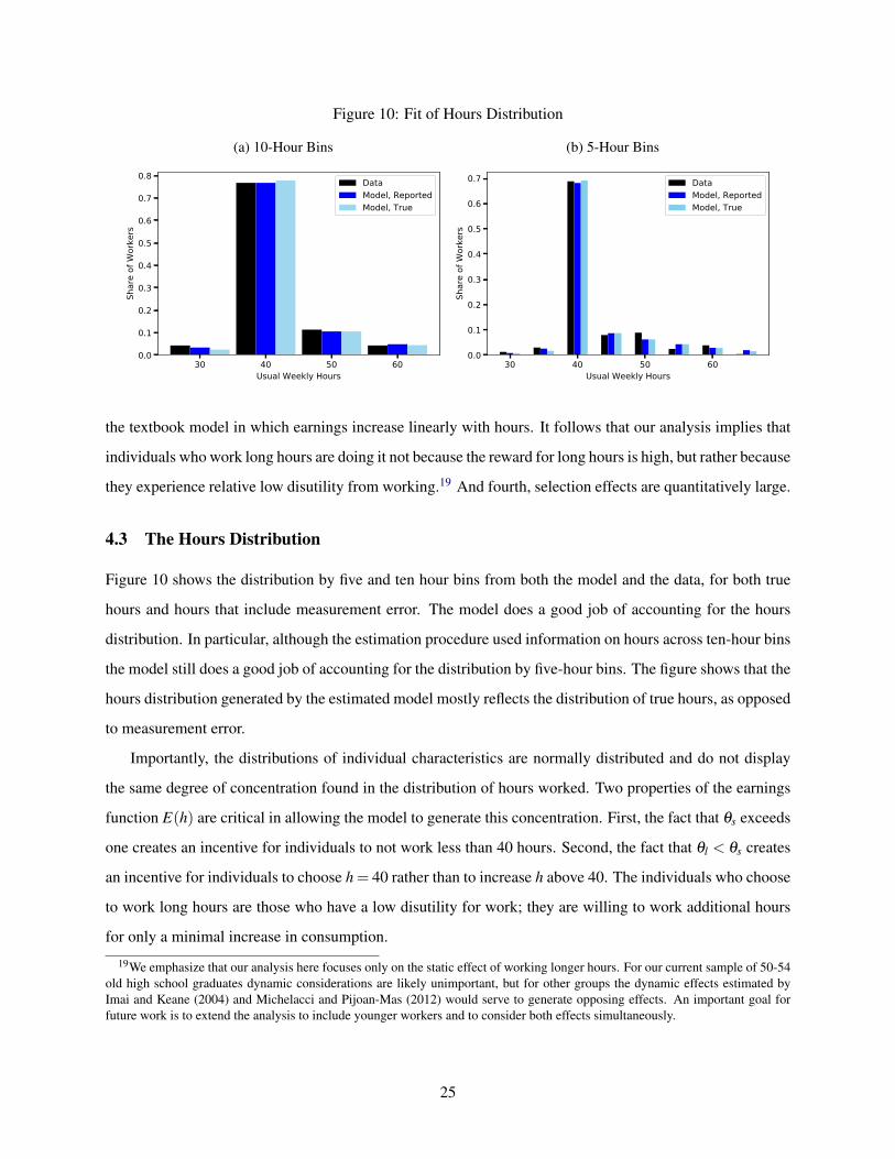
Figure 10: Fit of Hours Distribution

(a) 10-Hour Bins

30 40 50 60Usual Weekly Hours

0.0

0.1

0.2

0.3

0.4

0.5

0.6

0.7

0.8

Shar

e of

Wor

kers

DataModel, ReportedModel, True

(b) 5-Hour Bins

30 40 50 60Usual Weekly Hours

0.0

0.1

0.2

0.3

0.4

0.5

0.6

0.7

Shar

e of

Wor

kers

DataModel, ReportedModel, True

the textbook model in which earnings increase linearly with hours. It follows that our analysis implies that

individuals who work long hours are doing it not because the reward for long hours is high, but rather because

they experience relative low disutility from working.19 And fourth, selection effects are quantitatively large.

4.3 The Hours Distribution

Figure 10 shows the distribution by five and ten hour bins from both the model and the data, for both true

hours and hours that include measurement error. The model does a good job of accounting for the hours

distribution. In particular, although the estimation procedure used information on hours across ten-hour bins

the model still does a good job of accounting for the distribution by five-hour bins. The figure shows that the

hours distribution generated by the estimated model mostly reflects the distribution of true hours, as opposed

to measurement error.

Importantly, the distributions of individual characteristics are normally distributed and do not display

the same degree of concentration found in the distribution of hours worked. Two properties of the earnings

function E(h) are critical in allowing the model to generate this concentration. First, the fact that θs exceeds

one creates an incentive for individuals to not work less than 40 hours. Second, the fact that θl < θs creates

an incentive for individuals to choose h = 40 rather than to increase h above 40. The individuals who choose

to work long hours are those who have a low disutility for work; they are willing to work additional hours

for only a minimal increase in consumption.

19We emphasize that our analysis here focuses only on the static effect of working longer hours. For our current sample of 50-54old high school graduates dynamic considerations are likely unimportant, but for other groups the dynamic effects estimated byImai and Keane (2004) and Michelacci and Pijoan-Mas (2012) would serve to generate opposing effects. An important goal forfuture work is to extend the analysis to include younger workers and to consider both effects simultaneously.

25

Figure 11: Fit of Other Wage and Hour Profiles

(a) Mean log Wages

30 35 40 45 50 55 60 65Usual Weekly Hours

0.6

0.4

0.2

0.0

0.2

0.4DataModel

(b) S.D. log Wages

30 35 40 45 50 55 60 65Usual Weekly Hours

0.0

0.1

0.2

0.3

0.4

0.5

0.6

0.7

SD lo

g W

ages

DataModel

(c) Mean Hours

2 4 6 8 10Wage Decile

34

36

38

40

42

44

46

48

50

Mea

n Ho

urs

DataModel

(d) S.D. Hours

2 4 6 8 10Wage Decile

0

2

4

6

8

10

12

14SD

log

Hour

sDataModel

4.4 Other Profiles

In Section 2 we presented evidence on three other profiles: the standard deviation of wages across the hours

distribution, and the mean and standard deviation of hours across the wage distribution. We did not use these

moments in our estimation exercise but here we report on how well the estimated model fits the empirical

moments. Results are in Figure 11. The model profile for the standard deviation of hours across the wage

distribution is relatively flat in both the data and the model, but the level is uniformly higher in the model

than in the data, suggesting that we have a bit too much hours variation within each wage cell. But overall

we feel that the model does a good job of replicating these profiles despite the fact that they were not targeted

as part of the estimation.

26

4.5 Interpreting the Kink in the Earnings Function

Having estimated a sharply kinked earnings function we think it is important to have some discussion on

how we interpret this function. We think that our earnings function reflects two distinct but related forces.

The first force reflects the extent to which average labor services (or efficiency units) per hour are affected

by the length of the workweek. For example, if there are some set-up costs involved, then labor services

may be convex in hours at low levels of hours, and if individuals become fatigued at long hours then there

may be a concave region at higher levels of hours. Barzel (1973) and Rosen (1978) both emphasized this

source of nonlinearities. See Pencavel (2015) for a discussion of this issue and evidence in one particular

setting.

The second force reflects coordination. The issue of coordination exists both within and across produc-

tion units. The assembly line is the classic example of a production process that requires workers within

a given business to coordinate their work schedules. But more generally, any business that has frequent

interactions with other businesses has a desire to coordinate work hours with other businesses. The need to

coordinate will necessarily lead to firms placing different value on workweeks of different lengths. Yurdagul

(2017) posits an aggregate production function in which inputs of different workers are complements, im-

plying that workweeks for a particular worker are less valued as they move further from mean hours across

other workers.

We view our estimated earnings function as reflecting both of these forces and we do not attempt to

separately identify them. To the extent that the kink at 40 hours reflects coordination, we do not think there

is necessarily anything fundamental about the position of the kink that we estimate. In a different setting

the kink may well happen at a different level. Alternatively, if the kink reflects set-up costs and fatigue, then

a kink in the area around 40 hours might be viewed as something fundamental to the technology of effort

provision, though of course this technology might vary across different tasks or occupations. Finally, the

two channels could be complementary in the sense that a moderate increase in fatigue beginning around 40

hours might induce coordination around that point, exacerbating the kink in the earnings technology.

4.6 Sensitivity

In this subsection we consider four sensitivity exercises: alternative values of σ , progressive taxation, alter-

native specifications for E(h), and fat tailed distributions.

27

4.6.1 Alternative Values of σ

Our benchmark specification had σ = 1, implying offsetting income and substitution effects. One might

conjecture that this would play a significant role, since deviating from this case would necessarily influence

the cross-sectional correlation between hours and wages. However, considering empirically plausible alter-

native values for σ has virtually no impact on our estimated earnings function. The reason is the same as

mentioned in our estimation of the linear earnings model: as we vary σ the estimated value of ρzα changes

so as to basically offset the cross-sectional correlation between hours and wages that is induced by σ . The

net effect is that the estimated values of θs and θl barely change.

Loosely speaking, when income effects dominate substitution effects (which is the more interesting case

empirically), low productivity individuals tend to work longer hours, leading to negative selection of high

hours individuals on productivity. But this selection effect can be undone by changes in ρzα , and this is what

happens in our estimation.

4.6.2 Progressive Taxation

Our benchmark model abstracts from taxes when estimating the non-linearities in the earnings function.

Because progressive taxes generate non-linearities between hours and after-tax income it is of interest to

examine how including them affects our estimates. We adopt the specification from Heathcote et al (2014)

in which the average tax rate facing an individual is given by:

τ(y) = 1− τ0y−τ1

where y is an individual’s income relative to mean income, τ1 determines the extent of progressivity and

τ0 is a constant that influences the overall average tax rate. Simple algebra shows that this generates the

following budget equation:

c = τ0y1−τ1

where τ0 is a constant depending on mean income and τ0.20 The value of τ0 is irrelevant for our exercise

as its impact will be undone by the calibration of mean tastes for work. The literature suggests a range of

empirically plausible estimates for τ1; Guner et al (2014) estimate τ1 = 0.060 using IRS tax returns while

Heathcote et al (2014) estimate τ1 = 0.185 using NBER TAXsim for their sample of CPS households.

We have repeated our estimation exercise with this extension for each of the two values of τ1 reported

20We note that Benabou (2002) simply started with this expression to capture a progressive tax system.

28

above. In both cases the impact on the results is minimal.

To see why progressive taxation has only a minor impact on our estimates, first note that progressive

taxes have no direct effect on targeted wage moments, which are pre-tax. But they do potentially have a

direct effect on the choice of hours. To assess this, we focus on the σ = 1 case which implies the following

first order condition for h for any individual away from the kink:

logh =logθ j + log(1− τ1)− log(α)

1+(1/γ)

where θ j corresponds to the relevant region. It follows that by adjusting the mean of logα one can com-

pletely offset the effect of progressive taxes in this expression. However, even with this adjustment, progres-

sive taxes will affect the choice of individuals to locate at the kink since increasing h above 40 becomes less

attractive at the margin. But as a practical matter this effect is relatively small so that there is little change

in estimated parameters beyond the change in the mean of logα .

4.6.3 Alternative Specification for E(h)

Our benchmark model imposed that E(h) was a step function with two values. It is of interest to gauge the

extent to which other specifications might affect our results.

We note that imposing a kink at 40 is essentially dictated by the data; absent a kink at this position there

is no way to both get a significant mass of workers working long hours and the concentration around 40

hours. For this reason we do not consider departures from this feature. We originally tried a specification

that allows for steps at both 40 and 50 hours, motivated by the shape of the wage-hours profile. But we

found that the two elasticities were very similar, leading us to assume a single elasticity in the over 40 hours

region.

More generally, we also considered the following smooth alternative for the variation of θ above 40:

θ(h) = a+bθ for h≥ 40

where we now estimate the two parameters a and b. Perhaps not too surprisingly given the previous result,

we find that this specification yields a very similar fit to the data and that the parameter b is estimated to be

very close to zero.

29

4.6.4 Fat Tailed Distributions

We previously commented on the role of parametric assumptions on heterogeneity. Assuming log-normality

we found that the linear earnings model could not generate a large concentration around 40 hours at the same

time that there was substantial mass above 50 hours. This raises the possibility that considering distributions

with a fatter tail might affect model estimates. To pursue this we follow Badel et al (2019) and consider a

Pareto log normal distribution over tastes for work so that holding all else fixed there would be more mass

in the right tail of the hours distribution. We find that a specification with this alternative distribution can

provide a slightly better fit to the data in terms of our sum of squared errors measure, but that the resulting

implications for the θ j and the correlation between tastes for work and productivity are virtually unchanged.

5 Implications for Labor Supply Responses

Our estimated earnings function featured a kink at 40 hours, with both short and long hour penalties. In this

section we explore the consequences of our estimated earnings function in two different contexts. In the

first context we study labor supply in a benchmark heterogenous agent-incomplete markets model. To the

extent that there may also be significant dynamic effects of current hours on future wages that our analysis

abstracted from, this exercise should be understood as only illustrating the impact of one component. We

nonetheless think that this is a useful and important exercise precisely because this static component has not

previously been studied.

The second context is the use of life cycle labor supply profiles to elicit information about individual

willingness to engage in intertemporal substitution of market work. Imai and Keane (2004) have previously

shown how dynamic effects of hours on earnings can matter for this inference, and our goal is show that

static effects may similarly matter.

5.1 Labor Supply in Incomplete Markets Models

In this section we generalize the analysis in Pijoan-Mas (2006). We consider an infinitely lived individual

with preferences given by:

∞

∑t=0

βt[

11− (1/σ)

c1− 1

σ

t − α

1+(1/γ)h

1+ 1γ

t

]The individual faces idiosyncratic productivity shocks which we denote by zt . An individual with idiosyn-

cratic productivity z that works h units of time will supply zE(h) efficiency units of labor.

30

To best illustrate the implication of our earnings function for the behavior of labor supply we focus on

a partial equilibrium analysis and take all prices as given: there is a constant wage per efficiency unit of

labor services denoted by w and a constant return on assets denoted by r. The individual faces the following

period budget equation:

ct +at+1 = ztE(ht)w+(1+ r)at .

We assume that assets must be non-negative, at ≥ 0 and that logzt follows an AR(1) process:

logzt+1 = ρz logzt + εt

where εt is normally distributed with mean µε and standard deviation σε .

We are interested in assessing the importance of our estimated earnings function for the role of labor

supply in this setting. To do this we compare three different specifications. The first specification assumes

that hours are exogenously fixed. In this case, the process for labor income is the same as the exogenous

shock process, and the individual uses savings to smooth consumption. The second specification is the

one studied by Pijoan-Mas (2006) and corresponds to the assumption that E(h) = h. In this setting, the

individual can reallocate hours of work from periods of low productivity to periods of high productivity

and so generate higher earnings per hour. In this case labor supply amplifies the volatility in labor earnings

relative to the exogenous shocks, but the individual again uses savings to transfer purchasing power across

time in order to help smooth consumption. The third specification replaces the assumption of E(h) = h

with the specification estimated in the previous section. Intuitively, the role of variable labor supply in this

context is likely to depend on where an individual lies in the hours distribution and so in what follows we

will consider three different settings for average hours.

To proceed with the comparison we normalize w to unity and consider the following parameterization,

drawn from Pijoan-Mas (2006): σ = 0.69, γ = 0.50, ρz = 0.92, σz = 0.20, β = .94, and r = .05. Interpreting

a period to be a year these parameters are all quite standard. We approximate the AR(1) process for logz

using a Tauchen procedure with seven grid points and solve for the ergodic distribution that characterizes

the behavior of this individual.21 We choose the value of α so as to target average hours in the ergodic

distribution. As noted above, we consider three different targets for average hours: 30, 40, and 50. The

rationale for these three values is that they correspond to different regions in the non-linear earnings speci-

21Equivalently, this is the stationary distribution for an economy consisting of a large number of individuals that each solve thissame maximization problem with the shocks iid across individuals.

31

Table 4: Effects of Endogenizing Hours

mean h std h CEVlinear earnings 40 0.17 1.4%

non-linear earnings 40 0.01 0.0%non-linear earnings 30 0.20 3.4%non-linear earnings 50 0.12 0.2%

fication: a region with convex earnings (30 hours), a region with concave earnings (50 hours) and a point at

which earnings have a kink (40 hours). Note that the values of α will differ across the linear and non-linear

specifications.22

Our goal is to assess the role of the endogenous labor supply decision in the linear and non-linear con-

texts. In particular, in each case we compute the benefit of allowing for endogenous labor supply responses

starting from the specification in which we restrict the individual to have constant hours equal to the mean in

the ergodic distribution. When doing this calculation we solve for the resulting transition from the initial er-

godic distribution to the new ergodic distribution and compute two statistics: the variation in log hours in the

final ergodic distribution and the welfare gain measured in consumption equivalent variation. Importantly,

our welfare gain includes the transition path. Note that there is necessarily a welfare gain when allowing

for endogenous labor supply since the individual can always choose fixed hours and so replicate the original

allocation.

Table 4 shows the results. With linear earnings the value of mean hours does not affect the results given

that our preferences feature constant elasticities, so we only report results for the h = 40 case.

The first row confirms one of the messages in Pijoan-Mas (2006)–given the opportunity to vary labor

supply we see that hours vary substantially, and this is associated with a significant increase in welfare. In

contrast, the second row shows that these results effectively disappear completely if we consider the non-

linear earnings specification and an individual who on average is located at the kink of the earnings function.

That is, the variation in hours almost vanishes, and so not surprisingly, the welfare gains also vanish. Note

that while the calibration of α was based on mean hours in the ergodic distribution, the fact that the variation

in hours is so small implies that the individual is not just at the kink on average but is virtually always at

the kink. Two intuitive forces are at work here. First, given that the individual is at a kink, it takes large

movements in productivity to generate a change in optimal hours. And second, even in the presence of

a large positive productivity shock, the benefit of working more hours is dampened considerably by the

concavity of the earnings function.

22Given the kink in the earnings function at 40 hours in the non-linear specification there is an interval of α values that areconsistent with hours being equal to 40. We choose a value of α in the middle of this interval.

32

The final two rows show that the impact of endogenous hours is quite different if we consider an indi-

vidual away from the kink. Interestingly, these impacts differ depending on which direction we move away

from the kink. Consider first the case of an individual who on average works 30 hours. In this situation the

impact of allowing for variable hours is larger than in the linear case. The reason is that in this region, work-

ing more hours when productivity is high is even more powerful in terms of generating additional income

given that the individual is in a region where earnings are convex in hours. As a result we see not only that

hours are a little bit more volatile than in the linear earnings case, but that the welfare improvement is more

than twice as large.

Consider next the case of an individual who on average works 50 hours. Although there is significant

variation in hours, the associated welfare improvement is minimal. The intuition for this result is that moving

hours to periods of high productivity is no longer very powerful in terms of generating higher income per

hour. Because the individual is not at a kink, movements in productivity will generate movement in hours,

but from a welfare perspective these movements are of relatively little consequence.

The key message to take away from this exercise is that inserting our non-linear earnings technology into

an otherwise standard incomplete markets economy has first order implications for the role of labor supply,

but that these effects are very non-uniform across the hours distribution. While the majority of individuals in

reality are at the kink and so might well be approximated by an indivisible labor model, this approximation

does not apply to the still significant mass of individuals who are away from the kink.

5.2 Intertemporal Substitution and Life Cycle Labor Supply

A large literature has used life cycle variation in hours to estimate the individual elasticity of intertemporal

substitution (IES). (See for example, MaCurdy (1981), Browning et al (1985) and Altonji (1986).) The

standard assumption in these analyses is that earnings are linear in hours worked. The results in the previous

subsection highlight why the non-linearities that we estimate might have a large effect on these estimation

exercises. Individuals located at the kink in the earnings function require very large changes in wages in

order to generate changes in hours, and this will tend to dampen the estimated IES. But this dampening

reflects reduced opportunities for intertemporal substitution and not necessarily reduced willingness to do

so. In this subsection we provide a simple quantitative example to illustrate the key message and then

examine the extent to which the key message is supported by the data.

33

5.2.1 Illustrative Example

Differently from the previous subsection we now consider an individual labor supply problem in a deter-

ministic life cycle setting. In particular, we assume a period utility function of:

11− (1/σ)

c1− 1

σ

t − α

1+(1/γ)h

1+ 1γ

t

and assume that the individual discounts utility at rate β . We assume that the individual starts life at age 20,

retires at age 65 and dies at age 80. The individual faces an exogenous life cycle productivity profile that is

quadratic. We normalize productivity at age 20 to unity, and assume that peak productivity occurs at age 55

at a value that is twice its value at age 20. The individual is free to borrow or save at the constant interest

rate of r = 1β−1 subject only to a lifetime present value budget constraint.

In what follows we assume that γ = 0.50, and impose the non-linear earnings function estimated earlier.

We consider three different types of individuals, distinguished by their values of α . Similar to the previous

subsection, we consider one type with average lifetime hours when working equal to 30, a second with

average lifetime hours when working equal to 40, and the third with average lifetime hours of work when

working equal to 50. This is assumed to be the only source of heterogeneity, so that in particular, the

lifecycle productivity profile is the same for all types.

We solve for the optimal life cycle labor supply profile for all three types, generating data for hours and

labor earnings in each period, and computing a profile for life cycle wages as the ratio of labor earnings to

hours. To illustrate the effect on estimates of the IES we run the following standard regression using the

model generated data:

∆ loght = a+b∆ logwt

If the model featured linear earnings, then the estimated value of b would be an estimate of the preference

parameter γ . When we run this regression for the three different types of workers, we do obtain b = 0.5 for

the types with low (30) and high (50) hours.23 But for the type who works 40 hours on average the estimated

value of b is only 0.13. The significance of this illustrative example is that the type that works 40 hours on

average is the most common type in the overall population, so that estimating b on the overall sample is

likely to exert a large downward bias in estimates of γ .

23Erosa et al (2016) show that estimates of γ are not biased when earnings are globally of the form Ahθ for some θ . Although ourearnings function does not feature a constant value of θ over the entire hours range, our low and high hours workers do not movebetween the under and over 40 hours regions, so that form a practical perspective they face an earnings schedule with a constant θ .

34

Table 5: IES Estimates (standard errors in parentheses)

Altonji (1986) Bredemeier et al (2019)All < 35 37−43 > 50 All < 35 37−43 > 50

IES 0.30 0.47 0.27 0.88 0.52 0.66 0.51 1.07(0.11) (0.67) (0.15) (0.30) (0.23) (1.35) (0.32) (0.64)

Observations 12043 553 5417 1845 12043 553 5417 1845Individuals 1415 71 598 235 1415 71 598 235

The above results assumed that individuals faced a present value budget constraint with no restrictions

on borrowing. Similar to the incomplete markets model studied in the previous subsection, one could also

introduce borrowing constraints into this analysis. Domeij and Floden (2006) argue that this also creates a

downward bias in estimates of the IES. While we do not incorporate borrowing constraints into the illustra-

tive examples of this subsection we will allow for them in the empirical work in the next subsection.

5.2.2 Evidence

The key message from the previous subsection was that estimates of b in the above equation are expected to

vary with the level of average hours worked. In this subsection we implement a standard estimation exercise

using data from the PSID to examine whether this prediction is borne out in the data. In particular, we use

the data and codes from Bredemeier et al (2019) to evaluate how the estimates of γ vary with the level of

average hours worked. A key contribution of Bredemeier et al (2019) is to develop an estimation procedure

that generalizes Altonji (1986) to allow for borrowing constraints. Consistent with the work of Domeij and

Floden (2006), they find that borrowing constraints do lead to a substantial downward bias in the estimated

IES. For completeness we present results for both the Altonji (1986) procedure as well as the Bredemeier

et al (2019) procedure. The key finding is that in both cases we find smaller estimates of γ for the group of

workers who work around 40 hours.

The data in Bredemeier et al is the PSID for the years 1972-1997. For our main sample we restrict

attention to males and require that they supply at least four first differences observations such that we have

at least five observations to construct average hours. Our sample is thus a bit smaller than the original sampe

in Bredemeier et al. We refer the reader to the Bredemeier et al (2019) paper for more details, and here focus

on the estimation results, as shown in Table 5.

Comparing the two columns labelled “All” we see the result from Bredemeier et al (2019) that allowing

for borrowing constraints leads to substantially larger point estimates of the IES. The result of interest for

us is the comparison across the different hours bins. We sort workers into weekly hours bins based on

35

taking the average value of annual hours worked divided by 52. To the extent that most males work full

year this assumption is not unreasonable. We sort workers based on whether this average level of weekly

hours is below 35, between 37 and 43, or greater than 50. Whether we use the Altonji specification or

the Bredemeier et al specification we find a U-shaped pattern for the estimates of the IES across the hours

worked distribution, with the lowest value for those working in the 37− 43 hours interval. Although the

point estimates follow the pattern predicted by our theory, it of course should be noted that several of the

point estimates are not significant at conventional levels. Related to this, it should be noted that the sample

size is quite small for the low hours worked group, and that for the other two groups results are significant

at least at the 10 percent level. In all cases the point estimates are higher when allowing for the effect of

borrowing constraints.

6 Conclusion

This paper focuses on understanding how features of the cross-sectional distribution of hours and wages

matter for our inference regarding the features of labor supply problems solved by individual workers. Two

observations play a key role in our analysis. The first is the well known fact that the distribution of usual

weekly hours features a large concentration of individuals who work around 40 hours. At the same time,

almost 30 percent of total hours supplied by males are accounted for by males that work 50 or more hours.

The second observation is that the profile of mean wages versus usual hours is non-monotonic–increasing

below 50 hours and decreasing above 50 hours.

We argue that simple textbook models of labor supply cannot account for these facts jointly. This

motivates us to extend these models to feature a non-linear earnings function, which can intuitively generate

both the above patterns. Our estimated model does a good job of quantitatively capturing the two key

features of the cross-sectional data that we highlight. It also does well in terms of standard second moment

comparisons.

The striking finding is that we uncover not only a sizeable part-time wage penalty but also a large penalty

for workers who choose to work long hours. That is, we estimate that the earnings function facing workers

features a prominent kink around 40 hours per week. In particular this implies that, although workers who

choose to work beyond 40 hours will generate additional earnings, the increase is muted by the fact that the

hourly wage will be lower. Our estimates also imply that selection plays an important role in shaping the

cross-sectional profile of wages across the hours distribution, implying that the menu of hours and wages

available to workers cannot be directly inferred from the cross-section data.

36

Our estimated earnings function has important implications for labor supply. In contrast to the analysis

of Pijoan-Mas (2006) that assumed a linear earnings function, we find that for workers who average around

40 hours per week, labor supply responses in the face of temporary productivity shocks are virtually elim-

inated, as are the welfare gains from allowing for an endogenous responses in hours. Put differently, these

workers mostly rely on savings to insure against such income fluctuations. In a separate exercise we find

that estimates of the IES are likely to be biased downward when using samples in which a large share of

workers work around 40 hours per week. We present evidence for this prediction using data from the PSID.

This may have important implications for optimal tax policies since top earners tend to have hours that are

above 40. The basic intuition behind both these results is that the kinked earnings technology predicts that

workers who usually work around 40 hours will be less likely to adjust their labor supply, because doing so

in either direction implies lower average hourly wages. Alternatively, individuals who work either below or

above the kink are much more willing to adjust their labor supply.

We close by emphasizing some important directions for extensions and future work. As noted several

times, our analysis has focused entirely on static effects. For this reason, we estimate our model on a sample

of older males for whom dynamic considerations such as human capital accumulation are less likely to be

important. An important priority for future work is to extend the analysis to a dynamic setting in which

we can assess both the static and dynamic aspects of earnings functions. It is also of interest to extend our

estimation to females, for whom the participation margin is more relevant, and to consider differences across

occupations.

References

Aaronson, D. and E. French. 2004. “The Effect of Part Time Work on Wages: Evidence from Social SecurityRules.” Journal of Labor Economics 22, 329-352.

Altonji, J., 1986. “Intertemporal Substitution in Labor Supply: Evidence from Micro Data.” Journal ofPolitical Economy 94, S176-S215.

Altonji, J., and C. Paxson. 1988. “Labor Supply Preferences, Hours Constraints, and Hours-wage Trade-offs,” Journal of Labor Economics, 6, 254–276.

Ameriks, J., J. Briggs, A. Caplin, M. Lee, M. D. Shapiro and C. Tonetti. 2020. “Older Americans WouldWork Longer If Jobs Were Flexible.” American Economic Journal: Macroeconomics 12, 174-209.

Badel, A., M. Huggett, and W. Luo. 2019. “Taxing Top Earners: A Human Capital Perspective.” WorkingPaper.

Barlevy, G. and D. Neal. 2019. “Allocating Effort and Talent in Professional Labor Markets.” Journal ofLabor Economics 37, 187-246.

Barzel, Y. 1973. “The Determination of Daily Hours and Wages.” Quarterly Journal of Economics 87,220-238.

37

Bredemeier, C., J. Gravert, and F. Juessen. 2019. “Estimating Labor Supply Elasticities with Joint Borrow-ing Constraints of Couples.” Journal of Labor Economics 37, 1215-1265.Benabou, R., 2002. “Tax and Education Policy in a Heterogeneous Agent Economy: What Level of Redis-tribution Maximizes Growth and Efficiency?” Econometrica 70, 481-517.Borjas, G. 1980. “The Relationship Between Wages and Weekly Hours of Work: The Role of DivisionBias.”Journal of Human Resources, 15, 409-423.Bound, J., C. Brown, G. J. Duncan, and W. L. Rodgers. 1994. “Evidence on the Validity of Cross-Sectionaland Longitudinal Labor Market Data.” Journal of Labor Economics 12, 345–368.Bound, J., C. Brown, and N. Matheowetz. 2001. Handbook of Econometrics, Elsevier, vol. 5, chap.Measurement Error in Survey Data, 3705–3843.Browning, M., A. Deaton, and M. Irish. 1985. “A Profitable Approach to Labor Supply and CommodityDemands Over the Life Cycle.”Econometrica 53, 503-544.Cha, Y. and K. Weeden. 2014. “Overwork and the Slow Convergence in the Gender Gap in Wages.”American Sociological Review 79, 457-484.Chang, Y., and S. Kim. 2006. “From Individual to Aggregate Labor Supply: A Quantitative Analysis Basedon a Heterogeneous Agent Macroeconomy.” International Economic Review, 47, 1-27.Chang, Y., and S. Kim. 2007. “Heterogeneity and Aggregation: Implications for Labor-Market Fluctua-tions.” American Economic Review 97, 1939-1956.Chang, Y., S. Kim, K. Kwon, and R. Rogerson. 2019a. “Individual and Aggregate Labor Supply in Het-erogeneous Agent Economies with Intensive and Extensive Margins.” International Economic Review, 60,1-21.Chang, Y., S. Kim, K. Kwon, and R. Rogerson. 2019b. “Cross-Sectional and Aggregate Labor Supply.”Manuscript.Cogan, John. 1981. “Fixed Costs and Labor Supply.” Econometrica 49, 945-963.Denning, J., L. Lefgren, B. Jacob and C. vom Lehn. 2019. “The Return to Hours Worked Within and AcrossOccupations: The Implications for the Gender Wage Gap.” NBER Working Paper #25739.Domeij, D. and C. M. Floden. 2006. “The Labor Supply Elasticity and Borrowing Constraints: WhyEstimates are Biased.” Review of Economic Dynamics 9, 242-262.Duncan, G. J. and D. H. Hill. 1985. “An Investigation of the Extent and Consequences of MeasurementError in Labor-Economic Survey Data,” Journal of Labor Economics, 3.Erosa, A., L. Fuster and G. Kambourov. 2016. “Towards a Micro-Founded Theory of Aggregate LaborSupply.” Review of Economic Studies 83, 1001-1039.Flood, S., M. King, R. Rodgers, S. Ruggles, and J. Warren. 2018 “Integrated Public Use Microdata Series,Current Population Survey: Version 6.0 [dataset]. ” Minneapolis, MN: IPUMS.French, E. 2005. “The Effects of Health, Wealth, and Wages on Labor Supply and Retirement Behavior.”Review of Economic Studies 72, 395-427.Fuentes, J., and E. Leamer. 2019. “Effort: The Unrecognized Contributor to US Income Inequality.” NBERWorking Paper #26421.Gicheva, D. 2013. “Working Long Hours and Early Career Outcomes in the High-End Labor Market.”Journal of Labor Economics 31, 785-824.Gicheva, D. 2019. “Occupational Social Value and Returns to Long Hours.” Working Paper 19-05, UNCGreensboro.Goldin, C. 2014. “A Grand Gender Convergence: Its Last Chapter.” American Economic Review 104,1091-1119.

38

Guner, N., R. Kaygusuz, and G. Ventura. 2014. “Income Taxation of US Households: Facts and ParametricEstimates.” Review of Economic Dynamics 17, 559-581.

Heathcote, J., K. Storesletten, and G. L. Violante. 2014. “Consumption and Labor Supply With PartialInsurance: An Analytical Framework,” American Economic Review 104, 2075–2126.

Heckman, J., L. Lochner and C. Taber. 1998. “Explaining Rising Wage Inequality: Explorations With aDynamic General Equilibrium Model of Labor Earnings with Heterogeneous Agents.” Review of EconomicDynamics 1, 1-58.

Hofferth, S., S. Flood, and M. 2018. “American Time Use Survey Data Extract Builder: Version 2.7[dataset].” College Park, MD: University of Maryland and Minneapolis, MN: IPUMS.

Kuhn, P. and F. Lozano. 2008. “The Expanding Workweek? Understanding Trends in Long Work HoursAmong Men.” Journal of Labor Economics 26, 311-343.

Imai, S. and M. P. Keane. 2004. “Intertemporal Labor Supply and Human Capital Accumulation.” Interna-tional Economic Review 45, 601-641.

Krueger, D., F. Perri, and L. Pistaferri. 2010. “Cross-sectional Facts for Macroeconomists.” Review ofEconomic Dynamics 13, 1-14.

MaCurdy, T. 1981. “An Empirical Model of Labor Supply in a Life Cycle Setting.” Journal of PoliticalEconomy 89, 1059-1085.Michelacci, C., and J. Pijoan-Mas. 2012. “Intertemporal Labor Supply With Search Frictions.” Review ofEcononic Studies 79, 899-931.

Moffitt, R. 1984. “The Estimation of a Joint Wage-Hours Labor Supply Model.” Journal of Labor Economics2, 550-566.

Pencavel, J. 2015. “The Productivity of Working Hours.” The Economic Journal, 125 (589), 2052-20776.

Pijoan-Mas, Josep. 2006. “Precautionary Savings or Working Longer Hours.” Review of Economic Dy-namics 9, 326-352.

Rogerson, R., and J. Wallenius. 2009. “Micro and Macro Elasticities in a Life Cycle Model with Taxes.”Journal of Economic Theory 144, 2277-2293.

Rosen, H. 1976. “Taxes in a Labor Supply Model with Joint Wage-Hours Determination.” Econometrica 44,485-507.

Rosen, S. 1978. “The Supply of Work Schedules and Employment.” in Work Time and Employment (Wash-ington, DC: National Commission for Manpower Policy).

Ruggles, S., S. Flood, R. Goeken, J. Grover, E. Meyer, J. Pacas, and M. Sobek. 2019. “IPUMS USA:Version 9.0 [dataset].” Minneapolis, MN: IPUMS.

Weeden, K., Y. Cha and M. Bucca. 2016. “Long Work Hours, Part-Time Work, and Trends in the GenderGap in Pay, the Motherhood Wage Penalty, and the Fatherhood Wage Premium.” Russell Sage FoundationJournal of the Social Sciences 4, 71-102.

Yurdagul, E. 2017. “Production Complementarities and Flexibility in a Model of Entrepreneurship.” Journalof Monetary Economics 86, 36-51.

39

A Appendix Figures

Figure A.1: Time-Series

(a) CPS ORG

-.7-.6

-.5-.4

-.3-.2

-.10

.1lo

g of

Hou

rly W

ages

20 25 30 35 40 45 50 55 60 65 70 75 80Hours bin (usual weekly hours)

96/97 06/07 16/17

(b) CPS ASEC

-.7-.6

-.5-.4

-.3-.2

-.10

.1lo

g of

Hou

rly W

ages

20 25 30 35 40 45 50 55 60 65 70 75 80Hours bin (usual weekly hours)

76/77 86/87 96/97 06/07 16/17

Note: For the ASEC the years refer to the year for which hours and earnings are reported and not the

survey year.

Figure A.2: Cross-Sectional Relationship between Wages and Hours in Different Data Sets

-.5-.4

-.3-.2

-.10

.1lo

g of

Hou

rly W

ages

20 25 30 35 40 45 50 55 60 65 70 75 80Hours bin

CPS ORG CPS ASEC 2000 Census ACS PSID NLSY79

Note: The sample period for the CPS ASEC, PSID and NLSY is 1996 through 2008 since hours and

earnings are reported for the previous year. The ACS only starts in 2000 and is also used through 2008.

In addition, for each dataset we use the set of control variables which is available in all datasets (a dummy

for being black, being married, and a set of education and year dummies).

B The Role of Top-Coding

Figure 3b of the main text showed that, for our sample of men in the ORG, mean earnings were relativelyflat in usual weekly hours beyond 50 hours per week. In this section we attempt to analyze the quantitativerole of top-coding for this pattern. To see why top-coding could potentially be relevant, consider an extremecase where no one working less than 50 hours is top coded, everyone from 50 hours on is top-coded, and

40

Figure B.1: Probability of being Top-Coded by Usual Weekly Hours bin for Men

01

23

45

67

89

1011

1213

%

20 25 30 35 40 45 50 55 60 65 70 75 80

Sample Period: Sep 1995-August 2007

all top-coded earnings are replaced with a single value. In this case, even if true earnings were increasing inhours, observed earnings would be completely flat beyond 50. The following paragraphs provide suggestiveevidence against this possiblity, i.e. we conclude that top-coding is not the major driver of the relatively flatearnings-hours relationship beyond 50 hours

The sample for our analysis starts in September 1995, the first months from which onwards IPUMSprovide information whether earnings have been imputed or not in the ORG. Between September 1995 andDecember 1996 earnings were top-coded at $1,923 per week (corresponding to $100,000 per year assuming52 weeks of work) in nominal terms. Since January 1998, earnings have been toop-coded at $2,885.61 perweek (corresponding to $150,000 per year assuming 52 weeks of work) in nominal terms. Figure B.1 showsresults for our sample of men age 25-64. Below 45 hours, top-coding is negligible and even in the 45-49hours bin the earnings of only 2% of men are subject to top-coding. From 50 hours onwards, the probabilityof earnings being top-coded becomes more prevalent and increases in usual hours worked, although notmonotonically.

Our first step is to compare results in the CPS ORG and ASEC, using the same years and sample criteriafor the ASEC as in our ORG sample.24 In contrast to the ORG, the nominal top-codes in the ASEC areregularly adjusted and are generally higher. As one might expect, this leads to a lower probability of beingtop-coded in ASEC than in ORG, as seen in Figure B.2a. In addition to different top-code thresholds,ORG and ASEC also differ in how earnings are assigned to top-coded individuals. In the ORG, top-codedindividuals are assigned the top-code. In contrast, until 2011 in the ASEC top-coded individuals wereassigned the mean earnings of the top-coded. Specifically, the means earnings were calculated and assignedby cells defined by gender, race (black vs. hispanic vs. rest) and labor supply (full-year-full-time workers,i.e. weeks worked ≥ 50 and weekly hours ≥ 35, vs. rest). Figure B.2b shows that despite the differenttop-coding procedures, the aggregate wage-hours relationship is virtually identical. This is consistent withthe notion that top-coding is not a major issue in the aggregate.

Next, we analyze the role of top-coding among specific groups of workers. Figure B.3 shows the prob-ability of being top-coded in ORG by age and education. The probability of top-coding is increasing in

24To be precise, the sample period for the ASEC is 1996 through 2008 since hours and earnings are reported for the previousyear.

41

Figure B.2: Different Top Codes in CPS ORG and ASEC for Men (1995-2007)

(a) Top-Coding Probability0

12

34

56

78

910

1112

13%

10 20 30 40 50 60 70 80

ORG ASEC

(b) Wages-Hours Relationship

-.5-.4

-.3-.2

-.10

.1lo

g of

Hou

rly W

ages

20 25 30 35 40 45 50 55 60 65 70 75 80Hours bin

ORG ASEC

Figure B.3: Top-Coding Probabilities in ORG for Men (1995-2007)

(a) By Age

02

46

810

1214

1618

%

20 30 40 50 60 70 80

25-34 35-44 45-54 55-64

(b) By Education0

510

1520

2530

%

20 30 40 50 60 70 80

LHS HS Bach Bach+

age up to the 60 hours bin, although the differences are relatively small beyond age 34. The probability oftop-coding is strongly increasing in education, and peaks around 25% of workers with a graduate degreeworking at least 60 hours.

Figure B.4 plots the cross-sectional wage-hours relationship for the ORG and ASEC for the age andeducation group with the overall highest probability of being top-coded: men aged 55-64, and men with agraduate degree. In addition, we also analyze the following counterfactual top-coding procedures using theASEC:

CF 1. Impose ORG top-code threshold, replace top-coded with average earnings of top-coded by race andlabor supply.

CF 2. Keep ASEC top-code threshold, replace top-coded with ASEC top-code

CF 3. Impose ORG top-code threshold, replace top-coded with ORG top-code

Counterfactual 1 is informative about how important a more binding top-code is, holding fixed the top-coding replacement strategy in ASEC. Counterfactual 2 is informative about how important the replacement

42

Figure B.4: Comparing Top-Coding Procedures: ORG vs. ASEC

(a) Age Group 55-64-.5

-.4-.3

-.2-.1

0.1

log

of H

ourly

Wag

es

20 25 30 35 40 45 50 55 60 65 70 75 80Hours bin

ORG ASEC CF 1 CF 2 CF 3

(b) Bach+

-.5-.4

-.3-.2

-.10

.1lo

g of

Hou

rly W

ages

20 25 30 35 40 45 50 55 60 65 70 75 80Hours bin

ORG ASEC CF 1 CF 2 CF 3

strategy of top-coded values is, holding fixed the top-code in ASEC. Countefactual 3 is informative aboutthe combination of Counterfactuals 1-2 together.

Figure B.4a shows that for the age group 55-64 all wage-hours profiles look very similar. This suggests,similar to the aggregate pattern, that the more restricted top-coding in the ORG does not have importanteffects when distinguishing between age groups.

By contrast, in Figure B.4b, we observe noticeably different wage-hours profiles for men with a graduatedegree in the ORG vs. the ASEC. Specifically, in the 50 hour bin the average hourly wage in the ORG is5 log points below the ASEC; in the 60 hour bin this difference has increased to 9 log points. When wereplace both the ASEC top-code threshold with the ORG threshold, and the ASEC top-coding replacementprocedure with the ORG replacement procedure (this can be seen by comparing CF 3 and the ORG profile),we find nearly identical results to the actual ORG results. The main reason for the difference between theASEC profile and the ORG profile is thus not the lower top-coding threshold (this can be seen by comparingCF 1 with the ASEC profile). Instead, the major source of the difference is the difference in the replacementstrategies (this can be seen by comparing CF 2 and the ASEC profile).

Figure B.5a shows again the patterns by education in the ORG from the main text, from which onecan see that the profile is more depressed for those with a Bachelor and a graduate degree (Bach+). FigureB.4b suggests that some of this pattern might be related to top-coding. Figure B.5b shows the patternsby education for the ASEC, where the profiles lie mostly on top of each other. Hence, while the gaps byeducation in the ORG may partly reflect top-coding, the ASEC results are in line with our main interpretationon the role of top-coding, namely that top-coding is not the main driver of our finding.

We conclude this section by addressing a final potential issue, which is that if true earnings above thetop-code are increasing in hours worked, then replacing the top-coded earnings of all long hours workerswith the same value could flatten the earnings profile among these workers. (Recall that the replacementvalues for the top-coded in the ASEC did account for whether workers worked at least 35 hours per week,but did not distinguish between, for example, workers who worked 50 hours per week and those who worked60 hours per week). To address this, we turn to the PSID. Since the mid-nineties, the PSID’s top-code forwage earnings of the household head is $10 million. In fact, this threshold is so high that no one in the PSIDsatisfying our sample selection criteria is top-coded. Given the small sample size in the PSID, the followingexercise will be for the years 1996-2018. Similar to the previous counterfactuals, we know impose the

43

Figure B.5: Cross-Sectional Relationship between Wages and Hours: ORG vs. ASEC

(a) ORG-.5

-.4-.3

-.2-.1

0.1

log

of H

ourly

Wag

es

20 25 30 35 40 45 50 55 60 65 70 75Hours bin (usual weekly hours)

LHS HS Bach Bach+

(b) ASEC

-.5-.4

-.3-.2

-.10

.1lo

g of

Hou

rly W

ages

20 25 30 35 40 45 50 55 60 65 70 75 80Hours bin (usual weekly hours)

LHS HS Bach Bach+

Figure B.6: Comparing Top-Coding Procedures: PSID vs. ASEC (1995-2018)

(a) Aggregate

-.5-.4

-.3-.2

-.10

.1.2

log

of H

ourly

Wag

es

20 25 30 35 40 45 50 55 60 65 70 75 80Hours bin

PSID PSID with ASEC TC Stragety ASEC

(b) College Degree-.5

-.4-.3

-.2-.1

0.1

.2lo

g of

Hou

rly W

ages

20 25 30 35 40 45 50 55 60 65 70 75 80Hours bin

PSID PSID with ASEC TC Stragety ASEC

ASEC top-coding strategy on the PSID and compare this to the actual PSID withou no top-coding.25 FigureB.6 shows results for the aggregate as well as for those with a college degree (for sample size reasons we donot distinguish between a bachelor and graduate degree). While the PSID shows slightly different patternsthan ASEC, the main take-away is that imposing the ASEC top coding strategy yields very similar results tothe actual PSID which effectively had no top-coding. This is consistent with the notion that earnings amongtop-coded workers do not vary strongly with hours worked above 50.

C The Role of Measurement Error in Hours

In Figure 3b of the main text, mean earnings were relatively flat in usual weekly hours beyond 50 hoursper week. If people with high hours tend to be people who have over-reported their hours, then this will

25When implementing this strategy, we focus on the top-codes for inclongj in ASEC which is the dominant income measure forwage and salary earners. For sample size reasons, we also group top-coded individuals only by whether someone is a full-year-full-time worker but not on race.

44

Figure C.1: Average Time Use Hours

(a) Avg. Daily Time Use Hours

01

23

45

67

89

1011

12D

aily

Hou

rs

20 25 30 35 40 45 50 55 60 65 70 75 80Hours bin (usual weekly hours)

Weekday Weekend Day

Note: Shaded areas are 95% Confidence Intervals.

(b) Avg. Weekly Time Use Hours

2030

4050

6070

80Av

g. W

eekl

y H

ours

20 30 40 50 60 70 80Hours bin (usual weekly hours)

Time Use Hours Usual Hours

artificially lead to a flatter pattern even if true earnings are increasing in hours. In this section we attempt toanalyze the quantitative role of measurement error in hours for this pattern.

To assess the impact of measurement error we link observations between the CPS ORG and the Amer-ican Time Use Survey (ATUS). Since 2003 the ATUS collects a time diary for a sample of individuals (nothouseholds) 2 to 5 months after their 8th CPS interview. The diary records all activities between 4am ofthe day preceding the ATUS interview and 4am of the interview day. It records the type of activity, startingand end point as well the location it took place. IPUMS provides a variable that aggregates these activitiesinto “hours spent working on the main job”. Importantly, this variable does not include commuting or socialactivities around work like a lunch break or dinner. From the last CPS interview, we also know usual hoursworked, which maybe updated by the respondent at the time of the ATUS interview.

For our analysis we use the same sample restrictions as laid out in Section 2.1, but impose two furtherrestrictions. First, the ATUS provides a variable about the interviewer’s perception of data quality indicatingwhether or not interviewers believe the data from a particular interview should be used. Reasons for why aninterview should not be used are if the interviewer thinks that the respondent intentionally provided a wronganswer, could not correctly remember activities, deliberately reported very long durations, or some otherreason. We only use interviews which the interviewers suggest to use. Second, because we are interested inusual hours worked, we drop all individuals who did not work at all in the last 7 days. For example, considersomeone who was an entire week on vacation and therefore reports zero hours in the time use diary. Thiszero is simply not informative about the person’s usual hours worked, or more precisely for the usual hoursworked of people with similar characteristics. Finally, to ensure a sufficiently large sample size we use allyears for which the ATUS is available, i.e. 2003 through 2018.

Given our sample, our analysis proceeds as follows. We group individuals by their usual hours bin asreported in the CPS ORG. Next, we calculate the average ATUS hours worked on a weekday and on aweekend day, respectively, for each ORG hours bin. We report these reults in Figure C.1a. Average dailytime use hours on a week day increase monotonically up to the up the 65-69 usual hours bin and flattenout subsequently. Individuals reporting usual hours in the 40-44 hours bin report slightly more than 7 hours

45

Table C.1: Differences between Avg. Weekly Time Use and Usual Hours by Usual Hours Bin

Usual Hours DifferenceHours Bin Levels Percent20-24 0.6 3.025-29 2.5 9.730-34 1.7 5.435-39 2.0 5.640-44 -0.5 -1.345-49 -1.4 -3.150-54 -3.3 -6.655-59 -4.0 -7.260-64 -5.1 -8.665-69 -5.0 -7.7

of work on a week day based on the time use data. Individuals reporting usual hours in the 65-69 hoursbin report more than 10 hours of work on a week day based on the time use data. Average daily time usehours on a weekend day are slightly above 1 hour for workers whose usual weekly hours are less than 50,and increase to close to 4 hours in the 65-69 usual hours bin. Taking the time use hours at face value, thisprovides clear evidence that actual hours worked are increasing in reported usual hours worked.

We next compute a synthetic measure of weekly hours worked using the ATUS data, and compare it tothe reported usual weekly hours in the ORG. To do so, for each usual weekly hours bin we multiply theaverage daily time use hours on a weekday by 5 and on a weekend day by 2, then sum the two numbers.Figure C.1b displays the results. In what follows we will focus our attention on individuals with reportedusual hours below 70. As we noted earlier, there are very few individuals with reported usual hours of 70or more, and our estimation exercise does not use any information for these individuals. Moreover, FigureC.1b indicates that the discrepancy between the two measures becomes very large for these workers, therebycasting some doubt on the reliability of these responses. On average, workers who report usual hours in theCPS in in the 30-40 hours region tend to report slightly higher actual hours in the ATUS, while workerswho report usual hours in the CPS in the 45-69 hours region tend to report slightly lower actual hours in theATUS. Table C.1 reports the magnitude of the level and percentage differences across the hours distribution.For usual hours in the 50-69 hours region the gap varies in a relatively tight range of roughly 3-5 hours,corresponding to a percentage gap between roughly 6.6% and 8.6%.

Taking the ATUS measure at face value, this evidence suggests that workers in the long hours regiontend to overreport their hours. We are particularly interested in assessing the possibility that overreporting ofhours in the long hours region has a large effect on our estimate of the cross-sectional wage-hours profile. Topursue this we implement the following exercise. Because the gap in the two measures is relatively constantin the 3-5 hours range over the 50-69 hours range, and most people report usual hours ending in either a 0or a 5, we assume that all individuals with usual hours in this region have true hours in the immediate lowerbin, i.e., an individual with reported usual hours in the 50-54 hours bin is now placed in the 45-49 hoursbin etc... We then repeat our benchmark regression exercise to uncover the earnings-hours and wage-hoursprofile.

Figure C.2a shows how this affects the estimated earnings-hours profile. For comparison we have in-cluded our baseline estimate from Figure 3 in the main text. The key message is that this has virtually noimpact on the finding that earnings are effectively flat in the 50-69 hours region. This should not be sur-prising—given that earnings are effectively flat in the CPS and our estimate of overreporting is relativelyconstant, the slope will be relatively unaffected.

46

Figure C.2: Cross-Sectional Relationship between Earnings/Wages and Reported and Adjusted Hours

(a) log Weekly Earnings-1

-.8-.6

-.4-.2

0.2

.4.6

log

of W

eekl

y Ea

rnin

gs

30 35 40 45 50 55 60 65Hours bin (usual weekly hours)

Reported Usual Hours Adjusted Usual Hours

(b) log Hourly Wages

-.5-.4

-.3-.2

-.10

.1lo

g of

Hou

rly W

ages

30 35 40 45 50 55 60 65Hours bin (usual weekly hours)

Reported Usual Hours Adjusted Usual Hours

To estimate the wage-hours profile it is not sufficient to just identify which 5 hour bin an individualbelongs to; one must also assign a value for hours. Consistent with the tendency for individuals to reportusual hours ending in either a 5 or a 0, we assign the lower endpoint of the newly assigned hours bin foreach individual. The results of this exercise are shown in Figure C.2b. Again we include the results fromour baseline estimation shown in Figure 3 for comparison. Not surprisingly given that the earnings-hoursprofile remains flat, our key finding continues to hold: wages decrease significantly as hours worked increasebeyond 50. In fact, the decrease is somewhat larger on account of moving individuals from the 50-54 hoursbin into the 45-49 hours bin.

The above results did not stratify by age or education. Figure Figure C.3 shows that there is littlevariation in average weekly time use hours by age and education, and there is even less in average usualhours (not shown here).

We conclude that systematic overreporting of usual weekly hours is not the dominant explanation forthe empirical pattern in Figure 3 of the main text.

47

Figure C.3: Average Weekly Time Use Hours

(a) By Age

2030

4050

6070

80D

iffer

ence

in H

ours

20 30 40 50 60 70 80Hours bin (usual weekly hours)

25-34 35-44 45-54 55-64 Avg

(b) By Education

2030

4050

6070

80D

iffer

ence

in H

ours

20 30 40 50 60 70 80Hours bin (usual weekly hours)

LHS HS Bach Bach+ Avg

48