hours worked in europe and the us: new data, new … · hours worked in europe and the ... person...
TRANSCRIPT

Hours Worked in Europe and the US:New Data, New Answers∗
Alexander BickArizona State University, Tempe, AZ 85281, USA, [email protected]
Bettina BruggemannMcMaster University, Hamilton, ON L8S 4M4, Canada, [email protected]
Nicola Fuchs-SchundelnGoethe University Frankfurt, 60323 Frankfurt am Main, Germany, [email protected]
Abstract
We use national labor force surveys from 1983 through 2015 to construct hours worked perperson on the aggregate level and for different demographic groups for 18 European countries andthe US. We apply a harmonization procedure to measure hours worked consistently acrosscountries and over time. In the recent cross-section, Europeans work 14% fewer hours than USAmericans. Differences in weeks worked and in the educational composition each account forone quarter to one half of this gap. Lower hours per person than in the US are in addition drivenby lower weekly hours worked in Scandinavia and Western Europe, but by lower employmentrates in Eastern and Southern Europe.
Keywords: Labor supply, Employment, Europe-US Hours Gap, Demographic Structure
JEL classification: E24, J21, J22
∗We thank two anonymous referees, Domenico Ferraro, Berthold Herrendorf, Bart Hobijn, Roozbeh Hosseini,Luigi Pistaferri, Valerie Ramey, B Ravikumar, Diego Restuccia, Richard Rogerson, Todd Schoellman, as well as nu-merous seminar and conference participants for helpful comments and suggestions. Nicola Fuchs-Schundeln gratefullyacknowledges financial support from the Cluster of Excellence “Formation of Normative Orders” at Goethe Universityand the ERC under Starting Grant No. 262116.
I. Introduction
An active recent literature has documented large differences in the levels and trends of aggregate
hours worked per person across OECD countries, and specifically lower aggregate hours worked
per person in Europe than in the US. This literature traces these lower hours in Europe back to,
amongst others, labor income taxation (e.g., Prescott, 2004; Rogerson, 2006; Faggio and Nickell,
2007; Olovsson, 2009; McDaniel, 2011; Bick and Fuchs-Schundeln, 2017; to name a few), insti-
tutions (Alesina et al., 2005; Faggio and Nickell, 2007), and social security systems (Erosa et al.,
2012; Wallenius, 2013; Alonso-Ortiz, 2014). One basic step to understand the causes of the large
differences in labor supply is to analyze, first, whether these differences exist for all margins of
labor supply, and, second, in how far they are driven by different characteristics of the population.
Are fewer Europeans working, or do they work fewer hours per work week, or do they simply enjoy
more vacation days? Are the aggregate differences driven by different sectoral compositions across
countries, different age compositions, or different educational compositions? Are all Europeans
working less than US Americans or is this the case only in specific sectors, for specific age groups,
for specific education groups, or for men or women? These questions have been raised early on
in Rogerson (2006) as an important avenue for advancing the research agenda on understanding
differences in hours worked across countries, but could only be answered to a limited extent based
on existing data readily available to researchers. E.g., while Alesina et al. (2005) and Faggio and
Nickell (2007) provide evidence on the role of employment, weekly hours, and vacation days in
accounting for differences in hours worked per person across countries, they only do so for the
year 2004 – the only year for which the OECD released data on average weekly hours worked and
weeks worked. Moreover, based on these data they cannot investigate the role of the demographic
composition or heterogeneous behavior by different demographic groups for differences in hours
worked per person.1 This paper aims to fill this gap.
1Faggio and Nickell (2007) analyze employment rates by age and gender, but do not have information on employ-ment rates by education and on heterogeneity in hours worked per employed.
1

This paper constructs “new data” on hours worked per person for the US and 18 European
countries from national labor force surveys for the years 1983 through 2015.2 While using labor
force survey data for cross-country studies of employment and hours worked is not “new”, our
contribution is to apply the harmonization procedure suggested by Pilat (2003), and to systemat-
ically analyze its importance. This harmonization procedure addresses the two main challenges
for measuring hours worked consistently across countries and over time from labor force surveys.
First, a key difference between the several surveys, at a given point in time across countries or for
a given country over time, regards the sampling of reference weeks over the year. The reference
weeks range from one specific week only, to a quarter, to the sampling of all 52 weeks of the
year. We document that this is not a major problem for the consistent measurement of employment
rates. But without any further adjustment hours worked per employed are not measured consis-
tently, because they exhibit a fair amount of seasonality, mostly driven by the uneven distribution
of vacation days over the year. Second, we show that even if all 52 weeks of the year are covered,
vacation days are severely underestimated in labor force surveys, partly because not all weeks are
sampled with equal probability. E.g., the Christmas week is typically sampled much less frequently
than other weeks. Therefore, even exploiting continuous year surveys and computing annual hours
worked as the average of actual hours over all 52 weeks of the year leads to a significant upward
biased estimate. Moreover, the size of the bias exhibits a substantial cross-country variation. We
implement a measurement strategy of hours worked per employed that is able to deal with both
of the above issues by adjusting for vacation days, i.e. annual leave and public holidays, obtained
from external data sources.2These data are available for download from our webpages. Ohanian and Raffo (2012) also add new evidence on
hours worked for OECD countries by constructing a time-series of aggregate hours at the quarterly frequency. Bicket al. (2018) measure hours worked for 80 countries in the early 2000s focusing on the differences between low-,middle- and high-income countries rather than the differences among the high-income countries as we do here. Burdaet al. (2008, 2013), Fang and McDaniel (2017), and Bridgman et al. (2017) construct cross-country hours workedmeasures using time-use surveys. The advantage of time use surveys is the precise measurement of time spent over anentire work day or weekend day. The disadvantage – particularly in comparison to labor force surveys – is the muchlower frequency and smaller sample size.
2
We use the harmonized data to document some basic facts for recent aggregate hours worked
differences between Europe and the US for the years 2013 to 2015. Hours worked per person
are on average 14 percent lower in Europe than in the US, ranging from 7 percent lower hours in
Eastern Europe to 25 percent lower hours in Southern Europe. While weeks worked are uniformly
lower in Europe than in the US, in Southern and Eastern Europe lower hours are additionally
driven by lower employment rates, and in Western Europe and Scandinavia by fewer hours worked
per work week. The other component of labor supply always points in the opposite direction:
individuals in Southern and Eastern Europe tend to work longer weekly hours than US citizens,
and individuals in Scandinavia and to some extent Western Europe are more likely to be employed
than US citizens. Thus, there exists a strong negative cross-country correlation between weekly
hours and employment rates on the aggregate level among European countries.
The richness of our micro data allows us to move beyond the aggregate hours worked differ-
ences between Europe and the US and to provide “new answers” regarding the origins of these
differences. Specifically, we investigate how important differences in the demographic composi-
tion are for the aggregate patterns, and which groups are most important for driving the aggregate
patterns. For instance, if older people worked on average fewer hours than younger people in all
countries, and European countries had an on average older population, this could partly account
for the lower hours in Europe. We consider heterogeneity among four dimensions: gender, age,
education, and sector of employment. This is similar to the exercise by Blundell et al. (2011,
2013), who analyze changes over time in France, the UK, and the US, rather than the cross-section
of countries.
With regard to differences in the composition, we find that only the educational composition is
an important driver of aggregate differences. While weekly hours worked are similar for the low-,
medium- and high-educated individuals, employment rates increase substantially by education in
all countries. Since Europe has a higher share of low- and medium-educated individuals than the
US, especially in Eastern and Southern Europe, the educational composition alone accounts for
3

one quarter to one half of the Europe-US hours differences, about as much as differences in weeks
worked do. However, even conditional on controlling for the demographic composition the basic
patterns concerning employment rates and weekly hours worked prevail: lower hours per person
in Scandinavia and Western Europe than in the US are in addition driven by lower weekly hours
worked, whereas lower hours per person in Eastern and Southern Europe are in addition driven by
lower employment rates.
Are these remaining differences in employment rates and weekly hours worked caused by
specific demographic subgroups, or are they prevalent for all groups in a country? We find that
for Scandinavia, Western Europe, and Southern Europe the basic patterns are quite homogeneous
across groups: in Scandinavia and Western Europe, all groups tend to exhibit high employment
rates and low weekly hours compared to their US counterparts. However, being female increases
the differences to the US in both margins. In Southern Europe, all demographic groups tend to
exhibit both lower employment rates and lower weekly hours than their US counterparts, with the
exception of the low educated. Eastern Europe features more heterogeneity across the groups than
the other regions.
The remainder of the paper is structured as follows: Section II describes the micro data sets
and explains how we harmonize the data across countries and over time. It also explains how
we measure hours worked per person, employment rates, and hours worked per employed, and
compares them to the corresponding figures from the National Income and Product Accounts.
Section III presents the aggregate hours worked differences between Europe and the US in our data,
and documents the cross-country relationships between the three components of labor supply, i.e.
the employment rate, weeks worked, and weekly hours worked. In Section IV we conduct our main
analysis and investigate the role of different demographic subgroups in accounting for the Europe-
US hours difference. Finally, Section V concludes with potential implications of our findings for
modeling and suggestions for future work.
4

II. Data and Measurement
In this section, we first introduce the country-specific labor force surveys, followed by the key
questions from these surveys that we use to measure hours worked per person. Sections II.3 and
II.4 then present the two main challenges that we face in measuring hours worked consistently
across countries and over time, namely the sampling of reference weeks and the underreporting of
vacation days. Only the former affects the measurement of the employment rate (by definition), but
we show that this is not a major problem. In contrast, we document that both of these challenges
play a potentially large role for the measurement of hours worked per employed. Section II.5
explains how we construct hours worked per employed to overcome these two issues.
At the start of this section, let us define the main variables used throughout the paper. H
refers to average annual hours worked per person, and HE are average annual hours worked per
employed. e is the employment rate, h are hours worked per employed in a non-vacation week (a
term which we use interchangeably with weekly hours worked), and w is the average number of
non-vacation weeks in a year (which we use interchangeably with weeks worked), such that
HE = h×w,
and
H = e×HE = e×h×w.
We call the employment rate e and hours worked per employed HE the two margins of labor supply,
as usual in the literature, while we talk about components when we further divide hours worked
per employed into weekly hours in a non-vacation week and weeks worked.
5

Data Sets
We construct hours worked from two different micro data sets, namely the European Union Labor
Force Survey and the Current Population Survey.
European Union Labor Force Survey The European Union Labor Force Survey (EU LFS) is a
collection of annual labor force surveys from different European countries. We use the yearly
surveys, since the quarterly ones do not provide information on education. The EU LFS covers
Belgium, Denmark, France, Germany, Greece, Italy, Ireland, the Netherlands, and the UK from
1983 on, Portugal and Spain starting in 1986, Austria, Norway, and Sweden starting in 1995,
Hungary and Switzerland starting in 1996, and the Czech Republic and Poland starting in 1997.3
The sample size of the EU LFS varies across countries and also within a country over time, but is
always of considerable magnitude. The minimum annual sample size in the original data we use is
15,400 for Denmark, a country with roughly 5.5 million inhabitants.
Current Population Survey For the US, we use the Current Population Survey (CPS), which
is a monthly survey of around 60,000 households. Specifically, we work with the CPS Merged
Outgoing Rotation Groups data provided by the National Bureau of Economic Research (see http:
//www.nber.org/data/morg.html). This data set includes only those interviews in which the
households are asked about actual and usual hours worked, namely the fourth and eighth interview
of each household. The data cover around 300,000 individuals per year.4
3For the Netherlands, we have information from 1983, 1985, and annually from 1987 on. Prior to 1991 the datafor Germany cover only West Germany. The EU LFS also covers Finland from 1995 on. However, the Finnish datahave large numbers of missing observations for several years, which implies that we could only use data from 1997 to2002 for our analysis. The EU LFS covers more transition countries, which we exclude from the analysis because ofa shorter time series.
4While it is well known that wages are imputed for many individuals in the CPS, this is not the case for hours, ofwhich less than 1% are imputed.
6

Key Survey Questions and Sample Selection
To measure employment rates and hours worked per employed person, we rely on five survey
questions. We construct the employment rate based on the self-reported employment status in the
reference week, which is usually the week prior to the interview. Employed individuals include, in
addition to employees, the self-employed and unpaid family workers. Moreover, being employed
does not require that the individual works positive hours in the reference week. To estimate hours
worked for employed individuals, we rely on questions about actual hours worked in the main
job in the reference week, actual hours worked in additional jobs in the reference week, usual
hours worked in the main job in a working week, and reasons for having worked more or less
hours than usual in the reference week. In principal, the surveys should cover all hours worked in
both the formal and informal sector. Online Appendix Section A.1.1 discusses how we deal with
missing values for these questions, explains why we have to drop three country-year pairs (1983
for Denmark, 2001 for the UK, and 2005 for Spain), and provides an overview of the annual final
sample size per country, which ranges from 10,000 to 450,000 observations, with an average of
115,000 observations. Our final sample includes all observations for individuals aged 15 to 64.
Challenge 1: Sampling of Reference Weeks
We face two key challenges when measuring hours worked per person across countries: first, the
sampling of reference weeks differs across countries and within European countries over time,
potentially inhibiting the comparability of measured hours. Secondly, we find that vacation days
are systematically underreported in labor force surveys.
The main difference between the several surveys, at a given point in time across all countries
or for a given country over time, regards the sampling of reference weeks over the year. The CPS
samples all 12 months of the year, but uses as a reference week always the week including the
12th day of a month. Therefore, most major US public holidays are not captured by the CPS (e.g.
7
Memorial Day, 4th of July, Thanksgiving, Christmas Day). The reference weeks in the national la-
bor force surveys of the European countries initially fell only into country-specific periods ranging
from one single reference week to the sampling of half a year. From 2005 onwards, each week of
a year is sampled in the European Labor Force Survey for most countries. Eurostat, in its efforts to
harmonize the different surveys as much as possible, treated the changes in reference weeks in a
two-step procedure. First, if the change to sampling all weeks occurred in a country before 2005,
the EU LFS micro data reflect this by changing from sampling only single weeks to sampling the
second quarter of the calendar year (April to June) from then on until 2004. Exceptions to this rule
are detailed in Online Appendix A.1.2. In a second step from 2005 onwards, when the majority
of countries included in the EU LFS had switched to continuous surveying, Eurostat makes all 52
weeks of the year available. The only exceptions to this second step rule are the UK (continuous
surveying from 2008 on), Ireland (from 2009 on), and Switzerland (from 2010 on).
The differences in the sampling of reference weeks raise the question in how far estimates of the
employment rate and hours worked per employed are comparable across countries in a given year,
and within a country over time. Since there was no change for the US, the latter question is only
relevant for the European countries. To give a concrete example, Figure 1 shows weekly average
actual hours worked per employed in the left panel, and weekly employment rates in the right
panel, for France in 2015 by reference week. The black weeks are the weeks that were initially
sampled in France until 2002 (weeks 9 to 14). The light gray weeks are weeks that include a public
holiday, plus the summer vacation weeks. As one can see in the left panel of Figure 1, weekly hours
worked vary substantially over the 52 weeks of the year, and are on average significantly lower in
vacation weeks. The sampling of reference weeks thus matters for the aggregate: the gray dashed
horizontal line indicates average weekly hours worked over all 52 weeks, while the black dashed
horizontal line indicates average weekly hours worked over the initially sampled black weeks: the
difference amounts to 2.7 weekly hours (8.6 percent). By contrast, the right panel of Figure 1
shows that the employment rate varies much less over the year. The average annual employment
8

Figure 1: Avg. Weekly Actual Hours Worked Per Employed and Employment Rate (France, 2015)
(a) Weekly Actual Hours Worked Per Employed
010
2030
40W
eekl
y H
ours
1 2 3 4 5 6 7 8 9 10 11 12 13 14 15 16 17 18 19 20 21 22 23 24 25 26 27 28 29 30 31 32 33 34 35 36 37 38 39 40 41 42 43 44 45 46 47 48 49 50 51 52 53
Initially Sampled Weeks Publ. Holidays + Summer Break
(b) Employment Rate
020
4060
80E
mpl
oym
ent R
ate
in %
1 2 3 4 5 6 7 8 9 10 11 12 13 14 15 16 17 18 19 20 21 22 23 24 25 26 27 28 29 30 31 32 33 34 35 36 37 38 39 40 41 42 43 44 45 46 47 48 49 50 51 52 53
Initially Sampled Weeks Publ. Holidays + Summer Break
Note: Each bar shows the average (a) weekly hours worked per employed and (b) employment rate for individualsaged 15-64 for each week of the year in France for the year 2015. The black dashed line shows the annual averageusing only the initially sampled weeks (black bars), the gray dashed line shows the annual average calculated using allweeks of the year.
rate is virtually independent of whether only the initially sampled weeks or all 52 weeks are used
(the gray and black dashed horizontal lines overlap).
To analyze the extent of seasonality in measures of the employment rate and hours worked per
employed more generally, we exploit (as in the example above for France) the fact that the EU LFS
from 2005 onwards samples all weeks of the year for most countries, and also states the reference
week for each interviewed person. Thus, for these years, we analyze how employment rates and
hours worked per employed differ if they are constructed using information from only the initially
sampled weeks, i.e. only those weeks which served as country-specific reference weeks prior to
the change to continuous surveying (e.g. the black weeks in Figure 1 for France), and using all
weeks of the year as reference weeks. We use all available country-year pairs from 2005 to 2015,
which are in total 186 observations.5
5For 15 of our 18 European countries we can do the comparison in all years starting 2005, for the UK, Ireland, andSwitzerland only starting later. In Online Appendix A.1.2, we show corresponding evidence when the second quarteris used as reference period, as done for the interim period in the European countries. Differences to using all weeks ofthe year as reference period are somewhat smaller than under the initially sampled weeks, but still substantial.
9
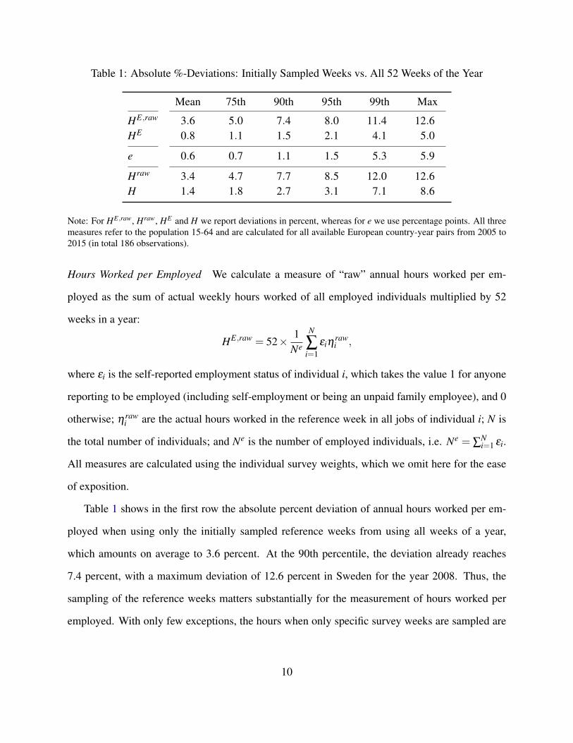
Table 1: Absolute %-Deviations: Initially Sampled Weeks vs. All 52 Weeks of the Year
Mean 75th 90th 95th 99th Max
HE,raw 3.6 5.0 7.4 8.0 11.4 12.6HE 0.8 1.1 1.5 2.1 4.1 5.0
e 0.6 0.7 1.1 1.5 5.3 5.9
Hraw 3.4 4.7 7.7 8.5 12.0 12.6H 1.4 1.8 2.7 3.1 7.1 8.6
Note: For HE,raw, Hraw, HE and H we report deviations in percent, whereas for e we use percentage points. All threemeasures refer to the population 15-64 and are calculated for all available European country-year pairs from 2005 to2015 (in total 186 observations).
Hours Worked per Employed We calculate a measure of “raw” annual hours worked per em-
ployed as the sum of actual weekly hours worked of all employed individuals multiplied by 52
weeks in a year:
HE,raw = 52× 1Ne
N
∑i=1
εiηrawi ,
where εi is the self-reported employment status of individual i, which takes the value 1 for anyone
reporting to be employed (including self-employment or being an unpaid family employee), and 0
otherwise; ηrawi are the actual hours worked in the reference week in all jobs of individual i; N is
the total number of individuals; and Ne is the number of employed individuals, i.e. Ne = ∑Ni=1 εi.
All measures are calculated using the individual survey weights, which we omit here for the ease
of exposition.
Table 1 shows in the first row the absolute percent deviation of annual hours worked per em-
ployed when using only the initially sampled reference weeks from using all weeks of a year,
which amounts on average to 3.6 percent. At the 90th percentile, the deviation already reaches
7.4 percent, with a maximum deviation of 12.6 percent in Sweden for the year 2008. Thus, the
sampling of the reference weeks matters substantially for the measurement of hours worked per
employed. With only few exceptions, the hours when only specific survey weeks are sampled are
10
larger than when all weeks of the year are sampled.6
Employment Rate The employment rate (e) is simply given by the number of employed individ-
uals divided by all individuals in the sample
e =Ne
N. (1)
Equation (1) is the employment to population ratio for the population 15-64, but we henceforth
refer to it as the employment rate.7 The third row of Table 1 shows that the employment rate
exhibits significantly less seasonality than the raw hours worked per employed measure. The
average absolute percentage point deviation between constructing the employment rate only based
on specific survey weeks relative to the entire year amounts to only 0.6 percentage points. At
the 90th percentiles, the difference is still relatively small with 1.1 percentage points. Moreover,
employment rates are not systematically higher (or lower) if only specific weeks are sampled than
if the entire year is sampled. There are only two country-year pairs for which the deviations are
larger than 5 percentage points, namely from Germany and Belgium. Both countries used only one
specific week as reference week (Germany until 2004, Belgium until 1998), suggesting that the
corresponding time-series of the employment rates have to be used with some caution.
Hours Worked per Person The fourth row of Table 1 finally shows the seasonality of hours
worked per person (Hraw), which is the product of hours worked per employed and the employ-
6This is the case for all countries in all but at most two years. The only exception are the Netherlands, where hoursare lower in the initially sampled weeks in seven out of eleven years.
7Online Appendix Section A.1.3 reports two alternative measures of the employment rate. The first alternativemeasure relies on defining employment based on usually working positive hours. This leaves the employment ratevirtually unchanged (see Table A.6). The second alternative measure involves a different definition of employmentfor women on maternity leave. This has only a modest impact on female employment rates, and is far too small todrive international differences in female employment rates (see Table A.7). Note that by construction, hours workedper person remain always the same no matter what definition is used for the employment rate, because an increase(decrease) in the alternative employment rate relative to our baseline definition is always offset by a decrease (increase)in the corresponding measure of hours worked per employed.
11
ment rate. The mean absolute deviation in hours worked per person between the initially sampled
weeks and all weeks of the year amounts to 3.4 percent, and at the 90th percentile it already reaches
8.5 percent.8 Thus, the strong seasonality of hours worked per employed is fully reflected in hours
worked per person.
Challenge 2: Underreporting of Vacation Weeks
For most European countries all weeks of the year are sampled from 2005 onwards. If each week
would be sampled with equal probability and cover a representative sample of the population week
by week (rather than only over the entire year), then average vacation weeks should be captured ac-
curately in the labor force surveys, and one could compute average annual hours worked simply by
summing up average weekly hours worked in each week over all 52 weeks of the year. Calculating
the average number of vacation weeks from the micro data yields an average of 3.4 “self-reported”
vacation weeks in Europe, defining vacation as the sum of public holidays and annual leave.9
Given that public holidays alone in all countries sum up to 1.5 to 2.5 weeks, these self-reported
weeks of annual leave and public holidays seem implausibly low. In fact, based on external data
sources (national statistical offices, unions, employer organizations, the European Industrial Rela-
tions Observatory, and the International Labor Organization), the average weeks of vacation over
the same time period for our sample of European countries amount to 6.8 weeks per year.10 Put
differently, even exploiting continuous year surveys and computing average actual hours over all
52 weeks of the year without any further adjustment (HE,raw) leads to a significant overestimate of
annual hours worked. Moreover, the size of the bias exhibits a substantial cross-country variation.
8The correlation between HE,raw and e is slightly negative (-0.045), which leads to slightly smaller absolute percentdeviations for Hraw than for HE,raw, except at the extremes.
9Table A.1.1 in Online Appendix A.2.2 reports the results for each country as well as the description of how weconstruct the self-reported vacation weeks.
10Online Appendix A.2.1 lists the exact external data sources and explains further assumptions in the constructionof the number of vacation weeks. It also shows that the time series variation in vacation weeks within each countryis small, with the notable exception of Denmark. For the US, the discrepancy between self-reported and externalvacation weeks is somewhat smaller but still substantial, with 1.3 vs. 3.7 weeks. We expect a discrepancy for the US,since weeks with major public holidays are not sampled.
12
To get a better understanding of the sources of this discrepancy, we investigate in more detail
the case of Germany, which features the largest difference among all countries, amounting to 5.1
weeks. While we provide all details in Online Appendix Section A.2.2, our results of this analysis
can be summarized as follows. First, using the German Socio-Economic Panel, Schnitzlein (2011)
reports that on average 3 of the average 31 entitled days of annual leave per year go unused. Thus,
the underusage of entitled leave can explain only a very small portion of the discrepancy of 5.1
weeks between self-reports and official vacation days. Second, not all weeks are sampled with the
same probability in the EU LFS, see Figure A.1 in Online Appendix Section A.2.2. For exam-
ple, the reference week which contains Christmas day is on average sampled with a probability of
0.7%, significantly below the 1.9% that would be implied by equal sampling. Third, the German
Statistical Office also has some evidence that respondents might dislike using a vacation week as
a reference week, either because they are too busy the first week after a vacation to fill out the
questionnaire, or because they perceive it as “inappropriate” to use a vacation week as reference
week. Summarizing, at least for Germany there exists evidence of underreporting of days of an-
nual leave and public holidays in the EU LFS even after the introduction of continuous sampling
over the entire year. It seems at least not implausible that these factors can explain the discrep-
ancies between the self-reported and external vacation weeks for the remaining countries as well.
Therefore, it is important to adjust hours worked per employed for vacation using external data
even when analyzing the recent cross-section from 2005 onwards, when all weeks of a year are
sampled.
Measurement of Hours Worked per Employed
As documented so far, the raw measure of hours worked per employed suffers from two weak-
nesses: first, seasonality in hours worked per employed impedes the comparability of hours worked
across countries and within European countries over time because of differences in the sampled
reference weeks; second, vacation weeks are underreported in the labor force surveys even if all
13

weeks of a year are sampled. We therefore apply the following adjustment to construct a measure
of hours worked per employed that overcomes both weaknesses: we first obtain individual hours
worked in a non-vacation week, i.e. a typical work week without a reduction in work time be-
cause of a public holiday or annual leave, and then require consistency of annual leave and public
holidays in the micro data with the country-wide average. This closely follows Pilat (2003).
To calculate hours worked in a non-vacation week ηi for each employed individual, we use as a
baseline actual hours worked in all jobs in the reference week. However, if a respondent indicates
that he/she worked less hours than usual in the main job in the reference week, and states as the
main reason for doing so public holidays or annual leave, we replace weekly hours by usual hours
in the main job plus actual hours worked in all additional jobs.11 Thus,
ηi =
usual hours in main job if actual hours in main job<usual hours in main job
+ actual hours in all additional jobs because of annual leave or public holiday
actual hours in all jobs ηrawi otherwise.
We refer to these hours ηi as “hours worked in a non-vacation week”. Averaging over our popula-
tion of interest yields mean weekly hours worked in a non-vacation week h, i.e.
h =1
Ne
N
∑i=1
εiηi. (2)
If people work less hours than usual for other reasons than vacations, e.g. because of sickness,
or more hours than usual because of overtime, this is captured by this measure. Figure 2 shows
11Note that respondents can only indicate one reason for working different hours than usual, and for additional jobswe do not have information on usual hours. One might be worried that individuals with multiple jobs might takevacation from their main job to work more hours in their additional job. However, in the US only about 6% of theemployed population hold multiple jobs, and about 3% on average in the European countries in our sample. Hence,any potential effects on our measure of aggregate hours worked should be negligible. In Online Appendix A.1.4 wediscuss some differences between the CPS and EU LFS questionnaire regarding the construction of our hours measure,which however have virtually no impact on the statistics presented in the paper.
14
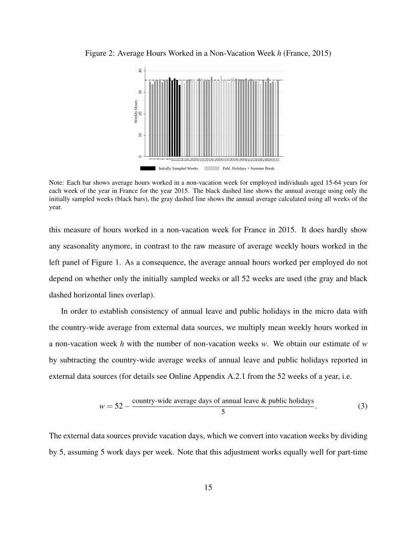
Figure 2: Average Hours Worked in a Non-Vacation Week h (France, 2015)
010
2030
40W
eekl
y H
ours
1 2 3 4 5 6 7 8 9 10 11 12 13 14 15 16 17 18 19 20 21 22 23 24 25 26 27 28 29 30 31 32 33 34 35 36 37 38 39 40 41 42 43 44 45 46 47 48 49 50 51 52 53
Initially Sampled Weeks Publ. Holidays + Summer Break
Note: Each bar shows average hours worked in a non-vacation week for employed individuals aged 15-64 years foreach week of the year in France for the year 2015. The black dashed line shows the annual average using only theinitially sampled weeks (black bars), the gray dashed line shows the annual average calculated using all weeks of theyear.
this measure of hours worked in a non-vacation week for France in 2015. It does hardly show
any seasonality anymore, in contrast to the raw measure of average weekly hours worked in the
left panel of Figure 1. As a consequence, the average annual hours worked per employed do not
depend on whether only the initially sampled weeks or all 52 weeks are used (the gray and black
dashed horizontal lines overlap).
In order to establish consistency of annual leave and public holidays in the micro data with
the country-wide average from external data sources, we multiply mean weekly hours worked in
a non-vacation week h with the number of non-vacation weeks w. We obtain our estimate of w
by subtracting the country-wide average weeks of annual leave and public holidays reported in
external data sources (for details see Online Appendix A.2.1 from the 52 weeks of a year, i.e.
w = 52− country-wide average days of annual leave & public holidays5
. (3)
The external data sources provide vacation days, which we convert into vacation weeks by dividing
by 5, assuming 5 work days per week. Note that this adjustment works equally well for part-time
15
and full-time workers. Part-time workers get the same number of vacation weeks as full-time
workers; the number of vacation hours are adjusted according to their part-time schedule. The
disadvantage of this procedure is that we rule out any heterogeneity in the number of days of
annual leave and public holidays. One implication of this is that individuals who work while being
on vacation, and thus only use a fraction of their vacation time, are assumed to take the full vacation
time as given by the country-wide average. Since we only observe each individual for one week of
the year, we cannot verify whether this assumption holds. To be precise, for individuals reporting
positive hours worked but less than usual hours because of vacation, we cannot distinguish whether
they took some days off in the reference week and only worked on the remaining days, or whether
they took the full week off but worked some hours while on vacation. To the extent that the latter
is the case, we are underestimating hours worked per person. In Online Appendix Section A.2.3,
we conduct a robustness check which allows for heterogeneous number of vacation weeks by
demographic subgroups. Specifically, we assume that the heterogeneity in self-reported vacation
weeks reflects the true degree of heterogeneity, but we still impose that the average number of
vacation weeks corresponds to the one from external sources. Allowing heterogeneity in vacation
weeks has only a negligible effect on our results.
The second row of Table 1 shows the deviation of the annual hours worked per employed
measure (HE = h×w) if only the initially sampled survey weeks are used as reference weeks,
compared to all weeks of the year. While for the “raw” measure of hours worked per employed in
the first row the mean absolute percent deviation amounts to 3.6 percent, the mean absolute percent
deviation of our measure of hours worked per employed is with 0.8 percent substantially smaller.
Thus, externally adjusting for vacation is successful in insuring comparability of the data over
time. This becomes apparent for the example of France in the year 2015 by comparing Figures 1a
and 2. Only at the top end of the distribution, we still see a non-negligible effect of the sampling
of the reference weeks. The three countries with deviations in the top five percent are Belgium,
Norway, and Poland. As the last row of Table 1 shows, the deviations in hours worked per person
16

between the initially sampled weeks and all weeks of the year is also significantly reduced by
our adjustment procedure. The mean absolute deviation amounts to 1.4 percent, compared to 3.4
percent for the “raw” measure of hours worked per person. At the 95th percentile, the absolute
deviation is 3.1 percent, compared to 8.5 percent without the adjustment.12
Finally, while we document the need to adjust for hours lost due to public holidays and annual
leave, the same could in principle apply to working less hours than usual because of sick leave or
other reasons, and also to working more hours than usual (overtime and additional jobs). There
are two dimensions to this issue. First, in how far do such differences between usual and actual
hours vary with the set of reference weeks available? In Online Appendix Section A.3, we provide
evidence that none of the other reasons for working more or less time than usual vary with the
set of reference weeks. Put differently, with regard to these categories the initially sampled weeks
seem to be representative for the average over all weeks. Second, is there systematic under- or
overreporting of these categories? Unfortunately, sick days from external data sources are only
available for a subset of countries and years. For those country-year pairs, we find that the self-
reported number of sick days in our data are smaller than sick days from external data sources.
This is similar to our finding for vacation days. However, the discrepancy is on average smaller
than for vacation days and public holidays, with on average 1.1 weeks in Europe and 0.3 weeks in
the US, see Online Appendix Section A.3.
Comparison with NIPA Hours
As is common practice when working with micro data sets, see e.g. the 2010 Review of Economic
Dynamics special issue on “Cross Sectional Facts for Macroeconomists” (Krueger et al., 2010),
we compare our aggregate statistics on hours worked per person based on the labor force surveys
(LFS) with those from the National Income and Product Accounts (NIPA) as provided by the
12The correlation between HE and e is positive (0.095), which leads to larger absolute percent deviations for H thanfor HE .
17

Figure 3: Percent Deviations of Hours Worked and Employment in NIPA from LFS
(a) Hours Worked per Person−
10−
50
510
1520
25%
Dev
iatio
n of
NIP
A fr
om L
FS
Hou
rs p
er P
erso
n
US AT BE CH CZ DE DK ES FR GR HU IE IT NL NO PL PT SE UK
Hours per Person
(b) Empl. Rate and Hours Worked per Employed
−10
−5
05
1015
2025
% D
evia
tion
of N
IPA
from
LF
S
US AT BE CH CZ DE DK ES FR GR HU IE IT NL NO PL PT SE UK
Employment Rate Hours per Employed
Note: NIPA hours worked per person are calculated by dividing NIPA total hours from the OECD National Accountsby the population aged 15 to 64 from the OECD ALFS database. For the LFS data, total LFS hours (everyone agedolder than 15) are divided by the LFS popluation aged 15 to 64. The NIPA employment rate is calculated as totalemployment from the OECD National Accounts (domestic concept) divided by the population aged 15 to 64, whilethe LFS employment rate is total number of employed (older than 15) divided by the LFS population 15 to 64. Allnumbers are for the year 2012.
OECD’s “National Accounts Database”.13 Specifically, we calculate a NIPA measure of hours
worked per person by dividing NIPA total hours by the population aged 15 to 64 obtained from
the OECD’s “Annual Labour Force Statistics”. For the LFS data, we divide total LFS hours (rather
than only those by the population aged 15 to 64 as in the previous subsections) by the population
aged 15 to 64 directly taken from the LFS.
Figure 3a shows the average country-specific percent deviation of NIPA estimates for hours
worked per person from LFS estimates for 2012, the last year in which all data are available for
all countries. On average across all countries, hours worked per person are 43 hours (4.4 percent)
higher in the NIPA data than in the LFS data. In 6 out of 19 countries, the NIPA estimates are
below the LFS estimates (on average by -3.3 percent).14 Figure 3b shows that these differences
13An alternative data source for aggregate hours worked is the Conference Board’s “Total Economy Database”(TED). For the majority of countries and years in our sample the data from the OECD and the TED are exactly thesame, see Online Appendix C.2.
14To put these deviations between the NIPA hours and the LFS hours measures into perspective, the implied Europe-US hours worked per person difference (a key statistic our subsequent empirical analysis focuses on) for the year 2012amounts to -4.5% in NIPA data and -15.9% in LFS data. Hence, our data predict a much larger gap in absolute value
18
stem from disagreement between the two data sources for both the employment rate and hours
worked per employed. In contrast to the cross-section, we show in Online Appendix C.2 that the
time trends are generally much more similar between the two different data sources.
What can explain these cross-sectional differences between NIPA and LFS estimates? LFS
and NIPA data differ conceptually along two dimensions. First, LFS data cover only civilian, non-
institutionalized residents aged 15 and older, while NIPA data do not impose these restrictions to
ensure that the labor inputs are consistent with the measurement of gross domestic output (GDP).
Second, the NIPA estimates are usually constructed in country-specific ways from multiple data
sources (administrative data, social security data, employer surveys, labor force surveys, census
data, etc.). Online Appendix A.4 provides more details on both of these conceptual differences and
documents that the employment rate differences in Figure 3b cannot be reconciled with differences
in the covered population. For hours worked per employed, we cannot conduct such a comparison.
For the US, Abraham et al. (2013) document which features of the underlying data sources drive
the differences between NIPA and LFS employment rate estimates, and Eldridge et al. (2004) and
Frazis and Stewart (2010) do the same for hours works per employed. While the details are specific
to the US, these papers highlight that the NIPA estimates are not necessarily superior to the LFS
estimates, see Online Appendix A.4 for details. E.g., Ramey (2012) suggests that the LFS hours
yield a more accurate picture of the true work hours of individuals.
The combination of multiple data sources might deliver more accurate estimates of employment
and hours worked for a given country. The downside is that the cross-country comparability suffers,
despite the efforts to harmonize measurement through the Systems of National Accounts, see Fleck
(2009). In fact, the OECD remarks on its website that “The [hours worked] data are intended
for comparisons of trends over time; they are unsuitable for comparisons of the level of average
than the NIPA data. Most of the macro literature on hours worked cited in the introduction base their analysis on NIPAdata (or some variant of it). Comparing the facts reported in these papers among each other and to the facts reportedhere is however difficult, since the NIPA hours underwent massive revisions over time. In a companion paper, Bicket al. (2017), we document these revisions and show that they affect the measured Europe-US hours gap tremendously.
19

annual hours of work for a given year, because of differences in their sources,” and recommends
using employment rates based on labor force surveys for cross-country comparisons: “National
Labor Force Surveys are the best way to capture unemployment and employment according to the
ILO guidelines that define the criteria for a person to be considered as unemployed or employed...
While data from LFS make international comparisons easier compared to a mixture of survey and
registration data, there are some differences across countries in coverage, survey timing, etc, that
may affect international comparisons of labour market outcomes”.15 Our approach deals with one
of the main differences in the cross-country comparability of the LFS, namely the survey timing.16
In any case, only the LFS give us the opportunity to investigate Europe-US hours differences in
detail, since they allow to construct average hours for demographic subgroups.
III. The Aggregate Europe-US Hours Difference
In this section, we start using our harmonized data to document some basic facts for aggregate
hours worked differences between Europe and the US for the most recently available years (2013-
2015). These facts are hardly influenced by any persistent effects of the global financial crisis and
the European debt crisis. Focusing on the pre-crisis years 2005-2007 yields very similar results.
We restrict our attention to the population aged 15 to 64. Subsequently, we document the cross-
country differences for the three components of labor supply, namely the employment rate, weeks
worked, and weekly hours worked.
20

Figure 4: Average Hours Worked per Person
025
050
075
01,
000
1,25
0
USScandinavia
Western EuropeEastern Europe
Southern Europe
US SE NO DK CH UK AT DE NL BE FR IE CZ PL HU PT ES GR IT
Note: Average hours worked per person are calculated for the population aged 15 to 64 over the years 2013 to 2015.
Hours Worked per Person
Figure 4 shows hours worked per person in the LFS data on the country level by geographic
region. Within each region, we order countries by average hours worked per person. Switzerland,
the US, and the Czech Republic stand out with the highest hours worked per person, exceeding
1250, while Italians work less than 900 hours per year. Overall, mean hours worked per person in
Southern Europe are the lowest (952 hours), while the mean hours worked per person across the
other European regions are quite similar, ranging from 1098 hours in Western Europe to 1169 hours
in Eastern Europe. The implied Europe-US hours per person gap is 180 hours, or 14 percent.17
15Both quotes we retrieved from the OECD’s website on August 9, 2017: http://
stats.oecd.org/Index.aspx?DataSetCode=ANHRS and http://www.oecd.org/els/emp/
basicstatisticalconceptsemploymentunemploymentandactivityinlabourforcesurveys.htm.16Other reasons impeding the comparability across time and countries of the LFS, which we cannot adjust for, are
the revision of population figures used for population adjustment on the basis of new population censuses, as well aschanges in the sampling design, and content or order of the questionnaire. For details, see http://ec.europa.eu/eurostat/statistics-explained/index.php/EU_labour_force_survey (retrieved on August 9, 2017).
17We always report simple cross-country averages. Including also adults older than 64 increases the Europe-UShours gap to 19 percent.
21

Figure 5: Hours Worked Components
(a) Weekly Hours & Empl. Rate
US
CZHUPL
DK
NO
SEAT
BE CH
DE
FRIE
NL
UK
ES
GR
IT
PT
3133
3537
3941
43 W
eekl
y H
ours
50 55 60 65 70 75 80 Employment Rate (in %)
(b) Weeks Worked & Empl. Rate
US
CZ
HUPL
DK
NOSEAT
BE
CH
DE
FR
IE
NL
UK
ESGR
IT
PT
4344
4546
4748
49 W
eeks
Wor
ked
50 55 60 65 70 75 80 Employment Rate (in %)
(c) Weeks Worked & Weekly Hrs.
US
CZ
HUPL
DK
NOSEAT
BE
CH
DE
FR
IE
NL
UK
ESGR
IT
PT
4344
4546
4748
49 W
eeks
Wor
ked
31 33 35 37 39 41 43 Weekly Hours
Note: The dotted vertical and horizontal lines indicating median values for each variable, and the solid line representsa fitted OLS regression line. All variables are averages over the years 2013 to 2015. Weekly hours worked and theemployment rate are calculated for the population aged 15 to 64.
The Three Components of Hours Worked per Person
Average hours worked per person are the product of the employment rate and hours worked per em-
ployed, with the latter being the product of weekly hours worked per employed in a non-vacation
week and the number of weeks worked per year, i.e. H = e×h×w. Figure 5 shows how these three
components relate to each other and reveals interesting patterns of heterogeneity across regions,
despite the similar average hours worked per person across European regions. The five regions are
marked by different markers and colors, namely the US by a black x, Eastern Europe by a gray
circle, Scandinavia by black squares, Western Europe by black diamonds, and Southern Europe by
gray triangles.
Figure 5a plots weekly hours worked per employed in a non-vacation week (h) against the
employment rate (e), with the dotted vertical and horizontal lines indicating median values, and
the solid line representing a fitted OLS regression line. While hours worked per person do not
differ much on average across the European regions, with the exception of Southern Europe as
shown in Figure 4, a region-specific pattern for the relationship between the employment rate and
weekly hours emerges. Eastern and Southern European countries all have above median weekly
22

hours with Italy being the median country, but below median employment rates, with the exception
of the Czech Republic. The Scandinavian countries in turn have below median weekly hours and
above median employment rates. Weekly hours worked per employed in Western Europe are below
the median (the exceptions are Belgium and Switzerland), while the employment rates range from
below the median in Belgium, Ireland and France to the highest in Switzerland. Taken together,
a strong negative cross-country correlation between weekly hours worked per employed and the
employment rate of -0.55 arises: countries with high employment rates tend to feature low weekly
hours worked per employed in a non-vacation week, and vice versa.
Figure 5b plots the weeks worked (w) in a given country against the employment rate (e).
Weeks worked range in Europe from below 44 in Germany to 46.5 in the Netherlands, with most
of the cross-country variation coming from annual leave rather than public holidays (see Online
Appendix A.2.1). The US clearly stand out with more than 48 weeks worked per year. Overall, the
correlation between weeks worked and the employment rate is weak, amounting to -0.10 for all
countries and -0.17 if the US is excluded. Figure 5c plots weeks worked (w) against weekly hours
worked in a non-vacation week (h). The correlation between both variables is 0.28 and drops
to 0.21 once the US is excluded, which is consistent with the evidence in Altonji and Oldham
(2003). The weak correlations between weeks worked and employment rates or hours worked
might suggest that more public holidays or annual leave, i.e. less weeks worked per year, neither
induce more people to work nor to work longer hours during a non-vacation week.18
IV. Decomposing the Europe-US Hours Difference
We now exploit the richness of our micro data and move beyond the aggregate hours worked dif-
ferences between Europe and the US and provide “new answers” regarding the origins of these
differences. Specifically, we are interested in how important differences in the demographic com-
18There exists a strong negative correlation of -0.83 between weekly hours and the part-time rate, defined as thefraction of employed working less than 30 usual weekly hours. Thus, low weekly hours are driven by a large fractionof part-time workers, and vice versa.
23

position are for the aggregate patterns, and which groups are the main drivers of the aggregate pat-
terns. We proceed in two steps. First, in Subsection IV.1 we conduct a decomposition that analyzes
the extent to which different demographic compositions and differences in the three components of
labor supply contribute to the aggregate Europe-US hours difference. Second, in Subsection IV.2
we analyze whether the stark differences across countries in employment rates and weekly hours
worked are driven only by the behavior of specific demographic subgroups, or are prevalent across
all groups.
Decomposition by Demographics and Components of Hours Worked
Countries in our sample differ not only in the three components of hours worked, but also in their
demographic structure, i.e. the composition of the population by demographic characteristics. We
take into account three demographic characteristics, namely gender, age, and education, as well as
the sectoral composition of employment in a country. Explicitly accounting for these groups, we
write aggregate hours worked per person in country c as
Hc = wc ×J
∑j
f cj ec
j ×K
∑k
hcj,ksc
j,k, (4)
where j represents a set of demographic characteristics and k the sector of employment. wc are the
weeks worked (non-vacation weeks), f cj is the fraction of individuals with a given set of character-
istics j (with ∑Jj=1 f c
j = 1), ecj is the employment rate of group j, hc
j,k are the weekly hours worked
per employed in a non-vacation week by group j in sector k, an scj,k is the share of employed
individuals of group j working in sector k (with ∑Kk=1 sc
j,k = 1). Each group j is defined by the
interaction of one of three age groups (15-24, 25-54, 55-64), three education groups (low, medium,
high), and gender.19 Only for the young age group, we allow a fourth educational category “still
19The different levels of education are defined according to the ISCED classifications, with “low” correspondingto lower secondary education, “medium” to upper secondary education, and “high” comprising any tertiary educationdegree. For example, for the US “low” corresponds to less than high school education, “medium” to completed highschool education, and “high” to having at least an associate’s degree.
24
enrolled in education”. Since only employed individuals can be allocated to a sector, the sectoral
composition only affects hours worked per employed, not the employment rate. We consider three
broad sectors: services, manufacturing, and agriculture.20 Last, remember that in the baseline
analysis we assume the same number of weeks worked for everyone. In Online Appendix Table
B.5 we show that relaxing this assumption has only a negligible effect on our results.
To quantify the contribution of the three components of labor supply, the demographic compo-
sition, and the sectoral composition to the difference of the country-specific hours relative to the
US, we calculate counterfactual hours by setting for every country one of these five features after
the other equal to the corresponding US value. We then measure the incremental fraction of the
aggregate hours worked per person difference relative to the US accounted for by this feature.21
The quantitative results depend on the order in which the features are set country specific. With
five features, there are 120 different possible orderings. Here, we report the mean results over all
120 different orderings, and in Online Appendix Table B.4 the minimum and maximum from all
120 different orderings. This decomposition is similar in spirit to the one done by Blundell et al.
(2011, 2013) for time-trends in hours in France, the UK, and the US. Note that this is a statistical
decomposition, not to be interpreted as a causal analysis, since the different components entering
the decomposition are clearly endogenous variables and determined jointly.
Figure 6 shows the results from our decomposition exercise. Specifically, we show how the
difference in hours worked per person to the US is divided into the fraction accounted for by
weeks worked w, the demographic composition f , employment rates e, weekly hours h, and the
sectoral composition s. A negative entry indicates that a factor does not positively contribute to the
overall difference, but implies higher hours in the European region than in the US. To facilitate the
20On average across countries and years 2013 to 2015 the educational status is missing for 0.5 percent of individ-uals and the sector of employment is missing for 0.7 percent of the employed. The corresponding maxima are 3.7percent for Denmark in 2013, and 7.3 percent for the Netherlands in 2013, respectively. For consistency our decompo-sition analysis thus features in fact a fifth educational category and fourth sectoral category representing the missingobservations.
21Online Appendix Section B.1 describes the procedure in detail focusing only on the three components of laborsupply analyzed in the previous subsection.
25
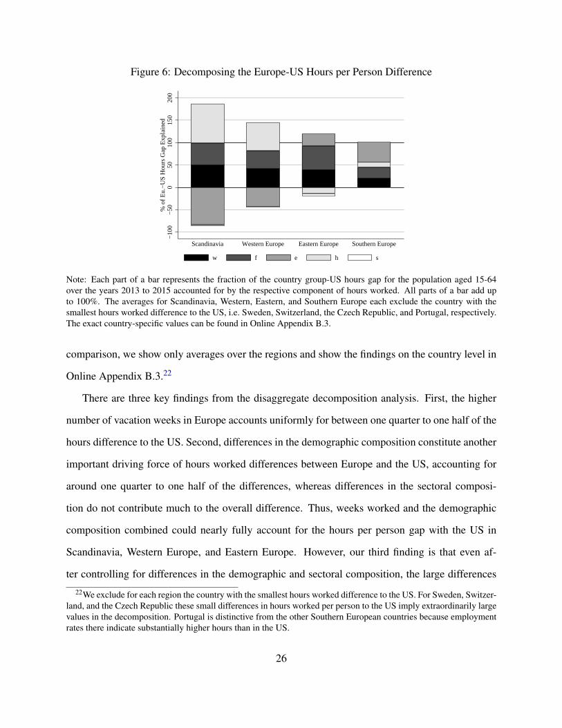
Figure 6: Decomposing the Europe-US Hours per Person Difference
−10
0−
500
5010
015
020
0%
of E
u.−
US
Hou
rs G
ap E
xpla
ined
Scandinavia Western Europe Eastern Europe Southern Europe
w f e h s
Note: Each part of a bar represents the fraction of the country group-US hours gap for the population aged 15-64over the years 2013 to 2015 accounted for by the respective component of hours worked. All parts of a bar add upto 100%. The averages for Scandinavia, Western, Eastern, and Southern Europe each exclude the country with thesmallest hours worked difference to the US, i.e. Sweden, Switzerland, the Czech Republic, and Portugal, respectively.The exact country-specific values can be found in Online Appendix B.3.
comparison, we show only averages over the regions and show the findings on the country level in
Online Appendix B.3.22
There are three key findings from the disaggregate decomposition analysis. First, the higher
number of vacation weeks in Europe accounts uniformly for between one quarter to one half of the
hours difference to the US. Second, differences in the demographic composition constitute another
important driving force of hours worked differences between Europe and the US, accounting for
around one quarter to one half of the differences, whereas differences in the sectoral composi-
tion do not contribute much to the overall difference. Thus, weeks worked and the demographic
composition combined could nearly fully account for the hours per person gap with the US in
Scandinavia, Western Europe, and Eastern Europe. However, our third finding is that even af-
ter controlling for differences in the demographic and sectoral composition, the large differences
22We exclude for each region the country with the smallest hours worked difference to the US. For Sweden, Switzer-land, and the Czech Republic these small differences in hours worked per person to the US imply extraordinarily largevalues in the decomposition. Portugal is distinctive from the other Southern European countries because employmentrates there indicate substantially higher hours than in the US.
26

across Europe in the relative contribution of employment rates and weekly hours in accounting for
the hours difference to the US persist. For Scandinavia and Western Europe, lower weekly hours
worked account for slightly less than 90 percent and slightly more than 60 percent, respectively, of
the lower hours per person than in the US. The employment rate differences in turn would predict
hours per person differences of a similar magnitude but with the opposite sign. The opposite is true
for Eastern Europe, with employment rate differences accounting for roughly one quarter of the
hours per person gap with the US, and weekly hours predicting higher hours than in the US. Only
in Southern Europe, employment rate (slightly less than 50 percent) and weekly hours (slightly
more than 10 percent) differences both contribute positively to the hours gap to the US.
Before investigating which demographic groups differ in their labor supply behavior and are
thus driving the remaining differences attributable to employment rates and weekly hours worked,
we show why the demographic composition is so important in accounting for the Europe-US hours
gap, and why the sectoral composition is not. From a conceptual perspective, the demographic and
sectoral compositions matter in the decomposition analysis only if two conditions are met: first,
the composition across countries needs to be different; second, the demographic groups need to
exhibit either different employment rates or different weekly hours worked within a country.
With regard to the composition, since in all sample countries and years women make up around
50 percent of the population aged 15 to 64, applying the gender composition of the US to a coun-
try will not affect the corresponding counterfactual estimate of aggregate hours worked per person.
The same holds true for the age composition, which is relatively similar across countries as well
(see Online Appendix Figure B.1). The educational and sectoral composition in turn vary signif-
icantly across countries. The left panel of Figure 7 shows that the US stands out with the lowest
share of low educated individuals with less than 10 percent, compared to nearly 40 percent in
Southern Europe. The reversed pattern prevails for high educated individuals, while the fraction of
young adults still enrolled in education is rather similar across regions.
The right panel of Figure 7 shows the sectoral composition across regions. The share of em-
27

Figure 7: Demographic Structure
(a) Educational Composition0
1020
3040
5060
7080
USScandinavia
Western EuropeEastern Europe
Southern Europe
Still Enrolled Low
Medium High
(b) Sectoral Composition
010
2030
4050
6070
80
USScandinavia
Western EuropeEastern Europe
Southern Europe
Agriculture Manufacturing
Services
Note: Each bar shows for the years 2013 to 2015 (a) the fraction (in %) of the 15 to 64 year old population in eacheducation category; (b) the fraction (in %) of the 15 to 64 year old employed population in each sectoral category.
ployed people working in services is highest in the US with about 80 percent and lowest in Eastern
Europe with around 60 percent. The low share in services in Eastern and Southern Europe is off-
set by both a higher share of individuals working in manufacturing, and a slightly higher share
working in agriculture, with the latter being quite low everywhere.
While the sectoral and the educational compositions thus differ significantly across countries,
this only has an effect in the disaggregate decomposition if different educational groups show
different labor market behavior within a country, and individuals in different sectors work different
hours. Panels (a) to (d) in Figure 8 demonstrate why the large differences in the educational
composition accounts for a large fraction of the Europe-US hours gap. The differences in weekly
hours worked (panels (c) and (d)) by low, medium, and high educated individuals within a country
are rather small, but the differences in employment rates are substantial. On average across all
countries, medium educated individuals have a 21 percentage points higher employment rate than
low educated individuals, but a 10 percentage points lower one than high educated individuals.
Thus, the large differences in educational shares between Europe and the US, and in employment
rates by education within countries account for around one third to one half of the Europe-US
hours gap.
28

Figure 8: Labor Supply Broken Down by Education or Sector
(a) Employment Rate:
Low & Medium Educated
US
CZHU
PL
DKNOSE
AT
BE
CH
DE
FR
IE
NLUK
ESGRIT
PT
3040
5060
7080
90L
ow E
duca
tion
30 40 50 60 70 80 90Medium Education
(b) Employment Rate:
High & Medium Educated
US
CZ
HU
PL DK
NOSE
ATBE
CHDE
FRIE
NLUK
ES
GR
IT
PT
3040
5060
7080
90H
igh
Edu
catio
n
30 40 50 60 70 80 90Medium Education
(c) Weekly Hours:
Low & Medium Educated
US
CZHU
PL
DK
NO
SE
ATBECH
DE
FR
IE
NL
UK
ES
GR
IT
PT
3035
4045
5055
Low
Edu
catio
n
30 35 40 45 50 55Medium Education
(d) Weekly Hours:
High & Medium Educated
US CZHU
PL
DK
NO
SE
ATBE
CH
DE FR
IENL
UK ES
GR
IT
PT
3035
4045
5055
Hig
h E
duca
tion
30 35 40 45 50 55Medium Education
(e) Weekly Hours:
Agriculture & Manufacturing
USCZ
HU
PLDK
NO
SE
AT
BE
CH
DEFR
IE
NL
UK
ESGRIT PT
3035
4045
5055
Agr
icul
ture
30 35 40 45 50 55Manufacturing
(f) Weekly Hours:
Services & Manufacturing
USCZHU
PL
DKNO
SEATBE
CH
DE
FR
IE
NL
UKES
GR
IT
PT
3035
4045
5055
Serv
ices
30 35 40 45 50 55Manufacturing
Panels (a) and (b) plot the country-specific employment rates for different levels of education against each other. Panels(c) and (d) do the same for weekly hours. Panels (e) and (f) compare average weekly hours for different sectors. Eachaverage is calculated for the population aged 15 to 64 for 2013 to 2015. The dash-dotted line is the 45 degree line.
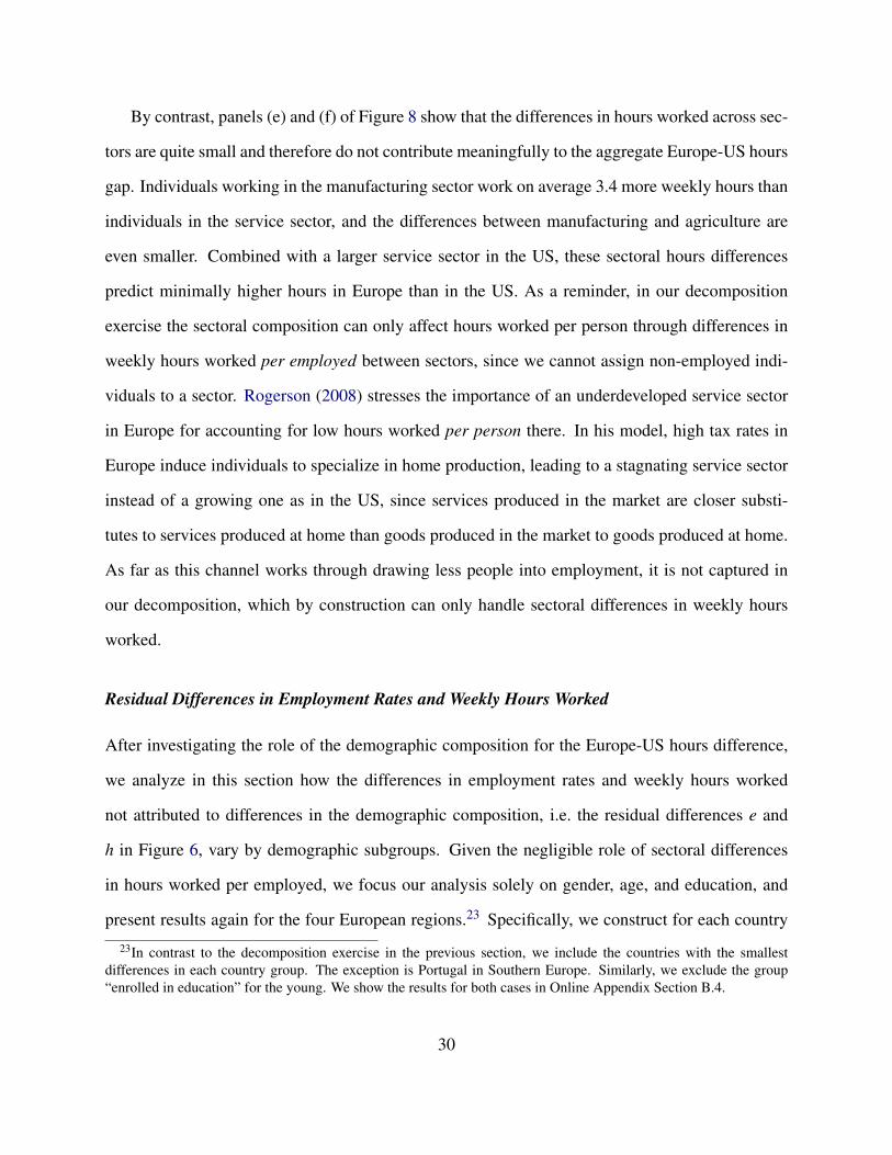
By contrast, panels (e) and (f) of Figure 8 show that the differences in hours worked across sec-
tors are quite small and therefore do not contribute meaningfully to the aggregate Europe-US hours
gap. Individuals working in the manufacturing sector work on average 3.4 more weekly hours than
individuals in the service sector, and the differences between manufacturing and agriculture are
even smaller. Combined with a larger service sector in the US, these sectoral hours differences
predict minimally higher hours in Europe than in the US. As a reminder, in our decomposition
exercise the sectoral composition can only affect hours worked per person through differences in
weekly hours worked per employed between sectors, since we cannot assign non-employed indi-
viduals to a sector. Rogerson (2008) stresses the importance of an underdeveloped service sector
in Europe for accounting for low hours worked per person there. In his model, high tax rates in
Europe induce individuals to specialize in home production, leading to a stagnating service sector
instead of a growing one as in the US, since services produced in the market are closer substi-
tutes to services produced at home than goods produced in the market to goods produced at home.
As far as this channel works through drawing less people into employment, it is not captured in
our decomposition, which by construction can only handle sectoral differences in weekly hours
worked.
Residual Differences in Employment Rates and Weekly Hours Worked
After investigating the role of the demographic composition for the Europe-US hours difference,
we analyze in this section how the differences in employment rates and weekly hours worked
not attributed to differences in the demographic composition, i.e. the residual differences e and
h in Figure 6, vary by demographic subgroups. Given the negligible role of sectoral differences
in hours worked per employed, we focus our analysis solely on gender, age, and education, and
present results again for the four European regions.23 Specifically, we construct for each country
23In contrast to the decomposition exercise in the previous section, we include the countries with the smallestdifferences in each country group. The exception is Portugal in Southern Europe. Similarly, we exclude the group“enrolled in education” for the young. We show the results for both cases in Online Appendix Section B.4.
30
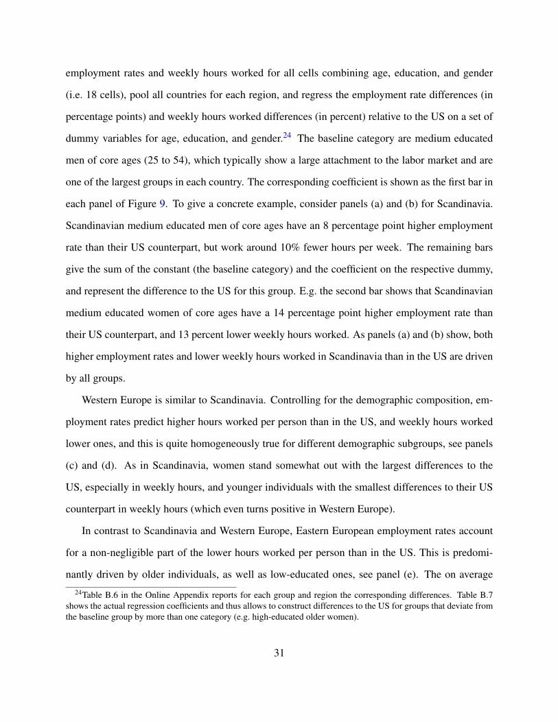
employment rates and weekly hours worked for all cells combining age, education, and gender
(i.e. 18 cells), pool all countries for each region, and regress the employment rate differences (in
percentage points) and weekly hours worked differences (in percent) relative to the US on a set of
dummy variables for age, education, and gender.24 The baseline category are medium educated
men of core ages (25 to 54), which typically show a large attachment to the labor market and are
one of the largest groups in each country. The corresponding coefficient is shown as the first bar in
each panel of Figure 9. To give a concrete example, consider panels (a) and (b) for Scandinavia.
Scandinavian medium educated men of core ages have an 8 percentage point higher employment
rate than their US counterpart, but work around 10% fewer hours per week. The remaining bars
give the sum of the constant (the baseline category) and the coefficient on the respective dummy,
and represent the difference to the US for this group. E.g. the second bar shows that Scandinavian
medium educated women of core ages have a 14 percentage point higher employment rate than
their US counterpart, and 13 percent lower weekly hours worked. As panels (a) and (b) show, both
higher employment rates and lower weekly hours worked in Scandinavia than in the US are driven
by all groups.
Western Europe is similar to Scandinavia. Controlling for the demographic composition, em-
ployment rates predict higher hours worked per person than in the US, and weekly hours worked
lower ones, and this is quite homogeneously true for different demographic subgroups, see panels
(c) and (d). As in Scandinavia, women stand somewhat out with the largest differences to the
US, especially in weekly hours, and younger individuals with the smallest differences to their US
counterpart in weekly hours (which even turns positive in Western Europe).
In contrast to Scandinavia and Western Europe, Eastern European employment rates account
for a non-negligible part of the lower hours worked per person than in the US. This is predomi-
nantly driven by older individuals, as well as low-educated ones, see panel (e). The on average
24Table B.6 in the Online Appendix reports for each group and region the corresponding differences. Table B.7shows the actual regression coefficients and thus allows to construct differences to the US for groups that deviate fromthe baseline group by more than one category (e.g. high-educated older women).
31

Figure 9: Differences between Europe and the US by Demographic Group
(a) Scandinavia: Empl. Rates
−25
−20
−15
−10
−5
05
1015
Baseline Female Young Old Low High
(b) Scandinavia: Weekly Hours
−25
−20
−15
−10
−5
05
1015
Baseline Female Young Old Low High
(c) Western Europe: Empl. Rates
−25
−20
−15
−10
−5
05
1015
Baseline Female Young Old Low High
(d) Western Europe: Weekly Hours
−25
−20
−15
−10
−5
05
1015
Baseline Female Young Old Low High
(e) Eastern Europe: Empl. Rates
−25
−20
−15
−10
−5
05
1015
Baseline Female Young Old Low High
(f) Eastern Europe: Weekly Hours
−25
−20
−15
−10
−5
05
1015
Baseline Female Young Old Low High
(g) Southern Europe: Empl. Rates
−25
−20
−15
−10
−5
05
1015
Baseline Female Young Old Low High
(h) Southern Europe: Weekly Hours
−25
−20
−15
−10
−5
05
1015
Baseline Female Young Old Low High
Note: The graphs show results from a regression of employment rate differences (in percentage points, left panels)and weekly hours worked differences (in percent, right panels) between different European regions and the US, brokendown by gender, age, and education, on a female dummy, dummies for young (15-24 years) and old (55-64 years), anddummies for low and high education. The regressions are run separately by region, and Portugal and the educationalcategory “still enrolled” are excluded. The white bars and gray dashed lines show the estimated constant, representingthe average difference for men aged 25-54 with medium education. The other graphs reflect the sum of the constantand the coefficients for the different dummies. The exact regression results can be found in Table B.7. All results arefor the years 2013 to 2015.
higher weekly hours worked in Eastern Europe compared to the US originate mostly from women,
the young, and the low educated. Among all country groups, the residual differences in Eastern
Europe are the most heterogeneous across different demographic groups.
Southern Europe (excluding Portugal) is the only region in which both employment rates and
weekly hours contribute positively to the lower hours worked per person than in the US. As panels
(g) and (h) show, this is again quite homogeneously true for all groups, except for the low educated.
Low educated core aged men exhibit higher employment rates and higher weekly hours than their
US counterparts. However, remember that the share of low educated individuals is exceptionally
high in Southern Europe. Thus, there is likely a more positive selection into this group than in the
US. At the same time, the young stand out with exceptionally low employment rates compared to
the US, a result of the high youth unemployment rates in Southern European countries.
Summing up the patterns across groups and regions, we find that for Scandinavia, Western
Europe, and Southern Europe the basic patterns are quite homogeneous across groups: in Scandi-
navia and Western Europe, all groups tend to exhibit higher employment rates and lower weekly
hours than their US counterparts. However, being female increases the differences to the US in
both margins. In Southern Europe, all demographic groups tend to exhibit both lower employment
rates and lower weekly hours than their US counterparts, with the exception of the low educated.
Eastern Europe features more heterogeneities across the groups than the other regions. This might
partly be due to a transition effect after the abolishment of socialism. E.g. older individuals stand
out with low employment rates and low hours, which could be due to a skill mismatch after the
transition.
V. Conclusion
This paper constructs “new data” on hours worked per person for the US and 18 European countries
from national labor force surveys for the years 1983 through 2015. While using labor force survey
data for cross-country studies of employment and hours worked is not “new”, our contribution
33

is to apply the harmonization procedure suggested by Pilat (2003), and to systematically analyze
its importance. This harmonization procedure addresses the two main challenges for measuring
hours worked consistently across countries and over time from labor force surveys: the different
sampling of reference weeks over the year, and the underreporting of vacation weeks. We show
that we overcome both problems by obtaining hours worked in a non-vacation week, i.e. a work
week without a reduction in work time because of a public holiday or annual leave, and requiring
consistency of annual leave and public holidays in the micro data with the country-wide average.
The richness of our micro data allows us to move beyond the aggregate hours worked differ-
ences between Europe and the US and to provide “new answers” regarding the origins of these
differences. We provide a decomposition of the Europe-US hours gap into the roles played by
weeks worked, employment rates, weekly hours worked per employed in a non-vacation week,
and the demographic and sectoral compositions. Weeks worked and the demographic composi-
tion, driven by the educational composition, both account for between one quarter and one half
of the lower hours per person in Europe than in the US. In addition, lower weekly hours worked
are important drivers of the lower hours in Scandinavia and Western Europe, where employment
rates alone would imply higher hours per person than in the US. These differences are present for
all demographic groups considered in our analysis, with women showing the largest differences.
For Eastern Europe, employment rate differences account for roughly one quarter of the hours
per person gap with the US, while weekly hours predict higher hours than in the US. Only in
Southern Europe (excluding Portugal), employment rate and weekly hours differences both con-
tribute positively to the hours gap to the US, with employment rates being much more important.
All demographic groups tend to exhibit both lower employment rates and lower weekly hours in
Southern Europe than their US counterparts, with the exception of the low educated.
Our results indicate new avenues for the research agenda of the study of hours worked dif-
ferences across Europe and the US. First, they show that the higher number of vacation weeks in
Europe is a significant driver of lower hours, and that longer vacation weeks are hardly associated
34

with either higher employment rates or longer weekly hours worked. This might indicate that the
number of work weeks is determined by other driving factors than those determining employment
rates and weekly hours worked, and raises the question whether they should be modeled as a choice
variable for the individual. One could instead follow e.g. a specification as in Kaplan (2012), which
takes the number of work weeks as exogenously given. Second, the educational composition mat-
ters significantly in accounting for cross-country differences in hours worked through its effect
on employment rates. Understanding why different education groups exhibit markedly different
employment rates but similar weekly hours worked, and why different countries feature very dif-
ferent educational compositions, will thus be a helpful step in understanding the origins of hours
worked differences across countries. For example, Restuccia and Vandenbroucke (2014) analyze
the role of longevity and economic growth for educational attainment and hours worked. Guvenen
et al. (2014) show that progressive taxation distorts the incentives to invest in human capital, and
differences in progressivity across countries can explain a sizable part of the differences in the
Europe-US hours per person gap for men. However, since these papers do not distinguish between
both margins, their theories remain silent about the very different education gradients between em-
ployment and hours worked per employed. Other candidate explanations affecting the incentives
to work differentially by education are welfare systems, or different degrees of regulations in the
labor markets for low and high educated, e.g. due to a minimum wage being binding for the poor.
Yet, one would have to investigate whether these factors influence the extensive margin more than
the intensive one.
References
Abraham, K. G., J. Haltiwanger, K. Sandusky, and J. R. Spletzer (2013). Exploring Differences inEmployment between Household and Establishment Data. Journal of Labor Economics 31(2),S129–S172.
Alesina, A., E. Glaeser, and B. Sacerdote (2005). Work and Leisure in the United States andEurope: Why So Different? NBER Macroeconomics Annual 20, 1–64.
35

Alonso-Ortiz, J. (2014). Social Security and Retirement Across the OECD. Journal of EconomicDynamics & Control 47, 300–316.
Altonji, J. G. and J. Oldham (2003). Vacation laws and annual work hours. Economic Perspec-tives Federal Reserve Bank of Chicago, Fall, 19–29.
Bick, A., B. Bruggemann, and N. Fuchs-Schundeln (2017). A Note on Data Revisions of Aggre-gate Hours Worked Series: Implications for the Europe-US Hours Gap. Working Paper.
Bick, A. and N. Fuchs-Schundeln (2017). Taxation and Labor Supply of Married Couples AcrossCountries: A Macroeconomic Analysis. Review of Economic Studies forthcoming.
Bick, A., N. Fuchs-Schundeln, and D. Lagakos (2018). How Do Hours Worked Vary with Income?Cross-Country Evidence and Implications. American Economic Review 108(1), 170–199.
Blundell, R., A. Bozio, and G. Laroque (2011). Labour supply and the extensive margin. AmericanEconomic Review: Papers & Proceedings.
Blundell, R., A. Bozio, and G. Laroque (2013). Extensive and Intensive Margins of Labour Supply:Work and Working Hours in the US, the UK and France. Fiscal Studies 34, 1–29.
Bridgman, B., G. Duernecker, and B. Herrendorf (2017). Structural Transformation, Marketiza-tion, and Household Production Around the World. Working Paper.
Burda, M., D. Hammermesh, and P. Weil (2008). Working Hours and Job Sharing in the EU andUSA, Chapter The Distribution of Total Work in the EU and the US.
Burda, M., D. Hammermesh, and P. Weil (2013). Total Work and Gender: Facts and PossibleExplanations. Journal of Population Economics 26(1), 239–161.
Eldridge, L. P., M. E. Manser, and P. F. Otto (2004). Alternative measures of supervisory employeehours and productivity growth. Monthly Labor Review April, 9–28.
Erosa, A., L. Fuster, and G. Kambourov (2012). Labor Supply and Government Programs: ACross-Country Analysis. Journal of Monetary Economics 59, 84–107.
Faggio, G. and S. Nickell (2007). Patterns of Work Across the OECD. Economic Journal 117,F416–F440.
Fang, L. and C. McDaniel (2017). Home Hours in the United States and Europe. B.E. Journal ofMacroeconomics: Advances 17(1), 1–27.
Fleck, S. E. (2009, May). International Comparisons of Hours Worked: An Assessment of Statis-tics. Monthly Labor Review 132(5), 3–31.
Frazis, H. and J. Stewart (2010). Why Do BLS Hours Series Tell Different Stories About Trendsin Hours Worked? BLS Working Paper 433.
36
Guvenen, F., B. Kuruscu, and S. Ozkan (2014). Taxation of Human Capital and Wage Inequality:A Cross-Country Analysis. Review of Economic Studies 81, 818–850.
Kaplan, G. (2012). Inequality and the Life Cycle. Quantitative Economics 3, 471–525.
Krueger, D., F. Perri, L. Pistaferri, and G. L. Violante (2010). Cross-Sectional Facts for Macroe-conomists. Review of Economic Dynamics 13(1), 1–14.
McDaniel, C. (2011). Forces Shaping Hours Worked in the OECD, 1960-2004. American Eco-nomic Journal: Macroeconomics 3, 27–52.
Ohanian, L. and A. Raffo (2012). Aggregate Hours Worked in OECD Countries: New Measure-ment And Implications for Business Cycles. Journal of Monetary Economics 59(1), 40–56.
Olovsson, C. (2009). Why Do Europeans Work So Little? International Economic Review 50(1),39–61.
Pilat, D. (2003). Measuring Hours Worked in OECD Countries. DSTI/EAS/IND/SWP(2003)10,OECD.
Prescott, E. C. (2004). Why Do Americans Work So Much More Than Europeans? FederalReserve Bank of Minneapolis Quarterly Review 28, 2–13.
Ramey, V. A. (2012). The Impact of Hours Measures on the Trend and Cyclical Behavior of U.S.Labor Productivity. Working paper, University of California San Diego.
Restuccia, D. and G. Vandenbroucke (2014). Explaining Educational Attainment across Countriesand over Time. Review of Economic Dynamics 17(4), 824–841.
Rogerson, R. (2006). Understanding Differences in Hours Worked. Review of Economic Dynam-ics 9, 365–409.
Rogerson, R. (2008). Structural Transformation and the Deterioration of European Labor MarketOutcomes. Journal of Political Economy 116, 235–259.
Schnitzlein, D. D. (2011). Umfang und Folgen der Nichtinanspruchnahme von Urlaub in Deutsch-land. DIW Wochenbericht 51+52, 14–20.
Wallenius, J. (2013). Social Security and Cross-Country Differences in Hours: A General Equi-librium Analysis. Journal of Economic Dynamics and Control 37, 2466–2482.
37