House Price Beliefs And Mortgage Leverage Choice∗

Michael Bailey† Eduardo Dávila‡ Theresa Kuchler§ Johannes Stroebel¶

Abstract

We study the relationship between homebuyers’ beliefs about future house price changes and theirmortgage leverage choices. Whether more pessimistic homebuyers choose more or less leverage dependson their willingness to reduce the size of their housing investments. When households primarilymaximize the levered return of their property investments, more pessimistic homebuyers reduce theirleverage to purchase smaller houses. On the other hand, when considerations such as family size pindown the desired property size, pessimistic homebuyers reduce their financial exposure to the housingmarket by making smaller downpayments to buy similarly-sized homes. To determine which scenariobetter describes the data, we investigate the cross-sectional relationship between house price beliefsand mortgage leverage choices in the U.S. housing market. We exploit plausibly exogenous variationin house price beliefs to show that more pessimistic homebuyers make smaller downpayments andchoose higher leverage, in particular in states where default costs are relatively low, as well as duringperiods when house prices are expected to fall on average. Our results highlight the important role ofheterogeneous beliefs in explaining households’ financial decisions.

JEL Codes: E44, G12, D12, D84, R21Keywords: Leverage, Mortgage Choice, Disagreement, Heterogeneous Beliefs, Collateralized Credit

∗This version: Tuesday 28th August, 2018. We like to thank Jonathan Berk, Philippe Bracke, Chris Carroll, Peter DeMarzo,Emmanuel Farhi, Nicola Gennaioli, Dan Greenwald, Adam Guren, Mathias Hoffmann, Sean Hundtofte, Tim McQuade, CharlesNathanson, Jose Scheinkman, Amit Seru, Alp Simsek, Alessia de Stefani, Joe Vavra, Venky Venkateswaran, and Iván Werning, fouranonymous referees, as well as seminar and conference participants at Bank of Austria, Bank of Ireland, Brown, Berkeley Haas,CEBRA, Central European University, Copenhagen Business School, Chicago Booth, CREi, Drexel University, EEA, EFA, EmpiricalMacro Workshop in Charleston, Federal Reserve Bank of Philadelphia, LMU Munich, Luxembourg School of Finance, Maastricht,Massachusetts Institute of Technology, NYC Real Estate Conference, NBER Summer Institute, Rotterdam, Stanford Institute forTheoretical Economics, Tilburg, University College London, University of Maryland, USC, UT Austin, and Washington Universityin St. Louis for helpful comments. Elizabeth Casano, Drew Johnston, Hongbum Lee, and Luke Min provided excellent researchassistance. This project was supported through a grant of the Center for Global Economy and Business at NYU Stern.†Facebook. Email: mcbailey@fb.com‡New York University, Stern School of Business and NBER. Email: edavila@nyu.edu§New York University, Stern School of Business. Email: tkuchler@stern.nyu.edu¶New York University, Stern School of Business, NBER, and CEPR. Email: johannes.stroebel@nyu.edu

Aggregate leverage ratios in the economy vary substantially over time and play a key role in driving economicfluctuations (see Krishnamurthy and Muir, 2016; Mian, Sufi and Verner, 2016). Understanding the determinants ofinvestors’ leverage choices is therefore a question of central economic importance. Leverage choices in the housingmarket are of particular interest to policy makers (see DeFusco, Johnson and Mondragon, 2017): mortgages arethe primary liability on households’ balance sheets, and increased household leverage plays a key role in manyaccounts of the recent Financial Crisis (e.g., Mian and Sufi, 2009). In this paper, we explore the role of homebuyers’beliefs about house price changes as one potential determinant of their mortgage leverage choices.

We first develop a parsimonious model that characterizes the channels through which homebuyers’ beliefs aboutfuture house price growth can affect their mortgage leverage choices. We show that the direction of the effect ofbeliefs on leverage choices is ambiguous, and depends on the willingness of relatively pessimistic homebuyers toreduce the size of their housing market investment by either purchasing a cheaper home or deciding to rent instead.We then empirically investigate the relationship between homebuyers’ beliefs about future house price growth andtheir leverage choices, and find that more pessimistic homebuyers take on more leverage.

Our model adapts the portfolio choice framework of Geanakoplos (2010) and Simsek (2013) to the housingmarket. We consider individuals who optimally choose non-housing consumption in addition to home size andmortgage leverage given a schedule of loan-to-value ratios and interest rates offered by lenders. Introducingconsumption as an additional choice margin allows households to separately determine the size of their home andtheir leverage. House price beliefs affect leverage choices through two forces. The first force works through theperceived expected return on housing investments (“expected return force”). More optimistic agents want to buylarger houses, since they expect each dollar invested in housing to earn a higher return. In order to afford the largerhome, they need to further lever up their fixed resources. The second force works through the protection againsthouse price declines offered by the ability to default on mortgages (“downpayment protection force”).1 Holdinghouse size fixed, more pessimistic agents, who perceive a higher probability of defaulting on their mortgage, chooselower downpayments and higher leverage to limit the potential loss of their own funds in case of default.2

Our model captures an additional important feature of housing markets. Since owner-occupied housing isboth an investment and a consumption good, housing choices are not just determined by homebuyers’ investmentmotives, but also by consumption-driven motives such as family size and neighborhood preferences. This makeshomebuyers’ property investments less sensitive to changes in house price beliefs than they would be without theseconsumption considerations. For example, pessimistic homebuyers might not be willing to purchase a home in acheaper but less-safe neighborhood or live in a smaller home, even if they expect housing prices to decline. Ourmain theoretical result is to show that the sensitivity of the homebuyers’ housing investments to house price beliefsis central to determining the relationship between these house price beliefs and mortgage leverage choices.3

We highlight the key mechanisms in our model by considering two polar scenarios for which we can obtainexplicit analytical results. We first consider a variable house size scenario in which households view home purchasesas a pure investment decision, and consumption aspects do not reduce the sensitivity of housing investmentsto perceived expected returns. This scenario, in which both the expected return force and the downpayment

1We show that this force is active independent of whether mortgage default is primarily strategic, with homeowners defaultingas soon as their home is sufficiently “underwater,” or whether mortgage default only occurs when households also receive a negativeincome shock that makes it impossible for them to continue making their monthly mortgage payments.

2As will become evident below, an equivalent exposition of the second force describes pessimists as perceiving a lower marginalcost of borrowing, since they expect to repay their loan in fewer states of the world. This makes higher leverage more appealing.

3Our examples here focus on the intensive margin of housing investment. In housing markets, renting rather than buying cangive individuals the option to separate their decision of what house to live in from the decision of the size of their housing marketinvestment. However, in many cases, the set of properties available for rent is very different from the set of properties available forsale; indeed, large single-family residences are almost exclusively owner-occupied. Therefore, reducing one’s housing market exposurethrough renting will usually also involve a potentially costly adjustment to the type of housing that can be consumed. This force willalso reduce the sensitivity of individuals’ housing investments to expected housing returns.

2

protection force are operational, recovers the predictions from the portfolio choice problem in Simsek (2013):under the appropriate definition of optimism, more pessimistic homebuyers reduce their leverage to purchasesmaller houses because the expected return force dominates the downpayment protection force.

We then consider a fixed house size scenario, in which the size of the housing investment is completely pinneddown by factors such as family size, and in which households allocate their resources between consumption andmaking a downpayment. In this scenario, the expected return force is inactive while the downpayment protectionforce continues to operate. As a result, more pessimistic agents make smaller downpayments to protect their assetsagainst losses in case of house price declines. In particular, a pessimistic homebuyer might think: “I need at leasta 3-bedroom house given my family size, but I think house prices are likely to fall, so I do not want to investmuch of my own money to buy the house.” Such a borrower would then choose a smaller downpayment and higherleverage. In the paper, we provide extensive evidence for the prevalence of such thinking among homebuyers.

When we move away from these polar cases, whether more pessimistic agents take on more or less leveragedepends on the sensitivity of homebuyers’ housing investments to their house price beliefs. The empiricalcontribution of this paper is to investigate which of these forces dominates in the U.S. housing market. Thisanalysis faces a number of challenges. Testing the implications of models with belief heterogeneity is difficultbecause individuals’ beliefs are high-dimensional and hard-to-observe objects. In addition, even if we could cleanlyelicit homebuyers’ house price beliefs, we rarely observe forces that induce heterogeneity in these beliefs withoutalso inducing variation in other variables that might independently affect those homebuyers’ leverage choices.

Our empirical approach builds on Bailey et al. (2017), who document that the recent house price experiencesof an individual’s geographically distant friends affect her beliefs about the attractiveness of local housing marketinvestments. Indeed, we verify that these experiences can be used as shifters of individuals’ beliefs about thedistribution of expected future house price changes; we also show that they are unlikely to affect leverage choicesthrough channels other than beliefs. This allows us to explore the causal effect of beliefs on leverage choices byanalyzing the cross-sectional relationship between the leverage choices of individuals borrowing from the samelender to purchase homes at the same time and in the same neighborhood, and the house price experiences ofthese homebuyers’ geographically distant friends.

In our data, we observe an anonymized snapshot of U.S. individuals’ friendship networks on Facebook, anonline social network with over 231 million active users in the U.S. and Canada. Our first empirical step combinesthese data with responses to a housing market expectation survey that was conducted by Facebook in April2017. The survey, which targeted Facebook users in Los Angeles through their News Feeds, elicited a distributionof respondents’ expectations for future house price changes in their own zip codes. We find that individualswhose friends experienced more recent house price increases expect higher average future house price growth.Quantitatively, a one-percentage-point higher house price appreciation among an individual’s friends over theprevious 24 months is associated with the individual expecting a 33 basis points higher house price growth overthe subsequent year. We also find that individuals whose friends experienced more heterogeneous recent houseprice changes report a more dispersed distribution of expected future house price growth. This suggests that thehouse price experiences within an individual’s social network do not just affect her beliefs on average, but that othermoments of the distribution of friends’ experiences affect the corresponding moments of the belief distribution.

To study the role of house price beliefs in shaping mortgage leverage choice, we match anonymized socialnetwork data on Facebook users from 2,900 U.S. zip codes to public record housing deeds data, which containinformation on both transaction prices and mortgage choices. We observe information on homebuyers’ leveragechoices for about 1.35 million housing transactions between 2008 and 2014.

We first test the predictions of our model under the assumption that beliefs over future house price changes are

3

normally distributed.4 We find that individuals whose friends have experienced lower recent house price growth,and who are thus more pessimistic about future house price growth, take on more leverage. Quantitatively, aone-percentage-point decrease in the average house price experiences among an individual’s friends over the priortwo years is associated with an increase in the loan-to-value ratio of about 11 basis points. Combined withthe estimates from the survey, this suggests that a one-percentage-point decrease in the expected house priceappreciation over the next twelve months leads individuals to increase their loan-to-value ratio by 33 basis points.These findings are aligned with the corresponding relationship in the fixed house size scenario. Consistent withadditional predictions from this scenario, we also find that a higher cross-sectional variance of friends’ house priceexperiences is associated with choosing higher leverage: holding mean beliefs fixed, individuals who have a moredispersed belief distribution perceive a higher probability of default, and thus reduce their downpayment.

We test a number of additional predictions from the model about the relationship between beliefs and leveragechoices in the fixed house size scenario. First, the model suggests that the effects of beliefs on leverage choicesshould be particularly large when the cost of default is relatively small, so that households would consider defaultingin response to declining house prices a less costly proposition. Consistent with this, we find that more pessimisticindividuals in non-recourse states, where lenders cannot recover losses on a mortgage by going after borrowers’non-housing assets, are more likely to reduce their downpayments than pessimistic individuals in recourse states,where the ability of lenders to go after non-housing assets translates into a higher cost of default.

Second, in the fixed house size scenario, changes in beliefs have larger effects on leverage choices for individualsthat are relatively more pessimistic to begin with. This is because, in this scenario, the perceived probability ofdefault is a key driver of differences in leverage choices among homebuyers. Following large house price increases,even relatively pessimistic individuals assign small probabilities to default states of the world. The quantitativeeffects of cross-sectional differences in beliefs on optimal leverage are therefore relatively small. Consistent withthis, we find the magnitude of the relationship between house price beliefs and leverage choices to be the strongestamong individuals who are relatively more pessimistic and during periods of declining house prices.

Third, the relative strength of the downpayment protection force to the expected return force should beincreasing in the difficulty of separating the consumption and investment aspects of housing. Consistent with this,we find that pessimists reduce their downpayment more when buying homes in areas with high homeownershiprates, where it is harder to reduce their exposure to the housing market by renting instead of buying.

Throughout the analysis, we argue that the house price experiences of a homebuyer’s geographically distantfriends affect her mortgage leverage choice only through influencing her beliefs about future house price changes.We rule out other channels that could have explained the observed relationship. For example, we show that theresults are not driven by wealth effects whereby a higher house price appreciation in areas where an individual hasfriends increases her resources for making downpayments. Our results are also not explained by correlated shocksto individuals and their friends, or by individuals learning about the cost of default from their friends.

We provide ancillary evidence for the mechanisms described above. First, we show that, in a correlationalsense, the negative relationship between optimism and leverage is also found in the New York Fed Survey ofConsumer Expectations. Second, we conduct an additional survey on SurveyMonkey in which we present 1,600individuals with hypothetical house price scenarios, and ask them to recommend a mortgage option to a friendwho has already decided to buy a particular house. Survey respondents are more likely to recommend smallerdownpayments under scenarios with a higher probability of large house price declines, even though this entailspaying higher interest rates. When asked to explain their reasoning, many individuals describe a thought process

4By studying the case of normally distributed beliefs, we can derive unambiguous predictions for changes in the mean and standarddeviation of beliefs about future house price growth. Our non-parametric results highlight the importance of using the appropriatedefinitions of optimism to generate unambiguous predictions about the effect of beliefs on leverage.

4

consistent with the downpayment protection force (e.g., “If he defaults and housing prices decrease so that hecannot sell to recoup his investment, he loses less deposit if he puts less down”). We also document that asimilar logic is often described on financial advice websites and blogs that discuss what downpayments individualsshould make. We then verify that many individuals do not consider mortgage default particularly costly, anotherrequirement for a strong downpayment protection force. Lastly, we explore Zillow’s Consumer Housing TrendsReport 2017 to document that consumption aspects such as location and home size are usually the most importantdeterminants of individuals’ property choices, and that potential investment returns are much less important.

Overall, our evidence points to a central role for house price beliefs in determining individuals’ mortgageleverage choices. Driven by an important consumption aspect of homeownership, more pessimistic individuals donot buy substantially smaller houses, but instead reduce their exposure to the housing market by making a smallerdownpayment, particularly when the costs of mortgage default are relatively small.

Our paper contributes to the theoretical literature on collateralized credit with heterogeneous beliefs developedby Geanakoplos (1997, 2003, 2010) and Fostel and Geanakoplos (2008, 2012, 2015, 2016). Within that literature,which has focused on environments in which investors exclusively make levered purchases of risky assets, ourmodel is most closely related to the baseline environment studied by Simsek (2013). We show that the sametheoretical framework can deliver new predictions when (i) an additional margin of adjustment — a consumption-savings decision — is introduced, and (ii) homebuyers’ housing choices are not exclusively driven by the perceivedpecuniary investment returns on housing. We operationalize the theory by developing implementable tests of howborrowers’ beliefs affect their leverage choices. Our results provide support for theories in which investors’ beliefsare an important determinant of individual and aggregate behavior, and are complementary to the findings ofKoudijs and Voth (2016), who document a positive relation between lenders’ optimism and high leverage.

Our theoretical observation that the relationship between borrowers’ beliefs and leverage choices depends onthe sensitivity of collateral investments to their expected returns is likely to be important in other settings. In thehousing market, the consumption aspect of housing reduces households’ desire to adjust the size of their housinginvestments based on their beliefs about future house price growth. In a similar way, firms borrowing against theirequipment might not be able to sell any collateral that remains important in the current production process, evenif the firms expect the collateral to lose value in the future. Even for pure investment assets, such as stock holdings,an investor’s ability to dispose of those assets quickly might be affected by market liquidity, which will effectivelydetermine the return sensitivity of the collateral position in response to changes in beliefs. In these settings, ourmodel predicts that pessimistic agents would engage in significant (non-recourse) collateralized borrowing againstany asset that they are unable to sell. To our knowledge, we are the first to identify the ability or willingnessto adjust collateral positions as the key feature that determines the relationship between borrowers’ beliefs andleverage choices, although the primitive forces driving our model are important in many environments.5

We also contribute to the growing empirical literature that studies belief formation. Some recent work includesMalmendier and Nagel (2011, 2015), Greenwood and Shleifer (2014), Kuchler and Zafar (2015), and Armona,Fuster and Zafar (2016). Much of this literature has focused on explaining how individuals’ own experiencesaffect their expectations. We expand on the findings in Bailey et al. (2017) to show that various moments of theexperiences of individuals’ friends also affect the corresponding moments of those individuals’ belief distributions.

Finally, we provide evidence for the importance of beliefs in determining individuals’ housing and mortgageleverage decisions. Our results therefore inform the debate about the extent to which the joint movement in house

5For example, the mechanism behind the downpayment protection force is also present in models of sovereign default, such as thosedescribed in Aguiar and Amador (2013) and Uribe and Schmitt-Grohé (2017). For instance, a sovereign with pessimistic expectationsabout the performance of the economy anticipates the possibility of defaulting, which generates an incentive to borrow more. Asdescribed in Section 2.2, this effect is modulated by the costs of default, which are endogenous in the sovereign context, as emphasizedby Bulow and Rogoff (1989) and Gennaioli, Martin and Rossi (2014), among others.

5

prices and mortgage leverage during the 2002-2006 housing boom period was the result of homebuyer optimismor other forces in the economy, such as credit supply shocks (Adelino, Schoar and Severino, 2016; Burnside,Eichenbaum and Rebelo, 2016; Case, Shiller and Thompson, 2012; Cheng, Raina and Xiong, 2014; Di Maggioand Kermani, 2016; Foote, Loewenstein and Willen, 2016; Glaeser, Gottlieb and Gyourko, 2012; Glaeser andNathanson, 2015; Landvoigt, Piazzesi and Schneider, 2015; Mian and Sufi, 2009; Piazzesi and Schneider, 2009;De Stefani, 2017). Our empirical focus on owner-occupiers precludes us from making strong statements about theaggregate correlation between beliefs and leverage. Nevertheless, our findings suggest that, by itself, increasedhousehold optimism does not induce higher leverage among individuals that purchase properties to owner-occupy,and that other forces, such as shifts in credit supply, are likely important to understanding these homebuyers’leverage choices during the recent housing cycle. More broadly, our findings provide support for a literature thatexplores the role of beliefs as drivers of credit and business cycles (see Gennaioli, Shleifer and Vishny, 2012; Xiong,2012; Angeletos and Lian, 2016; Gennaioli, Ma and Shleifer, 2016, for recent contributions).

1 A Model of Leverage Choice with Heterogeneous Beliefs

In this section, we develop a parsimonious model of leverage choice that allows us to characterize the channelsthrough which homebuyers’ beliefs can affect their mortgage leverage decisions.

1.1 Environment

We consider an economy with two dates, t = {0, 1}, populated by two types of agents: borrowers, indexed by i,and lenders, indexed by L. There is a numeraire consumption good and a housing good.

Borrowers. Borrowers’ preferences over initial consumption and future wealth are given by

ui (c0i) + βEi [w1i] ,

where c0i denotes borrowers’ date-0 consumption, and Ei [w1i] corresponds to borrowers’ date-1 expected wealthgiven their beliefs. We assume that the borrowers’ discount factor satisfies β < 1 and that ui (·) is a well-behavedincreasing and concave function. Our formulation preserves the linearity of borrowers’ preferences with respect tofuture wealth, which allows us to derive sharp results while allowing for a meaningful date-0 consumption decision.

Borrowers are endowed with n0i > 0 and n1i > 0 dollars at dates 0 and 1, respectively. At date 0, borrowersuse their own resources or borrowed funds to either consume c0i or to purchase a house of size h0i at price p0h0i.They can borrow through a non-contingent non-recourse mortgage that is collateralized exclusively by the valueof the house they acquire. Formally, in exchange for receiving p0h0iΛ (δi) dollars at date 0, borrowers promiseto repay b0i dollars at date 1. The function Λ (δi), which takes as an argument the normalized loan repaymentδi = b0i

p0h0i, denotes borrowers’ loan-to-value (LTV) ratio and is determined by lenders as described below. Hence,

borrowers’ date-0 budget constraint corresponds to

c0i + p0h0i (1− Λ (δi)) = n0i. (1)

At date 1, borrowers have the option to default. In case of default, borrowers experience a private loss κih0i, whichscales proportionally with the house size to preserve homogeneity. The default cost parameter κi ≥ 0 capturesboth pecuniary and non-pecuniary losses associated with default. It can also be interpreted as a simple formof allowing for heterogeneity across borrowers regarding future continuation values. For much of the following

6

exposition, we set the default cost κi = 0, allowing us to present the main forces in our model in a parsimoniousand tractable way. In the Appendix, we show that our theoretical predictions generalize to a model with non-zerodefault costs; in Section 2.2, we also explore how the relationship between beliefs and leverage varies with the levelof the default cost in such a richer model. The resulting predictions are then verified in our empirical analysis.

We denote house prices at dates 0 and 1 by p0 and p1, respectively, and define the growth rate of house pricesby g = p1

p0. Borrowers hold heterogeneous beliefs about this growth rate of house prices. Borrower i’s beliefs about

the growth rate of house prices are described by a cdf Fi (·):

g = p1

p0, where g ∼i Fi (·) ,

where g has support in[g, g], with g ≥ 0 and g ≤ ∞. We express borrowers’ future wealth as w1i = max

{wN

1i , wD1i},

where wN1i and wD

1i respectively denote borrowers’ wealth in non-default and default states:

wN1i = n1i + p1h0i − b0i

wD1i = n1i.

Finally, we incorporate the possibility of housing collateral choices being “return insensitive” by assuming thatborrowers have a minimum desired house size. Formally, borrowers’ housing choice h0i must satisfy

h0i ≥ hi, (2)

where hi ≥ 0 is such that the borrowers’ feasible set is non-empty. This specification tractably captures thatborrowers’ preferences for owner-occupied housing are also affected by the consumption aspect of housing.

When the home size constraint binds, we interpret homebuyers’ housing investment decisions as beingcompletely pinned down by consumption aspects of housing, such as the homebuyer’s family size, the housequality or location, or the local amenities.6 This extreme case allows us to study the relationship between beliefsand leverage when homebuyers’ housing investments are insensitive to their perceived pecuniary returns. When thehome size constraint does not bind, we can analyze the same relationship when homebuyers’ housing investmentsfully respond to the investments’ perceived pecuniary returns. These two polar cases, which we study below,provide extreme characterizations that highlight how the relationship between beliefs and leverage choices dependson the sensitivity of a given individuals’ housing investment to the perceived pecuniary return of that investment.In the Appendix, we simulate an extension of the model in which homebuyers have conventional CES preferencesover consumption and housing. In that extended model, the return sensitivity of housing investments arisesendogenously from household preferences rather than being determined by a constraint, as in the stylized modelpresented here. Depending on the parameterization of the extended model, we can recover the predictions of bothpolar scenarios about the relationship between beliefs and leverage choices. This motivates our empirical analysisto understand which effects dominate in the data.

Lenders. Lenders are risk neutral and perfectly competitive. They require a predetermined rate of return 1 + r,potentially different from β−1, and have the ability to offer borrower-specific loan-to-value ratio schedules. Forsimplicity, we allow the lenders to recover the full value of the collateral upon default. Lenders’ perceptions overhouse price growth, which may be different from those of borrowers, are given by a distribution with cdf FL (·).

6While we model housing as an homogeneous good to maintain tractability, Equation (2) also proxies for households’ willingnessto adjust their housing choice in other dimensions. For example, it does not just capture households’ willingness to buy a smallerhouse in the same neighborhood, but also their willingness to move to a cheaper neighborhood in order to reduce the fraction of theirportfolio allocated to housing.

7

Equilibrium. An equilibrium is defined as consumption, borrowing, and housing choices c0i, b0i (or δi), andh0i, as well as default decisions by borrowers, such that borrowers maximize utility given the loan-to-value ratioschedule offered by lenders to break even. Since our goal is to derive testable cross-sectional predictions for changesin borrowers’ beliefs, we do not impose market clearing in the housing market, which would not affect our cross-sectional predictions for leverage choices. We work under the presumption that it is optimal for homebuyers toborrow in equilibrium, and relegate a detailed discussion of regularity conditions to the Appendix.

1.2 Equilibrium characterization

We characterize the equilibrium of the model backwards. We first analyze borrowers’ default decisions, thencharacterize the loan-to-value schedules offered by lenders, and finally study the ex-ante choices made by borrowers.

Default decision. At date 1, borrowers default according to the following threshold rule:

If

g ≤ δi, Default

g > δi, No Defaultwhere δi = b0i

p0h0i,

and where g denotes the actual realization of house price growth. Intuitively, borrowers decide to default onlywhen date-1 house prices are sufficiently low. For any realization of house price changes, the probability of defaultby borrower i increases with the borrower’s promised repayment δi.

Remark. (Strategic default). A substantial literature investigates the extent to which mortgage defaults representstrategic defaults by households walking away from homes with negative equity despite having the resources tocontinue making mortgage payments (see Elul et al., 2010; Bhutta, Dokko and Shan, 2017; Ganong and Noel,2017; Gerardi et al., 2017). This literature generally concludes that default usually happens at levels of negativeequity that are larger than what would be predicted by a frictionless default model. Our model can incorporatethese findings through the size of the parameter κi, which captures other, non-financial default costs (e.g., socialstigma). More importantly, though, our theoretical and empirical findings do not depend on whether default ispurely strategic or the result of also receiving negative income shocks (the “double trigger hypothesis”). Indeed,our results only require that default is more likely when house prices decline; in other words, the results are robustas long as negative equity is a necessary condition for default, even if it is not sufficient.7

LTV ratio schedules. Given borrowers’ default decisions, competitive lenders offer loan-to-value (LTV) ratioschedules to break even. Equation (3) characterizes the loan-to-value ratio schedule offered by lenders to a borrowerof type i for any normalized promised repayment δi = b0i

p0h0i:

Λ (δi) =

∫ δiggdFL (g) + δi

∫ gδidFL (g)

1 + r. (3)

The first term in the numerator corresponds to the payment received by lenders in default states, normalized bythe date-0 value of the house. The second term in the numerator corresponds to the normalized repayment innon-default states. Both terms are discounted at the lenders’ risk-free rate, 1 + r.

7This requirement is fulfilled even in the “double trigger” theory, under which negative equity and income shocks are both requiredbefore households will default on their mortgage. Importantly, under this theory, when households receive a negative income shock andcannot continue making their mortgage payments, if house prices are high, households can just sell the home, repay the outstandingmortgage, and keep the difference. Only when they are underwater will the negative income shock precipitate mortgage default. Wechoose to not model income shocks or households’ expectations over these shocks. This is driven by a desire to develop the mostparsimonious model to understand the mechanisms at the center of our analysis. We also do not observe shifters of households’ incomeexpectations that would allow us to test the predictions from such a richer model.

8

Borrowers’ leverage choice. To determine borrowers’ leverage choice in an analytically tractable way, wereformulate their problem as a function of δi.8 Formally, borrowers choose c0i, h0i, and δi to maximize

maxc0i,h0i,δi

ui (c0i) + βp0h0i

∫ g

δi

(g − δi) dFi (g) , (4)

subject to a date-0 budget constraint and the housing constraint (return insensitivity)

c0i + p0h0i (1− Λ (δi)) = n0i (λ0i)

hi ≤ h0i (ν0i) .

Borrower i takes into account that Λ (δi) is given by Equation (3), and λ0i and ν0i denote (non-negative) Lagrangemultipliers. Note that the integral term in the objective function (4) corresponds to the net return per dollarinvested in housing. Borrowers’ optimality conditions for consumption, housing, and leverage are given by:

c0i : u′i (c0i)︸ ︷︷ ︸Marginal Benefit

− λ0i︸︷︷︸Marginal Cost

= 0 (5)

h0i : −λ0ip0 (1− Λ (δi))︸ ︷︷ ︸Marginal Cost

+βp0

∫ g

δi

(g − δi) dFi (g)︸ ︷︷ ︸Marginal Benefit

(Expected Return force)

+ν0i = 0 (6)

δi : λ0ip0h0iΛ′ (δi)︸ ︷︷ ︸Marginal Benefit

− βp0h0i

∫ g

δi

dFi (g)︸ ︷︷ ︸Marginal Cost

(Downpayment protection force)

= 0. (7)

The optimality condition for consumption equates the marginal benefit of consumption, given by u′i (c0i), with themarginal cost of tightening the date-0 budget constraint, given by λ0i.

The optimality condition for housing equates the marginal benefit of buying a larger house with the marginalcost of doing so. The marginal benefit of a housing investment is the net present value of the expected returnreceived at date 1. This is the first channel through which borrower beliefs affect leverage choice, referred to aboveas the “expected return force.” The marginal cost of the investment corresponds to the reduction in availableresources at date 0, valued by borrowers according to λ0i. When the housing constraint binds, borrowers’ housingcorresponds to h0i = hi and Equation (6) simply defines ν0i, the shadow value of relaxing the housing constraint.

The optimality condition for borrowing equates the marginal benefit of increasing the promised repayment,which corresponds to having more resources at date 0, with the marginal cost of doing so. The marginal costcorresponds to the present value of the increased promised repayment in non-default states at date 1. This isthe second channel through which borrower beliefs affect leverage choices, referred to above as the “downpaymentprotection force.” Intuitively, a pessimistic borrower that needs a house of a certain size is more inclined to choosea higher LTV ratio, since her perceived probability of repaying the mortgage is low. Equivalently, an optimisticborrower with a similar house size target expects to repay her mortgage in more states of the world. This increasein the perceived marginal cost of borrowing leads more optimistic borrowers to invest more of their own funds bymaking a larger downpayment to reduce their leverage.

8Although we let borrowers choose δi, the fact that Λ (·) is a monotone function of δi for the relevant range means that ourformulation is identical to allowing borrowers to choose loan-to-value ratios (see Appendix A.2).

9

1.3 Two alternative scenarios

When borrowers have preferences for housing that are not purely driven by investment considerations and theycan freely adjust their behavior along consumption, borrowing, and housing margins, it is not generally possibleto provide clear analytic characterizations of the effect of changes in beliefs on leverage choices (though we doprovide a number of numerical simulations in the Appendix). However, by sequentially studying (i) a scenario inwhich borrowers freely adjust their housing size, and (ii) a scenario in which borrowers’ housing size is fixed dueto non-pecuniary forces such as family size, and the borrowers’ housing choice is thus return insensitive, we canprovide comparative statics on the effects of beliefs shifts on mortgage leverage choices.

We refer to the first case as the variable house size scenario. In this case, borrowers choose the size of theirhouse purely based on its return as a levered investment. As a result, their housing choice is maximally sensitiveto the investment’s perceived pecuniary return. We refer to the second case as the fixed house size scenario. Thisscenario captures an environment where considerations such as family size or locational preferences are the onlydrivers of borrowers’ housing decision, and the size of the housing investment is completely return insensitive. Inpractice, we expect borrowers’ behavior to be a combination of the effects we identify under these polar scenarios.The purpose of our empirical exercise is then to determine which scenario more closely captures the dominantforces driving the relationship between beliefs and leverage in the U.S. housing market. For brevity, we exclusivelyconsider the predictions of our model for loan-to-value ratios, and relegate the study of consumption and housingdecisions to the Appendix.

Variable house size. In the variable house size scenario, a borrower’s optimal LTV ratio is characterized by:

Λ′ (δi)1− Λ (δi)

= 1Ei [g| g ≥ δi]− δi

, where Ei [g| g ≥ δi] =∫ gδigdFi (g)∫ g

δidFi (g)

. (8)

Equation (8) follows directly from combining borrowers’ optimal housing and borrowing choices, given by Equations(6) and (7). The numerator in the definition of Ei [g| g ≥ δi] captures the “expected return force” described above,while the denominator captures the “downpayment protection force.” Changes in the distribution of borrowers’beliefs affect leverage choices through the truncated expectation of house price growth, Ei [g| g ≥ δi]. Below wecharacterize conditions under which changes in beliefs shift Ei [g| g ≥ δi] for any δ̃ (point-wise).9

Fixed house size. In the fixed house size scenario, borrowers choose δi to solve a consumption smoothingproblem.10 Formally, the optimal LTV ratio is fully characterized by the following equation

u′i (n0i − p0h0i (1− (δi))) Λ′ (δi) = β (1− Fi (δi)) . (9)

Equation (9) follows directly by combining borrowers’ optimal consumption and borrowing choices, given byEquations (5) and (7). In this case, only the downpayment protection force is present, through the term∫ gδidFi (g) = 1 − Fi (δi) . Therefore, changes in the distribution of borrowers’ beliefs only affect leverage choices

through changes in the probability of default, Fi (δi). In this scenario, as described below, unambiguous predictionscan be found by comparing point-wise shifts in Fi (·).

9Throughout the paper, we compare belief distributions along dimensions that allow us to guarantee that truncated expectations anddefault probabilities, when defined as functions of the default threshold, shift “point-wise.” We could establish additional predictionsfrom “local” changes in truncated expectations (starting from a given equilibrium). We do not pursue that route, because our empiricalstrategy only uses shifts in the distribution Fi (·) and does not use information on actual default thresholds.

10In a more general setup, borrowers will also be indifferent at the margin between consuming and investing in other assets. In sucha setup, λ0i can be interpreted as the marginal return/utility obtained from investments other than housing. See Cocco (2004) andChetty, Sándor and Szeidl (2017) for recent work on how housing affects optimal asset allocation problems.

10

2 Beliefs and Leverage Choice: Equilibrium Outcomes

We next study how changes in the distribution of borrowers’ beliefs affect equilibrium outcomes in our model. Inthe body of the paper, we impose a parametric assumption on the distribution of beliefs and develop comparativestatics for changes in the key moments of the belief distribution. Proofs for all Propositions are provided in theAppendix. In Appendix C, we also derive and implement a non-parametric test of how beliefs affect leverage.

2.1 Baseline Parametric Predictions

Throughout this section, we assume that borrowers’ beliefs about the expected growth rate of house prices followa normal distribution with mean µi and standard deviation σi:

g ∼i N(µi, σ

2i

).

We adopt the normal distribution for our parametric predictions based on empirical evidence about the distributionof realized house price changes. In particular, in the Appendix, we show that the distribution of annual houseprice changes across U.S. counties is unimodal and approximately symmetric, which suggests that the normaldistribution is a sensible parametric choice. When needed, we truncate the normal distribution at g = 0 in allcalculations. As we show, one desirable feature of the normal distribution is that shifts in the two moments, meanand variance, have unambiguous predictions for Ei [g| g ≥ δi] and Fi (δi), and therefore on the relationship betweenbeliefs and leverage in both the variable house size scenario and the fixed house size scenario.

Proposition 1. (Mean and variance shifts with normally distributed beliefs).

a) [Variable house size scenario.] In the variable house size scenario, holding all else constant, including thebelief dispersion σi, borrowers with a higher average belief µi choose a higher LTV ratio. In the variable housesize scenario, holding all else constant, including the average belief µi, borrowers with a higher belief dispersion σichoose a higher LTV ratio.

b) [Fixed house size scenario.] In the fixed house size scenario, holding all else constant, including the beliefdispersion σi, borrowers with a higher average belief µi choose a lower LTV ratio. In the fixed house size scenario,holding all else constant, including the average belief µi, borrowers with a higher belief dispersion σi choose a higherLTV ratio, for a sufficiently low default probability.

Our model shows that the relationship between beliefs and leverage depends on the margins of adjustment thatare active for a given borrower. Indeed, Equation (8) establishes that when borrowers’ housing choice is fullysensitive to its pecuniary return (the variable house size scenario), leverage increases when Ei

[g| g ≥ δ̃

]is higher

for any leverage choice δ̃. In Figure 1, Ei[g| g ≥ δ̃

]corresponds to the expected value of the house price change

conditional on the value being to the right of the default threshold, which is given by the black line. Panel (a)shows that an increase in the average belief increases Ei

[g| g ≥ δ̃

]point-wise, inducing borrowers to choose higher

leverage and invest more in housing. Panel (b) shows that an increase in σi also raises Ei[g| g ≥ δ̃

], which makes

housing a more attractive investment for borrowers and induces them to take higher leverage. This is because anincrease in the probability of extremely good states of the world is valued by borrowers more than the increase inthe probability of extremely bad states of the world, since they expect to default on those states.

On the other hand, Equation (9) highlights that when a borrower finds it optimal not to adjust her housingchoice, perhaps because it is determined primarily by family size (fixed house size scenario, with a return insensitivecollateral), leverage is decreasing in the perceived probability that the mortgage will be repaid, 1 − Fi

(δ̃), for a

11

Figure 1: Illustration of how shifts in µi and σi affect Ei[g| g ≥ δ̃

]and 1− Fi

(δ̃)

(a) Mean shift

0 0.5 1 1.5 2 2.50

0.2

0.4

0.6

0.8

1

1.2

1.4

1.6

1.8

2

(b) Variance shift

0 0.5 1 1.5 2 2.50

0.2

0.4

0.6

0.8

1

1.2

1.4

1.6

1.8

2

Note: Figure 1 illustrates how shifts in µi and σi modify Ei[g| g ≥ δ̃

]and 1− Fi

(δ̃)for a given threshold δ̃. The parameters used in Panel

(a) are µ = 1.3, µ = 1.7, and σ = 0.2. The parameters used in Panel (b) are µ = 1.3, σ = 0.2, and σ = 0.4. In both panels, we set δ̃ = 0.78.

given default threshold δ̃. In Figure 1, this is given by the probability-mass to the right of the default threshold.Panel (a) shows that a reduction in the average belief is perceived by borrowers as a reduction in the return totheir downpayment, since now the resources put down as downpayment are more likely to be lost in case of default.In that case, more pessimistic borrowers optimally decide to make smaller downpayments and borrow more. Inaddition, Panel (b) highlights that when the probability of default is below the median of the distribution, a higherσi increases the probability of default (i.e., it reduces the probability mass to the right of the threshold), reducingthe probability of repayment and thus also reducing also the return on borrowers’ downpayment. Higher varianceof expected house price changes will therefore induce borrowers to increase their leverage.

This discussion highlights that the effect of homebuyer beliefs on leverage choice is theoretically ambiguous. Ifhouseholds are willing to substantially adjust the size of their property in response to changes in expected houseprice growth, then more pessimistic buyers will buy smaller houses with lower overall leverage. On the other hand,some homebuyers’ property choices might be primarily determined by factors related to the consumption aspect ofthe house, such as family size. This limits the ability of pessimistic homebuyers to reduce their home size, and theonly way to minimize their financial exposure to the housing market is to reduce their downpayment. In practice,individuals’ behavior will be in between the extreme cases studied above: home size will not be totally insensitiveto households’ expectations of future house price changes (as documented by Bailey et al., 2017), but it is unlikelyto respond as flexibly as investment in purely financial assets. Indeed, our simulations of a more general version ofthe model in Appendix B study such a world of partial collateral return sensitivity. These simulations show thatwhether housing choice is sufficiently return insensitive such that more optimistic individuals will choose lowerleverage depends on the exact parameter choices, and is thus an inherently empirical question.

2.2 Additional Predictions: Interactions with Cost of Default and Average Beliefs

Proposition 1 establishes that changes in beliefs can have differential implications for borrowers’ leverage choicesdepending on the active margins of adjustment. To ensure maximal parsimony, we focused on the case of zerodefault costs, while presenting the results from a more general model with non-zero default costs in the Appendix.We now derive additional testable predictions from this more general model. Specifically, we study how the

12

relationship between beliefs and leverage choices characterized in Proposition 1 varies with (a) the magnitudeof the default cost, and (b) with the average optimism of homebuyers. In the interest of brevity, we derivethese additional predictions in the body of the paper only for the fixed house size scenario, for which we findempirical support. We relegate the formal analysis of the empirically less-relevant variable house size scenarioto the Appendix. We will also focus on the intuition behind these predictions, and continue to present formalstatements of the propositions and the associated proofs in the Appendix.

Proposition 2. (Additional Predictions).

(a) [Interaction with cost to default.] In the fixed house size scenario, a given increase in the average belief,µi, generates a smaller decrease in leverage when borrowers’ default cost κi is higher, for a sufficiently low defaultprobability and for any default cost. A given increase in belief dispersion, σi, generates a smaller increase inleverage when borrowers’ default cost κi is higher, for a sufficiently low default probability. Hence, high defaultcosts dampen the effects of belief changes on leverage.

(b) [Interaction with average beliefs.] In the fixed house size scenario, a given increase in the average belief,µi, generates a smaller decrease in leverage when borrowers’ average belief, µi, is higher to begin with, for asufficiently low default probability and for any default cost. A given increase in belief dispersion, σi, generates asmaller increase in leverage when borrowers’ average belief, µi, is higher to begin with, for a sufficiently low defaultprobability. Hence, high average beliefs dampen the effects of belief changes on leverage.

Both of these Propositions share the following common intuition: when the probability of default is low to beginwith, a given change in µi and σi shifts only a small mass of the belief distribution from the default to theno-default region, or vice versa. The same changes in beliefs will therefore have a smaller effect on the optimalleverage choice. In Proposition 2a, when default costs are large, the perceived probability of default is low, andthe relationship between beliefs and leverage is weaker. In the empirical implementation, we provide evidence forthis proposition by using differences across U.S. states in lenders’ recourse to borrowers’ non-housing assets toprovide variation in the default cost. In Proposition 2b, when µi is higher to begin with, the perceived probabilityof default is low. Again, a given change in beliefs therefore moves the probability of repayment by less, and thushas a smaller effect on optimal leverage. In the empirical implementation, we provide both cross-sectional andtime-series evidence for Proposition 2b. Cross-sectionally, we will show a stronger relationship between changesin beliefs and leverage for more pessimistic individuals. In the time series, we document a stronger relationshipbetween beliefs and leverage during periods of declining house prices, when individuals on average are likely to bemore pessimistic.

3 Beliefs and Leverage Choice: Empirical Investigation

The previous discussion highlights that the relationship between house price beliefs and mortgage leverage choicedepends crucially on the return sensitivity of individuals’ housing investments. From a theoretical perspective, it isthus ambiguous whether more optimistic individuals end up choosing higher or lower leverage. In this section, weexplore the empirical relationship between changes in homebuyer beliefs and changes in mortgage leverage choicesin the U.S. housing market.

Our tests use the recent house price experiences of individuals’ geographically distant friends as shifters ofthose individuals’ beliefs about the distribution of future house price changes. This approach builds on evidencein Bailey et al. (2017), who show that the recent house price changes experienced within an individual’s socialnetwork affect that individual’s beliefs about the attractiveness of local housing market investments. We expand

13

on these findings, and analyze responses to a new survey that elicits individuals’ distribution of beliefs about futurehouse price changes. We document that the mean and standard deviation of the house price experiences across anindividual’s friends shift the corresponding moments of the distribution of that individual’s house price beliefs. Ourmain empirical exercise is to then compare the leverage choices of otherwise similar individuals purchasing housesat the same point in time and in the same neighborhood, where one individual’s friends have experienced morepositive or more widely dispersed recent house price growth. To interpret the results, we argue that the house priceexperiences of an individual’s geographically distant friends are likely to only affect her leverage choice throughthe experiences’ effects on beliefs. Indeed, in our empirical analysis we will rule out a number of other initiallyplausible channels. This empirical approach shows that, in the U.S. housing market, it is the relatively pessimisticindividuals that take on more leverage, consistent with the predictions from the fixed house size scenario.

3.1 Data Description and Summary Statistics

Our empirical analysis is based on the combination of two key data sets. First, to measure different individuals’social networks, we use anonymized social network data from Facebook. Facebook was created in 2004 as a college-wide online social networking service for students to maintain a profile and communicate with their friends. Ithas since grown to over 1.9 billion monthly active users globally and 234 million monthly active users in theU.S. and Canada (Facebook, 2017). Our baseline data include a de-identified snapshot of all U.S.-based activeFacebook users from July 1, 2015. For these users, we observe the county of residence as well as the set of otherFacebook users that they are connected to. Using the language adopted by the Facebook community, we callthese connections “friends.” Indeed, in the U.S., Facebook serves primarily as a platform for real-world friendsand acquaintances to interact online, and people usually only add connections to individuals on Facebook whomthey know in the real world (Jones et al., 2013; Bailey et al., 2018).

To construct a measure of the house price experiences in different individuals’ social networks, we combine thedata on the county of residence of different individuals’ friends with county-level house price indices from Zillow.As we describe below, this allows us to analyze the full distribution of recent house price experiences across anygroup of Facebook users. For example, we can calculate the standard deviation of house price experiences acrossevery individual’s out-of-commuting zone friends.

In order to measure homebuyers’ leverage choice, we merge individuals on Facebook with three snapshots fromAcxiom InfoBase for July 2010, July 2012, and July 2014 (see Bailey et al., 2017). These data are collected byAcxiom, a leading marketing services and analytics firm, and contain demographic information compiled from alarge number of sources. We observe information on age, marital status, education, occupation, income, householdsize, and homeownership status. For current homeowners, the data also include information on housing transactionsafter 1993 that led to the ongoing homeownership spell, compiled from public record housing deeds. These datainclude transaction date, transaction price, and details on any mortgage used to finance the purchase.11

Since we can only analyze origination mortgages that have not been refinanced by the time we observe thetransaction in an InfoBase snapshot, we focus our analysis on home purchases between 2008 and 2014. There areat most two years between these transactions and the closest InfoBase snapshot, allowing us to observe most of theinitial mortgages. We want to study the mortgage choices for home purchases across many geographies, in order toprovide us with cross-sectional heterogeneity in the cost of default created by differences in the legal environmentacross states. To achieve this, we first define a set of eligible geographies as those with complete reporting of house

11While the original deeds data contain the precise information on mortgage amount and purchase price, the InfoBase data includethese in ranges of $50,000. We take the mid-point of the range as the transaction price and mortgage amount. While the resultingmeasurement error in LTV ratios does not affect our ability to obtain unbiased estimates in regressions where LTV ratio is thedependent variable, it complicates the interpretation of the R2 from these regressions.

14

Table 1: Summary Statistics

MeanStandard

DeviationP10 P50 P90

Purchase Characteristics

Transaction price (k$) 302.3 237.8 125 225 550 Combined Loan-to-Value (CLTV) Ratio 88.5% 16.9% 69.2% 94.7% 100.0%

Network Statistics Number of Friends 353.9 408.3 63 241 733 Number of Out-of-Commuting Zone Friends 194.3 272.6 27 114 427 Number of Out-of-State Friends 155.7 241.3 19 83 351 Number of Counties with Friends 74.7 65.5 19 59 144

Neighborhood Statistics

Homeownership Rate 74.3% 11.7% 58.7% 76.7% 87.2% Recourse 0.54 0 0 1 1

Δ Friends' House Prices (24m)

Mean - All Friends -6.4% 13.3% -22.6% -7.7% 12.1% Mean - Out-of-Commuting Zone Friends -5.3% 10.3% -16.3% -7.4% 10.2% St.Dev. - All Friends 8.0% 3.3% 4.2% 7.5% 12.5% St.Dev. - Out-of-Commuting Zone Friends 9.0% 3.1% 5.1% 8.8% 13.2%

Other Friend Experiences

Δ Friends' County Income (24m) - Mean 3.1% 6.5% -4.4% 1.7% 11.3%

Δ Friends' County Income (24m) - St.Dev. 5.7% 3.3% 2.8% 5.0% 9.3%

Friends' Foreclosure Rate (24m, Share of Units) - Mean 3.7% 2.3% 1.1% 3.2% 7.1% Friends' Foreclosure Rate (24m, Share of Units) - St.Dev 2.0% 0.9% 0.9% 1.9% 3.2%

Property Characteristics

Home Size (sqft) 2,032 12,766 1,056 1,730 3,077 Lot Size (sqft) 12,033 12,549 2,500 7,500 25,000 Property Age (years) 29.0 24.0 3.0 23.0 62.0 SFR 0.82 0 0 1 1 Has Pool 0.19 0 0 0 1

Buyer Characteristics

Age at Transaction (years) 37.7 12.7 24 35 56 Has Max High School Degree in 2010 0.64 0.48 0 1 1 Has Max College Degree in 2010 0.26 0.44 0 0 1 Has Max Graduate Degree in 2010 0.10 0.30 0 0 0 Income in 2010 ($) 82,116 49,413 25,000 62,500 175,000 Married in 2010 0.41 0.49 0 0 1 Household Size in 2010 2.55 1.51 1 2 5

Note: Table shows summary statistics on our matched transaction-Facebook sample. It provides information on the sample meanand standard deviation, as well as the 10th, 50th, and 90th percentiles of the distribution.

prices and mortgage amounts; this excludes, for example, property transactions from non-disclosure states suchas Texas, where housing transaction prices are not reported in the public record. We select all transactions in ourdata since January 2008 from a random sample of 2,900 zip codes from these eligible geographies. This provides uswith about 1.35 million housing transactions for which we can match the buyer to Facebook. These transactionscome from 33 different states. The most prominently represented states are California (24.6%), Florida (12.4%),and Arizona (9.5%); Ohio, Washington, Nevada, and North Carolina each contribute approximately 5% of alltransactions. The Appendix shows how these transactions are distributed over time.

Table 1 shows summary statistics for our sample.12 The average combined loan-to-value (CLTV) ratio acrossall mortgages used to finance the transactions in our sample is 88.5%, but there is substantial heterogeneity inthis number. The average purchase price is $302,300, while the median purchase price is $225,000. At the point ofpurchase, the average buyer was 38 years old, but this ranges from 24 years old at the 10th percentile to 56 yearsold at the 90th percentile of the distribution.

12For some of the transactions, the property is purchased by more than one individual, and we can match both individuals to theirFacebook accounts. In these cases, we use the characteristics and friends’ house price experiences of the head of household, as reportedin the InfoBase data. Pooling the sets of friends of both buyers yields very similar results.

15

Figure 2: Summary Statistics

(a) Number of Friends0

5.0e

-04

.001

.001

5.0

02.0

025

Den

sity

0 500 1000 1500 2000Number of Friends

(b) Number of Friends (Out of Commuting Zone)

0.0

02.0

04.0

06D

ensi

ty

0 200 400 600 800 1000Number of Friends (Out of Commuting Zone)

(c) FriendHPExpi,t

0.0

5.1

.15

.2.2

5D

ensi

ty

-20 -10 0 10 20HP Change Past 24 Months (%) - Mean

(d) StDFriendHPi,t

0.0

5.1

.15

.2D

ensi

ty

-10 -5 0 5 10HP Change Past 24 Months (%) - Standard Deviation

Note: Figure shows summary statistics on our matched transaction-Facebook sample. Panel (a) shows the distribution of the numberof friends, Panel (b) shows the distribution of the number of out-of-commuting zone friends. Panel (c) shows the distribution ofresiduals of a regression of FriendHPExpi,t on zip code by month-of-purchase fixed effects. Panel (d) shows the distribution ofresiduals from a regression of StDFriendHPi,t on zip code by month-of-purchase fixed effects.

For the average homebuyer, we observe 354 friends, with a 10-90 percentile range of 63 to 733. The averagehomebuyer has 194 friends that live outside their own commuting zone, and 156 friends that live outside their ownstate. The top row of Figure 2 shows the full distribution of the number of friends and out-of-commuting zonefriends across homebuyers in our sample. Most individuals are exposed to a sizable number of different housingmarkets through their friends: the average person has friends in over 74 different counties, with individuals at the90th percentile having friends in 144 different counties.

There is significant heterogeneity across individuals purchasing homes in the same neighborhood in thegeographic distribution of their friends. As an example, Figure 3 shows a heatmap of the distribution of thefriendship networks of two individuals buying a house at the same time and in the same Los Angeles zip code.Both individuals have a substantial share of their friends who live locally. In addition, the individual in the leftpanel has many friends in the area around Minneapolis, while the individual in the right panel has many friendsin Pennsylvania and Florida.

Such differences in the geographic distribution of friendship networks, combined with time-varying differences inregional house price movements, induce heterogeneity in the average house price movements in the social networks

16

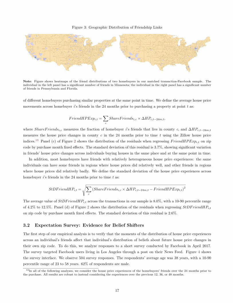
Figure 3: Geographic Distribution of Friendship Links

Note: Figure shows heatmaps of the friend distributions of two homebuyers in our matched transaction-Facebook sample. Theindividual in the left panel has a significant number of friends in Minnesota; the individual in the right panel has a significant numberof friends in Pennsylvania and Florida.

of different homebuyers purchasing similar properties at the same point in time. We define the average house pricemovements across homebuyer i’s friends in the 24 months prior to purchasing a property at point t as:

FriendHPExpi,t =∑c

ShareFriendsi,c ×∆HPc,t−24m,t,

where ShareFriendsi,c measures the fraction of homebuyer i’s friends that live in county c, and ∆HPc,t−24m,t

measures the house price changes in county c in the 24 months prior to time t using the Zillow house priceindices.13 Panel (c) of Figure 2 shows the distribution of the residuals when regressing FriendHPExpi,t on zipcode by purchase month fixed effects. The standard deviation of this residual is 3.7%, showing significant variationin friends’ house price changes across individuals buying houses in the same place and at the same point in time.

In addition, most homebuyers have friends with relatively heterogeneous house price experiences: the sameindividuals can have some friends in regions where house prices did relatively well, and other friends in regionswhere house prices did relatively badly. We define the standard deviation of the house price experiences acrosshomebuyer i’s friends in the 24 months prior to time t as:

StDFriendHPi,t =√∑

c

(ShareFriendsi,c ×∆HPc,t−24m,t − FriendHPExpi,t)2

The average value of StDFriendHPi,t across the transactions in our sample is 8.0%, with a 10-90 percentile rangeof 4.2% to 12.5%. Panel (d) of Figure 2 shows the distribution of the residuals when regressing StDFriendHPi,ton zip code by purchase month fixed effects. The standard deviation of this residual is 2.6%.

3.2 Expectation Survey: Evidence for Belief Shifters

The first step of our empirical analysis is to verify that the moments of the distribution of house price experiencesacross an individual’s friends affect that individual’s distribution of beliefs about future house price changes intheir own zip code. To do this, we analyze responses to a short survey conducted by Facebook in April 2017.The survey targeted Facebook users living in Los Angeles through a post on their News Feed. Figure 4 showsthe survey interface. We observe 504 survey responses. The respondents’ average age was 38 years, with a 10-90percentile range of 23 to 58 years. 62% of respondents are male.

13In all of the following analyses, we consider the house price experiences of the homebuyers’ friends over the 24 months prior tothe purchase. All results are robust to instead considering the experiences over the previous 12, 36, or 48 months.

17

Figure 4: Survey Interface

Note: Figure shows the interface in a user’s News Feed of the expectation survey conducted by Facebook on April 2017.

The first survey question elicits how often individuals talk to their friends about whether buying a house is agood investment. Regular conversations with friends about housing investments are important in order for thereto be a channel through which the house price experiences of friends can influence an individual’s own house pricebeliefs. Panel (a) of Figure 5 shows the distribution of responses to this question. About 43% of respondents gavethe modal answer, “sometimes.” The other possible responses were “never” (16% of responses), “rarely” (21% ofresponses), and “often” (20% of responses).

To measure an individual’s beliefs about future house price changes, we use the responses to the second question,which asked individuals to assign probabilities to various scenarios of house price growth in their zip codes over thefollowing 12 months. The survey enforced that the assigned probabilities add up to 100%. We use the responsesto determine the mean and standard deviation of the distribution of individuals’ house price beliefs.14 Panels (b)and (c) of Figure 5 show the distribution of these moments across the survey respondents. There is substantialdisagreement about expected house price growth among individuals living in the same local housing markets: whilethe median person expects house prices to increase by 5.3% over the next year, the 10-90 percentile range for thisestimate is 0.8% to 10.0%, and the standard deviation is 3.8%.

As a first test for whether individuals provide sensible and consistent responses to the expectation survey, Panel14To do this, we take the mid-point of each bucket, as well as the probabilities that individual respondents assign to that bucket.

For the open-ended buckets “Increase by more than 12%” and “Decrease by more than 8%”, we use point-estimates of 14% and -10%,respectively, but our results are robust to using different values assigned to these buckets. The roughly 15% of respondents who onlyassign probabilities to one bucket are assigned a standard deviation of beliefs of 0%.

18

Figure 5: Summary Statistics - Survey Responses

(a) Response to Question 10

.1.2

.3.4

Sha

re o

f Res

pons

es

Often Sometimes Rarely Never

How often do you talk to your friends aboutwhether buying a house is a good investment?

(b) Mean of House Price Expectations (Q2)

0.0

5.1

.15

Den

sity

-10 -5 0 5 10 15Mean of House Price Expectation (%)

(c) Standard Deviation of House Price Expectations (Q2)

0.0

5.1

.15

.2.2

5D

ensi

ty

0 2 4 6 8 10Standard Deviation of House Price Expectation (%)

(d) Mean of House Price Expectations by Response to Q3

0.0

5.1

.15

.2.2

5D

ensi

ty

-10 -5 0 5 10 15Mean of House Price Expectation (%)

Decrease About the Same Increase

Note: Figure shows summary statistics on the responses to the housing expectation survey. Panel (a) shows the responses to Question1. Panels (b) and (c) show the distribution of the mean and standard deviation of the belief distributions derived from individuals’answers to Question 2. Panel (d) shows the distributions of the mean of the belief separately by individuals’ answers to Question 3.

(d) of Figure 5 shows the distribution of the means of the belief distributions for individuals separately by theirresponses to Question 3, which asks if the respondents expect the average home price in their zip code to increase,stay the same, or decrease over the next 12 months. As a response to that question, 79.8% of individuals said theyexpected house prices in their zip code to increase over the next 12 months, 14.6% said they would expect themto stay about the same, and 5.6% expected them to decline (as a reference point, in the 12 months running up tothe survey, Los Angeles house prices increased by 7.4%). Individuals that thought it was most likely that houseprices in their zip code would increase over the next twelve months had a median belief about house price growthof 6.0%; the median expected house price growth of respondents who said house prices would stay about the same(decline) was 2.0% (-2.4%). While there are a small number of individuals who indicate they expect house priceto fall, yet assign probabilities that imply increasing house prices, the combined evidence documents a substantialdegree of consistency across individuals’ answers within the same survey.

We next analyze how moments of the distribution of house price changes across individual i’s social network inthe 24 months prior to answering the survey affect the corresponding moments of the distribution of beliefs aboutfuture house price changes. There is significant variation across respondents in both the mean and the standard

19

Table 2: Regression Results - House Price Expectations

(1) (2) (3) (4) (5) (6)

Δ Friends' House Prices (24m)

Out-of-CZ Friends - Mean 0.186**

(0.082)

Out-of-CZ Friends - St. D. 0.121**

(0.058)

All Friends - Mean 0.326** 0.322** -0.024

(0.144) (0.148) (0.055)

All Friends - St. D. 0.027 0.182** 0.184**

(0.145) (0.089) (0.090)

Zip FE and Demographic Controls Y Y Y Y Y Y

Specification Notes OLS IV IV OLS IV IV

N 426 426 426 426 426 426

Dep. Var.: Mean of Belief Distribution Dep. Var.: Standard Deviation of Belief Distribution

Note: Table analyzes the determinants of individuals’ expectations about house price changes in their own zip codes over the next12 months. In columns 1 to 3, the dependent variable is the mean of individuals’ belief distributions, based on their responses toQuestion 2 of the expectation survey (see Figure 4); in columns 4 to 6, the dependent variable is the standard deviation of these beliefdistributions. All specifications include fixed effects for the zip code of the survey respondents; we also control flexibly for age, gender,and the number of friends. Columns 1 and 4 present OLS specifications, while columns 2, 3, 5, and 6 present instrumental variablesregressions, where the moments of the house price experiences across an individual’s friends are instrumented for by the correspondingmoments of the distribution of experiences across their out-of-commuting zone friends. Standard errors are in parentheses. SignificanceLevels: * (p<0.10), ** (p<0.05), *** (p<0.01).

deviation of the experiences of their friends: indeed, FriendHPExpi,Apr17 has a mean of 15.1% and a standarddeviation of 1.7% across survey respondents. When measured only among out-of-commuting zone friends, it hasa mean of 16.3% and a standard deviation of 2.6%. Similarly, StDFriendHPi,Apr17 has a mean of 5.0% and astandard deviation of 1.7% across all friends of the survey respondents; among all out-of-commuting zone friends,the mean and standard deviation of StDFriendHPi,Apr17 are 6.9% and 1.7%, respectively.

Table 2 shows results from regressions of moments of the elicited belief distribution on moments of theexperience distribution among survey respondents’ friends. All specifications control for zip code fixed effects toensure that we are comparing individuals’ assessments of the same local housing markets; it also includes flexiblecontrols for the age, gender, and the number of friends of the respondent. In columns 1 to 3, the dependentvariable is the mean of the elicited belief distribution. Since all friends in Los Angeles experience the same recenthouse price changes, across-individual variation in friends’ house price experiences is driven by differences in theexperiences of their out-of-commuting zone friends as well as differences in the share of friends that live locally.As we discuss below, we want to isolate variation in friends’ experiences coming from the experiences of theirout-of-commuting zone friends, since this allows us to address a number of potential alternative interpretationsof our findings. Column 1 of Table 2 shows that a one-percentage-point (0.38 standard deviation) increase inthe average house price experience of an individual’s out-of-commuting zone friends, FriendHPExpOut−CZi,Apr17 , isassociated with a 0.19 percentage point (0.05 standard deviation) increase in the expected house price growthover the next year.15 In column 2, the main explanatory variable is the average house price experience of all

15The effect of FriendHPExpOut−CZi,Apr17 on the R-squared is relatively modest: conditional on the control variables, the house priceexperiences of an individual’s out-of-commuting zone friends explain an additional 1.1% - 1.6% of the observed variation in the meanof house price beliefs. Specifically, the OLS regression without controlling for out-of-commuting zone friends’ average house priceexperiences, but including all the other control variables, has an R-squared of 0.362; the within-zip code R-squared is 0.074. Whenwe include the out-of-commuting zone friends’ house price experiences as an additional control variable, the R-squared increases to0.373, and the within-zip code R-squared increases to 0.090. However, given the large sample sizes in the leverage choice regressions inSections 3.3 and 3.4, the belief shifter has sufficient power to identify statistically significant effects of beliefs on leverage. The numberof observations in Table 2 is lower than the total number of responses we observe. This is because 78 responses are from individualswho are the only respondents from their own zip code. Their responses are thus fully explained by the zip code fixed effects.

20

friends, FriendHPExpi,Apr17, instrumented for by the average house price experiences of the individuals’ out-of-commuting zone friends, FriendHPExpOut−CZi,Apr17 . This specification mirrors our baseline regressions in Sections3.3 and 3.4 below, and will allow us to compare estimates across specifications with different outcome variables. Aone-percentage-point increase in the house price experiences of all friends in the previous two years is associatedwith a 0.33 percentage point increase in individuals’ mean belief about house price growth over the comingyear. In column 3, we also include the standard deviation of house price experiences across individuals’ friends,StDFriendHPi,Apr17, instrumented by its out-of-commuting zone counterpart, as an additional control variable;it has no statistically significant effect on individuals’ average house price expectations.

The dependent variable in columns 4 to 6 of Table 2 is the standard deviation of the distribution of individuals’beliefs about future house price changes. Column 4 shows that a one-percentage-point (0.38 standard deviation)increase in StDFriendHPOut−CZi,Apr17 is associated with a 0.12 percentage point (0.08 standard deviation) increasein the standard deviation of the belief distribution. In column 5, the main explanatory variable of interest isthe standard deviation of house price experiences across all friends, instrumented for by its counterpart amongout-of-commuting zone friends. The estimated effect of a one-percentage-point increase in StDFriendHPi,Apr17

on the standard deviation of the belief distribution is 0.18 percentage points. In column 6, we also includeFriendHPExpi,Apr17 as a control variable, but it has no statistically significant effect on the standard deviationof the belief distribution.

Overall, these findings confirm that the mean and standard deviation of the house price experiences across anindividual’s friends can shift the corresponding moments of the distribution of that individual’s house price beliefs.In the following section we will use this insight to analyze the effect of house price beliefs on mortgage leveragechoice.

3.3 Main Results

We next test how moments of the distribution of house price experiences across a homebuyer’s friends affect thathomebuyer’s leverage choice in the sample of transactions described in Section 3.1. Based on the evidence inSection 3.2, we argue that these house price experiences provide shifters of individuals’ distributions of beliefsabout future house price changes. We will also argue below that friends’ house price experiences are orthogonalto other factors that might influence a homebuyer’s leverage choice.

In our baseline regression specification R1, the unit of observation is a housing transaction. We regress thecombined loan-to-value (CLTV) ratio for transaction i at time t in county c and financed by mortgage lender l onmoments of the distribution of the house price experiences of the homebuyer’s friends. This combined loan-to-valueratio includes all mortgages originated to finance the home purchase. We also control for a rich set of homebuyercharacteristics,16 and include county by purchase month by lender fixed effects, ψt,c,l.17 This allows us to comparethe leverage choices across individuals who borrow from the same lender in the same county and at the same pointin time, and who therefore faced the same schedule of loan-to-value ratios and interest rates to choose from.

CLTVi,t,c,l = α+ β1MeanFriendHPi,t + β2StDFriendHPi,t + β3Xi,t + ψt,c,l + εi,t,z, (R1)16With the exception of age, which can be observed at the point of the transaction, other homebuyer characteristics are observed

as of the points of the InfoBase snapshots. We assign the value from the most proximate snapshot. We flexibly control for homebuyerincome, age, household size, family status, occupation, and education level. We also control for the number of friends, the number ofout-of-commuting zone friends, and the number of counties in which an individual has friends.

17Even though Hurst et al. (2016) have shown that most lenders do not vary their mortgage pricing geographically, this choice offixed effects is conservative, and ensures that we are comparing the leverage choices of individuals facing the same trade-offs betweenmaking a smaller downpayment and paying higher interest rates. In the rare cases where the first and second mortgages are by differentlenders, we use the identity of the lender of the first mortgage to determine the lender fixed effect.

21

In order to use estimates of β1 and β2 to learn about the relationship between beliefs and leverage, we needto ensure that our key explanatory variables, MeanFriendHP and StDFriendHP , only affect leverage choicethrough their effect on homebuyers’ beliefs about the distribution of future house price changes. A first concern isthat individuals who have more local friends, and for whom higher local house prices would thus lead to a higherMeanFriendHP , might also be more affected by this local house price growth through channels other than theeffect on their house price expectations. For example, if individuals with more local friends were more likely to ownlocal property, then they would be more likely to benefit from higher capital gains, allowing them to make a largerdownpayment on any subsequent property purchase. To rule out confounding effects through such alternativechannels, we estimate regression R1 using an instrumental variables (IV) strategy, where we instrument for themean and standard deviation of all friends’ house price experiences with the mean and standard deviation of thehouse price experiences of out-of-commuting zone friends (see also the discussion in Section 3.2).18

Testing Baseline Predictions. Table 3 shows the results from regression R1. The baseline estimate incolumn 1, which does not control for homebuyer demographics, suggests that individuals whose friends experienceda one-percentage-point higher house price appreciation over the past 24 months increase their downpayments (andreduce their CLTV ratios) by between 8 and 9 basis points. A one within-zip-code-month standard deviationincrease in the house price appreciation experienced by an individual’s friends is thus associated with that individualmaking a 31 basis points larger downpayment. This finding suggests that individuals’ house size choice is relativelyinsensitive to the perceived collateral return, and that these individuals thus behave more like in the fixed housesize scenario than in the variable house size scenario.19 Column 1 also shows that individuals whose friends hadmore dispersed house price experiences, and who thus expected more variance in future house price changes, chosehigher leverage: a one-percentage-point increase in the across-friends standard deviation of house price experiencesover the past 24 months is associated with a 35 basis points increase in the combined loan-to-value ratio. Thisresult is also consistent with the predictions from the fixed house size scenario: individuals that expect futurehouse price growth to be more dispersed perceive large house price drops to be more likely. This increases thebenefits of not putting all their savings into the house, and therefore increases their optimal leverage choice.

In column 2 of Table 3, we also control flexibly for a large number of homebuyer characteristics. The estimatedeffects of the house price experiences of a person’s friends is remarkably stable with respect to the addition of theseobservable controls. This provides additional evidence consistent with Bailey et al. (2017) that the house priceexperiences of a person’s friends in a given year are uncorrelated with that person’s observable characteristics,and reduces concerns that the results are driven by selection on unobservable buyer characteristics (see Altonji,Elder and Taber, 2005). In column 3, we interact the buyer demographics with year fixed effects. This allows,for example, the effect of having a different education or a different profession on leverage choice to vary byyear. This specification provides a first test of whether our findings could be explained by correlated shocks tohomebuyers and their friends. For example, one might have worried that less-educated Los Angeles residents havemore friends in regions with a relatively less-educated population. In that case, a positive shock to the incomeprospects of less-educated individuals in a given year might both raise house prices where less-educated buyershave friends, and would increase the ability of these less-educated buyers to make larger downpayments. Our

18The instrument has an F-Statistic above 1,500 across all specifications, largely driven by the fact that the set of out-of-commutingzone friends, which is used to construct the instruments, is a subset of the set of all friends, which is used to construct the instrumentedvariables, MeanFriendHPi,t and StDFriendHPi,t.

19This does not mean that more pessimistic individuals did not also reduce their housing market investments, as in the polarcase with no collateral return sensitivity that we study in Section 1 above. Indeed, Bailey et al. (2017) document that individualswhose friends experienced lower recent house price growth did buy smaller houses: a one-percentage-point smaller friends’ house priceexperience was associated with purchasing a 0.3 percentage points smaller property. Instead, the estimate in column 1 of Table 3suggests that as individuals got more pessimistic, their desire to reduce their financial exposure to potential house price declinesincreased faster than the reduction in that exposure that was possible to achieve by buying a smaller house. As a result, they endedup buying (slightly) smaller houses with larger overall leverage (see also the simulations of the more general model in Appendix B).

22

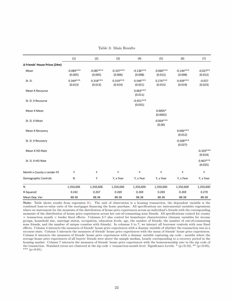
Table 3: Main Results

(1) (2) (3) (4) (5) (6) (7)

Δ Friends' House Prices (24m)

Mean -0.084*** -0.087*** -0.107*** -0.136*** -0.060*** -0.144*** -0.027**

(0.005) (0.005) (0.006) (0.008) (0.012) (0.008) (0.012)

St. D. 0.349*** 0.318*** 0.319*** 0.546*** 0.276*** 0.439*** -0.027

(0.013) (0.013) (0.014) (0.021) (0.015) (0.019) (0.023)

Mean X Recourse 0.063***

(0.011)

St. D. X Recourse -0.451***

(0.031)

Mean X Mean 0.0005*

(0.0002)

St. D. X Mean -0.004***

(0.00)

Mean X Recovery 0.046***

(0.012)

St. D. X Recovery -0.268***

(0.027)

Mean X HO-Rate -0.103***

(0.014)

St. D. X HO-Rate 0.463***

(0.025)

Month x County x Lender FE Y Y Y Y Y Y Y

Demographic Controls N Y Y, x Year Y, x Year Y, x Year Y, x Year Y, x Year

N 1,350,606 1,350,606 1,350,600 1,350,600 1,350,600 1,350,600 1,350,600

R-Squared 0.242 0.267 0.269 0.269 0.269 0.269 0.270

Mean Dep. Var. 88.38 88.38 88.38 88.38 88.38 88.38 88.38

Note: Table shows results from regression R1. The unit of observation is a housing transaction, the dependent variable is thecombined loan-to-value ratio of the mortgages financing the home purchase. All specifications are instrumental variables regressionswhere we instrument for the moments of the distribution of house price experiences across an individual’s friends with the correspondingmoments of the distribution of house price experiences across her out-of-commuting zone friends. All specifications control for county× transaction month × lender fixed effects. Columns 2-7 also control for homebuyer characteristics (dummy variables for incomegroups, household size, marriage status, occupation, education levels, age, the number of friends, the number of out-of-commutingzone friends, and the number of unique counties with friends). In columns 3 to 7, we interact all borrower controls with year fixedeffects. Column 4 interacts the measures of friends’ house price experiences with a dummy variable of whether the transaction was in arecourse state. Column 5 interacts the measures of friends’ house price experiences with the mean of friends’ house price experiences.Column 6 interacts the measures of friends’ house price experiences with a dummy variable capturing zip code - months where theaverage house price experiences of all buyers’ friends were above the sample median, loosely corresponding to a recovery period in thehousing market. Column 7 interacts the measures of friends’ house price experiences with the homeownership rate in the zip code ofthe transaction. Standard errors are clustered at the zip code × transaction-month level. Significance Levels: * (p<0.10), ** (p<0.05),*** (p<0.01).

23

results are essentially unchanged from our baseline specification, suggesting that such correlated shocks are not akey driver of our results. We provide a large number of additional robustness checks in Section 3.4.

How should one think about the magnitude of these baseline estimates? One option is to use a split-sampleIV approach to combine our estimates from column 3 of Table 3 with the estimates from the survey analyzed inSection 3.2. This approach would suggest that individuals who expect a one-percentage-point lower house pricegrowth over the coming twelve months would choose a 0.107

0.326 = 33 basis points lower downpayment. Similarly,one-percentage-point increase in the expected standard deviation of house price growth over the next twelvemonths would be associated with a 0.319

0.182 = 175 basis points lower downpayment.20 To judge the plausibility ofthese magnitudes, it is important to recall that the survey elicits beliefs about house price growth over the comingtwelve months, while mortgage leverage choices are affected by individuals’ belief distribution about the cumulativehouse price growth over the expected life-time of the mortgage.21 Translating the responses to the expectationssurvey into such cumulative house price changes requires making assumptions on both the time-series propertiesof the house price growth process as well as the relevant time horizon considered by households when deciding ontheir mortgage leverage. For example, in Appendix A.4 we show that under a standard AR(1) process for houseprice changes, with an annual persistence of 0.65 as estimated by Guren (2018), a one-percentage-point increasein the standard deviation of house price changes over the next year translates into a 4.5 percentage point increasein the cumulative standard deviation over the next five years, and an almost 8 percentage point increase in thecumulative standard deviation over the next ten years. When compared against an 8 percentage point increasein the standard deviation of cumulative house price changes over the lifetime of the mortgage, an adjustment ofleverage of 175 basis points appears much more reasonable than when compared against a one percentage pointincrease in the standard deviation of house price changes over the next year.

Testing Additional Predictions. Columns 1 to 3 of Table 3 documented a relationship between beliefsand leverage choices most consistent with the fixed house size scenario. Columns 4 to 6 verify the additionalpredictions from Section 2.2, which establishes that in the fixed house size scenario, the relationship betweenbeliefs and leverage should be stronger when default is relatively more likely.

Column 4 tests Proposition 2a, which highlights that the downpayment protection force at the heart of thefixed house size scenario should be particularly strong when the cost of mortgage default is low, and default istherefore relatively more likely. We proxy for the cost of default by whether or not the transaction occurred in arecourse state. In recourse states, lenders can collect on debt not covered by the sale of a foreclosed property bygoing after other assets of the defaulting borrowers. This substantially increases the cost of default for borrowersin recourse states.22 About half of our transactions come from recourse states. Consistent with Proposition 2a forthe fixed house size scenario, the effect of friends’ average house price experiences on individuals’ leverage choicesis about twice as large for transactions in non-recourse states. Similarly, the effect of a higher standard deviationof friends’ house price experiences on mortgage leverage choices is over five times as large in non-recourse statesas it is in recourse states. This highlights that the downpayment protection force, which is central to the fixedhouse size scenario, is indeed stronger in legal environments that feature relatively low costs of default.

Columns 5 and 6 of Table 3 test Proposition 2b from Section 2.2, which highlights that, in the fixed house size20These estimates are obtained by using the point estimates from Table 2 (columns 2 and 5) in the denominator. However, given

the relatively large standard errors around these estimates, there is also significant uncertainty around these split-sample IV results.21For buyers of single-family residences, the median expected duration of staying in the home is in excess of 10 years.22Ghent and Kudlyak (2011) analyze mortgage default behavior across U.S. states, and find strong evidence that the recourse/non-

recourse environment does indeed have significant effects on the default behavior of borrowers, as would be predicted if it inducedsignificant differences in the costs of default. Specifically, the authors find that at the average value of negative equity, the monthlyprobability of default is 1.3 times higher in non-recourse states than it is in recourse states. All else equal, this means that it takes8.6% more negative equity to make the probability of default in a recourse state the same as the probability of default in a non-recoursestate. See also the discussion in Kuchler and Stroebel (2009).

24

scenario, the effects of changes in house price beliefs on leverage choice should be smaller if the baseline houseprice belief is more optimistic, and the default option is thus less important. Column 5 conducts a cross-sectionaltest, and interacts our belief shifters with the mean of friends’ house price experiences. Changes in both the meanand the variance of friends’ house price experiences indeed have smaller effects for individuals who are alreadystarting from a higher mean house price expectation, and who thus perceive a lower likelihood of default. Column6 conducts a time-series text, and interacts the mean and standard deviation of friends’ house price experienceswith a dummy variable that captures whether or not the average house price experience of all buyers in thepurchase zip code-month was above the sample median value. For these transactions, we expect the homebuyersto be relatively more optimistic about future house price changes, and to therefore perceive a lower probability ofdefault (see Case, Shiller and Thompson, 2012, and Kuchler and Zafar, 2015, for evidence on such extrapolativehouse price expectations). Consistent with the predictions from the fixed house size scenario, the effects of boththe mean and standard deviation of friends’ house price experiences on leverage choices are significantly larger inabsolute terms during the housing bust period than they are during the recovery period.23 This is consistent withthe downpayment protection force being stronger during periods with a higher perceived likelihood of default.

In column 7, we interact the mean and standard deviation of the house price experiences of homebuyers’ friendswith the homeownership rate in the zip code of the transaction. The homeownership rate is a proxy for the extentto which individuals’ home purchase decisions are sensitive to expected house price changes. In markets withhigh homeownership rates, pessimistic individuals wanting to live in a certain zip code (for example, because ofproximity to work or good schools) are less likely to find a suitable rental property as a way of reducing theirhousing market exposure. Such high-homeownership-rate zip codes are thus a better approximation of the fixedhouse size scenario, in which reductions in downpayments provide a relatively easier way for households to reducetheir housing market exposure. Consistent with this, the estimates show that in regions with high homeownershiprates, we see a larger effects of changes in the perceived default probability on leverage choices.

Taken together, the behavior of the homebuyers in our sample corresponds to the predictions from the fixedhouse size scenario, in which relatively pessimistic homebuyers do not end up renting or purchasing substantiallycheaper homes.24 These pessimistic homebuyers therefore make smaller downpayments in order to reduce theirhousing market exposures, in particular in states where the cost of default is comparatively smaller, and duringtime periods when there are concerns about substantial price drops in the housing market.

3.4 Robustness Checks and Ruling Out Alternative Explanations

Our interpretation of the results in Section 3.3 is that the relationship between friends’ house price experiences andleverage was driven by the effects of friends’ experiences on an individual’s belief about future house price growth.In this section, we rule out a number of alternative interpretations of the correlation between friends’ house priceexperiences and individuals’ mortgage leverage choice. As we address these alternative interpretations, we notethat most of these stories could have potentially explained the effect of friends’ average house price experienceson leverage. However, the effect of the dispersion of friends’ house price experiences on leverage choices are muchharder to rationalize with alternative mechanisms, as are the differential effects across recourse/non-recourse states,

23A potential concern when interpreting these differential effects across time comes from the fact that we only observe the friendshipnetwork at one point in time, July 2015. This network becomes a noisier measure of individuals’ contemporaneous network thefurther back we go, which could induce increased attenuation bias for measuring friends’ house price experiences for buyers in earliertransactions. However, given that the housing bust period preceded the housing recovery period, such an attenuation bias wouldreduce the measured effect during the housing bust period, and therefore work against producing the effect that we uncover.

24One caveat regarding the generalizability of these findings is that our sample is restricted to purchases by owner-occupiers, sincewe cannot match buyers making investment purchases to their respective Facebook accounts. While we do not have the data to analyzethe leverage choices of these investment buyers, our theoretical framework suggests that those individuals’ collateral decisions shouldbe more return sensitive. They might therefore respond to increasing optimism by buying more houses with higher leverage.

25

across periods with relatively high/low average beliefs, and across regions with different homeownership rates.A first concern we address is that the instruments in our baseline regression, the moments of the house price

experiences of out-of-commuting zone friends, might still be correlated with the individuals’ own house priceexperiences, and therefore potentially with their own capital gains, in particular for individuals who have morefriends in close-by commuting zones that have house price movements similar to those in their own commutingzone. In column 1 of Table 4, we therefore use moments of the house price experiences of out-of-state friends asinstruments. Reassuringly, the magnitudes of the effects in this specification are, if anything, slightly larger thanin our baseline specifications.

In column 2 of Table 4, we restrict the sample to purchases by individuals with more than 50 out-of-commutingzone friends; in column 3, we restrict the sample to transactions by individuals with friends in at least 35 counties.These specifications address concerns that the effects of the dispersion of friends’ experiences on leverage could bedriven by individuals without sufficiently many geographically distant friends to construct powerful shifters of thebelief distribution. The magnitude of the estimates are very similar to those in the baseline specification.

Table 4: Robustness Checks I

(1) (2) (3) (4) (5) (6) (7)

Δ Friends' House Prices (24m)

Mean -0.112*** -0.094*** -0.093*** -0.080*** -0.090*** -0.084*** -0.114***

(0.007) (0.006) (0.007) (0.007) (0.025) (0.006) (0.008)

St. D. 0.456*** 0.283*** 0.278*** 0.319*** 0.256*** 0.273*** 0.370***

(0.019) (0.016) (0.017) (0.014) (0.065) (0.014) (0.023)

Δ Friends' County Income (24m)

Mean -8.015***

(0.962)

St. D. -13.33***

(0.910)

Friends' Foreclosure Rate (24m)

Mean 40.83***

(1.773)

St. D. -32.37***

(3.479)

Month x County x Lender FE Y Y Y Y Y Y Y

Demographic Controls Y, x Year Y, x Year Y, x Year Y, x Year Y, x Year Y, x Year Y, x Year

Specification Notes

Out-of-State

Friends' Exp.

As Instrument

> 50 Out-Of-

Commuting

Zone Friends

> 35 Unique

Counties

Geographically

Non-Clustered

Profession

Only Friends in

Recourse States

N 1,350,348 996,864 937,075 1,253,013 1,308,731 1,347,592 1,349,396

R-Squared 0.268 0.271 0.280 0.269 0.277 0.270 0.269

Mean Dep. Var. 88.38 88.65 88.86 88.39 88.37 88.38 88.38

Note: Table provides robustness checks to the baseline results presented in Table 3. The unit of observation is a home transaction,the dependent variable is the combined loan-to-value ratio in the transaction. All specifications include controls and fixed effects asin column 3 of Table 3. In column 1, we instrument for moments of the house price experiences of the buyers’ total friends withthe corresponding moments of the distribution of house price experiences of the buyers’ out-of-state friends. In column 2, we restrictthe sample to purchases by individuals with at least 50 out-of-commuting zone friends, in column 3 to purchases by individuals withfriends in at least 35 unique counties. Column 4 also controls for the average income changes in the counties where an individualhas friends. In column 5, we focus on purchases by individuals working in geographically non-clustered professions (e.g., teachers andlawyers). Column 6 also controls for the average foreclosure rate in the counties where an individual has friends. Column 7 only usesthe house price experiences of out-of-commuting zone friends in recourse states to instrument for the house price experiences of allfriends. Standard errors are clustered at the zip code × transaction-month level. Significance Levels: * (p<0.10), ** (p<0.05), ***(p<0.01).

A further possible concern is that unobserved shocks to an individual’s ability to make a downpayment ina given year might be correlated with her friends’ house price experiences in that year. Such an alternativeinterpretation requires a shock to an individual’s wealth or income that contemporaneously moves house pricesin geographically distant regions where she has friends. As discussed above, our baseline regressions alreadyminimize the scope for such potentially confounding effects, by including year-specific controls for a large number

26

of observable characteristics of homebuyers. We next address the one additional potential confounder that we wereable to identify. In particular, many people have friends that work in the same sector of the economy. If economicactivity in that sector features significant geographic clustering (e.g., tech in Silicon Valley), positive shocks tothat sector in a given year might both enable an individual to make a larger downpayment and drive up aggregatehouse prices in those sector-exposed regions where the individual has friends.

To rule out this explanation of our findings, column 4 includes the average income change in the county wherethe person has friends as a control, in addition to the average house price change. We measure income annuallyusing data from the Tax Statistics of Income (SOI). In addition, column 5 restricts the sample of transactions tothose in which the homebuyer works in geographically non-clustered professions (e.g., lawyers and teachers). Anypositive shocks to such professions, which might increase those individuals’ ability to make a larger downpayment,should not affect house prices in regions where they have friends. This is because there are no parts of the U.S.where there are so many teachers or lawyers that positive shocks to those professions can shift aggregate houseprices. In both specifications the estimates are similar to our baseline estimates, suggesting that common shocksto individuals and their friends that shift house prices in areas where their friends live cannot explain our findings.

A further potential alternative interpretation of our findings is that when house prices decline in counties wherean individual has friends, and there are subsequently more foreclosures in those counties, individuals might updateboth their own house price beliefs as well as their expectations about the cost of default or the benefits of theforeclosure process, both of which might also directly affect their leverage choice. To address such concerns, column6 also includes measures of the share of all properties in friends’ counties that experienced a foreclosure over theprevious 24 months, based on data provided by Zillow. While a higher foreclosure rate in friends’ locations isassociated with larger leverage and a smaller downpayment, the inclusion of this additional control variable doesnot significantly affect the estimated effect of friends’ house price experiences on mortgage leverage choice.25 Incolumn 7, we only use the house price experiences of friends in recourse states to instrument for the house priceexperiences of all friends. If most of the effect came through individuals learning about the cost of default whenhouse prices fall where their friends live, then the estimated effect should be smaller when only using variation inhouse prices in recourse states where a given house price change translate into fewer foreclosures. However, theestimated coefficients are, in fact, almost identical in size to our baseline estimates.

An additional set of potential alternative interpretations for our results comes from constraints on individuals’ability to freely choose their mortgage amount. In particular, imagine that mortgage amounts cannot be increaseddue to constraints outside of the model. More optimistic individuals would still desire to purchase a larger ormore expensive home. As a result, any increase in the value of the property these optimistic individuals purchasewill automatically lead to a lower LTV ratio (they increase the “value” without being able to change the “loan”part). However, this decline in the LTV ratios of optimistic individuals would not be due to optimistic borrowersoptimally choosing lower LTV ratios (as is the case in the story we tell in the paper), but because of the constraintson their ability to increase their mortgage amount.

We have identified three possible sources of such constraints on borrowers’ ability to increase the size of theirmortgage, and have verified that these constraints are unlikely to explain our findings. The first possible constraintcomes from potentially binding debt-to-income (DTI) or payment-to-income ratios, since banks usually requireindividual mortgage holders to have sufficient income to afford their monthly mortgage payments. To test whetherour estimates are the results of such constraints preventing optimistic borrowers from further increasing their

25While the house price experiences and foreclosure rates across friends’ counties are naturally correlated, they are far from collinear.Specifically, the extent to which declining house prices translate into more foreclosures depends both on the legal environment acrossstates as well as on the initial level of equity that individuals have in their homes, which, in turn, depends on the entire house pricehistory in the county. In addition, there is a substantial time-lag between the initial house price decline and default/foreclosure activity.

27

mortgage amounts, column 1 of Table 5 shows our baseline estimates restricted to a sample of individuals with aDTI ratio below the median value of three.26 The estimates in this sample are similar to those in the full sample,suggesting that binding DTI ratios cannot explain our findings.

Table 5: Robustness Checks II

(1) (2) (3) (4) (5) (6)

Δ Friends' House Prices (24m)

Mean -0.089*** -0.106*** -0.100*** -0.099*** -0.105*** -0.094***

(0.009) (0.006) (0.006) (0.006) (0.009) (0.007)

St. D. 0.248*** 0.326*** 0.304*** 0.306*** 0.258*** 0.324***

(0.022) (0.014) (0.014) (0.013) (0.021) (0.014)

Overpay -0.067***

(0.001)

Month x County x Lender FE Y Y Y Y Y Y

Demographic Controls Y, x Year Y, x Year Y, x Year Y, x Year Y, x Year Y, x Year

Specification Notes DTI < MedianMortgage <

(CLL - $10k)

Counties with p75

house price below

CLL

"Overpay" < 0Transactions prior

to January 2013

N 588,358 1,206,593 1,246,448 1,334,769 602,461 1,064,658

R-Squared 0.313 0.285 0.265 0.282 0.300 0.265

Mean Dep. Var. 86.81 88.69 88.78 88.40 90.55 88.39

Note: Table provides robustness checks to the baseline results presented in Table 3. The unit of observation is a home transaction,the dependent variable is the combined loan-to-value ratio in the transaction. All specifications include controls and fixed effects asin column 3 of Table 3. In column 1, we restrict the sample to transactions with a debt-to-income (DTI) ratio below the samplemedian of 3. In column 2, we restrict the sample to transactions with a mortgage of at least $10,000 below the conforming loan limit(CLL). In column 3, we restrict the sample to transactions in counties where the 75th percentile of transaction prices was below theCLL. In column 4, we also control for “Overpay”, a variable that was constructed as the differences in the transaction price and ahedonic valuation of the property. In column 5, we restrict the sample to transactions with negative values of “Overpay”, where thetransaction price was below the property’s hedonic valuation. In column 6, we restrict the sample to transactions prior to January2013, a period with a negative correlation of county-level wealth and county-level house price changes. Standard errors are clusteredat the zip code × transaction-month level. Significance Levels: * (p<0.10), ** (p<0.05), *** (p<0.01).

Conforming loan limits might provide a second constraint on the ability of borrowers to increase their mortgageamounts. Indeed, during much of our sample period, obtaining a mortgage with an LTV ratio above 80% requiredgetting a conforming mortgage, which puts an upper bound on the size of the loan. Optimistic individuals whoare close to that upper bound would not be able to buy more expensive homes without also reducing their finalLTV ratios. To show that such constraints do not explain our results, column 2 of Table 5 focuses the sampleon individuals who take out a mortgage that is at least $10,000 lower than the conforming loan limit in theircounty, and who thus would have been able to further increase their LTV ratios if they had chosen to do so. Theestimates in this sample are very similar to those in the baseline sample, suggesting that our results are unlikely tobe driven by constraints coming from the conforming loan limit. In addition, in column 3 we repeat the analysisonly for counties where at least 75% of properties transact at values below the conforming loan limit, and wheresuch properties could thus have been purchased and fully financed with a conforming mortgage. In these counties,where few buyers are constrained by conforming loan limits, we see a similar relationship between house pricebeliefs and mortgage leverage choice as in the full sample, again confirming that constraints on borrowers’ abilityto increase their mortgage above the conforming loan limit cannot explain our findings.

A third constraint on an optimistic buyer’s ability to increase her mortgage could come from the assessedvalue of the property: banks might determine the allowable mortgage as a fraction of their own assessed property

26Our data do not include information on the monthly payments for each mortgage, so we cannot calculate the mortgages’ payment-to-income ratios. However, given the limited heterogeneity in interest rates, individuals with a below-median debt-to-income ratio areunlikely to be constrained by a payment-to-income ratio.

28

value (based, for example, on automated valuation models) instead of basing it on the transaction price. To theextent that more optimistic people end up paying more for otherwise identical properties, as suggested by Baileyet al. (2017), both optimistic and pessimistic people might end up with the same loan amount, but optimisticpeople would pay more for the same house, and would therefore have a lower observed LTV ratio. At firstsight, the potential for such a mechanism to drive our results seems limited, given the extensive evidence in theliterature that the vast majority of appraised property values are at or above the transaction price (e.g., Cho andMegbolugbe, 1996). We also show that, empirically, such constraints are unlikely to explain our results. To dothis, we construct a measure of “overpaying” for a property as the difference between the transaction price anda predicted property price based on a hedonic valuation model (see Appendix D.3 for details). We then includethat measure of overpaying as an additional regressor in column 4 of Table 5. The relationship between beliefsand leverage is unaffected by the addition of this further control variable. In column 5, we restrict the sample totransactions where the transaction price was below the predicted value from our hedonic valuation. In this sample,the effects of beliefs on leverage are very similar as in the full sample, providing further evidence that constraintsdue to assessed property values are unlikely to explain our findings.

An additional challenge to our interpretation comes from our inability to directly control for wealth in regressionR1. If wealthy individuals have friends in richer counties, and if these richer counties experienced higher house priceappreciation, then our estimates of β1 might just be picking up that wealthy people make larger downpayments.There are two reasons why we think that such a story is unlikely to explain our results. First, while we cannotcontrol for wealth directly, we do control for a number of demographic characteristics that are likely to be correlatedwith wealth, such as income and occupation. The fact that the addition of these control variables does not affectour estimates of β1 suggests that the coefficient is unlikely to pick up any demographic characteristics that correlatewith having friends in areas with higher house price growth (see columns 1 and 2 of Table 3). Second, there are nofixed demographic characteristics that are consistently correlated with having friends in areas with higher houseprice appreciation, since counties that experienced above-average house price appreciation in the beginning of oursample generally had below-average house price growth towards the end of our sample. Indeed, in the period priorto January 2013, richer counties actually experienced below-average house price changes (see Appendix D.4). Yet,column 6 of Table 5 shows that there remains a negative relationship between friends’ house price experiences andhomebuyers’ leverage choice during this period, suggesting that our inability to directly control for wealth doesnot explain our findings.

Wealth effects might also operate through a bequest channel that is not yet ruled out by the evidence presentedabove: if an individual has family members that live in those areas where she has friends, and if those familymembers own real estate, then house price increases in those areas might increase her expected bequest. Thiswealth channel could then provide an alternative explanation for why individuals make larger downpayments whentheir geographically distant friends have experienced higher house price increases. We rule out such an explanationin a number of ways. First, columns 1 to 6 of Table 6 separately explore the house price experiences across anindividual’s social network of work friends, family friends, and college friends. Since not all individuals reporttheir family member, their employer, or their college on Facebook, these regressions have fewer observations thanour baseline estimates. In columns 1, 3, and 5, we run our baseline regression (corresponding to column 3 of Table3), but only on the set of individuals for whom we can identify at least ten work friends, ten family friends, orten college friends, respectively. In columns 2, 4, and 6, we then run the same regression, but only use the houseprice experiences among out-of-commuting zone work friends, family friends, and college friends, respectively, toinstrument for all friends’ house price experiences.27 While one might expect to inherit a house from a family

27Bailey et al. (2017) documented that the average house price experiences across these three separate out-of-commuting zonenetworks are relatively uncorrelated. This suggests that homebuyers’ family friends do not, in general, live in the same parts of the

29

Table 6: Robustness Checks III

All Friends

(1) (2) (3) (4) (5) (6) (7)

Δ Friends' House Prices (24m)

Mean -0.126*** -0.191*** -0.121*** -0.133*** -0.089*** -0.086*** -0.362***

(0.014) (0.030) (0.012) (0.018) (0.017) (0.033) (0.027)

St. D. 0.366*** 0.629*** 0.254*** 0.333*** 0.222*** 0.118 0.776***

(0.035) (0.119) (0.029) (0.074) (0.039) (0.091) (0.051)

Month x County x Lender FE Y Y Y Y Y Y Y

Demographic Controls Y, x Year Y, x Year Y, x Year Y, x Year Y, x Year Y, x Year Y, x Year

Specification Notes All FriendsSame

EmployerAll Friends Same College All Friends Family

Purchase in Home

State, Out-of-State

Friends for Instrument

N 257,450 257,450 368,612 368,612 167,587 167,587 485,031

R-Squared 0.323 0.324 0.297 0.298 0.343 0.340 0.300

Mean Dep. Var. 89.72 89.70 88.22 88.20 91.11 91.10 88.96

Same Employer Same College Family

Note: Table provides robustness checks to the baseline results presented in Table 3. The unit of observation is a home transaction,the dependent variable is the combined loan-to-value ratio in the transaction. All specifications include controls and fixed effects asin column 3 of Table 3. In columns 1 and 2, we focus on purchases by people for whom we can identify at least ten work friends, incolumns 3 and 4 on purchases by people for whom we can identify at least ten college friends, and in columns 5 and 6 on purchasesby people for whom we can identify at least ten family members. In columns 1, 3, and 5, we repeat our baseline specification onthe restricted sample for comparability. In columns 2, 4, and 6, we use the house price experiences of an individual’s geographicallydistant work friends, college friends, and family members, respectively, to instrument the corresponding moments of the house priceexperiences among all friends. In column 7, we only include transactions of individuals who report a hometown, and who purchasea property in their home state. We use these buyers’ out-of-state friends’ house price experiences to instrument for the house priceexperiences of all friends. Standard errors are clustered at the zip code × transaction-month level. Significance Levels: * (p<0.10),** (p<0.05), *** (p<0.01).

member, this is much less likely for a colleague or college friend. Yet, our results are very similar when exploitingvariation in house price experiences across these three networks, suggesting that wealth effects are not a key driverof our findings. Finally, column 7 restricts the sample to individuals who report their hometown on Facebook, andwho purchase a property in their home state. We use the house price experiences of their out-of-state friends as aninstrument. For those individuals, the exposure of their expected bequest to out-of-state house price movementsis smaller, since the properties they might inherit are likely to be located in their home state. Yet, we find asomewhat larger correlation between the house price experiences of their geographically distant friends and theirleverage choices, providing additional evidence against important bequest effects.

A final concern with our interpretation comes from the fact that we focus on exploring the intensive marginchoices among homeowners. Bailey et al. (2017) show that more optimistic individuals are more likely to becomehomeowners, raising concerns that optimistic and pessimistic homeowners might differ on other characteristics thatcould affect their downpayment decisions. However, such a selection story would, if quantitatively important, pushagainst our findings. In particular, the selection story would suggest that pessimistic homebuyers obtain largernon-financial benefits from homeownership, for example because they purchase a home that is a great match withtheir consumption preferences. As a result, they would perceive defaulting and moving to be more costly. Thiswould reduce the strength of the downpayment protection force, and push more pessimistic individuals to makelarger downpayments, not smaller ones, as we see in the data.

country as their work or college friends.

30

4 Beliefs and Leverage Choice: Ancillary Evidence

The previous section documented that more optimistic individuals make larger downpayments, consistent with thedirectional predictions from the fixed house size scenario. In this section, we show that this relationship betweenhouse price beliefs and mortgage leverage choice is consistent with various additional survey data. We also provideadditional evidence for the importance of the downpayment protection force that is central to the predictions fromthe fixed house size scenario.

4.1 NY Fed Survey of Consumer Expectations.

We first analyze survey data from the 2014 Real Estate and Housing Module of the New York Fed Survey ofConsumer Expectations (SCE).28 Within these data, we consider the determinants of individuals’ (anticipated)leverage choices. Our key outcome variable is the answer to the following question asked of current homeowners:“What is the percent chance that over the next 12 months you will apply for an additional loan on your primaryresidence?” In Figure 6, we explore how the answer to this question differs with respondents’ expectations. In theleft panel, we sort respondents by their beliefs about house price growth in their neighborhood over the coming12 months, which was also elicited in the SCE. In the right panel, we sort respondents by their answer to thefollowing question: “What is the percent chance that over the next 12 months you will enter foreclosure or loseyour home through a repossession?”

Figure 6: Expectation of Applying for Additional Loan

02

46

8P

roba

bilit

y of

App

lyin

g fo

r Add

ition

al L

oan

(%)

<0% 0%-5% 5%-10% >10%

By Expected House Price Growth (12 months)Probability of Applying for Additional Loan (12 Months)

02

46

810

Pro

babi

lity

of A

pply

ing

for A

dditi

onal

Loa

n (%

)

0% 1%-10% >10%

By Expected Probability of Foreclosure (12 months)Probability of Applying for Additional Loan (12 Months)

Note: Figure shows summary statistics based on data from the FRBNY SCE. The left panel shows the average probability that surveyrespondents assign to applying for an additional loan on their property over the next 12 months, in percent, separately by groups ofexpected house price growth over the next 12 months. The right panel shows the average probability of applying for an additionalloan separately by the probability that individuals assign to having their house foreclosed over the next 12 months.

In both panels, there is evidence that individuals who are more pessimistic are more likely to want to increaseleverage, thereby reducing their financial exposure to the housing market. However, while these results are highlyconsistent with the downpayment protection force that is central to the predictions of the fixed house size scenario,there are other possible explanations for the observed correlations. For example, in regions where the economy is

28The Survey of Consumer Expectations is a monthly online survey of a rotating panel of nationally representative household headslaunched by the Federal Reserve Bank of New York in 2013. New respondents are drawn monthly to match demographic targets fromthe American Community Survey (ACS), and stay on the panel for up to twelve months before rotating out. The Housing Module isan annual 30-minute add-on to the SCE conducted in February; the set of questions varies by year. In the 2014 implementation, 85%of SCE household heads completed the module, for a sample size of 1,213.

31

doing badly, individuals might expect house prices to decline and might also fear they have to tap into home equityto smooth out income shocks. Such possibly confounding stories highlight the value of the quasi-orthogonal beliefshifters in our main empirical analysis for identifying causal relationships between beliefs and leverage choice.

4.2 Downpayment Motivation Survey

To provide direct evidence on the motivations behind individuals’ mortgage leverage choices, we designed a shortDownpayment Motivation Survey (DMS) to elicit how and why individuals’ mortgage leverage choices depend ontheir beliefs about future house price changes. The most important purpose of this survey is to provide directevidence that the mechanism behind the fixed house size scenario, in particular the downpayment protection force,features regularly in the narratives that individuals have about their own leverage choice process.

The DMS was administered to current homeowners via SurveyMonkey in September 2017. The demographicsof the survey respondents are described in the Appendix. The survey presented individuals with different scenariosabout future house price growth, and asked them to recommend one of three possible downpayment choices to afriend. Specifically, the first wave of the survey, administered to 826 respondents, was designed as follows:29

Your friend is buying a house, and is asking you for advice on what downpayment to choose. Thehouse costs $100,000, and your friend has a total of $30,000 in savings.

[OPTIMISTIC SCENARIO.] Your friend believes that over the next few years there is an equal50% chance that house prices will either stay the same or increase by 25%. If the bank offers him thefollowing three 30-year mortgages, which mortgage would you advise your friend to take?

(i) Downpayment of $20,000, interest rate of 3%

(ii) Downpayment of $10,000, interest rate of 4%

(iii) Downpayment of $3,000, interest rate of 5%

[PESSIMISTIC SCENARIO.] If your friend instead believes that over the next few years thereis an equal 50% chance that house prices will either stay the same or decrease by 25%, which of thefollowing 30-year mortgages would you advise him to take?

(i) Downpayment of $20,000, interest rate of 3%

(ii) Downpayment of $10,000, interest rate of 4%

(iii) Downpayment of $3,000, interest rate of 5%

The order of the mortgage options and the order of the optimistic and pessimistic scenarios were randomizedacross respondents. If the respondent did not change the downpayment recommendation across the two houseprice scenarios, we asked the following free-text question: “Why did you decide not to change the mortgagerecommendation for your friend?”; if the respondent did change the downpayment recommendation, we asked:“Why did you change the mortgage recommendation for your friend?”.

The second wave of the survey, which had 794 respondents, presented different house price scenarios. Inthat wave, the optimistic scenario was house prices that stayed flat with certainty, while the pessimistic scenarioinvolved an equal probability each of a 25% increase and a 25% decrease in house prices. We call this secondscenario, which involves a mean-preserving increase in the spread, more pessimistic, because it entails a higherprobability of substantial house price declines.

29The actual survey design did not include the terms in square brackets (“Optimistic Scenario” and “Pessimistic Scenario”).

32

Figure 7: Downpayment Motivation Survey – Responses

68.5

60.0

21.524.2

9.9

15.7

020

4060

80S

hare

of R

espo

nses

(%)

$20,000 Downpayment,3% interest rate

$10,000 Downpayment,4% interest rate

$3,000 Downpayment,5% interest rate

Distribution of Responses: Wave 1 (N = 826)

Optimistic Scenario Pessimistic Scenario

71.566.6

20.424.1

8.1 9.3

020

4060

80S

hare

of R

espo

nses

(%)

$20,000 Downpayment,3% interest rate

$10,000 Downpayment,4% interest rate

$3,000 Downpayment,5% interest rate

Distribution of Responses: Wave 2 (N = 794)

Optimistic Scenario Pessimistic Scenario

10.2

69.4

20.5

020

4060

80

Sha

re o

f Res

pons

es (%

)

Increase Downpayment Same Downpayment Decrease Downpayment

Wave 1: Pessimistic Relative to Optimistic ScenarioDistribution of Responses: Wave 1 (N = 826)

8.4

77.6

14.0

020

4060

80

Sha

re o

f Res

pons

es (%

)

Increase Downpayment Same Downpayment Decrease Downpayment

Wave 2: Pessimistic Relative to Optimistic ScenarioDistribution of Responses: Wave 2 (N = 794)

Note: Figure shows summary statistics on the responses to the Downpayment Motivation Survey. In the left panels, we show responsesfrom survey wave 1, where the optimistic scenario was a 50% probability of constant house prices and a 50% probability of a 25%increase in house prices, and the pessimistic scenario was a 50% probability of constant house prices and a 50% probability of a 25%house price decrease. In the right panels, we show responses from survey wave 2, where the optimistic scenario was house prices thatstayed flat, while the pessimistic scenario was a 50% chance each of a 25% house price increase and a 25% house price decrease. In thetop row we show the share of respondents that make each downpayment recommendation in both the optimistic and the pessimisticscenario. In the bottom row, we show the share of respondents that either increase, do not change, or decrease their recommendeddownpayment in the pessimistic relative to the optimistic scenario.

For each of the two survey waves, we begin by exploring if and how individuals changed their leverage choicesacross the two house price scenarios. The left column of Figure 7 analyzes responses to the first survey wave,the right column to the second wave. The top row of Figure 7 shows the share of respondents that make each ofthe three downpayment recommendations, both in the optimistic and the pessimistic house price scenarios. Thebottom row shows the share of individuals that either increase, do not change, or decrease their recommendeddownpayment in the pessimistic relative to the optimistic scenario.

Consistent with the findings in Section 3.3, and consistent with the predictions from the fixed house sizescenario, there is a noticeable shift in the distribution of recommendations towards lower downpayments in themore pessimistic house price scenarios.30 The bottom row confirms this finding: across the two survey waves, there

30Across all house price scenarios and survey waves, the most common recommendation is to make a downpayment of 20%. Inaddition, the majority of respondents did not change their downpayment recommendation in response to changes in house price

33

are twice as many people that recommend making a smaller downpayment in the relatively more pessimistic houseprice scenario than there are people that recommend making a larger downpayment. In Appendix D.6, we explorehow changes in downpayment recommendations across the two scenarios differ with demographic characteristics.We find that individuals across all gender, income, and location groups are more likely to recommend reduceddownpayments in response to the more pessimistic house price scenario.

Table 7: Stated Reasons for Recommending Smaller Downpayment Under Pessimistic Scenario

Optimistic First •

•

•

•

•

Less money at risk when the chance of a decline in value

increases

Less money invested in potential loss

No need to put more for a down payment if the value will

drop.

If he defaults and housing prices decrease so that he

cannot sell to recoup his investment, he loses less deposit

if he puts less down.

Because the house MAY be worth less I would rather have

cash on hand than tied up in the house

•

•

•

•

Put down less money in case house prices go down.

Risk of losing equity with house devaluation.

Because I am anticipating that the friend may need to file

for a bankruptcy and would want to be sure to be able to

shield his or her equity in the property.

If the value of the home decreases substantially, he

wouldn't have as much invested in the asset which is

losing value, yet will still have a better interest rate than

the first option.

Pessimistic First •

•

•

Cheaper rate so total cost is lower and down payment is

not in jeopardy

Could be a chance he defaults on the loan in the first case

to get out from under a mortgage.

If the house is not going to appreciate in value I wouldn't

put too much money in

•

•

•

Because if they think they are going to lose money, they

shouldn't risk much.

So he would put less money/savings down on a house that

could quickly decrease in value.

As long as the housing market (and his investment in the

house) stays stable, he should go for the smaller monthly

payments he'd have with the smaller interest rate.

Wave 1 Wave 2

Note: Table shows comments from the free-text question in the Downpayment Motivation Survey among those individuals whorecommended a smaller downpayment in the more pessimistic house price scenario. The free-text question asked respondents toexplain their decision for changing the mortgage recommendation. In the left panels, we show responses from survey wave 1, where theoptimistic scenario was a 50% probability of constant house prices, and a 50% probability of a 25% increase in house prices, and thepessimistic scenario was a 50% probability of constant house prices and a 50% probability of a 25% house price decrease. In the rightpanels, we show responses from survey wave 2, where the optimistic scenario was house prices that stayed flat, while the pessimisticscenario was a 50% chance each of a 25% house price increase and a 25% house price decrease. The top row shows responses fromindividuals who were first shown the optimistic scenario, and then recommended a smaller downpayment for the more pessimisticscenario. The bottom row shows responses from individuals who were first shown the pessimistic scenario, and then recommended alarger downpayment for the more optimistic scenario.

While it is reassuring to find the same directional relationship between house price beliefs and mortgage leveragechoices in the DMS as in the detailed empirical analysis in Section 3.3,31 the primary benefit of the DMS is ourability to investigate the mechanism behind this relationship, by directly asking individuals to explain why theysuggested a smaller downpayment in the more pessimistic house price scenario. Table 7 presents a number ofrepresentative explanations by the survey respondents. Importantly, many of the explanations reflect a desire to

expectations. This is consistent with other factors besides beliefs playing an important role in determining individuals’ leveragechoices, as well as the wide buckets offered. The “free text” responses of those individuals who did not change their recommendationprovide some insights into what these reasons are. Very common explanations for keeping the downpayment recommendation fixed,usually at 20%, are a desire to reduce the interest rate as much as possible (e.g., “Choice is based on objective to reduce interest asmuch as possible”; “No matter what, better to have lower interest rate on smaller mortgage”) or to borrow as little as possible (e.g.,“Debt, even mortgage debt, makes me uncomfortable.”; “Proverbs 22:7, Romans 13:8”; “Debt is a four-letter word. Don’t borrow onepenny more than you need to. Most people live in their homes for more than a few years, anyway.”). Consistent with this last response,a second set of responses suggested that house price beliefs didn’t matter so much for households that did not plan on selling/movingany time soon (e.g., “Because the interest rate makes the biggest difference to savings over time. Nothing indicated the friend mightwant to sell in the near future.”; “Because it did not state whether or not he would be staying in the house long term.”) Finally, anumber of individuals explicitly recommend at least a 20% downpayment, if at all possible, in order to avoid having to pay privatemortgage insurance (“By putting down 20% they eliminate the required mortgage insurance”; “with 20% down you do not have tohave mortgage insurance, which is a great savings”).

31Given the vague wording of the time horizon over which we presented house price scenarios in the DMS, we do not believe thatit is possible to compare the implied magnitudes of the relationship between belief changes and leverage choices from the DMS to thesplit-sample IV estimates discussed in Section 2.1.

34

reduce the financial exposure to the housing asset in case of higher expected default probabilities, which mapsdirectly into the downpayment protection force, the central mechanism behind the fixed house size scenario.32

Indeed, a number of individuals explicitly mention that through bankruptcy or default a smaller downpaymentcan allow individuals to avoid the potential capital loss coming from declining house prices.

4.3 Financial Advice Websites

Many homebuyers turn to the internet for help in the home purchase and mortgage choice process (see Piazzesi,Schneider and Stroebel, 2015). Indeed, financial advice websites and blogs regularly discuss the tradeoffs behindchoosing the size of the downpayment, and therefore offer another window into how considerations about futurehouse price changes affect leverage choices. In surveying these financial advice websites, we came across manyinstances of financial advisors highlighting the risk-shifting benefits of taking out smaller mortgages that are atthe heart of the downpayment protection force. For example, Ric Edelman (2014), the number-one independentfinancial adviser as ranked by Barron’s in 2009, 2010, and 2012, described the following benefits of a large mortgage:

Have you noticed that your home is worth much more than it was 10 years ago? You might be worriedthat your home’s value will fall. If you’re afraid that your home’s value might decline, you should sellthe house before that happens. But you don’t want to do that! It’s your home, after all. You haveroots in the community. Uproot the kids? And where would you move? No, selling is not a practicalidea. Still, you fret that your home’s equity is at risk. Can you protect it without having to sell? Yes!Simply get a new mortgage, and pull the equity out of the house. It’s the same thing as selling, exceptthat you don’t have to sell!

In the language of our model: pessimistic homebuyers with a return-insensitive collateral choices can reduce theirexposure to house price changes by taking on higher leverage. Similarly, the following discussion on The MortgageReports (2017) highlights that making a 20% downpayment may not be the ideal choice, since “you’re at risk when[your] home value drops. A down payment protects the bank, not the home buyer:”

Home values are tied to the U.S. economy. Most of the time, the economy is making incremental gains,and home prices rise. But sometimes, the economy falters. This usually happens after extended periodsof too-hot growth. That happened in the late 2000s. In this situation, consider two home buyers:

- Buyer A: Puts 20% down on a $300,000 home

- Buyer B: Uses FHA to put 3.5% down on a $300,000 home

Buyer A, thinking he is being “conservative” puts $60,000 down on a home. Buyer B puts down just$10,500. If home values fall 20% neither Buyer A nor Buyer B have any equity in their homes. However,Buyer A lost a much bigger amount. Plus, Buyer B carries less risk of being foreclosed on if she canno longer make her payments. This is because banks know they will take a bigger loss repossessing ahome with a larger outstanding loan balance. So, really, which home buyer is more conservative? Theone who puts the least amount down.

32While respondents usually provided a reasonable explanation for why they did or did not change their mortgage recommendation,there is a fair amount of noise in the responses (e.g., respondents posting random YouTube links). In addition, some individualsresponded with comments along the lines of “no clue,” “not sure,” and “just a feeling.” The presence of such responses is unsurprisinggiven the non-incentivized nature of the survey. Also, when asked why they changed their mortgage recommendation, a small numberof individuals responded “I did not.” Investigating these cases suggests that they were most likely responses from individuals whohad picked the answer in the same “position” as their previous one, but which, due to the randomization of the downpayment choicespresented to respondents, now corresponded to a different downpayment recommendation.

35

Appendix D.1 shows additional examples of financial advice websites and blogs highlighting that one benefit ofsmall downpayments is the limited exposure to potential house price declines. This evidence, combined with theresponses to the Downpayment Motivation Survey analyzed in Section 4.2, highlights the channel through whichconcerns about falling house prices can induce individuals to make smaller downpayments. Importantly, we do notwant to suggest that house beliefs are the only or even the most important determinant of mortgage leverage choice.However, to the extent that beliefs do affect households’ leverage decisions, there is strong support for the role ofthe downpayment protection force in explaining why more pessimistic individuals choose lower downpayments.

4.4 Beliefs about Default Costs

One reason why more pessimistic individuals make smaller downpayments in the fixed house size scenario is theirperception that walking away from an underwater mortgage is not overly costly, either financially or socially. Thisis very consistent with some of the responses from the Downpayment Motivation Survey presented in Table 7. Inthis section, we explore additional data to investigate households’ beliefs about the cost of mortgage default. Inparticular, we analyze responses to the following question from the SCE described in Section 4.1: “If somebodywith a mortgage like yours and living in your state went through foreclosure, do you think their lender could legallygo after some of their other assets (e.g. bank accounts, cars, other property, etc.) to cover the remaining amountthey owe?” 55% of respondents said that the bank could legally go after other assets, 45% responded that thebank could not.33 However, only 77% of respondents who said that the bank could go after other assets (whichcorresponds to 42% of all respondents) believed that the bank would actually do this.34 This suggests that mostrespondents believe that walking away from an underwater mortgage would allow them to discard any negativeequity without putting other assets at risk, a belief that would strengthen the downpayment protection force.

4.5 Perceived Housing Returns and Property Choice

The behavior of households documented in Section 3 implies the presence of significant collateral returninsensitivity. As discussed above, this unwillingness of households to adjust property size based purely on theirexpected housing returns captures that individuals’ decisions about which house to buy are also shaped by theirconsumption motives. Collateral return insensitivity means that more pessimistic homebuyers do not reduce theirexposure to house price movements by buying a smaller property or moving to a different neighborhood, since thiswould generate a substantial decline in their utility from living in the house. Instead, these pessimistic householdschose to reduce their downpayment to minimize their housing market exposure.

In this section, we analyze data from Zillow’s “Consumer Housing Trends Report 2017” to provide directevidence for the importance of these consumption aspects in explaining property choice. In the survey, a sampleof about 3,000 representative homebuyers were asked about the criteria in the selection of their property. Withrespect to location, 71% of buyers required the home to be in a safe neighborhood, 40% required off-street parking,39% required that the house was in their preferred neighborhood, and 29% required that the house was in theirpreferred school district. Other neighborhood requirements were proximity to shopping (29% of respondents),proximity to work (28%), proximity to family and friends (26%) and proximity to public transportation (18%).

33As discussed above, the legal ability of banks to go after non-housing assets depends on state-level recourse laws. Unfortunately,the public release data from the SCE do not contain state identifiers that would allow us to explore whether individuals’ perceptionsof banks’ legal authority are correlated with banks’ true legal authority. These numbers are consistent with evidence from Guiso,Sapienza and Zingales (2013), who conducted a quarterly survey on the mortgage default beliefs and attitudes of a representativesample of U.S. households between December 2008 and September 2010. Consistent with the evidence from the SCE, respondentsreported an average probability of 53.4% that lenders would go after other assets of defaulters.

34The precise question from the SCE is: “If somebody with a mortgage like yours and living in your state went through foreclosure,do you think their lender actually would go after some of their other assets (e.g. bank accounts, cars, other property, etc.) to coverthe remaining amount they owe?”

36

With respect to the actual property, 67% of respondents required the home to be within their initial price range,62% required that the property had air conditioning, 62% required that it had their preferred number of bedrooms,and 53% that it had the preferred number of bathrooms. Other requirements were that the property had privateoutdoor space (48% of respondents), that it had the preferred square footage (47%), that it had a layout that fit thebuyers’ preferences (47%), that it had ample storage (41%), and that it had the buyers’ preferred utilities (40%).Only 40% of respondents required that the property had good potential to increase in value. This suggests that,consistent with significant collateral return insensitivity, homebuyers regularly perceive the consumption aspect ofthe property to be more important than the investment aspect.

5 Conclusion

We develop a parsimonious model of mortgage leverage choice in the presence of heterogeneous beliefs to showthat the relationship between homebuyers’ optimism and leverage crucially depends on the degree of collateralreturn sensitivity of homebuyers. When households primarily maximize the levered return of their propertyinvestment (high collateral return sensitivity), more pessimistic homebuyers reduce their leverage to purchasesmaller houses. However, when other considerations such as family size pin down the desired property size,and collateral investments are therefore much less sensitive to expected returns, the only way for pessimistichomebuyers to reduce the size of their housing market exposure is by reducing their downpayment and increasingtheir leverage. Our empirical findings show that borrowers’ beliefs indeed play an important role in determiningborrowers’ leverage decisions: more pessimistic homebuyers take on more leverage, in particular during periods ofdeclining house prices, and in particular in states with a relatively low cost of default.

Our paper also highlights the increasing role that data from online services, such as Facebook, LinkedIn, Twitter,eBay, Mint, Trulia, and Zillow, can have in helping researchers overcome important measurement challenges acrossthe social sciences (see, for example, Baker, 2018; Giglio et al., 2015; Einav et al., 2015; Piazzesi, Schneider andStroebel, 2015). Specifically, we expect that the increasing availability of data from online social networkingservices, such as the Social Connectedness Index described in Bailey et al. (2018), will substantially increase ourunderstanding of the role of social interactions on social, political, and economic outcomes.

37

References

Adelino, Manuel, Antoinette Schoar, and Felipe Severino. 2016. “Loan originations and defaults in themortgage crisis: The role of the middle class.” Review of Financial Studies.

Aguiar, Mark, and Manuel Amador. 2013. “Sovereign debt.” Handbook of International Economics, 4.Altonji, Joseph G, Todd E Elder, and Christopher R Taber. 2005. “Selection on observed and unobservedvariables: Assessing the effectiveness of Catholic schools.” Journal of political economy, 113(1): 151–184.

Angeletos, G-M, and Chen Lian. 2016. “Incomplete information in macroeconomics: Accommodating frictionsin coordination.” Handbook of Macroeconomics, 2: 1065–1240.

Armona, Luis C, Andreas Fuster, and Basit Zafar. 2016. “Home price expectations and behavior: evidencefrom a randomized information experiment.”

Bailey, Michael, Rachel Cao, Theresa Kuchler, Johannes Stroebel, and Arlene Wong. 2018. “SocialConnectedness: Measurement, Determinants, and Effects.” Journal of Economic Perspectives, 32(3): 259–80.

Bailey, Michael, Ruiqing Cao, Theresa Kuchler, and Johannes Stroebel. 2017. “The Economic Effectsof Social Networks: Evidence from the Housing Market.” Journal of Political Economy (forthcoming).

Baker, Scott R. 2018. “Debt and the response to household income shocks: Validation and application of linkedfinancial account data.” Journal of Political Economy, 126(4): 000–000.

Bhutta, Neil, Jane Dokko, and Hui Shan. 2017. “Consumer Ruthlessness and Mortgage Default During the2007 to 2009 Housing Bust.” The Journal of Finance (forthcoming).

Bulow, J., and K. Rogoff. 1989. “A Constant Recontracting Model of Sovereign Debt.” Journal of PoliticalEconomy, 97(1).

Burnside, Craig, Martin Eichenbaum, and Sergio Rebelo. 2016. “Understanding booms and busts inhousing markets.” Journal of Political Economy, 124(4): 1088–1147.

Campbell, John Y, Stefano Giglio, and Parag Pathak. 2011. “Forced Sales and House Prices.” The AmericanEconomic Review, 2108–2131.

Case, Karl E, Robert J Shiller, and Anne K Thompson. 2012. “What Have They Been Thinking?Homebuyer Behavior in Hot and Cold Markets.” Brookings Papers on Economic Activity, 265.

Cheng, Ing-Haw, Sahil Raina, and Wei Xiong. 2014. “Wall Street and the housing bubble.” AmericanEconomic Review, 104(9): 2797–2829.

Chetty, Raj, László Sándor, and Adam Szeidl. 2017. “The effect of housing on portfolio choice.” The Journalof Finance, 72(3): 1171–1212.

Cho, Man, and Isaac F Megbolugbe. 1996. “An empirical analysis of property appraisal and mortgageredlining.” The Journal of Real Estate Finance and Economics, 13(1): 45–55.

Cocco, Joao F. 2004. “Portfolio choice in the presence of housing.” The Review of Financial Studies, 18(2): 535–567.

DeFusco, Anthony A, Stephanie Johnson, and John Mondragon. 2017. “Regulating Household Leverage.”Working Paper.

De Stefani, Alessia. 2017. “Waves of Optimism: House Price History, Biased Expectations and Credit Cycles.”Edinburgh School of Economics, University of Edinburgh.

Di Maggio, Marco, and Amir Kermani. 2016. “Credit-Induced Boom and Bust.” Review of Financial Studies.Einav, Liran, Theresa Kuchler, Jonathan Levin, and Neel Sundaresan. 2015. “Assessing sale strategiesin online markets using matched listings.” American Economic Journal: Microeconomics, 7(2): 215–47.

Elul, Ronel, Nicholas S Souleles, Souphala Chomsisengphet, Dennis Glennon, Robert Hunt, et al.2010. “What" Triggers" Mortgage Default?” American Economic Review, 100(2): 490–94.

38

Facebook. 2017. “Facebook Form 10-Q, Quarterly Report, Q1.”Foote, Christopher L, Lara Loewenstein, and Paul S Willen. 2016. “Cross-sectional patterns of mortgagedebt during the housing boom: evidence and implications.” Working Paper.

Fostel, A., and J. Geanakoplos. 2012. “Tranching, CDS, and Asset Prices: How Financial Innovation CanCause Bubbles and Crashes.” American Economic Journal: Macroeconomics, 4(1): 190–225.

Fostel, Ana, and John Geanakoplos. 2008. “Leverage cycles and the anxious economy.” The AmericanEconomic Review, 98(4): 1211–1244.

Fostel, Ana, and John Geanakoplos. 2015. “Leverage and default in binomial economies: a completecharacterization.” Econometrica, 83(6): 2191–2229.

Fostel, Ana, and John Geanakoplos. 2016. “Financial innovation, collateral, and investment.” AmericanEconomic Journal: Macroeconomics, 8(1): 242–284.

Ganong, Peter, and Pascal Noel. 2017. “The effect of debt on default and consumption: Evidence fromhousing policy in the great recession.” Unpublished Working Paper.

Geanakoplos, J. 2010. “The leverage cycle.” NBER Macroeconomics Annual, 24(1): 1–66.Geanakoplos, John. 1997. “Promises, Promises.” The Economy as an Evolving Complex System, II, ed. by W.B.Arthur, S. Durlauf, and D.Lane.

Geanakoplos, John. 2003. “Liquidity, Default, and Crashes Endogenous Contracts in General.” Working Paper,Yale University, 170.

Gennaioli, Nicola, Alberto Martin, and Stefano Rossi. 2014. “Sovereign default, domestic banks, andfinancial institutions.” The Journal of Finance, 69(2): 819–866.

Gennaioli, Nicola, Andrei Shleifer, and Robert Vishny. 2012. “Neglected risks, financial innovation, andfinancial fragility.” Journal of Financial Economics, 104(3): 452–468.

Gennaioli, Nicola, Yueran Ma, and Andrei Shleifer. 2016. “Expectations and investment.” NBERMacroeconomics Annual, 30(1): 379–431.

Gerardi, Kris, Kyle Herkenhoff, Lee Ohanian, and Paul Willen. 2017. “Can’t Pay or Won’t Pay?Unemployment, Negative Equity, and Strategic Default.” Review of Financial Studies (forthcoming).

Ghent, Andra C, and Marianna Kudlyak. 2011. “Recourse and residential mortgage default: evidence fromUS states.” The Review of Financial Studies, 24(9): 3139–3186.

Giglio, Stefano, Matteo Maggiori, and Johannes Stroebel. 2015. “Very long-run discount rates.” TheQuarterly Journal of Economics, 130(1): 1–53.

Giglio, Stefano, Matteo Maggiori, Johannes Stroebel, and Andreas Weber. 2015. “Climate change andlong-run discount rates: Evidence from real estate.” National Bureau of Economic Research.

Glaeser, Edward L, and Charles G Nathanson. 2015. “An extrapolative model of house price dynamics.”Working Paper.

Glaeser, Edward L, Joshua D Gottlieb, and Joseph Gyourko. 2012. “Can cheap credit explain the housingboom?” In Housing and the Financial Crisis. 301–359. University of Chicago Press.

Greene, W.H. 2003. Econometric Analysis. Pearson Education.Greenwood, Robin, and Andrei Shleifer. 2014. “Expectations of returns and expected returns.” Review ofFinancial Studies, 27: 714–746.

Guiso, Luigi, Paola Sapienza, and Luigi Zingales. 2013. “The determinants of attitudes toward strategicdefault on mortgages.” The Journal of Finance, 68(4): 1473–1515.

Guren, Adam M. 2018. “House price momentum and strategic complementarity.” Journal of Political Economy,126(3): 1172–1218.

39

Hurst, Erik, Benjamin J Keys, Amit Seru, and Joseph Vavra. 2016. “Regional redistribution through theUS mortgage market.” The American Economic Review, 106(10): 2982–3028.

Jones, Jason J, Jaime E Settle, Robert M Bond, Christopher J Fariss, Cameron Marlow, andJames H Fowler. 2013. “Inferring tie strength from online directed behavior.” PloS ONE, 8(1): e52168.

Koudijs, Peter, and Hans-Joachim Voth. 2016. “Leverage and beliefs: personal experience and risk-takingin margin lending.” The American Economic Review, 106(11): 3367–3400.

Krishnamurthy, Arvind, and Tyler Muir. 2016. “Credit Spreads and the Severity of Financial Crises.”Working Paper.

Krishna, Vijay. 2010. Auction theory. Burlington, MA: Academic Press/Elsevier.Kuchler, Theresa, and Basit Zafar. 2015. “Personal experiences and expectations about aggregate outcomes.”Federal Reserve Bank of New York Staff Reports, 748.

Kuchler, Theresa, and Johannes Stroebel. 2009. “Foreclosure and bankruptcy-policy conclusions from thecurrent crisis.” Stanford Institute for Economic Policy Research Discussion Paper.

Landvoigt, Tim, Monika Piazzesi, and Martin Schneider. 2015. “The housing market(s) of San Diego.”The American Economic Review, 105(4): 1371–1407.

Malmendier, Ulrike, and Stefan Nagel. 2011. “Depression Babies: Do Macroeconomic Experiences AffectRisk Taking?” The Quarterly Journal of Economics, 126(1): 373–416.

Malmendier, Ulrike, and Stefan Nagel. 2015. “Learning from inflation experiences.” Quarterly Journal ofEconomics, Forthcoming.

Mian, Atif, and Amir Sufi. 2009. “The Consequences of Mortgage Credit Expansion: Evidence from the USMortgage Default Crisis.” The Quarterly Journal of Economics, 124(4): 1449–1496.

Mian, Atif R, Amir Sufi, and Emil Verner. 2016. “Household debt and business cycles worldwide.” WorkingPaper.

Piazzesi, M., M. Schneider, and S. Tuzel. 2007. “Housing, consumption and asset pricing.” Journal ofFinancial Economics, 83(3): 531–569.

Piazzesi, Monika, and Martin Schneider. 2009. “Momentum traders in the housing market: Survey evidenceand a search model.” American Economic Review, 99(2): 406–11.

Piazzesi, Monika, Martin Schneider, and Johannes Stroebel. 2015. “Segmented housing search.” WorkingPaper.

Simsek, Alp. 2013. “Belief disagreements and collateral constraints.” Econometrica, 81(1): 1–53.Stroebel, Johannes. 2015. “Asymmetric information about collateral values.” Journal of Finance.Uribe, Martin, and Stephanie Schmitt-Grohé. 2017. Open economy macroeconomics. Princeton UniversityPress.

Xiong, W. 2012. “Bubbles, Crises, and Heterogeneous Beliefs.” Handbook for Systemic Risk.

40

Appendix

A Theoretical Derivations

A.1 ProofsWe first provide proofs for the simplified model considered in Sections 1 and 2 of the paper. We then study a more generalenvironment with non-zero default costs. At times we rely on auxiliary mathematical results collected in Section A.3.

Proof of Proposition 1. (Mean and variance shifts with normally distributed beliefs).

Variable House Size. In the variable house size scenario, given Equation (8), it is sufficient to establish the behavior ofΨVHS

(δ̃)≡ Ei

[g| g ≥ δ̃

]to characterize the effect of beliefs on leverage. Under standard regularity conditions, any change

in parameters associated with an upwards point-wise shift in ΨVHS (·) for a range of δ̃ implies a higher equilibrium level ofδi. We respectively denote the pdf and cdf of the standard normal distribution by φ (·) and Φ (·). Under the assumptionthat g ∼ N

(µi, σ

2i

), we can express ΨVHS

(δ̃)as follows

ΨVHS

(δ̃)

= Ei[g|g ≥ δ̃

]= µi + σiλ (αi)

where λ (αi) = φ(αi)1−Φ(αi)

and αi = δ̃−µiσi

. The relevant comparative statics in µi and σi are given by

∂ΨVHS

(δ̃)

∂µi= 1− λ′ (αi) > 0

∂ΨVHS

(δ̃)

∂σi= λ (αi)− λ′ (αi)αi = λ (αi) (1− (λ (αi)− αi)αi) > 0,

where we have used the properties of the Normal hazard rate from Fact 2 in Section A.3. These results establish theconclusions for the variable house size scenario.

Fixed House Size. In the fixed house size scenario, given Equation (9), it is sufficient to establish the behavior of

ΨFHS

(δ̃)≡ 1− Fi

(δ̃)

= 1− Φ (αi) ,

where αi = δ̃−µiσi

, to characterize the effect of beliefs on leverage. Any change in parameters associated with an upwardspoint-wise shift in ΨFHS (·) for a range of δ̃ implies a lower equilibrium level of δi. The relevant comparative statics in µiand σi are given by

∂ΨFHS

(δ̃)

∂µi= 1σiφ (αi) > 0

∂ΨFHS

(δ̃)

∂σi= φ (αi)

αiσi

= −φ′ (αi)σi

,

which is negative when the probability of default is less than 50% (sufficiently low default probability), that is, when αi < 0or, equivalently, when δ̃ < µi.

Summary. Formally, we can summarize both sets of predictions as follows:

∂Ei[g| g ≥ δ̃

]∂µi

> 0, ∀δ̃ ⇒ ∂δi∂µi

> 0,∂Fi

(δ̃)

∂µi< 0, ∀δ̃ ⇒ ∂δi

∂µi< 0,

∂Ei[g| g ≥ δ̃

]∂σi

> 0, ∀δ̃ ⇒ ∂δi∂σi

> 0,∂Fi

(δ̃)

∂σi> 0, ∀δ̃ ⇒ ∂δi

∂σi> 0, if δ̃ < µi.

Proof of Proposition 2. (Additional predictions)

To be able to meaningfully study to impact of changes on the cost of default we must consider a model with non-zerodefault costs, so we provide the proof of part (a) of the proposition in the next section. We also refer to our derivations inthe context of the more general model below regarding the part (b) results concerning the variable house size scenario.

A1

In the fixed house size scenario, in which ΨFHS

(δ̃)≡ 1− Fi

(δ̃)

= 1− Φ (αi), we can find that

∂2ΨFHS

(δ̃)

∂µ2i

= − 1σ2i

φ′ (αi) ,

which is negative when the probability of default is less than 50%, that is, when δ̃ < µi. We also find that

∂2ΨFHS

(δ̃)

∂σi∂µi= 1σi

[− 1σiφ′ (αi)αi − φ (αi)

1σi

]= φ (αi)

σ2i

[α2i − 1

]= φ (αi)

σ2i

[(δ̃ − µiσi

)2

− 1

],

which is positive as long as∣∣δ̃ − µi∣∣ > σi. Hence, it is needed that δ̃ < µi − σi, which is valid whenever the probability of

default is less than 16%. Note that the characterization of Proposition 2 exclusively focuses on the direct effects of changesin the default cost and average beliefs. As we describe in more detail below, when formally characterizing the more generalenvironment, second-order comparative statics exercises are determined by both direct effects and curvature effects. Ourfocus is on the former set of effects.

A.2 General Environment: Non-zero default costsWe now proceed to systematically study a more general model in which default costs are non-zero. The goal of this sectionis to show that the results derived in Propositions 1 and 2 extend to the case of non-zero default costs, while providing amore detailed formal analysis of the environment that we consider in the body of the paper.35

Borrowers’ Problem and Default Decision

When borrowers face non-zero default costs, they solve the following optimization problem

maxc0i,b0i,h0i

ui (c0i) + βEi[max

{wN

1i , wD1i}],

subject to Equation (1), where wN1i and wD

1i denote borrowers’ wealth in non-default and default states, given by

wN1i = n1i + p1h0i − b0iwD

1i = n1i − κih0i,

where κi ≥ 0. Assuming that the default cost is proportional to the house size preserves the homogeneity of the borrowers’problem. This assumption can be relaxed without affecting our insights, though we believe that it is reasonable to assumethat individual default costs are larger for homeowners with larger properties. At date 1, borrowers default according tothe following threshold rule,

if

{g ≤ δi − χi, Defaultg > δi − χi, No Default

where χi = κip0

and δi = b0ip0h0i

,

and where g denotes the actual realization of house price growth. Note that χi ≥ 0 is simply a rescaled version of the defaultcost, so that χi = 0 when κi = 0. Intuitively, borrowers decide to default only when date-1 house prices are sufficiently low.For any realization of house price changes, the probability of default by borrower i increases with the borrower’s promisedrepayment δi and decreases with the magnitude of default costs κi.

35Throughout the paper, we present our results in a principal-agent formulation in which borrowers and lenders have predeterminedroles. A common theme in existing work is that optimists endogenously become asset buyers and borrowers while pessimists becomeasset sellers and lenders. This type of sorting is natural if belief disagreement is the single source of heterogeneity. However, in housingmarkets, additional dimensions of heterogeneity (e.g., life-cycle motives, wealth, risk preferences, access to credit markets, etc.) alsodetermine which agents become buyers and borrowers in equilibrium.

A2

Properties of Λi (δi)

When allowing for non-zero default costs, we also allow for the possibility of loan-to-value ratios to vary with the identityof the borrower, so we denote them by Λi (δi). The loan-to-value ratio offered to borrower i for a given promised repaymentδi corresponds to

Λi (δi) =η∫ δi−χig

gdFL (g) + δi∫ gδi−χi

dFL (g)

1 + r,

which can be alternatively written in terms of default and non-default probabilities and truncated expectations asΛi (δi) = ηFL(δi−χi)E[g|g≤δi−χi]+(1−FL(δi−χi))δi

1+r . Note that Λi (δi) is strictly positive and that Λ′i (δi) can be expressedas

Λ′i (δi) = (1− (ηχi + (1− η) δi)λL (δi − χi))1− FL (δi − χi)

1 + r,

where λL (δi − χi) = fL(δi−χi)1−FL(δi−χi)

. In general, Λ′i (δi) can take positive or negative values, depending on the sign of1 − (ηχi + (1− η) δi)λL (δi − χi). When η < 1 or χi > 0, the function Λi (δi) has a well-defined maximum. Note that,whenever δi > 0, it is the case that Λ′i (δi) < 1 . At any interior optimum for leverage there exists a positive relation betweenΛi (δi) and δi. Alternatively, we could have formulated homebuyers’ choices in terms of the margin/haircut/downpayment,which is equal to 1−Λi (δi), or the leverage ratio, which is equal to 1

1−Λi(δi), since there exists a one-to-one relation among

these variables. For instance, if a borrower pays $100k dollars for a house, borrowing $75k and paying $25k in cash, theborrower’s loan-to-value ratio is 0.75, his downpayment is 25%, and his leverage ratio is 4. Note that the limits of the LTVschedule offered by lenders correspond to

limδi→∞

Λi (δi) =η∫ gggdFL (g)

1 + r= ηEL [g]

1 + rand lim

δi→0Λi (δi) = 0.

Figure A1 illustrates the behavior of Λi (δi) when lenders’ beliefs are normally distributed.

Figure A1: LTV schedule Λi (δi)

0 0.2 0.4 0.6 0.8 1 1.2 1.4 1.6 1.8 20

0.2

0.4

0.6

0.8

1

1.2

Note: Figure shows the LTV schedule Λi (δi) offered by lenders with normally distributed beliefs with mean µL = 1.17 and standarddeviation σL = 0.1, for a recovery rate after default of η = 0.9 and a default cost that corresponds to χi = 0.1. The red dashed linecorresponds to the maximum LTV ratio with full recovery, which corresponds to µL

1+r .

Note that our results remain valid under weaker assumptions on the determination of credit supply. For instance, our resultsare unchanged if lenders are restricted to offering a single loan-to-value schedule to all borrowers. A correct interpretation ofour empirical findings requires that potentially unobserved characteristics used by lenders’ to offer loan-to-value schedulesto borrowers must be orthogonal to the recent house price experiences of a borrower’s geographically distant friends.

A3

Borrowers’ Leverage Choice

The specification of the housing constraint in Equation (2) guarantees equilibrium existence provided that n0i > p0hi,which guarantees that the feasible choice set is non-empty. Exploiting homogeneity, the problem solved by borrowers todetermine their optimal leverage choice can be expressed in terms of the following Lagrangian:

maxc0i,δi,h0i

ui (c0i) + βp0h0i

[−χi

∫ δi−χi

g

dFi (g) +∫ g

δi−χi

(g − δi) dFi (g)

]− λ0i (c0i + p0h0i (1− Λi (δi))− n0i) + ν0i

(h0i − hi

).

The optimality conditions of this problem regarding consumption, promised repayment, and housing choice, are thecounterparts to Equations (5) to (7) in the text. The derivation of Equation (7) uses the envelope theorem. Even thoughborrowers take into account that adjusting their leverage choice affects their probability of default ex-post — formally,varying δi modifies the limits of integration — no additional terms appear in Equation (7) to account for this effect, sinceborrowers make default decisions optimally. Intuitively, because borrowers are indifferent between defaulting and repayingat the default threshold, a small change in the default threshold has no first-order effects on borrowers’ welfare. The samelogic applies to the derivation of Equation (6).

Formally, when borrowers can adjust housing freely, the following relation must hold at the optimum:

u′i (c0i)︸ ︷︷ ︸Marginal Benefitof Consumption

=β∫ gδi−χi

dFi (g)Λ′i (δi)︸ ︷︷ ︸

Return on LargerDownpayment

=β[−χi

∫ δi−χig

dFi (g) +∫ gδi−χi

(g − δi) dFi (g)]

1− Λi (δi)︸ ︷︷ ︸Return on Leveraged House Purchase

. (A1)

Intuitively, at an optimum in which the housing constraint is slack, a borrower is indifferent between (i) consuming a dollar,(ii) using a dollar to increasing today’s downpayment, and (iii) leveraging the dollar to make a larger housing investment.The second and third terms in Equation (A1) have an intuitive interpretation. A dollar of extra downpayment at date 0allows borrowers to reduce their future per-dollar of housing repayment by ∂δi

∂Λi= 1

Λ′i(δi)

> 1 dollars. The per-dollar net

present value of such a reduction corresponds to β∫ gδi−χi

dFi (g) , since borrowers only repay in states of the world in whichthey do not default. Said differently, pessimistic borrowers who think they are quite likely to default in the future perceivea very small benefit of reducing the promised payment tomorrow, and will therefore make small downpayments and takeon larger leverage. Alternatively, a dollar invested in housing at date 0 can be levered 1

1−Λi(δi)times, while the per-dollar

net present value of a housing investment corresponds to β[−χi

∫ δi−χig

dFi (g) +∫ gδi−χi

(g − δi) dFi (g)].

In the variable house size scenario, the borrowers’ problem simplifies to

maxc0i

J (c0i) , where J (c0i) = ui (c0i) + (n0i − c0i)βρi,

and

ρi = maxδi

−χi∫ δi−χig

dFi (g) +∫ gδi−χi

(g − δi) dFi (g)

1− Λi (δi). (A2)

With a solution is given byΛ′i (δi)

1− Λi (δi)=

∫ gδi−χi

dFi (g)

−χi∫ δi−χig

dFi (g) +∫ gδi−χi

(g − δi) dFi (g). (A3)

Equation (A3) determines borrowers’ optimal leverage choice independently of the choices of consumption and housing.Once δi is determined, borrowers choose initial consumption by equalizing the marginal benefit of investing in housingwith the marginal utility of consumption, that is, setting u′i (c0i) = ρi, where ρi, defined in (A2), is the maximized leveredreturn on a housing investment. Finally, given δi and c0i, borrowers choose h0i to satisfy their budget constraint, definedin Equation (1). Note that when κi = χi = 0, Equation (A3) can be mapped to Equation (12) in Simsek (2013). Theupshot of introducing a consumption margin in our formulation is that it highlights that borrowers’ optimism only increasesleverage indirectly – through Equation (6), not Equation (7) – through the fact that more optimistic borrowers need tolever up a given amount of resources to buy larger properties.

We derive all regularity conditions for the leading case κi = χi = 0. Similar conditions apply to the general case.Given c0i and δi, borrowers’ housing choice satisfies h0i = 1

p0n0i−c0i1−Λi(δi)

. Note that the problem solved by borrowers can be

A4

decoupled into two problems. First, borrowers maximize the levered return on a housing investment. Second, borrowers solvea consumption savings problem. Therefore, introducing a consumption margin per se does not affect borrowers’ leveragechoice. If κi = χi = 0 and η = 1, then the borrowers’ leverage choice has a unique optimum if borrowers’ beliefs dominatelenders’ beliefs in a hazard rate sense, as in Simsek (2013). That condition is not necessary when η < 1 or χi > 0, which weassume throughout. In that case, the problem that maximizes the levered return on a housing investment always has a welldefined interior solution, since Λ′i (δi) has to be strictly positive at the optimum, implying that an optimum is reached beforethe maximum feasible LTV level. The consumption-savings problem is equally well defined, since ∂J

∂c0i= u′i (c0i)− βρi = 0

and ∂2J∂c2

0i= u′′i (c0i) < 0.

In the fixed house size scenario, the problem solved by borrowers can be expressed as

maxδi

J (δi) , where J (δi) = ui (n0i − p0h0i (1− Λi (δi))) + βp0h0i

[−χi

∫ δi−χi

g

dFi (g) +∫ g

δi−χi

(g − δi) dFi (g)

],

where h0i = hi. Borrowers’ first order condition corresponds to

∂J

∂δi= p0h0i

(u′i (n0i − p0h0i (1− Λi (δi))) Λ′i (δi)− β (1− Fi (δi − χi))

)= 0. (A4)

Borrowers’ second order condition satisfies

∂2J

∂δ2i

= p0h0i

(u′′i (c0i)

(Λ′i (δi)

)2p0h0i + u′i (c0i) Λ′′i (δi) + βfi (δi − χi)

)= p0h0i

(u′′i (c0i)

(Λ′i (δi)

)2p0h0i + β

∫ g

δi−χi

dFi (g)(

Λ′′i (δi)Λ′i (δi)

+ fi (δi − χi)1− Fi (δi − χi)

))= p0h0i

(u′′i (c0i)

(Λ′i (δi)

)2p0h0i + β

∫ g

δi−χi

dFi (g)(M − fL (δi − χi)

1− FL (δi − χi)+ fi (δi − χi)

1− Fi (δi − χi)

)),

where the second line is valid at an optimum and M ≡ −((1−η)λL(δi−χi)+(ηχi+(1−η)δi)λ′L(δi−χi))(1−(ηχi+(1−η)δi)λL(δi−χi))

< 0. Hence, sufficientconditions that guarantee that borrowers’ first order condition corresponds to an optimum are a) a non-decreasing lenders’hazard rate, and b) that borrowers’ beliefs dominate lenders’ beliefs in a hazard rate sense. Once δi is determined, borrowerschoose initial consumption to satisfy their budget constraint, defined in Equation (1), where h0i = hi.

Proof of Generalized Proposition 1. (Mean and variance shifts with normally distributed beliefsand non-zero default costs)

In the variable house size scenario, given Equation (A3) and the sustained regularity conditions, it is sufficient to establishthe behavior of

ΨVHS

(δ̃)≡ −χi

Fi(δ̃ − χi

)1− Fi

(δ̃ − χi

) + Ei[g| g ≥ δ̃ − χi

]to characterize the effect of beliefs on leverage. Any change in parameters associated with an upwards point-wise shift inΨVHS (·) for a range of δ̃ implies a higher equilibrium level of δi. Under the assumption that g ∼ N

(µi, σ

2i

), we can express

Ei[g|g ≥ δ̃ − χi

]and Fi

(δ̃ − χi

)as follows

Ei[g|g ≥ δ̃ − χi

]= µi + σiλ (αi)

Fi(δ̃ − χi

)= Φ (αi) ,

where λ (αi) = φ(αi)1−Φ(αi)

and αi = δ̃−χi−µiσi

, which allows us to express ΨVHS

(δ̃)as

ΨVHS

(δ̃)

= −χiΦ (αi)

1− Φ (αi)+ µi + σiλ (αi) .

A5

The relevant comparative statics in µi and σi are given by

∂ΨVHS

(δ̃)

∂µi= χi

φ (αi) 1σi

(1− Φ (αi))2 + 1− λ′ (αi) > 0

∂ΨVHS

(δ̃)

∂σi= χi

φ (αi) 1σiαi

(1− Φ (αi))2 + λ (αi)− λ′ (αi)αi = χiλ (αi)

1− Φ (αi)αiσi︸ ︷︷ ︸

R0

+λ (αi) (1− (λ (αi)− αi)αi)︸ ︷︷ ︸>0

,

where we have used the properties of the Normal hazard rate from Fact 2. Note that the sign of the comparative statics onσi is strictly positive for low or moderate values of χi, since limχi→0 χi

λ(αi)1−Φ(αi)

αiσi

= 0, so the variance result remains validin this case for sufficiently low default costs. Importantly, sufficiently low default costs is only a sufficient condition, not anecessary one. These results establish the conclusions for the variable house size scenario.

In the fixed house size scenario, given Equation (A4) and the sustained regularity conditions, it is sufficient to establishthe behavior of

ΨFHS

(δ̃)≡ 1− Fi

(δ̃ − χi

)= 1− Φ (αi) , (A5)

where αi = δ̃−χi−µiσi

, to characterize the effect of beliefs on leverage. Any change in parameters associated with an upwardspoint-wise shift in ΨFHS (·) for a range of δ̃ implies a lower equilibrium level of δi.

The relevant comparative statics in µi and σi are given by

∂ΨFHS

(δ̃)

∂µi= 1σiφ (αi) > 0

∂ΨFHS

(δ̃)

∂σi= φ (αi)

αiσi

= −φ′ (αi)σi

,

which is negative when the probability of default is less than 50%, that is, when αi < 0 or, equivalently, when δ̃ < µi + χi.

Proof of Generalized Proposition 2(a) (Interaction with cost of default)

Note that we exclusively focus on the direct effects of how changes in χi affect the sensitivity of leverage choices to beliefs.Abstractly, in an optimization problem in which agents choose x to solve maxx F (x; θ, α), where θ are parameters andwhere an interior optimum x? is characterized by Fx (x?; θ, α) = 0 and Fxx ≤ 0, we can characterize first-order comparative

statics by dx?

dθ= Fxθ−Fxx and second-order comparative statics by

d(dx?

dθ

)dα

= d2x?

dθdα= Fxxx

dx?

dαdx?

dθ+Fxxα dx

?

dθ+Fxθx dx

?

dα+Fxθα

−Fxx .

When we state that we characterize the direct effect of recourse, we refer to the term of the form Fxθα, which does not relydirectly on assumptions about the curvature of the model, as Fxxx and Fxxα do.

In the fixed house size scenario, where ΨFHS (·) is defined in Equation (A5),

∂2ΨFHS

(δ̃)

∂µi∂χi= − 1

σ2i

φ′ (αi) ,

which is negative when the probability of default is less than 50%. The marginal cost of borrowing goes up by less whenthe cost of default is higher.

∂2ΨFHS

(δ̃)

∂σi∂χi= 1σ2i

φ′′ (αi) ,

which is positive as long as∣∣δ̃ − µi − χi∣∣ > σi. Hence, it is needed that δ̃ < µi + χi − σi, which is valid whenever the

probability of default is less than 16%.In the variable house size scenario, to be able to derive unambiguous predictions, we focus for simplicity on the case in

which χi → 0. In that case,

∂2ΨVHS

(δ̃)

∂µi∂χi= 1σiλ′′ (αi) +

φ (αi) 1σi

(1− Φ (αi))2 > 0

∂2ΨVHS

(δ̃)

∂σi∂χi= − 1

σiλ′ (αi) + αi

σiλ′′ (αi) + 1

σiλ′ (αi) +

φ (αi) αiσi(1− Φ (αi))2 = αi

σiλ′′ (αi) +

φ (αi) αiσi(1− Φ (αi))2 ,

which is negative when the probability of default is less than 50%, that is, when αi < 0 or, equivalently, when δ̃ < µi + χi.

A6

Proof of Generalized Proposition 2(b) (Interaction with average beliefs)

In the fixed house size scenario, where ΨFHS (·) is defined in Equation (A5),

∂2ΨFHS

(δ̃)

∂µ2i

= − 1σ2i

φ′ (αi) ,

which is negative when the probability of default is less than 50%, that is, when δ̃ < µi. We also find that

∂2ΨFHS

(δ̃)

∂σi∂µi= 1σi

[− 1σiφ′ (αi)αi − φ (αi)

1σi

]= φ (αi)

σ2i

[α2i − 1

]= φ (αi)

σ2i

[(δ̃ − χi − µi

σi

)2

− 1

],

which is positive as long as∣∣δ̃ − χi − µi∣∣ > σi. Hence, it is needed that δ̃ < µi + χi − σi, which is valid whenever the

probability of default is less than 16%.In the variable house size scenario, to be able to derive unambiguous predictions, we focus for simplicity in the case in

which χi → 0. In that case,

∂2Ei[g| g ≥ δ̃

]∂µ2

i

= λ′′ (αi)1σi

> 0, ∀δ̃

∂2Ei[g| g ≥ δ̃

]∂σi∂µi

= −λ′ (αi)1σi

+ 1σiλ′′ (αi)αi + 1

σiλ′ (αi) = αi

σiλ′′ (αi) ,

which is negative when the probability of default is less than 50%, that is, when δ̃ < µi.

A.3 Auxiliary resultsFacts 1 and 2 follow from Greene (2003). Fact 3 follows from Krishna (2010). When needed, we respectively denote thepdf and cdf of the standard normal distribution by φ (·) and Φ (·).

Fact 1. (Truncated expectation of a normal distribution) If X ∼ N(µ, σ2), then

E [X |X > a ] = µ+ σλ (α) , where λ (α) = φ (α)1− Φ (α) and α = a− µ

σ

E [X |X < b ] = µ− σ φ (β)Φ (β) , where β = b− µ

σ.

More generally, E [X |a < X < b ] = µ+ σ φ(α)−φ(β)Φ(β)−Φ(a) , where α and β are defined above.

Fact 2. (Properties of normal hazard function) The function λ (·), which corresponds to the hazard rate of the normaldistribution, is also known as the Inverse Mills Ratio. It satisfies the following properties:

1. λ (0) =√

2π, λ (α) ≥ 0, λ (α) > α, λ′ (α) > 0, and λ′′ (α) > 0.

2. limα→−∞ λ (α) = limα→−∞ λ′ (α) = 0, and limα→∞ λ

′ (α) = 1.

3. λ (α) < 1α

+ α, λ′ (α) = φ′(αi)1−Φ(αi)

+ (λ (αi))2 = λ (α) (λ (α)− α) > 0, λ′ (α) < 1, and λ′′ (α) ≥ 0.

Fact 3. (Hazard rate dominance implies first-order stochastic dominance) The hazard rate of a distribution with cdf F (·)

is defined by λ (x) = f(x)1−F (x) = − d ln(1−F (x))

dx, so F (x) = 1− e−

∫ x0λ(t)dt. If λi (g) > λj (g), ∀g, then it trivially follows that

Fi (·) > Fj (·).

At times, we use the fact that φ′ (α) = −αφ (α). The following results are also relevant for our derivations:

∂(

Φ(α)1−Φ(α)

)∂µ

=−φ (α) 1

σ

(1− Φ (α))2 and∂(

Φ(α)1−Φ(α)

)∂σi

=−φ (α) α

σ

(1− Φ (α))2 ,

A7

as well as∂α

∂µ= ∂α

∂χ= − 1

σand ∂α

∂σ= −α

σ.

A.4 AR(1) MathematicsLet us assume that investors perceive the following law of motion for house prices:

∆pt+1 = µ+ ρ∆pt + εt+1, (A6)

where εt+1 ∼ N(0, σ2

ε

)and ∆pt+1 ≡ pt+1 − pt. Equivalently, this process can be expressed as a non-stationary AR(2)

process: pt+1 = µ+ (1 + ρ) pt − ρpt−1 + εt+1, where we define an agent’s information set by It = {pt, pt−1}.

Perception of Future Prices: Analytical Results

First, we can analytically characterize the distribution of individual perceptions over house prices k-period forward, givenby pt+k. We analytically characterize up to to k = 5, but illustrate our results for higher k in Figure A2. Note that, fromthe perspective of date t, any statistical moment of the perceived distribution of pt+k translates one-for-one into momentsof the distribution of pt+k − pt. Note also that pt+k − pt =

∑k

m=1 ∆pt+m, so we can refer in the text to the distribution ofcumulative price changes.

One and two periods forward, we can write

pt+1|It ∼ N(µ+ (1 + ρ) pt − ρpt−1, σ

2ε

).

pt+2|It ∼ N((1 + (1 + ρ))µ+

((1 + ρ)2 − ρ

)pt − (1 + ρ) ρpt−1,

(1 + (1 + ρ)2)σ2

ε

).

Three periods forward, we can show that pt+3|It is normally distributed with the following moments:

E [pt+3|It] =(2 + (1 + ρ)2)µ+

((1 + ρ)3 − 2ρ (1 + ρ)

)pt +

(ρ2 − (1 + ρ)2 ρ

)pt−1

Var [pt+3|It] =(

1 + (1 + ρ)2 +((1 + ρ)2 − ρ

)2)σ2ε .

Four periods forward, we can show that pt+4|It is normally distributed with the following moments:

E [pt+4|It] = µ[1 + (1 + ρ)

(2 + (1 + ρ)2)− ρ (2 + ρ)

]+ pt

[(1 + ρ)4 − 3ρ (1 + ρ)2 + ρ2]+ pt−1

[2ρ2 (1 + ρ)− ρ (1 + ρ)3]

Var [pt+4|It] =[1 + (1 + ρ)2 +

((1 + ρ)2 − ρ

)2 +((1 + ρ)3 − 2ρ (1 + ρ)

)2]σ2ε .

Finally, we can show that pt+5|It is normally distributed with the following moments:

E [pt+5|It] = µ[1− 2ρ+ (1 + ρ) + (2− ρ) (1 + ρ)2 + (1 + ρ)4 − ρ (1 + ρ) (2 + ρ)

]+ pt

[(1 + ρ)

[(1 + ρ)4 − 3ρ (1 + ρ)2 + ρ2]− ρ ((1 + ρ)3 − 2ρ (1 + ρ)

)]+ pt−1

[(1 + ρ)

[2ρ2 (1 + ρ)− ρ (1 + ρ)3]− ρ (ρ2 − (1 + ρ)2 ρ

)]Var [pt+5|It] =

[1 + (1 + ρ)2 +

((1 + ρ)2 − ρ

)2 +((1 + ρ)3 − 2ρ (1 + ρ)

)2 +((1 + ρ)4 − 3ρ (1 + ρ)2 + ρ2)2]σ2

ε .

Perception of Future Prices: Simulation

Given our assumption about the behavior of beliefs in Equation (A6), when we elicit information about house price growthone-period forward, the average belief reported by an individual must be mapped to µ+ ρ∆pt and the standard deviationreported by an individual must be mapped to σε.

Figure A2a shows the sensitivity of the expected house price k periods forward to a change in the parameter µ as ofdate t. This exercise corresponds to attributing the reported expected house price growth by an individual over the nexttwelve months to a change in µ: hence, the values in Figure A2a provide an upper bound for the impact that an increase ofE [pt+1|It] may have on E [pt+k|It]. Figure A2b shows the sensitivity of the standard deviation of the house price k periodsforward to a change in the parameter σε as of date t. Because there is a one-to-one mapping between Var [pt+k|It] and σ2

ε ,these values are exact within the context of the process, and not only a bound.

Our results map a unit change in µ into roughly a twenty-fold increase for the expected price ten periods forward. Ourresults map a unit change in σε into a roughly seven-fold increase for the standard deviation of house prices ten periods

A8

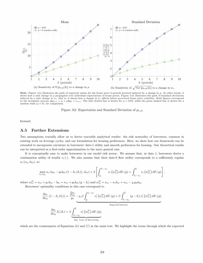
1 2 3 4 5 6 7 8 9 10

5

10

15

20

(a) Sensitivity of E [pt+k|It] to a change in µ

1 2 3 4 5 6 7 8 9 101

2

3

4

5

6

7

(b) Sensitivity of√

Var [pt+k|It] to a change in σε.

Note: Figure A2a illustrates the path of expected values for the house price k-periods forward induced by a change in µ. In other words, itshows how a unit change in µ propagates over individual expectations of house prices. Figure A2b illustrates the path of standard deviationsinduced by a unit change in σε, that is, it shows how a change in σε affects future perceived house price volatility. Both figures correspondto the stochastic process ∆pt+1 = µ + ρ∆pt + εt+1. The blue dotted line is drawn for ρ = 0.65, while the green dashed line is drawn for arandom walk (ρ = 0), for comparison.

Figure A2: Expectation and Standard Deviation of pt+k

forward.

A.5 Further ExtensionsTwo assumptions crucially allow us to derive tractable analytical results: the risk neutrality of borrowers, common inexisting work on leverage cycles, and our formulation for housing preferences. Here, we show how our framework can beextended to incorporate curvature in borrowers’ date-1 utility and smooth preferences for housing. Our theoretical resultscan be interpreted as a first-order approximation to the more general case.

It is conceptually easy to make borrowers in our model risk averse. We assume that, at date 1, borrowers derive acontinuation utility of wealth vi (·). We also assume that their date-0 flow utility corresponds to a sufficiently regularui (c0i, h0i), so

maxδi,h0i

ui (n0i − p0h0i (1− Λi (δi)) , h0i) + β

[∫ δi−χi

g

vi(wD

1i)dFi (g) +

∫ g

δi−χi

vi(wN

1i)dFi (g)

],

where wN1i = n1i + p1h0i − b0i = n1i + p0h0i (g − δi) and wD

1i = n1i − κih0i = n1i − χip0h0i.Borrowers’ optimality conditions in this case correspond to

∂ui∂c0i

(1− Λi (δi)) =∂ui∂h0i

p0−χiβ

∫ δi−χi

g

v′i(wD

1i)dFi (g) + β

∫ g

δi−χi

(g − δi) v′i(wN

1i)dFi (g)︸ ︷︷ ︸

Expected Return

,

∂ui∂c0i

Λ′i (δi) = β

∫ g

δi−χi

v′i(wN

1i)dFi (g)︸ ︷︷ ︸

Mg. Cost of Borrowing

,

which are the counterparts of Equations (6) and (7) in the main text. We highlight the terms through which the expected

A9

return and downpayment protection channels materialize. Equation (A1) corresponds in this case to

∂ui∂c0i

= β

∫ gδi−χi

v′i(wN

1i)dFi (g)

Λ′i (δi)=

∂ui∂h0i

p0 (1− Λi (δi))+ β

(−χi

∫ δi−χig

v′i(wD

1i)dFi (g) +

∫ gδi−χi

(g − δi) v′i(wN

1i)dFi (g)

)1− Λi (δi)

.

In this more general scenario, changes in borrowers’ beliefs only affect borrowers’ decisions insofar as they affect the expectedreturn and downpayment protection terms, which now include marginal utilities. We now sequentially study the impact ofseveral alternative modeling assumptions.

Final date risk aversion

We now assume that housing does not enter borrowers’ utility directly. In that case, we can combine borrowers’ optimalityconditions for housing and leverage to find a condition that generalizes (8). In particular, assuming κi = 0 for simplicity,

Λ′i (δi)1− Λi (δi)

= 1Ei[ (g−δi)v′i(wN

1i)|g≥δi]Ei[ v′i(wN

1i)|g≥δi]

,

whereEi[

(g − δi) v′i(wN

1i)∣∣ g ≥ δi]

Ei [v′i (wN1i )| g ≥ δi]

= Ei [g − δi| g ≥ δi] +Covi

[g − δi, v′i

(wN

1i)|g ≥ δi

]Ei [v′i (wN

1i )| g ≥ δi].

This more general expression includes a new term that separately affects borrowers’ leverage choices. Unfortunately, it isnot possible to analytically characterize how a change on borrowers’ beliefs affects the new term.

In the fixed house size scenario, a simple result can be found when borrowers are prevented from defaulting. In thatcase, the first-order condition for borrowing corresponds to

∂ui∂c0i

Λ′i (δi) = β

∫ g

g

v′i (n1i + p0h0i (g − δi)) dFi (g) .

In this case, it is easy to show that more optimistic borrowers, in a first-order stochastic dominance sense, decide to borrowmore. Intuitively, optimism is associated with a desire to transfer resources from the future and lower precautionary savings,both of which are associated with higher borrowing.

Smooth preferences for housing

In this case, we preserve borrowers’ risk neutrality and focus on the case in which preferences for housing are separable,

so ui (c0i, h0i) = vi (c0) + α2

(h0i − h̄

)2 and∂ui∂h0ip0

= αh0i−h̄p0

. Setting again κi = 0 for simplicity, we can express borrowers’optimality condition for housing as

h0i = h̄+ p0

α

(∂ui∂c0i

(1− Λi (δi))− β∫ g

δi

(g − δi) dFi (g)).

In the limit in which α → ∞, it must be that h0i → h̄, so changes in borrowers’ beliefs do not affect housing choices. Inthat case, borrowers’ make leverage choices according to

∂ui∂c0i

Λ′i (δi) = β

∫ g

δi

dFi (g) ,

as in the fixed house size scenario.

Alternative savings opportunities

Finally, although we have introduced consumption at date 0 as homebuyers’ alternative use of funds, they could be indifferentat the margin between their investment return on housing and alternative investment opportunities. If we assume thathouseholds have access to a savings opportunity with a constant gross returns Rs, their date 0 budget constraint becomes

n0i = p0h0i (1− Λi (δi)) + s, (A7)

A10

where s denotes savings. Therefore, at the optimum, the counterpart of Equation (A1) corresponds to

Rs =β∫ gδi−χi

dFi (g)Λ′i (δi)

=β[−χi

∫ δi−χig

dFi (g) +∫ gδi−χi

(g − δi) dFi (g)]

1− Λi (δi). (A8)

Homebuyers’ housing and borrowing decisions must at the margin yield a return Rs, so every argument in the paper remainsvalid. We adopt the formulation with consumption in the paper because for this alternative formulation to be well-behavedin the variable house size case, we would need to impose some curvature in the return Rs. By slightly changing the defaultformulation, one can allow for borrowers to save at date 0 to use some of those funds to avoid default at date 1. In thatcase, Equations (A7) and (A8) still determine the equilibrium after accounting for the different default behavior.

Role of Lenders’ Beliefs

Although our empirical findings build on cross-sectional variation on homebuyers’ beliefs, it may be valuable to separatelycharacterize the effect of changes in lenders’ beliefs on the equilibrium leverage choices of borrowers. We show that anincrease in lenders’ optimism can increase equilibrium leverage in both the fixed house size and the variable house sizescenarios. We assume that lenders have normally distributed beliefs with mean µL.

Proposition. (Parametric predictions of lenders’ beliefs.) In the variable house size scenario and the fixed house sizescenario, higher optimism by lenders, in the form of a higher average belief µL, holding all else constant, including borrowers’beliefs, can be associated with higher leverage.

We now formally show that a change in the average belief of lenders µL is associated with point-wise shifts in Λi (·) andΛ′i (·). Intuitively, when lenders become more optimistic, borrowers have access to cheaper funding. In the variable housesize scenario, we show that access to cheaper credit increases the maximum levered return that a borrower can achieve,generating a substitution effect towards higher leverage in equilibrium. In the fixed house size scenario, in addition to thesubstitution effect, there is an income effect that works in the opposite direction: lower interest rates make borrowers feelricher, which generates a force towards higher consumption and lower leverage. Therefore, our results show that shifts inthe beliefs of borrowers and lenders, when considered in isolation, can have opposite predictions for equilibrium leverage.

To provide comparative statics in the case of lenders’ beliefs, we must characterize the behavior of ∂Λi(δi)∂µL

and ∂Λ′i(δi)∂µL

.36

Formally, we find that both the LTV schedule offered by lenders and its derivative with respect to δi shift pointwise withchanges in µL:

∂Λi (δi)∂µL

=ηΦL

(δi−χi−µL

σL

)− (ηµL−δi)

σLφL(δi−χi−µL

σL

)+ ηφ′L

(δi−χi−µL

σL

)1 + r

> 0,

∂Λ′i (δi)∂µL

= (ηχi + (1− η) δi)(λ(δi − χi − µL

σL

)− δi − χi − µL

σL

) 1σL

φ(δi−χi−µL

σL

)1 + r

+[1− (ηχi + (1− η) δi)λ

(δi − χi − µL

σL

)] 1σL

φ(δi−χi−µL

σL

)1 + r

> 0,

where we use the fact that the pdf of the Normal distribution satisfies φ′ (x) = −xφ (x) and that 1 >

(ηχi + (1− η) δi)λ(δi−χi−µL

σL

)at any interior solution. Both results, when combined, imply that

d(

Λ′i(δi)1−Λi(δi)

)dµL

> 0.

In the variable house size scenario, Equation (A3) directly implies that upward point-wise shifts on Λ′i(δi)1−Λi(δi)

areassociated with a higher equilibrium leverage choice δi. Hence, a higher µL is associated with a higher equilibrium

36Note that we can express LTV schedules as

Λi (δi) =

ηΦL(δi−χi−µL

σL

)(µL − σL

φL

(δi−χi−µL

σL

)ΦL(δi−χi−µL

σL

))+(1− ΦL

(δi−χi−µL

σL

))δi

1 + r

=δi + (ηµL − δi) ΦL

(δi−χi−µL

σL

)− ησLφL

(δi−χi−µL

σL

)1 + r

A11

leverage choice δi. In the fixed house size scenario, Equation (A4) directly implies that upward point-wise shifts onu′i (n0i − p0h0i (1− Λi (δi))) Λ′i (δi) are associated with a higher equilibrium leverage choice δi. In this case,

∂ (u′i (·) Λ′i (δi))∂µL

= u′i (n0i − p0h0i (1− Λi (δi)))∂Λ′i (δi)∂µL

+ p0h0iu′′i (n0i − p0h0i (1− Λi (δi)))

∂Λi (δi)∂µL

Λ′i (δi) ,

whose sign is ambiguous. An increase in µL generates both a substitution and an income effect. More optimistic lendersoffer more attractive LTV schedules at the margin, so borrowers substitute towards higher leverage. More optimistic lendersoffer more attractive schedule, which makes borrowers effectively richer at date 0, reducing their need to borrow, whichreduces their equilibrium leverage.

A12

B Numerical SimulationAlthough we have derived our analytical results in the context of two polar scenarios, we now simulate an extensionof the model in which homebuyers have conventional CES preferences over consumption and housing (see, for example,Piazzesi, Schneider and Tuzel, 2007). In that case, the return sensitivity of housing investments is not determined by apotentially-binding housing size constraint, but instead arises endogenously from household preferences.

Our goal with this simulation is twofold. First, we show that we can recover the predictions of both polar scenarios forthe relationship between beliefs and leverage choices when employing more conventional preferences for housing. The factthat we can generate opposite predictions reinforces our motivation for the empirical analysis, which seeks to understandwhich effects dominate in the data. At the same time, we can provide a sense of the parameters that are consistent withthe predictions of the fixed house size scenario that we find in the data. Second, the extended model allows us to formallyreconcile the findings of this paper with the findings of Bailey et al. (2017), who document that more optimistic individualspurchase larger homes. Specifically, we show that in a world with partial collateral return sensitivity, it is possible to havemore optimistic individuals purchasing larger houses with lower LTV ratios.

Environment. We consider the same environment as in Section 3, except that we drop the housing constraint, givenby Equation (2), and instead introduce standard CES preferences between consumption and housing at date 0. Formally,homebuyers solve the following problem:

maxc0i,δi,h0i

J (c0i, δi, h0i)

where

J (c0i, δi, h0i) = U (c0i, h0i) + βp0h0i

∫ g

δi

(g − δi) dFi (g)− λ0i (c0i + p0h0i (1− Λ (δi))− n0i) ,

and whereU (c0i, h0i) = (ui (c0i, h0i))1−γ

1− γ and ui (c0i, h0i) =[αc

ε−1ε

0i + (1− α)hε−1ε

0i

] εε−1

where σ corresponds to the elasticity of substitution between consumption and housing.37 The lenders’ LTV schedule isgiven by

Λi (δi) =η∫ δiggdFL (g) + δi

∫ gδidFL (g)

1 + r,

with FL (·) normally distributed. Using the fact that c0i = n0i − p0h0i (1− Λ (δi)), the solution of the model can be foundby solving the following system of two equations and two unknowns, δi and h0i:

∂ui (c0i, h0i)∂h0i

= p0β (1− Fi (δi))

(1− Λ (δi)

Λ′ (δi)−

∫ gδi

(g − δi) dFi (g)∫ gδidFi (g)

)∂ui (c0i, h0i)

∂c0i= β

1− Fi (δi)Λ′ (δi)

Parameters. Although our model is highly stylized, we stay close to existing quantitative models with housing whenselecting parameters for our simulation. We interpret the single period in the model as five years. Our choices for preferenceparameters build on Piazzesi, Schneider and Tuzel (2007). We select a static elasticity of substitution between consumptionand housing of ε = 1.25, an EIS/Risk Aversion parameter of γ = 1 (corresponding to log-utility), and α = 0.5, which wouldimply equal shares of consumption and housing services in a static setup. We use a recovery rate for lenders of η = 0.75after default, consistent with Campbell, Giglio and Pathak (2011). We normalize p0 = n0i = 1, so that lenders’ date-0resources are equal to unity. We assume that lenders’ average belief is µL = 1.1 and that both homebuyers and lenders havethe same standard deviation of beliefs, σB = σL = 0.25. We assume that r = 1.15 ≈ 1.035 and consider two scenarios: onewith patient homebuyers/borrowers (β = 0.95 ≈ 0.995), and one with impatient homebuyers/borrowers (β = 0.7 ≈ 0.945).We set (effectively non-binding) upper and lower thresholds for all distributions g = 0.1 and g = 2.

Results. We illustrate the results of our simulation in Figure A3. The left panels show the relationship between impatientborrowers’ beliefs and choices for LTV ratio and house size. Over almost the entire range of beliefs considered, µB ∈ [1, 1.2],we find a negative relationship between borrowers’ beliefs and leverage choices, consistent with the empirical results inSection 3. Only when borrowers are very optimistic, we find that LTV ratios are increasing in borrowers’ beliefs. In

37This preference specification implies that Uc = αu1ε−γ

i c− 1ε

0i and Uh = (1− α)u1ε−γ

i h− 1ε

0i .

A13

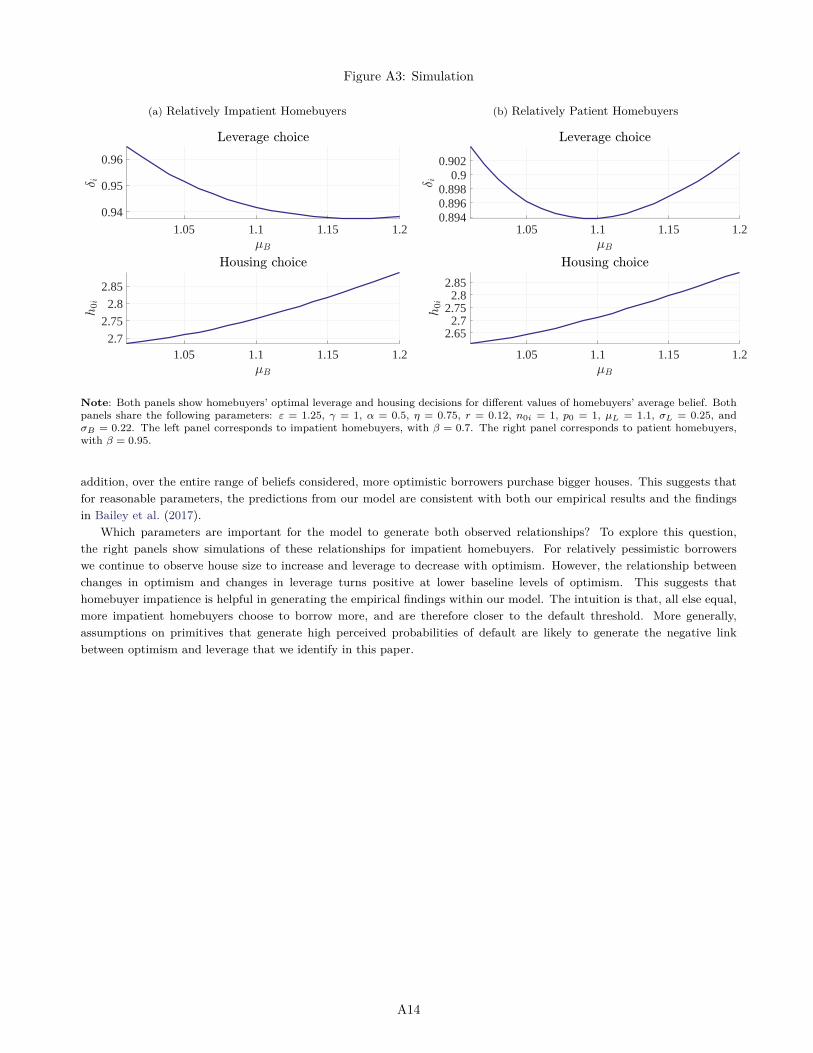
Figure A3: Simulation

(a) Relatively Impatient Homebuyers

1.05 1.1 1.15 1.2

0.94

0.95

0.96

1.05 1.1 1.15 1.22.7

2.75

2.8

2.85

(b) Relatively Patient Homebuyers

1.05 1.1 1.15 1.20.8940.8960.898

0.90.902

1.05 1.1 1.15 1.2

2.652.7

2.752.8

2.85

Note: Both panels show homebuyers’ optimal leverage and housing decisions for different values of homebuyers’ average belief. Bothpanels share the following parameters: ε = 1.25, γ = 1, α = 0.5, η = 0.75, r = 0.12, n0i = 1, p0 = 1, µL = 1.1, σL = 0.25, andσB = 0.22. The left panel corresponds to impatient homebuyers, with β = 0.7. The right panel corresponds to patient homebuyers,with β = 0.95.

addition, over the entire range of beliefs considered, more optimistic borrowers purchase bigger houses. This suggests thatfor reasonable parameters, the predictions from our model are consistent with both our empirical results and the findingsin Bailey et al. (2017).

Which parameters are important for the model to generate both observed relationships? To explore this question,the right panels show simulations of these relationships for impatient homebuyers. For relatively pessimistic borrowerswe continue to observe house size to increase and leverage to decrease with optimism. However, the relationship betweenchanges in optimism and changes in leverage turns positive at lower baseline levels of optimism. This suggests thathomebuyer impatience is helpful in generating the empirical findings within our model. The intuition is that, all else equal,more impatient homebuyers choose to borrow more, and are therefore closer to the default threshold. More generally,assumptions on primitives that generate high perceived probabilities of default are likely to generate the negative linkbetween optimism and leverage that we identify in this paper.

A14

C Non-Parametric Predictions

C.1 Theoretical resultsWhile the parametric assumption underlying Propositions 1 and 2 are natural, given that the distribution of g is unimodaland symmetric in the data, these results impose a priori unnecessary distributional restrictions. An alternative approach isto consider cross-sectional comparisons among borrowers that do not rely on parametric assumptions. This approach usesthe ability to potentially observe shifts of the whole distribution of beliefs, which is a unique feature of our empirical setup.

In general, there are numerous ways in which one borrower may be “more optimistic” than another in a non-parametricsense. For example, two borrowers could disagree primarily about the probability of very large declines or very largeincreases in house prices. In this section, we identify the appropriate definition of stochastic dominance that allows us toprovide unambiguous directional predictions for borrowers’ leverage choices across both the fixed house size and variablehouse size scenarios. Because of the inherent difficulties with establishing general comparisons between infinite-dimensionaldistributions, our non-parametric results only provide a partial order when comparing borrowers in the data — there aremany pairwise comparisons of borrowers’ distributions that cannot be ranked according to the appropriate dominancenotion.

We use three different stochastic orders to define optimism. Given two distributions with cumulative distributionfunctions Fj (·) and Fi (·) with support

[g, g], we define truncated expectation stochastic dominance, first-order stochastic

dominance and hazard rate dominance as follows:

1. Truncated expectation stochastic dominance: Fj stochastically dominates Fi (borrower j is more optimisticthan i) in a truncated expectation sense if

Ej [g| g ≥ δ] ≥ Ei [g| g ≥ δ] , ∀δ ∈[g, g].

2. First-order stochastic dominance: Fj stochastically dominates Fi (borrower j is more optimistic than i) in afirst-order sense if

Fj (δ) ≤ Fi (δ) , ∀δ ∈[g, g].

3. Hazard rate stochastic dominance: Fj stochastically dominates Fi (borrower j is more optimistic than i) in ahazard rate sense if

fj (δ)1− Fj (δ) ≤

fi (δ)1− Fi (δ) , ∀δ ∈

[g, g].

All three definitions capture different notions of optimism. We show in Appendix A.3 that if Fj (·) dominates Fi (·) in ahazard rate sense, then Fj (·) also dominates Fi (·) in a first-order and a truncated expectation sense. The converse is nottrue: first-order stochastic dominance and truncated expectation dominance do not imply hazard rate dominance. FigureA4 illustrates the relation between the different orders. Hazard rate dominance is equivalent to saying that 1−Fj(g)

1−Fi(g)is

increasing on g. It captures the idea that optimists are increasingly optimistic about higher house price growth realizations.

Figure A4: Relation Between Stochastic Orders

Variable House Size Fixed House Size

Ej[g| g ≥ δ̃

]≥ Ei

[g| g ≥ δ̃

],∀δ̃ ⇒ LTVj ≥ LTVi

Truncated Expectation Stochastic Dominance

Fj

(δ̃)≤ Fi

(δ̃),∀δ̃ ⇒ LTVj ≤ LTVi

First Order Stochastic Dominance

fj(δ̃)1−Fj(δ̃)

≤ fi(δ̃)1−Fi(δ̃)

,∀δ̃

Hazard Rate Stochastic Dominance

We have shown that in the variable house size scenario, when κi = 0, there are clear predictions for the leverage choicesacross two borrowers whose belief distributions could be ranked according to truncated-expectation stochastic dominance.We also showed that in the fixed house size scenario, clear predictions were obtained for belief distributions that could beranked according to first-order stochastic dominance. However, neither of these dominance concepts implies the other, so itis unclear how to compare belief distributions if we are ex-ante agnostic about whether the fixed house size or the variable

A15

house size scenario applies. Therefore, we adopt hazard rate dominance as the appropriate definition of optimism thatallows to test non-parametrically for the effect of beliefs on leverage regardless of the underlying scenario, as formalized inProposition 3.

Proposition 3. (Non-parametric predictions.) Compare two borrowers i and j with different distributions Fi (·) and Fj (·)about the growth rate of house prices changes.a) In the variable house size scenario, if Fj (·) dominates Fi (·) in a hazard rate sense (or in a truncated expectation sensewhen κi = 0), all else equal, borrower j chooses a higher LTV ratio and a larger house than borrower i.b) In the fixed house size scenario, if Fj (·) dominates Fi (·) in a hazard rate sense (or in a first-order sense), all else equal,borrower j chooses a lower LTV ratio and lower consumption than borrower i.

Proposition 3 shows that borrowers’ optimism, measured as hazard rate dominance, has opposite predictions in the polarscenarios we consider for any value of κi. More optimistic borrowers take on more leverage in the variable house sizescenario, but they take on less leverage in the fixed house size scenario. These results generalize the insights from thecase with normally distributed beliefs, but they are not exactly identical. We show here that, when beliefs are normallydistributed, a distribution with a higher mean dominates in a hazard rate sense a distribution with a lower mean (holding itsvariance constant). Hence, when comparing means in the normal case, the results of Proposition 1 are implied by those ofProposition 3. However, we also show that, in the normal context, a distribution with a higher variance does not dominatein a hazard rate sense a distribution with a lower variance (holding its mean constant). This illustrates that hazard ratedominance is only a sufficient (not a necessary) condition to derive unambiguous predictions for the relationships betweenbeliefs and leverage choice.

Proof of Proposition 3. (Non-parametric predictions)

In the variable house size scenario, it follows that an upward pointwise shift in 1 − Fi(δ̃), ∀δ̃, is associated with a lower

equilibrium value of δi. If the beliefs of borrower j first-order stochastically dominate the beliefs of borrower i (borrower jis more optimistic), then Fj

(δ̃)< Fi

(δ̃)and 1−Fj

(δ̃)> 1−Fi

(δ̃), which implies that borrower j takes on more leverage

on equilibrium.In the variable house size scenario, from Equation (8), it follows that an upward pointwise shift in −χi

Fi(δ̃−χi)1−Fi(δ̃−χi) +

Ei[g| g ≥ δ̃ − χi

], ∀δ̃ is associated with a higher equilibrium value of δi. To compare the leverage choices of two different

borrowers i and j, it is thus sufficient to show that Fj �HRD Fi implies that

Ej[g| g ≥ δ̃

]− Ei

[g| g ≥ δ̃

]> 0, ∀δ̃,

to conclude that the more optimistic borrower j takes on more leverage, since hazard-rate dominance implies first orderstochastic dominance, which trivially implies that Fj(δ̃−χi)

1−Fj(δ̃−χi) <Fi(δ̃−χi)

1−Fi(δ̃−χi) . To this purpose, we can define h (δ) as

h(δ̃)

= Ej[g| g ≥ δ̃

]− Ei

[g| g ≥ δ̃

].

We can express the derivative of h(δ̃)as

h′(δ̃)

=∂Ej

[g| g ≥ δ̃

]∂δ

−∂Ei

[g| g ≥ δ̃

]∂δ

=fj(δ̃)

1− Fj(δ̃) [Ej [g| g ≥ δ̃]− δ̃]− fi

(δ̃)

1− Fi(δ̃) [Ei [g| g ≥ δ̃]− δ̃]

=

(fj(δ̃)

1− Fj(δ̃) − f

(δ̃)

1− F(δ̃))︸ ︷︷ ︸

>0

Ej[g| g ≥ δ̃

]+

fi(δ̃)

1− Fi(δ̃)h (δ̃) . (A9)

When δ̃ → 0, it follows from hazard-rate dominance that Ej [g] − Ei [g] > 0. Note that all elements in (A9) are strictlypositive under hazard rate dominance, which implies that the solution to the ordinary differential equation for h

(δ̃)must

be weakly positive everywhere, implying that h(δ̃)is positive, which shows our claim.

A16

C.2 Non-Parametric TestThe empirical results presented in Sections 3.3 and 3.4 test the predictions from our model under the assumptionthat individuals’ beliefs about future house price changes are normally distributed. We argued that this is a realisticapproximation, given the shape of the distribution of actual house price changes. In Section C.1, we also derived non-parametric predictions on the relative mortgage leverage choices of individuals with arbitrary belief distributions. Inparticular, we showed that an individual whose belief distribution dominated that of an otherwise identical individual inthe sense of hazard rate dominance would choose higher leverage in the variable house size scenario, but lower leverage inthe fixed house size scenario.

While we are not able to measure the full belief distribution of each individual, we can compare how the leveragechoices of individuals vary with the full distribution of the house price experiences of their friends.38 Specifically, weconduct pairwise comparisons of the distributions of the house price experiences of all friends (and all out-of-commutingzone friends) of individuals purchasing houses in the same county in the same month, and who borrow from the samelender. We then test whether one distribution dominates the other in a hazard rate dominance sense. We only focus oncounty-month-lender combinations with at least three mortgage originations: at the average (median) such combination, wehave 9.8 (5) mortgage originations. Of all the pairwise comparisons across these originations, we can rank the distributionof all friends’ house price experiences in a hazard rate sense for 3.5% of transaction pairs, and the distributions of out-of-commuting zone friends’ house price experiences for 8.1% of transaction pairs. When comparing the mortgage leveragechoices across the individuals with a clear ranking using the experience distribution of all friends, we find that individualswith an experience distribution that is hazard rate dominant will choose 90 basis points lower leverage; this difference ishighly statistically significant. When comparing the experience distribution of individuals’ out-of-commuting zone friends,those with a hazard rate dominant distribution choose a 68 basis points lower leverage. Both of these results provideadditional evidence that the fixed house size scenario, in which collateral choices are return insensitive, is dominant in thedata.

38This test builds on the survey evidence in Section 3.2, which showed that, on average, the first and second moments of the houseprice experiences of an individual’s friends affect the corresponding moments of her belief distribution about future house price changes.The assumption underlying the test in this section is that additional moments of the distribution of individuals’ friends’ house priceexperiences will also shift the corresponding moments of those individuals’ belief distribution.

A17

D Additional Evidence

D.1 Distribution of County-Level House Price ChangesFigure A5 shows the distribution of county-year level annual house price changes in the United States between 1993 and2017, as measured by Zillow. The distribution is unimodal and approximately symmetric, motivating our choice of modelingbeliefs about house price changes to follow a normal distribution.

Figure A5: Distribution of House Price Changes (1993-2017)

0.0

2.0

4.0

6.0

8D

ensi

ty

-30 -20 -10 0 10 20 3012-Month County-Level House Price Change (%)

Note: Figure shows the distribution of annual county-level house price changes in the United States since 1993, as measured by Zillow.

D.2 Transactions Over TimeFigure A6 shows the number of transactions per calendar year in the baseline sample studied in Section 2.1.

Figure A6: Number of Transactions

010

020

030

0N

umbe

r of T

rans

actio

ns (T

hous

ands

)

2008

2009

2010

2011

2012

2013

2014

Note: Figure shows the number of transactions by purchase year in our matched transaction-Facebook sample.

A18

D.3 Hedonic Valuation ModelIn Section 3.4, we address the concern that the relationship between optimism and leverage is the result of more optimisticindividuals not being able to increase their mortgage amount. The concern is that these optimistic individuals overpayfor their properties, yet banks determine maximal mortgage amounts based on their own assessed value of the property.To rule out such concerns, we control for the extent of overpayment by individual homebuyers in column 4 of Table 5. Incolumn 5 of that Table, we restrict the sample to transactions where the homebuyer paid less for the property than itspredicted value. In this Appendix, we discuss our procedure of arriving at the automated valuation of the property, anddescribe how we construct our measure of overpayment. Specifically, we begin by running a hedonic regression of the log ofthe transaction price on observable characteristics of the property (see Giglio, Maggiori and Stroebel, 2015; Stroebel, 2015,for similar hedonic pricing approaches):

log (Pricei,t) = α+ βXi,t + ψzipi,t + εi,t.

We control flexibly for the property characteristics that are observable in our data set: property size, lot size, propertyage, property type, and whether the property has a pool. For property size and lot size, we include year-specific dummyvariables for 50 quantiles of the distribution. For the other variables, we include year-specific dummy variables for each ofthe possible values. In addition, we include zip code by month fixed effects, to control for localized time-trends in houseprices. This regression has an R-Squared of 83.6%, which is high, particularly given the fact that we observe prices inbuckets. We then calculate, for each property, the predicted price based on this hedonic pricing model. We then constructa measure of whether a particular buyer “overpaid” relative to the predicted value as:

Overpay = 100× TransactionPrice− PredictedPricePredictedPrice

.

D.4 County Wealth vs. County House Price ChangesOne concern addressed in Section 3.4 was that wealthier people would have friends in wealthier counties. If these wealthiercounties also experienced house price appreciation, then the estimates of β1 in Equation R1 might be picking up thatwealthier people make larger downpayments. We argued that this is unlikely to be the explanation of our results, sinceno persons’ friend experience consistently higher or lower house price experiences. Specifically, we argued that it was notthe case that wealthier regions always have higher house price growth — in some years, wealthier counties see larger houseprice increases, in other years they see smaller house price increases. In this Appendix, we provide the evidence for theseclaims.

Specifically, to measure household wealth at the county level, we use county-level measures of average household netwealth constructed by Applied Geographic Solutions for the years 2011 to 2016.39 The ranking of counties in their netwealth is stable over time: counties that were relatively wealthy in 2011 were generally relatively wealthy in 2014 — seePanel (a) of Figure A7. However, house price changes over the prior 24 months were quite different between 2011 and 2014:counties that had a relatively positive house price experience in the 24 months leading up to January 2011 had a relativelynegative house price experience in the 24 months leading up to January 2014 – see Panel (b) of Figure A7. As a result, therelationship between county-level wealth and house price growth depends on time horizon considered. For example, Panel(c) shows that in January 2011, wealthier counties had experienced relatively larger house price declines over the previous24 months while Panel (d) shows that in January 2014, wealthier counties had seen larger relative house price increases.

The instability of the relationship between county wealth and house price experiences is a persistent pattern in ourdata. To document this, we calculate, for every month between January 2008 and December 2016, the correlation betweennet wealth and house price changes over the previous 24 months. Panel (e) of Figure A7 plots that correlation over time.One can see that the correlation between wealth and past house price experiences is zero or negative until January 2013,after which it becomes positive. Due to the strong persistence in county net wealth over time, this pattern is unaffected bywhen we measure of county level net wealth.

39Applied Geographic Solutions defines net worth as the difference between assets and debts of households at the county level,where assets include transactions accounts, life insurance with cash value, primary residence value, and debts include mortgage andcredit card debt. This measure is constructed using a number of data sets, including from the American Community Survey, the U.S.Census, IRS statistics, and credit bureau data.

A19

Figure A7: County Level Wealth and House Price Changes

(a) Correlation in County-Level Net Wealth20

0000

4000

0060

0000

8000

0010

0000

012

0000

0N

et W

ealth

in 2

014

200000 400000 600000 800000 1000000 1200000Net Wealth in 2011

(b) County Wealth vs. House Price Changes

-.10

.1.2

.324

m D

elta

HP

in 2

014-

01

-.4 -.2 0 .2 .424m Delta HP in 2011-01

(c) County Wealth vs. House Price Changes: January 2011

-.15

-.1-.0

50

24-M

onth

Hou

se P

rice

Cha

nge,

Up

to J

anua

ry 2

011

200000 400000 600000 800000 1000000 1200000Net Wealth in 2011

(d) County Wealth vs. House Price Changes: January 2014

-.05

0.0

5.1

.15

.224

-Mon

th H

ouse

Pric

e C

hang

e, U

p to

Jan

uary

201

4

200000 400000 600000 800000 1000000 1200000Net Wealth in 2011

(e) Correlation between House Price Changes and Net Wealth

-.4-.2

0.2

.4

01jul2008 01jul2010 01jul2012 01jul2014 01jul2016Month

Corr Delta HP vs. 2011 NW Corr Delta HP vs. 2014 NW

Note: Panel (a) shows a binned scatter plot of counties’ average net wealth in 2011 and 2014. Panel (b) shows a binned scatter plotof counties’ house price changes in the 24 months up to January 2011 and the 24 months up to January 2014. Panels (c) and (d) showbinned scatter plots of county-level wealth in 2011 and county-level house price changes in the 24 months prior to January 2011 andprior to January 2014, respectively. Panel (e) shows a monthly time-series in the correlation between county-level net wealth (eithermeasured in 2011 or in 2014) and the counties’ house price changes over the previous 24 months.

A20

D.5 Downpayments and Expected DefaultAs discussed in Section 4, many personal financial advice websites and blogs discuss the tradeoffs between making largerand smaller downpayments. Many of these highlight explicitly the tradeoffs that we formally model in Section 1. Forexample, the real estate brokerage website Home Point Real Estate describes one of the benefits of high leverage as follows:

This last reason for putting down a small down payment is kind of twisted, but sadly practical. I doubt weare going to have any down turn in the market soon, and I really doubt it will be like the one we just camethrough if it does come; but the less you put down the less you lose. Yet, if you are upside down on your homeand have to walk away (or lose to foreclosure) the less down payment you put into it the less you lose.

Reuters (2011) outlines similar reasons for making a smaller downpayment:

Even if you have the money for a bigger down payment, there can be good reasons to save your cash. Mortgagerates continue to skirt all-time lows: Why not put your money to work for yourself and borrow as much as youcan reasonably afford, on a monthly basis, at today’s rates? You can put the money you’re not paying into adown payment to work elsewhere. If home values rise, you will have done your best to leverage a small downpayment into bigger equity. If they fall, you’ll have less skin in the game, and that could put more pressure onyour banker to improve your loan terms lest you walk away.

US News (2017) described the benefits of a smaller downpayment as follows:

The last major housing crash scared some people away from low down payments after many homeownersfound themselves owing more than their homes were worth when values plummeted. But even a 20 percentdown payment won’t protect you against a 50 percent drop in home values. In fact, if you lost your home toforeclosure or did a short sale, you may have lost less money if you made a small down payment.

MK Real Estate (2016) describes why making smaller downpayments is the more conservative choice for home buyersworried about potential house price drops.

The link between the economy and home prices is the third reason to consider a small down payment. Ingeneral, as the U.S. economy improves, home values rise. When the U.S. economy sags, home values sink.Buyers with large down payments find themselves over-exposed to economic downturns compared to buyerswhose down payments are small.Consider the purchase of a $400,000 home and two home buyers, each with different ideas about how to buy ahome. One buyer makes a 20% down payment to avoid Private Mortgage Insurance (PMI). The other buyerwants to stay as liquid as possible, and puts down just 3.5%. The first buyer takes $80,000 from the bank andconverts it to illiquid home equity. The second buyer puts $14,000 into the home.Over the next few years, the economy falters. Our two buyers lose 20% of the value of each of their homes,bringing their values down to $320,000. Neither buyer has any equity left. Our first buyer lost all $80,000 oftheir money. That money is lost and cannot be recouped except through the housing market’s recovery. Thesecond buyer lost only $14,000. While the second buyer’s home is “underwater,” with more money owed onthe home than the home is worth, the bank has the risk of loss and not the borrower.Let’s say that both borrowers default and no longer make their payments. Which homeowner will the bankbe more likely to foreclose upon? It’s counter-intuitive, but the buyer who made a large down payment is lesslikely to get relief during a time of crisis and is more likely to face foreclosure. A bank’s losses are limited towhen the home is sold at foreclosure. The homeowner’s twenty percent home equity is already gone, so theremaining losses (legal and home prep costs) are easily absorbed by the bank. Foreclosing on an underwaterhome will lead to great losses. All of the borrower’s money is already lost. The bank will not only have legaland home prep costs, but will also have to write down $66,000 in lost value.Conservative borrowers recognize that risk increases with the size of the down payment. The smaller your downpayment, the smaller your risk.

D.6 Downpayment Motivation SurveyIn Section 4.2, we described results from our Downpayment Motivation Survey. In this Appendix, we provide additionalinformation on the respondent demographics, and more details on how the responses vary with these demographics. Forcomplete disclosure, the full data set is available from the authors upon request.

A21

We ran two waves of the survey between September 19, 2017, and September 21, 2017. The survey was designed usingthe SurveyMonkey survey platform. Each wave was targeted at approximately 800 homeowners, and no additional filtersfor the target audience were selected. In each wave, respondents were presented with two different house price growthscenarios, and asked to select one of three different mortgage choices for each house price scenario. In Table A1, weshow the changes in the downpayment recommendation between the optimistic and the pessimistic scenario (“DecreasedDownpayment” represents individuals who suggested a smaller downpayment in the more pessimistic house price scenario).

Table A1: Downpayment Motivation Survey - Results by Demographics

TotalDecreased

DP

Same 

DP

Increased

DPTotal

Decreased

DP

Same 

DP

Increased

DP

All 826 20.5% 69.4% 10.2% 794 14.0% 77.6% 8.4%

Income   $0 to $9,999 17 11.8% 82.3% 5.9% 12 8.3% 91.7% 0.0%   $10,000 to $24,999 38 13.2% 63.2% 23.7% 37 10.8% 62.2% 27.0%   $25,000 to $49,999 92 14.1% 76.1% 9.8% 84 8.3% 88.1% 3.6%   $50,000 to $74,999 56 23.2% 73.2% 3.6% 46 15.2% 60.9% 23.9%   $75,000 to $99,999 35 20.0% 71.4% 8.6% 40 17.5% 80.0% 2.5%   $100,000 to $124,999 15 6.7% 86.7% 6.7% 18 16.7% 83.3% 0.0%   $125,000 to $149,999 50 26.0% 66.0% 8.0% 51 7.8% 84.3% 7.8%   $150,000 to $174,999 103 28.2% 59.2% 12.6% 88 13.6% 77.3% 9.1%   $175,000 to $199,999 122 22.1% 68.0% 9.8% 122 13.1% 80.3% 6.6%   $200,000 and up 117 18.0% 75.2% 6.8% 108 16.7% 74.1% 9.3%   Prefer not to answer 125 16.0% 76.8% 7.2% 137 16.8% 77.4% 5.8%

Age   18‐29 51 23.5% 62.8% 13.7% 42 14.3% 78.6% 7.1%

   30‐44 168 18.5% 68.4% 13.1% 154 11.7% 76.6% 11.7%

   45‐59 215 16.7% 76.3% 7.0% 216 16.2% 76.4% 7.4%

   60+ 336 21.4% 70.5% 8.0% 331 13.0% 79.2% 7.8%

Gender   Male 324 19.4% 67.9% 12.6% 294 14.3% 77.2% 8.5%

   Female 446 21.5% 70.8% 7.7% 449 9.2% 83.1% 7.7%

Region   East North Central 130 21.5% 70.8% 7.7% 130 9.2% 83.1% 7.7%   East South Central 46 15.2% 73.9% 10.9% 41 9.8% 82.9% 7.3%   Middle Atlantic 94 18.1% 73.4% 8.5% 90 16.7% 75.6% 7.8%   Mountain 58 13.8% 82.8% 3.5% 63 14.3% 74.6% 11.1%   New England 44 13.6% 77.3% 9.1% 47 12.8% 78.7% 8.5%   Pacific 133 23.3% 65.4% 11.3% 111 10.8% 79.3% 9.9%   South Atlantic 131 22.1% 64.1% 13.7% 134 18.7% 72.4% 9.0%   West North Central 59 17.0% 78.0% 5.1% 55 18.2% 76.4% 5.4%   West South Central 74 20.3% 71.6% 8.1% 68 11.8% 79.4% 8.8%

Wave 1 Wave 2

Note: Table shows responses in the Downpayment Motivation Survey separately by the reported demographic of the respondents.The results show how the downpayment recommendation changes in the pessimistic house price scenario relative to the optimistichouse price scenario.

A22