1  

Household Balance Sheets, Consumption, and the Economic Slump

Atif Mian Princeton University and NBER

Kamalesh Rao

MasterCard Advisors

Amir Sufi University of Chicago Booth School of Business and NBER

February 2013

Abstract

During the Great Recession in the United States, wealth shocks coming from high ex ante leverage and the sharp decline in house prices were very unequal across the country. We first document these large geographic differences in wealth shocks, and then investigate the consumption consequences. We find an elasticity of consumption with respect to housing net worth shocks of 0.6 to 0.8, and an average marginal propensity to consume of 5 to 7 cents per dollar loss in housing net worth. There are large differences in MPCs across the population: poorer and more highly levered households cut spending by substantially more per lost dollar of housing net worth. Our findings highlight the importance of debt, the distribution of wealth, and geography in explaining the sharp and unequal decline in consumption from 2006 to 2009. * Lucy Hu, Ernest Liu, Christian Martinez, Yoshio Nozawa, and Calvin Zhang provided superb research assistance. We are grateful to the National Science Foundation, the Initiative on Global Markets at Chicago Booth, and the Fama-Miller Center at Chicago Booth for funding. Seminar participants at Chicago Booth, Columbia Business School, Harvard, MIT Sloan, MIT Economics, NYU Stern, Stanford GSB, UC Berkeley, UCLA, UC San Diego, and the NBER Monetary Economics meeting provided valuable feedback. The results or views expressed in this study are those of the authors and do not reflect those of the providers of the data used in this analysis. Corresponding authors: Mian: (609) 258-6718, atif@princeton.edu; Sufi: (773) 702 6148, amir.sufi@chicagobooth.edu   

2  

How does consumption respond to large negative shocks to household wealth? Do

households with different levels of wealth have different marginal propensities to consume out of

a dollar lost? These questions are fundamental in macroeconomics and finance, and the answers

have profound implications for how we model the economy, how wealth shocks translate into

business cycle fluctuations, and how policy should respond when asset prices collapse.

For example, many traditional models of the macro-economy adopt a representative agent

framework, implicitly assuming that individual households are hedged against idiosyncratic or

household-specific wealth shocks. However, if this assumption is grossly violated in data, then

we may need to adopt heterogeneity in our models. Further, if households across the wealth

distribution do not have the same marginal propensity to consume out of changes in wealth, then

the distribution of dollar losses across the economy may affect aggregate consumption.

These questions are especially important when considering severe recessions. In the

United States, both the Great Depression and Great Recession were precipitated by a collapse in

asset prices and a large drop in consumption.1 Many scholars have modeled the sharp decline in

consumption by assuming a discount rate shock in a representative agent framework. However,

recent theoretical research inspired by the Great Recession has explicitly used heterogeneity in

wealth, debt, or liquidity across households to explain the large decline in spending (Eggertsson

and Krugman (2012), Guerrieri and Lorenzoni (2012), and Midrigan and Philippon (2012)).

In this study, we provide evidence that heterogeneity in wealth shocks is crucial for

explaining the spending patterns of households during the Great Recession. We use a novel data

set of consumption and wealth shocks at the county level, and we exploit geographic variation

across U.S. counties in the shock to household net worth coming from high ex ante leverage and

                                                            1 See for example Temin (1976) and Olney (1999) for evidence on the Great Depression. For the Great Recession, NIPA and Census retail sales data show a definitive collapse in durable consumption even before the fall of 2008.

3  

the collapse in house prices. We find evidence that household spending is very responsive to

housing net worth shocks. We estimate an elasticity of consumption with respect to the drop in

housing net worth between 0.6 and 0.8. Alternatively, we use the cross-section of counties to

measure a contemporaneous marginal propensity to consume out of housing wealth of between 5

and 7 cents on the dollar.

Further, we show that the response of households to the same dollar hit to housing net

worth depends on their balance sheet position at the start of the recession. For the same dollar

decline in home equity, poorer households and more highly levered households cut spending by

significantly more. In other words, the marginal propensity to consume out of housing wealth is

substantially higher for poorer and more highly levered households. For example, households

with annual income less than $35 thousand have an MPC that is three times as large as the MPC

for households with more than $200 thousand in income. Households in the 90th percentile of

the leverage distribution have an MPC that is twice as high as households in the 10th percentile

of the leverage distribution.

The heterogeneity of MPCs across households implies that the distribution of losses when

asset prices collapse is important for understanding the magnitude of the consumption drop. For

example, the presence of debt may concentrate the losses on households with the highest MPC,

making the drop in household spending especially severe. We provide evidence on this effect by

showing that the MPC was largest among households that went underwater on their mortgages.

Our results imply that heterogeneity across households in the exposure to housing net

worth shocks is important for explaining the dynamics of consumption during the Great

Recession. Further, households displayed substantial variation in their consumption response to

4  

the same home value decline. The latter result suggests that the distribution of wealth and debt in

an economy is important in explaining how aggregate spending responds to wealth shocks.

The rest of this paper proceeds as follows. In the next section, we develop theoretical

predictions based on extant research relating consumption to wealth shocks. Section 2 presents

the data and summary statistics. Section 3 discusses variation in net worth shocks across

counties. Sections 4 and 5 present the results, and Section 6 concludes.

1. Theory

How does a severe shock to net worth – like the collapse of house prices in the United

States during the Great Recession – impact consumption and the real economy? Consider an

economy where households i’s net wealth at time t is given by:

(1)

The first three terms on the right hand side represent the market values of stocks, bonds,

and housing, respectively, while the last term represents the value of debt borrowed by the

household.

Imagine a severe negative shock to wealth unexpectedly strikes the economy. The wealth

shock changes asset prices in the economy, which results in a change in household i's net worth.

Given the household's initial asset holdings, we can compute the change in household net worth

(in dollars) by:

∆ ∗ ∆ ∗ ∆ ∗ (2)

where ∆ , ∆ and ∆ represent price growth in stocks, bonds, and housing,

respectively. Throughout, we use the symbol ∆ for growth, or percent change, in a variable. The

debt term disappears from equation (2) because we are assuming that the the value of debt is

5  

fixed in nominal terms, which implicitly disallows default, additional levering, or paying down

debt. In equation (2), we focus on the change in net worth in dollar units, but we can define the

change in net wealth in percentage terms as ∆ . We would then simply divide

both sides of equation (2) through by the lagged value of net worth for this household. The

growth in net worth will be a key element of our empirical approach below.

How should household consumption respond to the wealth shock? There is a large

literature on this question, and we outline the basic hypotheses below.

A. The complete risk-sharing hypothesis

Suppose households in the economy have CRRA preferences. Then, under the

assumption of complete risk-sharing across households, growth in consumption is completely

unrelated to idiosyncratic wealth shocks (e.g., Cochrane (1991)). In particular, any cross-

sectional regression relaying consumption growth to net worth growth of the form:

∆ ∗ ∆ (3)

should give us 0.

Equation (3) is derived under the assumption of complete markets. However papers such

as Lucas (1991), Telmer (1993), Aiyagari and Gertler (1991), and Heaton and Lucas (1992,

1994a, 1994b) show that one can get close to full insurance under weaker assumptions. In

particular, the environment can have incomplete markets and limited borrowing capacity. But as

long as people can trade in a few basic securities, we get close to full insurance. The possibility

of informal insurance mechanisms and government transfer programs provides another rationale

for consumption insurance. 

6  

There is an additional reason that households are naturally hedged against movements in

house prices, and hence for to be close to zero. Housing differs from other assets because it

also a consumption good. As a result, for a homeowner who expects to live in his home for a

long time or who cares about his offspring to live in a similar home, an increase in house prices

does not make him richer because it also increases the implicit rental cost of housing. A similar

argument works when house prices decline. Under this view, households should not be

responsive to movements in net worth driven by home values.2

A corollary of the above argument is that a reduction in house prices may increase non-

housing consumption for households that were planning on increasing their housing consumption

in the future. An example would be renters planning on buying a bigger condominium or home

in the future. They actually feel richer when house prices decline. Homeowners that were

planning on downsizing may decrease their non-housing consumption as they now feel poorer in

real terms. In the aggregate, these offsetting effects would lead to a diminished effect of housing

net worth on consumption.

One advantage of our empirical approach is that the data are aggregated at the zip code or

county level. The data therefore aggregate consumption information for homeowners and renters

within a zip code or county. Moreover, the correlation between the homeownership rate and the

net worth shock due to the collapse in house prices during the Great Recession at the zip code

level is statistically indistinguishable from zero at the 1% and 5% confidence level. As a result,

our empirical estimate of incorporates the net effect of responses by homeowners and renters.

The theoretical argument that consumption should be unresponsive to movements in

house prices depends on households having standard preferences, rational asset prices, and no

                                                            2 See Campbell and Cocco (2007) for this argument. Sinai and Souleles (2005) make the additional point that home ownership provides a hedge against future fluctuations in rental cost. 

7  

credit market frictions.3 To the extent that these assumptions do not hold, household

consumption may respond to house price movements. For example, if housing serves as

necessary collateral for borrowing, then the risk-sharing prediction of 0 will no longer hold.

We return to this argument in the empirical work below.

The complete risk-sharing hypothesis plays a crucial role in finance and

macroeconomics. If in equation (3) were indeed close to zero, then households would be

hedged against household-specific wealth shocks, and we would therefore not need to track

households separately. Instead, a single “representative agent” would provide a sufficient

description of the entire macro-economy and idiosyncratic wealth shocks would play no role in

explaining the cross-section of consumption growth.

Given the theoretical importance of equation (3), a number of studies estimate .4 While

the strict definition of complete risk-sharing is rejected in some of these studies, others argue that

the assumption of full risk-sharing is not too far away from reality. We will examine equation (3)

in the context of the Great Recession, where we know aggregate consumption fell sharply.

B. Consumption under limited risk-sharing and uncertainty

Let's suppose that risk-sharing fails, and therefore in the equation (3) is significantly

different from zero. What happens if households are unable to insure against net worth shocks?

How does each household’s consumption respond?

The analytics of consumption under uncertainty are summarized by Carroll and Kimball

(1996). The authors show that with labor and asset price uncertainty, households with a                                                             3 The literature on the housing wealth effect is too large to be completely summarized here--it includes Muellbauer and Murphy (1990, 1997), Attanasio and Weber (1994), Lehnert (2004), Case, Quigley, and Shiller (2005), Haurin and Rosenthal (2006), Campbell and Cocco (2007), Greenspan and Kennedy (2007), and Bostic, Gabriel, and Painter (2009), and Carroll, Otsuka, and Slacalek (2011)). 4 Wohl (2011): Full insurance has been rejected in data from the United States (Attanasio and Davis 1996; Cochrane 1991; Dynarski and Gruber 1997; Hayashi et al. 1996), Cote d'Ivoire (Deaton 1997), India (Munshi and Rosenzweig 2009; Townsend 1994), Nigeria (Udry 1994), and Thailand (Townsend 1995). Mace (1991) does not reject full insurance in U.S. data, but Nelson (1994) overturns this result. 

8  

precautionary savings motive (i.e. 0, such as in CRRA preferences) have a concave

consumption function. The consumption function is concave in wealth and permanent income.

Consequently, the marginal propensity to consume out of a wealth shock, , declines with

wealth. We can see this effect by estimating the following equation.

∗ (4)

Notice that equation (4) is estimated using differences in nominal amounts instead of percent

changes. The key term of interest is , which measures the degree to which the MPC out of a

wealth shock varies by the ex ante net worth position of the household. The Carroll and Kimball

(1996) framework implies that that 0. Or in other words, the consumption of low net worth

households responds more aggressively to changes in wealth.

While Carroll and Kimball (1996) emphasize a precautionary savings channel, a similar

prediction would hold under models of liquidity constraints where net worth is correlated with

the degree of such constraints. For example, if sufficient net worth is needed as collateral for

borrowing, households with lower net worth would also show a higher MPC out of wealth

shocks.

If the consumption equation is indeed concave as would be implied by 0, then the

cross-sectional correlation between wealth shocks and ex ante household wealth is important.

For example, if wealth losses are primarily concentrated among the wealthy, then the short-run

consumption consequences may not be very severe. However, if the losses are concentrated

among less wealthy households, consumption may fall by much more.5

C. Leverage, financial shocks and aggregate implications

                                                            5 Carroll, Slacalek and Tokuoke (2011) simulate the MPC out of transitory income across the U.S. wealth distribution in a Krusell and Smith (1998) model calibrated to match the U.S. wealth inequality.

9  

Equation (4) implies that the total reduction in consumption in response to a negative

aggregate wealth shock depends on where the wealth shock is concentrated. If the wealth shock

is concentrated among those with a high marginal propensity to consume, then the total impact is

more severe. This observation provides an insight into why the decline in wealth of a levered

asset class such as housing is often associated with a severe downturn in real activity. First,

debtors tend to be less wealthy than average. Second, debt concentrates losses on the balance

sheet of the debtors. The combination of these two factors implies that for a given decline in

aggregate wealth, the consumption decline is larger when there is more debt in the economy.

Of course, the above logic does not necessarily imply an aggregate consumption decline

in general equilibrium. General equilibrium effects could mitigate the aggregate impact of lower

spending by certain households. Such general equilibrium effects include changes in interest

rates, goods prices, exchange rates, and investment. For example, a fall in the interest rate in

response to a negative wealth shock may convince certain households to bring forward their

consumption, thereby alleviating some of the initial adverse impact on aggregate consumption.

While such general equilibrium forces are helpful, they may not be sufficient to prevent a

dramatic decline in economic output. A number of recent papers emphasize frictions in the

economy, such as the zero lower bound on nominal interest rate, that make it difficult to reduce

real interest rates sufficiently. Eggertsson and Krugman (2012) emphasize the zero lower bound

friction in a general equilibrium model where a reduction in borrowing capacity forces levered

household to cut back on consumption.

Guerrieri and Lorenzoni (2012) and Hall (2011) also highlight the zero lower bound

friction in generating aggregate reduction in consumption. Midrigan and Phillipon (2012)

emphasize liquidity shocks and wage rigidity that lead to a reduction in aggregate activity even

10  

away from the zero lower bound constraint. Huo and Rios-Rull (2012) generate an aggregate

consumption-driven slump due to frictions in shifting from consumption to investment. Their

model emphasizes the difficulty in quickly switching from investment in the production of non-

tradables to investment in the production of tradables in response to a consumption shock.

Much of this theoretical work has been inspired by the Great Recession, where evidence

on these frictions is strong. For example, the federal funds rate and interest rates on short-term

Treasury Bills have been pinned at zero for an extended period. Despite massive expansion of

the Federal Reserve's balance sheet, realized and expected inflation have remained very low by

historical standards. There is considerable evidence of downward rigidity in wages despite

elevated level of unemployment (Daly, Hobijn, and Lucking (2012); Daly, Hobijn, and Wiles

(2011); Fallick, Lettau, and Wascher (2011)). The external trade balance of the U.S. has not

shown much improvement relative to the slowdown in the domestic economy. And we have not

seen much of an increase in investment despite firms maintaining large cash balances.

The goal of our study is not to identify the precise macroeconomic friction that is

operative in the economy. It could very well be the case that many of these frictions are present.

Instead we focus on the drop in consumption itself that makes the macroeconomic frictions

relevant. In the empirical analysis below, we provide strong evidence that risk-sharing fails and

that the marginal propensity to consume out of net worth shocks is significantly higher for low

net worth and indebted households.

2. Data, Measurement, and Summary Statistics

Our empirical analysis is focused on the estimation of equations (3) and (4) in the context

of the Great Recession. In order to do so, we must measure cross-sectional variation in the net

11  

worth shock (∆ ) and the change in consumption (∆ ). We describe below novel data that

allows us to measure these variables.

A. Consumption

A primary contribution of this study is the introduction of new data sets that measure

consumer expenditures at a geographically disaggregated level. Historically, consumption data

have been available only at the aggregate level, or at more a disaggregated level based on survey

responses.6 While survey data are useful, they are typically based on very small samples with

added concerns regarding the accuracy of individual responses.7

This study introduces two new sources of consumption data based on actual household

expenditure, as opposed to survey responses. The first is zip code level auto sales data from R.L.

Polk from 1998 to 2012. These data are collected from new automobile registrations and provide

information on the total number of new automobiles purchased in a given zip code and year. The

address is derived from registrations, so the zip code represents the zip code of the person that

purchased the auto, not the dealership.

The second source of consumption data is at the county level from 2005 to 2009 from

MasterCard Advisors. These data provide us with total consumer purchases in a county that use

either a credit card or debit card for which MasterCard is the processor. The data are based on a

5% random sample of the universe of all transactions from merchants in a county. An important

advantage of the MasterCard data is that they break down total consumer expenditure by the

NAICS code attached to the merchant providing the data. There are ten categories for merchants

                                                            6 Exceptions include Zhou and Carroll (2012) and Case, Quigley, and Shiller (2012) who measure spending at the state level based on sales tax revenues and disaggregated retail sales and employment data. 7 See for example Attanasio, Battistin, and Ichimura (2007) and Cantor, Schneider, and Edwards (2011) for criticism of the Survey of Consumer Expenditure in particular. Koijen, Van Nieuwerburgh, and Vestman (2012) match actual auto sales data with reported auto purchases in a survey and find an enormous amount of under-reporting by households.

12  

we use: furniture, appliances, home centers (i.e., home improvement), groceries, health-related

such as pharmacies and drug stores, gasoline, clothing, sports and hobby, department stores, and

restaurants.8 We group the MasterCard purchases into three categories: durable goods (furniture,

appliances, home centers), groceries, and other non-durable goods (all remaining categories).

In the appendix, we provide further detail on the MasterCard data and how it compares to

the aggregate retail sales information from the Census. We also address concerns that

consumption patterns using credit card and debit card purchases may affect inference on the

consumption declines in high versus low debt counties. In this regard, it is useful to keep in mind

that our auto sales data from R.L. Polk represent the universe of all auto purchases and can

therefore be used as a cross-check on the results using MasterCard data. Further, as we show in

the appendix, we find quantitatively similar results if we use state-level sales tax revenue data

from the Census as our measure of household spending. As we explain in the appendix, the

bottom line is that we believe that results using the MasterCard measures of retail sales are not

systematically biased relative to the results we would obtain if we had the geographic micro data

underlying the Census retail sales aggregate data.

Our analysis below estimating marginal propensities to consume requires that we

measure total spending in a county, not just the spending from these two data sets. Given that the

MasterCard data is collected almost identically to the format of the aggregate Census retail sales

data, we can use the county-level MasterCard data as of 2006 to allocate total Census retail sales

spending to each county.9

                                                            8 These correspond to 3-digit NAICS codes of 442, 443, 444, 445, 446, 447, 448, 451, 452, and 722, respectively. For more information on the exact types of stores included in each NAICS, see http://www.naics.com/free-code-search/sixdigitnaics.html?code=4445. These categories are identical to those used by the Census measures of retail sales. 9 The census retail sales data are produced by the Bureau of Economic Analysis and are an estimate of aggregate expenditures by industry. They can be found here: http://www.census.gov/retail/

13  

Here is the methodology we adopt. For each of the three categories from the MasterCard

data (non-auto durables, groceries, and other non-durables), we allocate the fraction of total

aggregate expenditures from the Census data to a county as of 2006 based on the fraction of all

MasterCard purchases in the same county as of 2006. This is a proportionality assumption. For

example, if aggregate retail sales of groceries for the United States recorded in the Census data

as of 2006 was $100, and a given county had MasterCard grocery purchases that were 5% of

total MasterCard grocery purchases in this county, we would allocate $5 of grocery spending to

the county. In other words, we use the proportion of total MasterCard expenditures in a county to

allocate the total census retail sales expenditures to the county. We then have an estimate of total

expenditures on groceries in this county as of 2006, and by construction the total expenditures

across all counties adds up to total retail sales from the Census.

We then use the growth in MasterCard expenditures from 2006 to 2009 to project the

estimate of 2009 total grocery expenditures. We follow this procedure for all three categories:

other durables, groceries, and other non-durables. We then have estimates of total spending in a

county as of 2006 and 2009.10

For auto sales, we do not have expenditures. Instead, we only have the quantity of autos

purchased. We implement the same procedure as above, using the share of quantity purchased to

allocate total census retail sales expenditures on autos. So a county with 10% of total R.L. Polk

autos purchased in 2006 would be allocated 10% of all expenditures from the Census retail sales

on autos in 2006. This introduces measurement error, as we do not have information on the

change in prices across counties. If prices changed equivalently across all counties from 2006 to

                                                            10 An alternative approach would be to only use the growth rates in spending in the MasterCard data itself. For specifications estimating elasticities, this would be sufficient as elasticities are unit independent. We conduct such specifications in the appendix. However, for specifications estimating the marginal propensity to consume out of housing wealth, we must have the total level of expenditures to match the total dollar change in wealth.

14  

2009, then there would be no measurement error. We discuss any potential bias associated with

this issue in the appendix. While the major disadvantage of the auto sales data is that we do not

have prices, a huge advantage is that we can measure auto purchases at the more disaggregated

zip code level.

B. Net Worth

The second key variable in our analysis is net worth defined in (1). We measure net

worth at the zip code in the following manner. We estimate the market value of stock and bond

holdings (including deposits) in a given zip code using IRS Statistics of Income (SOI) data. The

SOI data report the total amount of dividends and interest income received by households in a

zip code. Under the assumption that a typical household is holding the market index for stocks

and bonds, the share of total dividends and total interest income received by a zip code gives us

the fraction of total U.S. stocks and bonds held by that zip code. We therefore allocate total

financial assets from the Federal Reserve's Flow of Funds data to zip codes based on the

proportion of total dividend and interest income received by the household.

We discuss this procedure at length in the appendix. While there is undoubtedly

measurement error in this method, the reliance on cross-sectional variation in net worth means

that we are primarily concerned with the ordering of zip codes based on net worth. The ordering

determines the financial assets allocated to the zip code. As we show in the appendix, our

measure of financial asset holdings is highly correlated with income and education.

We combine stocks and bonds into a single financial asset (F). Following equation (2)

above, the total percentage change in net worth can be written as:

∆ ∆ , ∗ ∆ , ∗ (5)

15  

In other words, the percentage change in net worth can be decomposed into a housing net

worth shock and a financial net worth shock. Financial net worth as of 2006 is measured as

described above. Since we assume that all households own the same diversified basket of stocks

and bonds, any cross-sectional differences in the financial net worth shock are driven entirely by

different levels of exposure to financial assets in the overall household balance sheet.11 In the

appendix, we discuss further the merits and drawbacks of allocating financial assets in this

manner. As we show later, our measurement of financial assets does a poor job of capturing the

change in asset values over time. But we believe it does a good job of measuring cross-sectional

variation in financial asset holdings as of 2006.

We estimate the value of housing stock owned by households in a zip code using the

2000 Decennial Census data. We estimate total home value as of 2000 in a zip code as the

product of the number of home owners and the median home value. We then project forward this

total home value into later years using the CoreLogic zip code level house price index and an

aggregate estimate of the change in homeownership and population growth.

The last component of household net worth in equation (1) is the value of nominal debt

owed by households. These data are based on information from Equifax Predictive Services that

is fully described in Mian and Sufi (2009). To match the Federal Reserve Flow of Funds data

precisely, we use the share of Equifax total debt in a zip code to allocate Flow of Funds debt.

However, there is a close correspondence between the Equifax data and the Fed data on debt

burdens.

                                                            11 Case, Quigley, and Shiller (2012) measure financial wealth at the state level using data on mutual fund holdings at the state level which they use to allocate financial wealth in a similar way. The best data on financial wealth is from Zhou and Carroll (2012) who use zip code level data from a private company. Even with this precisely measured data, Zhou and Carroll (2012) find little evidence of an effect of financial wealth shocks on spending.

16  

Taken together, the data methodologies above allow us to measure the net worth per

capita of every zip code and county. We can also measure the shock to net worth coming from

housing and financial asset performance. These will be the key right hand side variables in our

analysis below. More details on the construction of net worth are available in the appendix. As

we show there, our net worth procedure results in a population-weighted average leverage ratio

across counties of 0.21 and a housing wealth to (housing wealth+financial wealth) ratio of 0.27.

From the flow of funds, the aggregate measures are 0.18 and 0.33, respectively.

C. Other variables

There are a number of other data sources we use in the analysis, all of which are standard

in the literature. House price growth is measured using CoreLogic data, which are available at

the zip code level. We measure the employment share of various industries at the county level

using the County Business Patterns of the Census. Income at the zip code level is available from

the IRS Statistics of Income. We use a number of other variables from Equifax, including home

equity limits, credit card limits, and the fraction of subprime borrowers in an area. All Equifax

data are available at the zip code level. We use zip code level data on the fraction of underwater

homeowners from Zillow in a few tests at the end of the study. In the appendix, we produce a

table with all of the data sources, the level of aggregation, and contacts for obtaining the data.

D. Summary statistics

We combine all of the data described above into a county-year level data set. Table 1

presents summary statistics. The housing net worth shock, shown in equation (5) above,

represents the shock to total net worth that comes from the decline in house prices. When we

weight by population, the average housing net worth shock was almost 10%. Using the flow of

funds data from the Federal Reserve, the aggregate shock to household wealth from the collapse

17  

in home equity was 8%. The average financial net worth shock was similar. Using the weighted

average, households on average lost $48 thousand of housing wealth. Spending from 2006 to

2009 fell by 5%, which represents a reduction of about $1.7 thousand per household. The drop in

spending on autos and other durables was largest.

Average adjusted gross income per household is $52 thousand, and average net worth is

$430 thousand. Even at the 10th percentile of the county-level distribution, net worth is $231

thousand. Of course, given the manner in which net worth is constructed, the aggregate net worth

of our sample must be very close to the aggregate net worth of the economy. As a result, the very

high net worth of counties reflects the fact that all counties contain very rich people, even the

poorest. Consistent with this argument, the 10th percentile of the net worth distribution in zip

code level data is only $160 thousand. Aggregating up to the county level reduces variation in

net worth especially at the low end, a point to which we will return later in the study.

Table 2 provides the correlation matrix for different variables in our analysis. Panel A

shows that the county level growth rate in the four sub-components of consumption are strongly

positively correlated with each other. Panel B shows that changes in county level credit

availability measures are positively correlated. The credit availability variables are negative

change in home equity credit limit, negative change in credit card limit, change in percentage

utilization of available home equity limit and change in percentage utilization of available credit

card limit.

Given the strong correlation of these four components, we summarize these four

variables by extracting their first principal component. We call this component a "credit

constraints" factor. One interesting observation is that the credit constraints factor is orthogonal

to credit scores. This implies that the credit constraint factor is capturing the change in

18  

availability of credit due to the net worth shock, and is not reflecting the inherent credit quality

of households in the county.

3. The Net Worth Shock

A. The cross-sectional variation in net wealth changes

Our key right hand side variables are the housing and financial net worth shocks defined

in equation (5). Our empirical methodology is based on cross-sectional variation in these shocks

across counties. In this section, we explore the cross-sectional variation in net worth shocks,

which depends on three sources: (i) the relative exposure to various asset classes, (ii) leverage,

and (iii) movements in asset prices.

Figure 1 shows the movement in asset prices for housing, stocks, and bonds from 2006

onwards. All indices are set to 100 as of 2006. Stock prices track the S&P 500 index and bond

prices track the Vanguard Total Bond Index. House prices for the nation as a whole fell 30%

from 2006 to 2009 and stayed low. Stock prices also fell dramatically during 2008 and early

2009, but rebounded strongly afterward. Bond prices experienced a strong rally during the

recession as they are inversely related to interest rates, rising by almost 30% during the period.

Table 1 shows that the (population weighted) average decline in net worth between 2006

and 2009 is 18.6% and it is split almost evenly between housing and financial asset losses. More

importantly, most of the cross-sectional variation in net worth is driven by variation in net worth

due to housing. The population-weighted standard deviation of the housing net worth shock is

almost 10 times larger than the standard deviation of the financial net worth shock. The

difference in standard deviations is driven by the fact that we assume households in different

counties hold the same overall market portfolio. As a result, cross-sectional differences in the

19  

financial wealth shock are purely driven by differences in the relative exposure to financial assets

across zip codes.

What are the sources of variation driving housing net worth shock? Recall that the

housing net worth shock is defined as:

, ∆ , ∗

The housing net worth shock is a function of both the change in house prices and the leverage of

the household. We can see this easily with a bit of algebra. The housing net worth shock can be

rewritten as:

, ∆ , ∗ ∗ (6)

where

In the rest of the study, we refer to as the “leverage multiplier.” The housing net worth

shock is the product of the percentage change in house prices and the leverage multiplier, where

leverage in the leverage multiplier reflects the net debt to housing assets ratio. Equation (6)

makes an important point. Leverage mechanically amplifies the effect of house price declines on

the percentage change in net worth.

While most of our analysis below is at the county level, we can measure the housing net

worth shock at the zip code level. The left panel of Figure 2 uses zip code level data to plot the

correlation between the two components of the housing net worth shock during the Great

Recession: the drop in house prices from 2006 to 2009 and the leverage multiplier. The two

components are negatively correlated: house prices fell from 2006 to 2009 where 2006 leverage

was higher. The scatter plot illustrates the double shock that households in large house price

20  

decline neighborhoods faced. Not only did they lose a high fraction of their total house value, but

they were also the most levered.

The right panel of Figure 2 shows the distribution of the housing net worth shock during

the Great Recession. There is a large amount of variation. Households living in zip codes in the

top two deciles hardly suffered any loss in their net worth, while households in the lowest decile

lost almost half of their total net worth from the housing net worth shock. It is this variation in

the housing net worth shock we use below to test how consumption responded to changes in

wealth during the Great Recession.

B. What is the source of variation in the housing net worth shock?

The housing net worth shock in a given county reflects the ex ante leverage position of

households and the decline in house prices from 2006 to 2009. What drives the variation in these

two factors across counties? An important source of cross-sectional variation in house prices and

leverage is the land-topology based housing supply elasticity measure introduced by Saiz (2009).

Using GIS maps, Saiz develops an objective index about the ease with which new housing can

be expanded in a metro area. In particular, if land-topology in a metro area is flat and there aren’t

many water bodies (e.g. lakes or oceans) that restrict expansion from the center of downtown,

Saiz gives that metro area a high housing supply elasticity score. Cities that have hilly terrain or

are constricted by oceans and lakes – such as the Bay area – are given a low score.

In earlier work, we show that the expansion of mortgage credit supply pushed up house

prices from 2002 to 2006 the most in cities with an inelastic supply of housing (Mian and Sufi

(2009)). These are the same cities that experienced the largest decline in house prices when

housing collapsed during the Great Recession. Saiz’s housing supply elasticity is therefore

highly correlated with cross-sectional variation in house price growth from 2006 to 2009.

21  

In another study, we investigate why certain areas increased leverage between 2002 and

2006 (Mian and Sufi (2011)). We show homeowners in inelastic housing supply cities responded

to higher house prices by borrowing aggressively against the rising value of their home equity.

As a result, housing supply elasticity also predicts household leverage in 2006. The strong

correlation between leverage and house price declines in Figure 2 is driven by the common

underlying factor of housing supply elasticity.

Figure 3 summarizes the relation between housing supply elasticity and house price

growth from 2006 to 2009 (top left), the leverage multiplier measured as of 2006 (top right), and

the housing net worth shock (bottom left), which is the product of the two. As Figure 3

demonstrates, housing supply elasticity is a strong predictor of both house price growth from

2006 to 2009 and the leverage multiplier. Not surprisingly, it is therefore a strong predictor of the

housing net worth shock.

Table 3 presents the regressions that correspond to Figure 3. As it shows, housing supply

elasticity is a strong predictor of house price growth from 2006 to 2009, the leverage multiplier

as of 2006, and the housing net worth shock during the Great Recession. There is also evidence

of a non-linear effect. The sensitivity of the housing net worth shock to housing supply elasticity

is largest in the most inelastic housing supply cities.

Housing supply elasticity provides an important source of variation in the housing net

worth shock. However, we do not view housing supply elasticity as introducing exogenous

random variation in the housing net worth shock from 2006 to 2009. The argument in our earlier

research is that housing supply elasticity produces random variation in the boom in house prices

from 2002 to 2006. We repeat some of this evidence in Table 4. As it shows, there is no evidence

of a differential wage shock in inelastic counties during the housing boom, and there was no

22  

differential increase in construction employment. In fact, more elastic counties experienced

higher construction and population growth during the housing boom. This is an important fact to

remember as we go through the results: we are not exploiting variation coming from construction

boom areas of Nevada and Arizona.

Although housing supply elasticity arguably provides exogenous variation in the boom in

house prices, it does not provide us exogenous variation on the bust. As we have shown in our

earlier work, more inelastic housing supply areas experienced a larger increase in house prices

and debt during the boom period. Put another way, there are obvious differences between

inelastic and elastic housing supply areas as of 2006, differences we have highlighted in our

previous research.

As a result, we view the housing supply elasticity instrument as isolating exogenous

variation in the boom and bust cycle, not the bust part of the cycle itself. The consumption

response we estimate below should be interpreted under the following counter-factual: how

would consumption have responded from 2006 to 2009 had there not been a boom and bust in

house prices?

One final note is in order. The Great Recession provides a unique setting because the

collapse in housing values was so dramatic. So even if we had completely exogenous variation in

the housing net worth shock, there would likely be an amplification effect on consumption

through local economic activity. We have shown this amplification in contemporaneous work,

where we show that employment catering to the local economy declined by more in counties

experiencing a negative housing net worth shock. (Mian and Sufi (2012)). Households may pull

back on consumption both because of the direct net worth effect, and because of the local

economy employment effect. This would be true even if we had completely exogenous variation

23  

in the net worth shock. Our estimates therefore capture both the direct effect of the net worth

shock on consumption, and the indirect effect that comes through the local economy's reaction.

Our empirical methodology cannot separate the two.

4. Consumption growth and net worth shocks: Testing the risk-sharing hypothesis

A. Elasticity of consumption with respect to net worth shocks

We begin by testing the complete risk-sharing hypothesis that predicts 0 in equation

(3). Figure 4 plots the growth in spending in a given county against the housing net worth shock

from 2006 to 2009. The housing net worth shock is defined in equation (6) above; it reflects the

percentage change in household net worth driven by the housing part of the portfolio.

Perfect risk-sharing would imply a flat line in Figure 4, which is clearly rejected. There is

a very strong relation between consumption growth and the housing net worth shock. Table 4

presents the regression specifications that correspond to Figure 4. Column 1 shows an elasticity

of 0.634. In other words, a 10% housing net worth shock leads to a 6% decline in household

spending. The precision of the estimate is high, and this single variable explains 30% of the

overall variation in spending across counties.

The specification reported in column 2 adds the financial net worth shock. The

coefficient the housing net worth shock does not change, while the coefficient on the financial

net worth shock is -0.595. However, the standard error on the latter coefficient is enormous. We

do not have statistical power to estimate the effect of shocks to financial wealth on spending.

This is not too surprising given the much smaller cross-sectional variation in the net wealth

24  

change due to financial assets variable and the fact that we do not have good data on direct

holdings of financial assets at the household level.12

Column 3 adds a number of additional controls relating to industry specialization of a

county and income. The industry controls are meant to test whether the coefficient on the

housing net worth shock is driven by cross-county differences in industry specialization. We put

as controls the percentage of employment devoted to construction, tradable sector, and non-

tradable sectors as defined by Mian and Sufi (2012). The second set of controls include income

per household and total net worth per household as of 2006. Despite the addition of these

controls, the coefficient on net wealth shock does not change significantly.

In columns 4, 5, and 6, we test whether our results reflect the unusual patterns in sand

states during the housing boom and bust. The specification in column 4 instruments the housing

net worth shock using the housing supply elasticity instrument discussed in section 3. The

coefficient on the housing net worth shock increases slightly to 0.77. This is a useful

specification because the housing supply elasticity instrument induces variation in the housing

net worth shock that is uncorrelated with construction employment, and actually negatively

correlated with population growth and construction growth during the housing boom. Our results

are not being driven by the unprecedented construction boom in cities like Las Vegas, Nevada.

See Table 4 above.

Column 5 puts in state fixed effects, therefore using only within state variation. The

coefficient on the housing net worth shock goes down to 0.46. However, as we will show later,

there is no such attenuation in the coefficient when we estimate marginal propensities to

                                                            12 One note of encouragement, however, is the work of Zhou and Carroll (2012) who have much better data on financial wealth at the state level and find almost no effect of changes in financial wealth on spending. Moreover, inclusion of financial wealth in Zhou and Carroll (2012) does not change the estimated effect of housing wealth on spending. Case, Quigley, and Shiller (2012) also find no effect of financial wealth, but are subject to a similar measurement error problem as us.

25  

consume instead of elasticities. In column 6 where we explicitly exclude the four states with the

largest housing booms and busts, we see a larger effect of the housing net worth shock on

spending. The results in columns 3 through 6 point to a robust correlation between the housing

net worth shock and household spending. It is not a function of a few outliers.

The results in Table 5 soundly reject the complete risk sharing hypothesis. The estimated

in equation (3) is far different from zero. And the magnitude of the failure is large. Recall from

Figure 2 that the bottom decile of zip codes experienced a housing net worth shock of -45%,

while the top decile had a housing net worth shock of 0%. Our estimate from Column 1 shows

that a lack of risk-sharing forced the hardest hit decile to cut back on spending by an additional

30%. This calculation can be corroborated visually from Figure 4.

B. Evidence on the collateral channel

As we mentioned in Section 1, one of the reasons consumption risk sharing might fail is

that households use the value of their home equity for credit and liquidity services. A decline in

home equity might therefore force liquidity constrained households to cut back on consumption.

Recent models explaining the decline in consumption in reaction to a financial shock such as

Eggertsson and Krugman (2012), Guerrieri and Lorenzoni (2011), and Midrigan and Philippon

(2011) model the financial shock as a tightening of household’s credit or liquidity constraint.

A novel feature of our data is that we directly observe home equity and credit card limits,

in addition to refinancing volume and credit scores. These data allow us to test if households

experiencing larger housing net worth shocks also face tighter credit constraints. As we

explained in Section 2, there are four different measures of households’ credit constraints: the

growth in home equity and credit card limits, and the change in home equity and credit card

26  

utilization rates. Since these four variables are correlated with each other, we also compute the

first principal factor of these four variables which we call a credit constraints factor.

Figure 5 plots the credit constraint factor against the housing net worth shock from 2006

to 2009. There is a clear negative relationship between the two. A higher value of the credit

constraint factor implies a tightening of credit constraints between 2006 and 2009, i.e., credit

limits are reduced and credit utilization rates increase. Households receiving a more negative net

worth shock from housing also experience tighter credit conditions.

Table 6 regresses the measures credit conditions on the housing net worth shock from

2006 to 2009. The first two columns show a definite positive relation between the housing net

worth shock and credit limits. In terms of magnitudes, a one standard deviation decrease in the

housing net worth shock leads to a 4% reduction in home equity limits, which is about 1/3 a

standard deviation. Column 2 shows a similar effect on credit card limits. In unreported results,

utilization rates for credit cards and home equity lines increase in counties experiencing the most

negative housing net worth shocks.

In columns 3 and 4, we report specifications relating the credit constraints factor to the

housing net worth shock. The regressions correspond to Figure 5, and show a negative

correlation. In terms of magnitudes, the estimates imply that a one standard deviation decrease in

the housing net wealth shock leads to a 1/3 standard deviation tightening of credit constraints.

The inclusion of control variables does not alter the coefficient.

In column 5, we examine whether counties experiencing a larger negative housing net

worth shock experience deterioration in credit scores. More specifically, we construct the change

in the share of subprime borrowers, or borrowers with a credit score below 660, in the county.

The regression coefficient shows that a decline in net worth driven by the housing shock

27  

increases the fraction of subprime borrowers in a county. A one standard deviation decrease in

the housing net worth shock leads to a 1/2 standard deviation increase in subprime borrowers in

the county. The housing net worth shock has a material effect on consumer credit scores, which

are crucial in determining the terms and availability of consumer credit.

In column 6, we explore another channel through which a housing net worth shock may

tighten credit constraints: the inability to refinance a mortgage (e.g., Boyce, Hubbard, Mayer,

and Witkin (2012)). From 2006 to 2009, mortgage interest rates plummeted to all time lows. As

column 6 shows, counties with larger negative net worth shocks witnessed a decline in

refinancing volume. A one standard deviation decline in the housing net worth shock led to a 2/3

reduction in refinancing volume. Counties experiencing a large decline in housing values were

less likely to refinance into lower interest rates.

The evidence in Table 6 provides support to the idea that tighter credit constraints were

an important channel through which the negative shock to housing net worth affected spending.

Households in counties witnessing a larger negative housing net worth shock faced tighter limits

on home equity and credit cards, lower credit scores, and difficulties refinancing into lower

interest rates. Recall from Table 2 that the credit constraints factor is orthogonal to credit scores

before the Great Recession. This supports the interpretation that tightening of credit constraints

was a result of the housing net worth shock, not an inherent characteristic of these counties.

5. Marginal propensity to consume: Testing the concave consumption function hypothesis

The next step in our analysis is to test whether the consumption function is concave in

wealth and income. As we outlined in equation (4) above, the critical test is how the marginal

propensity to consume (MPC) varies by wealth or income of the household. We begin this

28  

section by estimating the average MPC of households, and then turn toward the more ambitious

goal of estimating whether the MPC varies across households.

A. Estimating the average marginal propensity to consume

The left panel of Figure 6 plots the county-level change in spending per household from

2006 to 2009 on the county-level change in home value per household over the same period.

Given our goal of estimating an MPC, we keep units in terms of thousands of dollars. As it

shows, there is a strong positive relation between the change in home value and the change in

spending. At the extreme, a county where households are experiencing a decline in home value

of $150 thousand sees a reduction in spending per household of almost $10 thousand. There is

also evidence of a non-linear effect. The graph suggests the relation is steeper for smaller

declines in home value versus larger ones.

Table 7 presents coefficients from regressions corresponding to Figure 6. The estimated

MPC in column 1 is 5.4 cents per dollar. This is easily interpretable: a $10 thousand dollar

decline in home value leads to a $540 decline in spending. In column 2, we confirm the non-

linearity of the effect. The positive coefficient on the squared term implies that the MPC is larger

for small declines in home value, but gets smaller as the decline in home value gets larger. For

smaller declines in home values, the MPC is quite large, above 10 cents per dollar.

The specification reported in column 3 includes control variables, which have little effect

on the estimate. Column 4 presents the instrumental variables estimate, which is larger than the

OLS. The IV estimate suggests an MPC of 7.2 cents per dollar of home value change. In column

5, we include state fixed effects, which do not affect the results. Finally, in column 6, we exclude

the four largest boom and bust states. The MPC increases substantially to 9.4 cents per dollar.

This reflects the non-linearity already shown in column 2. The four excluded states have many

29  

counties with the largest declines in home values in the country. Excluding them isolates the

sample to the part of the home value change distribution where the MPC is largest.

In the right panel of Figure 6, we split out the MPC by the four categories of spending we

can measure. Each bar in the panel represents the coefficient on the change in home value from a

regression identical to the one reported in column 1 of Table 7. All of the estimated MPCs are

statistically distinct from zero at the 1% level. As the panel shows, the MPC is largest for autos

and durables, and smallest for groceries. The higher MPC for durables is consistent with a larger

elasticity of demand for these products with respect to income or wealth. It is also consistent

with the importance of credit constraints, given the importance of financing availability when

purchasing durable goods.

Is our estimate of the MPC large? Most of the extant literature puts the long run MPC out

of housing wealth in the range of 5 to 10 cents per dollar, and our estimate fits within this range.

However, our estimate is a contemporaneous effect, which has typically been estimated to be

much smaller (Carroll, 2004)). We are unaware of any other study that estimates an MPC out of

housing wealth during the Great Recession.13 A recent update of Case, Quigley, and Shiller

(2012) examines data through 2012, but does not provide estimates in terms of an MPC. Zhou

and Carroll (2012) examine the correlation between housing wealth and consumption in the

Great Recession using an estimate of the MPC from a period before the downturn, but do not

provide an estimate of the MPC based on the 2006 to 2009 period.

Another way of stating the magnitude is to examine aggregate data. Our estimate for the

MPC varies between 0.054 for the OLS estimate to 0.072 for the IV estimate. Let us pick 0.06

within this range for convenience. What does this estimate imply about the aggregate spending

                                                            13 Dynan (2012) examines whether household debt is holding back the recovery and Melzer (2012) argues that debt overhang is an important friction holding down spending, but neither estimate an MPC out of housing wealth.

30  

effect of the collapse in home values? Total household net worth (i.e. assets minus liabilities) in

the flow of funds data for 2006 was $64.7 trillion. The drop in value of housing between 2006

and 2009 is equal to $5.6 trillion, or 8.7% of total net worth.

An MPC of 0.06 implies that the drop in consumption driven by a $5.6 trillion loss in

home value is equal to $336 billion. The average nominal consumption growth between 1992

and 2006 was 5.2%. Using this trend growth for nominal consumption between 2006 and 2009,

we estimate a total nominal decline in consumption of $870 billion from 2006 and 2009 relative

to the linear pre-period trend. The total drop implied by our MPC is almost 40% ($336B/$870B)

of the actual decline.

There are three important caveats for the above calculation. First, it does not take into

account any “level shifts” in aggregate consumption driven by any general equilibrium forces

between 2006 and 2009. Incorporating such effects involves building and calibrating a full-

fledged DSGE model that is beyond the scope of this paper. However, any exercise at building

such a macro model should fit the cross-sectional facts regarding MPC that we show.

Second, as already mentioned in Section 3, our estimates include both the direct effect of

the decline in home values on consumption, and the knock-on effects such as higher

unemployment coming from the resulting economic difficulties in these areas (Mian and Sufi

(2012)). These indirect effects are likely to be largest during the Great Recession given the

massive decline in home values.

Third, the counter-factual exercise induced by the housing supply elasticity instrument is

the spending response during the Great Recession relative to a world in which the boom and bust

in housing had not occurred. The housing bust was not an exogenous event. Instead, it occurred

31  

after a substantial boom in housing, which may have boosted consumption patterns before the

boom and therefore amplified the collapse in consumption during the Great Recession.

B. Estimating the marginal propensity to consume by wealth

When households face uncertainty and cannot insure against financial shocks – such as

the decline in house prices – then the consumption function is concave in wealth. In terms of

marginal propensity to consume, this implies that the MPC is not constant across the population;

instead, it decreases as a household’s level of wealth and permanent income increases. There is

an interactive effect.

This prediction is summarized by equation (4) in Section 1 that interacts the MPC

coefficient already estimated with the level of initial wealth. We implement the estimation of

equation (4) using two variables for the wealth or permanent income interaction term: net wealth

per household in 2006 and income per household in 2006 (both in millions of dollars).

Estimating equation (4) in county-level data presents challenges. In order to estimate how

the MPC varies across the net worth distribution, we must have a large amount of variation in net

worth across counties. In the extreme, if there were no variation in net worth across counties as

of 2006, we would be unable to estimate the interaction effect.

While there is a large amount of variation across counties in the housing net worth shock

during the Great Recession, there is much less variation across counties in net worth and income

as of 2006. For example, in a zip code level data set, the within-county standard deviation in net

worth is almost twice as large as the between-county standard deviation ($440 thousand versus

$237 thousand).14 In other words, wealth inequality is a much more a within-county phenomenon

than an across-county phenomenon. The poorest counties still have relatively high average net

                                                            14 In the 2000 Decennial Census, there are approximately 31,000 zip codes and 3,136 counties. The average (median) number of households in a zip code is 3,646 (1,226). The average (median) number of households in a county is 36,946 (11,004).

32  

worth. Net worth in the 10th percentile of the weighted county-level distribution is $284

thousand, as opposed to $155 thousand in the 10th percentile of the zip code-level distribution.

This is particularly problematic given the manner in which the MPC is estimated. The

MPC specification uses dollar on dollar changes, and therefore weights more heavily the people

that live within the county that consume more. The consumption basket of the rich is naturally

higher in dollar terms than the consumption basket of the poor. The average MPC in a county

therefore weights much more heavily the rich people living in the county. Even if the

consumption function were truly concave, the presence of rich people in every county would

make it hard to detect. Without a sufficient number of counties with exclusively poor

households, it is impossible to estimate how the MPC varies by net worth.

With these challenges in mind, we turn to the estimation in Table 8. Columns 1 and 2 of

Table 8 use total spending and interact the change in home value with the 2006 net worth per

household and 2006 income per household, respectively. There is evidence of a negative

interactive effect: counties with higher net worth have a lower MPC out of housing wealth.

However, the interaction term coefficients are estimated imprecisely. The net worth interaction

has a p-value just above 0.10, while the income interaction is significant only at the 5% level.

Given the problems outlined above, the rest of our analysis focuses on zip code level

data. Zip code level data has the large advantage of having much more variation in net worth and

income. While there are few counties with exclusively poor people, there are many zip codes

with very low income levels. The major disadvantage is that we are forced to rely exclusively on

auto expenditures. The MasterCard data are not disaggregated to the zip code level.

While being forced to focus on auto sales exclusively is a disadvantage, it is still a very

important part of the consumption basket when evaluating MPCs out of housing wealth. We

33  

have already shown in Figure 6 that the MPC out of housing wealth is largest for autos. And the

drop in auto sales during the Great Recession was enormous. Relative to its linear predicted trend

using pre-2007 data, auto sales in 2009 were 45% down, which was a larger decline than any

other category of retail sales including other durable goods. Of the $870 billion lost spending in

2009 relative to trend, auto sales accounted for $380 billion.

In columns 3 and 4 of Table 8, we first present the county-level results using the change

in spending on autos as the left hand side variable. The interaction term shows up negative and

significant in both specifications. But the standard errors are still quite large. In columns 5, 6,

and 7, we switch to the zip code level data where we have much more variation in net worth and

income. Column 5 presents the coefficient of the average MPC for autos, which is 1.8 cents per

dollar. Columns 6 and 7 present estimates of the interactive effect, which is negative and easily

significant at the one percent level for both net worth and income. Comparing the standard errors

in columns 6 and 7 with columns 3 and 4 illustrates the major advantage of zip code level data.

The standard errors on the interaction term are 5 to 9 times bigger in county-level specifications.

Table 8 shows evidence that the MPC out of housing wealth is substantially larger for

poor households, measured in terms of net worth or income. However, it is difficult to quantify

the difference based on the linear estimate in Table 8. In Figure 7, we show the estimated MPCs

from a non-parametric version of the regressions reported in Table 8. As it shows, the MPC out

of housing wealth on autos is almost 2.5 cents per dollar for households with an adjusted gross

income (AGI) less than $35 thousand. It is significantly smaller for households with an AGI

greater than $200 thousand. In fact, the MPC for low income households is almost three times as

large as the MPC for the richest households. For the exact same dollar decline in home value,

poorer households cut spending by significantly more.

34  

C. The role of debt

The theoretical motivation for the concavity of the consumption function we have so far

emphasized is uncertainty and precautionary saving. This leads to a higher MPC out of wealth

for poorer households. However, models that emphasize the importance of borrowing constraints

and collateral requirements predict that the consumption function may be concave in the level of

debt. In a world with borrowing constraints, households with limited borrowing capacity may

respond more aggressively to changes in housing value than unconstrained households.

We test this idea using variation across zip codes in the housing leverage ratio, which we

define to be a zip code's ratio of mortgage and home equity debt to home values as of 2006. The

median housing leverage ratio across zip codes is 0.54 and there is substantial variation. At the

90th percentile, the housing leverage ratio as of 2006 was 0.87. It was only 0.35 at the 10th

percentile. We can alternatively think of (1-housing leverage ratio) as the equity remaining in the

home that can be used as collateral. We use the leverage ratio specific to housing given evidence

that housing collateral is often used to borrow (e.g., Mian and Sufi (2011)).

Of course, we must be cognizant of the correlation between net worth, income, and the

housing leverage ratio. If housing leverage ratio as of 2006 were perfectly correlated with net

worth and income, we would be unable to separate the debt view beyond the results already

shown in Table 8. As columns 1 and 2 of Table 9 show, however, the housing leverage ratio is

almost completely orthogonal to both income and net worth. In fact, there is slight evidence that

leverage is higher in richer areas. The lack of correlation between the housing leverage ratio and

measures of wealth allows us to separately estimate the interactive effect of debt.

Column 3 shows the interaction specification. It shows strong evidence that zip codes

with a higher housing leverage ratio as of 2006 have a larger MPC out of housing wealth on

35  

autos. The coefficient estimate on the interaction term is easily significant at the 1% confidence

level. In terms of magnitude, the estimate of 0.021 on the interaction term implies that a

household with a leverage ratio at the 10th percentile of the distribution (0.35) has an MPC out

of housing wealth for autos of 1.4 cents on the dollar, whereas a household with a housing

leverage ratio in the 90th percentile (0.87) has an MPC of 2.7 cents on the dollar. In other words,

moving from the 10th percentile to the 90th percentile of the housing leverage ratio distribution

doubles the MPC.

In columns 4 and 5, we add the level and interaction terms based on net worth and

income, respectively. They show a remarkable result: MPCs are higher for households with a

higher housing leverage ratio and for poorer households, and these effects appear largely

independent from one another. This is related to the fact that housing leverage ratios are not

correlated with wealth, as shown in columns 1 and 2. Both high leverage and low net worth

amplify the effect of the housing decline on spending.

Why would net worth and leverage have distinct effects on the MPC? Columns 6 and 7 of

Table 9 present evidence supporting one view. Using data on the fraction of homeowners

underwater in a zip code as of 2011, columns 6 and 7 show that high housing leverage ratios and

low net worth both independently predict the fraction of underwater homeowners in a zip code as

of 2011. In other words, fixing net worth, high housing leverage ratio households are more likely

to end up underwater on their mortgages. And fixing the housing leverage ratio, low net worth

household are also more likely to end up underwater on their mortgages. This latter effect

reflects that fact that house prices dropped more in low net worth areas.

36  

Low net worth households and high leverage ratio households both have higher MPCs

and are more likely to end up underwater. Taken together, the evidence in Table 9 suggests that

the MPC may be highest for households that end up underwater on their mortgages.

This is exactly what we find in Figure 8, where we sort zip codes by the fraction of

homeowners underwater as of 2011. For zip codes with less than 15% of homeowners

underwater, the MPC on autos out of housing wealth is very small, only 0.5 cents per dollar. In

contrast, the MPC for zip codes with more than 50% of households underwater is five times

larger, at 2.5 cents per dollar. These results are consistent with Disney, Gatherhood, and Henley

(2010) who use household level data from the United Kingdom and find that households with

negative equity have an elasticity of spending with respect to house price growth that is three

times larger than other households.

For a given dollar decline in home value, homeowners that go underwater cut back on

spending much more aggressively than homeowners that do not go underwater. This suggests

that debt plays a crucial role in explaining the heterogeneity in MPCs across households.

6. Conclusion

We demonstrate three facts that are critical to understanding the dynamics of spending

during the Great Recession. First, there was substantial variation across the country in the shock

to household net worth coming from ex ante high leverage and the collapse in house prices.

Second, households that experienced the biggest negative shock to their housing net worth cut

consumption by the most. Third, the effect of home value declines on spending was not uniform.

The marginal propensity to consume out of housing wealth was significantly larger for both low

net worth households and highly levered households. For a given decline in home value, low net

37  

worth and high leverage cut spending more aggressively, and these two effects appear

independent of one another.

These empirical facts inform the debate on macroeconomic modeling assumptions. The

large amount of heterogeneity in the housing net worth shock and the spending response

undermine representative agent-based macroeconomic modeling. Heterogeneity matters, and

macroeconomic models focused on the Great Recession should take heterogeneity into account.

Second, households respond to a drop in asset prices differentially based on their net

worth and leverage. If a decline in asset prices concentrates losses on low net worth or highly

levered households, the consequences for aggregate consumption may be severe. A higher

marginal propensity to consume among households with high leverage is either explicit or

implied in a large body of research (e.g., Fisher (1933), Glick and Lansing (2009, 2010), King

(1994), Mian and Sufi (2010), Mishkin (1978)), and we provide evidence supporting this

argument in the Great Recession. This suggests that the distribution of wealth and leverage in the

economy is an important state variable for thinking of how an economy will react to a sudden

collapse in wealth.

38  

References

Aiyagari and Gertler, 1991 Attansio, Orazio, Erich Battistin, and Hidechiko Ichimura, 2007, "What Really Happened to Consumption Inequality in the United States?" Hard-to-Measure Goods and Services: Essays in Honor of Zvi Griliches, NBER. Attanasio, Orazio, and Steven Davis, 1996. "Relative Wage Movements and the Distribution of Consumption," Journal of Political Economy 104: 1227-62. Attanasio, Orazio and Guglielmo Weber. 1994. “The Aggregate Consumption Boom of the Late 1980s: Aggregate Implications of Microeconomic Evidence.” Economic Journal, 104(427), 1269-1302. Bostic, Raphael, Stuart Gabriel, and Gary Painter, 2009, Housing wealth, financial wealth, and consumption: New evidence from micro data, "Regional Science and Urban Economics 39: 79-89. Boyce, Alan, Glenn Hubbard, Chris Mayer, and James Witkin, 2012, "Streamlined Refinancings for up to 14 Million Borrowers," Working paper, Columbia GSB. Campbell, J. and Cocco, J., 2007. “How do house prices affect consumption? Evidence from micro data”, Journal of Monetary Economics, 54, 591–621. Cantor, David, Sid Schneider, and Brad Edwards, 2011, "Redesign Options for the Consumer Expenditure Survey," Working paper, WESTAT. Carroll, Christopher, and Miles Kimball, 1996, “On the Concavity of the Consumption Function.” Econometrica 64: 981–992. Carroll, Christopher, 2004, Housing Wealth and Consumption Expenditure, memo available at http://www.econ2.jhu.edu/people/ccarroll/papers/FedHouseWealthv2.pdf Carroll, Christopher, Misuzu Otsuka, and Jiri Slacalek, 2011, "How Large are Housing and Financial Wealth Effects? A New Approach", Journal of Money, Credit, and Banking 43: 55-79. Case, Karl, John Quigley, and Robert Shiller, 2005, “Comparing Wealth Effects: The Stock Market Versus the Housing Market.” Advances in Macroeconomics, Berkeley Electronic Press, vol. 5(1): 1235-1235. --2013, "Wealth Effects Revisited: 1975-2012", NBER WP 18667. Cochrane, John. 1991. “A Simple Test Of Consumption Insurance”, Journal of Political Economy, 1991, vol. 99, no. 5.

39  

Daly, Mary; Bart Hobijn, and Brian Lucking, 2012. “Why Has Wage Growth Stayed Strong?”, FRBSF Economic Letter April 2, 2012. Daly, Mary C., Bart Hobijn, and Theodore S. Wiles. 2011. “Aggregate Real Wages: Macro Fluctuations and Micro Drivers.” FRBSF Working Paper 2011-23 Demyanyk, Yuliya, Ralph Koijen, and Otto Van Hemert, 2011, "Determinants and Consequences of Mortgage Default," Working paper, January. Disney, Richard, John Gathergood, and Andrew Henley, 2010, "House Price Shocks, Negative Equity, and Household Consumption in the United Kingdom," Journal of European Economic Association 8: 1179-1207. Deaton, 1997 Dyanarski and Gruber, 1997 Dynan, Karen, 2012, "Is a Household Debt Overhang Holding Back Consumption," Brookings Papers on Economic Activity, Spring, 299-362. Eggertsson, Gauti and Paul Krugman, 2012. “Debt, Deleveraging, and the Liquidity Trap”, Quarterly Journal of Economics, 127:3 (August). Fallick, Bruce, Michael Lettau, and William Wascher, 2011. "Downward Nominal Wage Rigidity in the United States during the Great Recession," Working Paper, November Ferreira, Fernando, and Joseph Gyourko, 2011, "Anatomy of the Beginning of the Housing Boom: U.S. Neighborhoods and Metropolitan Areas, 1993 - 2009." Working paper, Wharton. Fisher, Irving. 1933. “The Debt-Deflation Theory of Great Depressions.” Econometrica, pp. 337–357. Glick, Reuvan, and Kevin Lansing, 2009, “U.S. household deleveraging and future consumption growth”, Federal Reserve Bank of San Francisco Economic Letter No 2009-16 (May 15). Glick, Reuvan, and Kevin Lansing, 2010, “Global Household Leverage, House Prices, and Consumption”, Federal Reserve Bank of San Francisco Economic Letter No 2010-01 (Jan 11). Greenspan, Alan and James Kennedy. 2008. “Sources and Uses of Equity Extracted from Homes.” Oxford Review of Economic Policy, 24(1):120-144 Guerrieri, Veronica and Guido Lorenzoni, 2011. "Credit Crises, Precautionary Savings, and the Liquidity Trap," Chicago Booth Working Paper, July. Hall, Robert E., 2011. "The Long Slump," American Economic Review 101: 431-469.

40  

Hansen, Bruce, "Sample Splitting and Threshold Estimation," Econometrica, 68: 575-603. Haurin, Donald and Stuart S. Rosenthal. 2006. “House Price Appreciation, Savings, and Consumer Expenditures.” Working Paper, Ohio State University. Hayashi, et al 1996 Heaton and Lucas, 1992 --1994a --1994b Huo, Zhen and Jose-Victor Rios-Rull, 2012. “Engineering a Paradox of Thrift Recession”, working paper. King, Mervyn, 1994, “Debt Deflation : Theory and Evidence,” European Economic Review, Vol. 38, No. 3-4, April, pp. 419–55. Koijen, Ralph, Stijn Van Nieuwerburgh, and Roine Vestman, 2012, "Judging quality of survey data by comparison with truth as measured by administrative records: Evidence from Sweden," Improving the Measurement of Consumer Expenditures, NBER/CRIW conference Krusell, Per and Anthony A. Smith, 1998, "Income and Wealth Heterogeneity in the Macroeconomy, Journal of Political Economy, 106: 867-896. Lee, Donghoon and Wilbert van der Klaauw, 2010, "An Introduction to the FRBNY Consumer Credit Panel, Federal Reserve Bank of New York Staff Reports 79, November. Lehnert, Andreas. 2004. “Housing, Consumption, and Credit Constraints.” Finance and Economics Discussion Series 2004-63, Board of Governors of the Federal Reserve System. Lucas, 1991 Mace, 1991 Melzer, Brian, 2012, "Mortgage Debt Overhang: Reduced Investment by Homeowners with Negative Equity," Working Paper, Kellogg. Mian, Atif and Amir Sufi, 2009. "The Consequences of Mortgage Credit Expansion: Evidence from the U.S. Mortgage Default Crisis," Quarterly Journal of Economics 124: 1449-1496. Mian, Atif and Amir Sufi, 2010. "Household Leverage and the Recession of 2007 to 2009," IMF Economic Review 58: 74-117. Mian, Atif and Amir Sufi, 2011. "House Prices, Home Equity Based Borrowing, and the U.S. Household Leverage Crisis," American Economic Review 101: 2132-2156.

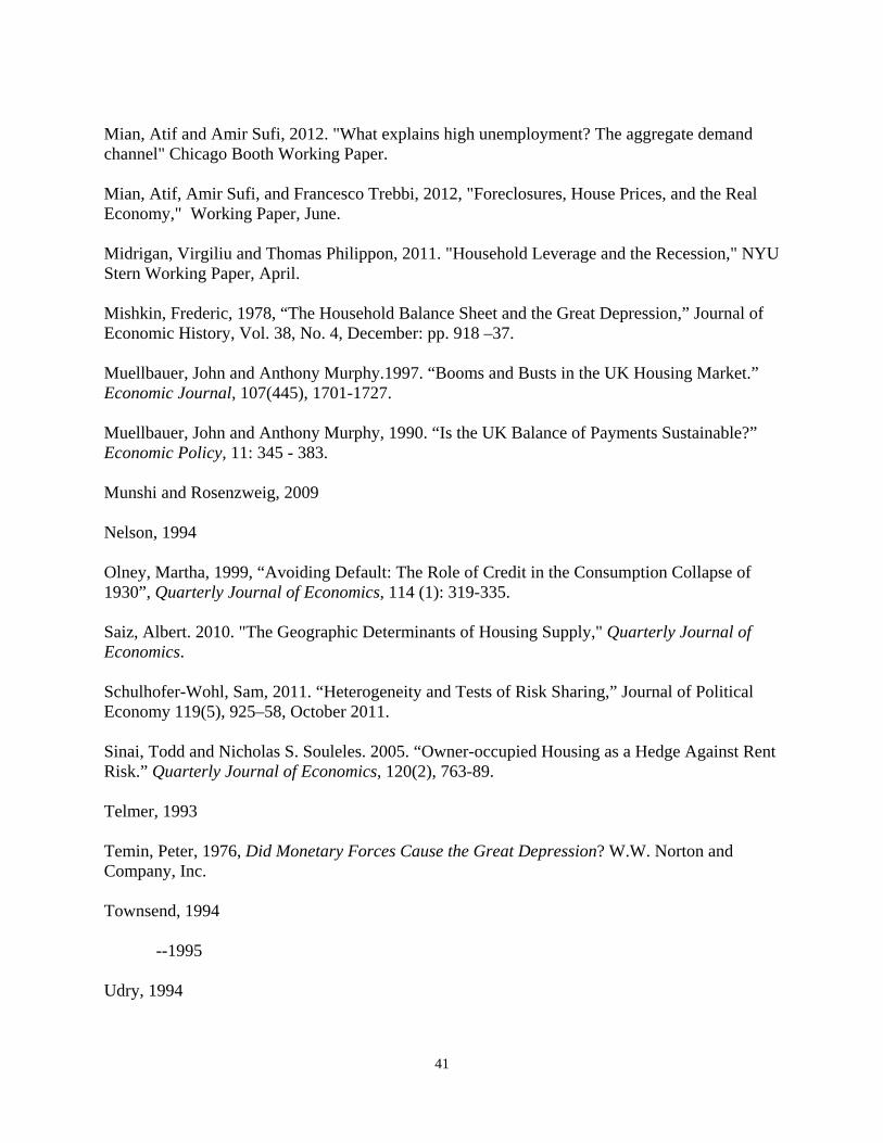
41  

Mian, Atif and Amir Sufi, 2012. "What explains high unemployment? The aggregate demand channel" Chicago Booth Working Paper. Mian, Atif, Amir Sufi, and Francesco Trebbi, 2012, "Foreclosures, House Prices, and the Real Economy," Working Paper, June. Midrigan, Virgiliu and Thomas Philippon, 2011. "Household Leverage and the Recession," NYU Stern Working Paper, April. Mishkin, Frederic, 1978, “The Household Balance Sheet and the Great Depression,” Journal of Economic History, Vol. 38, No. 4, December: pp. 918 –37. Muellbauer, John and Anthony Murphy.1997. “Booms and Busts in the UK Housing Market.” Economic Journal, 107(445), 1701-1727. Muellbauer, John and Anthony Murphy, 1990. “Is the UK Balance of Payments Sustainable?” Economic Policy, 11: 345 - 383. Munshi and Rosenzweig, 2009 Nelson, 1994 Olney, Martha, 1999, “Avoiding Default: The Role of Credit in the Consumption Collapse of 1930”, Quarterly Journal of Economics, 114 (1): 319-335. Saiz, Albert. 2010. "The Geographic Determinants of Housing Supply," Quarterly Journal of Economics. Schulhofer-Wohl, Sam, 2011. “Heterogeneity and Tests of Risk Sharing,” Journal of Political Economy 119(5), 925–58, October 2011. Sinai, Todd and Nicholas S. Souleles. 2005. “Owner-occupied Housing as a Hedge Against Rent Risk.” Quarterly Journal of Economics, 120(2), 763-89. Telmer, 1993 Temin, Peter, 1976, Did Monetary Forces Cause the Great Depression? W.W. Norton and Company, Inc. Townsend, 1994 --1995 Udry, 1994

42  

Zhou, Xia and Christopher Carroll, 2012, "Dynamics of Wealth and Consumption: New and Improved Measures for U.S. States," B.E. Journal of Macroeconomic Advances, 12: 4, 1-42

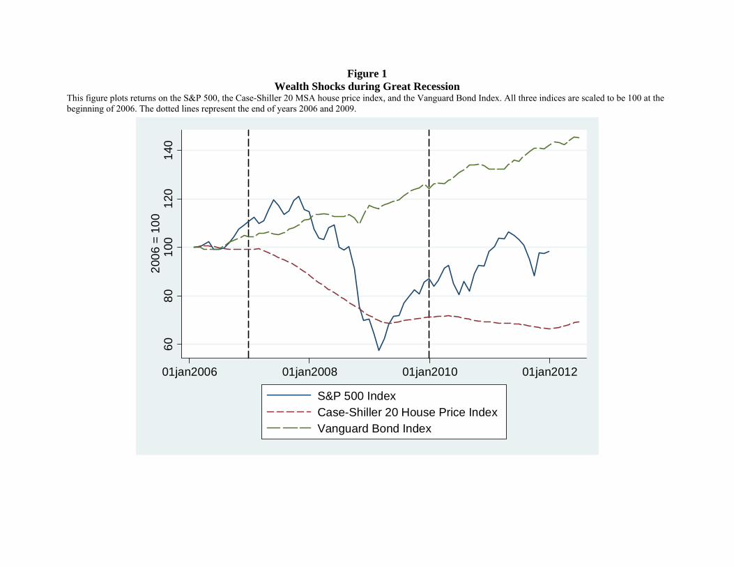
Figure 1 Wealth Shocks during Great Recession

This figure plots returns on the S&P 500, the Case-Shiller 20 MSA house price index, and the Vanguard Bond Index. All three indices are scaled to be 100 at the beginning of 2006. The dotted lines represent the end of years 2006 and 2009.

6080

100

120

140

2006

= 1

00

01jan2006 01jan2008 01jan2010 01jan2012

S&P 500 IndexCase-Shiller 20 House Price IndexVanguard Bond Index

Figure 2 House Prices, Leverage Multiplier, and Housing Net Worth Shock

The left panel plots the zip code level correlation between the two components of the housing net worth shock: house price growth from 2006 to 2009 and the leverage multiplier. The leverage multiplier is 1/(1-LTV) where LTV is calculated as the (debt-financial assets)/housing assets. The housing net worth shock reflects the growth in total net worth due to the growth in housing net worth. It is equivalently the leverage multiplier times the growth in house prices. The right panel sorts zip codes into deciles by the housing net worth shock (weighted by population), and shows each decile's net worth shock.

-.8-.6

-.4-.2

0.2

Hou

se p

rice

grow

th 2

006-

2009

-.2 0 .2 .4 .6 .8 1 1.2 1.4Leverage multiplier

Correlation between house price shock and leverage

-.5-.4

-.3-.2

-.10

Hou

sing

net

wor

th s

hock

, 200

6-20

09

1 2 3 4 5 6 7 8 9 10

Distribution of housing net worth shock by decile

Figure 3 Housing Supply Elasticity as a Source of Variation for Housing Net Worth Shock

The three panels plot the relation between housing supply elasticity and house price growth from 2006 to 2009 (upper-left panel), the leverage multiplier in 2006 (upper-right panel) and the growth in housing net worth between 2006-2009 (lower-left panel) vary with housing supply elasticity instrument. The leverage multiplier is 1/(1-LTV) where LTV is calculated as the (debt-financial assets)/housing assets. The housing net worth shock reflects the growth in total net worth due to the growth in housing net worth. It is equivalently the leverage multiplier times the growth in house prices. A unit of observation is CBSA and each observation is weighted by it population (number of households).

-.8-.6

-.4-.2

0H

ouse

pric

e ch

ange

, 200

6-20

09

.5 1 1.5 2 2.5 3 3.5 4Housing supply elasticity

.2.4

.6.8

1Le

vera

ge M

ultip

lier,

2006

.5 1 1.5 2 2.5 3 3.5 4Housing supply elasticity

-.6-.4

-.20

Hou

sing

net

wor

th s

hock

, 200

6-20

09

.5 1 1.5 2 2.5 3 3.5 4Housing supply elasticity

Figure 4 Elasticity of Spending with Respect to Housing Net Worth Shock

The scatter-plot relates total spending growth in a county from 2006 to 2009 to the housing wealth shock over the same time period. The housing net worth shock reflects the growth in total net worth due to the growth in housing net worth. It is equivalently the leverage multiplier times the growth in house prices. The scatter-plot and regression line are weighted by total population of the county.

-.6-.4

-.20

.2.4

Gro

wth

in s

pend

ing,

200

6-20

09

-.6 -.4 -.2 0Housing net worth shock, 2006-2009

Figure 5 Credit Tightening and Housing Net Worth Shock

These scatter plots relate credit tightening with the housing net worth shock. The credit tightening variable represents the first principal component of the decline in home equity limits, the decline in credit card limits, and the increase in the home equity and credit card utilization rates. The housing net worth shock reflects the growth in total net worth due to the growth in housing net worth. It is equivalently the leverage multiplier times the growth in house prices. The scatter-plot and regression line are weighted by total population of the county.

-.4-.2

0.2

.4C

redi

t tig

hten

ing

from

200

6 to

200

9

-.7 -.6 -.5 -.4 -.3 -.2 -.1 0 .1Housing net worth shock, 2006-2009

Figure 6 The Average Marginal Propensity to Consume

The left-panel scatter-plot relates the change in total spending per household in a county from 2006 to 2009 to the change in home values over the same time period. The scatter-plot and regression line are weighted by total population of the county. The gradient of the red line represents the average marginal propensity to consume. The right panel plots the marginal propensity to consume for various spending categories.

-20

-10

010

Cha

nge

in s

pend

ing

per h

ouse

hold

, $ th

ousa

nds

-200 -150 -100 -50 0Change in home value per household, $ thousands

Marginal propensity to consume out of housing

0.054

0.023

0.016

0.011

0.004

0.0

2.0

4.0

6m

argi

nal p

rope

nsity

to c

onsu

me

total

auto

non-durables

other durables

groceries

MPC by type of spending

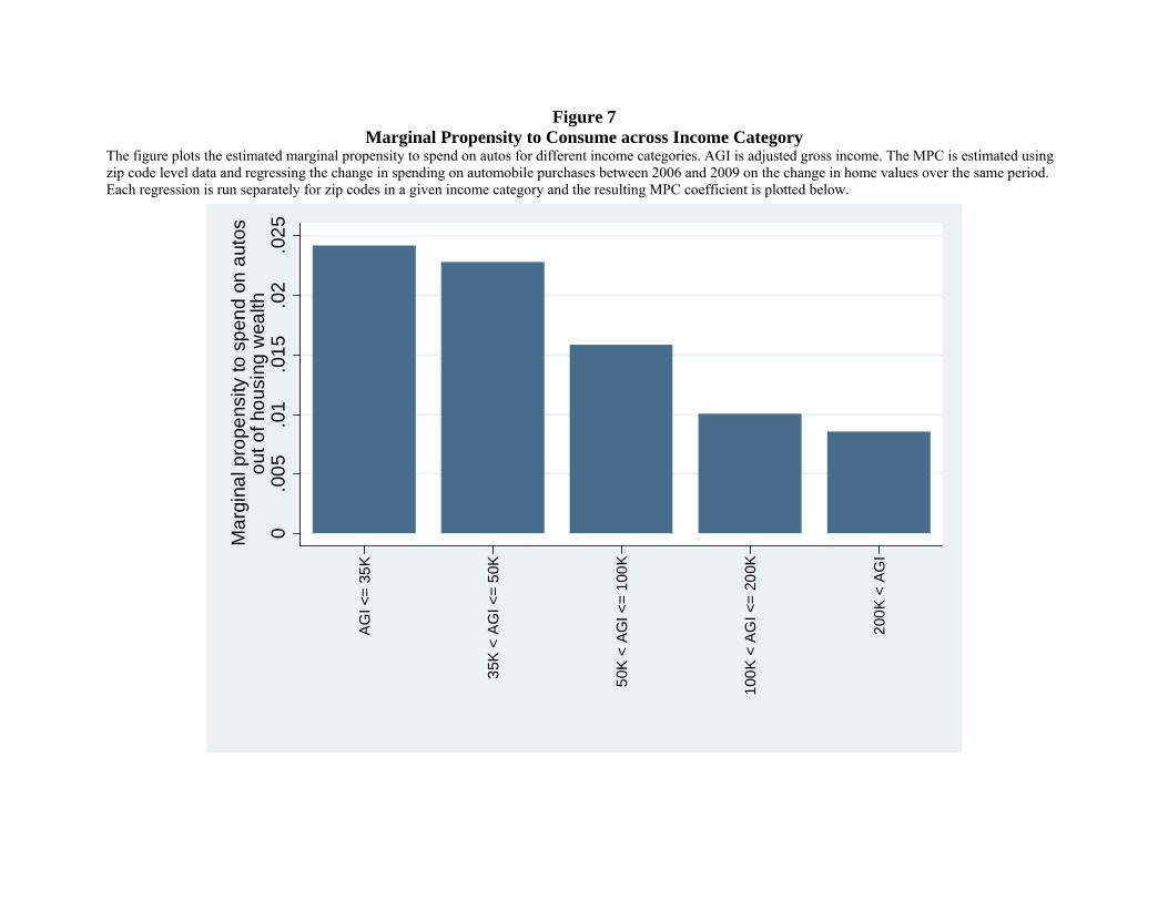
Figure 7 Marginal Propensity to Consume across Income Category

The figure plots the estimated marginal propensity to spend on autos for different income categories. AGI is adjusted gross income. The MPC is estimated using zip code level data and regressing the change in spending on automobile purchases between 2006 and 2009 on the change in home values over the same period. Each regression is run separately for zip codes in a given income category and the resulting MPC coefficient is plotted below.

0.0

05.0

1.0

15.0

2.0

25

Mar

gina

l pro

pens

ity to

spe

nd o

n au

tos

out o

f hou

sing

wea

lth

AG

I <=

35K

35K

< A

GI <

= 50

K

50K

< A

GI <

= 10

0K

100K

< A

GI <

= 20

0K

200K

< A

GI

Figure 8 Marginal Propensity to Consume by Underwater Homeowner Fraction

The figure plots the estimated marginal propensity to spend on autos based on the fraction of homeowners underwater on their mortgage as of 2011. So for example, the column on the far right gives the MPC for households in zip codes where more than 50% of homeowners are underwater. The MPC is estimated using zip code level data and regressing the change in spending on automobile purchases between 2006 and 2009 on the change in home values over the same period. Each regression is run separately for zip codes in a given underwater fraction category and the resulting MPC coefficient is plotted below.

0.0

05.0

1.0

15.0

2.0

25

Mar

gina

l pro

pens

ity to

spe

nd o

n au

tos

out o

f hou

sing

wea

lth

UW

<=

15%

15%

< U

W <

= 25

%

25%

< U

W <

= 40

%

40%

< U

W <

= 50

%

50%

< U

W

Table 1

Summary Statistics This table presents summary statistics for the counties in our sample. The sample is restricted to 944 counties for which we have data on the value of housing stock. These counties represent 82.1% of total U.S. population in 2006. The housing net worth shock reflects the growth in total net worth due to the growth in housing net worth. The financial net worth shock reflects growth in total net worth due to growth in financial net worth. The housing net worth shock and the financial net worth shock sum up to the growth in total net worth. Other durables include purchases at furniture, home appliance, and home center stores. Other non-durables include purchases at health, gasoline, clothing, hobby & sporting, and department stores. See the text for the corresponding NAICS codes.

N Mean SD 10th 90th Weighted

mean Weighted

SD Housing net worth shock, 2006-2009 944 -0.063 0.083 -0.169 0.003 -0.092 0.097 Financial net worth shock, 2006-2009 944 -0.096 0.011 -0.108 -0.084 -0.094 0.010 Change in home value, $000, 2006-2009 944 -28.4 38.4 -79.1 1.2 -47.5 49.1 Spending growth, 2006-2009 944 -0.059 0.135 -0.229 0.110 -0.092 0.113 Change in spending, $000, 2006-2009 944 -1.7 4.6 -6.7 3.3 -3.4 4.4 Change in auto spending, $000, 2006-2009 944 -2.6 1.6 -4.5 -1.0 -3.3 2.0 Change in other durables spending, $000, 06-09 944 -0.6 1.3 -2.0 0.5 -1.1 1.1 Change in grocery spending, $000, 2006-2009 944 0.5 0.9 -0.2 1.5 0.5 0.7 Change in other non-durable spending, $000, 06-09 944 1.0 2.8 -1.6 4.0 0.5 2.4 Employment share in construction, 2006 944 0.119 0.054 0.065 0.182 0.125 0.048 Employment share in tradables, 2006 944 0.130 0.102 0.032 0.247 0.110 0.071 Employment share in other, 2006 944 0.522 0.232 0.274 0.830 0.667 0.268 Employment share in non-tradables, 2006 944 0.210 0.067 0.137 0.283 0.216 0.051 Income per household, $000, 2006 944 52.2 15.9 38.2 70.2 59.9 18.9 Net worth per household, $000, 2006 944 429.9 246.7 230.5 684.5 520.8 288.8 Housing supply elasticity, Saiz 540 2.192 1.044 0.943 3.589 1.715 0.968 Number of households, thousands 944 98.2 187.5 12.8 237.8 455.9 666.2 Home equity limit growth, 2006-2009 944 -0.023 0.193 -0.214 0.165 -0.029 0.132 Credit card limit growth, 2006-2009 944 -0.037 0.082 -0.134 0.063 -0.050 0.056 Change in fraction of subprime borrowers , 06-09 944 -0.010 0.024 -0.038 0.019 -0.004 0.024 Refinancing loan growth, 2006-2009 944 0.221 0.596 -0.542 0.833 -0.031 0.705

Table 2 Correlation Matrix for Housing Net Worth Shock, Credit Market Shock, and Consumption Growth

This table presents pair-wise correlations between different variables. Panel A reports various components of the net worth shock experienced by households in a county between 2006 and 2009. Panel B reports correlation between changes in various credit market variables between 2006 and 2009. “CC factor” stands for credit constrained factor, which represents the first principal component of the first four variables (i.e. negative of the change in home equity limit, negative of the change in credit card limit, change in home equity utilization rate and change in credit card utilization rate). Under 660 represents the percentage of population in a county with a credit score below 660 in 2006. Panel C reports the change in various components of consumption between 2006 and 2009. The leverage multiplier is 1/(1-LTV) where LTV is calculated as the (debt-financial assets)/housing assets. The housing net worth shock reflects the growth in total net worth due to the growth in housing net worth. It is equivalently the leverage multiplier times the growth in house prices. The financial net worth shock reflects growth in total net worth due to growth in financial net worth. The housing net worth shock and the financial net worth shock sum up to the growth in total net worth. Throughout, ∆ implies natural logarithm differences. All pairwise correlations are significant at the 1% level, except for the correlation between Under 660 and change in credit card utilization rate, and Under 660 and the CC factor. Both these correlations are not significant even at the 10% level.

Panel A: Change in Consumption ∆Auto sales ∆Other durables ∆Other non-durables ∆Auto sales 1.000 ∆Other durables 0.414 1.000 ∆Other non-durables 0.267 0.382 1.000 ∆Groceries 0.202 0.493 0.541

Panel B: Credit Market Shocks -∆Home eq. limit -∆Credit card limit Change in home eq.

util. Change in credit card

util. CC factor

-∆Home eq. limit 1.000 -∆Credit card limit 0.336 1.000 Change in home eq. util. 0.236 0.111 1.000 Change in credit card util. 0.270 0.223 0.505 1.000 CC factor 0.912 0.574 0.501 0.485 1.000 Under 660, 2006 0.090 0.076 -0.197 0.046 0.043

Panel C: Net Worth Shocks Housing net worth

shock Financial net worth

shock Leverage Multiplier

Housing net worth shock 1.000 Financial net worth shock -0.327 1.000 Leverage Multiplier -0.706 0.554 1.000 ∆House Prices 0.898 -0.246 -0.451

Table 3 Housing Supply Elasticity as an Instrument

This table presents coefficients from regressions relating house price growth, the leverage multiplier and the housing net worth shock to the housing supply instrument. The unit of observation is a county. The leverage multiplier is 1/(1-LTV) where LTV is calculated as (debt-financial assets)/housing assets. The housing net worth shock reflects the growth in total net worth due to the growth in housing net worth. It is equivalently the leverage multiplier times the growth in house prices. Standard errors are heteroskedasticity robust, clustered at the state level. All regressions are weighted by total population. (1) (2) (3) (4) (5) (6) Dependent variable: House price growth 06-09 Leverage multiplier Housing net worth shock, 06-09 Elasticity 0.091** 0.169** -0.065** -0.145** 0.046** 0.097** (0.022) (0.056) (0.016) (0.042) (0.011) (0.023) Elasticity Squared -0.017 0.018** -0.011** (0.009) (0.007) (0.004) Constant -0.395** -0.461** 0.459** 0.527** -0.174** -0.217** (0.071) (0.087) (0.045) (0.060) (0.037) (0.041) N 540 540 540 540 540 540 R2 0.193 0.206 0.224 0.255 0.190 0.211 **,* Coefficient statistically different than zero at the 1% and 5% confidence level, respectively

Table 4 Housing Supply Elasticity as a Source of Variation

This table presents coefficients from county-level univariate regressions regressing variables on the housing supply elasticity instrument. Each row is a separate regression. Standard errors are heteroskedasticity robust, clustered at the state level. All regressions are weighted by total population. Housing supply

elasticity Constant N R2

(1) Change in wage growth, (02-06) - (98-02) -0.002 -0.010 540 0.002

(0.004) (0.008) (2) Population growth, 2002 to 2006 0.012* 0.018 538 0.026

(0.005) (0.012) (3) Units constructed per household, 02-06 0.014* 0.070** 540 0.032

(0.007) (0.016) (4) Employment share in construction, 2006 0.002 0.122** 540 0.003

(0.003) (0.008) (5) Construction employment growth, 02-06 0.005 0.940** 540 0.000

(0.015) (0.042) (6) Income per household, 2006 -5.378** 69.392** 540 0.080

(0.985) (2.191) (7) Net worth per household, 2006 -88.389** 674.620** 540 0.083

(20.689) (47.965) **,* Coefficient statistically different than zero at the 1% and 5% confidence level, respectively

Table 5 Net Worth Shock and Consumption Growth, 2006 to 2009

This table presents coefficients from regressions relating spending growth to the housing net worth shock. The unit of observation is a county. The housing net worth shock reflects the growth in total net worth due to the growth in housing net worth. The financial net worth shock reflects growth in total net worth due to growth in financial net worth. The housing net worth shock and the financial net worth shock sum up to the growth in total net worth. . Standard errors are heteroskedasticity robust, clustered at the state level. All regressions are weighted by total population. (1) (2) (3) (4) (5) (6) Dependent variable: Total spending growth, 2006 to 2009 IV State FE Excluding

AZ, CA, FL, NV

               Housing net worth shock, 2006-2009 0.634** 0.613** 0.590** 0.774** 0.457** 0.869** (0.125) (0.122) (0.130) (0.239) (0.101) (0.148) Financial net worth shock, 2006-2009 -0.595 (1.032) Construction employment share (2006) -0.448** -0.287 -0.171 -0.288 (0.150) (0.216) (0.127) (0.160) Tradable employment share (2006) 0.051 0.011 0.042 -0.027 (0.067) (0.092) (0.066) (0.065) Other employment share (2006) -0.025 -0.045 -0.057 -0.058 (0.038) (0.050) (0.037) (0.039) Non-tradable employment share (2006) 0.193 0.095 0.228 0.106 (0.157) (0.167) (0.137) (0.158) Ln(income per household, 2006) -0.002 0.024 -0.006 0.028 (0.033) (0.047) (0.046) (0.045) Ln(net worth per household, 2006) -0.028 -0.035 -0.023 -0.034 (0.018) (0.023) (0.020) (0.025) Constant -0.034* -0.092 0.167* 0.147 0.120 0.132 (0.015) (0.099) (0.077) (0.092) (0.090) (0.087) N 944 944 944 540 944 833 R2 0.298 0.301 0.355 0.319 0.547 0.230 **,* Coefficient statistically different than zero at the 1% and 5% confidence level, respectively

Table 6 Net Worth Shock and Credit Tightening, 2006 to 2009

This table presents coefficients from regressions relating credit tightening to the housing net worth shock. The unit of observation is a county. The housing net worth shock reflects the growth in total net worth due to the growth in housing net worth. The credit constraints factor represents the first principal component of the negative of the change in home equity limit, negative of the change in credit card limit, change in home equity utilization rate and change in credit card utilization rate. Standard errors are heteroskedasticity robust, clustered at the state level. All regressions are weighted by total population. (1) (2) (3) (4) (5) (6) Dependent variable: Home equity

limit growth, 06-09

Credit card limit growth,

06-09

Credit constraints factor

Change in subprime

share, 06-09

Refinancing growth, 06-09

                 Housing net worth shock, 2006-2009 0.417** 0.149** -0.474** -0.482** -0.171** 5.488** (0.048) (0.028) (0.030) (0.027) (0.011) (0.645) Construction employment share (2006) 0.101 0.074* 0.295 (0.095) (0.030) (0.574) Tradable employment share (2006) 0.036 0.011 1.560** (0.063) (0.012) (0.488) Other employment share (2006) 0.028 -0.018** -0.234* (0.021) (0.006) (0.115) Non-tradable employment share (2006) 0.001 0.069* 2.451** (0.131) (0.028) (0.752) Ln(income per household, 2006) -0.001 0.010 0.930** (0.027) (0.006) (0.190) Ln(net worth per household, 2006) -0.006 0.007 -0.546** (0.021) (0.005) (0.162) Constant 0.010 -0.035** 0.019** 0.024 -0.115** -0.513 (0.012) (0.006) (0.006) (0.079) (0.018) (0.386) N 939 939 939 939 939 939 R2 0.106 0.072 0.258 0.268 0.695 0.778 **,* Coefficient statistically different than zero at the 1% and 5% confidence level, respectively

Table 7 Average Marginal Propensity to Consume out of Housing Wealth

This table presents coefficients from regressions relating the change in household spending to the change in home value between 2006 and 2009. Both the change variables are in thousands of dollars. All regressions are at the county level. Standard errors are heteroskedasticity robust, clustered at the state level. All regressions are weighted by total population. (1) (2) (3) (4) (5) (6) Dependent Variable Change in spending, $000

2006-2009

     

IV State FE Excluding AZ, CA, FL, NV      

Change in home value, $000, 2006-2009 0.054** 0.119** 0.051** 0.072** 0.051** 0.094** (0.009) (0.015) (0.011) (0.021) (0.013) (0.017) (Change in home value, $, 2006-2009)2 0.432** (0.076) Construction employment share, 2006 -9.748 -2.915 -7.449 -2.305 (5.479) (7.800) (5.379) (5.818) Tradable employment share, 2006 2.034 0.438 1.516 -0.795 (2.235) (3.783) (2.190) (2.496) Other employment share, 2006 -1.568 -3.037 -2.186 -2.629 (1.459) (1.850) (1.418) (1.466) Non-tradable employment share, 2006 -1.797 -3.256 -3.341 -4.106 (5.438) (5.983) (5.048) (5.349) Income per household, $000, 2006 -0.056* -0.019 -0.043 -0.022 (0.023) (0.032) (0.030) (0.029) Net worth per household, $000, 2006 0.003* 0.002 0.002 0.002 (0.001) (0.001) (0.002) (0.001) Constant -0.830 0.263 3.311** 3.211** 3.396** 3.415** (0.536) (0.554) (0.678) (0.928) (0.861) (0.837) N 944 944 944 540 944 833 R2 0.362 0.423 0.421 0.347 0.573 0.336 **,* Coefficient statistically different than zero at the 1% and 5% confidence level, respectively

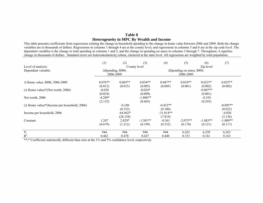
Table 8 Heterogeneity in MPC By Wealth and Income

This table presents coefficients from regressions relating the change in household spending to the change in home value between 2006 and 2009. Both the change variables are in thousands of dollars. Regressions in columns 1 through 4 are at the county level, and regressions in columns 5 and 6 are at the zip code level. The dependent variables is the change in total spending in columns 1 and 2, and the change in spending on autos in columns 3 through 7. Throughout, ∆ signifies change in thousands of dollars. Standard errors are heteroskedasticity robust, clustered at the state level. All regressions are weighted by total population. (1) (2) (3) (4) (5) (6) (7) Level of analysis: County level Zip level Dependent variable: ∆Spending, $000,

2006-2009 ∆Spending on autos, $000,

2006-2009

∆ Home value, $000, 2006-2009 0.076** 0.065** 0.034** 0.047** 0.018** 0.023** 0.025** (0.012) (0.015) (0.005) (0.005) (0.001) (0.002) (0.002) (∆ Home value)*(Net worth, 2006) -0.038 -0.024* -0.007** (0.024) (0.009) (0.001) Net worth, 2006 -4.289* -1.806** -0.354 (2.132) (0.665) (0.243) (∆ Home value)*(Income per household, 2006) -0.180 -0.432** -0.095** (0.332) (0.100) (0.022) Income per household, 2006 -64.042* -31.814** -4.020 (28.158) (7.819) (3.136) Constant 1.247 2.829* -1.301** -0.361 -2.075** -1.883** -1.809** (0.679) (1.212) (0.199) (0.332) (0.170) (0.121) (0.117) N 944 944 944 944 6,263 6,220 6,263 R2 0.462 0.478 0.427 0.440 0.153 0.161 0.163 **,* Coefficient statistically different than zero at the 1% and 5% confidence level, respectively

Table 9 Heterogeneity in MPC: The Role of Debt

This table presents coefficients from regressions relating the change in household spending to the change in home value between 2006 and 2009. Both the change variables are in thousands of dollars. All regressions are at the zip code level. The housing leverage ratio is defined to be the ratio of mortgage and home equity debt to home value in a zip code as of 2006. Throughout, ∆ signifies change in thousands of dollars. Standard errors are heteroskedasticity robust, clustered at the state level. All regressions are weighted by total population. (1) (2) (3) (4) (5) (6) (7) Level of analysis: Zip level Dependent variable: Housing leverage ratio,

2006 ∆Spending on autos, $000,

2006-2009 Fraction homeowners

underwater, 2011

∆ Home value, $000, 2006-2009 0.006** 0.010** 0.011** (0.002) (0.002) (0.002) (∆ Home value)*(Housing leverage ratio, 2006) 0.021** 0.020** 0.020** (0.003) (0.004) (0.003) Housing leverage ratio, 2006 -2.112** -2.146** -2.191** 0.041* 0.057** (0.228) (0.232) (0.230) (0.019) (0.019) (∆ Home value)*(Net worth, 2006) -0.005** (0.001) Net worth, 2006 0.004 -0.153 -0.141** (0.013) (0.158) (0.009) (∆ Home value)*(Income per household, 2006) -0.059** (0.015) Income per household, 2006 0.327 0.022 -1.583** (0.233) (1.627) (0.166) Constant 0.595** 0.576** -0.786** -0.667** -0.705** 0.387** 0.403** (0.011) (0.016) (0.150) (0.150) (0.157) (0.017) (0.018) N 6,385 6,448 6,222 6,182 6,222 6,055 6,115 R2 0.000 0.003 0.272 0.272 0.279 0.174 0.169 **,* Coefficient statistically different than zero at the 1% and 5% confidence level, respectively