households willingness to pay for soil...
TRANSCRIPT

HOUSEHOLDS’ WILLINGNESS TO PAY FOR SOIL
CONSERVATION PRACTICES IN ADWA WOREDA,
ETHIOPIA: A CONTINGENT VALUATION STUDY
GEBRELIBANOS GEBREMEDHIN GEBREMARIAM
BSc. (AgriEcon.), Haramaya University, Ethiopia
A THESIS SUBMITTED TO THE FACULTY OF
DEVELOPMENT STUDIES IN PARTIAL FULFILMENT FOR
THE REQUIREMENTS OF MASTERS OF SCIENCE DEGREE IN
AGRICULTURAL AND APPLIED ECONOMICS
UNIVERSITY OF MALAWI
BUNDA COLLEGE OF AGRICULTURE
DEPARTMENT OF AGRICULTURAL AND APPLIED
ECONOMICS
JULY 2012

i
DECLARATION
I, Gebrelibanos Gebremedhin Gebremariam, declare that this thesis is a result of
my own original effort and work, and that to the best of my knowledge, the findings
have never been previously presented to the University of Malawi or elsewhere for
the award of any academic qualification. Where assistance was sought, it has been
accordingly acknowledged.
Gebrelibanos Gebremedhin Gebremariam
Signature: _________________________
Date: ____________________________

ii
CERTIFICATE OF APPROVAL
We, the undersigned, certify that this thesis is a result of the authors‟ own work, and
that to the best of our knowledge, it has not been submitted for any academic
qualification within the University of Malawi or elsewhere. The thesis is acceptable in
form and content, and that satisfactory knowledge of the field covered by the thesis
was demonstrated by the candidate through oral examination held on 10th
July, 2012.
Major Supervisor: Abdi K. Edriss (Professor)
Signature: _________________________
Date: ____________________________
Co-Supervisor: Beston Maonga (PhD)
Signature: _________________________
Date: ____________________________

iii
DEDICATION
This thesis is affectionately dedicated to my grandparents.
iv
ACKNOWLEDGMENTS
I am deeply grateful and indebted to Professor Abdi K. Edriss, my major advisor, for
his guidance, supervision and suggestions. Successful accomplishment of this
research would have been very difficult without his generous time devotion from the
early design of the questionnaire to the final write up of the thesis by providing
valuable constructive comments and thus I am indebted to him for his kind and
tireless efforts that enabled me to finalize the study. My heart-felt thanks also go to
my co-advisor, Dr. Beston Maonga, for his scientific guidance, support and endless
concern in the course of the research. His assistance and inventive comments during
the write-up of the proposal for this study also deserve high appreciation. In short,
without the support of both my advisors this thesis would not have been as interesting
as it is now.
I also owe my deepest gratitude to Dr. MAR Phiri, Coordinator of CMAAE Program
at Bunda College and Department Head, for his help and guidance starting from
application to this program up to completion of my studies.
I would like to acknowledge African Economic Research Consortium (AERC) for
awarding me a scholarship throughout my study. I would also like to extend my
special thanks to the management staff of the AERC for their support, quick responses
and care throughout the programme.
I am also extremely grateful to Adwa Woreda administrators, agricultural experts and
farmers without whose help and cooperation this study would not have been

v
materialised. The enumerators also deserve special thanks for the effort they made to
collect reliable data.
In particular, I shall not forget the generosity and hospitality of staff members of the
Department of Agricultural and Applied Economics at Bunda College and at the
sheared facility for specialization and electives of University of Pretoria as well as my
fellow students. I want to say thank you all.
My deepest overwhelming acknowledgment goes for my uncle Dr. Amha
Gebremedhin and his family for their continuous moral and material support during
my course and research work.
I want to convey thanks to those persons who, directly or indirectly, have provided
support in my research work and whose names I may have forgotten to mention here.
Last but not least, I thank God for his wonderful mercies to enable me complete my
studies successfully.

vi
ABSTRACT
Soil erosion is one of the most serious environmental problems in the highlands of
Ethiopia. The prevalence of traditional agricultural land use and the absence of
appropriate resource management often result in the degradation of natural soil
fertility in the country. Hence, this study assesses farm households‟ WTP for soil
conservation practices through a CVM study. Double Bounded Dichotomous choice
with an Open ended follow up format was used to elicit the households‟ willingness to
pay. Based on data collected from 218 respondents, descriptive statistics indicated
that most of the respondents have perceived the problem of soil erosion and are
willing to pay for conservation practices. Probit model was employed to assess the
determinants of willingness to pay. Results of the model shows that age of the
household head, sex of the household head, education level of the household head,
family size, perception, land tenure, Total Livestock Units and initial bid were the
important variables in determining willingness to pay for soil conservation practices
in the study area. The study also show that the mean willingness to pay estimated
from the Double Bounded Dichotomous Choice and open ended formats was
computed at 56.65 and 48.94 person days per annum, respectively. The respective
total aggregate value of soil conservation in the study area (Adwa Woreda) was
computed to be 1,373,592 (16,483,104 Birr) and 1,186,648.18 (14,239,778.16 Birr)
per annum for five years, respectively. The results of the study have shown that socio
economic characteristics of the household and other institutional factors are
responsible for household‟s WTP for soil conservation practices. Therefore, policy
and program intervention designed to address soil erosion problems in the study area
have needed to take in to account these characteristics.

vii
TABLE OF CONTENTS
DECLARATION ............................................................................................................ i
CERTIFICATE OF APPROVAL .................................................................................. ii
DEDICATION ............................................................................................................. iii
ACKNOWLEDGMENTS ............................................................................................ iv
ABSTRACT .................................................................................................................. vi
LIST OF TABLES ........................................................................................................ xi
LIST OF FIGURES ..................................................................................................... xii
GLOSSARY OF ETHIOPIAN TERMS .................................................................... xiii
ACRONYMS .............................................................................................................. xiv
CHAPTER ONE ............................................................................................................ 1
1.0 INTRODUCTION .............................................................................................. 1
1.1 Background ..................................................................................................... 1
1.2 Statement of the Problem ................................................................................ 3
1.3 Justification of the Study ................................................................................. 4
1.4 Objective of the Study ..................................................................................... 6
1.5 Working Hypotheses ....................................................................................... 6
1.6 Research Questions ......................................................................................... 7
1.7 Organization of the Thesis .............................................................................. 7
viii
CHAPTER TWO ........................................................................................................... 8
2.0 REVIEW OF LITERATURE ............................................................................. 8
2.1 The Concept and Problem of Land Degradation ............................................. 8
2.2 Causes of Land Degradation ......................................................................... 10
2.3 Economic Values of Natural Resources ........................................................ 11
2.4 Natural Resources Valuation Methods .......................................................... 15
2.5 Theory of Welfare Economics ...................................................................... 16
2.6 Contingent Valuation Methods (CVM)......................................................... 20
2.6.1 Theoretical Literature............................................................................. 20
2.6.2 Bias Issues in Contingent Valuation Methods ....................................... 23
2.7 Empirical Studies .......................................................................................... 25
CHAPTER THREE ..................................................................................................... 31
3.0 METHODOLOGY ........................................................................................... 31
3.1 Sample and Sampling Technique .................................................................. 31
3.2 Data Source and Method of Data Collection ................................................ 32
3.3 Field Work Procedure and Questionnaire Design ......................................... 34
3.4 Method of Data Analysis............................................................................... 35
3.4.1 Theoretical Framework .......................................................................... 35
3.4.2 Empirical Model Specification .............................................................. 37
3.4.3 Estimation of the Mean Willingness to Pay ........................................... 40
3.5 Definition of Variables .................................................................................. 45

ix
CHAPTER FOUR ........................................................................................................ 51
4.0 RESULTS AND DISCUSION ......................................................................... 51
4.1 Descriptive Statistics ..................................................................................... 51
4.1.1 Summary of Households‟ Characteristics .............................................. 51
4.1.2 Resources Ownership............................................................................. 55
4.1.3 Physical Characteristics of Households Farm Land .............................. 56
4.1.4 Perception of Soil Erosion Hazard ......................................................... 58
4.1.5 Land Tenure ........................................................................................... 59
4.1.6 Labor Availability .................................................................................. 60
4.2 Analysis of Determinants of Households‟ WTP ........................................... 60
4.3 Households Willingness to Pay for Soil Conservation Practices .................. 70
4.3.1 Descriptive Statistics of the Discrete Responses ......................................... 70
4.2.2 Estimation of Mean from Double Bounded Dichotomous Choice Format . 72
4.3.1 Analysis of Results of the Open Ended Format ..................................... 74
4.3.2 Reasons for Maximum Willingness to pay ............................................ 76
4.4 Welfare Measure and Aggregation ............................................................... 78
CHAPTER FIVE ......................................................................................................... 81
5.0 CONCLUSION AND RECOMENDATION ................................................... 81
5.1 Conclusion ..................................................................................................... 81
5.2 Recommendation ........................................................................................... 84

x
REFERENCES ............................................................................................................ 87
APPENDIX I: Questionnaire ....................................................................................... 97
APPENDEX II: Contingent Valuation Scenario ..................................................... 108
APPENDIX III: Open Ended Question ..................................................................... 109
APPENDIX IV: VIF of Continuous Explanatory Variables ..................................... 109
APPENDIX V: Contingency Coefficient for Discrete Variables .............................. 109
xi
LIST OF TABLES
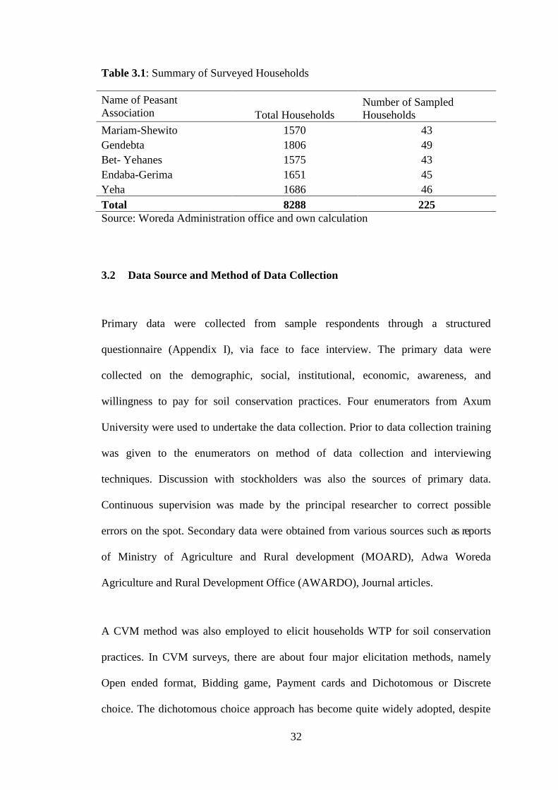
Table 3.1: Summary of Surveyed Households ............................................................ 32
Table 4.1: Sex Composition of Sample Households ................................................... 52
Table 4.2: Household Characteristics Marital Status and Social Position ................... 53
Table 4.3: Age, Family Size, Education and Distance to Market of Households........ 54
Table 4.4: Farm Size, Income and TLU Ownership of Sampled Households ............. 55
Table 4.5: Physical Characteristics of Households Farm Land ................................... 57
Table 4.6: Perception of Soil Erosion Hazard ............................................................. 58
Table 4.7: Land Tenure Security of Sampled Households .......................................... 59
Table 4.8: Labor Availability of Households .............................................................. 60
Table 4.9: Probit Model Estimates of WTP ................................................................. 62
Table 4.10: Marginal Effects of the Explanatory Variables ........................................ 67
Table 4.11: Summary of Discrete Responses to the Double- Bounded Questions ...... 71
Table 4.12: Frequency of Willingness to pay .............................................................. 72
Table 4.13: Descriptive Statistics of the Dichotomous Choice Format ....................... 72
Table 4.14: Estimates of the Double Bounded Dichotomous Choice Format ............. 73
Table 4.15: Willingness to Pay of Households Based on the Open Ended Format ..... 74
Table 4.16: Frequency Distribution of the Open Ended Questionnaire Format .......... 75
Table 4.17: Reasons for Maximum Willingness to Pay .............................................. 76
Table 4.18: Reasons for Not Willing to Pay ................................................................ 77
Table 4.19: Welfare Measures and Aggregate Benefits by Peasant Associations ....... 78

xii
LIST OF FIGURES
Figure 2.1: Components of TEV of Soil Resource ...................................................... 14
Figure 4.1: Ferequency Curve for Soil Conservation .................................................. 76

xiii
GLOSSARY OF ETHIOPIAN TERMS
Birr Is the local currency of Ethiopia
Kebele Is the lowest administrative unit in Ethiopia.
Tsimdi Is a measure of cultivable land (1 tsimdi = 0.25 hectare)
Woreda Is an administrative unit in rural Ethiopia which often used
interchangeably with District. It is the unit above kebele
administration.
Zone Is an administrative unit in Ethiopia, which is below the
level of regional state and above Woreda.
xiv
ACRONYMS
AERC African Economic Research Consortium
AWARDO Adwa Woreda Agricultural and Rural Development Office
CAM Conjoint Analysis Method
CEM Choice Experiment Method
CFW Cash for Work
CIM Cost of Illness Method
CV Compensating Variation
CVM Contingent Valuation Method
CS Compensating Surplus
DC Dichotomous Choice
EC Ethiopian Calendar
EHRS Ethiopian Highland Reclamation Study
EV Equivalent Variation
ES Equivalent Surplus
FFW Food for Work
GDP Gross Domestic Product
Ha Hectare
xv
HPM Hedonic Pricing Method
IFPRI International Food Policy Research Institute
MOARD Ministry of Agriculture and Rural Development
MPM Market Price Method
NFIM Net Factor Income Method
NGO None Governmental Organizations
PA Peasant Associations
PFM Production Function Method
RCM Replacement Cost Method
SMNP Simen Mountains National Park
TCM Travel Cost Method
TEV Total Economic Value
TLU Total Livestock Units
UN United Nation
USD United States Dollar
WTA Willingness to Accept
WTP Willingness to Pay

1
CHAPTER ONE
1.0 INTRODUCTION
1.1 Background
The economic development of developing countries depends on the performance of
the agricultural sector, and the contribution of this sector depends on how the natural
resources are managed. Unfortunately, in the majority of developing nations, the
quality and quantity of natural resources are decreasing resulting in more severe
droughts and floods (Fikru, 2009).
Ethiopia, being among these developing countries, has heavily relied on its
environmental and agricultural resource base for the past years. In general,
agriculture in the country is characterized by limited use of external inputs and
continuous deterioration of the resources. According to Daniel (2002), Ethiopia for
the last couple of decades has faced serious ecological imbalances because of large
scale deforestation and soil erosion caused by improper farming practices, destructive
forest exploitation, wild fire and uncontrolled grazing practices. This has resulted in a
declining agricultural production, water depletion, disturbed hydrological conditions,
and poverty and food insecurity.
Bojo and Cassells (1995), assessed land degradation and indicated that the immediate
gross financial losses due to land degradation in the Ethiopian highlands were about
USD 102 million per annum which was about 3 % of the country‟s GDP. The study
also showed that virtually all of the losses were due to nutrient losses resulting from

2
the removal of dung and crop residues from cropland, while the remaining was mainly
due to soil erosion. Other modeling work suggests that the loss of agricultural value
between 2000 and 2010 to be a huge about $7 billion (Berry, 2003).
Natural and environmental resources conservation in Ethiopia, specifically soil, is
therefore not only closely related to the improvement and conservation of ecological
environment, but also to the sustainable development of its agricultural sector and its
economy at large. According to Alemneh (2003), there was no Government policy on
soil conservation or natural resources management in Ethiopia prior to 1974. The
1974-1975 famine was the turning point in Ethiopian history in terms of establishing a
linkage between degradation of natural resources and famine. Since then, different
soil conserving technologies with a varied approach has been underway.
However, the achievements of those soil conservation attempts have been daunting. In
order to combat soil degradation and to introduce sustainable use of resources, there is
a need to take action. Thus, it is imperative that the local people participate in the
designing and practices of conservation measures. This study was undertaken in
Adwa at the Tigrian highlands of Ethiopia. At present, the study area is faced with
extreme soil degradation. The principal factors responsible for the problem include
steep topography, inherent erodible nature of the soils and expansion of farmland. The
study was aimed at identifying the factors that determine farmers‟ willingness to take
part in soil conservation practices.

3
1.2 Statement of the Problem
Soil is the second most important to life next to water. From the record of past
achievements, history tells us that civilization and fertility of soils are closely
interlinked. The declination of the fertility of soils had occurred due to accelerated
erosion caused by human interference. Today soil erosion is almost universally
recognized as a serious threat to human wellbeing.
Soil erosion is one of the most serious environmental problems in the highlands of
Ethiopia. The prevalence of traditional agricultural land use and the absence of
appropriate resource management often result in the degradation of natural soil
fertility. This has important implications for soil productivity, household food
security, and poverty in those areas of the country (Teklewold and Kohlin, 2011).
Serious soil erosion is estimated to have affected 25% of the area of the highlands and
now seriously eroded that they will not be economically productive again in the
foreseeable future (Hans-Joachim et al., 1996 as it is cited in Yitayal, 2004). The
average annual rate of soil loss in the country is estimated to be 42 tons/hectare/year
which results to 1 to 2% of crop loss (Hurni, 1993), and it can be even higher on steep
slopes and on places where the vegetation cover is low. This makes the issue of soil
conservation not only necessary but also a vital concern if the country wants to
achieve sustainable development of its agricultural sector and its economy at large.
Anemut (2006), argues that, natural resources such as soil are important natural
resources as they have useful effects on ecological balances and also for they are the
means for the livelihood of many local people worldwide; especially in the
developing countries. However, due to lack of efficient property right, increased

4
population growth, lower productivity of agriculture and fast expansion of farmlands
in most developing countries many environmentally important areas are highly
degraded. According to the same author, the non-participatory nature of
environmental policies, which gives less priority to the local communities need and
priorities in the management and use of natural resources, has worsened the problem
of natural resource degradation in most developing countries.
According to Wegayehu (2003), among the various forms of land degradation, soil
erosion is the most important and an ominous threat to the food security and
development prospects of Ethiopia and many other developing countries. It induces
on-site costs to individual farmers, and off-site costs to society. That coupled with
poverty, fast growing population and policy failure; poses a serious threat to national
and household food security.
To avert the global as well as local environmental disaster being brought by soil
erosion, it is imperative to take action quickly and on a vast scale. It is therefore, very
necessary to induce in every one‟s mind the importance of conserving soil resources.
Hence, in this study, an attempt was made to estimate local peoples‟ willingness to
pay for conservation practices.
1.3 Justification of the Study
The achievements of the soil conservation practices that have been undertaken in
Ethiopia have fallen far below expectations. The country still loses a tremendous
amount of fertile topsoil, and the threat of land degradation is broadening alarmingly
(Tekelu and Gezeahegn, 2003). This is mainly because; farmers‟ perception of their
5
environment has been misunderstood partly in the country. It is misunderstood partly
because outsiders, both scholars and policy makers, who write about farmers and
formulate polices, often have limited understanding about the farmers‟ attitude
towards environment. Furthermore, the farmers‟ view of the environment is often
ignored without due consideration of the condition he/she faces between survival and
environmental exploitation (Alemneh, 1990). So far, conservation practices were
mainly undertaken in a campaign often without the involvement of the land user
(Shiferaw and Holden, 1998).
Does such an experience mean that there is no hope for soil conservation in Ethiopia?
Absolutely not, the problem would have been rather, the projects that have been
undertaken in Ethiopia for soil conservation have failed to consider local peoples‟
willingness to pay for such projects from the very initiation of conservation measures.
This motivates that, there is a need to study on willingness to pay and design of
polices and strategies that promote resource conserving land use with active
participation of local people.
Thus, this study analyzes the value that farmers‟ attach to soil conservation practices,
determinants of their willingness to pay for soil conservation via labour contribution
and the welfare gain from such activities. Generally, understanding the factors leading
to willingness to pay in soil conservation practices would help policy makers to
design and implement more effective soil conservation plans.
6
1.4 Objective of the Study
The general objective of this study was to generate the demand side information from
households who are the major victims of land degradation and soil erosion. So, the
prime concern of this study is to elicit farmers‟ willingness to participate in soil
conservation and rehabilitation practices in the study area.
The specific objectives of the study were:
To identify the determinants that affects the willingness of households to
participate for soil conservation practices.
To estimate the mean labour contribution of households for soil conservation in
the study area.
To estimate the welfare gain of soil conservation project in the study area.
1.5 Working Hypotheses
With market imperfections, the probability or the level of farm household‟s WTP for
soil conservation depends on various factors, such as poverty and household
characteristics, than only farm characteristics. If markets (for example, credit markets)
were perfect, then farm households‟ WTP would depend only on farm characteristics
as they could address cash liquidity problems through these credit markets (Tessema
and Holden, 2006). Therefore, based on this theory the hypotheses are as follows:
1. Perception of severity of soil degradation at the study area will not affect the
household‟s WTP for soil conservation.

7
2. Socio economic variables such as age, sex, education level, social position of the
household head and land tenure do not affect households‟ willingness to pay for
soil conservation practices.
3. Wealth and resources endowments such as family size, total livestock holdings and
income of households do not affect willingness to pay of households‟ for soil
conservation practices.
1.6 Research Questions
The underline questions of this study were:
1. What is the value of soil conservation practices that the farmers attached to it?
2. What are the determinants of willingness to pay?
1.7 Organization of the Thesis
The forgoing Chapter has presented the introduction of the study. The rest of the
thesis is organized as follows. Chapter Two will present literature review. The
reviewed studies are in the area of soil and land degradation problems, natural
resources valuation methods and theory of welfare economics. Chapter Three
presents methodology. The Chapter starts with sample and sampling technique and
methods of data collection. Later the probit and bivariate probit models are discussed.
Results and discussions are presented in Chapter Four. Chapter Six concludes the
study and presents policy recommendations.

8
CHAPTER TWO
2.0 REVIEW OF LITERATURE
This chapter is mainly concerned with the review on soil and land degradation
problem in Ethiopia, natural resources valuation techniques and theory of welfare
economics. The chapter further reviews the criticisms of the contingent valuation
method. Finally, some studies that have been done in Ethiopia and elsewhere using
the contingent valuation method are reviewed.
2.1 The Concept and Problem of Land Degradation
Land degradation can be defined as a process that lowers the current and future
capacity of the land to support human life (Demeke, 1998). Land degradation and soil
degradation are often used interchangeably. However, land degradation has a broader
concept and refers to the degradation of soil, water, climate, and fauna and flora
(Alemneh et al. 1997 cited in Behailu, 2009).
Land/soil degradation can either be as a result of natural hazards or due to unsuitable
land use and inappropriate land management practices. Natural hazards include land
topography and climatic factors such as steep slopes, frequent floods and tornadoes,
blowing of high velocity wind, rains of high intensity, strong leaching in humid
regions and drought conditions in dry regions. Deforestation of fragile land, over
cutting of vegetation, shifting cultivation, overgrazing, unbalanced fertilizer use and
non-adoption of soil conservation management practices, over-pumping of ground
9
water (in excess of capacity for recharge) are some of the factors which comes under
human intervention resulting in soil erosion (Dominic, 2000).
Ethiopia is one of the Sub Saharan African countries where soil degradation has
reached a severe stage. Land degradation mainly due to soil erosion and nutrient
depletion, has become one of the most important environmental problems in the
country. Coupled with poverty, fast growing population and policy failures, land
degradation poses a serious threat to national and household food security (Shiferaw
and Holden, 1999). According to Gebreegziabher et al. (2006), in Ethiopia where
deforestation is a major problem, many peasants have switched from fuel wood to
dung for cooking and heating purposes, thereby damaging the agricultural
productivity of cropland. In Tigrai region, for example, dung rose from about 10% of
total household fuel consumption in the 1980s to about 50 percent by the year 1999.
An Ethiopian Highland Reclamation Study (EHRS) conducted two decades ago
revealed a frightening trend in environmental degradation where by “…27 million
hectares or almost 50% of the highland area was significantly eroded, 14 million
hectares seriously eroded and over 2 million hectares beyond reclamation. Erosion
rates were estimated at 130 tons/ha/yr for cropland and 35 tons/ha/yr average for all
land in the highlands….”. Forests in general have shrunk from covering 65% of the
country and 90% of the highlands to 2.2% and 5.6% respectively” With the country‟s
population now almost double what it was then, things have, obviously, gotten much
worse since (Aynalem, Undated).
10
2.2 Causes of Land Degradation
Land degradation is the result of complex interactions between physical,
environmental, biological, socio-economical, and political issues of local, country
wide or global nature. But, the major causes of land degradation are caused by the
mismanagement of land by the respective local uses.
The causes of land degradation can be grouped in to proximate and underlying
factors. The proximate causes of land degradation include cultivation of steep slopes
and erodible soils, low vegetation cover of the soil, burning of dung and crop
residues, declining fallow periods, and limited application of organic or inorganic
fertilizers. The underlying causes of land degradation include such factors as
population pressure; poverty; high costs or limited access of farmers to fertilizers, fuel
and animal feed; insecure land tenure; limited farmer knowledge of improved
integrated soil and water management measures; and limited or lack of access to
credit. The proximate causes of land degradation are the symptoms of inappropriate
land management practices as conditioned by the underlying factors. Hence, efforts
for soil conservation need to address the underlying causes primarily, as focusing on
the proximate causes would mean addressing the symptoms of the problem rather than
the real causes (Gebremedhin, 2004).
According to Hurni (1988), both environmental and socio-political factors have
contributed to the poor performance of Ethiopian agriculture. Environmental factors
include the dissected terrain, the cultivation of steeper slopes, erratic and erosive
rainfall, and so on. Socio-political factors include the top down approach adopted by
bodies intervening to improve soil and water conservation. Farmers have been

11
minimally involved in soil conservation activities and indigenous knowledge has been
undermined within planning, design, and implementation processes. As a result, soil
and water conservation programs have to date proved to be highly unpopular among
farmers.
In response, the government of Ethiopia attempted to combine incentives with
participatory approaches to soil conservation. However, real participation of
beneficiaries has not been realized in the country. Perhaps as a result, the adoption of
soil conservation practices remains low. Moreover, the use of indirect economic
incentives such as credit supply, extension services, reduction of land taxes, input and
output price support and market development has been limited. These experiences
indicates that there is a need to use both direct and indirect incentives combined with
real participation of beneficiaries if effective and sustained soil conservation effort is
to take place (Gebremedhin, 2004). This is due because there are no perfect markets
for soil erosion prevention practices as the good is public. Therefore, the objective of
this study is to determine the value that households attach to reduce soil and land
degradation in the study area, as manifested in their willingness to pay.
2.3 Economic Values of Natural Resources
For market prices to represent the correct value society attaches to the good, markets
need to be competitive and work freely. In such cases, prices are taken as an
expression of the willingness to pay for the good, which is the total value the buyer,
has for the good. But in reality markets are far from being perfect, and even they do
not exist for some class of goods. Therefore, to measure the value people attach to

12
goods, which do not have a perfect market, or any market at all; we need to
understand the concept of value (Aklilu, 2002).
This is at least for the following reasons. Firstly, there is a situation where markets are
missing to value the natural resources. In the absence of perfect markets, values of
goods and services are not properly revealed. Secondly, even if markets exist, they do
not do their job well due to market distortions, for example imperfect land property
rights in the study area could lead to land degradation, in this case. Thirdly,
uncertainty is involved about the demand and supply of natural resources and/or it is
difficult to estimate, especially in the future due to the non rival and excludability
nature of such resources. This is in the sense that, most economic markets capture, at
best, the current preferences of the buyers and sellers. Fourthly, governments may like
to use the valuation as against the restricted, administered or operating market prices
for designing natural resources conservation programmes. Fifthly, in order to arrive at
natural resource accounting, for methods such as Net Present Value methods, or for
cost-benefit analyses, valuation is a necessity. Finally, for most natural resources, it is
essential to understand and appreciate its alternatives uses apart from its direct value
of the resources such as existence and indirect values (Kadekodi, 2001).
The expression of total economic value bears as an attempt to overcome the
traditional evaluation of environmental goods, exclusively based on the use value
attributed to goods considering direct benefits enjoyed by final consumers. It seems
that the expression “total economic value” appeared for the first time in an essay by
Peterson and Sorg in 1987, “Toward the measurement of total economic value”. Then
the term was more and more used by other environmental economists.

13
The use value derives from a concrete use of environmental goods. Every use, in any
moment and by anyone is realized to create use values, which are more or less
measurable since they derive from their current use. Increase in crop production can
be considered as the use value of soil conservation.
But the total economic value is not only use value; it is given by the sum of use and
nonuse values referring to intrinsic benefits, i.e. those deriving from the mere
existence of environmental goods, in our case soil. The first economist, who identified
the total economic value double feature, was Kutrilla, (1995). After Kutrilla the
scholars interested in these topics have not been limited to theoretical analysis of the
total economic value and of its components, but their attention is centered on an
empirical analysis which allows them to identify the main features especially of non-
use value and the different methods usable for their measurement.
As shown in Figure 2.1 the Total Economic Value (TEV) that people attach to an
environmental good is the summation of use value and non-use value. Use value
refers to the benefit people get by making actual use of the good now or in the future.
Use value is divided into direct use value, indirect use value and option values.
Protection from soil erosion is a direct benefit that comes from better soil
management practices. By definition, use values derive from the actual use of the
environment while non-use values are non-instrumental values which are in the real
nature of the thing but unassociated with actual use, or the option to use the thing.
Instead such values are taken to be entities that reflect people‟s preferences, but
include concern for, sympathy with, and respect for the rights or welfare of non-
human beings. Soil resources can be also valued for their potential to be available in
the future. These potential future benefits constitute an option value. It may be

14
thought of as an insurance premium one may be willing to pay to ensure the supply of
the soil resources later in time.
The theoretical framework for total economic values of soil conservation is depicted
in Figure 2.1.
Source: Adopted from Hodge and Dunn 1992, cited in Marcouiller et al. (1999), with modifications
Figure 2.1: Components of TEV of Soil Resource
Total Economic
Value (TEV)
Non Use value
Use Value
Direct Use Value
Indirect Use
Value
Option
value
Bequest
value
Existence
Value
Direct uses of
soil,
consumption and
non
consumption
uses
Benefits
derived from
the
environmenta
l functions of
the soil
Future direct
and indirect
use values
Valued from
knowledge
of continued
existence
Value of
leaving use
and non
use values
for
offspring
Crops,
vegetables,
Animal
feed,
Fuel wood,
Recreation
Nutrient
retention,
Reduce
global
warming,
Waste
assimilation
Future
medicine,
Biodiversity
conservation
Habitats,
Endangered
species,
Biodiversity
Habitats,
Biodiversity
15
Non-use value is divided into existence and bequest value. Existence value is the
value people attach to soil conservation service not because they want to use the soil
now or in the future, but because they just want to make sure the soil exists. Bequest
value is a non-use value that one expects his/her descendents to get from the soil
conservation services.
2.4 Natural Resources Valuation Methods
Environmental valuation techniques help to estimate the value people attach to
environmental amenity or services, i.e., how much better or worse off individuals are
or would be as a result of a change in environmental quality. Since there are no
existing markets for environmental goods, people‟s valuation for these kinds of goods
could be elicited using two techniques. When a valuation technique considers related
or surrogate markets in which the environmental good is implicitly traded, it is
referred as a revealed preference method or indirect valuation method. Examples of
this valuation method include the travel cost method (TCM), the hedonic pricing
method (HPM), the production function method (PFM), the net factor income method
(NFIM), the replacement cost method (RCM), the market prices method (MPM), and
the cost-of-illness method (CIM). The second category of environmental resource
valuation methods is known as the stated preference method or direct valuation
method. These comprise survey-based methods that can be used either for those
environmental goods that are not traded in any market or for assessing individuals‟
stated behavior in a hypothetical setting. The method includes a number of different
approaches such as choice experiment method (CEM), contingent valuation method
(CVM) and conjoint analysis (CAM) (Aklilu, 2002; Tietmberg, 2003; Birol et al.,
2006 cited in Habtamu, 2009).
16
But for this study, only contingent valuation method was used to elicit the WTP of
households for soil conservation practices. One reason for using CVM is its
superiority over other valuation methods, which is its ability to capture, both use and
non-use values. Using other valuation methods such as hedonic pricing and travel cost
method would underestimate the benefits people get from soil conservation since they
measure use values only (Aklilu, 2002).
The other reason for using CVM is its ease of data collection and requirement
compared to other valuation methods. Further, the other methods such as TCM and
HPM are based on Marshallian demand which does not hold utility constant, which is
difficult to measure the change in welfare if utility does not hold constant. Therefore,
CVM is the best valuation method available for measuring the total value people give
for soil conservation in Adwa, Ethiopia.
2.5 Theory of Welfare Economics
The basic concept of welfare economics is that the purpose of any economic activity
is to increase the wellbeing of the responding individual or economic agent. In our
case, the basic assumption is that, individuals make decisions to maximize their utility
based on how well he or she is given situations and constraints. From this, it follows
that the basis for deriving measures of economic values is based on the effect of the
hypothesized project on respondent‟s wellbeing.
Welfare economics, whose theory relates to the basic theory of individual preferences
and demand for goods, seeks to make judgments about the desirability of having some
projects undertake to generate some benefits or payments of compensation not to do

17
projects (Alebel, 2002). Welfare economics can be measured by a cardinal utility
theory. However, a welfare measure based on the cardinal theory has drawbacks to
correctly measure the welfare change of a given project in the sense that it assumes
utility is measurable in a cardinal sense and comparable across individuals. According
to Alebel (2002), the notion of cardinal utility had been completely rejected in favour
of an ordinal definition of utility. This ordinal definition of utility enables consumers
to preferentially rank alternative bundles of goods in a manner consistent with certain
axioms of rational behaviour that include completeness, transitivity, convexity and
non-satiation.
The best way of explaining welfare is based on the Pareto criterion, which stated that
policy changes which make at least one person better off without making any one
worse off are desirable. According to Haab and McConnell (2002), the idea of a
potential Pareto improvement provides the rationale of public intervention to increase
the efficiency of resource allocation. That is, if the sum of the benefits from a public
action, to whomever they may occur, exceeds the costs of the action, it is deemed
worthwhile by this criterion.
This allows the calculation of net gain or loss from a policy change, and
determination of whether the change is potentially Pareto improving. The gains from
changes in environmental quality can be derived from the effects in individual‟s
welfare through changes in prices they pay for marketed goods, changes in prices they
receive for their factors of production, changes in the risks they face and changes in
the quantities or qualities of non-marketed goods or public goods such as
improvement in soil conservation, in this case.

18
Benefit can be measured using either the consumer surplus, the area under the
Marshalian demand curve, or one of the four which Hicks (1943) suggested;
compensating variation (CV), equivalent variation (EV), compensating surplus (CS)
and equivalent surplus (ES). Use of the Marshalian demand curve in stated preference
methodology is problematic because utility is not kept constant. That is, in Marshalian
demand analysis, the change in demand of the good to be valued due to a change in
price, is the sum of the income as well as substitution effects. The income effect is the
component of the total effect of a price change due to change in purchasing power.
The substitution effect is the component of the total effect of a price change due to the
change in the relative attractiveness of the good. This increase reflects a movement
along the same indifference curve. This shows that when someone is interested to
calculate the willingness to pay he has to remove the income effect, because the
willingness to pay estimates should reflect the substitution effect only, where the
individual utility level remains unchanged.
The limitation of the Marshalian demand of including both the income and
substitution effects due to a price change to estimate the willingness to pay can be
addressed by the Hicksian compensated demand. The Hicksian measures take only the
substitution effect, where the individual‟s utility levels are kept constant along the
compensated Hicksian demand curve. CV and CS are measures of the gains or loss
which hold utility constant at the initial level while EV and ES are measures of
welfare change which hold utility constant at some specified alternative level.
Policy interest usually lies in the potential benefits as measured from consumer‟s
current or initial level of utility. Furthermore, if the proposed change is welfare
increasing, which is the focus of this study, then the appropriate welfare measure is

19
the compensating surplus (Mitchell and Carson, 1989). This measure can be
interpreted as the consumer‟s maximum willingness to pay in order to gain the
quantity increase and still maintain his initial level of utility.
If one is interested to estimate the Hicksian demand curve in order to calculate the
benefit of policy change, he/she must correctly estimate the demand function for the
improvement of the public good. However, this task is difficult due to the fact that
estimation of demand requires substantial methodological efforts as well as due to
lack of accurate market data for these goods. An alternative method to this is to use a
hypothetical market model, which is a contingent valuation method, where
hypothetical questions on their willingness to pay for a particular effect are presented
to people. This method requires the creation of a market scenario that resembles
actual market situation for goods and services, which does not have efficient market
or no market at all. From the survey data obtained using contingent valuation method,
not only a maximum willingness to pay data can be generated, which will be used to
construct the demand curves but also used to conduct valuation process of the public
good without having to estimate the actual demand curve (Alebel, 2002).
The willingness to pay to improve the productivity of the land using the concept of
the Hicksian compensated surplus measure can be represented as follows (Holden and
Shiferaw, 2002).
)1.........(........................................).........,,,(),,,( 1000
hh ZKEUPeZKEUPeWTP
Where WTP is Hicksian compensating surplus, P is vector of prices, 0EU is the
current expected utility level, 0K is the old soil conservation technology, and 1K is the

20
new soil conservation technology that helps to maintain productivity, and hZ
represents farm and household characteristics as well as other exogenous variables
that affect the WTP. The function e(.) is an expenditure function that represents the
minimum expenditure level required to attain the initial level of utility 0EU before
and after the change. The WTP is therefore the difference in the level of expenditure
required to attain the initial level of utility after the change in the soil conservation.
The households will be willing to participate in soil conservation if they perceive that
the use of technology K1 (soil conservation structure) would help them to maintain the
productivity of their land, which otherwise would deteriorate due to erosion and other
land degradation factors. Inclusion of household characteristics is important here as
we are dealing not with pure consumers but with farm households who are both
producers and consumers of their produce. These are entities that operate in imperfect
market conditions, and their production and consumption decisions are not separable
(Tessema and Holden, 2006).
2.6 Contingent Valuation Methods (CVM)
2.6.1 Theoretical Literature
CVM is an environmental valuation method, which uses a hypothetical market to
appraise consumer preferences by directly asking their willingness to pay or
willingness to accept for change in the level of environmental good or services. The
contingent valuation method involves directly asking people, in a survey, how much
they would be willing to pay for specific environmental services. In some cases,
people are asked for the amount of compensation they would be willing to accept to
21
give up specific environmental services. It is called “contingent” valuation, because
people are asked to state their willingness to pay, contingent on a specific hypothetical
scenario and description of the environmental service.
If a researcher manages to correctly apply the procedures, CVM can able to capture
the total value of the good- both use and non-use values and its flexibility facilitates
valuation of a wide range of non-market goods. As a result, CVM is becoming the
most preferred valuation method at present (Mitchell and Carson, 1989; Whittington,
1998). Although economists were slow to adopt the general approach of CVM, the
method is now ubiquitous (Haab and McConnell, 2002).
In most CVM applications, the major steps are the following
Deciding what change you are going to value
Deciding how you are going to implement the questionnaire
Designing and administering the CVM survey
Analysis of the responses
Estimating and aggregating benefits (WTP)
Evaluating the CVM exercise (Validation Tests)
Contingent valuation survey consists three basic parts (Mitchell and Carson, 1989).
First, a hypothetical description of the condition under which the good or service is to
be offered as presented to the respondent. Second, questions which elicit the
respondents‟ willingness to pay for the goods being valued are presented. Finally,
questions on socio-economic, demographic characteristics and their use of the good or
service under consideration are given to the respondents.

22
A CVM study could be undertaken using different elicitation methods or method of
asking questions. This part of the questionnaire confronts the respondent with a given
monetary amount, and one way or the other induces a response. This has evolved
from the simple open-ended question of early studies such as „What is the maximum
amount you would pay for…..?‟ through bidding games and payment cards to
dichotomous choice questions Below, we have discussed the approaches of asking
questions that lead directly to willingness to pay or provide information to provide
preferences (Haab and McConnell, 2002).
Open Ended Format: A CVM question in which the respondent is asked to provide
the interviewer with a point estimate of his or her willingness to pay (ibid).
Bidding Games: This method starts by asking respondents whether they accept a
given price for the good and higher or lower prices will be offered depending on the
answer given to the initial prices. The bidding stops when iterations have converged
to a point estimate of willingness to pay (ibid).
Payment Cards: A CVM question format in which individuals are asked to choose a
willingness to pay point estimate (or a range of estimates) from a list of values
predetermined by the surveyors, and shown to the respondent on a card (ibid).
Dichotomous or Discrete Choice CVM: A CVM question format in which
respondents are asked simple yes or no questions of the stylized form: Would you be
willing to pay $t? (ibid)

23
As it is discussed earlier, a CVM study could be undertaken using one of the above
methods. But the first three methods have been shown to suffer from compatibility
problems in which survey respondents can influence potential outcome by revealing
values other than their true willingness to pay. The dichotomous choice approach has
become quite widely adopted, despite criticisms and doubts, in parts because it
appears to be incentive compatible in theory. When respondents do not give a direct
estimate of their willingness to pay, they have diminished ability to influence the
aggregate outcome. However, this advantage of compatibility has a limitation.
Estimates of willingness to pay are not revealed by respondents (Haab and
McConnell, 2002). To improve the precision of the WTP estimates, in recent years
researchers have introduced a follow up question to the dichotomous question
(Alberini and Cooper, 2000). Hence, in this study, a double bounded dichotomous
question and an open ended follow up was used. This approach is similar to real life
situation in Ethiopia at a market where the seller first states some bid price for a good
and then negotiation starts between the seller and the buyer. Some studies (for
instance, Alemu, 2000; Paulos, 2002; Anemut; 2006, Habtamu, 2009) implement an
elicitation procedure, which includes an initial dichotomous choice payment question
followed by another question.
2.6.2 Bias Issues in Contingent Valuation Methods
Although CVM is the best method for valuing non marketed goods, it has some
limitations. One of the main limitations of a CVM study is that due to the hypothetical
nature of the good which is going to be valued. This relates to the fact that, many
people have little experience in making explicit value of the environmental good
especially the non use values. Therefore, some people have difficulties to accept

24
results obtained through CVM as true willingness to pay which will be revealed if the
good valued were to be supplied in reality. But many studies have shown that CVM
can give a reliable result if applied correctly and carefully (Whittington, 1998;
Alberini and Cooper, 2000).
The other main limitation of a CVM study is that, it looks only at the demand side of
the public good. It is argued that as an expressed-preference valuation method, CVM
is inherently susceptible to various types of bias. Biases can be broadly classified into:
general (strategic) and instrument (starting point bias). The designer of CVM study
should, therefore, take these possible biases into consideration (Paulos, 2002). Some
of the biases in CVM study are discussed below.
Starting point bias: This is a bias that occurs when the respondent‟s willingness to
pay is influenced by the initial value suggested to the respondent to take it or leave it.
This problem is encountered when the elicitation format involves starting values.
Hypothetical bias- The unique future of CVM is its hypothetical nature of the good
and hence could be suffered from hypothetical bias. If respondents are not familiar
with the scenario presented, their response cannot be taken as their real willingness to
pay. This bias can be minimized by a careful description of the good under
consideration for the respondents.
Compliance bias–occurs when the interviewer is leading the respondent towards the
answer he/she is expecting. Compliance bias can also come because of the sponsor of
the good being valued. This bias can be reduced by carefully designing the survey,

25
good training of the interviewers and good supervision of the main survey (Mitchell
and Carson, 1989).
Strategic bias –arises when the respondents expect something out of the result of the
study and report not their real WTP/WTA but something which they think will affect
the research outcome in favour of them. Respondents may tend to understate their true
willingness to pay if they think they have to pay their reported willingness to pay, but
their response will not affect the supply of the good. But if they think they will not
pay their reported willingness to pay and if they want the good to be supplied they
overstate their WTP for the good (Mitchell and Carson, 1989). To reduce this bias,
giving detailed description of the good being valued and telling the respondent that
the objective of the study is only for designing policy also helps.
2.7 Empirical Studies
Basarir et al. (2009), analyzed producer‟s willingness to pay for improved irrigation
water in Turhal and Sulvova regions of Turkey. A survey technique was implemented
via face to face interview with 130 randomly selected producers to elicit the
willingness to pay, as well as, to collect data for the factors responsible for
willingness to pay. The researchers used Tobit and Heckman sample selection model
for data analysis since their data were censored at zero. The researchers finally found
that, producers who are male, from Turhal region, have more vegetable land, and
polluted water were willing to pay more for increasing the quality of irrigation water.
Chukwuonee and Okorji (2008), had studied determines of willingness of households
in forest communities in the rainforest region of Nigeria to pay for systematic

26
management of community forests using the contingent-valuation method. A
multistage random-sampling technique was used in selecting 180 respondent
households used for the study. The value-elicitation format used was discrete choice
with open-ended follow-up questions. A Tobit model with sample selection was used
in estimating the bid function. The findings show that some variables such as wealth
category, occupation of the household head, number of years of schooling of the
household head and number of females in a household positively and significantly
influence willingness to pay. Gender (male-headed households), start price of the
valuation, number of males in a household and distance from home to forests
negatively and significantly influence willingness to pay. Finally, the researchers
recommend that incorporating these findings in initiatives to organize the local
community in systematic management of community forests for non timber forest
products conservation will enhance participation and hence poverty alleviation.
Alemu (2000), uses a CVM in his study on community forestry in Ethiopia. The
researcher examines the determinants of peasants' willingness to pay (WTP) for
community woodlots that are financed, managed and used by the communities
themselves. He used a Tobit model with sample selection to test for selectivity bias
that may arise from excluding (discarding) invalid responses (protest zero, missing
bids and outliers) in his empirical analysis of theoretical validity of responses to the
valuation question. The value elicitation method used in his paper is discrete question
with open-ended follow up. A total of 480 rural household samples were used, and the
survey was administered through face to face interviews. He included income,
household size, age-sex composition, sex, education of household head, distance of
homestead to the proposed place of plantation and other variables as explanatory
27
variables which can affect willingness to pay. The results of his study showed that
income, household size, number of trees owned, distance of homestead to plantation
and sex of household head are important variables that explain WTP for community
woodlots in rural Ethiopia. The study also found that discarding invalid responses
leads to sample selection bias, and suggest that community afforestation projects
should consider household and site specific factors.
Anemut (2006), was the one who conducted a CVM study to analyse the determinants
of farmers willingness to pay, intensity of payment and expected net loss of the Simen
Mountains National Park (SNPA) in Ethiopia. A three stage random sampling
technique was used to select 100 respondents. He founds that farmers were willing to
contribute only labour for the park conservation and he forced to take only labour for
the elicitation of WTP. He used Heckman two stage econometric estimation
procedure. Results from the probit model showed that age of the household head and
degradation of farm plots were negatively and significantly related to the probability
of farmers‟ willingness to pay. On the other hand, developmental projects intervention
as a result of the park, total livestock unit, total cultivable land, perception of
environmental degradation and land tenure security were found to positively and
significantly relate to the willingness to pay for the conservation of the SMNP. The
results of second stage estimation for labor contribution intensity showed that,
training related to soil and water conservation, farm plot degradation, satisfaction with
conflict resolution mechanism of the park management and distance from the Woreda
town was negatively and significantly related to labor contribution intensity.
However, economic benefits obtained as a result of improved technologies and total
income received from touristic activities was positively and significantly related to

28
labor contribution intensity. Furthermore, his second stage estimation results of the
expected net loss regression showed that, sex of the household head and existence of
farm plots with in the park boundary are positively and significantly related to
expected net loss. However, age of the household head, number of oxen, distance
from the Woreda centre, dependency ratio and willingness of the households to pay
were found to negatively and significantly relate to expected net loss.
Using data from the national family health survey of India which was conducted by
the International Institute for Population Sciences in 1998-1999, Jalan et al. (2009),
analyzed the relationship between awareness and the demand for environmental
qualities. They took schooling, exposure to mass media, and other measures of
awareness on home water purification. They found that, these measures of awareness
have statistically significant effects on home purification and, therefore, on
willingness to pay. These effects were similar in magnitude to the wealth effects.
Average costs of different home purification methods were used to generate partial
estimates of willingness to pay for better drinking water quality.
Speelman et al. (2010), used contingent ranking to analyse the willingness to pay
(WTP) of smallholder irrigators for changes in the water rights system in South
Africa. A contingent ranking is a method survey-based technique for modelling
preferences for goods, where goods are described in terms of their attributes. The
results indicate that smallholders are prepared to pay considerably higher water prices
if these are connected to improvements in the water rights system. By segmenting the
population the researchers were also shown that the importance attached to water
rights dimensions varies in each segment. While lower institutional trust and lower
income levels lead to a lower WTP for transferability, experiencing water shortage
29
increases this WTP. Finally, the researchers conclude that, such information is
valuable in guiding policymakers in the future design of water rights.
Zewudu & Yemsirach (2004), on their study of people‟s willingness to pay for the
Netchsar National Park, Ethiopia also used a CVM. The Guji and Kore communities
have settled in eastern part of the park and in areas adjacent to the park. These
pastoralist communities use the park for cattle grazing purposes. For this and other
reasons, the park is endangered. The researchers used a dichotomous choice
contingent valuation method (CVM) format to elicit the willingness to pay. The
results showed that the means for WTP are Birr 28.34 and Birr 57.07 per year per
household for Guji and Kore communities, respectively and its determinants were
primary economic activity of the household, dependency ratio and distance from the
park. The study suggested that the park management should involve the local
community in its conservation endeavour and share the benefits with them.
Tessema and Holden (2006), assessed farmer‟s willingness to pay for soil
conservation practices in southern Ethiopia. Based on data collected from 140 farm
households operating 556 plots, descriptive statistics indicate that majority of the
households in the study area perceive the severity of land degradation in their village
and especially on their private farms, in terms of soil erosion and nutrient depletion.
Contingent valuation results indicate that about 96 percent of the respondents were
willing to contribute labour to conserve soil in their farms. When the payment is in
cash, about 84% were willing to pay. Household random effect model was used to
empirically investigate the determinants of the farm households‟ willingness to pay or
contribute for soil conservation. The empirical result shows that WTP is affected by
perception of erosion, poverty in terms of resource endowment and cash, and plot
30
characteristics. The study noted that the farm households are able to contribute more
in terms of labour than money due to sever cash poverty. Using labour days as a
payment vehicle for WTP studies in similar areas would provide a more sensible
outcomes than using monetary payments.
In this chapter the problem of soil erosion has been reviewed. From the literature it
was found that soil erosion is a great treat to Ethiopia which accounts a substantial
loss of the GDP. This chapter also presents the economic values of natural resources
and their methods of valuation. The method of contingent valuation which this study
uses for valuing soil conservation practices in Adwa Woreda was also critically
reviewed. The literature shows that despite its limitations, contingent valuation can be
applied in less developing countries like Ethiopia to value non marketed goods.
Contingent valuation studies that have been done by other researchers were also
presented.

31
CHAPTER THREE
3.0 METHODOLOGY
This chapter presents the methodology that was employed in this study. It includes
the sample and sampling technique that was used to select the sample households,
data sources and methods of data collection, field work procedure and questionnaire
design. Later the probit and the bivariate probit model are discussed. The chapter
concludes with the definition of the variables that were used in the probit model.
3.1 Sample and Sampling Technique
The study area, Adwa Woreda of the central zone of Tigray regional state of Ethiopia
was selected for this study because; it is one of the erosion prone areas in the region,
as well as, in the country. Time and money limits this study from expanding to other
Zones or Woredas (Districts) for investigation. However, the study randomly selected
5 rural Kebeles (Peasant Associations) from the 18 peasant associations of the
Woreda (District). Further, farm households were selected using the probability
proportional to the size (number of farm households) of the peasant associations from
the five peasant associations using simple random sampling technique. The sampling
list was obtained from the Woreda and respective peasant association administrations.
A total of 225 households were randomly selected and 218 households were used for
the analysis. The sample size was determined by the rule of thumb that every
explanatory variable in the model to have at least 10 sample respondents.
32
Table 3.1: Summary of Surveyed Households
Name of Peasant
Association Total Households
Number of Sampled
Households
Mariam-Shewito 1570 43
Gendebta 1806 49
Bet- Yehanes 1575 43
Endaba-Gerima 1651 45
Yeha 1686 46
Total 8288 225
Source: Woreda Administration office and own calculation
3.2 Data Source and Method of Data Collection
Primary data were collected from sample respondents through a structured
questionnaire (Appendix I), via face to face interview. The primary data were
collected on the demographic, social, institutional, economic, awareness, and
willingness to pay for soil conservation practices. Four enumerators from Axum
University were used to undertake the data collection. Prior to data collection training
was given to the enumerators on method of data collection and interviewing
techniques. Discussion with stockholders was also the sources of primary data.
Continuous supervision was made by the principal researcher to correct possible
errors on the spot. Secondary data were obtained from various sources such as reports
of Ministry of Agriculture and Rural development (MOARD), Adwa Woreda
Agriculture and Rural Development Office (AWARDO), Journal articles.
A CVM method was also employed to elicit households WTP for soil conservation
practices. In CVM surveys, there are about four major elicitation methods, namely
Open ended format, Bidding game, Payment cards and Dichotomous or Discrete
choice. The dichotomous choice approach has become quite widely adopted, despite

33
criticisms and doubts, in parts because it appears to be incentive compatible in theory.
When respondents do not give a direct estimate of their willingness to pay, they have
diminished ability to influence the aggregate outcome. However, this advantage of
compatibility has a limitation. Estimates of willingness to pay are not revealed by
respondents (Haab and McConnell, 2002). To improve the precision of the WTP
estimates, in recent year‟s researchers have introduced a follow up question to the
dichotomous question (Alberini and Cooper, 2000).
The single bounded dichotomous choice format is easier for respondents to make
willingness to pay decisions than open-ended questions (Bennett and Carter, 1993).
However, the double-bounded dichotomous choice format is useful to correct the
strategic bias and improve statistical efficiency over single-bounded in at least three
ways. First, it is similar to the current market situation in Ethiopia, where sellers state
an initial price and a chance is given to the buyers to negotiate. Second, the yes-yes,
no-no response in the double bound dichotomous choice format sharpens the true and
makes clear bounds on unobservable true WTP hence; there is efficiency gain (Haab
and McConnell, 2002).
Finally, the double-bounded dichotomous choice format is more efficient than single
bounded dichotomous choice as more information is elicited about each respondent‟s
WTP and a parametric mean could be elicited (Hanemann et al., 1991; Haab and
McConnell, 2002; Arrow et al., 1993). Hence, this study employs the double-bounded
dichotomous choice format to elicit respondents‟ WTP for soil conservation practices
in the study area.

34
3.3 Field Work Procedure and Questionnaire Design
The survey questionnaire of this study has three parts. The first part of the survey
questionnaire includes information about some socio economic variables of
households, perception of respondents, soil erosion and soil conservation practices.
The second part of the questionnaire present the valuation scenario in question and the
different willingness to pay questions. The valuation scenario section of the
questionnaire has tried to give as much information as possible about detailed
description of the hypothetical market of soil conservation practices to be undertaken.
Specifically, the valuation scenario includes descriptions of the good (what is going to
be valued), the constructed market (how the good will be provided) and the method of
payment (how could be paid for the good). In the Double-bounded dichotomous
choice elicitation format a respondent was asked about his/her WTP of a pre-specified
amount of initial bid during pre-test for the proposed soil conservation practices. The
questionnaire contains questions on the number of person days that households could
be willing to pay for soil conservation practices per year. Only person days payment
vehicles was taken based on the pilot survey of the survey i.e. the respondents were
not willing to pay any amount of cash for the proposed soil and water conservation
practices. This can be justified by the fact that several rural people are experienced
cash constraints and have cheap labour (see Paulos, 2002; Anemut, 2006; Alemu,
2000). Finally, the questionnaire was designed to collect the resource endowment and
institutional characteristics of the sampled respondents.
An important issue in the implementation of the CVM survey and especially the
Dichotomous choice is the choice of initial and follow up bid values. Bid design is
important from the point of view of the efficiency of the estimators because they

35
determine the variance-covariance matrix when they are the only repressors. That is
why before the final survey was implemented, we had to do a pilot survey and focus
group discussions to come up with starting bids with a randomly selected 30
households.
The main objective of the pilot survey was to elicit the payment vehicles and to set up
the starting point prices which finally were distributed randomly to the questionnaires.
The pilot survey was undertaken via the open ended questionnaire format. The results
of the pilot survey revealed that households willingness to pay ranges from 0 to 110
person days per annum. In view of this, three starting bids 22, 40 and 65 person days
per year were randomly allocated to the 225 randomly selected respondents in the
final survey. If the respondents were willing to take the offered initial bid, the follow
up bid is doubled and in case of a “no” response to the initial bid, the follow up bid is
half of the initial bid. For example, when offered a bid of 22 a follow up bid of 44 is
offered if the answer was “yes” and in case of a “no” response a bid of 11 is given to
the household. Thus, the range of bid vectors in the follow up were 11, 20, 32, 44, 80
and 130 person days per year.
3.4 Method of Data Analysis
3.4.1 Theoretical Framework
Following Yu and Abler (2010), if the indirect utility function for a respondent is
given by ),,( * lqpV , given labour endowment of the household l , soil conservation
quality *q and an exogenous price vectors p. If the respondent decides not to protest
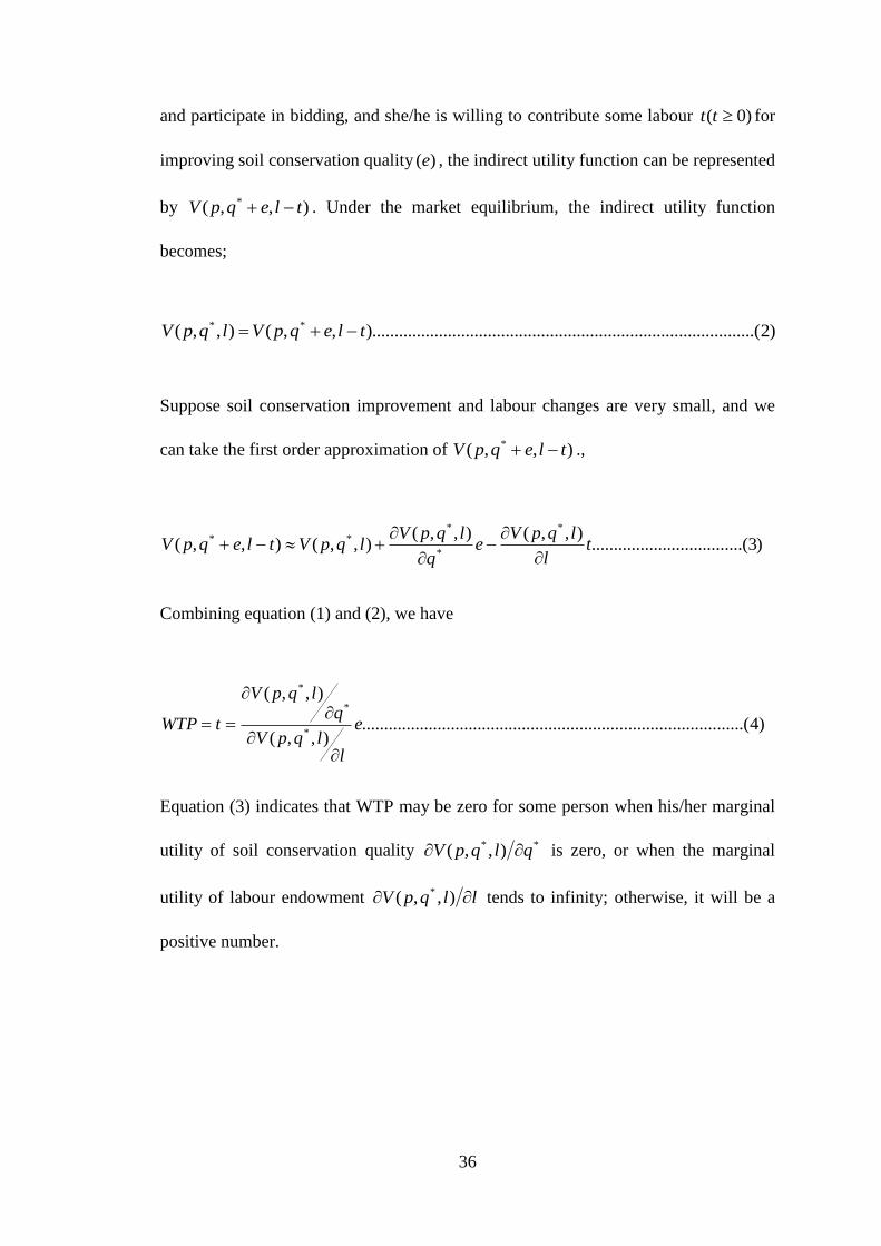
36
and participate in bidding, and she/he is willing to contribute some labour )0( tt for
improving soil conservation quality )(e , the indirect utility function can be represented
by ),,( * tleqpV . Under the market equilibrium, the indirect utility function
becomes;
)2.......(......................................................................).........,,(),,( ** tleqpVlqpV
Suppose soil conservation improvement and labour changes are very small, and we
can take the first order approximation of ),,( * tleqpV .,
)3....(..............................),,(),,(
),,(),,(*
*
*** t
l
lqpVe
q
lqpVlqpVtleqpV
Combining equation (1) and (2), we have
)4......(................................................................................),,(
),,(
*
*
*
e
llqpV
qlqpV
tWTP
Equation (3) indicates that WTP may be zero for some person when his/her marginal
utility of soil conservation quality ** ),,( qlqpV is zero, or when the marginal
utility of labour endowment llqpV ),,( * tends to infinity; otherwise, it will be a
positive number.

37
3.4.2 Empirical Model Specification
3.4.2.1 Estimation of Factors Affecting Willingness to Pay Model
The objective is to quantify the relationship between the individual characteristics and
the probability of household WTP for a randomly offered initial bid values. For a
given specified amount of labor that has to be subtracted from a given households‟
labor endowment for the proposed project soil conservation practices, farmers have
the choice either to accept the pre specified bid or not to accept for the dichotomous
choice question of the CVM survey. The decision process of the farmer can be
modeled in a simple utility framework following Hanemann (1984). Let the utility or
satisfaction of a given farmer is given by:
)5......(..........................................................................................).........,,( qZLUU ii
Where iU is the utility of the household i, L is total labour endowment of the
household in a year, Z are socio economic characteristics of the household, whereas q
is soil conservation quality as perceived by the farmer. Furthermore, let us assume
that there are two states of the world corresponding to different levels of soil
conservation quality: q* as the quality after the soil conservation practice is
undertaken and q as the quality before the soil conservation practices is undertaken or
if the practice is not pursued.
Since the total labour endowment of the particular household is a principal or most
limiting asset of the household, it is assumed that the individual will be willing to pay

38
the suggested reduction from its total labour endowment so as to maximize his or her
utility under the following condition or reject it otherwise;
)6.....(............................................................),,(),,( 0
0
1
*1eqZLUeqZBIDLU ii
Where iU , L, Z, q and q* are as defined above, BID is the initial labor payment
requirement per year for the soil conservation practices e1 and e0 are the error terms
which are with zero means and independently distributed. Therefore, the probability
that a household will decide to pay for the soil conservation is the probability that the
conditional indirect utility function for the proposed intervention is greater than the
conditional indirect utility function for the status quo.
It is worth mentioning that the utility functions are usually unobservable. The Utility
function of the ith
household which is assumed to be a function of observable
household characteristics; resource endowment and environmental quality, Xti, and a
disturbance term eti can be specified as;
)7.....(......................................................................,......2,11,0,)( niteXfU titi
t
i
The focus in this model is on the factors that determine the probability of accepting
the initial bid. The ith
farm household will be willing to accept the initial bid when
01
ii UU .Therefore, the choice problem can be modelled as binary response variable
Y, Where,
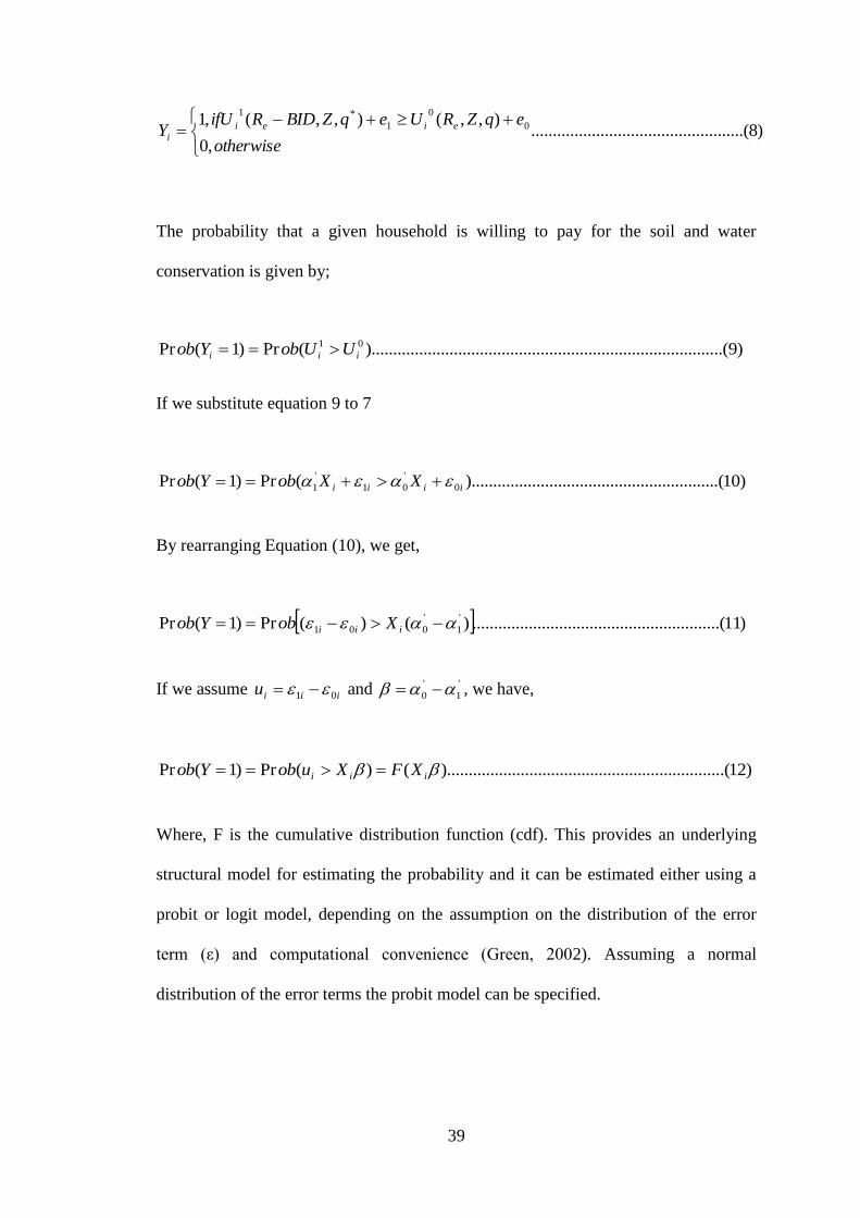
39
)8.........(........................................,0
),,(),,(,1 0
0
1
*1
otherwise
eqZRUeqZBIDRifUY eiei
i
The probability that a given household is willing to pay for the soil and water
conservation is given by;
)9..(......................................................................).........(Pr)1(Pr 01
iii UUobYob
If we substitute equation 9 to 7
)10........(........................................).........(Pr)1(Pr 0
'
01
'
1 iiii XXobYob
By rearranging Equation (10), we get,
)11.......(..................................................)()(Pr)1(Pr '
1
'
001 iii XobYob
If we assume iiiu 01 and '
1
'
0 , we have,
)12.....(..................................................).........()(Pr)1(Pr iii XFXuobYob
Where, F is the cumulative distribution function (cdf). This provides an underlying
structural model for estimating the probability and it can be estimated either using a
probit or logit model, depending on the assumption on the distribution of the error
term (ε) and computational convenience (Green, 2002). Assuming a normal
distribution of the error terms the probit model can be specified.

40
Following Hanemann (1984), the probit model can be specified as;
)13.(....................................................................................................'*
iii XY
Yi = 1 if Yi* ≥
t*
Yi= 0 if Yi* <
t*
Where:
'
= is vector of unknown parameters of the model
xi= is vector of explanatory variables
yi*= Unobservable households‟ actual WTP for soil conservation. y
i* is simply a
latent variable.
yi= Discrete response of the respondents for the WTP
*t i= the offered initial bids assigned arbitrarily to the i
th respondent
i = Unobservable random component distributed N (0, )
The respondents know their own maximum willingness to pay, yi*, but to the
researcher it is a random variable with a given cumulative distribution function (cdf)
denoted by F ( yi*; β) where β represents the parameters of this distribution, which
are to be estimated on the basis of the responses to the CVM survey.
3.4.3 Estimation of the Mean Willingness to Pay
The bivariate probit model was also used to estimate the mean WTP from the double
bounded dichotomous choice format. The mathematical estimation of the bivariate
probit model is presented below.

41
Let t1
be the first bid price and t2 be the second. The take-it-or-leave-it with follow up
format starts with an initial bid, t1. The level of the second bid depends on the
response to the first bid. That is, if the respondent answers „‟yes‟‟ for the initial bids,
she/he receives an upper follow-up bid t2; if she/he answers „‟no‟‟ for the initial bid, t
1
she/he receives a lower follow-up bid t2. In general, there are four possible outcomes:
both answers "yes"; both answers "no"; "yes" followed by a "no"; and "no" followed
by a "yes". The bounds on WTP are (Haab and McConnell, 2002):
1. 21 tWTPt for the yes-no responses;
2. 21 tWTPt for the no-yes responses;…………………….........................…..(14)
3. 2tWTP for the yes-yes responses;
4. 2tWTP for the no-no responses;
The most general econometric model for the double – bounded data comes from the
formulation below (ibid).
)15...(....................................................................................................jijij uWTP
Where ijWTP represents the ith respondent‟s willingness to pay, and j=1, 2 represents
the first and second answers. 1u and 2u are the means for the first and second
responses.
The probability of observing each of the possible two-bid response sequences (yes-
yes, yes-no, no-yes, no-no) can be represented as follows.

42
),Pr(),Pr(),Pr(
)16........().........,Pr(),Pr(),Pr(
),Pr(),Pr(),Pr(
),Pr(),Pr(),Pr(
2
22
1
11
2
2
1
1
2
22
1
11
2
2
1
1
2
22
1
11
2
2
1
1
2
22
1
11
2
2
1
1
tututWTPtWTPnono
tututWTPtWTPyesno
tututWTPtWTPyesyes
tututWTPtWTPnoyes
iiii
iiii
iiii
iiii
Each individual respondent (ith) contribution to the likelihood function becomes
)17...(....................),Pr(),Pr(
),Pr(),Pr()/(
2
22
1
11
2
22
1
11
2
22
1
11
2
22
1
11
NY
ii
NN
ii
YY
ii
YN
iii
tutuXtutuX
tutuXtututuL
Where YY=1 for a yes-yes answer, 0 otherwise, NY=1 for a no-yes answer, 0
otherwise, NN=1 for a no-no answer, 0 otherwise and YN=1 for a yes-no answer, 0
otherwise. Assuming the error terms are normally distributed with means 0 and
respective variances of σ12
and σ12, then WTP1i and WTP2i have a bivariate normal
distribution with mean u1 and u2, variances σ12
and σ12 and correlation coefficient ρ,
which is the covariance between the errors for the two WTP function.
Given the dichotomous choice responses to each question, the normally distributed
model is referred to as the bivariate probit model. The likelihood function for the
bivariate probit model can be derived as follows. The probability that WTP1i < t1 and
WTP2i < t2 i.e. the probability of a no-no response is;
)18.(..............................).........,,(),Pr(2
2
2
1
1
1
21
2
22
1
11
ututtutu ii
Where (.)21 is the standard bivariate normal cumulative distribution function with
zero mean, and unit variance and correlation coefficient ρ. Similarly the probability of
no- yes response is;
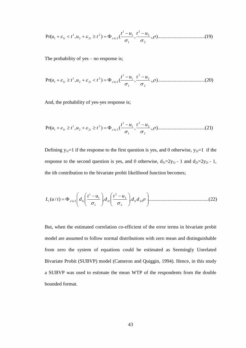
43
)19.........(....................).........,,(),Pr(2
2
2
1
1
1
21
2
22
1
11
ututtutu ii
The probability of yes – no response is;
)20.........(....................).........,,(),Pr(2
2
2
1
1
1
21
2
22
1
11
ututtutu ii
And, the probability of yes-yes response is;
)21.........(....................).........,,(),Pr(2
2
2
1
1
1
21
2
22
1
11
ututtutu ii
Defining y1i=1 if the response to the first question is yes, and 0 otherwise, y2i=1 if the
response to the second question is yes, and 0 otherwise, d1i=2y1i - 1 and d2i=2y2i - 1,
the ith contribution to the bivariate probit likelihood function becomes;
)22.........(........................................,,)/( 21
2
2
2
2
1
1
1
121
iiiii dd
utd
utdtuL
But, when the estimated correlation co-efficient of the error terms in bivariate probit
model are assumed to follow normal distributions with zero mean and distinguishable
from zero the system of equations could be estimated as Seemingly Unrelated
Bivariate Probit (SUBVP) model (Cameron and Quiggin, 1994). Hence, in this study
a SUBVP was used to estimate the mean WTP of the respondents from the double
bounded format.

44
Following, Green, (1997), a Bivariate Probit Model can be specified as:
2121
212211
212211
2
'
22
*
2
1
'
11
*
1
,|,
;1,|,|
)23...(............................................................;.........0,|,|
;
XXCov
XXVarXXVar
XXEXXE
Xy
Xy
Where: thiy *
1 respondent unobservable true WTP at the time of the first bid will
offered. WTP=1 if 1
*
1 Xy (initial bids), 0 otherwise.
thiy *
2 respondent implicit underlying point estimate at the time of the second bid is
offered.
The mean willingness to pay (MWTP) from bivariate probit model (Equation 16) can
be calculated using the formula specified by Haab and McConnell (2002).
MWTP …………………………..........................................……………….(24)
Where = a coefficient for the constant term
= a coefficient offered bids to the respondents

45
3.5 Definition of Variables
The Dependent Variable of the Model: The dependent variable is a binary choice
variable and measuring the willingness of households to pay for soil conservation
practices of labour contribution. The value of the dependent variable takes 1 for the
“yes” to the initial bid, zero otherwise.
The Independent Variables of the Model: With market imperfection, the
probability or the level of farm household‟s WTP for soil conservation depends on
various factors such as poverty and household characteristics, than only farm
characteristics (Tessema and Holden, 2006). Based on the findings of past studies on
households‟ willingness to pay for non market goods, decisions on investment and
participation, the following variables were hypothesized to determine household‟
willingness to participate in soil conservation practices.
Age of the house hold head (AGE): This is a continuous variable indicating the age
of the household head in years. The age of farm household head may have either
negative or positive effect on soil conservation willingness. Older age may shorten
planning time horizon and reduce the WTP; or it may relate to farm experience and
increase willingness to improve the soil for better productivity (Tessema and Holden,
2006). The longer farming experience, here equated with the older farmers is expected
to have a positive effect on conservation decision. On the other hand, young farmers
may have a longer planning horizon and, hence, may be more likely to invest in
conservation. Yitayal (2004), Tessema and Holden (2006), found a negative and
significant relationship, on the contrary, Demeke (2003), found a positive relationship

46
between age and soil conservation investment decisions. So, the effect of age of the
household head to willingness to pay for soil conservation can be positive or negative.
Education level of the Household head (EDUCATION): This is the number of
years that the household head had spent in a formal school. Household heads who
have high level of education can better understand the problem of soil erosion, hence
would be willing to contribute to the specified bid. Household heads with better
education are expected to understand consequences of degradation and be willing to
invest more in soil conservation (Tessema and Holden, 2006). Paulos (2002), reported
a positive relationship. It had a positive and strong relationship with the dependent
variable showing that literate household heads were more to recognize the advantages
of soil conservation and was willing to take part in it. Similarly, Yitayal (2004), in his
study in Jimma Zone found a positive relationship. So, the expected sign of Education
level of the household head is positive.
Social Position (SPOSITION): Is a dummy variable which takes 1 if the household
has some social position in its community; 0, otherwise. Social position of the
household head is expected to affect willingness to pay positively.
Household Size (FSIZE): It is a continuous variable which refers to the number of
family members of the household. This explanatory variable is included because it
affects the labour supply at household level. Some soil conservation technologies are
labour intensive and this may have a positive implication on whether the household
can decide to participate in the soil conservation practices.

47
Gender of the Household Head (SEX): This is recorded as dummy variable
(1=male, 0=otherwise) and is included in the model to find out the influence of
Gender for soil conservation willingness to pay. Male farmers have a probability of
getting more access to information than female household heads. Doss and Morries
(2001), as it is cited in Behailu (2009), confirmed that women farmers tend to adopt
improved technologies at a lower rate than men because of limited access to
information and resource. This can be further justified that soil conservation structures
need intensive labour so male headed households are expected to be more willing than
female headed households. It is, therefore, hypothesized that sex of the household
head will have a positive influence on the WTP.
Farm Size (FASIZE): It is a continuous variable expressed in terms of hectares of
cultivable land owned and expected to have a positive effect on the willingness of
farmers to pay for the soil conservation. This is because farmers who have more
cultivable land are expected to be more willing to devote some land for soil
conservation structure and are expected to pay for the soil conservation practices. This
hypothesis is similar to the findings of Paulos (2002), where total cultivable land was
found to be positively associated with willingness to pay for soil conservation.
Farmers’ perception of erosion hazard (PERCEPTION): This is a dummy which
takes 1 if the household perceives the problem of soil erosion, zero otherwise. The
recognition of the soil erosion problem is considered to be vital for soil conservation
decision. In other words, farmers who have already perceived the problem of soil
erosion are more likely to be willing to participate in soil conservation activities than
those who have not perceived the problem (Paulos, 2002). Thus, the perception

48
variable will be expected to be strongly and positively associated with farmers‟
willingness to pay for soil conservation.
Farm land forgone by erosion (FEROSION): This is a dummy variable which takes
1 if the farmer had abandoned a farm land because of soil erosion, zero otherwise. It is
expected to have a positive influence on willingness to pay.
Distance to the nearest market (DISTANCE): This is a continuous variable which
refers to the amount of time in minutes that a farmer spends to reach to the nearest
market from home. The average time the farmer must travel from the residential area
to the nearest market may have an effect on the willingness to pay for conservation
practices. It is hypothesized that the further away the residential area of the household
from the nearest market, less is expected to be willing to participate in soil
conservation practices because it is expected to compete with selling of products. So,
Distance to the nearest market is expected to have a negative effect on WTP.
Total livestock holding in Tropical Livestock Unit (TLU): This refers to the total
number of livestock (measured in Tropical Livestock Units, TLU) the farmer owns. In
Ethiopia, livestock are important source of cash income, food, household energy,
manure and source of power for cultivation. It is, therefore, hypothesised that the
higher the livestock holding the higher the household will be willing to pay for soil
conservation practices.
Farm Income (FARMINC): This is a continuous variable which is the total income
from crop production, animal selling, off farm income as well as remittance that the

49
household gets in a year, valued in Ethiopian birr. It is expected to have a positive
relationship with WTP.
Perception to Security of Tenure (TENURE): A dummy variable, which is a proxy
for security of land tenure that takes a value 1 if the peasant considered that he/ she
would be able to use the plot area at least during his/her life time, zero otherwise. The
incentive to land improvement decision is based on part of secured future access to
land. Hence, a positive effect was expected.
Frequency of extension contact (FREQEXTENSION): This is continuous variable
which is the number of days that the farmer had contact with extension agent in a
year. Extension is a way of building the human capital of farmers by exposing them to
information that reduces uncertainty (Feder et al. 1985). In this study this variable is
expected to affect willingness for soil conservation of farmers positively. This is
because extension intervention is expected to strengthen technology usage of the
farmers which further improves the income status and thus resulting in increase in the
willingness of the households to use soil conservation practices.
Labour Shortage (LSHORTAGE): This is a dummy variable which takes 1 if the
household has a labour shortage for farm activities and had hired some labour for
farm activities and 0, otherwise. We expect to have a negative relationship with
willingness to pay.
Amount of Credit: This is a continuous variable which is the amount of money that
the household gets in the past two year from formal and informal credit sources.

50
Credit might relax cash constraint and might enhance willingness to pay. Hence, it
was hypothesized that there would be a positive relationship.
Initial offered Bid (BID1): This is bid price offered to the respondents. In this study
the bid price was used as one of the explanatory variables in the analysis. The bid
price is expected to influences negatively to the willingness to pay of the
respondents‟.
The purpose of this chapter was to present the methodology that was used in the
study. A two stage simple random sampling was used to select the sampled
households for the final study. Data were collected through face to face interview via
trained enumerators. Descriptive statistics as well as econometric models were
developed to analyse the collected data from the sampled households. The variables
that were used in the econometric model were also defined in this chapter.
51
CHAPTER FOUR
4.0 RESULTS AND DISCUSSION
This chapter presents, the results obtained from the sample respondents. The first
section provides descriptive statistics of the survey results. The second section deals
with the analysis of determinants of respondents‟ WTP for soil conservation practices.
The last section computes mean WTP, estimation of total WTP and aggregate demand
for soil conservation practices. The descriptive analysis made use of tools such as
mean, percentages, standard deviation and frequency. Econometric analysis was used
to identify the determinants of willingness to pay and to estimate the parametric mean
of WTP. The statistical significance of the variables was tested using chi-square (χ2)
and F statistics.
4.1 Descriptive Statistics
4.1.1 Summary of Households’ Characteristics
For this study, data were collected from 225 randomly selected respondents. Data
from 218 respondents were utilized for the analysis. From the total sample of 218, 154
which are 70.6% of the respondents were male headed households and 64 which are
29.4% were female headed households. Out of the total sample households taken 128
(58.72%) were willing to take and contribute the pre specified initial offered bid and
90 (41.28%) of the households were not willing to pay the initially offered pre
specified bid. Out of all the 90 non willing households, male headed households
contribute 53.33 % while female headed households were 46.67%. On the other hand,

52
from the total 128 willing households, 82.81% were male headed households and
17.19% were female headed households. Table 4.1 indicates that there is strong
relationship between sex of the household head and willingness status to accept the
offered initial bid, which is significant at less than 1% probability level. This
underlines that, sex difference is an important component in WTP decision.
Table 4.1: Sex Composition of Sample Households
Non Willing Willing Total
SEX No. Percentage No. Percentage No. Percentage χ2
Male 48 53.33 106 82.81 154 70.6 22.14***
Female 42 46.67 22 17.19 64 29.4
Total 90 100 128 100 218 100
*** Significant at less than 1% Non-Willing is a “No” answer for the first bid while Willing is a “Yes” answer for the first bid
Source: Own Survey, 2012
In addition, out of the 154 male headed households, 48 (31.17%) of them were not
willing and the remaining 106 (68.83%) of them were willing to contribute the pre
specified initial bid offered amount of labor for soil conservation practices. From the
total 64 female headed households 42 (65.62%) were not willing to take the initial
person days offered and the remaining 22 (34.38%) were willing to take up the initial
bid of person days per year.
Table 4.2 shows the relationship of willingness to pay and marital status and social
position of households in the study area. Of the total farmers surveyed, 149 (68.35%)
were married, 69 (31.65%) were single (Divorced and Widowed). In addition, out of the
149 married respondents, 116 (77.6%) were willing and 33 (22.1%) were not willing.
Furthermore, 59.4 percent of the single respondents were not willing and the rest 40.6
percent were willing to pay the initial bid. In addition, there is also statistically

53
significant relationship between willingness status and marital status of the household
head showing that, marital status systematically and significantly relates with WTP
status. This is mostly because married households have the capacity to accept the
offered initial bid because they have more labour force (family size) than single
households.
Table 4.2: Household Characteristics Marital Status and Social Position
Non Willing Willing Total
Marital
status
No. Percentage No. Percentage No. Percentage χ2
Married 45 50 104 81.25 149 68.35 23.85***
Single 45 50 24 18.75 69 31.65
Total 90 100 128 100 218 100
Social Position
Yes 5 5.66 24 18.75 29 13.3 7.98**
No 85 94.44 104 81.25 189 86.7
Total 90 100 128 218 100 *** and ** significance level at less than 1% and 5% respectively
Source: Owen Survey, 2012
The sampled households had a total of 1320 family members averaging at about 6.06
with a minimum of 1 size and a maximum of 11 members in a household. The mean
household sizes of the willing and non willing households were 6.89 and 4.43,
respectively, and this difference is statistically significant at less than 1% probability
level; showing that there was a significance difference between the willing and non-
willing households in family size. This is because soil conservation practices are
labour intensive activities and family size is an important resource endowment (Table
4.3).
The mean of the number of years that the household head spent on school was also
computed as it is shown in Table 4.3. The result shows that, the mean of years that the
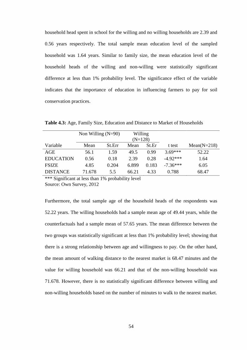
54
household head spent in school for the willing and no willing households are 2.39 and
0.56 years respectively. The total sample mean education level of the sampled
household was 1.64 years. Similar to family size, the mean education level of the
household heads of the willing and non-willing were statistically significant
difference at less than 1% probability level. The significance effect of the variable
indicates that the importance of education in influencing farmers to pay for soil
conservation practices.
Table 4.3: Age, Family Size, Education and Distance to Market of Households
Non Willing (N=90) Willing
(N=128)
Variable Mean St.Err Mean St.Er t test Mean(N=218)
AGE 56.1 1.59 49.5 0.99 3.69*** 52.22
EDUCATION 0.56 0.18 2.39 0.28 -4.92*** 1.64
FSIZE 4.85 0.204 6.899 0.183 -7.36*** 6.05
DISTANCE 71.678 5.5 66.21 4.33 0.788 68.47
*** Significant at less than 1% probability level
Source: Own Survey, 2012
Furthermore, the total sample age of the household heads of the respondents was
52.22 years. The willing households had a sample mean age of 49.44 years, while the
counterfactuals had a sample mean of 57.65 years. The mean difference between the
two groups was statistically significant at less than 1% probability level; showing that
there is a strong relationship between age and willingness to pay. On the other hand,
the mean amount of walking distance to the nearest market is 68.47 minutes and the
value for willing household was 66.21 and that of the non-willing household was
71.678. However, there is no statistically significant difference between willing and
non-willing households based on the number of minutes to walk to the nearest market.

55
4.1.2 Resources Ownership
The survey results showed that the households possession of cultivable land ranged
from the smallest 0.125 ha (which is equivalent to half a „‟timad‟‟) to the highest 2.5
ha (which is equivalent to 5 „‟timad‟‟). The average size of cultivated land owned by
the sample respondents was about 0.61 ha. Willing farmers owned on the average
0.66 ha of cultivated land. The corresponding figure for the non-willing farmers was
0.504 ha. The mean difference of own cultivated land for the two groups was
significant at 5 % significance level (Table 4.4). This means, willingness tends to
increase as farm size increases. This is probably because soil conservation practices
take proportionally more space on small land holdings and the benefit from such
practices on these small land holdings will not be enough to compensate for the
decline in production due to the loss in area devoted to the conservation structures. On
the other hand, households who have small land holdings may need to subsidize their
income from off farm activities given productions are low from small land holdings
and might not get time to spend on conservation practices.
Table 4.4: Farm Size, Income and TLU Ownership of Sampled Households
Non Willingness
(N=90)
Willing N(128)
Variable Mean St.Err Mean St.Er t test Mean(N=218)
FASIZE 0.54 0.026 0.652 0.032 -2.57** 0.605
INCOME 4781.29 354.06 7865.98 316.4 -6.42*** 6592.48
TLU 2.95 0.22 5.45 0.222 -7.81*** 4.42
FASIZE= Total farm Size INCOME= Total income TLU= Total Livestock Units
*** and ** statistically significant at 1% and 5% respectively
Source: Own Survey, 2012
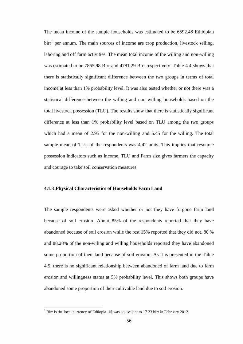
56
The mean income of the sample households was estimated to be 6592.48 Ethiopian
birr1 per annum. The main sources of income are crop production, livestock selling,
laboring and off farm activities. The mean total income of the willing and non-willing
was estimated to be 7865.98 Birr and 4781.29 Birr respectively. Table 4.4 shows that
there is statistically significant difference between the two groups in terms of total
income at less than 1% probability level. It was also tested whether or not there was a
statistical difference between the willing and non willing households based on the
total livestock possession (TLU). The results show that there is statistically significant
difference at less than 1% probability level based on TLU among the two groups
which had a mean of 2.95 for the non-willing and 5.45 for the willing. The total
sample mean of TLU of the respondents was 4.42 units. This implies that resource
possession indicators such as Income, TLU and Farm size gives farmers the capacity
and courage to take soil conservation measures.
4.1.3 Physical Characteristics of Households Farm Land
The sample respondents were asked whether or not they have forgone farm land
because of soil erosion. About 85% of the respondents reported that they have
abandoned because of soil erosion while the rest 15% reported that they did not. 80 %
and 88.28% of the non-wiling and willing households reported they have abandoned
some proportion of their land because of soil erosion. As it is presented in the Table
4.5, there is no significant relationship between abandoned of farm land due to farm
erosion and willingness status at 5% probability level. This shows both groups have
abandoned some proportion of their cultivable land due to soil erosion.
1 Birr is the local currency of Ethiopia. 1$ was equivalent to 17.23 birr in February 2012

57
Based on farmers understanding of slope and possibility of plots for oxen plough and
hoe cultivation, farm plots were classified into four. These were; relatively flat farm
plots, gently sloped farm plots, plots that have very steep slope but possible for oxen
plough and plots that is very steep slope not possible for oxen plough. Out of the total
sample surveyed, 2.29 % households had very steep slope lands (Table 4.5) and 50 %
of the households had lands which are steep sloped, 41.28 % of the farmers have
gently sloped lands. Only 6.43 % of the farmers had relatively flat plots. This shows
how soil erosion is a serious problem in the study area. But, the results in Table 4.5
show that there is no statistically significant relationship.
Table 4.5: Physical Characteristics of Households Farm Land
Non Willing Willing Total
No. Percentage No. Percentage No. Percentage χ2
Farm Erosion
Yes 72 80 113 88.28 185 84.86 2.82
No 18 20 15 11.72 33 15.14
Total 90 100 128 100 218 100
Farm Land Exposure to Erosion
No risk 9 10 7 5.47 16 7.34
2.62 Medium 63 70 101 78.91 164 75.23
High
Exposure 18 20 20 15.62 38 17.43
Total 90 100 128 100 218 100
Average Slope of Farm Land
Very Steep 2 2.22 3 2.34 5 2.29
5.14 Steep 48 53.33 61 47.66 109 50
Gentle slope 31 34.45 59 46.1 90 41.28
Flat 9 10 5 3.9 14 6.43
Total 90 100 128 100 218 100
Source: Own Survey, 2012
58
4.1.4 Perception of Soil Erosion Hazard
The level of perception of soil erosion problem is positively associated with age of the
household head, the level of education of the household head and diffusion of
information through extension and other channels (Shiferaw and Holden, 1998).
Generally speaking, perception of soil erosion problem is an important factor for
farmers to make decisions on conservation investments (Paulos, 2002). In the country
(Ethiopia) in general, and in the study site in particular, soil erosion is accelerated by
an alarming rate mainly because of expansion of farmland to hillsides by clearing the
natural vegetation. In spite of this fact the extension advice provided to farmers
regarding soil conservation and the practical actions being taken are minimal as
compared to the severity of the problem (Paulos, 2002).
Table 4.6: Perception of Soil Erosion Hazard
Non Willing Willing Total
No Percentage No Percentage No Percentage χ2
Perception
Yes 85 94.44 127 99.22 212 97.25 4.5**
No 5 5.66 1 0.78 6 2.75
Total 90 100 128 100 218 100
Source: Own Survey, 2012 ** Significance at 5%
More than 99% of the respondents who were willing to take the pre specified initial
bid in soil conservation practices perceived soil erosion as a problem in their area.
Similarly more than 94% of the non-willing households also perceive the problem of
soil erosion in their area. This shows that the problem of soil erosion hazard is well
perceived in the study area and there is a need to take action. Table 4.6 shows that
there is statistically significant relationship between willingness status and perception

59
of soil erosion hazard at less than 5% probability level showing that perception of soil
erosion hazard increases willingness to pay.
4.1.5 Land Tenure
Land tenure system which is the result of a complex interrelated linkage of social,
cultural, economical, political and institutional system needs a special attention. In
Ethiopia, government owns land and farmers have uses right and they can also rent
their land (Behailu, 2009). The sampled households were also classified based on
tenure security of their farm lands. 98.43 percent of the respondents who were willing
to take the offered initial bid for soil conservation practices were secured that their
farm land will be with them at least until their life time. Of the 90 respondents who
were not willing to participate in soil conservation practices, 78.89% were secured
that their farm land will be with them at least until their life time (Table 4.7). Table
4.7 shows that there is a statistically significant relationship between land tenure
security and willingness to pay at less than 1% probability level showing that land
tenure security is an important variable for households decision to participate in soil
conservation practices. This implies that security of land at least until life time gives
farmers opportunity to invest in soil conservation practices.
Table 4.7: Land Tenure Security of Sampled Households
Non Willing Willing Total
No Percentage No Percentage No Percentage χ2
Land Tenure
Yes 71 78.89 126 98.43 197 90.37 23.2***
No 19 21.11 2 1.57 21 9.63
Total 90 100 128 100 218 100
Source: Own Survey, 2012 *** significant at 1% probability level

60
4.1.6 Labor Availability
Any form of soil conservation activity demands labor input. In order to undertake the
practice, farm households need to take some labor away from their farm activities
(Paulos, 2002). Table 4.8 shows that a large number of non-willing farmers (about
38.89%) reported labor shortage as a problem as compared to the willing household
which was only 13.28 percent. As can be seen in the Table 4.8, 23.85% of the total
respondents had reported labor shortage as a problem, whereas labor shortage was not
reported as a problem by 76.15% of the respondents and there was a statistically
significant relationship between willingness status and problem of labor shortage.
Showing that, labor is an important factor in determining willingness to pay for soil
conservation practices.
Table 4.8: Labor Availability of Households
Non Willing Willing Total
No Percentage No Percentage Number Percentage χ2
Labour Shortage
Yes 35 38.89 17 13.28 52 23.85 19.08***
No 55 61.11 111 86.72 166 76.15
Total 90 100 128 100 218 100
Source: Own Survey, 2012 *** statistically significant at 1% probability level
4.2 Analysis of Determinants of Households’ WTP
Estimation results of the probit model are reported based on the theoretical model that
has already been developed in chapter three. The model was used to examine whether
WTP for soil conservation of surveyed households are related to the explanatory
variables or not. A total of 16 explanatory variables were considered in the
61
econometric model out of which only 8 variables were found to significantly
influence the probability of willingness to pay among the farm households at less than
5% probability level.
Before running the econometric model, the independent (continuous) variables were
tested for the presence of multicollinearity (Appendix IV). The result showed that
there were no multicollinearity problems between the variables. The value for
Contingency Coefficient(CC) (Appendix V) for the dummy variables were less than
0.75 and the value of Variance Inflation Factor (VIF) for the continuous variables
were less than 10; which are obviously the indicators for the absence of
multicollinearity.
The chi-square (χ2) distribution is used as the measure of overall significance of a
model in probit model estimation. The result of the probit model shows that, the
probability of the chi-square distributions (192.9) with 16 degree of freedom less than
the tabulated counterfactual is 0.0000, which is less than 1%. So, this shows that, the
variables included explaining willingness to pay fits the probit model at less than 1%
probability level. This implies that the joint null hypothesis of coefficients of all
explanatory variables included in the model were zero should be rejected. In general,
it shows that, the data fits the model very well. The results are given in Table 4.9.
As indicated in Table 4.9 of the probit estimate, out of the total 16 explanatory
variables hypothesized, 6 explanatory variables have positive and significant effects
on probably of respondents accepting the offered initial bid, and 2 had negative and
significant effect to the log likelihood of the probit model. On the other hand the rest
8 explanatory variables were found to be not significant at 5% probability level.

62
Table 4.9: Probit Model Estimates of WTP
Variables Coefficients Stad. Err Z-Value P-Value
AGE -0.0396*** -0.0129 -3.07 0.0020
SEX 0.712** -0.3480 2.05 0.0410
EDUCATION 0.309*** -0.0956 3.23 0.0010
SPOSITION 1.730 -0.9230 1.88 0.0610
DISTANCE 0.000704 -0.0032 0.22 0.8260
FSIZE 0.238** -0.0941 2.53 0.0110
FASIZE 0.384 -0.6370 0.6 0.5470
PERCEPTION 4.674*** -1.5710 2.97 0.0030
FEROSION -0.365 -0.4840 -0.75 0.4510
BID1 -0.0458*** -0.0100 -4.58 0.0000
LSHORTAGE -0.681 -0.4110 -1.66 0.0980
EXTFREQUENCY 0.0113 -0.0227 0.5 0.6200
TENURE 2.074** -0.8220 2.52 0.0120
INCOME 7.87E-05 -0.0001 1.37 0.1690
TLU 0.245*** -0.0910 2.69 0.0070
AMCREDIT -5.98E-05 -0.0001 -1.1 0.2710
CONSTANT -5.784*** -2.0230 -2.86 0.0040
Observations 218
Log likelihood -48.37
LR chi2 (16) 192.9
Pseudo R2 0.666
Prob>Chi2 0.0000
*** &** Significance at 1% and 5% respectively
Source: Own Survey, 2012
In the determinants of willingness to pay estimation of the probit model, the not
significant explanatory variables were less important in explaining the variability in
the willingness to pay. Thus, in this study only the significant explanatory variables
were discussed below. However, it is noticed that, the non significant variables have
also contributed to the log likelihood function of the probit model.
Age of the household head (AGE): Age of the household head had negative effect
on the willingness to pay of households for soil conservation practices. It had negative
and significant effect on households‟ WTP in person day‟s contribution at less than

63
1% level of significant. The descriptive statistics also shows there is a significant
difference between the two mean.
The negative and significant correlation between age and willingness to pay for soil
conservation practices might be perhaps because of two reasons. Older age may
shorten planning time horizon and reduce the WTP. Thus, older are less likely willing
to pay for soil conservation practices as they expect they would benefit less from the
investment relative to young household heads, given that the benefits are generally
longer term in nature. On the other hand, young farmers may have a longer planning
horizon and, hence, may be more likely to be willing for conservation. Besides, an
older aged household heads are more likely to have a labour shortage and reduce
willingness to pay for soil conservation practices. The negative relationship between
age and investment for environmental protection is consistent with the findings of
Tegegne (1999), Yitayal (2004), and Solomon (2004).
Sex of the household head (SEX): Unlike age of the households, sex of the
household head was found to have a positive effect to willingness to pay for soil
conservation. The result of probit model revealed that male headed household heads
were found to be willing to pay more for soil conservation practices than female
headed households. The sign of sex turned out to be consistent with the prior
expectation and it was positively and significantly related with the dependent variable
at less than 5% level of significance. Alemu (2000), and Animut (2006), reported the
same result. This is mainly because; female headed households have less resources
possession endowment as well as some cultural constraints than meal headed
households.

64
Education level of the household head (EDUCATION): This variable took the
expected sign and its coefficient was significant at less than 1 percent probability
level. It had a positive and strong relationship with the dependent variable showing
that as the education level of the household head increases, willingness to pay for
conservation practices increases. This could be possibly because, education increases
environmental awareness and value for environmental goods such as soil. Tegegne
(1999), and Paulos (2002), reported a similar result.
Family size of the household (FSIZE): The coefficient of this variable supports the
proposed hypothesis and it was found to be significant at 5 percent probability level.
Households with higher family size are expected to pay more than those who have
less family size because the proposed project was by labour contribution. This is
precisely because soil conservation practices are labor intensive to build and maintain,
hence households with large labor may tend to pay more for conservation. The
implication of the positive sign is that an increase in household family size increases
the probability of a respondent to support the proposed voluntary labour contributions
to soil conservation.
Perception of soil erosion (PERCEPTION): The sign of perception of soil erosion in a
plot is turned out to be consistent with the a priori expectation and it was positively and
strongly related with the yes answer to the first initial bid offered. That is, households that
have perceived the problem of soil erosion in the study are willing to pay more than
the farmers who didn‟t perceive the problem of soil erosion in their plot land. The
coefficient of this variable was significant at 1% probability level. Paulos, (2002) also
found similar result.

65
Initial bid offered (BID1): Initial bid offered has been found to be negative and
significantly related at 1% significance level with willingness to pay for conservation
practices. This implies, the probability of a yes response to the initial bid increases
with decrease in the offered initial bid which indicates that the likelihood of accepting
an offered bid amount increases as the bid amount goes down and vice versa which is
consistent with the economic theory.
Land Tenure (TENURE): The coefficient of the variable land tenure appeared to be
significant at 5% probability level with the expected sign. The implication of the
positive sign is that a perception of security of the cultivated land at least until life
time increases the probability of a farmer to support the proposed voluntary labour
contributions. This result implies that it is land tenure security of farm land is an
important determinant of the WTP for soil conservation practices.
Total Livestock Unit (TLU): TLU has an expected positive effect related to
likelihood of saying yes to the first bid. The coefficient of this variable was significant
at 1% probability level which shows TLU possession increases WTP. Livestock is
considered as a measure of wealth and increased availability of capital which make
WTP in soil conservation more feasible. The empirical findings by Jonse (2005),
indicated that number of livestock in terms of tropical livestock unit plays an
important role for willingness to pay. This is consistent with the fact that TLU is one
of the wealth indicators and should have a positive contribution to willingness to pay.
In general, in the probit model farm land forgone because of erosion (FEROSION),
distance to the nearest market (DISTANCE) and amount of credit received within the
past two years (AMCREDIT) has the unexpected signs but statistically insignificant

66
with the prior expectations. Other variables such as total farm size (FASIZE), social
position of the household head (SPOSITION), Labour shortage for farm activities
(LSHORTAGE), frequency of extension visit in a year (EXTFREQUENCY) and total
income (INCOME) has expected sign but statistically not significant at 5%.
It is clear, however, that the coefficients of the probit model do not indicate the
marginal effects of explanatory variables on the variation of the dependent variable.
That is, in the probit model only the signs (not the magnitudes) of the coefficients of
independent variables are important. In order to analyze the effects of each
explanatory variable on the probability that the respondent accepts the initial offered
bid or rejects it, the partial derivatives of the dependent variable with respect to each
explanatory variable must be taken (Greene, 1993). The marginal effects of the probit
model estimation results are reported in the Table 4.10 below.
The interpretation of the marginal effects of the probit model indicates the change in
the likelihood occurrence of an event due to the change of dummy variables from 0 to
1 and a unit change from the mean in the continuous explanatory variables at a time
keeping the other variables constant at their mean.
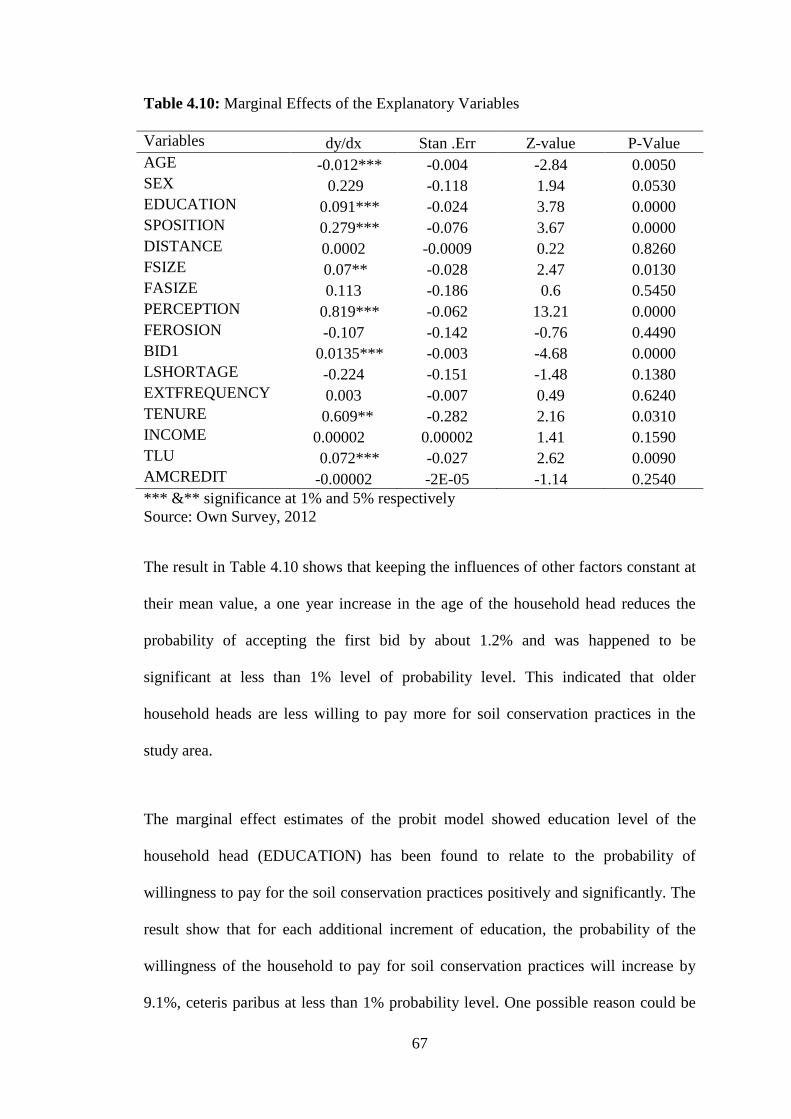
67
Table 4.10: Marginal Effects of the Explanatory Variables
Variables dy/dx Stan .Err Z-value P-Value
AGE -0.012*** -0.004 -2.84 0.0050
SEX 0.229 -0.118 1.94 0.0530
EDUCATION 0.091*** -0.024 3.78 0.0000
SPOSITION 0.279*** -0.076 3.67 0.0000
DISTANCE 0.0002 -0.0009 0.22 0.8260
FSIZE 0.07** -0.028 2.47 0.0130
FASIZE 0.113 -0.186 0.6 0.5450
PERCEPTION 0.819*** -0.062 13.21 0.0000
FEROSION -0.107 -0.142 -0.76 0.4490
BID1 0.0135*** -0.003 -4.68 0.0000
LSHORTAGE -0.224 -0.151 -1.48 0.1380
EXTFREQUENCY 0.003 -0.007 0.49 0.6240
TENURE 0.609** -0.282 2.16 0.0310
INCOME 0.00002 0.00002 1.41 0.1590
TLU 0.072*** -0.027 2.62 0.0090
AMCREDIT -0.00002 -2E-05 -1.14 0.2540
*** &** significance at 1% and 5% respectively
Source: Own Survey, 2012
The result in Table 4.10 shows that keeping the influences of other factors constant at
their mean value, a one year increase in the age of the household head reduces the
probability of accepting the first bid by about 1.2% and was happened to be
significant at less than 1% level of probability level. This indicated that older
household heads are less willing to pay more for soil conservation practices in the
study area.
The marginal effect estimates of the probit model showed education level of the
household head (EDUCATION) has been found to relate to the probability of
willingness to pay for the soil conservation practices positively and significantly. The
result show that for each additional increment of education, the probability of the
willingness of the household to pay for soil conservation practices will increase by
9.1%, ceteris paribus at less than 1% probability level. One possible reason could be
68
that more educated individuals are concerned about environmental goods including
soil in our case.
In addition, the result of the probit model showed that having social position in the
study area was positively and significantly related to the probability of yes for the
offered initial bid for conservation practices at less than 1 % probability level. This
implies that farmers who have some social position in the study area are more willing
to pay for the conservation practices. The reason might be due to the fact that having
some social position increases responsibility hence willingness to pay for soil
conservation practices. The estimated coefficient of 0.279 indicates having some
social position increases willingness to pay by 27.9 percent.
The estimated coefficient of the total family size (FSIZE), which is one of the most
crucial explanatory variables of probability of WTP, was found to be statistically
significant at the 5% level with the expected positive sign. This indicates that the
probability of WTP to support the proposed soil conservation practices increases as
the total household size increases under the hypothetical market scenario. Keeping the
influence of other factors constant, a 1 person increase in the total family size
increases the probability of willingness to pay by 7%. This is precisely because soil
conservation practices are labor intensive to build and maintain, hence households
with large labor are willing to invest more in conservation.
Perception about the existence of problem of soil erosion was happened to take the
expected sign and significant at less than 1% probability level. Holding other things
constant, the probability of a household willingness for conservation increases by
69
81.9% for perceived farmers than the other counter factual. This implies that,
perception of soil erosion problem plays an important role in WTP decision.
Consistent with the earlier expectation and economic theory, the initial bid offered
(BID1) has a negative and significant effect on the WTP for soil and water
conservation practices at less than 1% level of significance. The marginal effect
indicates that a one person days increase for the contribution of the proposed project
reduces the probability of being willing to pay by nearly 1.4%.
The security of land at least until lifetime (TENURE) was positively and significantly
related to the households‟ WTP to support the proposed conservation practices. This
variable was expected and significant at less than 5% probability level. Holding other
variables at their respected mean, a perception of land security at least until life time
increases the household‟s WTP to support conservation practices by approximately
60.9 percent. This result implies that it is not only the capability of the farmers but
also their perception of land security that influences the decision to participate in soil
conservation practices.
Total Livestock Unit (TLU) has been found to relate to the probability of willingness
to pay for soil conservation practices positively and significantly. TLU could be a
proxy for wealth under Ethiopian farmers‟ condition. When the wealth of a household
increases, the willingness to pay will also increase. The marginal effect show that for
each additional increment of TLU, the probability of the willingness of the household
to pay for the conservation practices will increase by 7.2%, keeping the other
explanatory variables at their mean. This is consistent with the fact that TLU is one of
the wealth indicators and should have a positive contribution to willingness to pay.

70
4.3 Households Willingness to Pay for Soil Conservation Practices
4.3.1 Descriptive Statistics of the Discrete Responses
The bid sets were randomly distributed to the questionnaire. These initial and second
bids were obtained during the pilot survey and focus group discussion. For each initial
bid offered (bid1), there are two possible responses. The first row for each initial bid
summarizes the “no” response to that bid. The second row for each bid summarizes
the “yes” responses. An initial bid of 22 person days per year resulted in 57 “yes”
responses and 16 “no” responses. Of the 57 “yes” responses to BID1=22, the follow
up bid (BID2=44) resulted in 41 “yes” and 16 “no” responses and out of the 16 “no”
responses for the initial bid (BID1=22) the follow up bid (BID2=11) resulted in 5 and
11 “yes” and “no” responses respectively. Similarly, the second initial bid (BID1=40)
man days per year resulted in 46 “yes” and 26 “no” responses. The follow up bid for
the 46 “yes” responses of the second initial bid (BID1=40), which is BID2=80,
resulted in 29 “yes” and 17 “no” responses, while the “no” responses to the second
initial bid, which is BID2=20, resulted in 12 “yes” and 14 “no” responses. Finally, the
third initial bid (BID1=65) was resulted in 25 “yes” and 48 “no” responses. The 25
“yes” responses of the third initial bid have produced 9 “yes” and 16 “no” responses
for the amount of bid offered in the second question, which was 130 person days per
year. On the other hand, the 48 “no” responses for the third initial bid have produced
24 each “yes” and “no” answers for the bid offered in the second question, which was
32 person days per year. In general, a total of 436 responses were obtained for the
analysis from the double bounded dichotomous question.

71
Table 4.11: Summary of Discrete Responses to the Double- Bounded Questions
First Question Second Question
Initial Price
(BID1)
Follow
Up Price
(BID2)
No. of „yes‟
responses to
the initial
price
No. of „No‟
responses to
the initial
price
No. of „yes‟
responses to
the Follow up
price
No. of
„No‟
responses
to the
Follow up
price
22 11 0 16 5 11
22 44 57 0 41 16
40 20 0 26 12 14
40 80 46 0 29 17
65 32 0 48 24 24
65 130 25 0 9 16
Source: Own Survey, 2012
Households were also categorized based on their joint responses to the offered bids
(initial and follow up). The results revealed that about 22.5% of the households
rejected the initial offers as well as the follow up discounted bids (no-no). Of the 218
surveyed respondents, the percentage of households that did not accept the initial bid
but accepted the second discounted bid was found to be 19%. The third category of
households presented in Table 4.10 was those households that accepted the initial bid
but rejected the higher second follow up bid. This category accounts 22.5% of the
households. The fourth category represents households who had yes-yes responses for
the first initial bid as well as for the higher follow up bids. Those households were
36% of the total sampled households.
The frequency Table 4.12 of the willingness to pay category showed that the highest
frequency was observed in the fourth willingness to pay category of households in
which, the households accepted the offered initial bids as well as the second higher
bids. This was followed by the “no-no” and “yes-no” categories which constitutes
22.5% each of the sampled households. Finally, the 2nd
category of households in

72
which their responses were “no” to the initial bids followed by “yes” to the follow up
lower second bids placed on the 4th
rank with a percentage of 16.
Table 4.12: Frequency of Willingness to pay
WTP Category Frequency Percent
No –No 49 22.5
No –Yes 41 19
Yes –No 49 22.5
Yes- Yes 79 36
Total 218 100
Source: Own Survey, 2012
4.2.2 Estimation of Mean from Double Bounded Dichotomous Choice Format
Table 4.13 presents the descriptive statistics of households‟ responses to the offered
bids in the double bounded dichotomous choice format. The result shows that the
average initial bid was 42.34 person days per year. Whereas, the average second bid
for soil and water conservation practices was 54.63 person days per year. The “yes”
response for the first bid offered is about 59% while the “yes” responses for the
second bid were about 55%.
Table 4.13: Descriptive Statistics of the Dichotomous Choice Format
Variable Observation Mean Stan. Dev Min Max
BID1 218 42.34404 17.7124 22 65
BID2 218 54.63303 34.7513 11 130
VBID1 218 0.587156 0.4934784 0 1
VBID2 218 0.5504587 0.4985923 0 1
Source: Own Survey, 2012
As it is discussed in the methodology part, the main objective of the double bounded
dichotomous choice format was to estimate the mean WTP from responses of both the
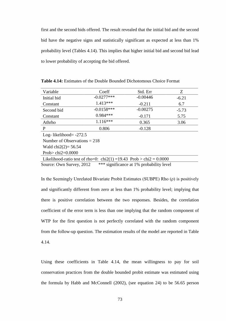
73
first and the second bids offered. The result revealed that the initial bid and the second
bid have the negative signs and statistically significant as expected at less than 1%
probability level (Tables 4.14). This implies that higher initial bid and second bid lead
to lower probability of accepting the bid offered.
Table 4.14: Estimates of the Double Bounded Dichotomous Choice Format
Variable Coeff Std. Err Z
Initial bid -0.0277*** -0.00446 -6.21
Constant 1.413*** -0.211 6.7
Second bid -0.0158*** -0.00275 -5.73
Constant 0.984*** -0.171 5.75
Athrho 1.116*** 0.365 3.06
Ρ 0.806 -0.128
Log- likelihood= -272.5
Number of Observations = 218
Wald chi2(2)= 56.54
Prob> chi2=0.0000
Likelihood-ratio test of rho=0: chi2(1) =19.43 Prob > chi2 = 0.0000
Source: Own Survey, 2012 *** significance at 1% probability level
In the Seemingly Unrelated Bivariate Probit Estimates (SUBPE) Rho (ρ) is positively
and significantly different from zero at less than 1% probability level; implying that
there is positive correlation between the two responses. Besides, the correlation
coefficient of the error term is less than one implying that the random component of
WTP for the first question is not perfectly correlated with the random component
from the follow-up question. The estimation results of the model are reported in Table
4.14.
Using these coefficients in Table 4.14, the mean willingness to pay for soil
conservation practices from the double bounded probit estimate was estimated using
the formula by Habb and McConnell (2002), (see equation 24) to be 56.65 person

74
days per year per household for five years. At 95% confidence interval the WTP
varies between 51.01 to 62.29 person days per year. The result shows that the mean
WTP from double bound format was greater than the mean value from the open ended
response which was computed at 48.94 person days per year per household for five
years.
4.3.1 Analysis of Results of the Open Ended Format
In the open ended question, respondents were asked to state the maximum amount
they would like to pay for soil conservation practices. The amount of labour that the
households would contribute to the proposed project ranges from 0 to 152 person days
per year for five years. Table 4.15 presents the frequency distribution of farm
households‟ WTP in person days per year for five years. The table shows that about
83.49 % of the farmers were willing to pay some amount of labor for soil
conservation practices. In the practice of CVM, 0 bidders are presented with follow-
up questions to ascertain whether they are expressing a protest bid against the
valuation or they place no value on the resource (Paulos, 2002).
Table 4.15: Willingness to Pay of Households Based on the Open Ended Format
Willingness to pay of households
(Open Ended Question)
Frequency Percent
Non Willing (0) 36 16.51
Willing(>0) 182 83.49
Total 218 100
Source: Owen survey, 2012
The frequency distribution of the responses of the sampled households of the open
ended responses is also presented in the Table 4.16.

75
Table 4.16: Frequency Distribution of the Open Ended Questionnaire Format
Number of person days Number of farmers Percent
0 36 17
10-25 33 15
26 – 41 33 15
42 – 57 30 14
58 – 73 31 14
74 – 89 26 12
90 – 105 20 9
106 – 121 1 0
122 – 137 4 2
138 – 153 4 2
Observations 218
Mean 48.94
Standard Deviation 35.72
Maximum 150
Minimum 0
Source: Owen survey, 2012
Table 4.16 shows distribution of farmers‟ willingness to spend person days on soil
conservation practices in a year. Of the 218 sample respondents 36 were not willing to
contribute any labor for soil conservation practices. On the other hand, the remaining
182 were willing to contribute some amount of labor. The average number of days
that farmers were willing to contribute for soil conservation practices was 48.94.
Figure 4.1 shows the frequency curve of sample households‟ maximum willingness to
contribute labor for soil conservation practices in a year. The curve shows that lower
numbers of respondents recoded in the higher bids.

76
Figure 4.1: Ferequency Curve for Soil Conservation
Source: Own survey, 2012
4.3.2 Reasons for Maximum Willingness to pay
Respondents were asked to point out their major reasons for their maximum
willingness to pay. Of the 218 sampled households included in the analysis 83.49% of
the households state their reason for maximum willingness to pay. The rest 16.51% of
the sampled households were missing because they were not willing to pay any
amount of person days for the proposed project of soil conservation practices.
Table 4.17: Reasons for Maximum Willingness to Pay
Reason For maximum
Willingness to Pay
Frequency Percent Cum.
I think it is worth that amount 101 55.19 55.19
Others should pay 22 12.02 67.21
I could not afford more 59 32.79 100
Total 182 100
Source: Survey Result, 2012
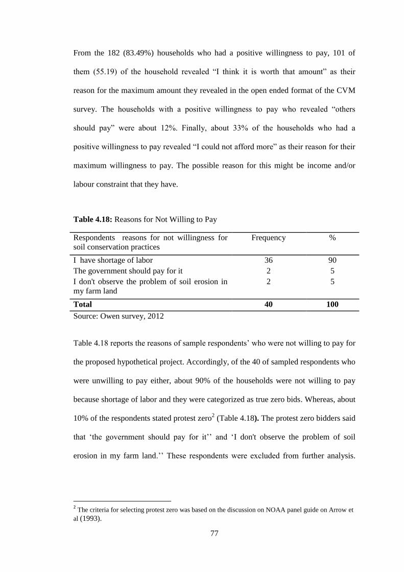
77
From the 182 (83.49%) households who had a positive willingness to pay, 101 of
them (55.19) of the household revealed “I think it is worth that amount” as their
reason for the maximum amount they revealed in the open ended format of the CVM
survey. The households with a positive willingness to pay who revealed “others
should pay” were about 12%. Finally, about 33% of the households who had a
positive willingness to pay revealed “I could not afford more” as their reason for their
maximum willingness to pay. The possible reason for this might be income and/or
labour constraint that they have.
Table 4.18: Reasons for Not Willing to Pay
Respondents reasons for not willingness for
soil conservation practices
Frequency %
I have shortage of labor 36 90
The government should pay for it 2 5
I don't observe the problem of soil erosion in
my farm land
2 5
Total 40 100
Source: Owen survey, 2012
Table 4.18 reports the reasons of sample respondents‟ who were not willing to pay for
the proposed hypothetical project. Accordingly, of the 40 of sampled respondents who
were unwilling to pay either, about 90% of the households were not willing to pay
because shortage of labor and they were categorized as true zero bids. Whereas, about
10% of the respondents stated protest zero2 (Table 4.18). The protest zero bidders said
that „the government should pay for it‟‟ and „I don't observe the problem of soil
erosion in my farm land.‟‟ These respondents were excluded from further analysis.
2 The criteria for selecting protest zero was based on the discussion on NOAA panel guide on Arrow et
al (1993).
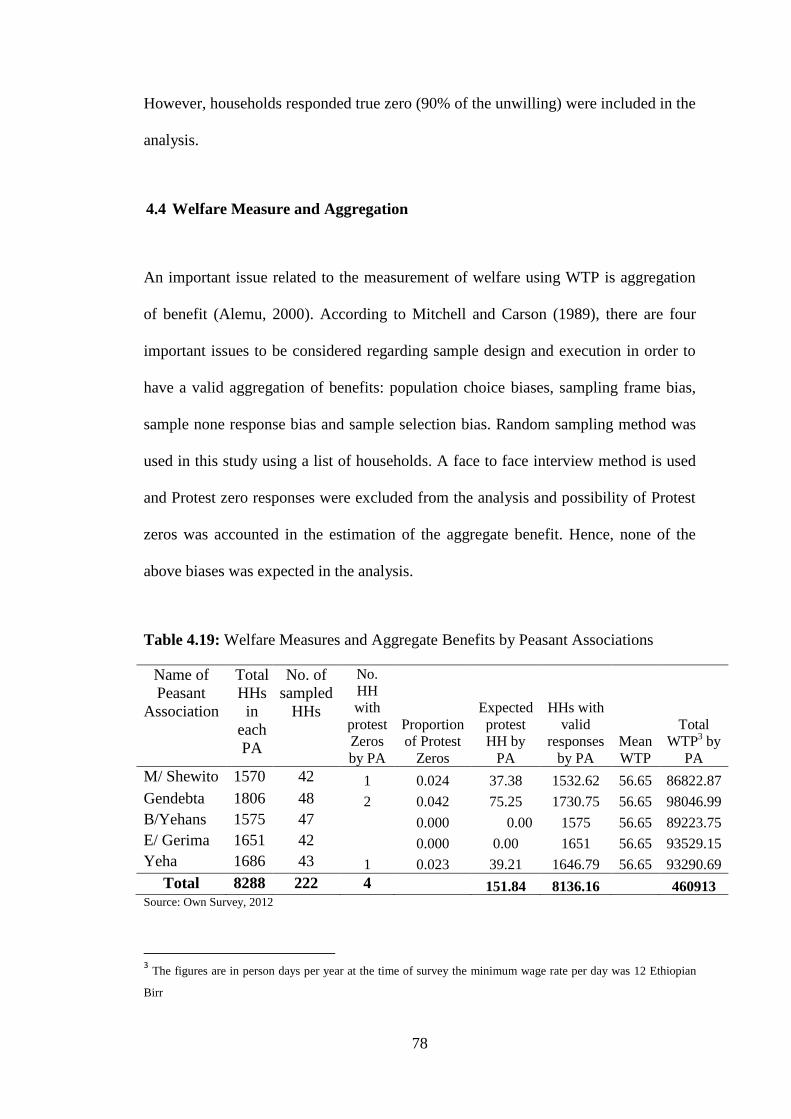
78
However, households responded true zero (90% of the unwilling) were included in the
analysis.
4.4 Welfare Measure and Aggregation
An important issue related to the measurement of welfare using WTP is aggregation
of benefit (Alemu, 2000). According to Mitchell and Carson (1989), there are four
important issues to be considered regarding sample design and execution in order to
have a valid aggregation of benefits: population choice biases, sampling frame bias,
sample none response bias and sample selection bias. Random sampling method was
used in this study using a list of households. A face to face interview method is used
and Protest zero responses were excluded from the analysis and possibility of Protest
zeros was accounted in the estimation of the aggregate benefit. Hence, none of the
above biases was expected in the analysis.
Table 4.19: Welfare Measures and Aggregate Benefits by Peasant Associations
Name of
Peasant
Association
Total
HHs
in
each
PA
No. of
sampled
HHs
No.
HH
with
protest
Zeros
by PA
Proportion
of Protest
Zeros
Expected
protest
HH by
PA
HHs with
valid
responses
by PA
Mean
WTP
Total
WTP3 by
PA
M/ Shewito 1570 42 1 0.024 37.38 1532.62 56.65 86822.87
Gendebta 1806 48 2 0.042 75.25 1730.75 56.65 98046.99
B/Yehans 1575 47
0.000 0.00 1575 56.65 89223.75
E/ Gerima 1651 42
0.000 0.00 1651 56.65 93529.15
Yeha 1686 43 1 0.023 39.21 1646.79 56.65 93290.69
Total 8288 222 4 151.84 8136.16 460913 Source: Own Survey, 2012
3 The figures are in person days per year at the time of survey the minimum wage rate per day was 12 Ethiopian
Birr
79
Mean was used as a measure of aggregate value of soil conservation in this study. The
mean is perhaps better than the median since the good dealt with is not a pure public
good (Alemu, 2000) as there are purely private benefits from soil erosion
conservation measures. In Table 4.19 above, the aggregate WTP was calculated by
multiplying the mean WTP by the total number of households who are expected to
have a valid response in the selected peasant associations. Following this, in this study
the aggregate WTP for soil conservation practices was computed at 460,913
(5,530,956 Birr)4 person days per year for five years in the selected five peasant
associations based on the mean from the double bounded dichotomous choice format.
Whereas, from open ended questions the total WTP for soil conservation practices
was also computed at 398,183.67 (4,778,204.04 Birr) person days per year. This
shows that there is high level of willingness to pay for soil conservation practices in
the study area.
There are 24,692 households in the study area (Adwa Woreda). It is also possible to
calculate the total aggregate value of soil conservation practices for the whole
Woreda. After deducting the protest zeros (445)5 the expected total households with
valid responses are 24,247 households. The total willingness to pay in the whole study
area (Adwa Woreda) is simply the multiplication of the respective means and the
number of expected households to have valid responses. Hence, the aggregate value
of soil conservation in the study area from the double bounded and open ended
4 Is the monetary value of the person day estimates which was multiplied by 12 Birr, the minimum
wage rate in the study area at the time of data collection 5 Those are households‟ which are expected to protest against the proposed project in the entire study
area, Adwa Woreda. It was calculated by the multiplication of the percentage of protest sampled
households‟ (1.8%) by the total number of households in the study area. Hence, 1.8%*24,692 = 445.
This number was deducted from the total number of households in the study area for welfare analysis.
80
formats are 1,373,592 (16,483,104 Birr) and 1,186,648.18 (14,239,778.16 Birr)
person days per annum for five years, respectively.
The purpose of this chapter was to assess the determinants of WTP, to estimate mean
WTP as well as aggregate value of soil conservation practices in Adwa Woreda. The
results of the probit model showed that; Age of the household head (AGE) and Initial
bid offered (BID1) were found to significantly affect WTP decision negatively. On
the other hand, Education level of the household head (EDUCATION), perception of
soil erosion problem (PERCEPTION), Total livestock units (TLU), Sex of the
household head (SEX), Family size of the household (FSIZE) and land tenure
(TENURE) were found to be significant to affect WTP positively. The mean WTP
from the bivariate model estimates and open ended format were found to be 56.65 and
48.94 person days per annum per household for five years. The total aggregate value
of soil conservation practices in the study area from the double bounded and open
ended formats were calculated to be 1,373,592 (16,483,104 Birr) and 1,186,648.18
(14,239,778.16 Birr) person days per annum for five years, respectively.

81
CHAPTER FIVE
5.0 CONCLUSION AND RECOMENDATION
5.1 Conclusion
Soil erosion is one of the most chronic environmental and economic problems of the
present situation in Ethiopia, in general, and in the study area in particular. It is
getting worst than it was ever before. Hillsides stripped of their protective covering of
vegetation are rapidly eroding, depositing huge amount of silt into downstream
reservoirs and river valleys. Floods are becoming more frequent and more sever. To
avert the global as well as local environmental disaster being brought by soil erosion,
it is imperative to take action quickly and on a vast scale. It is therefore, very
necessary to induce in every one‟s mind the importance of conserving soil resources.
To this end, in this study, an attempt was made to analyze local peoples‟ willingness
to pay for soil conservation practices.
The principal objective of this study was to estimate the economic values of soil
conservation measures and to identify and analyze the determinants of farmers‟
willingness to participate in soil conservation practices in Adwa Woreda, Ethiopia.
More specifically, the study was designed to identify the variables, which determine
farmers‟ willingness to participate in soil conservation practices and find out how
each variable is related to the willingness of farmers to participate in soil conservation
practices. Furthermore, the study was designed to see the possibility of cost recovery
by looking at the demand side of the households‟ willingness to pay for soil
conservation practices and to estimate the mean willingness to pay.
82
The study used relevant secondary data and information collected from various
publications, journals and reports but the major sources of data were obtained from a
contingent valuation survey of 218 sample respondents using two stage simple
random sampling technique with structured questionnaire administered with trained
enumerators of Axum University students. Probability proportional to size sampling
technique was employed to select the farm households from five Peasant
Associations, which were selected first by simple random sampling technique.
This study made use of the CVM technique to elicit farmers‟ willingness to contribute
labor for soil conservation practices. Before the final survey was undertaken a pilot
survey was conducted on 30 randomly selected respondents. The open ended format
was used on the pilot survey to come up with the starting bids. A person day of 22, 40
and 65 was used as starting prices in the final survey. In the final survey, the
elicitation method used was double bounded dichotomous choice format with open
ended follow up question.
The chi-square (χ2) test was used to confirm the presence of difference between
acceptance of the offered initial based on the dummy explanatory variables and the F-
Statistics was used for the continuous explanatory variables.
Results of the study revealed that 58.71% of the sampled households were willing to
take the initial offered bid while the rest 41.29% were not willing. However, 83.35%
of the respondents were willing to contribute some amount of labour for the proposed
soil conservation practices. These shows that majority of the households are
concerned about the problem of soil erosion in the study area and there is a possibility

83
of voluntarily instruments such as willingness to pay for soil conservation practices in
the study area.
A probit model was employed to determine the effect of the explanatory variables on
farmers‟ willingness to participate in soil conservation practices. In addition to the
probit model, descriptive statistics were also used to assess farmers‟ perception of soil
erosion problem and to assess WTP for soil conservation practices. Results from
descriptive statistics further showed that the willing and non-willing households
differed significantly in some substantial explanatory variables. The marginal effects
of the explanatory variables were also calculated. Before estimating the models, the
problem of multicollinearity was checked by variance inflation factor (VIF) and
Contingency Coefficient (CC).
Sixteen variables were used on the empirical findings of the determinants of
willingness to pay for soil conservation practices. Age of the household head (AGE)
and Initial bid offered (BID1) were found to significantly affect WTP decision
negatively. On the other hand, Education level of the household head
(EDUCATION), perception of soil erosion problem (PERCEPTION), Total livestock
units (TLU), Sex of the household head (SEX), Family size of the household (FSIZE)
and land tenure (TENURE) were found to be significant to affect willingness to pay
positively.
Besides, a bivariate probit model was used to calculate the mean willingness to
contribute labor of households for the proposed soil and water conservation practices.
The results revealed that the local communities are willing to pay for the proposed
project. The mean willingness to pay from the double bounded dichotomous choice

84
format and open ended format was calculated to be 56.65 and 48.94 person days per
annum, respectively. The aggregate welfare gain from soil conservation in the study
area from the double bounded dichotomous choice format and open ended format was
calculated to be 1,373,592 and 1,186,648.18 person days, respectively.
The study found that the value of soil conservation from open ended format was
underestimated as compared to the double bounded format. This may indicate free
riding and lack of base for answering WTP questions under open ended format. Thus,
in estimating the value of environmental resource like soil conservation at household
level, it is important to use contingent valuation method in the form of double
bounded elicitation format than other elicitation method (that is, open ended
question). In general, the study founds high level of welfare gain from projects of soil
conservation practices in the study area.
5.2 Recommendation
The results of the study have shown that the socio economic characteristics of the
household and other institutional factors are responsible for household‟s willingness
to pay for soil conservation practices. Therefore, policy and program intervention
designed to address soil erosion problems in the study area have needed to take in to
account these important characteristics for effectiveness. Based on the findings of the
study, the following points need to be considered as possible policy implications in
order to enhance farmers‟ participation in the planning and implementation of soil
conservation activities.

85
In order to introduce a sustainable soil management at a household level, the
households should be given the right to play the major role in planning,
managing, controlling and using their own resources. It is also better for the
policy makers to design the participation of the households based on labor
contribution than cash contribution, while designing a soil conservation project.
The results of this study shows that sex of the household head had a positive
effect on willingness to pay decision. This shows that female headed households
are less willing to pay for soil conservation practices than male headed
households. This is because female headed households have limited resource
possessions as compared to male headed households. Hence, there is a need to
enhance the capacity and resources possession of female headed households so
that they can able to take their parts in soil conservation practices as they have
accounted for substantial number in the rural families of the study area.
The level of formal education of the household head was found to be an
important variable affecting the probability of willingness to pay for soil
conservation practices. This underlines the importance of human capital
development in increasing the probability of willingness to pay. The results of
the study also show that those farmers who have perceived soil erosion as a
serious problem were willing to participate in soil conservation practices than
those who do not perceived. This implies that unless planners first increase
farmers‟ recognition of soil erosion hazard, it would be very difficult to
implement effective sustainable soil conservation projects.

86
The results of this study also show that land tenure security is positively and
significantly related to the probability of households‟ willingness to pay for soil
conservation practices. This means as the household head thinks he/ she is
secured his land at least until his life time, the probability of WTP for soil
conservation increases. Therefore, increasing security of land tenure through
land certification would enhance the probability of the WTP of the households
for the conservation practices. Furthermore, the results of the study also reveal
that wealth indicators such as total livestock holdings have a positive effect to
WTP for soil conservation practices in the study area. This implies that for
successful management of natural resources such as soil wealth improving
programs should target the poor so that they would be able to pay.
Finally, this study only analyses the demand side information for soil
conservation practices in the study area. It should also be noted that such studies
should also be complemented by other studies such as comparing cost and
benefit of soil conservation practices.
87
REFERENCES
Aklilu, A. (2002). Households‟ Willingness to Pay for Improved Solid Waste
management: The case of Addis Ababa. MSc. Thesis, Addis Ababa University. Addis
Ababa, Ethiopia.
Alberini, A. and Cooper, J. (2000). Application of Contingent Valuation Method in
Developing Countries. Economic and Social Development Paper. FAO, No. 146,
Rome.
Alebel, B. (2002). Analysis of Affordability and Determinants of Willingness to Pay
for Improved Water Services in Urban Areas, Strategy for Cost Recovery: A Case
Study in Nazreth Town, Ethiopia. MSc. Thesis, Addis Ababa University. Addis
Ababa, Ethiopia.
Alemneh, D. (2003). Integrated Natural Resources Management to Enhance Food
Security: The Case for Community-Based Approaches in Ethiopia. Food and
Agricultural Organization of the United Nation. Environment and Natural Resources
Working Paper No. 16. Rome, Italy.
Alemneh, D. (1990). Environment, Famine, and Politics in Ethiopia: A View from the
Village. Lynne Rienner Publishers, Inc.
Alemneh, D., Shishira, K., Yanda Z., and Johnsen, H. (1997). Land degradation in
Tanzania: Perception from the Village. World Bank Technical Paper, No.370.
Washington, D.C:1-17

88
Alemu, M. (2000). “Valuation of Community forestry in Ethiopia: A Contingent Valuation
Study of Rural Households”, Environment and Development Economics. 5: 289-308
Anemut, B. (2006). Determinants of Farmers‟ Willingness to Pay for the
Conservation of National Parks. The Case of Simen Mountains National Park. MSc.
Thesis, Haramaya University. Haramaya, Ethiopia.
Amemiya, T.(1981). Qualitative Response Models: A survey. Journal of Economic
Literature 19, 1483-1536.
Arrow, K. R., Solow, P.R., Potney, E.E., Leamer, R., Radner, H. and Schuman
(1993). Report of the NOAA Panel on Contingent Valuation. Federal
Register.V.58:4601-4614
Aynalem, A. (Undated). Ethiopia: Population and the Environment. Lesson 4.
Available online at www.EthiodemographyAndHealth.Org
Basarir, A., Sayili, M., and Muhammed, S. (2009). Analyzing Producers‟ Willingness
to Pay for High Quality Irrigation Water. Bulgarian Journal of Agricultural Science,
15 (No 6) 2009, 566-573 Agricultural Academy.
Behailu, W. (2009). Determinant of Adoption Decision of Subsistence Farmers for
Improved Soil and Water Conservation Technologies: The Case of Inebsea Sarmeder,
Estern Gojjam, Amhara Regional State, Ethiopia. MSc. Thesis, Haramaya University.
Haramaya, Ethiopia.

89
Bennett, J.W., and Carter, M. (1993). Prospects for Contingent Valuation: Lesson
from the Southeast Forest. Australian Journal of Agricultural Economics, 37(2), 79-
93.
Berry, L. (2003). Land Degradation in Ethiopia: Its Extent and Impact. A discussion
paper.
Birol, E., Karousakis, K., and Koundouri, P. (2006). Using Economic Valuation
Techniques to Inform Water Resources Management: A Survey and Critical Appraisal
of Available Techniques and an Application. Journal Science of the Total
Environment 365, 105-122
Bojo, J., and Cassells, D. (1995). Land Degradation and Rehabilitation in Ethiopia: A
Reassessment. AFTEA working paper, No.17. Washington DC: World Bank.
Cameron, T. A., and Quiggin, J. (1994). Estimation Using Contingent Valuation Data
from A „Dichotomous Choice with Follow-Up‟ Questionnaire. Journal of
Environmental Economics and Management. 27(3):218-34
Chukwuone, N., and Okorji, C. (2008). Willingness to Pay for Systematic
Management of Community Forests for Conservation of Non Timber Forest Products
in Nigeria‟s rainforest Region: Rob B. Dellink and Arjan Ruijs (eds.), Economics of
Poverty, Environment and Natural- Resource Use, 117-137.

90
Daniel, D. (2002). Soil and Water Conservation Techniques and Strategies for Food
Security and Poverty Alleviation. A Paper Presented in the 12th
ISCO Conference,
Beijing
Demeke, A. (2003). Factors Influencing the Adoption of Soil Conservation Practices
in Northern Ethiopia. Discussion Paper. Institute of Rural Development- University of
Gotteningen.
Demeke, B. (1998). Economics of Soil Erosion and Conservation. Review of Litrature
ans a Dynamic Non-linear Optimization Model with Risk and Uncertainties. A Case
Study for Ethiopia. MSc. Thesis in Environmental Economics. Wageningen
Agricultural University
Dominic, B. (2000). Soil Degradation. ESCAP Environment Statistics Course. A
paper for FAO Report.
Doss, C.R., and Morries, M.L. (2001). How does gender affect the adoption of
agricultural innovations? The case of improved maize technologies. Ghana .Journal
of Agricultural Economics. 25(2):27-39.
Feder, G., Just R.E., and Zilbennan, D. (1985). Adoption of Agricultural Innovations
in Developing Countries: A Survey. Economic Development and Cultural Change, 33
(2), pp. 255 -298.
91
Fikru, A. (2009). Assessment of Adoption Behaviour of Soil and Water Conservation
Practices in the Koga Watershed, Highlands of Ethiopia. MSc. Thesis, Cornell
University.
Gebreegziabher, Z., Kooten, G.C., and Soest, D.P. (2006). Land Degradation in
Ethiopia: What Do Stoves have to Do With It? Contributed Paper Prepared for
Presentation at the International Association of Agricultural Economists Conference,
Gold Coast, Australia, August 12 -18, 2006.
Gebremedhin, B. (2004). Economic Incentives for Soil Conservation In the East
African Countries. ISCO-13th
International Soil Conservation Organization
Conference- Brisbane.
Greene, W. H. (2002). Econometric Analysis. Fifth edition. Macmillan, New York.
Greene, W.H. (1993). Econometric Analysis. Second Edition. Macmillan Publishing
Co., New York, NY.
Gujarati, D.N. (2004). Basic Econometrics. 4th
Edition. McGraw-Hill, Inc.
Haab, T., and McConnell, K. (2002). Valuing Environmental and Natural Resources:
The Econometrics of Non Market Valuation. Edward Elger Publishing Limited,
Glensada House, Montpellier Parade, Cheltenham.
Habtamu, T. K. (2009). Payment for Environmental Services to Enhance Resource
Use Efficiency and Labour Force Participation in Managing and Maintaining

92
Irrigation Infrastructure, The case of Upper Blue Nile Basin. MSc. Thesis, Cornell
University.
Hanemann, M. (1984). Welfare Evaluation in Contingent Valuation Experiments with
Discrete Responses‟. American Journal of Agricultural Economics, 66, 332-41.
Hanemann, M., Loomis, J., and Kanninen, B. (1991). Statistical Efficiency of Double-
Bounded Dichotomous Choice of Contingent Valuation. American Journal of
Agricultural Economics, Vol. 73, No. 4. (Nov., 1991), pp. 1255-1263.
Hicks, J.R. (1943). The Four Consumer‟s Surpluses. The Review of Economic
Studies. Vol.11, No. 1, pp., 31-41.
Holden, S., and Shiferaw, B. (2002). Poverty and land Degradation: Peasants‟
Willingness to Pay to Sustain Land Productivity. In: Barret, C.B., Place, F. and Aboud
A.A. (Eds.). Natural Resources Management in African agriculture, CABI
International.
Hurni, H. (1993). Land Degradation, Famine and Land Resource Scenarios in
Ethiopia. In: Pimentel, (Ed). World Soil Erosion and Conservation. Cambridge
University Press.
Hurni, H. (1988). Degradation and Conservation of the Resources in the Ethiopian
Highlands. Mountain Research and Development, 8(2/3): 123-130.

93
Jalan, J., Somanathan, E., and Chaudhuri, S. (2009). Awareness and the Demand for
Environmental Quality: Survey Evidence on Drinking Water in Urban India. Journal
of Environment and Development Economics 14: 665–692 Cambridge University
Press 2009.
Jonse, B. (2005). Valuing Non-Agricultural Uses of Irrigation Water: Empirical
Evidences from the Abbay River-Basin of the Amhara Regional State, Ethiopia. MSc.
Thesis, Addis Ababa University. Addis Ababa, Ethiopia.
Kadekodi, G.K. (2001). Valuation of Natural Resources: What have we learnt from
Indian experience? Indian Journal of Agricultural Economics. 56(3): 286-312.
Kutrilla, J.V. (1995). The Economics of Natural Environments: Studies in the
Valuation of Commodity and Amenity Resources, Washington, Resources for the
Future.
Marcouiller, D., and S. Coggins (1999). Economic Value of Water: An Introduction.
Boaed of Regents of the University of Wisconsin System Doing Business as the
Division of Cooperative Extension of the University of Wiscinsine-Extention, USA.
Mitchell, R. C., and Carson, R. T. (1989). Using Surveys to Value Public Goods: The
Contingent Valuation Method, Resources for the Future, Washington, DC.
Paulos, A. (2002). Determinants of Farmers‟ Willingness to Participate in Soil
Conservation Practices in the Highlands of Bale: The case of Dinsho farming system
area. MSc. Thesis, Alemaya University. Haramaya, Ethiopia.

94
Peterson, G.L., and Sorg, C.F. (1987). Toward the Measurement of Total Economic
Value. United States Department of Agriculture, Forest Service, Rocky Mountain
Forest and Range Experiment Station. General Technical Report, RM; 148.
Shiferaw, B., and Holden, S.T. (1999). Soil Erosion and Smallholders‟ Conservation
Decision in the Highlands of Ethiopia. World Development 27(4): 739-752.
Shiferaw, B., and Holden, S.T. (1998). Resource Degradation and Adoption of Land
Conserving Technologies in the Ethiopian Highland: A Case Study in Andit Tid,
Northern Shewa. Agricultural Economics. The Journal of International Association of
Agricultural Economists (IAAE), 18(3): 233-247.
Solomon, J. (2004). Contingent valuation of Multi-Purpose Tree Resources: The Case
of Arsi Zone, Ethiopia. MSc. Thesis, Addis Ababa University. Addis Ababa, Ethiopia.
Speelman, S., Farolfi S., Frija, A., D‟haese, M., and D‟haese, L. (2010). The Impact
of the Water Rights System on Smallholder Irrigators‟ Willingness to Pay for Water
in Limpopo Province, South Africa. Journal of Environment and Development
Economics 15: 465–483 Cambridge University Press 2010.
Tegegne, G. (1999). Willingness to Pay for Environmental Protection: An Application
of Contingent Valuation Method (CVM) in Sekota District, Northern Ethiopia.
Ethiopian Journal of Agricultural Economics, 3(1)
95
Tekelu, E., and Gezeahegn, A. (2003). Indigenous Knowledge and Practices for Soil
and Water Management in East Wolega Ethiopia. Conference on International
Agricultural Research and Development. Göttingen, October 8-10.
Teklewold, H., and Kohlin, G. (2011). Risk Preferences as Determinants of Soil
Conservation in Ethiopia. Soil and Water Conservation Society, Journal of Soil and
water Conservation 66(2): 87-96.
Tessema, W., and Holden, S. (2006). Soil Degradation, Poverty, and Farmers‟
Willingness to Invest in Soil Conservation: A case from a Highland in Southern
Ethiopia. Ethiopian Economic Association, Proceedings of the Third International
Conference on the Ethiopian Economy, Vol. 2, pp 147- 164.
Tietenberg, T. (2003). Environmental and Natural Resource Economics. 5th
edition,
Pearson Education, Inc, U.S.A.
Wegayehu, B. (2003). Economics of soil and water conservation: Theory and
Empirical Application to Subsistence Farming in the Eastern Ethiopia highlands. PhD
Dissertation, Swedish University of Agricultural Sciences, Uppsala.
Whittington, D. (1998). Administering Contingent Valuation Surveys in Developing
Countries. World Development. 26(1): 21-30.
Yitayal, A. (2004). Determinant of Use of Soil Conservation Measures by Small
Holder Farmers; in Gimma Zone, Dedo District. An MSc Thesis Presented to School
of Graduate Studies of Alemaya Universtity.
96
Yu, X., and Abler, D. (2010). Incorporating Zero and Missing Responses in to CVM
with Open Ended Biddings: Willingness to Pay for Blue Skies in Beijing.
Environment and Development Economics 15: 535 – 556.
Zewudu, B., and Yemsirach, A. (2004). Willingness-to-Pay for Protecting
Endangered Environment: The Case of Nechsar National Park. Social Science
Research Report.

97
APPENDIX I: Questionnaire
This questionnaire has been prepared to gather information about farming practices,
problem of soil erosion, willingness to pay for soil conservation and socioeconomic
conditions of households. The objective of this questionnaire is to collect information
related to willingness to pay for soil conservation practices in this Woreda. The
research is intended to develop a mechanism to help you in improving land
productivity through soil conservation practices in collaboration with you. The
information that you have delivered to the student will only be used for academic
purposes. In answering my questions, please remember that there are no correct or
wrong answers. I am Just after your opinion. Hence, we request you honest and fair
responses to fill up this questionnaire.
General Information:
Name of the enumerator-------------- Sign. -------------- Date--------------
Name of the PA---------------- Name of the Village------------
FARMER/HOUSEHOLD INFORMATION
1.1. Age_________
1.2. Gender Male = 1 Female = 0
1.3. Marital status
Married =1 Divorced =3
Single =2 Widowed =4
1.4. Education Level---------------------years.
1.5. When did you start farming for your own? (year)______
1.6. Did you have some social position in the community so far? Yes=1 no=2
1.7. If yes, what is your position in the community? ------------------------------------
1.8 . Distance from home to the nearest market..............................Munites?
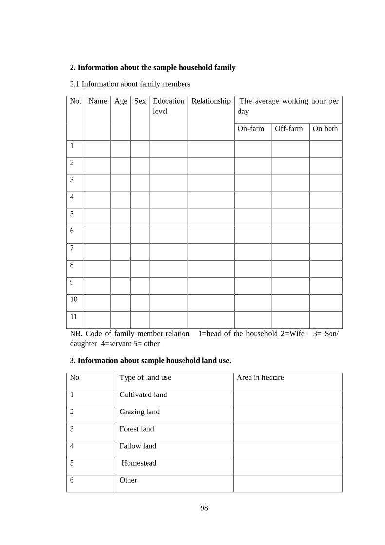
98
2. Information about the sample household family
2.1 Information about family members
No. Name Age Sex Education
level
Relationship The average working hour per
day
On-farm Off-farm On both
1
2
3
4
5
6
7
8
9
10
11
NB. Code of family member relation 1=head of the household 2=Wife 3= Son/
daughter 4=servant 5= other
3. Information about sample household land use.
No Type of land use Area in hectare
1 Cultivated land
2 Grazing land
3 Forest land
4 Fallow land
5 Homestead
6 Other

99
4). AWARENESS TOWARDS EROSION AND EROSION HAZARDS
4.1 Do you perceive the problem of soil erosion in your area? 1.Yes 0. No
4.2 If yes, what features lead you to believe that such problem exists?
(i)----------------------------------------------
(ii) --------------------------------------------
4.3 Is your farmland prone to erosion? 1. Yes 0. No
4.4 If yes, how much of your farmland affected by erosion in (ha)--------------------
4.5 How do you perceive the level of parcel‟s exposure to soil erosion?
1. No risk 2. Medium 3. High exposure to erosion
4.6 Has your farmland been severely affected by soil erosion before?
1. yes 0. No
4.7 If yes, severity of erosion on your farming plots since started farming ?
1. very severe 2. Severe 3. Minor
4.8. When did soil erosion problem start in your farm?
1.Prior to birth (heard from parents) 2. Since childhood
3. In recent years (before ----- years) 4. Others (specify)------------------
4.9. How does the household perceive the soil depth/ fertility since starting farming as
compared to the past?
1. Increasing 2. Decreasing 3. No change 4. Do not know
4.10. If answer is increasing to 9, what measures did the household take to rehabilitate
the conditions?
1. Apply manure 2. Apply chemical fertilizer 3. Practice terracing
4. Planted trees or grass 5. Fallow system 6. Strip cropping along the
contour 7. Bunding 8. Check dams 9. Others(specify)----
4. 11. How serious is the decline in soil fertility on the main plot since started farming
with reference to normal year/ adequate rainfall?
1.Very serious 2. Serious 3.Minor 4. No problem

100
4. 12. Do you think soil erosion will affect your farmland in the future if situations
remain unchecked?
1.yes 0. No
4.13. Slope of the land you have (as perceived by the farmer)
1. Very steep 2. Steep 3. Gentle slope 4.Flat 5. Others (specify)----------
4.14. Have you taken any of the following measures because of erosion?
1. abandoned your cultivated land 2. Expanded to marginal land
3. have taken off farm employment 4. Other (specify)---------
4.15.How is the fertility of your farmland? (As perceived by the farmer)
1. fertile 2. Moderately fertile
3. Infertile 4. Others (specify)--------.
4. 16. If non-fertile, what was the cause of non-fertility?
1. Intensive cultivation for many years 2. Erosion
3. Do not know 4. Others (specify)--------
4.17. Do you observe change in the level of crop yield on your cultivated land?
1. Yes 0. no
5. AWARENESS TO TECHNOLOGY
5.1. Do you know the existence of soil conservation practices?
1.yes 0.no
5.2 . If yes to 1, have you used any one of the following physical soil conservation
practice(s)?
1. Terrace 2. Counter bunds 3. Grass strip 4. Soil and stone bund 5.Others
5.3. If the farmer did not use any soil conservation practice, mention reasons for not
using.
1. lack of money 2. Labor shortage 3. Others (specify)-----------------
5.4. Have you participated in community conservation activities this year?
1. yes 0. No
5.5 Do you use fertilizer on your farm to maintain soil fertility?
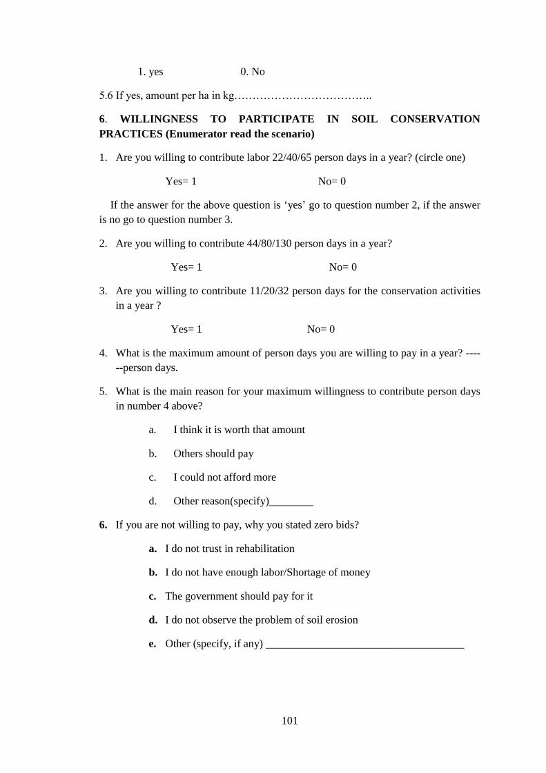
101
1. yes 0. No
5.6 If yes, amount per ha in kg………………………………..
6. WILLINGNESS TO PARTICIPATE IN SOIL CONSERVATION
PRACTICES (Enumerator read the scenario)
1. Are you willing to contribute labor 22/40/65 person days in a year? (circle one)
Yes= 1 No= 0
If the answer for the above question is „yes‟ go to question number 2, if the answer
is no go to question number 3.
2. Are you willing to contribute 44/80/130 person days in a year?
Yes= 1 No= 0
3. Are you willing to contribute 11/20/32 person days for the conservation activities
in a year ?
Yes= 1 No= 0
4. What is the maximum amount of person days you are willing to pay in a year? ----
--person days.
5. What is the main reason for your maximum willingness to contribute person days
in number 4 above?
a. I think it is worth that amount
b. Others should pay
c. I could not afford more
d. Other reason(specify)________
6. If you are not willing to pay, why you stated zero bids?
a. I do not trust in rehabilitation
b. I do not have enough labor/Shortage of money
c. The government should pay for it
d. I do not observe the problem of soil erosion
e. Other (specify, if any) ____________________________________
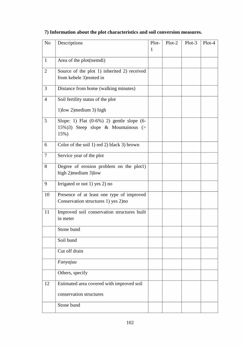
102
7) Information about the plot characteristics and soil conversion measures.
No Descriptions Plot-
1
Plot-2 Plot-3 Plot-4
1 Area of the plot(tsemdi)
2 Source of the plot 1) inherited 2) received
from kebele 3)rented in
3 Distance from home (walking minutes)
4 Soil fertility status of the plot
1)low 2)medium 3) high
5 Slope: 1) Flat (0-6%) 2) gentle slope (6-
15%)3) Steep slope & Mountainous (>
15%)
6 Color of the soil 1) red 2) black 3) brown
7 Service year of the plot
8 Degree of erosion problem on the plot1)
high 2)medium 3)low
9 Irrigated or not 1) yes 2) no
10 Presence of at least one type of improved
Conservation structures 1) yes 2)no
11 Improved soil conservation structures built
in meter
Stone bund
Soil bund
Cut off drain
Fanyajuu
Others, specify
12 Estimated area covered with improved soil
conservation structures
Stone bund

103
Soil bund
Cut off drain
13 When start the construction of improved
soil conservation structure on the plot?
14 Who constructed the structures?
1)Community participation 2) Family
(hired)labor 3) Financial incentives by
government 4)labor exchange
15 Status (degree) of use of improved soil
conservation structures (practices)1)
Removed totally 2) Partially removed3) Not
removed; 4) Modified
16 Who did the maintenance work?
1) Community participation 2) Family/hired
labor 3) labor exchange
17 Traditional soil conservation structures built
(in meter)
Traditional stone bund
Traditional soil bund
Cut off-drain
Traditional ditches
Trash lines
Others, specify
8. LABOUR AVAILABILITY
8.1. Do you have labour shortage for farm activities? Yes =1 no =0
8.2. If yes, for which kind of farm activities?
1. Crop production 2. livestock production
3. Soil conservation activities 4. other (specify)-----------------

104
8.3. If yes to 8.1, how do you solve labour shortage?
Hiring labour =1 use communal labour =2 other (specify)=3---------------------
8.4. If labour is hired, what type of labour do you hire?
Permanent =1 casual =2 both =3
8.5. If permanent, how much do you pay per annum?(birr)______
8.6. If casual, how much do you pay per day?(birr)______
8.7. Can you get labour to hire when you are in need?
Yes =1 no =0
8.8. Do you or your family member work on off- farm activities? 1) Yes 2) No
8.9. If the answer to question 8.8 is yes, Fill in the following table For 2003/04
No
Type of off-farm (non-
farm) activity
Family members working
1)men 2)women 3)children
Total income
obtained in one year
(birr)
1 Pity trade
2 Pottery
3 Weaving
4 Leather making
5 selling of fire wood
6 Labor hire out
7 Remittance
9. INSTITUTIONAL CONTACT AND ASSISTANCE
9.1. Frequency of visit by development workers per year? --------------- days
9. 2. Have you received extension advice on soil conservation practices so far?
1.yes 0. No
9. 3. Are there any governmental or non-governmental organizations working on soil
conservation activities in your area?
1.yes 0.no

105
9. 4. Have you been advised by any of these organizations to undertake soil
conservation practices? 1. Yes 0.no
9.5. In which kind of soil conservation programs have you been involved?
1.food for work 2. Money for work 3. Free 4. Others (Specify)-----------
9.6. Have you attend any soil conservation training in the past?
1. Yes 0. No
10. TENURE OR PROPERTY RIGHT
10.1. For how long have you been with your land? ------------------------
10.2. Do you feel secure that the land belongs to you at least in your lifetime?
1.yes 0. No
10.3. If no, what are the reasons?----------------------------------------------------------------
10.4. How would the newly married member(s) of the household get land?
1. Share the household land 2. The PA provide him/her 3.Other (Specify)
11 . INCOME SOURCE OR WEALTH INDICATORS
11.1. What are your main sources of income (in order of importance)?
crop sale =1 live stock sale =2 Off-farm income =3 others (specify) =4------
11.2. What was the estimated amount of off-farm income in birr (in 2003)?-----------
11.3. If the household does not have more than one ox ask how the household plough
its farm.
1. Rented ox 2. Pairing with others 3. shared out/rent out the land
4. Other (specify)---------------------------
11.4. If the household do not have ox ask how the household plough its farm?
1. Hoe/spade 2. Coupling with others 3. Exchange labour for ox / oxen 4. Rented
ox/oxen 5. shared out/rent out the land 6. fallow the land 7. Others (specify)----

106
A) Please indicate amount of crops produced and sold in this year (2003 EC)
Type of
Crop
Land used For
rain feed
agriculture in
‘tsimdi’ (2003)
Output
in (kg)
Land
irrigation
farming
Output
in (Kg)
For
sells
(kg)
Average
selling
price
Teff
Wheat
Barley
Hanfes
Sorghum
Maize
Beans
Field peas
Faba bean
Pea
Linseed
Lentil
Noug
Tomato
Potato
Garlic
Onion
Cabbage
other
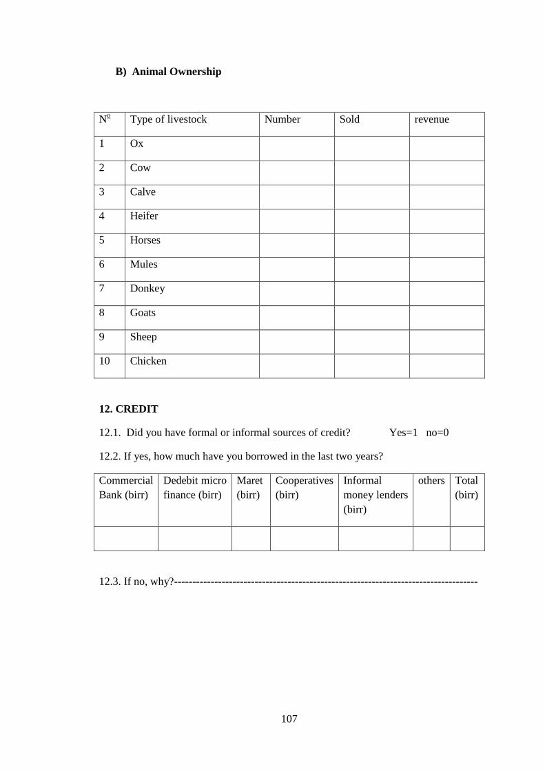
107
B) Animal Ownership
No Type of livestock Number Sold revenue
1 Ox
2 Cow
3 Calve
4 Heifer
5 Horses
6 Mules
7 Donkey
8 Goats
9 Sheep
10 Chicken
12. CREDIT
12.1. Did you have formal or informal sources of credit? Yes=1 no=0
12.2. If yes, how much have you borrowed in the last two years?
Commercial
Bank (birr)
Dedebit micro
finance (birr)
Maret
(birr)
Cooperatives
(birr)
Informal
money lenders
(birr)
others Total
(birr)
12.3. If no, why?-----------------------------------------------------------------------------------
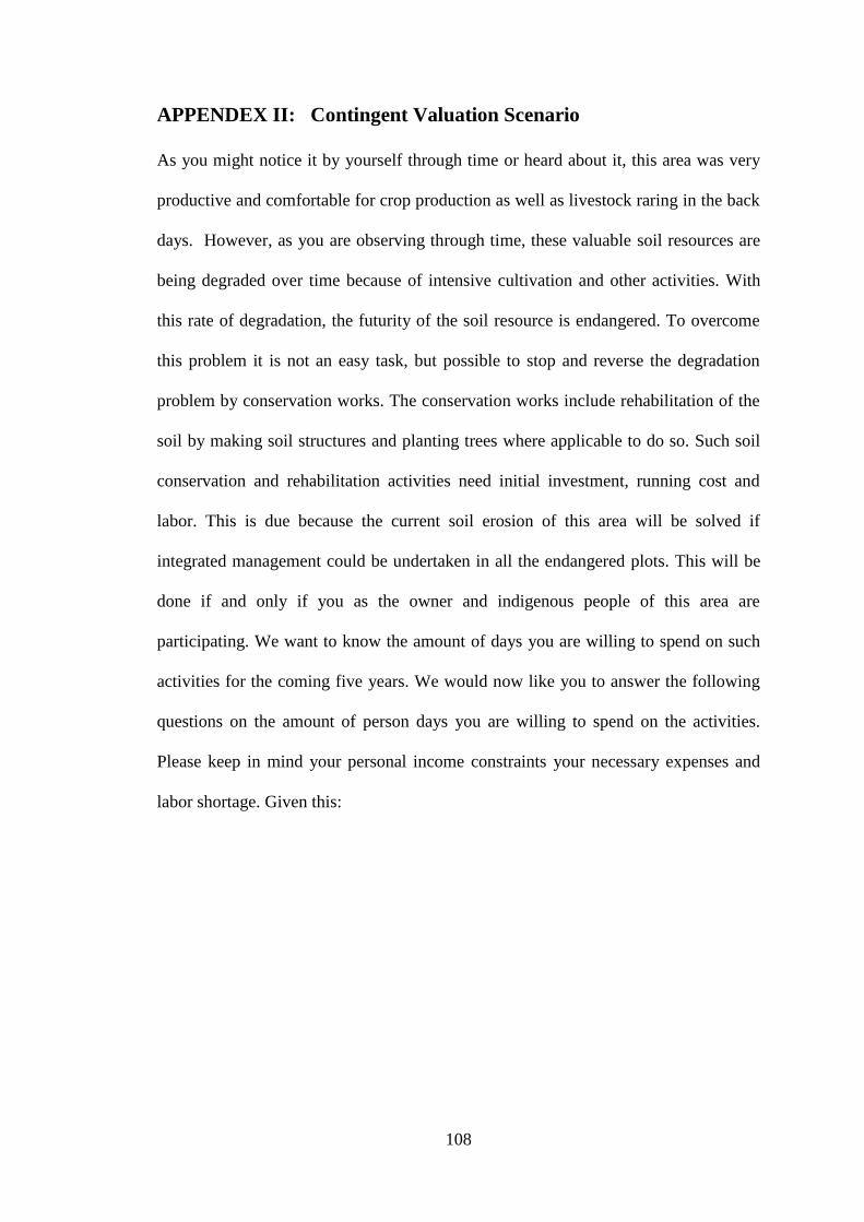
108
APPENDEX II: Contingent Valuation Scenario
As you might notice it by yourself through time or heard about it, this area was very
productive and comfortable for crop production as well as livestock raring in the back
days. However, as you are observing through time, these valuable soil resources are
being degraded over time because of intensive cultivation and other activities. With
this rate of degradation, the futurity of the soil resource is endangered. To overcome
this problem it is not an easy task, but possible to stop and reverse the degradation
problem by conservation works. The conservation works include rehabilitation of the
soil by making soil structures and planting trees where applicable to do so. Such soil
conservation and rehabilitation activities need initial investment, running cost and
labor. This is due because the current soil erosion of this area will be solved if
integrated management could be undertaken in all the endangered plots. This will be
done if and only if you as the owner and indigenous people of this area are
participating. We want to know the amount of days you are willing to spend on such
activities for the coming five years. We would now like you to answer the following
questions on the amount of person days you are willing to spend on the activities.
Please keep in mind your personal income constraints your necessary expenses and
labor shortage. Given this:
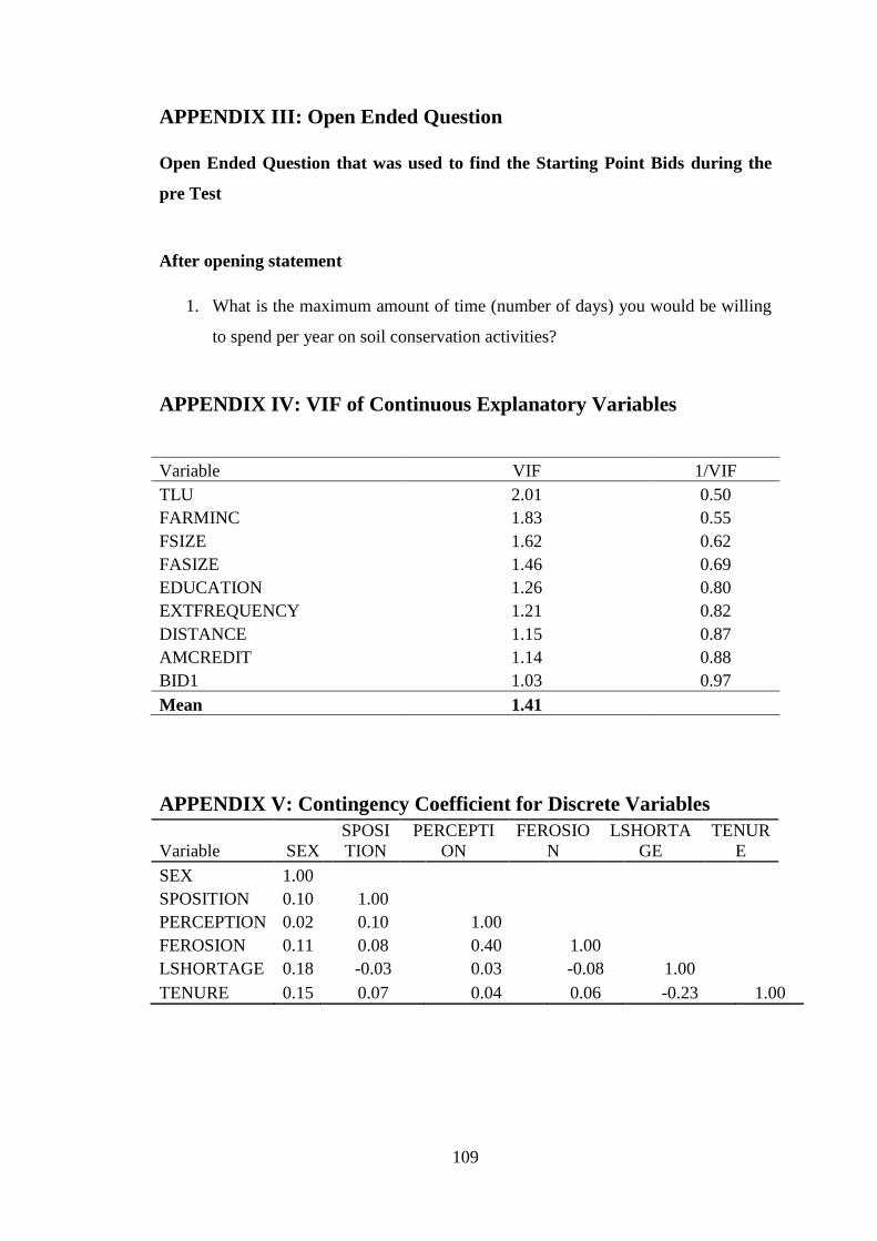
109
APPENDIX III: Open Ended Question
Open Ended Question that was used to find the Starting Point Bids during the
pre Test
After opening statement
1. What is the maximum amount of time (number of days) you would be willing
to spend per year on soil conservation activities?
APPENDIX IV: VIF of Continuous Explanatory Variables
Variable VIF 1/VIF
TLU 2.01 0.50
FARMINC 1.83 0.55
FSIZE 1.62 0.62
FASIZE 1.46 0.69
EDUCATION 1.26 0.80
EXTFREQUENCY 1.21 0.82
DISTANCE 1.15 0.87
AMCREDIT 1.14 0.88
BID1 1.03 0.97
Mean 1.41
APPENDIX V: Contingency Coefficient for Discrete Variables
Variable SEX
SPOSI
TION
PERCEPTI
ON
FEROSIO
N
LSHORTA
GE
TENUR
E
SEX 1.00 SPOSITION 0.10 1.00
PERCEPTION 0.02 0.10 1.00 FEROSION 0.11 0.08 0.40 1.00
LSHORTAGE 0.18 -0.03 0.03 -0.08 1.00 TENURE 0.15 0.07 0.04 0.06 -0.23 1.00