Housing Activity and Consumer Spending

Jonathan McCarthy and Charles Steindel∗

Macroeconomic and Monetary Studies Function Federal Reserve Bank of New York

Abstract. The current expansion has seen record-high levels of transactions in housing, extraordinary growth in the aggregate value of owner-occupied housing, and large increases in the amount of funds realized from the refinancing of mortgage debt. Many analysts thus have pointed to the strong housing market and rising home prices as a major pillar supporting recent economic growth and have expressed concern that a contraction in housing activity and values could pose a significant risk to consumer spending and real economic growth. This paper explores the channels by which the housing market may affect consumer spending and assesses the potential risk from a softening in the housing market. Our assessment is that a housing slowdown by itself may slow consumer spending some; however, it is probably insufficient to precipitate a downturn without some additional shocks outside of the sector.

∗ The views expressed in this paper represent those of the authors alone and not necessarily those of the Federal Reserve Bank of New York or the Federal Reserve System.

1

Introduction

The current expansion has seen record-high levels of transactions in housing, extraordinary growth

in the aggregate value of owner-occupied housing, and large increases in the amount of funds realized from

the refinancing of mortgage debt. At the same time, the macroeconomic data show that consumer spending

has played a large role in recent economic growth. The simultaneity of these developments has suggested

to many analysts that the strong housing market and rising home prices have been a major (if possibly

unsustainable) pillar supporting the economy. Moreover, many of these analysts are concerned that a

contraction in housing activity and values, if it occurred, could pose a significant risk to consumer

spending, accentuating the direct effect from a fall-off in residential construction.1

This paper explores the channels by which the housing market may affect consumer spending and

assesses the potential risk to aggregate activity through these channels from a softening in the housing

market. The channels we examine include the following. (1) The direct mechanical relationship between

housing and consumption; i.e., some components of consumer spending are complementary to housing

transactions. (2) The “wealth effect” from capital gains on housing. (3) The role of greater home equity

extraction—stemming from less costly mortgage refinancing and more accessible home equity loans—on

recent household spending behavior.

Our assessment is that a housing slowdown by itself may slow consumer spending and GDP

growth some; however, it is probably insufficient to precipitate a downturn without some additional shocks

outside of the sector. First, the amount of consumer spending more or less mechanically tied to housing

transactions is fairly limited. Second, while the precise size of the wealth effect from gains in home prices

is problematic, plausible estimates do not suggest that consumer spending growth would cease if there was

a decline in home values on the order of recent gains. Third, it appears that much of the recent home equity

withdrawal has been used to restructure household balance sheets as well as to finance consumer spending

decisions based on fundamental consumption determinants (such as expected income growth) rather than

on the availability of this source of funds.

The next portion of the paper reviews the basic facts on housing activity, aggregate home values,

and the recent evolution of household wealth and spending. We then examine and assess the consumer

1 An extreme version of these concerns is expressed in Baker (2006).

2

spending impact of housing activity through the channels listed above. The last section provides

concluding remarks.

Recent Trends in Housing, Household Wealth, and Spending

The two aspects of housing activity directly linked to real economic activity are construction and

sales. Within the national income accounts, the data on home construction are contained in the residential

investment component. This component consists of all outlays on home construction—renovations and

improvements, as well as new building of single and multifamily structures. It also includes the value

added in the course of home sales, which is approximated by fees earned by real estate brokers.

Residential investment has risen briskly in this expansion. The annual rate of increase in real

residential investment from the start of 2002 through 2006Q1 has been 7.9 percent, more than twice that for

GDP as a whole. Nonetheless, this growth pace is about the same as that for the corresponding period of

the expansion of the 1990s and is well below the gains seen in prior expansions. Residential investment on

average contributed about 0.4 percentage point to overall GDP growth over 2002Q1 to 2006Q1 (Chart 1).

This is a somewhat larger growth contribution than in the comparable period of the 1990s expansion, but

less than in the economic expansions of the 1970s and 1980s.

Although the recent growth rate of residential investment has not been unusual, the level of

housing market activity has been extraordinary. This reflects the fact that the recent expansion of

residential investment has occurred without a significant bust preceding it. Consequently, the share of

residential investment recently exceeded 6 percent of GDP, its highest since early 1950s (Chart 2). Other

measures of single family housing activity have set new records. Single-family housing starts have

exceeded its previous peak (set in December 1977) several times in the past few years, with the January

2006 figure of 1.843 million units (annual rate) the current peak. Home sales also have set new highs

during the recent expansion: the current peak of new homes sales is 1.371 million units (annual rate) in July

2005 and the current peak of existing home sales is 6.33 million units in June 2005. The decline in sales

since these peaks has prompted some of the concern about a slowing housing market and its possible

spillovers to the rest of the US economy.

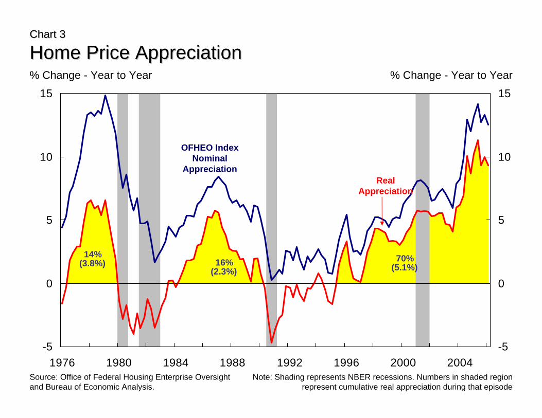
The other extraordinary feature of housing market in recent years has been the rise in home prices.

The four-quarter change in the repeat sales index compiled by the Office of Federal Housing Enterprise

3

Oversight (OFHEO) has exceeded 10 percent since 2004Q2, the first time this has occurred since the high

inflation late 1970s (Chart 3). More impressively, real home prices have increased steadily since 1995.

The length of the real home price boom and its cumulative size is unprecedented in the history of the

OFHEO series. On a longer perspective, the data in Shiller (2006), which starts in 1890 for the US,

indicates that the recent rise in real home prices is unusual.

This rise in real home prices has sparked considerable debate about whether there is a “bubble” in

home prices.2 An analysis of this issue is beyond the scope of this paper, but it is sufficient to note that for

most of the issues we address, the answer to the bubble question is not particularly relevant; that is, the

source of a home price decline will have only a little impact on the effects of that decline on consumer

spending, unless the home price decline is associated with a significant change in households’ longer-term

attitudes.

The brisk pace of residential investment and the strength in housing prices have swelled the value

of homes in the household balance sheet. According to the Federal Reserve Board’s Flow of Funds data,

the aggregate value of residential real estate owned by U.S. households was almost $20 trillion at the end of

2005, accounting for over 30 percent of all the assets owned by the household sector (Chart 4).3

Mortgage indebtedness has grown in tandem with the value of housing. This is one factor behind

the rise in the leverage in the household sector: the ratio of aggregate household debt to aggregate

household assets of 18.5 percent in 2006Q1 roughly matches that of the previous two quarters as the

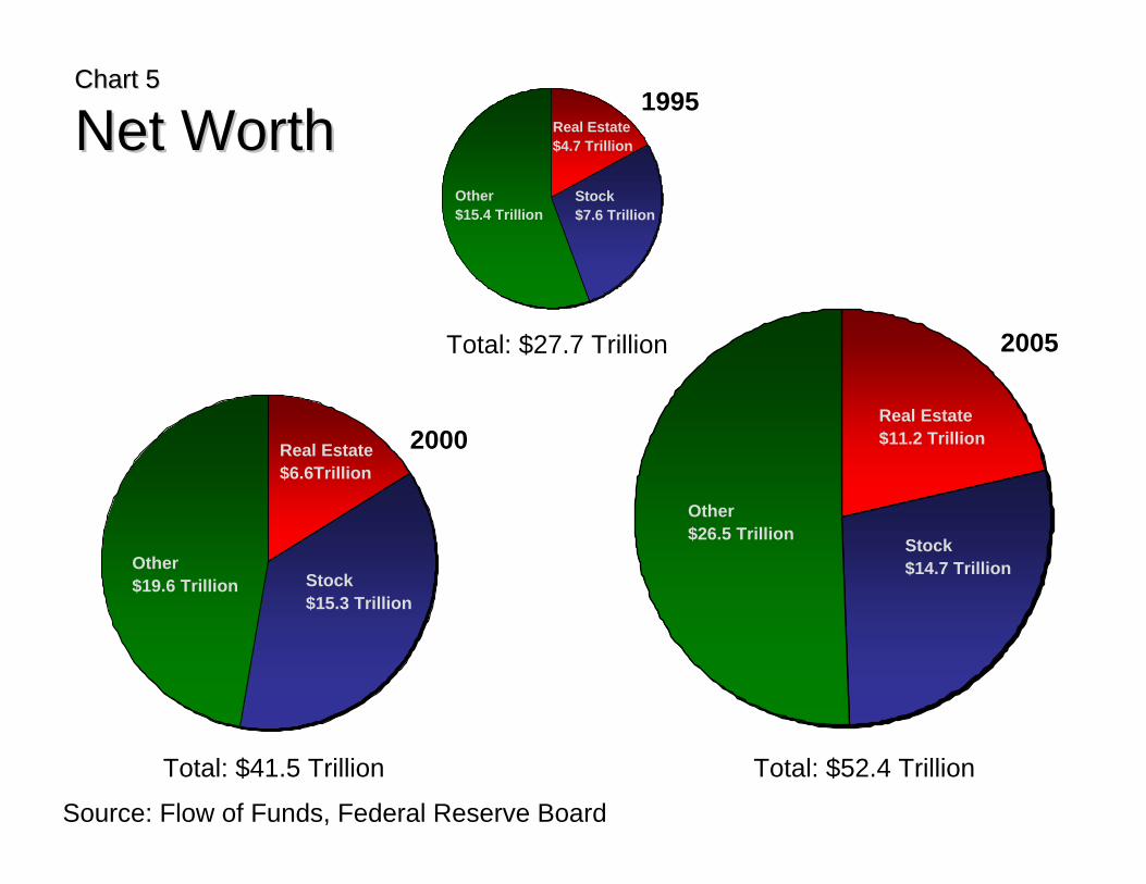
highest historical value of this ratio. Nonetheless, the owners’ equity share of residential real estate has

been little changed in the past three years at around 56%. The dollar value of equity in residential real

estate increased by more than $1 trillion in each of the last two years and was above $11 trillion at the end

of 2005. Owners’ equity of real estate comprised 21.4 percent of household net worth (which totaled over

$52 trillion) at that time, its highest share since 1989 (Chart 5).4

2 Some papers have argued that housing market “fundamentals” (particularly the long-term decline in interest rates) can explain the recent rise in real home prices; see, for example, McCarthy and Peach (2004) and Himmelberg, Mayer, and Sinai (2005). Of course, a number of other analysts have claimed that only nonfundamental factors could explain the extent of the rise. For recent examples, see Baker (2006) and Shiller (2006). 3 Household real estate assets were $20.4 trillion as of the end of 2006Q1. 4 The net worth of household real estate was $11.4 trillion at the end of 2006Q1, which was 21.2 percent of household net worth of $53.8 trillion.

4

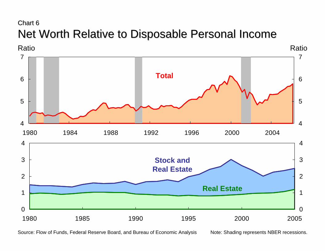
The strength of home values cushioned the impact of the 2000-2002 stock market decline, and,

afterwards, with the stock market recovering, the ratio of household net worth to disposable personal

income had risen to almost 580 percent by the end of 2006Q1. This figure was higher than any earlier

ones, except for those seen in 1998-2000 at the height of stock market values (Chart 6). Although much of

the volatility in the wealth-income ratio reflects stock market swings, an important component of the

longer-term rise has been the surge in housing values. The ratio of owners’ equity in residential real estate

to income grew from less than 90 percent to more than 120 percent between 2000 and 2006Q1.

Along with strength in housing activity and values, this expansion has seen sustained forward

momentum in consumer spending, but it has not been the case that consumer spending has been unusually

strong. Real consumer spending contributed an average of about 2¼ percentage points to overall GDP

growth in 2002-2006Q1. This contribution was slightly smaller than in the comparable period of the

expansion of the 1990s, and considerably smaller than that in the 1980s. However, the recent strength of

consumption has occurred in an environment of very low and declining personal saving; indeed, the

personal saving rate fell below zero in 2005 (at least for the currently reported data). The combination of

well-maintained consumer spending, low personal saving, and remarkable gains in home values (along with

high levels of residential investment) has naturally raised a belief that the latter has contributed to the two

former phenomena. A consequence of that belief and these observations is a concern of some analysts that

a decline in housing activity and home values will lead to a substantial decline in consumer spending and

increase the risks to the macroeconomic environment.

Housing and Consumer Spending: Direct Linkages

A portion of consumer spending appears complementary to housing activity. This portion

includes expenditures directly tied to transactions in housing markets, such as moving expenses, and

spending often associated with home purchase, such as expenditures on furniture, home furnishings, and

major appliances. We examine the relationship between these expenditures and home sales to assess the

implications of housing market fluctuations on this housing-related spending.

5

We use the detailed data on consumer expenditures in the national income accounts to compute

the dollar and real volume of these aggregated expenditures.5 To assess the relationship between this

aggregate and housing activity, we use a Granger causality test of growth rate of these expenditures with

the growth rate of new and existing home sales.6 The results of these tests are in Table 1; they indicate that

home sales Granger cause these expenditures and vice versa (upper panel). In contrast, home sales do not

Granger cause overall consumer spending nor vice versa (lower panel). One can interpret (even though

any such conclusion based on this reduced form is tentative at best) the dual causality for housing-related

expenditures and home sales as suggesting that a third factor contributes to the relationship. In any event,

these results are consistent with our intuition.

Although the linkage between these expenditures and home sales is reasonably firm, the potential

spillover from a slowing housing market probably would not be substantial because these purchases are a

relatively small share of consumer spending. In 2005 aggregate outlays on these products were slightly

under $200 billion, or less than 2½ percent of total consumption. These expenditures have risen robustly in

real terms in recent years (5 to 10 percent), but their small share implies that they have had a small

contribution to real GDP growth, typically on the order of 0.1 percentage point per quarter. As such, a

reversal in the path in these expenditures probably would reduce real GDP growth by a small amount—

maybe ¼ percentage point at most. Still, this drag would reinforce the impact of a contraction in residential

investment.

The Housing Wealth Effect

Much of the emphasis on the effects of housing on economic activity relates to the possible

connections between home price appreciation and consumer spending. Two interrelated channels have

been articulated. The first is a straightforward connection between housing wealth and spending. The

second is a connection between borrowing against home equity and spending. In this section, we consider

the wealth channel.

A simple theoretical framework

5 In particular, we include expenditures on furniture, major appliances, floor coverings, other durable house furnishings (window treatments, etc.), and moving and storage expenses. 6 Granger causality means that lagged movements in home sales precede movements in these expenditures not explained by their own lagged movements.

6

The standard economic framework to analyze consumption has been the life-cycle/permanent-

income model.7 In the model, households make their spending decisions taking into account their expected

lifetime resources, which include current and expected future labor income (“human wealth”) as well as

current net worth (“non-human wealth”). An implication of the model is that when the expected value of

their resources rises, households will increase their consumption, even when current income has not risen.

In particular, increases in net worth, including that from rising home values, will lead to higher spending.

Although the basic logic that changes in wealth may affect spending is fairly straightforward, the

size of that effect is more uncertain. In this simple model, an “exogenous” increase in current wealth

(whether in housing or corporate equities) would lead households to raise their consumption by roughly the

annuity value of the wealth increase. This in turn is related to life expectancy, expected interest rates,

expected future income, and preferences for current spending versus future outlays. A back of the envelope

calculation would suggest that the propensity to consume from wealth gains would be somewhere between

0.025 and 0.05, with the higher number being consistent with households planning to spend the bulk of

their resources over their remaining lifetime.8 Given recent gains in home values, such propensities to

consume would lead to sizable effects on consumption. Capital gains on household real estate assets

amounted to over $2.1 trillion in 2005 according to the Federal Reserve Board’s Flow of Funds:

propensities to consume between 0.025 and 0.05 would imply that consumption in 2005 was about $53-

$107 billion higher than if there were no increases in real estate values. These values equal about 0.6-1.2

percent of total consumption expenditures. A reversal of some of these gains then would imply notably

lower consumption growth.

However, casual observation of wealth fluctuations and consumption suggests that households do

not adjust consumption immediately in response to wealth fluctuations to the extent implied by the simple

model. For example, it does not appear that consumption experienced a boom during the 1990s

commensurate with the stock market boom, nor did spending crash as the stock market declined

7 Friedman (1957) introduced the permanent income model while Ando and Modigliani (1963) is an early example of the life cycle model. Although the models differ in some aspects, they share a basic premise that households make their consumption decisions by maximizing utility subject to an intertemporal budget constraint. As such, the models have been used interchangeably at least since Hall (1978). 8 An estimate of 0.05 would appear consistent with a seemingly low life expectancy of 20 years. However, the bulk of wealth is owned by older households. Moreover, interest earned from wealth enables households to spend a bit more than life expectancy considerations alone would allow.

7

precipitously in 2000-02 (despite the fears of such at the time). There are at least two different ways to

interpret such observations.

One possibility is that households adjust their consumption profile slowly, perhaps because of

intermittent planning periods, the costs of determining the new optimal consumption profile, or other

behavioral considerations. In such a case, the immediate impact of a change in wealth may be small but the

ultimate effect would be as predicted by the model.9 This scenario then would imply that including lagged

values of wealth or an error correction mechanism in estimated consumption functions would be necessary

to determine the size of the ultimate wealth effect, which traditionally has been done in many

macroeconometric models.

Another possibility is that changes in wealth have differential effects on spending depending upon

their ultimate source. A statistical examination of the aggregate data suggests that the propensity to

consume from wealth is not stable (Ludvigson and Steindel, 1999; Steindel, forthcoming); for instance, it

appears to have been low during the stock market boom and in the period thereafter. A plausible

explanation for this instability emerges from a closer look at the basic model of spending. Essentially, the

life-cycle/permanent-income model assumes that households take into account the likely profile of

resources over their planning horizon. If they perceive a current wealth gain as not “sustainable” (in a

sense made more precise below), then they will not increase consumption as much as they would if they

perceived the wealth gain as “permanent” or sustainable.

The framework of Lettau and Ludvigson (2004) provides a more technical explanation for these

statistical results. Their analysis shows that consumption, asset wealth, and labor income are cointegrated,

or share a common long-run trend, which is consistent with the premises of the household lifetime resource

constraint. In their model, shocks to the variables of the system are of two types: “permanent” shocks

affecting the common trend of these variables (these largely reflect changes in the expected growth path of

the economy; in part, these can be thought of as expected changes in productivity growth) and “temporary”

shocks having no effect on the common trend. Lettau and Ludvigson find that consumption fluctuations

are related mostly to permanent shocks; in contrast, wealth fluctuations largely are associated with

temporary shocks. Consequently, only wealth fluctuations related to permanent shocks have any

9 Analysis consistent with this view is presented in Davis and Palumbo (2001).

8

substantive effect on consumption. Wealth effects then depend upon the source of wealth fluctuations: if

permanent, then the effect is about the rule of thumb we discussed above; if temporary (like most wealth

fluctuations), then the effect is very small. Ludvigson (2003) documents how this decomposition accounts

for the low propensity to consume from wealth during and after the stock market boom. Essentially,

consumers appeared to regard only about half the run-up in wealth from 1995 to 2000 as “permanent.”

Beyond these considerations about the size and speed of wealth effects, there also is considerable

evidence that some households may not follow the prescriptions of the standard life-cycle/permanent

income model, potentially impacting estimated wealth effects. One reason for this behavior is that some

households probably face liquidity constraints; i.e., they can not finance spending they would otherwise be

willing and able to do. This observation underlies the “buffer stock” models of consumption that have been

used in many recent studies.10 In such models, the propensity to consume out of current resources

(including asset wealth) is higher for constrained households; as such, increases in the wealth of those

households, no matter what the cause, would raise consumption more than it would for unconstrained

households and conceivably imply a larger aggregate effect than suggested by theory.

Another reason that some households may not follow the prescriptions of the standard life-

cycle/permanent-income model is that they determine spending according to a simple rule of thumb, such

as consuming a fixed portion of current income and a fixed portion of wealth gains regardless of the

implications of those changes for lifetime resources (Campbell and Mankiw, 1989). Such behavior may

reflect limited ability or resources to plan the consumption path according to the dictates of the standard

model. Because the rule of thumb for spending out of wealth increases may be higher than the propensity

to consume from wealth implied by the standard model, wealth gains may have a larger effect on aggregate

consumption depending upon the proportion of such households.

Why housing could be different

The above discussion tacitly assumes that all changes in household wealth have comparable

effects on spending. If housing is inherently similar to other forms of wealth, then we could appeal to the

general wealth effects literature to determine its effect on consumer spending. Implicitly, those analysts

that have given housing a more prominent role in sustaining consumption in recent years assume that it is

10 A couple of prominent early examples are Deaton (1991) and Carroll (1997).

9

different from other forms of wealth in regard to its effects on aggregate consumption. Moreover, many of

these analysts also appear to assume that developments in the housing and mortgage markets have led to

the effect of housing wealth on consumption becoming greater in recent years. Some possible reasons for

these views are the following.

Housing is more widely and evenly distributed.

According to survey data, including those collected during the late 1990s stock market boom, for

most American households their home is the most important asset they own (Tracy, Shroeder, and Chan

(1999)). This pattern continues in more recent data. The 2004 Survey of Consumer Finances found that

69.1 percent of families owned their primary residence; for the bottom income quintile, the percentage was

41.6 percent (Bucks, Kennickell, and Moore (2006)). In contrast, 48.6 percent of families held corporate

equity either directly or indirectly; for the bottom income quintile, this percentage was 11.7 percent.

Clearly, the ubiquity of home ownership means that fluctuations in home values could affect the

net worth of a larger portion of the population than fluctuations in other asset prices. Consequently,

assuming that home price fluctuations do affect the spending decisions of homeowners, changes in

aggregate home values will influence spending across a wide swath of the nation. However, widespread

exposure to home price changes does not necessarily imply that the aggregate dollar or real volume of

spending influenced by these changes will be necessarily larger than for equivalent changes in the value of

other assets that are less evenly held. Although the marginal propensity to consume out of wealth in the

standard model can in principle vary according to the level of wealth and income (depending upon the

exact parameterization), in most standard implementations of the model it is not very sensitive to wealth

levels (i.e., consumption is approximately linear in wealth). Consistent with this, there is very little

evidence in microeconomic data that the spending effect of a wealthy family losing $1 million is

substantially smaller than that of 10 middle-class families each losing $100,000.

A differential effect of housing wealth fluctuations on consumption would then appear to depend

upon the extent of the previously described complications to the standard model. In particular, because

housing wealth is more widely held, its fluctuations may affect more liquidity-constrained households than

fluctuations in other assets. If so, then the housing wealth effect may differ from that of other assets.

10

In assessing the impact of housing on consumption in the current situation, there is some basis to

believe that this avenue for a differential impact from housing may have a lesser influence than suggested

by the data on the holding distribution of the assets. In particular, recent home price appreciation appears

to have been concentrated in high-value homes in high-income areas. We illustrate this in Chart 7, which

plots (log) state per capita personal income in 2000 against state home price appreciation between 2001Q1

and 2006Q1 according to the OFHEO index. The chart shows that most of the high-appreciation states also

have higher income: the included regression line is positively (and statistically significant) sloped.11

Therefore, the recent increase in housing wealth has been unequally distributed, with the previously well-

to-do getting a disproportionate portion.12 Correspondingly, if a correction occurs in the segments of the

market that have seen the greatest increases these same individuals would experience setbacks. Another

way to think of this is that the recent run-up in housing is to some extent comparable in its distribution to

that of typical stock market expansions.

Housing is primary collateral for household loans.

The simple life-cycle/permanent income model implicitly assumes that households are able to

borrow at the risk-free rate without having to post collateral. In reality, much of household debt is

collateralized with real estate. According to the Flow of Funds, over 72 percent of total household

liabilities at the end of 2005 were home mortgages (including home equity loans). Moreover, the home

mortgage share has been rising rapidly over the past five years as more households have become

homeowners and existing homeowners extracted equity from their homes (Chart 8).

The fact that much of household borrowing is backed by real estate collateral suggests that

“financial accelerator” effects may influence the relationship between home values and consumption.13

Although much of the early literature on the financial accelerator had concentrated on its possible effects

on firms, some recent papers have explored how it may affect household behavior and consumption; see,

for example, Aoki, Proudman, and Vlieghe (2004) and Iacoviello (2004, 2005).

11 The slope of the line is 98.1 with a standard error of 23.2, for a t-statistic of 4.24. The R2 of the regression is 0.27. 12 Also see Himmelberg, Meyer, and Sinai (2005) for further evidence on this point. 13 See Bernanke, Gertler, and Gilchrist (1999) for more on this mechanism within a small general equilibrium model.

11

In these models, the borrowing capacity of agents is a function of their “collateralizable” assets;

for households, the empirical data suggest that this is largely the value of their homes. Consequently,

fluctuations in home values would affect the borrowing capacity of households and the availability of loans

to them. This in turn affects the consumption of households that are constrained; i.e., if unsecured loans at

the risk-free rate were available, they would prefer to borrow more to consume. If a significant portion of

spending was done by households whose availability to credit can fluctuate, such shifts in credit availability

then would affect aggregate consumption.

In the current environment of rising home prices, households may have gained from a “virtuous

circle” where the increase in prices raises loan availability, which increases the consumption of previously

credit-constrained households, which in turn supports continued economic strength and further increases in

home prices. However, this effect is dampened as fewer households remain credit-constrained as home

values and borrowing capacity increases. In contrast, if prices begin to fall, the virtuous circle becomes a

vicious circle: prices fall, loan availability declines, consumption declines weakening the economy, and

home prices fall further in response. In addition, the vicious circle is amplified over time as more

households become constrained as loan availability declines. Beyond that, sales by lenders of repossessed

collateral could further depress the market, which would further worsen the cycle.

Iacoviello (2004) presents evidence showing that the behavior of aggregate consumption in the US

is consistent with a version of the financial accelerator model. He estimates that the fraction of

consumption by constrained households is between 0.18 and 0.26 (depending upon the instruments used in

the estimation).14 If a similar fraction of current consumption is by constrained households—the

developments since 2003 may suggest that it is somewhat smaller—this indicates that a substantial fraction

of consumption may be at risk because of financial accelerator effects from a decline in home values.

Moreover, if there has been a sizable increase over recent years in the fraction of homeowners that are

extremely leveraged (as suggested by anecdotal reports of 100-125 percent LTV mortgages), then the risk

could be greater.

However, on a more sanguine note, the aggregate U.S. household sector retains quite substantial

home equity cushions, as noted above. So even if there was a large 10 percent reduction in the value of

14 The estimation period in his regression is 1986:1-2002:4.

12

residential real estate, it would result in the owners’ equity share declining from 56 to 51 percent, a level

that still appears to be substantial. Thus, while there is a potential for the access to credit to become more

restricted to some in case of a major correction in home values, in the aggregate it appears that most U.S.

households would not necessarily move to a fundamentally weaker financial condition and jeopardize their

access to credit.

Housing has become more liquid.

The developments in the mortgage market since the early 1980s have reduced the costs of

borrowing against and increased the liquidity of home equity.15 Moreover, households increasingly have

taken advantage of such opportunities, as we discuss in more detail below. As such, housing has become

more liquid over this period. Traditionally, one motivation for households to own liquid assets has been the

need for precautionary savings to self-insure against hard times. With home equity becoming more liquid,

households may have reduced previously accumulated precautionary savings reserves.16 The unfolding of

this process could have boosted the growth of consumer spending.

Presumably, such a transitional process would dissipate, and consumption growth would return to

a “normal” pace once households realign their portfolios. However, in an environment of rising home

prices and the use of home equity as precautionary assets, households may find that their precautionary

savings are above desired levels (particularly for “buffer stock” households). In such a case, the rise in

home values may induce more consumption than there would be otherwise. Conversely, a decline in home

prices may drop precautionary savings below desired thresholds. This in turn may lead households to cut

spending to accumulate precautionary savings balances in more traditional forms, lowering consumption

more than it would otherwise.

15 McCarthy and Peach (2002) discuss the evolution of the mortgage market during the post-war period from the savings and loan-dominated “New Deal” system to the current capital market based system. To illustrate the decline in mortgage costs, according to the Freddie Mac Primary Mortgage Market Survey, fees and points on a 30-year fixed rate mortgage have declined from about 2.5% in 1985 to 0.5% in 2006. For a 15-year fixed rate mortgage (a more popular refinancing instrument), fees and points have declined from about 1.7% in 1992 (the data for this begin in late 1991) to 0.5% in 2006. 16 McCarthy (1995) noted that in the PSID data he examined from the mid-1980s (when refinancing and home equity loans were less prevalent) households appeared to regard home equity as illiquid and not available for use as precautionary savings. More recently, Hurst and Stafford (2004) found that, using PSID data from the early 1990s, liquidity-constrained households were more likely to refinance when facing an unemployment shock, which is consistent with the use of home equity for precautionary reasons.

13

As we stated above, the transition of the mortgage market and the greater liquidity of housing has

been an ongoing process for many years, suggesting that the transitional impact should be dissipated. Then

for this channel to have had a greater impact on recent spending growth one would need to argue that there

has been a recent particular increase in the ability of households to liquidate home equity (as we note

below, there has been a surge in the amount of equity liquidated, but that could have occurred because of

favorable conditions rather than a radical change in access to this means of finance). Beyond this, in

judging the risks stemming from a potential weakening in housing, our previous comments about the size

of home equity (which, at current values, is larger than either disposable income or consumer spending)

apply: even in the wake of a large correction in home values there would still be very large amounts of

home equity available to tap as a source of precautionary savings. Therefore, for a decline in home prices

to have much impact through this channel, households’ demand for precautionary savings would have to

take a form such that they would want to retain a large amount of home equity in the aggregate.

Housing wealth fluctuations are more “permanent” than other wealth fluctuations.

Stock market fluctuations have traditionally accounted for the bulk of the short-term changes in

U.S. household net worth (Ludvigson and Steindel (1999)). As such, the aggregate evidence on the effects

of wealth changes on consumer spending may essentially reflect the effect of stock market fluctuations. In

particular, the sharp distinction drawn between the effects of “permanent” and “transitory” changes in

wealth that we discussed previously may only apply for movements in the stock market. Home price

movements have typically been less volatile. Consumers then may inherently regard any change in home

values as having a higher “permanent” component than an equivalent change in the stock market.

Therefore, the recent increases in home values may have had a stronger impact on consumer spending than

a comparable gain in stock market values, and the downward risk to consumption of a correction in housing

prices may be larger.

Although this argument has intuitive appeal, it is difficult to assess rigorously. In the aggregate

data it is problematic to differentiate “permanent” and “transitory” movements in different assets.

Fluctuations in the relative values and portfolio allocations of different assets can reflect changes in the

choices of investors stemming from a host of reasons, of which their linkage to fundamental long-run

14

income and spending (the “permanent” component) is only one.17 Therefore, even if households have

regarded previous fluctuations in home values are more “permanent,” it certainly within the realm of

possibility that, because of the extraordinary recent strength of home values, households regard them as less

“permanent” than the smaller gains of past upturns and have adjusted their consumption less in response.18

Estimates of the Propensity to Consume from Housing Wealth

Table 2 summarizes the results from some recent studies that have estimated the wealth effect

from housing. Here, we discuss some general points that we derive from those results.

For the reasons just noted, aggregate evidence bearing on the propensity to consume from housing

wealth (as differentiated from aggregate wealth) is problematic. Nevertheless, a number of recent studies

have examined aggregate consumption sensitivity to changes in housing wealth (as opposed to overall

wealth): these include Belsky and Prakken, (2004); Benjamin, Chinloy and Jud, (2004), and Iacoviello

(2004). Belsky and Prakken (2004) impose similar long-run consumer responses to changes in all types of

wealth, but allow short-run responses to differ between housing and non-housing wealth. Iacoviello (2004)

concentrates on the financial accelerator effects of changes in housing wealth and so does not explicitly

include changes in other forms of wealth in his model. Benjamin, Chinloy, and Jud (2004), in contrast,

explicitly allow for differing propensities to consume from financial wealth and housing wealth.

In general, the results from these studies indicate aggregate consumer spending has been more

sensitive to changes in home values, at least in the short run, than to changes in the values of other assets.

Belsky and Prakken estimate that the propensity to consume from changes in housing wealth is over 0.05 in

the long run, and above 0.04 within one year of a change; the short-run propensity is well above that for

corporate equity, The estimates in Iacoviello are consistent with a propensity to consume from changes in

housing prices is 0.07, which is above the typical estimates of propensities to consume from aggregate

wealth. Benjamin, Chinloy and Jud find even stronger effects of housing wealth on consumption; their

estimates of the propensity to consume from changes in home equity are between 0.08 and 0.16, which is

well above their estimate of the propensity to consume from financial assets (about 0.025).

17 Lustig and van Nieuwerburgh (2005) discuss some of the interconnections between consumer behavior, housing values, and the stock market. 18 We would like to emphasize that categorizing an asset value increase as “transitory” does not suggest that there is something irrational about its current price; rather it is a statement that it is not associated with

15

Taken at face value, these results suggest that the recent increase in home values has played a

major role in the expansion of consumption and that a fall-off in home values would have significant

negative consequences for spending. However, these studies assume that wealth effects are essentially

stable over time, regardless of the forces driving wealth values. On the whole, it is not surprising to find

that on average, consumption has been more responsive to the typical change in home values than to the

typical change in other forms of wealth. As we mentioned previously, one would normally assume that a

higher portion of housing value changes was “permanent” in the sense discussed above (Belsky and

Prakken note this point). It is not altogether clear that one should apply these average, or typical, responses

to compute the spending effects of the recent increase or of a possible correction.19 In fact, in Appendix 1,

we provide evidence that (1) the propensity to consume out of housing wealth does not differ drastically

from that out of nonhousing wealth; and (2) the propensity to consume out of wealth depends upon

household views of the “permanence” of wealth changes and thus is not stable over time.

Given the ambiguities from the aggregate data, examining the microeconomic data could provide

some clarification. As such, some recent studies have turned to cross-sectional evidence relating

observations of the level of spending by households to observations of their income and net worth,

separating housing from other components of the balance sheet. These studies uniformly suggest that the

propensity to consume from changes in home values is less than 0.05. One study (Bostic, Gabriel, and

Painter (2005)) found that the consumption response to home price movements was smaller than normal

following periods of exceptional volatility in home prices. One interpretation of this result is that

fluctuations in home values during volatile periods are considered “transitory,” leading to a smaller

consumption response, an interpretation with implications for the current situation. Comparing housing

wealth to other assets, these studies reported mixed results as to whether the consumer response to home

price movements is larger than for other forms of wealth.

On balance, we see the results of these recent studies as consistent with the notion that the

propensity to consume from permanent changes in housing values is between 0.025 and 0.05, which is

consistent with the rule of thumb for the propensity to consume out of general wealth. There is some

current movements in consumer spending. Lettau and Ludvigson (2003) find that household assessments that aggregate wealth movements are transitory helps to forecast stock market fluctuations.

16

probability that the propensity may have been somewhat higher on average over the postwar period. On

the other hand, there also is evidence that the consumption response has been weaker in times of high

volatility in housing prices. With housing capital gains averaging about $2 trillion over 2004-05, and

applying our interpretation of the central estimates of the propensity to consume out of housing wealth,

these findings suggest that increases in home values could have added, roughly, between $50 and $100

billion to the level of consumer spending in 2004 and 2005.

The Refinancing Channel

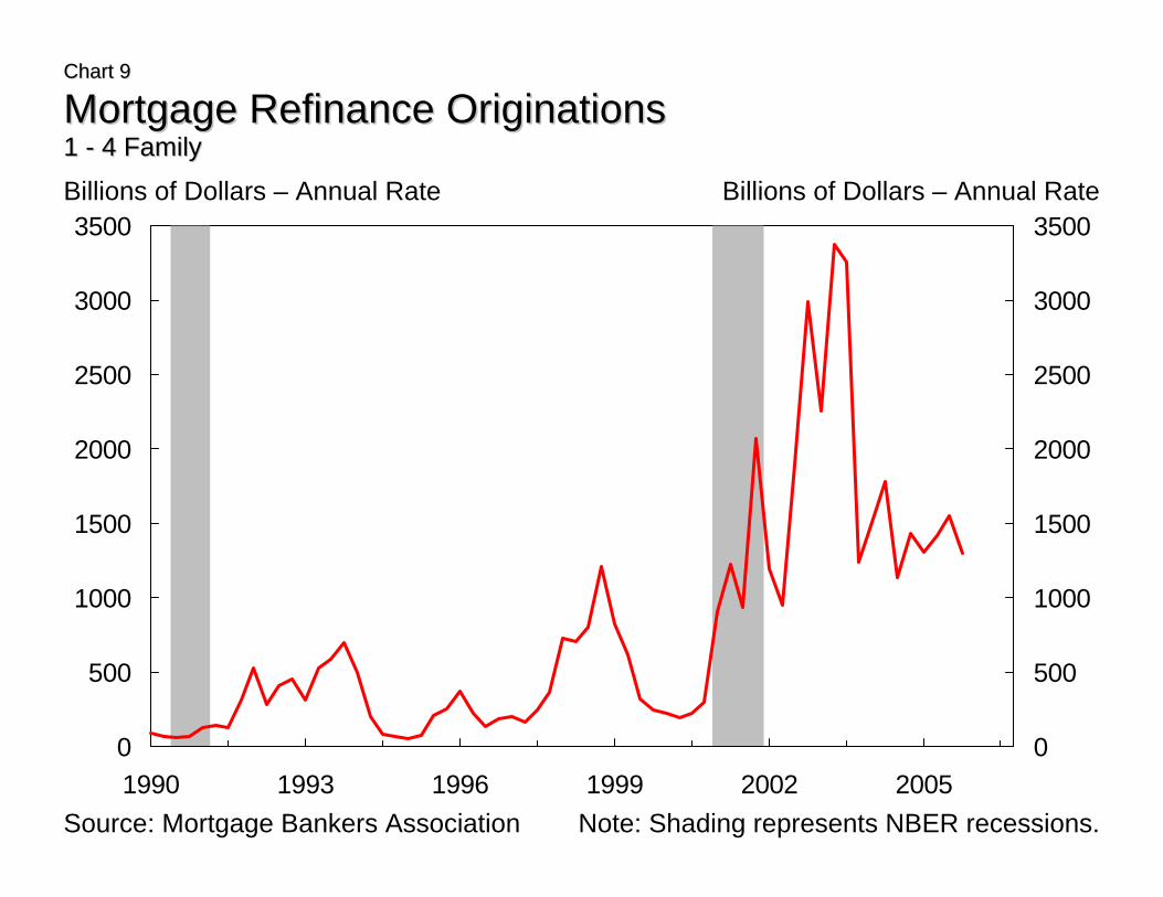
Along with the large increases in home values in recent years has come an unprecedented wave of

mortgage refinancings, encouraged by both home price increases and low interest rates. While refinancings

have ebbed from their extraordinary pace of 2003, the gross value of mortgage refinance originations was

nearly $1.3 trillion in 2005 (Chart 9). While the bulk of these funds probably were used to liquidate

existing prior mortgages, there typically are considerable funds remaining for other purposes. One measure

of such funds is based on work by Greenspan and Kennedy (2005), which includes explicit equity

withdrawal through refinancings along with implicit withdrawals through mortgage payments.20 Based on

their methodology, mortgage equity withdrawal by households was between $700 and $900 billion in 2005

(Chart 10).21 In principle, these funds are available to finance consumer spending.

As suggested above, we view the increase in refinancings as connected to the secular trend of

increased availability of credit to U.S. households, with the favorable developments in home prices and

interest rates fueling the recent upsurge. It could well be the case that this increased availability of credit

has provided some support to consumption growth in recent years, though we do not think the dollar

amount of equity extraction is a valid measure of availability.

A vexatious issue is the assessment of the spending implications of the funds extracted from home

equity. At one extreme, equity extractions can be viewed as financial decisions entirely independent of

basic spending and saving decisions, a view consistent with the standard life-cycle/permanent-income

19 Also, Iacoviello (2004) notes that his results are only applicable to anticipated changes in home prices. If one believes that the recent increases have been largely unanticipated his results are not applicable. 20 Specifically, they compute the amount of borrowing to finance home purchases at average loan-to-value ratios and then take the difference between this amount and the change in mortgage debt outstanding to determine gross equity extraction. 21 The smaller net number removes mortgage transactions fees, points, and taxes from gross mortgage equity withdrawal.

17

model. In the aggregate, equity extraction redirects interest expenses and income across households

(McConnell, Peach, and al-Hashimi (2003)); consequently, the net effect on consumption would be quite

small. At the other extreme, the funds raised from home equity extraction could be viewed as equivalent to

straight household income and thus have a major effect on spending. Under this latter view, if home equity

extractions are reduced because of higher interest rates and/or a correction in home prices, spending growth

would then be at risk.

The available empirical results are subject to these varying interpretations. A 2002 study of the

use of funds from mortgage refinancings (Canner, Dynan, and Passmore (2002)) found that perhaps $18

billion in spending in 2001—16 percent of the dollar volume of home equity extracted through

refinancings—was financed through this means (the balance of the equity extracted through refinancings

was used for home repairs, alterations, and improvements, as well as to restructure other components of

household balance sheets). The gross dollar volume of refinancings in 2005 was comparable to that in

2001, so one view is that equity extraction recently has been a relatively minor contributor to consumer

spending. More extreme would be the view that most of this additional spending still would have occurred

even without the refinancings, which would imply that the refinancing has little contribution. At another

extreme, if we apply the 16 percent ratio to 2005 estimate of home equity extraction, then between $110

billion and $150 billion of consumer spending was financed through this means last year.22

However, these larger values probably would not be accurate estimates of the amount of spending

at risk from a weakening in the housing market. First, it is not clear if the 2001 ratio would be applicable

for 2005. Secondly, it would be rather extreme to project the outright disappearance of the refinance

market in any circumstance.23 More substantively, the increased ease and lower cost of mortgage

refinancings, along with the tax-exempt status of mortgage interest payments, suggests that refinancings

likely have displaced many other means of raising funds to finance spending. Equity extraction,

particularly through refinancings, rather than an independent source of spending, may essentially be a

primary mechanism through which spending arising from capital gains on homes is financed.

22 The lower figure refers to the “net” mortgage equity withdrawal estimate; the higher figure refers to the “gross” value. 23 As noted above, Hurst and Stafford (2004) found that some households would refinance after an unemployment shock even if the refinancing was not financially advantageous.

18

One piece of evidence that many analysts have pointed to in arguing that, contrary to our analysis,

housing wealth gains and home equity withdrawal have had large spillovers to consumer spending (and

thus a housing slowdown puts much consumption at risk) is the recent decline in the personal saving rate.

In Appendix 2, we address this issue and find that an alternative explanation, the shift of private income

toward undistributed corporate profits, can explain much of the recent decline in the saving rate.

Adding up the Risks

The recent data suggest that some aspects of housing activity have fallen from their peak levels.

Residential investment has consistently contributed nearly one-half percentage point to overall GDP growth

over the past few years. A removal of this contribution and a turn to contraction would have a noticeable

impact on aggregate growth, unless activity accelerated in some other sector. Nonetheless, housing

weakness would need to spread to other sectors to have the substantial effect on aggregate activity that is

incorporated in outlooks where housing is the current economic linchpin. Clearly, the sector of concern in

that regard would be consumer spending.

Our read of the evidence on the linkages is that there is some risk that a period of sustained

weakness in housing activity and values would have a noticeable impact on the growth of consumer

spending. One linkage is direct: certain types of spending have clear ties to home sales and purchases.

These spending categories have grown rapidly in recent years, and a contraction in housing could quite

likely lead to some slowdown in their growth. Nonetheless, the aggregate amount of spending in these

areas, and their contribution to overall GDP growth, has been quite limited.

The more substantive risk arises from the possibility that slower growth or declines in housing

prices would lead to reduced growth in consumer spending. The primary mechanism by which this could

happen is a traditional wealth effect: the view that there is a substantive connection between changes in the

value of household wealth, including those generated by changes in housing values, and changes in

consumer spending. Another possible mechanism is the equity extraction effect—the view that high values

of home equity facilitate household borrowing and spending. This mechanism could be one avenue

through which the wealth effect operates, or it could be a separate effect enabling households to consume at

levels not previously achievable. The risk then is that the effect of a slowdown in the growth of home

19

prices would be two-fold: added to the direct wealth effect would be a further mechanism by which

households no longer able to borrow against home equity would cut back spending.

These risks look real, but their size is quite problematic. Our review of the evidence is that 0.025

to 0.05 may be a plausible range of the propensity to consume from permanent changes in home values.

Recent years have seen capital gains on homes averaging close to $2 trillion a year: assuming that the

propensity to consume is in the above-cited range, roughly $50 to $100 billion a year was added to

consumer spending through housing wealth effects (some of that spending has likely been in the form of

expenditures directly tied to housing transactions). It could be that this spending effect estimate is high,

since it is possible that households regard much of the recent unusually strong increase in home values as

transitory. Nevertheless, taking these estimates at face value, it would be the case that a cessation of this

support would have a substantive impact on the growth of consumer spending.

In addition, we find no striking evidence that there have been large recent changes in households’

ability to use home equity as a means to overcome borrowing constraints or as a potential source of

precautionary savings. The huge amount of funds realized through equity extractions in recent years

probably reflects the exploitation of opportunities to recalibrate household balance sheets, rather than a sign

of a behavioral shift in spending associated with a changed financial environment. In any event, even with

the large volumes of equity extraction the aggregate ratio of equity to home values has remained well above

50 percent. However, because there is little no evidence bearing on the recent disposition of the large

amount of funds raised through equity extraction, it is possible that a good deal of spending could have

occurred due to the availability of this means of finance.

Of course, there is always the potential for an even larger slowdown of consumer spending growth

if household wealth (including home values) falters. Our analysis suggests that the significant risks would

stem from changes in underlying perceptions of the longer-term growth prospects of the economy, which

have the potential to hamper both spending and valuations. Fluctuations in asset values stemming from

developments isolated to the housing market appear to have less potential to influence spending, unless

they are so large as to imply major changes in the availability of home equity as a means of finance.

20

Appendix 1. Stability of Consumption Equations

Our interpretation of the evidence concerning the effects of housing wealth on consumer spending

is predicated in part on two premises. First, the propensity to consume out of housing wealth does not

differ drastically from that out of nonhousing wealth. Second, the propensity to consume out of wealth

depends upon household views of the “permanence” of wealth changes and thus is not stable over time.

We examine these premises briefly within an Euler equation model similar to that used in

Campbell and Mankiw (1989), augmented to included growth in housing and nonhousing wealth.

Specifically, we estimate the following regression.

(A1) tht

ntttt wwyrc εααααα +∆+∆+∆++=∆ −−− 14131210

In this regression, ∆c is the growth rate of real per capita consumption (defined as the chained aggregate of

nondurable and services consumption), r is a real three-month T-bill rate, ∆y is the growth rate of real per

capita labor income (defined similarly as in Lettau and Ludvigson (2004)), and ∆wn and ∆wh are the growth

rates of real per capita nonhousing and housing wealth respectively.

Once we estimate the model, we examine our premises using two statistical tests. First, we test

whether the coefficients on nonhousing and housing wealth (α3 and α4, respectively) are equal. Second, we

test for the stability of model using a statistic developed in Hansen (1992), which allows for the possibility

of more general forms of instability than do structural break tests such as Chow tests. Evidence of

instability would be consistent with our premise that the propensity to consume out of wealth is not stable

over time.

The results of estimating equation (A1) are presented in the first column of Appendix Table A1.24

The coefficient estimates on the short-term interest rate and income growth are in rough accord with the

results from Campbell and Mankiw (1989). The coefficient on the interest rate is small and statistically

insignificant. The coefficient on income growth is positive and statistically significant: it is somewhat

smaller than the Campbell and Mankiw estimates, but it still signifies that realized income growth has a

substantial effect on consumption growth.

The coefficients on nonhousing and housing wealth are both positive, although only the one on

nonhousing wealth is statistically significant. Even so, the null hypothesis that the coefficients on the two

21

wealth variables are equal cannot be rejected: the p-value of the statistic is over 0.35. In fact, when

estimating equation (A1) by replacing the growth of housing and nonhousing wealth with the growth of

total wealth, the coefficient on total wealth is highly statistically significant and the fit of the regression is

similar, as seen in the second column of Table A1. These results imply that when estimating the propensity

to consume from a long sample, the propensity out of housing wealth does not differ drastically from that

out of nonhousing wealth.25

Turning to the stability of the model in equation (A1), the stability test statistics indicate that the

regression is not stable both in the case where the wealth variables are entered separately (column 1) and in

the case where they entered in a single total wealth variable (column 2); the test statistic rejects the null of

stability easily at the one percent significance level. This implies that estimating propensities to consume

from long-sample regressions such as this is fraught with hazard. Examining some additional information

from stability test statistics (not shown in Table A1 to conserve space) indicates much of the instability

results from a nonconstant variance of the error term in the regression. This observation in turn implies that

the coefficients on the variables in the regression probably are not stable. In particular, it is unlikely that

the estimates of the propensity to consume from models like the one presented here are stable, which is

consistent with our second premise.

24 The sample period in our estimation is 1960Q1-2006Q1. 25 However, it is possible that the propensities may differ over shorter samples if they fluctuate over time.

22

Appendix 2. Housing and the Saving Rate

Our view of the evidence is that housing gains (along with the recovery in the stock market since

2003) have likely made some significant contribution to recent growth in consumer spending but it may be

an overstatement to claim that housing has been as a predominant determinant. Instead, the increase in

home values may have been to a substantive degree related to forces such as productivity improvement

(and with it, long-term income prospects) that are major drivers of spending over the longer term.

One counter to this argument is the decline in the personal saving rate in 2004 and 2005. The

personal saving rate was negative in 2005 according to currently available data. One conclusion that many

have drawn is that the sharp recent increases in housing wealth have increased spending relative to income

and driven down the saving rate, or in popular terms, consumers have saved through their homes.

While this contention is a superficially plausible, a closer examination suggests a more complex

story. Specifically, consumer spending has increased relative to personal disposable income, driving down

personal saving. However, there were also very large increases in the amount of undistributed corporate

profits in 2004 and 2005—the one component of private sector income not credited to household income in

the national accounts and saving data. If the household income and saving data are both augmented to

include undistributed profits the 2004-05 drop in the saving rate disappears (Chart A1). Therefore, the

recent decline in the personal saving rate, rather than reflecting a step-up in consumption, may be in large

part an artifact of a shift in private sector income away from households and toward corporate undistributed

earnings. It is certainly possible to assert, as has been maintained at times in the past, that the spending

decisions of shareholders are relatively insensitive to the division of corporate income between dividends

and undistributed profits (Feldstein (1973), Steindel (1977, 1981)).

23

References Ando, Albert, and Franco Modigliani. 1963. “The ‘Life Cycle’ Hypothesis of Saving: Aggregate

Implications and Tests.” American Economic Review, vol. 53, pp. 55-84. Aoki, Kosuke, James Proudman, and Jan Vliege. 2004. “House Prices, Consumption, and Monetary

Policy: A Financial Accelerator Approach.” Journal of Financial Intermediation, vol. 13, pp. 414-435.

Baker, Dean. 2006. “The Menace of an Unchecked Housing Bubble.” The Economists’ Voice, Vol. 3, No.

4, Article 1. <http://www.bepress.com/ev/vol3/iss4/art1> Belsky, Eric, and Joel Prakken. 2004. “Housing Wealth Effects: Housing’s Impact on Wealth

Accumulation, Wealth Distribution and Consumer Spending.” Harvard University, Joint Center for Housing Studies, W04-13.

Benjamin, John D., Peter Chinloy, and G. Donald Jud. 2004. “Real Estate Versus Financial Wealth in

Consumption.” Journal of Real Estate Finance and Economics, vol. 29, pp. 341-354. Bernanke, Ben S., Mark Gertler, and Simon Gilchrist. 1999. “The Financial Accelerator in a Quantitative

Business Cycle Framework.” In John B. Taylor and Michael Woodford (eds.), Handbook of Macroeconomics, Vol. 1C. Amsterdam: Elsevier, North Holland, pp. 1341-93.

Bostic, Raphael, Stuart Gabriel, and Gary Painter. 2005. “Housing Wealth, Financial Wealth, and

Consumption: New Evidence from Micro Data.” Lusk Center for Real Estate, University of Southern California.

Bucks, Brian K., Arthur B. Kennickell, and Kevin B. Moore. 2006. “Recent Changes in U.S.

Family Finances: Evidence from the 2001 and 2004 Survey of Consumer Finances.” Federal Reserve Bulletin, vol. 92, <www.federalreserve.gov/pubs/bulletin/2006/financesurvey.pdf>.

Campbell, John Y., and N. Gregory Mankiw. 1989. “Consumption, Income, and Interest Rates:

Reinterpreting the Time Series Evidence.” In Olivier J. Blanchard and Stanley Fischer (eds.), NBER Macroeconomics Annual: 1989. Cambridge, MA: MIT Press, pp. 185-216.

Canner, Glenn, Karen Dynan, and Wayne Passmore. 2002. “Mortgage Refinancing in 2001 and Early

2002.” Federal Reserve Bulletin, vol. 88, pp. 470-481. Carroll, Christopher D. 1997. “Buffer-Stock Saving and the Life Cycle/Permanent Income Hypothesis.”

Quarterly Journal of Economics, vol. 112, pp. 1-55. Davis, Morris A., and Michael G. Palumbo. 2001. “A Primer on the Economics and Time Series

Econometrics of Wealth Effects. Federal Reserve Board Finance and Economics Discussion Paper No. 2001-09.

Deaton, Angus. 1991. “Saving and Liquidity Constraints.” Econometrica, vol. 59, pp. 1221-48. Feldstein, Martin S. 1973. “Tax Incentives, Corporate Saving, and Capital Accumulation in the United

States.” Journal of Public Economics, vol. 2, pp. 159-171. Friedman, Milton. 1957. A Theory of the Consumption Function. Princeton. Greenspan, Alan and James Kennedy. 2005. “Estimates of Home Mortgage Originations, Repayments,

and Debt on One-to-Four Family Residences.” Federal Reserve Board Finance and Economics Discussion Series 2005-41.

24

Hall, Robert. 1978. “Stochastic Implications of the Life Cycle-Permanent Income Hypothesis: Theory and Evidence.” Journal of Political Economy, vol. 86, pp. 971-987.

Hansen, Bruce. 1992. “Testing for Parameter Instability in Linear Models.” Journal of Policy Modeling,

vol. 14, pp. 517-533. Himmelberg, Charles, Christopher Mayer, and Todd Sinai. 2005. “Assessing High House Prices:

Bubbles, Fundamentals and Misperceptions.” Journal of Economic Perspectives, vol., 19, no. 4, pp. 67-92.

Hurst, Erik, and Frank Stafford. 2004. “Home is Where the Equity is: Mortgage Refinancing and

Household Consumption.” Journal of Money, Credit, and Banking, vol. 36, pp. 985-1014. Iacoviello, Matteo. 2004. “Consumption, House Prices, and Collateral Constraints: A Structural

Econometric Analysis.” Journal of Housing Economics, vol. 13, pp. 304-320. ________. 2005. “House Prices, Borrowing Constraints, and Monetary Policy in the Business Cycle.”

American Economic Review, Vol. 95, pp. 739-64. Juster, F. Thomas, Joseph P. Lupton, James P. Smith, and Frank Stafford (2006). “The Decline in

Household Saving and the Wealth Effect.” Review of Economics and Statistics, vol. 87, no. 4, pp. 20-27.

Lehnert, Andreas. 2004. “Housing, Consumption, and Credit Constraints.” Federal Reserve Board

Finance and Economics Discussion Series 2004-63 (September). Lettau, Martin, and Sydney Ludvigson. 2003. “Consumption, Aggregate Wealth, and Stock Returns.”

Journal of Finance, vol. 56, pp. 815-49. ____. 2004. “Understanding Trend and Cycle in Asset Values: Reevaluating the Wealth Effect on

Consumption,” American Economic Review, vol. 94, pp. 276-299. Ludvigson, Sydney. 2003. “Analyzing the Linkage Between Consumption and Wealth.” Presented to the

Federal Reserve Bank of Philadelphia Policy Forum, November 14, 2003. <http://www.phil.frb.org/econ/conf/forum2003/Ludvigson_final.pdf>.

____, and Charles Steindel. 1999. “How Important is the Stock Market Effect on Consumption?” Federal

Reserve Bank of New York Economic Policy Review, vol. 5, no. 2, pp. 29-51. Lustig, Hanno, and Stijn van Nieuwerburg. 2005. “Housing Collateral, Consumption Insurance and Risk

Premia: An Empirical Perspective.” Journal of Finance, vol. 60, pp. 1167-1219. McCarthy, Jonathan. 1995. “Imperfect Insurance and Differing Propensities to Consume Across

Households.” Journal of Monetary Economics, vol. 36, pp. 301-327. _____, , and Richard W. Peach. 2002. “Monetary Policy Transmission to Residential Investment.”

Federal Reserve Bank of New York Economic Policy Review, Vol. 8, No. 1, pp. 139-58. ______. 2004. “Are Home Prices the Next ‘Bubble’?” Federal Reserve Bank of New York Economic

Policy Review, Vol. 10, No. 3, pp. 1-17. McConnell, Margaret, Richard Peach, and Alex Al-Hashimi. 2003. “After the Refinancing Boom: Will

Consumers Scale Back Their Spending?” Federal Reserve Bank of New York Current Issues in Economics and Finance, vol. 9, no. 12.

25

Shiller, Robert J. 2006. “Long-Term Perspectives on the Current Boom in Home Prices.” The Economists' Voice, Vol. 3, No. 4, Article 4. <http://www.bepress.com/ev/vol3/iss4/art4>.

Steindel, Charles. 1977. Personal Consumption, Property Income, and Corporate Saving. Ph. D. thesis,

Department of Economics, Massachusetts Institute of Technology. ____. 1981. “The Determinants of Private Saving.” In Public Policy and Capital Formation (Jared

Enzler, William Conrad, and Lewis Johnson, eds.), Board of Governors of the Federal Reserve System.

____. Forthcoming. “The Consumption Wealth Effect.” In Critical Perspectives on Recent

Developments in Macroeconomics (Per Gunnar Berglund and Leanne J. Ussher, eds), Routledge. Tracy, Joseph, Henry Schneider, and Sewin Chan. 1999. “Are Stocks Overtaking Real Estate in

Household Portfolios?” Federal Reserve Bank of New York Current Issues in Economics and Finance, vol. 5, no. 5.

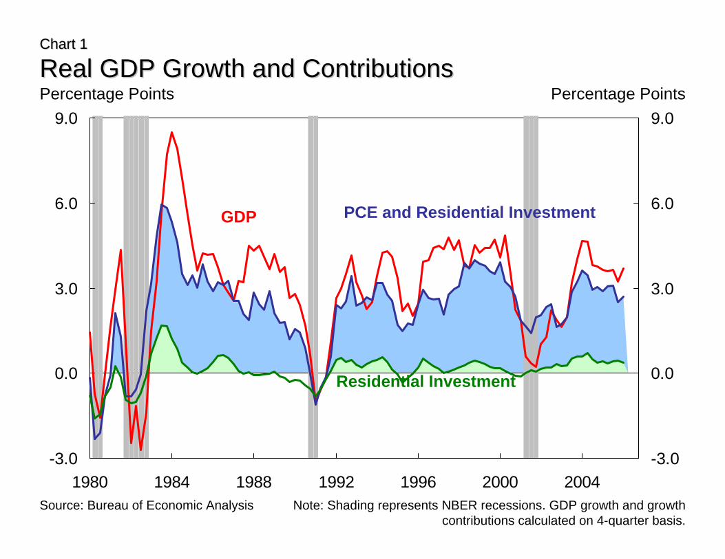
Chart 1Chart 1

Real GDP Growth and ContributionsReal GDP Growth and Contributions

-3.0

0.0

3.0

6.0

9.0

1980 1984 1988 1992 1996 2000 2004-3.0

0.0

3.0

6.0

9.0Percentage Points Percentage Points

GDP PCE and Residential Investment

Residential Investment

Source: Bureau of Economic Analysis Note: Shading represents NBER recessions. GDP growth and growth contributions calculated on 4-quarter basis.

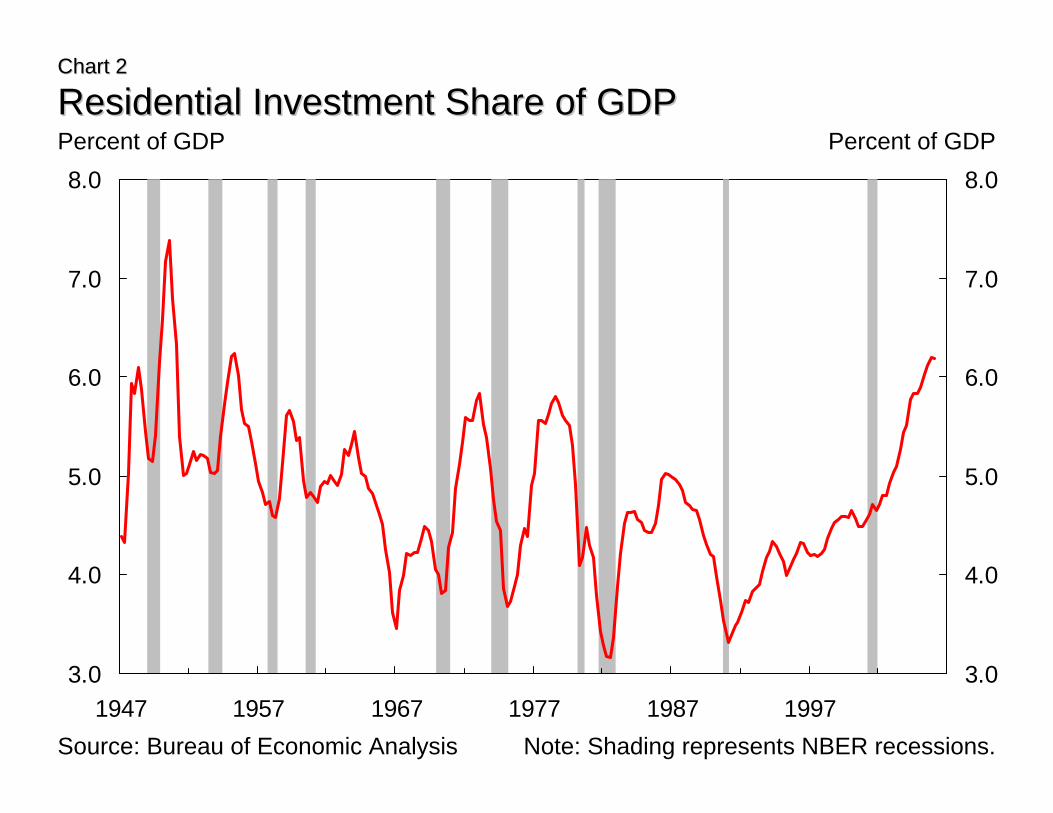
Chart 2Chart 2

Residential Investment Share of GDPResidential Investment Share of GDPPercent of GDP Percent of GDP

Source: Bureau of Economic Analysis Note: Shading represents NBER recessions.

3.0

4.0

5.0

6.0

7.0

8.0

1947 1957 1967 1977 1987 19973.0

4.0

5.0

6.0

7.0

8.0

-5

0

5

10

15

1976 1980 1984 1988 1992 1996 2000 2004-5

0

5

10

15

Chart 3Chart 3

Home Price AppreciationHome Price Appreciation

Real Appreciation

OFHEO IndexNominal

Appreciation

16% 70%14%

% Change - Year to Year% Change - Year to Year

Source: Office of Federal Housing Enterprise Oversight and Bureau of Economic Analysis.

Note: Shading represents NBER recessions. Numbers in shaded region represent cumulative real appreciation during that episode

(3.8%)(2.3%) (5.1%)

Total: $32.7 Trillion

2000

2005

Other$17.1 Trillion

Other$22.2 Trillion

Other$29.8 Trillion

Stock$15.3 Trillion

Real Estate$11.4 Trillion

Real Estate$8.0 Trillion

Real Estate$19.9 Trillion

Stock$7.6 Trillion

Stock$14.7 Trillion

Chart 4Chart 4

AssetsAssets 1995

Total: $48.9 Trillion Total: $64.4 Trillion

Source: Flow of Funds, Federal Reserve Board

Total: $27.7 Trillion

2000

2005

Other$15.4 Trillion

Other$19.6 Trillion

Other$26.5 Trillion

Stock$15.3 Trillion

Real Estate$6.6Trillion

Real Estate$4.7 Trillion

Real Estate$11.2 Trillion

Stock$7.6 Trillion

Stock$14.7 Trillion

Chart 5Chart 5

Net WorthNet Worth1995

Total: $41.5 Trillion Total: $52.4 Trillion

Source: Flow of Funds, Federal Reserve Board

4

5

6

7

1980 1984 1988 1992 1996 2000 20044

5

6

7Ratio Ratio

0

1

2

3

4

1980 1985 1990 1995 2000 20050

1

2

3

4

Total

Stock and Real Estate

Real Estate

Source: Flow of Funds, Federal Reserve Board, and Bureau of Economic Analysis Note: Shading represents NBER recessions.

Chart 6Chart 6

Net Worth Relative to Disposable Personal Income Net Worth Relative to Disposable Personal Income

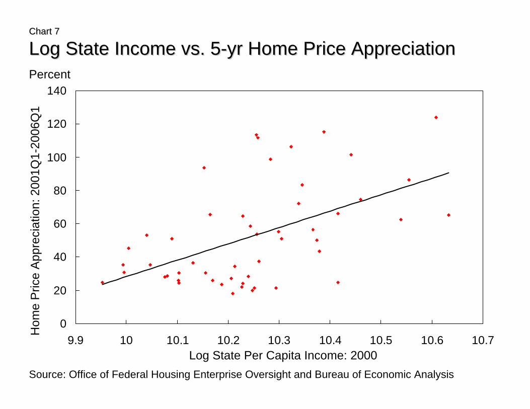
Chart 7Chart 7

Log State Income vs. 5Log State Income vs. 5--yr Home Price Appreciationyr Home Price Appreciation

0

20

40

60

80

100

120

140

9.9 10 10.1 10.2 10.3 10.4 10.5 10.6 10.7

Percent

Log State Per Capita Income: 2000Source: Office of Federal Housing Enterprise Oversight and Bureau of Economic Analysis

Hom

e P

rice

App

reci

atio

n: 2

001Q

1-20

06Q

1

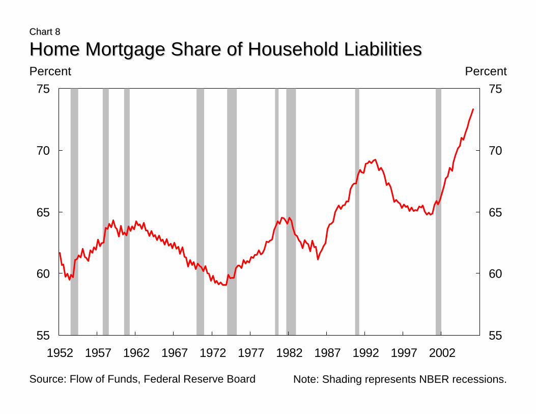
Chart 8Chart 8

Home Mortgage Share of Household LiabilitiesHome Mortgage Share of Household Liabilities

55

60

65

70

75

1952 1957 1962 1967 1972 1977 1982 1987 1992 1997 200255

60

65

70

75Percent Percent

Source: Flow of Funds, Federal Reserve Board Note: Shading represents NBER recessions.

0

500

1000

1500

2000

2500

3000

3500

1990 1993 1996 1999 2002 20050

500

1000

1500

2000

2500

3000

3500

Chart 9Chart 9

Mortgage Refinance OriginationsMortgage Refinance Originations1 1 -- 4 Family4 Family

Billions of Dollars – Annual Rate Billions of Dollars – Annual Rate

Source: Mortgage Bankers Association Note: Shading represents NBER recessions.

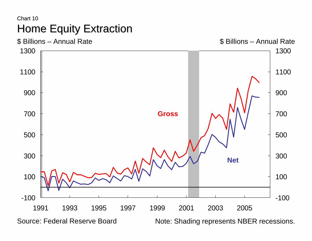
Chart 10Chart 10

Home Equity ExtractionHome Equity Extraction

-100

100

300

500

700

900

1100

1300

1991 1993 1995 1997 1999 2001 2003 2005-100

100

300

500

700

900

1100

1300$ Billions – Annual Rate $ Billions – Annual Rate

Gross

Net

Source: Federal Reserve Board Note: Shading represents NBER recessions.

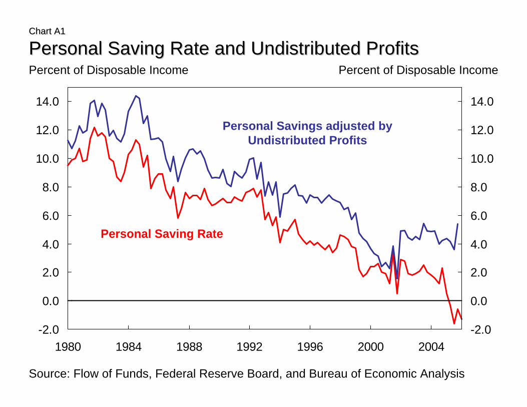
Chart A1Chart A1

Personal Saving Rate and Undistributed ProfitsPersonal Saving Rate and Undistributed Profits

-2.0

0.0

2.0

4.0

6.0

8.0

10.0

12.0

14.0

1980 1984 1988 1992 1996 2000 2004-2.0

0.0

2.0

4.0

6.0

8.0

10.0

12.0

14.0

Percent of Disposable Income Percent of Disposable Income

Personal Saving Rate

Personal Savings adjusted by Undistributed Profits

Source: Flow of Funds, Federal Reserve Board, and Bureau of Economic Analysis

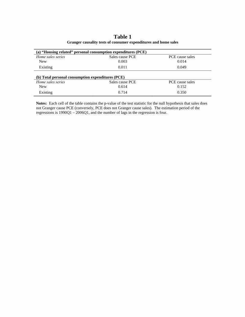
Table 1

Granger causality tests of consumer expenditures and home sales (a) “Housing related” personal consumption expenditures (PCE) Home sales series Sales cause PCE PCE cause sales New 0.003 0.014 Existing 0.011 0.049

(b) Total personal consumption expenditures (PCE) Home sales series Sales cause PCE PCE cause sales New 0.614 0.152 Existing 0.714 0.350 Notes: Each cell of the table contains the p-value of the test statistic for the null hypothesis that sales does not Granger cause PCE (conversely, PCE does not Granger cause sales). The estimation period of the regressions is 1990Q1 – 2006Q1, and the number of lags in the regression is four.

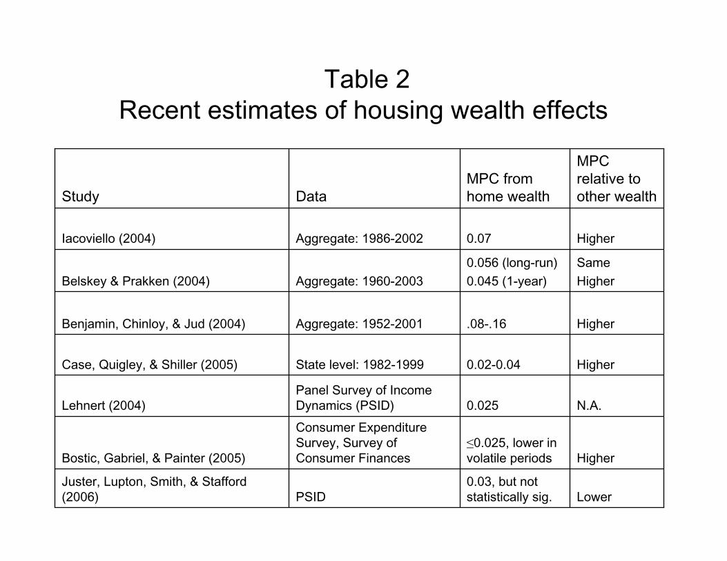
Table 2Recent estimates of housing wealth effects

Higher.08-.16Aggregate: 1952-2001Benjamin, Chinloy, & Jud (2004)

Lower0.03, but not statistically sig.PSID

Juster, Lupton, Smith, & Stafford (2006)

Higher≤0.025, lower in volatile periods

Consumer Expenditure Survey, Survey of Consumer FinancesBostic, Gabriel, & Painter (2005)

N.A.0.025Panel Survey of Income Dynamics (PSID)Lehnert (2004)

Higher0.02-0.04State level: 1982-1999Case, Quigley, & Shiller (2005)

SameHigher

0.056 (long-run)0.045 (1-year)Aggregate: 1960-2003Belskey & Prakken (2004)

Higher0.07Aggregate: 1986-2002Iacoviello (2004)

MPC relative to other wealth

MPC from home wealthDataStudy

Appendix Table A1 Estimates of equation (A1)

Variable (1) (2) Constant 1.803***

(0.229) 1.824*** (0.225)

Interest rate -0.088 (0.065)

-0.090 (0.065)

Income growth 0.132** (0.053)

0.138*** (0.048)

Nonhousing wealth growth 0.048*** (0.011)

Housing wealth growth 0.023 (0.022)

Total wealth growth 0.060*** (0.013)

R-bar squared 0.169 0.171 Stability test statistic 2.656*** 2.336*** Equality of nonhousing and housing coefficients: Chi-squared (1) statistic: (p-value)

0.871

(0.351)

Notes: The sample period is 1960Q1-2006Q1. Standard errors are shown in parentheses below the parameter estimate. *** denotes statistical significance at the 1% level; ** denotes statistical significance at the 5% level. The distribution for the stability test statistic comes from Hansen (1992): in column (1), the 1% critical value is 2.12; in column (2), the 1% critical value is 1.88.