Housing and Monetary Policy in the Business Cycle: What do

Housing Rents have to say?∗

Joao B. Duarte† Daniel A. Dias‡

January 2016

Abstract

In this paper we unveil a feedback loop between monetary policy, housing tenure choice

(own vs rent) and measured inflation and quantify its consequences. This feedback loop is ex-

plained in three parts: i) Housing rents respond positively to contractionary monetary policy

shocks; ii) This effect of interest rates on housing rents gives rise to an important and system-

atic inflation mismeasurement problem because, directly and indirectly, housing rents weigh

approximately 30% in the CPI and 13% in the PCE; iii) When interest rates are set according to a

Taylor rule, the systematic mismeasurement of inflation gives rise to a feedback loop by which

the monetary authority keeps setting interest rates too high (low) because inflation is appar-

ently too high (low). To rationalize i) and quantify the importance of iii) we propose a standard

New Keynesian model augmented with an endogenous housing tenure choice mechanism. Us-

ing a calibrated version of the model, we do a counterfactual exercise and estimate that, when

the monetary authority targets the implied consumer price index net of housing rents instead

of the implied consumer price index, the loss function of monetary policy is 14.5% lower and

the welfare in terms of consumption equivalent variation is 0.9% higher. Finally, analysing the

same alternative scenario for the 1983-2006 US experience, we find that the standard deviation

of housing prices and nominal inflation would have been 24.8% and 19.9% lower, respectively.

JEL classification codes: E31, E43, R21.

Key Words: Housing Rents, Housing Tenure Choice, Monetary Policy, CPI, DSGE, SVAR, FAVAR,

Business Cycle.

∗The authors thank, without implicating, Chris Sims, Harald Uhlig, Stephen Parente, Dan Bernhardt, Minchul Shin,Geoffrey Hewings, Mark Wright, Alejandro Justiniano, Leonardo Melosi and various participants at the macro readinggroup at UIUC and REAL seminar series for helpful suggestions and discussions. This research was supported by thePaul Boltz Fellowship and the UIUC campus research board with an Arnold O. Beckman Research Award. The views inthis paper are solely the responsibility of the authors and should not be interpreted as reflecting the views of the Board ofGovernors of the Federal Reserve System or of any other person associated with the Federal Reserve System. All errorsare our own.

†Department of Economics, University of Illinois at Urbana-Champaign. Email: aurelio2@illinois.edu.‡Board of Governors of the Federal Reserve System and CEMAPRE. Email: daniel.dias@frb.gov.

1

1 Introduction

Since the 2007/2008 financial crisis the efforts to better understand the links between housing

and the macroeconomy have been enormous and a large amount of new research has been produced

since then. The bulk of the literature on housing and the macroeconomy has focused almost entirely

on the role of house prices on different economic outcomes such as output, consumption or financial

stability. Interestingly, housing rents, which are obviously related to house prices, have been, to the

best of our knowledge, completely overlooked.

In this paper, we fill this gap in the literature and unveil and quantify the importance of a new

link between monetary policy and the housing market that operates through the effect of monetary

policy on housing rents and vice-versa. Before explaining this channel of monetary policy, we must

first introduce a new stylized fact regarding the effect of monetary policy on housing rents, and

highlight the importance of housing rents in the most commonly used measures of inflation, the

consumer price index (CPI) and the personal consumption expenditures (PCE) price index.

New stylized fact: we show housing rents respond positively to contractionary monetary pol-

icy shocks using SVAR and FAVAR models and structural shock identification techniques on US

data. Specifically, we find that when the federal funds rate is raised by 25 basis points, housing

rents increase by 1.22% after five years. Our empirical findings are obtained in the context of em-

pirical models that also include house prices, which were already known to respond negatively to

contractionary monetary policy shocks (Iacoviello (2005), Del Negro and Otrok (2007)). Hence, it is

surprising that housing rents increase when income, other sale prices and housing prices fall after

that same unexpected increase in interest rates.

One possible explanation for these two apparently conflicting results, house prices declining

while house rents increase in response to a contractionary monetary policy shock, is the effect that

monetary policy may have on housing tenure decisions (own vs. rent). If for some reason the

prices of houses and rents do not adjust quickly enough to its new long-run nominal level after

a contractionary monetary policy shock, the relative costs of owning vs. renting will change, and

this will lead to some people switching from one type of tenure to the other. In support of this

interpretation, we show that after a contractionary monetary policy shock rental vacancy rates,

homeownership rates and housing starts decline while homeowner vacancy rates increase.

Importance of housing rents in the CPI or PCE: since the adoption of the owner equivalent

rent (OER) estimate in 1983 as a measure of shelter costs faced by homeowners that live in their

2

own house, that the direct and indirect weight of housing rents in the CPI has been over 20%,

and currently surpassing 30%. In the case of PCE, which uses the same information coming from

the housing rental market, the current weight of shelter in the overall index is lower than in the

case of CPI and is just slightly above 13% of the total index. 1 The reason why housing rents

have such a large weight on total CPI and total PCE is because in the estimation of the OER the

Bureau of Labor Statistics (BLS) uses information from the housing rental market to impute rental

prices to houses that are owner-occupied (see BLS CPI methodology (2009) for more details on this

procedure). Reflective of this is the fact that the correlation between the year-on-year growth rates

of housing rent and OER is around 0.85. Hence, the shelter component of CPI and PCE is almost

entirely driven by the housing rental market.

The new channel of monetary policy that we claim to unveil is as follows: when the monetary

authority increases (decreases) interest rates, real housing rents increase (decrease). This creates a

measurement issue in tracking underlying nominal inflation and leads to a downward (upward)

biased estimate of inflation when CPI or PCE are used. Because directly and indirectly, housing

rents have a fairly large weight on CPI and PCE, this bias may be sufficiently large and lead the

monetary policy authority to keep setting interest rates too high (low) in its attempt to achieve a

certain inflation target. This feedback can add unnecessary variation to the underlying inflation

rate and housing prices, and generate large welfare costs and losses to a monetary policy whose

objective is to minimize inflation and output gap variance.

To formalize and quantify the importance of this mechanism we add an endogenous housing

tenure choice mechanism and heterogeneous agents to a standard New Keynesian model (Clarida,

Gali and Gertler (1999)). By including housing rents, we can introduce a theoretical CPI in the model

that is constructed based on a weighted basked of housing rents and composite consumption good.

We calibrate the model to match key features of the U.S. economy assuming the monetary authority

reacts to CPI, and show that it fits remarkably well some of the data moments that are not targeted

by the calibration exercise. Moreover, with our model, we are able to endogenously generate a price

puzzle without having to assume that there is a cost channel of monetary policy. 2

With the calibrated model we do a counterfactual exercise where we compare both aggregates

1If we excluded the food and energy components from CPI and PCE, that is, if our reference was not total CPI or totalPCE but core CPI and core PCE, the current weights of shelter in core CPI would be over 40% and over 17% in the caseof core PCE.

2In a companion paper, Dias and Duarte (2015), we explore this result further, and show that to a large extent the pricepuzzle can be explained by the response of shelter to monetary shocks. In addition, we also show that inflation is muchless persistent than what analyses based on overall CPI or PCE suggest.

3

and price dynamics of the calibrated model, the benchmark case, whereby we assume the interest

rate Taylor rule takes CPI as input, to an alternative setting where the Taylor rule takes a rents-free

consumer price index as input. Our counterfactual exercises reveal that: 1) targeting a measure

of inflation that excludes housing rents leads to a 0.9% welfare gain in consumption equivalent

variation and to a 14.5% fall in the loss function of monetary policy whose objective is to minimize

inflation and output gap variance; 2) we estimate that this mechanism can explain 37.5% of the

increase in house prices above trend3 that occurred between 2002 and 2007; 3) under the alternative

scenario, we find that the standard deviation of housing prices and nominal inflation would have

been 24.8% and 19.9% lower for the 1984-2006 US experience, respectively.

In this paper, we do not argue for the exclusion of housing rents from the CPI in every cir-

cumstance. Housing rents are an important item on measuring households cost of living since

households spend around 30% of their income with shelter, and hence should be part of the con-

sumer price index. In general, price indexes trends capture well the evolution of the nominal state

of the economy. However, when relative prices of some specific goods change suddenly, these price

indexes are affected regardless of how underlying monetary inflation behaves. Vining and Elwer-

towski (1976) make this point very clearly. This is one of the reasons economists have built core

versions of the price indexes. When studying the effects of monetary policy on the monetary in-

flation, it is important to remove housing rents, thus creating a different core index, because their

relative price is strongly affected and they have a large weight in price indexes. When these two

facts are added together, serious biases can be introduced when tracking the nominal state of the

economy.

Our contribution adds to three distinct strands of literature, namely the literature looking at

housing and the business cycle, the literature about problems of the CPI, or similar price indexes, as

a measure of inflation, and literature about housing tenure choice. The two papers about housing

and the business cycle that are closest to our contribution are Iacoviello (2005) and Leamer (2007).

In Iacoviello (2005), the author makes the point that housing market generate amplifications of the

business cycle dynamics because housing prices are used as collateral and they co-move with the

economy activity. In our paper, we abstract from the housing prices financial channel and focus on

explaining how housing rents can also lead to business cycle amplifications through mismeasure-

3The trend was computed using an HP filter. It is worth noting our model is a business cycle model and has nothingto say with respect to housing prices trend. Although the trend of housing prices was substantial between 2002 and 2006,we can still analyse by how much housing prices were above trend for the same period and compare this housing pricesbusiness cycle dynamics for the two different scenarios.

4

ment in the CPI coupled with a Taylor rule. In Leamer (2007), the author argues that “housing is the

business cycle” and proposes that the monetary authority should not only target inflation and GDP,

but also housing starts. In this paper we incorporate this suggestion indirectly because by better

controlling (true) inflation, the monetary authority is also indirectly controlling the incentives for

investment in housing.

In the case of the literature on the problems of CPI as measure of inflation, we add to the litera-

ture on measures of core inflation – the issue we highlight is due to a change in relative prices – but

also to the literature on the biases of the CPI as measure of inflation. In the case of core inflation, the

list of contribution is very long and therefore the best reference is a survey paper like Clark (2001)

which summarizes the main contributions in this area. In the case of biases of the CPI as measures of

inflation, the starting point of this literature is Boskin et al. (1998). In this paper, the authors estimate

that due to different sources, the CPI is biased upwards by more than 1 percentage point. Moreover,

specifically analysing how shelter is computed in the CPI, Gordon and vanGoethem (2007) argue

rental shelter housing has been biased downward for its entire history since 1914, while Dıaz and

Luengo-Prado (2008) show that the rental equivalence approach overestimates the cost of housing

services. An important distinction of our paper to this literature is that we show a dynamic bias in

the CPI instead of a static one.

To the best of our knowledge, the first model of housing tenure choice was developed by Hen-

derson and Ioannides (1983). However, their analysis is in a partial equilibrium setting. More

recently, Chambers, Garriga, and Schlagenhauf (2009) have expanded the structure of the rental

and housing markets and were able to show mortgage innovations in the U.S. account for most

changes in homeownership rate. Sommer, Sullivan and Verbrugge (2013) take Chambers, Garriga,

and Schlagenhauf (2009) structure and are the first to consider a model where both housing rents

and housing prices are determined in equilibrium. However, Sommer, Sullivan and Verbruggeb

(2013) analysis is for steady state and transitional dynamics. In our paper, at the cost of extremely

simplify the structure on the housing and rental market, we are able to endogeneize housing rents

and housing prices in the business cycle.

The remainder of the paper is organized as follows. In section 2 we provide our main empiri-

cal findings which show the effect of monetary policy on housing rents and housing tenure choice.

Section 3 builds the monetary model and section 4 calibrates the model to the US experience and dis-

cusses the model solution. Section 5 shows the counter factual exercise with the calibrated model.

Finally, section 6 draws the main conclusions of the paper.

5

2 Empirical Findings

2.1 Evidence on the effect of monetary policy on housing rents and prices

In this section we describe the data used and show the impulse responses of the variables of

interest to a contractionary monetary policy shock4 using SVAR and FAVAR. The monetary con-

tractionary shock is defined here as an unexpected increase in the federal funds rate.

Our main finding is that housing rents respond positively to a contractionary monetary policy

shock. This response is surprising as housing prices, most other sale prices and output respond

negatively to the same shock Moreover, the response is large in magnitude. In our benchmark

SVAR, we find that a permanent increase of the federal funds rate by 25 basis points increases

housing rents by 1.22% after five years.

2.1.1 SVAR

A. SVAR Data and Identification

The data used in the SVAR covers the 1975-2006 period for the US. The starting period was se-

lected based on when housing prices data became available. We exclude the period of the great re-

cession because the standard monetary transmission mechanism was lost during the period. Hence,

interest rate Taylor rule behaviour was no longer a good description of monetary policy in the neigh-

bouring period of the great recession. For this reason, we excluded the period from our analysis.

All data was collected from FRED database. We used six aggregate time series for the US in our

SVAR analysis: real gross domestic product (GDPC1), all-transactions house price index (USSTHPI),

rent of primary residence in CPI (CUS-R0000SEHA), GDP deflator (GDPDEF), M1 money stock

(M1) and finally federal funds rate (FF). Real housing prices and rents were computed deflating the

housing price index and rents with the GDP deflator. All series were transformed to be covariance

stationary using log-difference with the exception of federal funds rate. This transformation also

allows for an easier interpretation of the impulse-response functions.

The SVAR is an appropriate empirical strategy to analyze the dynamic impact of monetary pol-

icy on housing rents as it allows one to identify a monetary policy shock with a small set of assump-

tions. In our benchmark SVAR, we use the standard Cholesky identification following Christiano,

4For impulse responses to other shocks see Figures section in the appendix.

6

Eichenbaum and Evans (1998) whereby the order follows GDP, Inflation, Housing rents, housing

prices, federal funds rate and M1. Hence, monetary policy instruments are ordered last and have

no contemporaneous effect on the remaining variables of the system.

However, the ordering of the variables in the system is always a cause of concern. In this par-

ticular case, matters become worse because how can one order housing prices and rents? However,

our main results are robust to different orderings in the Cholesky decomposition. In addition, our

results are also robust to a different identification strategy by pure-sign restriction following Uhlig

(2005). In the pure-sign restriction we restrict the response of inflation to be negative, M1 to also be

negative and federal funds rate to be positive for four periods while the remaining responses are

left unrestricted.

B. SVAR Results

Our main finding is housing rents increase after a monetary contractionary policy shock. In

addition, we show housing prices decrease in response to the same shock. While the result on

housing prices confirms previous findings in the literature like in Iacoviello (2005) and Del Negro

and Otrok (JME, 2007), the housing rents positive response is novel and surprising.

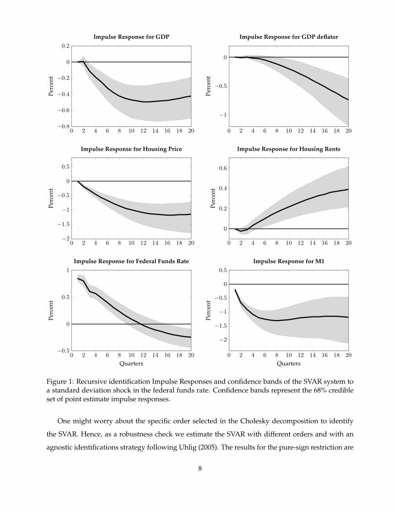
In Figure 1, we show the responses of our six variable benchmark SVAR to a positive standard

deviation shock in the federal funds rate. All the responses are in percentage points on the level

of each variable. Housing rents responds positively after six quarters forward. The initial sluggish

response of housing rents could be the result of stickiness, as housing rents contracts are usually

annual.

The effect of the monetary policy contractionary shock on housing rents is long lasting, reaching

an approximately 0.4% positive response after twenty quarters, five years. The response is large in

magnitude and although not reported here, the response is also significant at a 95% credible set.

If we calculate the accumulated effect on housing rents, we find that a permanent increase of the

federal funds rate by 25 basis points increases housing rents by 1.22% after five years.

The positive response of housing rents happens while output, price level and housing prices

are decreasing. In particular, we find the usual u-shape response of output to a contractionray

monetary policy shock and that housing prices respond in a larger magnitude than rents in the op-

posite direction. The negative effect we find of monetary policy on housing rents confirms previous

literature findings, like Del Negro and Otrok (JME, 2007).

7

0 2 4 6 8 10 12 14 16 18 20−0.8

−0.6

−0.4

−0.2

0

0.2Pe

rcen

t

Impulse Response for GDP

0 2 4 6 8 10 12 14 16 18 20

−1

−0.5

0

Perc

ent

Impulse Response for GDP deflator

0 2 4 6 8 10 12 14 16 18 20−2

−1.5

−1

−0.5

0

0.5

Perc

ent

Impulse Response for Housing Price

0 2 4 6 8 10 12 14 16 18 20

0

0.2

0.4

0.6

Perc

ent

Impulse Response for Housing Rents

0 2 4 6 8 10 12 14 16 18 20−0.5

0

0.5

1

Quarters

Perc

ent

Impulse Response for Federal Funds Rate

0 2 4 6 8 10 12 14 16 18 20

−2

−1.5

−1

−0.5

0

0.5

Quarters

Perc

ent

Impulse Response for M1

Figure 1: Recursive identification Impulse Responses and confidence bands of the SVAR system toa standard deviation shock in the federal funds rate. Confidence bands represent the 68% credibleset of point estimate impulse responses.

One might worry about the specific order selected in the Cholesky decomposition to identify

the SVAR. Hence, as a robustness check we estimate the SVAR with different orders and with an

agnostic identifications strategy following Uhlig (2005). The results for the pure-sign restriction are

8

reported in Figure 2. In the pure-sign identification we restrict the response of inflation and M1 be

negative and federal funds rate to be positive for four periods while the remaining responses are

left unrestricted.

0 2 4 6 8 10 12 14 16 18 20−0.8

−0.6

−0.4

−0.2

0

0.2

Perc

ent

Impulse Response for GDP

0 2 4 6 8 10 12 14 16 18 20−1

−0.5

0

Perc

ent

Impulse Response for GDP deflator

0 2 4 6 8 10 12 14 16 18 20−2

−1

0

Perc

ent

Impulse Response for Housing Price

0 2 4 6 8 10 12 14 16 18 20

0

0.2

0.4

Perc

ent

Impulse Response for Housing Rents

0 2 4 6 8 10 12 14 16 18 20−0.4

−0.2

0

0.2

0.4

Quarters

Perc

ent

Impulse Response for Federal Funds Rate

0 2 4 6 8 10 12 14 16 18 20

−2

−1

0

Quarters

Perc

ent

Impulse Response for M1

Figure 2: Pure-Sign Restriction with k = 4 Impulse Responses and confidence bands of the SVARsystem to a standard deviation shock in federal funds. Confidence bands represent the 68% credibleset of point estimate impulse responses. Here House Prices and Rents are left unrestricted.

The impulse-responses to the contractionary monetary policy shock using the pure-sign restric-

9

tion are qualitatively the same as what we found in the SVAR with the Cholesky decomposition. In

particular, we also find housing rents increase while housing prices fall. However, the responses

are larger in magnitude in the pure-sign restriction. Here, the standard deviation shock in the fed-

eral funds rate is approximately 0.24%, which is close to what is reported in Uhlig (2005), while the

standard deviation in the benchmark SVAR was 0.86%. After accounting for the standardization

of the impulse-response functions (dividing the responses by the standard deviation) we find that

the response of housing rents to a 1% increase in the federal funds rate is 0.46% and 0.83% in the

Cholesky decomposition and pure-sign restriction, respectively.

2.1.2 FAVAR

A. FAVAR Data and Identification

The FAVAR methodology provides a solution to the limited information problem of the SVAR,

and shows that the added information it exploits, help in properly identifying the monetary trans-

mission mechanism. We use quarterly data on 114 time series , that include a broad measures of

prices, production, housing and business activity5 like in Stevanovic (2015) plus our variables of

interest over the 1959Q1- 2006 Q4. All data are assumed stationary or transformed to be covariance

stationary6.

We follow Bernanke, Boivin, and Eliasz (2005) and first use principal components analysis to

construct three factors that provide information about the underlying state of the economy. Sec-

ondly, we treat the Federal funds rate (FFYF) as an observed factor and estimate a SVAR with four

variables: the federal funds rate plus the three factors we estimated using principal components.

The FAVAR naturally allows to overcome some of our missing data. We replace the missing

values with the mean of each variable and use principal components to estimate the factors with

the full dataset. There is no clear way on how one should proceed since not including the full

sample period when data is available to most of the variables can create bias. In our case, the

factors estimation will not be negatively affected by the missing data since it amounts to only 1.6%

of the total data. At the same time, the benefits of adding more information on all other series are

rather large. Hence, we decided to estimate the full sample. In any case, the results are robust if we

use 1983-2006 period.5We thank Dalibor Stevanocic for kindly providing us with the dataset6The principal components analysis requires the data is all in a similar scale and is stationary

10

Another interesting feature of the FAVAR is that we can recover the impulse-responses functions

to any of the data series we are interested in, through the effect of the shock on each factor. This is

made possible by the principal components analyses that decomposes all series by how much they

are explained by factors and by what is unknown. Hence, using the loading factor coefficients we

can then recover the effect of a contractionary monetary policy shock in any variable of interest.

B. FAVAR Results

The FAVAR results confirm our SVAR findings while arguably having a better identification of

the contractionary monetary policy shock. In Figure 3, we present the impulse-response functions of

the variables that constituted the benchmark SVAR to allow an easier comparison between the two

results. Housing rents respond positively to an unexpected increase in the federal funds rate, while

all other sale prices, housing prices and output are falling. Here, the u-shape of output response is

clear and this confirms the neutrality of monetary policy in the long-run.

Housing rents response is initially less sluggish than in the benchmark SVAR but it still only

starts increasing at a higher pace after three to four quarters. Housing prices again respond in a

faster fashion than housing rents. The magnitude of responses is hard to infer directly from the

scale reported in Figure 3 since all variables were standardized in order to use the FAVAR method-

ology. Since, we use the FAVAR just as more of a robustness exercise, we are more interested in the

qualitative behaviour of the impulse-response functions.

To put in a nutshell, our main empirical findings on the effect of monetary policy on housing

rents are housing rents increase after a contractionary monetary policy shock. This result is surpris-

ing and motivates the question on what market mechanism is behind such price dynamics.

We suggest the effect of monetary policy on housing tenure choice, that is, the choice between

owning and renting, can rationalize our empirical findings. in the presence of nominal or financial

frictions, when nominal interest rates increases, the real interest rate increases as well and the real

cost of owning relative to renting increases. Given everything else equal, this may make some

people that are close to be indifferent to prefer to rent instead of buying. If housing supply remains

constant or decreases, this change in consumption behavior leads to an increase of housing rents

relative to all other goods in the economy while all other prices and income fall. We test if the

implications at the aggregate level of such a mechanism are present in the next section.

11

0 2 4 6 8 10 12 14 16 18 20−0.4

−0.3

−0.2

−0.1

0

0.1Pe

rcen

t

Impulse Response for GDP

0 2 4 6 8 10 12 14 16 18 20−0.8

−0.6

−0.4

−0.2

0

0.2

Perc

ent

Impulse Response for GDP deflator

0 2 4 6 8 10 12 14 16 18 20

−0.4

−0.2

0

0.2

Perc

ent

Impulse Response for Housing Price

0 2 4 6 8 10 12 14 16 18 20−0.2

0

0.2

0.4

0.6

0.8

Perc

ent

Impulse Response for Housing Rents

0 2 4 6 8 10 12 14 16 18 20

0

0.1

0.2

Quarters

Perc

ent

Impulse Response for Federal Funds Rate

0 2 4 6 8 10 12 14 16 18 20−0.2

−0.1

0

0.1

0.2

Quarters

Perc

ent

Impulse Response for M1

Figure 3: FAVAR impulse-responses of variables that constituted the benchmark SVAR to a standarddeviation shock in the federal funds rate.

2.2 Evidence on the effect of monetary policy on housing tenure choice

In order to test if the housing tenure choice mechanism is present we show what are the effects

of monetary policy on homeownership rate, homeowner vacancy rate, rental vacancy rate. Again,

we use SVARs and FAVARs to address this question.

12

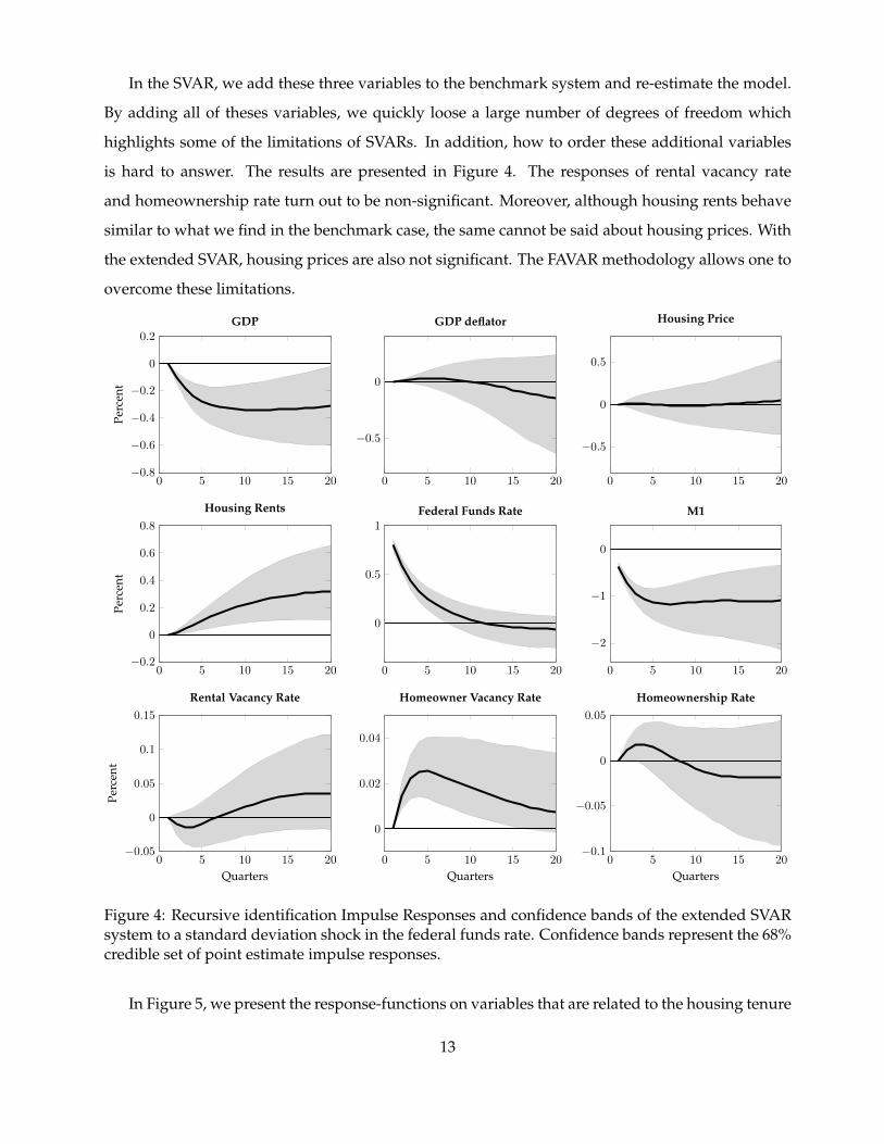
In the SVAR, we add these three variables to the benchmark system and re-estimate the model.

By adding all of theses variables, we quickly loose a large number of degrees of freedom which

highlights some of the limitations of SVARs. In addition, how to order these additional variables

is hard to answer. The results are presented in Figure 4. The responses of rental vacancy rate

and homeownership rate turn out to be non-significant. Moreover, although housing rents behave

similar to what we find in the benchmark case, the same cannot be said about housing prices. With

the extended SVAR, housing prices are also not significant. The FAVAR methodology allows one to

overcome these limitations.

0 5 10 15 20−0.8

−0.6

−0.4

−0.2

0

0.2

Perc

ent

GDP

0 5 10 15 20

−0.5

0

GDP deflator

0 5 10 15 20

−0.5

0

0.5

Housing Price

0 5 10 15 20−0.2

0

0.2

0.4

0.6

0.8

Perc

ent

Housing Rents

0 5 10 15 20

0

0.5

1Federal Funds Rate

0 5 10 15 20

−2

−1

0

M1

0 5 10 15 20−0.05

0

0.05

0.1

0.15

Quarters

Perc

ent

Rental Vacancy Rate

0 5 10 15 20

0

0.02

0.04

Quarters

Homeowner Vacancy Rate

0 5 10 15 20−0.1

−0.05

0

0.05

Quarters

Homeownership Rate

Figure 4: Recursive identification Impulse Responses and confidence bands of the extended SVARsystem to a standard deviation shock in the federal funds rate. Confidence bands represent the 68%credible set of point estimate impulse responses.

In Figure 5, we present the response-functions on variables that are related to the housing tenure

13

choice plus some other variables of interest that are commonly reported in other studies that use

FAVARs. All the results confirm the effect of monetary policy on housing tenure choice. Although,

confidence intervals are not reported here yet, a preliminary one step bootstrap confirmed that all

of the responses are significant at a 68% confidence level.

0 2 4 6 8 10 12 14 16 18 20−0.08

−0.06

−0.04

−0.02

0

0.02

Perc

ent

Homeownership Rate

0 2 4 6 8 10 12 14 16 18 20−0.1

−0.05

0

0.05

0.1

Perc

ent

Homeowner Vacancy Rate

0 2 4 6 8 10 12 14 16 18 20−0.1

−0.05

0

Rental Vancancy Rate

0 2 4 6 8 10 12 14 16 18 20−0.1

−0.08

−0.06

−0.04

−0.02

0

0.02

Perc

ent

Housing Starts

0 2 4 6 8 10 12 14 16 18 20

−0.05

0

0.05

Quarters

Perc

ent

Unemployment Rate

0 2 4 6 8 10 12 14 16 18 20−0.1

−0.05

0

0.05

0.1

Quarters

Capacity Utilization Rate

Figure 5: FAVAR impulse-responses of housing variables, unemployment rate and capacity utiliza-tion rate to a standard deviation shock in the federal funds rate.

We find homeownership rate decreases, which confirms at the aggregate level that more house-

14

holds decide to rent instead of own a house after an unexpected increase in interest rates. Moreover,

we also finds the rental vacancy rate decreases, suggesting that there is a demand pressure on hous-

ing rents and that supply does not seem to keep up making vacancies decrease over total supply of

housing rental. At the same time, the opposite is true to homeowner vacancy rate. Finally, similar

to previous literature Bernanke, Boivin, and Eliasz (2005), we also find that housing starts decrease,

suggesting that housing prices are not falling because of an increase in supply but rather from a

strong decrease in housing demand.

3 New Keynesian Model with Housing Tenure Choice

We extend Clarida, Gali and Gertler (1999) model with endogenous tenure choice decision,

housing prices and housing rents. The inclusion of housing tenure choice in a standard New Key-

nesian model with Taylor rule allow us to derive implications of monetary policy shocks to both

housing prices and rents as well as on homeownership rate. Moreover, by including housing rents,

we can introduce a theoretical CPI in the model that is constructed on housing rents and composite

consumption good. By assuming that a central bank reacts to an imperfect measure of inflation like

CPI, we show how different feedback between inflation and monetary policy is created in a Taylor

rule that responds to CPI instead of inflation. In our model, housing rents increase when interest

rates increase. Hence, central banks over reacts to inflation shocks when they observe an imperfect

measure of inflation like a consumer price index. This effect is worse the larger the share of housing

rents in the consumer price index.

Consider an economy where there is a continuum of households with measure one that live

infinitely and that from time to time make a discrete decision on weather to own or rent a house

when they go to the housing market. There is a fixed probability of re-optimizing on whether to rent

or own a house. This probability is assumed to be the same across all agents, both renters and home

owners. Therefore, a constant mass of households are going to re-optimize every period. Given,

that the mass of households has measure one, the amount of households that re-optimize is just the

probability of re-optimizing. This idea is close in spirit to Calvo (1983) pricing where every period

a fixed share of firms are allowed to re-optimize.

Households are heterogeneous with respect to their preference on the housing services coming

from owning a house. Some agents prefer more than others to live in a house they own instead of

a rented one. This assumption is commonly assumed in the tenure choice literature. The hetero-

15

geneity is needed in order to generate households that rent and households that own their house.

There are alternative ways to introduce heterogeneity in this model that give the same qualitative

implications on the dynamics of the model. Two examples are different households expectations

about future housing prices and heterogeneity in maintenance costs when owning a house. These

alternatives complicate the solution without affecting the results.

We assume that in the initial period of the world only a share of the households are endowed

with housing stock. Moreover, the households that receive housing stock will have initial high debt

so that the initial income is the same across all households. In other words, in the initial period,

some households have housing stock to sell but high debt, and others have no initial housing stock

and no debt. This assumption helps isolating the effects coming from heterogeneity in the hous-

ing market and it makes the model trackable. The interaction of income distribution and housing

distribution would make the model more complicated to solve as we need to keep track of both

distributions over time.

The set of assumptions made in this paper reduces the dimensionality problem while allowing

us to capture the main dynamics of household heterogeneity in the housing market and how this

heterogeneity affects the price dynamics in the housing market. Given income is the same and that

decisions, besides the discrete choice, are not affected by the heterogeneity in households prefer-

ences, we can go from infinite types ex-ante to only two types ex-post. A household type that rents

and other that owns the housing stock. However, the quantity of each type is still endogenous and

that is the main difference to standard models in the literature.

Following Iacoviello (2005) we assume there is a fixed stock of housing in this economy. More-

over we assume the shares of the the total stock that is devoted to rent and owning are also fixed.

By doing so, we abstract from the supply side when we analyse the price dynamics. There are two

main reason that makes one more comfortable with such assumption. First, empirical evidence on

the supply side of housing shows the supply of housing decreases when interest rates increase,

which would make the impact of interest rate on housing prices and rents stronger. The second

reason is we are mainly interested in the dynamics of repeated sales of housing stock. Our main

interest lies on studying how the price of the same housing stock fluctuates over the business cycle.

The stock of houses for owning is owned by the households that bought that housing stock. In

this economy, there exists landlords that own the housing stock for rent and rent it to the house-

holds. Landlords take care of maintenance costs and include them in housing rents that are charged

to any agent type. Hence, households do not face any maintenance cost when renting a house. We

16

assume all agents have fixed equal shares of the landlords firms and thus receive the same amount

of profits coming from renting housing.

In our environment, households go on their respective housing market every period. That is, if

you are a renter you go to the housing rental market and decide on how much to rent every period.

And if you are a owner, you sell the stock you had from previous period and decide on how much

to buy again. However, sometimes the households are going to re-optimize and decide on whether

he wants to rent or own a house. There are many reasons why come household would do so, but

we abstract from this exercise. Here, we just assume households do not re-optimize every period.

The production side of the economy is similar to Clarida Gali and Gertler (1999). There is a

continuum of intermediate monopolistic firms who produce using labor only and sell their product

to be used as an input by the final good firms, and are subject to sticky prices. . Final good firms

produce using intermediate goods varieties only. The monopolistic intermediate firms on the con-

sumption sector are the source of nominal rigidity while housing prices and rents are assumed to be

flexible. Finally, there is a monetary authority that obeys a Taylor rule when setting interest rates.

A. Households

Households decide on how much to consume of the composite consumption good and hous-

ing services, and finally on how much to borrow with nominal bonds. Households supply labor

ineslastically and receive a nominal wage Wt for their total labor. On the one hand. if the house-

hold decides to own a house, he pays Qt for each unit of housing services7. On the other hand, if

the household decides to rent a house, he pays Rt. Finally, households receive/pay gross nominal

interest It on their nominal bonds. The households have to choose between renting and owning a

house. Once they decide to rent or own they are stuck with that decision until they can re-optimize

again. Therefore, to make this choice, they compare how much utility they receive from each al-

ternative, and choose the one that yields the highest discounted utility to them. The utility is both

discounted by time preference of consumption and the probability of re- optimizing. Let V denote

the indirect utility function, the agent will choose to rent or own depending on which choice gives

him the highest level of utility.

maxrent,own

(V ∗rent, V∗own)

7We assume for simplicity that each unit of housing stock provides exactly one unit of housing services.

17

When households decide to rent, note that there is no heterogeneity and hence their decision is

the same among the households who decide to rent. Their problem can be described as:

maxct,ht,bt+1,Nt

E0

∞∑t=0

(γβ)t(ln ct + α ln ht − exp(τt)N1+ηt

1 + η)

s.t.

ct + Ltht + bt = at

at = WtNt + Πt +O(ownedt−1)(Itπtbt−1 +Qtht−1)

given h0, b0

(1)

Where τ is an exogenous preference shock to leisure and at stands for the household net worth.

The indicator functionO takes the value one if he households owned a house in the previous period.

If he did, he is going to have a debt associated with that purchase that offsets the value of the

house. Hence, we assume that the net worth of the agents who are considering renting is the same

regardless of whether the household owned a house or not in the previous period. Also, when

renting, households do not own the housing stock and hence cannot sell the housing stock in the

next period. In our model, we implicitly assume that landlords take care of any type of maintenance.

Solving for the first order conditions of this maximization problem we get the following Euler

equations:

c−1t = γβEt[

It+1

πt+1c−1t+1] (2)

α

ht=

Ltct

(3)

exp(τt)Nηt ct = Wt (4)

Equation (2), the first Euler equation represents the typical dynamic trade-off between consump-

tion now and future consumption. This trade-off is a direct result from the savings decision. The

second Euler equation (3) represents the new feature of our model, and it shows the trade-off be-

tween consumption of the composite final good and housing services. Finally, the third Euler equa-

tion (4) represents the trade-off between leisure and consumption.

18

When the households decide to own a house, their problem is to:

maxct,ht,bt,Nt

E0

∞∑t=0

(γβ)t(ln ct + α lnht − exp(τt)N1+ηt

1 + η− ρi)

s.t.

ct +Qtht + bt = at

at = WtNt + Πt + I(ownedt−1)(Itπtbt−1 +Qtht−1)

given h0, b0

(5)

Solving for the first order conditions of this maximization problem we get the following Euler

equations:

c−1t = γβEt[

It+1

πt+1c−1t+1] (6)

α

ht=

1

ct

(Qt −

Qt+1

It+1/πt+1

)(7)

exp(τt)Nηt ct = Wt (8)

Given the optimal decisions coming from both tenure choices, households will choose the one

that gives him more utility. Moreover, assuming the net worth is the same and given our log utility

function, the only difference between the tenure decisions is going to be the amount of housing

services and consumption. Hence we have households will rent if:

V ∗rent = E0

∞∑t=0

(γβ)t(ln c∗t + α ln h∗t ) > E0

∞∑t=0

(γβ)t(ln c∗t + α lnh∗t − ρi) = V ∗own

Hence, using (3) and (6) and simplifying we have that the indifferent household is given by the

following equality:

E0

∞∑t=0

(γβ)tLth1+αt = E0

∞∑t=0

(γβ)t((

Qt −Qt+1

It+1/πt+1

)h1+αt − ρt

)(9)

ρt = (1− γβ)E0

∞∑t=0

(γβ)t((

Qt −Qt+1

It+1/πt+1

)h1+αt − Lth1+α

t

)(10)

19

The household that is indifferent between renting and owning pins down how many households

are going to rent and own a house in equilibrium. Households that prefer to own a house at a level

ρi < ρ, will decide to own a house while households they have ρi > ρ will rent. Note that the cutoff

rule ρ is endogenous and depends on prices and allocations.

B. Firms

The firm problem in our model is standard in the New Keynesian framework. We use a contin-

uum of intermediate monopolistic firms together with Calvo pricing mechanism that use only labor

input in production.

Each household buys their consumption good from final good firms. The final good firms buy

Yit from the intermediate sector for Pit and sell their production to the households for Pt. The

technology of production of the final good firms is given by:

Yt =

(∫ 1

0Yit

1− 1ε dk

) εε−1

, ε > 1 (11)

Individual demand for each intermediate firms product is given by:

Yit =

(PitPt

)−εYt (12)

Equations (11) and (12) imply that:

Intermediate firms demand labor and their production technology is given by:

Yit = AtNt(k) (13)

In our model nominal rigidity is imposed like in Calvo (1983) whereby a fraction of firms, 1− θ,

is allowed to reset price each period. The problem is symmetric and so all firms that can re-optimize

choose P ∗t to solve:

maxP ∗t

E0

∞∑τ=0

θτ{νt+τ (P ∗t Yi,t+τ − Φt+τ |Yt+τ |t

}(14)

Where Φt+τ is the marginal cost at a specific level of production. The profits of the intermediate

firms are transfers to the households. The details of the derivations of P ∗ in a nonlinear fashion can

be found in Christiano (2011).

20

As a fraction of prices stays unchanged, the aggregate price level evolution is;

Pt = (θP 1−εt−1 + (1− θ)P ∗t

1−ε)1/(1−ε) (15)

If we do a first order approximation around the steady state on Equation (15) together with the

solution to (14), we get the forward-looking Phillips curve. In our case, we will do a second order

approximation because agents use welfare when deciding to own or rent. Hence, we a second order

approximation around steady state in order to have an accurate solution of the model.

C. Consumer Price Index

With the explicit introduction of housing rents, we can formalize the implied consumer price

index in our model economy. The consumer price index in going to be a weighted average of

nominal prices of housing and non-housing goods. We assume the weight a of 0.3 on housing

shelter that is the same as in the data CPI. Hence we have CPI inflation is given by:

CPIt = aPtPt−1

+ (1− a)PtPt−1

LtLt−1

(16)

The consumption good real price is 1 and hence the price variation is given by monetary infla-

tion. However, housing rents nominal change of prices is a composition of monetary inflation and

real housing rents inflation. From equation (16) it is clear that CPI gives a guidance on how mon-

etary inflation behaves in trend if real prices behave like some white noise. However, if real prices

change strongly and persistently in opposite directions, CPI becomes noisy as a measure of mon-

etary inflation. This model provides a formal way to start thinking about how monetary inflation

should be measured, and goes in the direction of providing insights to the points raised in Vining

and Elwertowski (1976).

D. Central Bank

The central bank implements a Taylor-type of interest rate rule. Hence, central bank reacts to

output gap and inflation gap according to:

It = (It−1)φI (CPI1+φπt−1 (Yt−1/Y )φY r)1−φIeI,t (17)

21

We assume all agents in the economy measure well monetary inflation and know the central

bank targets the implied CPI with housing rents. In the counterfactual section we show how this

economy differs from one where the central bank reacts to a CPI that is rents-free.

E. Exougenous Shocks

In our model economy τt has follows an AR(1) process:

τt = ρττt−1 + eτ,t (18)

Hence, there are two kinds of shocks: a preference on leisure shock eτ,t and a monetary policy

shock eI,t. Both shocks follow a normal distribution eτ,t ∼ N(0, στ ) and eI,t ∼ N(0, σI), respectively.

F. Market Clearing

The market clearing conditions in our economy are the following:

Goods Market

γ

∫ ρt−1

0ctdi+ (1− γ)

∫ ρt

0ctdi+ γ

∫ 1

ρt−1

ctdi+ (1− γ)

∫ 1

ρt

ctdi = Wt + Πt ∀t (19)

Labor Market

∫ 1

0Njtdj = Nt ∀t (20)

Homeowners housing market

γ

∫ ρt−1

0htdi+ (1− γ)

∫ ρt

0htdi = HO ∀t (21)

Rental housing market

γ

∫ 1

ρt−1

htdi+ (1− γ)

∫ 1

ρt

htdi = HR ∀t (22)

Nominal Bonds Market

22

γ

∫ ρt−1

0btdi+ (1− γ)

∫ ρt

0btdi+ γ

∫ 1

ρt−1

btdi+ (1− γ)

∫ 1

ρt

btdi = 0 ∀t (23)

G. Equilibrium

Definition. The Rational Expectations Competitive Equilibrium is a sequence household choices {ct, ct, ht, ht,

bt+1, bt+1, Nt}∞t=0, a sequence of housing tenure choice (rent vs own) {oi}∞t=0, profits and transfers {Πt}∞t=0

,a cut-off preference level that makes the households indifferent between renting and owning {ρt}∞t=0 and a

sequence of prices {Wt, Qt, Lt, Pt, P∗t CPIt, It}∞t=0 such that:

1) Given prices and profits, {ct, ht, bt+1, Nt}∞t=0 solves the households problem when owning and {ct, ht, bt+1, Nt}∞t=0

solves the households problem when renting.

2) Given prices and allocations, {ρt}∞t=0 solves equation (10).

3) Given prices and allocations, {P ∗t }∞t=0 solves (10) and profits {Πt}∞t=0 are the associated indirect func-

tion (14) with optimal price {P ∗t }∞t=0.

4) Given allocations, {Wt, Qt, Lt}∞t=0 solve market clearing (19), (20), (21), (22) and (23).

5) Given prices and allocations, {Pt}∞t=0 solves equation (15), {CPIt}∞t=0 solves equation (16) and{It}∞t=0

solves equation (17).

4 Calibration and Solution

We calibrate the model to match long-term moments of the US economy. All parameter values

are taken form previous literature on New Keynesian models like Iacoviello (2005), Clarida, Gali

and Gertler (1999) and Christiano, Eichenbaum and Evans (2005). In Table 1 we show the param-

eters values. The inter-temporal discount factor was selected to match the US steady state annual

interest rate approximately.

The parameter that governs the labor supply aversion with a value of 0.01 implies a practically

flat labor supply. This is higher than what microeconometric studies suggest, but it is consistent

with the weak observed response of real wages to macroeconomic disturbances and moreover can

be motivated by the changes in labor supply coming from the extensive margin. That is the amount

23

Description Parameter Value

Preferences

Discount Factor γβ 0.99

Weight on housing services α 0.10

Labor Supply Aversion η 0.01

Sticky Prices

Steady State Markup X 1.20

Probability of fixed price θ 0.75

CPI

Housing Rents Share in CPI a 0.30

Taylor Rule

Interest Rate Smoothing φI 0.80

Reaction to Inflation Gap φπ 1.50

Reaction to Output Gap φY 0.10

Exogenous Shocks

Persistence of Leisure Preference Shock ρτ 0.90

Leisure Preference Shock Std. Dev. στ 0.010

Interest Rate Shock Std. Dev. σI 0.007

Table 1: Benchmark model calibrated parameters. All parameters are selected from previous litera-ture on standard New Keynesian models like Clarida, Gali and Gertler (1999), Christiano, Eichen-baum and Evans (2005), and Iacoviello (2005).

of individuals that change from unemployed to employed, even though hours works do not change

much for individuals at work.

The preference parameter on housing services is justified by Iacoviello (2005). Our preferences

are the same the exception that we do not model explicitly money. However, money has a insignifi-

cant impact on utility function in Iacoviello (2005), which is typically the case in money in the utility

models. The markup is taken from Christiano, Eichenbaum and Evans (2005). The housing rents

share in CPI is around 30%. The Taylor rule parameters are taken from Clarida, Gali and Gertler

(1999) and are similar to those used by Iacoviello (2005). These parameters imply a Taylor rule that

describes well monetary policy post Volcker period. Finally, the shock on monetary policy was

calibrated to match the initial response of interest rates of the benchmark SVAR.

The model is solved using a perturbation method with a second order approximation around

24

the steady state. The second order approximation in our model is crucial because agents compare

lifetime utility function when deciding on whether to own or rent a house. It is well known that

first order approximations give inaccurate solutions to welfare analysis because they miss second

moments. Hence, with the second order approximation and small shocks we are able to accurately

solve the model.

Although our model is highly stylised, Table 2 shows the models performs remarkably well in

matching long term moments like ownership rate and price to rent ratio, as well as business cycle

moments. Although the source of heterogeneity in our model comes only from preferences and the

housing supply side is introduced in a very simple way, the homeownership rate we get from our

model is close to the data. Our preferences heterogeneity is in some sense a reduce form approach

to what drives the homeownership rate. For the fundamentals behind the homeownership rate

and the price to rent ratio see Chambers, Garriga, and Schlagenhauf (2009), Sommer, Sullivan and

Verbrugge (2013) and Miao, Wang and Zha (2014). Moreover, the price to rent ratio is also similar

to the average price to rent ratio found in the data, which suggest supply dynamics do not seem to

be important in matching long term housing tenure choices dynamics.

Moments Model Data

Steady State

Homeownership rate 0.70 0.64

Price-Rent Ratio 23.29 18.80

Business Cycle

CPI Std. Dev. 0.025 0.015

Output Std. Dev. 0.099 0.014

Housing Prices Std. Dev. 0.103 0.054

Housing Rents Std. Dev. 0.0083 0.0069

Table 2: Model versus Data comparison of moments that were not targeted

Besides housing prices standard deviation , the model business cycles standard deviation matches

well the data. The model predicts housing prices that almost doubles that of the data. One reason

can be the missing housing market fundamentals in the model and another reason might be the lack

of stickiness in housing rents. Housing rents are very sticky in reality and in our model they are

assume flexible. Given how our mechanism for homeownership works, if rents do not respond as

strongly specially when decreasing (housing rents stickiness is not symmetric), housing prices will

not change as abruptly and this will dampen housing prices volatility.

25

With the model calibrated we show the theoretical impulse-response functions in Figure 6. The

tenure choice mechanism enables the New Keynesian model to opposite responses of housing prices

and housing rents in response to a monetary monetary contractionary shock. Housing prices de-

crease and housing rents increase after nominal interest rates increase. This result is puzzling if

one thinks of housing as an asset only. However, housing is also a consumption good and utility

considerations are hence important in determining prices. If houses are just assets, one would ex-

pect housing prices are nothing but the present value of all future housing rents. Hence, changes in

interest rates would have to change both housing prices and rents in the same direction. However,

housing is not just an asset and households buy housing stock not just to rent it but also to consume

it. Hence, there is a dichotomy between rents and housing prices.

Moreover, with heterogeneous agents, households have different valuations for the same hous-

ing stock. When interest rate increase, more agents prefer to rent instead of owning creating a

change in housing demand in the extensive margin. We can see in Figure 6 that indeed this is the

case looking at how homeownership rate decreases after interest rates rise.

The consideration of housing rents allows us to introduce a theoretical consumer price index.

We can see in Figure 6 that CPI increases in spite of the fact monetary inflation decreases. This

is the result of rising rents that is sufficiently large to overcome the drop in monetary inflation.

CPI then decreases since housing rents start decreasing. Interestingly, when CPI is targeted by the

Taylor rule, monetary inflation first decreases and then increases above steady state. Since, the

monetary authority overshoots interest rates households cut consumption sharply. As a response

to the drop in demand, firms first cut down employment and decrease prices to maintain the fixed

markup. However, households and firms know the monetary authority is targeting CPI, and once

CPI behaves normally, they know the interest rates are going to quickly drop making them increase

consumption. Firms again increase employment and prices increase given the higher wages. The

employment and output responses can be found in the appendix of this paper in Figure 10.

Looking at Figure 7, we can see that the model impulse responses matches well the SVAR im-

pulse response functions. Housing rents increase while housing prices and output fall. Moreover,

we are able to match the “price puzzle” that commonly appears in the SVAR literature on monetary

policy. Hence, looking at a theoretical measure that allows to construct a price index similar to a

CPI, there is no puzzle in a rising CPI while nominal inflation is decreasing. This happens because

the rise in housing rents out weights the decrease in nominal inflation. We explore this insight in

Dias and Duarte (2015) and show that the price puzzle is largely explained by housing rents. Our

26

0 2 4 6 8 10 12 14 16 18 20

−1

−0.5

0

Perc

ent

Q - Housing Price

0 2 4 6 8 10 12 14 16 18 200

0.2

0.4

0.6

0.8

1

L - Housing Rent

0 2 4 6 8 10 12 14 16 18 20−0.03

−0.02

−0.01

0

Perc

ent

ρ - Homeownership Rate

0 2 4 6 8 10 12 14 16 18 200

0.2

0.4

0.6

0.8

1I - Nominal Interest Rate

0 2 4 6 8 10 12 14 16 18 200

0.2

0.4

Perc

ent

CPI - Consumer Price Index

0 2 4 6 8 10 12 14 16 18 20−0.2

−0.1

0

π - Inflation

Figure 6: Impulse-Response functions for main variables of interest for the benchmark model wherethe Taylor rule targets CPI. Each graph shows percentage-point response of one of the model’svariables to a one-standard-deviation shock in monetary policy.

results suggest a mechanism that can generate the price puzzle different from the so called channel

cost of monetary policy (Barth and Ramey (2001)) and Christiano, Eichenbaum and Evans (2005).

To test this hypothesis, Rabanal (2006) estimates a New Keynesian model of the business cycle and

tests the conditions under which a cost channel of monetary policy could generate a positive re-

sponse of prices to a contractionary monetary policy shock. This author finds that, demand side

effects always dominate supply side effects in prices and therefore there is no evidence that the cost

channel of monetary policy could explain the price puzzle. Our results provide some insights on

the type of demand shocks that drive the response of prices.

The fit is particularly not good in the first periods. This is mainly due to the identification

assumption of the SVAR. We are faced with a trade-off, we either make an identification ordering

27

0 2 4 6 8 10 12 14 16 18 20−1

0

1Pe

rcen

t

Federal Funds Rate

SVARModel

0 2 4 6 8 10 12 14 16 18 20

−0.2

0

0.2

0.4

CPI

0 2 4 6 8 10 12 14 16 18 20−4

−2

0

Perc

ent

Housing Prices

0 2 4 6 8 10 12 14 16 18 20−1

−0.5

0

0.5

1

Real Housing Rents

0 2 4 6 8 10 12 14 16 18 20−2

0

2

Quarters

Perc

ent

GDP

Figure 7: Impulse-Response functions for main variables of interest for the benchmark model wherethe Taylor rule targets CPI versus SVAR with Choleski identification that is consistent with themodel. Each graph shows percentage-point response of one of the model’s variables to a one-standard-deviation shock in monetary policy.

that is consistent with the timing assumptions of the model, or we get a better identification. This

trade-off was also faced by Iacoviello (2005). We decided to follow Iacoviello (2005) and opted for

the former one by sacrificing some identification to make the SVAR more consistent with the model.

Hence, given that in the model all variables respond contemporaneously to shocks in interest rates,

we order the federal funds rate first in the SVAR. Besides, the initial periods, the economy behaves

similarly to the SVAR. Finally, it is worth noting that rents are flexible in the model while in reality

rents are very sticky as shown by the SVAR response of housing rents. If our model had rents being

28

stick like the data, our theoretical CPI would be able to be always positive like in the data. For more

details on the price puzzle see Dias and Duarte (2015).

5 Counterfactual - CPI versus CPI net of rents

Here, we ask the question on how the dynamics of the model in the benchmark case compare

to the alternative setting, where the monetary authority targets a rents-free consumer price index.

Note that the rents-free price index is just the usual monetary inflation studied in most of the stan-

dard New Keynesian models.

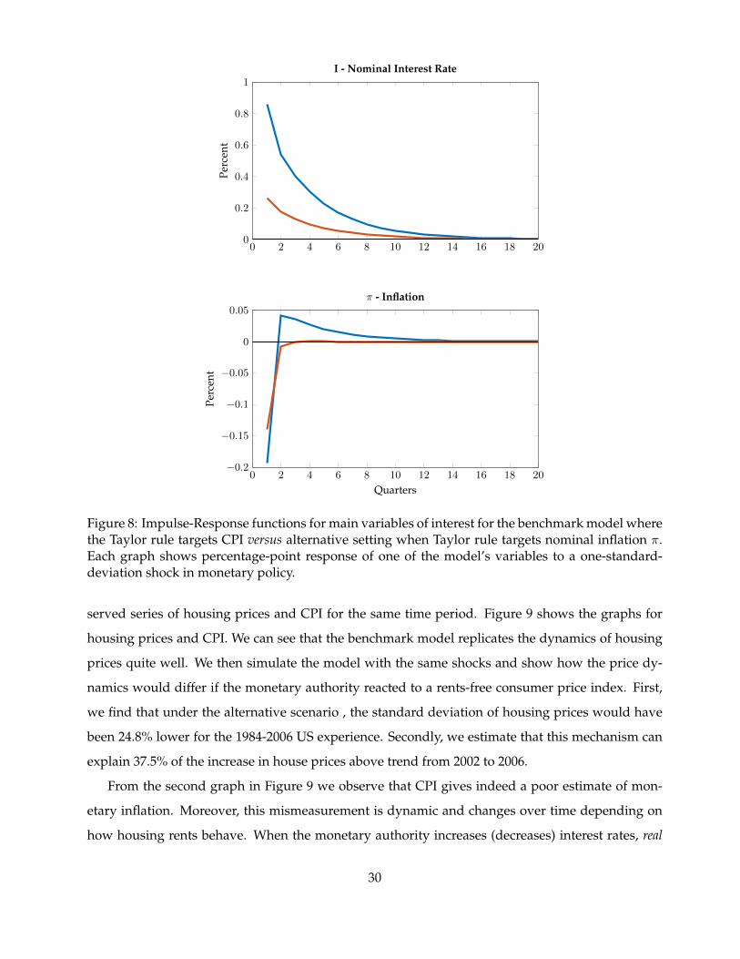
We show in Figure 8 the impulse responses of the two different cases. In the alternative case,

where the monetary authority targets the rents-free CPI, interest rates will be lower than in the

benchmark as a response to the same shock. This happens because when the monetary authority

targets the consumer price index with housing rents, CPI will be initially above the target, and

hence interest rates will be set too high to bring CPI to the target. The increase in CPI is in turn

driven by rising housing rents. Although the differences are small in a response to a single shock,

these differences can become rather large when accumulating different shocks to the economy over

time. Moreover, if rents were sticky, CPI distortions would be much larger in later periods. Real

interest rate is similar with the exception of the first period.

When interest rate Taylor rules use the CPI as an input, interest rates will be set too high based

on rising rents instead of nominal inflation and will add unnecessary variation to the underlying

inflation rate. This generates large welfare costs and losses to a monetary policy whose objective is

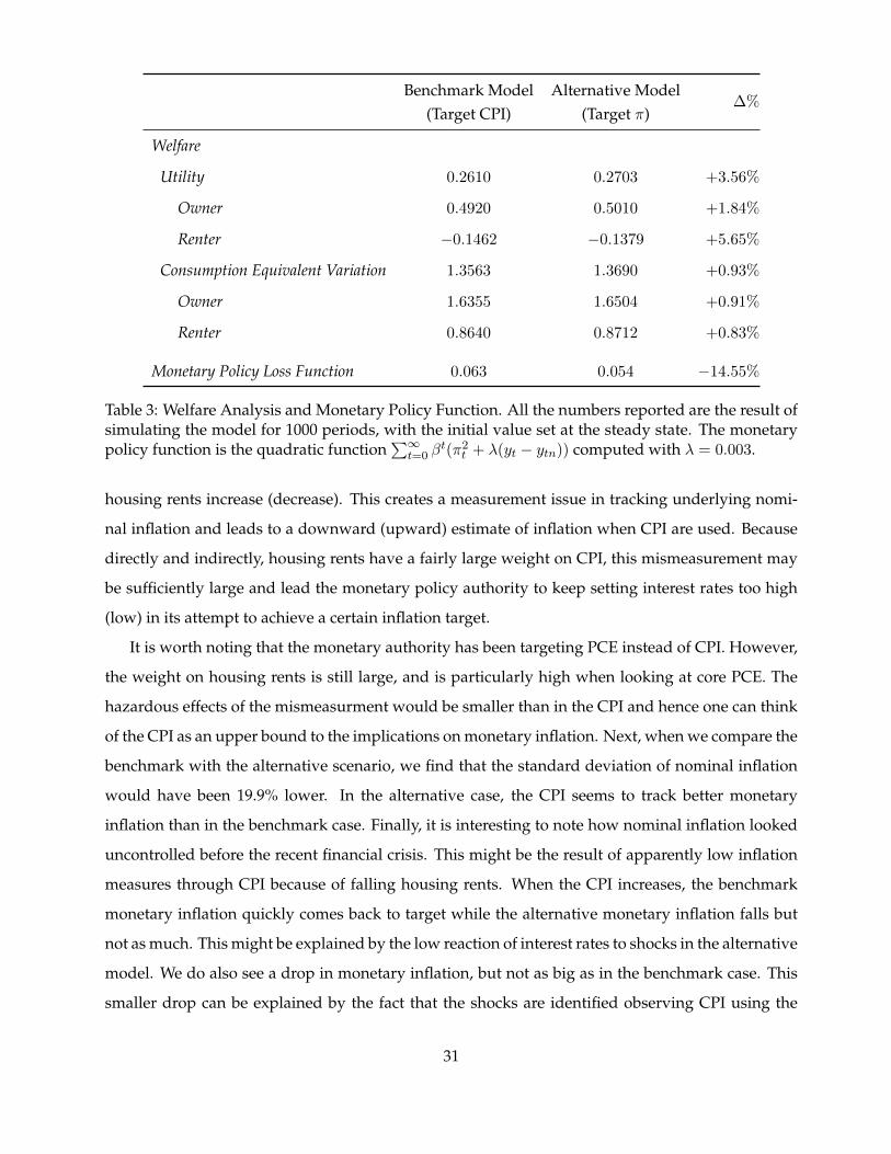
to minimize inflation and output gap variance. Table 3 reports the welfare analysis. We simulate

the model with monetary policy shocks for one thousand periods. We find that targeting a measure

of inflation that excludes housing rents leads to a 0.9% welfare gain in consumption equivalent

variation and to a 14.5% fall in the loss function of monetary policy in comparison to the case that

the monetary authority targets a measure of inflation that includes housing rents. Households are

affected differently. Owners are affect more in consumption equivalent variation because housing

prices are more volatile to interest rate shocks than housing rents.

Finally, using the same counterfactual, we answer how prices dynamics might have been differ-

ent for the U.S. experience between 1984 and 2006. With two shocks, we assume that only housing

prices and CPI are observable. Then, using the Kalman filter with the calibrated parameters we

are able to recover the monetary policy and preference shocks for the 1984-2006 by matching ob-

29

0 2 4 6 8 10 12 14 16 18 200

0.2

0.4

0.6

0.8

1

Perc

ent

I - Nominal Interest Rate

0 2 4 6 8 10 12 14 16 18 20−0.2

−0.15

−0.1

−0.05

0

0.05

Quarters

Perc

ent

π - Inflation

Figure 8: Impulse-Response functions for main variables of interest for the benchmark model wherethe Taylor rule targets CPI versus alternative setting when Taylor rule targets nominal inflation π.Each graph shows percentage-point response of one of the model’s variables to a one-standard-deviation shock in monetary policy.

served series of housing prices and CPI for the same time period. Figure 9 shows the graphs for

housing prices and CPI. We can see that the benchmark model replicates the dynamics of housing

prices quite well. We then simulate the model with the same shocks and show how the price dy-

namics would differ if the monetary authority reacted to a rents-free consumer price index. First,

we find that under the alternative scenario , the standard deviation of housing prices would have

been 24.8% lower for the 1984-2006 US experience. Secondly, we estimate that this mechanism can

explain 37.5% of the increase in house prices above trend from 2002 to 2006.

From the second graph in Figure 9 we observe that CPI gives indeed a poor estimate of mon-

etary inflation. Moreover, this mismeasurement is dynamic and changes over time depending on

how housing rents behave. When the monetary authority increases (decreases) interest rates, real

30

Benchmark Model Alternative Model∆%

(Target CPI) (Target π)

Welfare

Utility 0.2610 0.2703 +3.56%

Owner 0.4920 0.5010 +1.84%

Renter −0.1462 −0.1379 +5.65%

Consumption Equivalent Variation 1.3563 1.3690 +0.93%

Owner 1.6355 1.6504 +0.91%

Renter 0.8640 0.8712 +0.83%

Monetary Policy Loss Function 0.063 0.054 −14.55%

Table 3: Welfare Analysis and Monetary Policy Function. All the numbers reported are the result ofsimulating the model for 1000 periods, with the initial value set at the steady state. The monetarypolicy function is the quadratic function

∑∞t=0 β

t(π2t + λ(yt − ytn)) computed with λ = 0.003.

housing rents increase (decrease). This creates a measurement issue in tracking underlying nomi-

nal inflation and leads to a downward (upward) estimate of inflation when CPI are used. Because

directly and indirectly, housing rents have a fairly large weight on CPI, this mismeasurement may

be sufficiently large and lead the monetary policy authority to keep setting interest rates too high

(low) in its attempt to achieve a certain inflation target.

It is worth noting that the monetary authority has been targeting PCE instead of CPI. However,

the weight on housing rents is still large, and is particularly high when looking at core PCE. The

hazardous effects of the mismeasurment would be smaller than in the CPI and hence one can think

of the CPI as an upper bound to the implications on monetary inflation. Next, when we compare the

benchmark with the alternative scenario, we find that the standard deviation of nominal inflation

would have been 19.9% lower. In the alternative case, the CPI seems to track better monetary

inflation than in the benchmark case. Finally, it is interesting to note how nominal inflation looked

uncontrolled before the recent financial crisis. This might be the result of apparently low inflation

measures through CPI because of falling housing rents. When the CPI increases, the benchmark

monetary inflation quickly comes back to target while the alternative monetary inflation falls but

not as much. This might be explained by the low reaction of interest rates to shocks in the alternative

model. We do also see a drop in monetary inflation, but not as big as in the benchmark case. This

smaller drop can be explained by the fact that the shocks are identified observing CPI using the

31

1984 1985 1986 1987 1988 1989 1990 1991 1992 1993 1994 1995 1996 1997 1998 1999 2000 2001 2002 2003 2004 2005 2006−10

−5

0

5

10

15Pe

rcen

t

Data and Model Simulated Real Housing Prices Business Cycles

DataBenchmark - CPI TargetAlternative - π Target

1984 1985 1986 1987 1988 1989 1990 1991 1992 1993 1994 1995 1996 1997 1998 1999 2000 2001 2002 2003 2004 2005 2006−4

−2

0

2

4

6

Perc

ent

CPI and Model Simulated Inflation

CPI in dataπ in benchmark modelπ in alternative model

Figure 9: Housing Prices Business cycle on top and CPI business cycle for data from 1984 to 2006with simulated data form the benchmark and simulated model. All business cycles are computedusing a HP filter. In the model, by assuming we only observe housing prices and CPI we extract theimplied monetary policy and preference shocks using Kalman Filter. We use the recovered shocksto simulate the model.

benchmark case.

6 Conclusion

In this paper we unveil a new channel through which housing reveals its importance in the

economy by investigating the interaction between monetary policy and housing rents. Using SVARs

and FAVARs, we first show housing rents respond positively to a contractionary monetary policy

shock. Secondly, recognizing housing rents directly and indirectly account for about 30% of CPI,

32

we show our first finding brings new insights on inflation measurement and strong implications to

the way monetary policy is conducted. We propose and calibrate a DSGE model that endogeneizes

housing tenure choice and is both able to explain the empirical findings and provide answers for

monetary policy experiments.

Counterfactual exercises reveal that when the Taylor rule uses the CPI as an input, interest rates

will be set too high based on rising rents instead of currency inflation. This generates large welfare

costs, adds unnecessary variation to the underlying monetary inflation rate and losses to a monetary

policy whose objective is to minimize inflation and output gap variance. Finally, by simulating

the model we find monetary policy based on CPI explains a large proportion of the housing price

business cycle boom that preceded the 2008 financial crisis.

We do not make the case for the exclusion of housing rents from the consumer price indexes in

every circumstance. Housing rents are an important item on measuring households cost of living

since households spend around 30% of their income with shelter, and hence should be included.

In general, price indexes trends capture well the evolution of the nominal state of the economy.

However, when relative prices of some specific goods change suddenly, the consumer prices in-

dexes are affected regardless of how underlying monetary inflation behaves. Given that we show

housing rents relative price is strongly affected by monetary policy and that housing rents have a

large weight in the consumer price indexes, care should be in place when interpreting the response

of consumer price indexes to monetary policy shocks as purely monetary inflation.

33

References

Barth, Marvin J., and Ramey, Valerie A., “The Cost Channel of Monetary Transmission”,

NBER Macroeconomics Annual, 2001.

Bernanke, Ben S., Boivin, Jean, Eliasz, Piotr, “Measuring the Effects of Monetary Policy: A

Factor-Augmented Vector Autoregressive (FAVAR) Approach”, The Quarterly Journal of Eco-

nomics, 2005, Volume 120 (1), Pages 387-422.

Boskin, Michael J., Dulberger, Ellen R. , Gordon, Robert J., Griliches, Zvi and Jorgenson,

Dale W. “Consumer Prices, the Consumer Price Index, and the Cost of Living ”, The Journal

of Economic Perspectives, 1998, Vol. 12, No. 1, Pages 3-26.

Calvo, Guillermo A., Eichenbaum, Martin and Evans, Charles, “Staggered Prices in a Utility-

Maximizing Framework”, Journal of Monetary Economics, 1983, Volume 12, Pages 383-398.

Chambers, Matthew, Garriga, Carlos and Schlagenhauf, Don E., “Accounting for Changes

in the Homeownership Rate ”, International Economic Review, 2009, Vol. 50, No. 3, Pages

677-726.

Christiano, Lawrence J., “Simple New Keynesian Model without Capital ”, NBER course, 2011.

Christiano, Lawrence J., Eichenbaum, Martin and Evans, Charles, “Monetary Policy Shocks:

What Have We Learned and to What End?”, NBER Working Paper No. 6400, 1998.

Christiano, Lawrence J., Eichenbaum, Martin and Evans, Charles, “Nominal Rigidities and

the Dynamic Effects of a Shock to Monetary Policy ”, Journal of Political Economy, 2005, Vol.

113, No. 1, Pages 1-45.

Church, Jonathan D., “Explaining the 30-year shift in consumer expenditures from commodi-

ties to services, 1982-2012. Montlhy Labor Review, April 2014.

Clarida, Richard, Gali, Jordi, and Gertler, Mark “The Science of Monetary Policy: A New

Keynesian Perspective ”, Journal of Economic Literature, 1999, Vol. 37, no. 2, Pages 1661-1707.

Clark, Todd E., “Comparing Measures of Core Inflation”, Economic Review, 2001, Second Quar-

ter, Pages 5-31.

34

Coibion, Olivier, Gorodnichenko, Yuriy, Kueng, Lorenz, and Silvia, John, “Innocent By-

standers? Monetary Policy and Inequality in the U.S.”, NBER Working Paper , 2012, No.

18170.

Del Negro, Marco, and Otrok, Christopher “99 Luftballons: Monetary policy and the house

price boom across U.S. states ”, , Journal of Monetary Economics, 2007, Volume 54, Pages

1962–1985.

Dias, Daniel A. and Duarte, Joao B. “The effect of monetary policy on housing tenure choice

as an explanation for the price puzzle ”, mimeo UIUC, 2015.

Dıaz, Antonia and Luengo-Pradob, Marıa Jose “On the user cost and homeownership ”, ,

Review of Economic Dynamics, 2008, Volume 11, Issue 3, Pages 584–613.

Gordon, Robert J. and vanGoethem, Todd “Downward Bias in the Most Important CPI Com-

ponent: The Case of Rental Shelter, 1914–2003 ”, NBER, 2007.

Henderson, J. V. and Ioannides, Y. M. “A Model of Housing Tenure Choice”, American Eco-

nomic Review, 1983, Volume 73, No.1, Pages 98-113.

Iacoviello, Matteo “House Prices, Borrowing Constraints, and Monetary Policy in the Business

Cycle”, American Economic Review, 2005, Vol. 95, No. 3 (June), Pages 739-764.

Iacoviello, Matteo, and Pavan, Marina “Housing and Debt over the Life Cycle and over the

Business Cycle ”, Journal of Monetary Economics, 2013, March, vol. 60(2), Pages 221-238.

Leamer, Edward E. “Housing is the Business Cycle ”, NBER working paper, 2007, No. 13428.

Miao, Jianjun, Wang, Pengfei, and Zha, Tao, “Liquidity Premia, Price-Rent Dynamics and

Business Cycles ”, NBER Working Paper, 2014, No. 20377.

Rabanal, Pau, “Does inflation increase after a monetary policy tightening? Answers based

on an estimated DSGE model”, Journal of Economics Dynamics & Control, 2006, Volume 31,

Pages 906-937.

Sims, Chris A. “Interpreting the macroeconomic time series facts: the effects of monetary pol-

icy”, European Economic Review, 1992, Volume 36 (5), Pages 975-1000.

35

Sommer, Kamila, Sullivan, Paul and Verbrugge, Randal “The equilibrium effect of funda-

mentals on house prices and rents”, Journal of Monetary Economics, 2013, Volume 60, Pages

854–870.

Uhlig, Harald “What are the effects of monetary policy on output? Results from an agnostic

identification procedure ”, Journal of Monetary Economics, 2005, Volume 52, Pages 381-419.

Vining , Daniel R., and Elwertowski, Thomas C. “The Relationship between Relative Prices

and the General Price Level ”, American Economic Review, 1976, Vol. 66, No. 4 Pages 699-708.

36

Appendix

A - Figures

0 5 10 15 20

−1

−0.5

0

Perc

ent

Y - Output

0 5 10 15 20−0.2

−0.1

0

N - Employment

0 5 10 15 20−10

−8

−6

−4

−2

0

Perc

ent

hhat - Housing Services Renter

0 5 10 15 200

1

2

3

4

h - Housing Services Owner

0 5 10 15 200

0.2

0.4

0.6

0.8

Quarters

Perc

ent

Vr - Welfare Renter

0 5 10 15 20

−2

−1

0

Quarters

Vo - Welfare Owner

Figure 10: Impulse-Response functions for other variables of interest for the benchmark modelwhere the Taylor rule targets CPI. Each graph shows percentage-point response of one of themodel’s variables to a one-standard-deviation shock in monetary policy.

37

1976 1978 1980 1982 1984 1986 1988 1990 1992 1994 1996 1998 2000 2002 2004 2006 2008 2010 2012 20141,5

2

2,5

3

3,5

4

Inde

x

Real Housing Prices and Rents

Housing PricesHousing Rents

1976 1978 1980 1982 1984 1986 1988 1990 1992 1994 1996 1998 2000 2002 2004 2006 2008 2010 2012 2014−15

−10

−5

0

5

10

15

Perc

ent

Real Housing Prices and Rents Business Cycles

Housing PricesHousing Rents

Figure 11: Real Housing Prices and Rents from 1975 to 2015 and business cycles extracted witha HP filter with parameter lambda set to 36000 and 1600 from housing prices and housing rents,respectively. The higher lambda for housing prices is justified by the fact that they have long cyclesand are more volatile than output.

38